journal of development and agricultural economics
TRANSCRIPT

Journal of Development and Agricultural EconomicsVolume 6 Number 7 July, 2014ISSN 2006-9774

ABOUT JDAE The Journal of Development and Agricultural Economics (JDAE) (ISSN:2006‐9774) is an open access journal that provides rapid publication (monthly) of articles in all areas of the subject such as The determinants of cassava productivity and price under the farmers’ collaboration with the emerging cassava processors, Economics of wetland rice production technology in the savannah region, Programming, efficiency and management of tobacco farms, review of the declining role of agriculture for economic diversity etc. The Journal welcomes the submission of manuscripts that meet the general criteria of significance and scientific excellence. Papers will be published shortly after acceptance. All articles published in JDAE are peer‐ reviewed.
Contact Us
Editorial Office: [email protected]
Help Desk: [email protected]
Website: http://www.academicjournals.org/journal/JDAE
Submit manuscript online http://ms.academicjournals.me/

Editors
Prof. Diego Begalli Prof. Mammo Muchie University of Verona Tshwane University of Technology, Via della Pieve, 70 ‐ 37029 Pretoria, South Africa and San Pietro in Cariano (Verona) Aalborg University,
Italy. Denmark. Prof. S. Mohan Dr. Morolong Bantu
Indian Institute of Technology Madras University of Botswana, Centre for Continuing Dept. of Civil Engineering, Education
IIT Madras, Chennai ‐ 600 036, Department of Extra Mural and Public Education
India. Private Bag UB 00707 Gaborone, Botswana.
Dr. Munir Ahmad Dr. Siddhartha Sarkar
Pakistan Agricultural Research Council (HQ) Faculty, Dinhata College,
Sector G‐5/1, Islamabad, 250 Pandapara Colony, Jalpaiguri 735101,West Pakistan. Bengal,
India.
Dr. Wirat Krasachat Dr. Bamire Adebayo Simeon
King Mongkut’s Institute of Technology Ladkrabang Department of Agricultural Economics, Faculty of 3 Moo 2, Chalongkrung Rd, Agriculture Ladkrabang, Bangkok 10520, Obafemi Awolowo University
Thailand. Nigeria.
Editorial Board
Dr. Edson Talamini Federal University of Grande Dourados ‐ UFGD Rodovia Dourados‐Itahum, Km 12 Cidade Universitária ‐ Dourados, MS ‐ Brazil. Dr. Okoye, Benjamin Chukwuemeka National Root Crops Research Institute, Umudike. P.M.B.7006, Umuahia, Abia State. Nigeria.
Dr. Obayelu Abiodun Elijah Quo Vadis Chamber No.1 Lajorin Road, Sabo ‐ Oke P.O. Box 4824, Ilorin Nigeria.
Dr. Murat Yercan Associate professor at the Department of Agricultural Economics, Ege University in Izmir/ Turkey.
Dr. Jesiah Selvam Indian Academy School of Management Studies(IASMS) (Affiliated to Bangalore University and Approved By AICTE) Hennur Cross, Hennur Main Raod, Kalyan Nagar PO Bangalore‐560 043
India.
Dr Ilhan Ozturk Cag University, Faculty of Economics and Admistrative Sciences,
Adana ‐ Mersin karayolu uzeri, Mersin, 33800, TURKEY.
Dr. Gbadebo Olusegun Abidemi Odularu Regional Policies and Markets Analyst, Forum for Agricultural Research in Africa (FARA), 2 Gowa Close, Roman Ridge, PMB CT 173, Cantonments, Accra ‐ Ghana.
Dr. Vo Quang Minh Cantho University 3/2 Street, Ninh kieu district, Cantho City, Vietnam.
Dr. Hasan A. Faruq Department of Economics Williams College of Business Xavier University Cincinnati, OH 45207 USA. Dr. T.S.Devaraja Department of Commerce and Management, Post Graduate Centre,
University of Mysore, Hemagangothri Campus, Hassan‐ 573220, Karnataka State, India.

Journal of Development and Agricultural Economics
Table of Contents: Volume 6 Number 7 July 2014
ARTICLES
Research Articles
The role of ICTs in agricultural production in Africa* 279 Hopestone Kayiska Chavula
An economic analysis of crude oil pollution effects on crop farms in 290 Rivers State, Nigeria ThankGod Peter Ojimba1*, Jacob Akintola2, Sixtus O. Anyanwu1 and Hubbert A. Manilla1
The role of the rural labor market in reducing poverty in Western Ethiopia 299 Amsalu Bedemo1*, Kindie Getnet2, Belay Kassa3 and S. P. R. Chaurasia3
The livelihood effects of landless people through communal hillside conservation in Tigray Region, Ethiopia 309 Melaku Berhe1* and Dana Hoag2 Fertilizer adoption in Ethiopia cereal production 318 Bingxin Yu* and Alejandro Nin‐Pratt

Vol. 6(7), pp. 279-289, July, 2014 DOI: 10.5897/JDAE2013.0517 Article Number: 06D57B545616 ISSN 2006-9774 Copyright © 2014 Author(s) retain the copyright of this article http://www.academicjournals.org/JDAE
Journal of Development and Agricultural Economics
Full Length Research Paper
The role of ICTs in agricultural production in Africa*
Hopestone Kayiska Chavula
Economic Commission for Africa (ECA), Addis Ababa, Ethiopia.
Received 26 July, 2013; Accepted 19 December, 2013
Over the past two decades Africa has experienced the fastest growth in the global telecommunications market, especially due to the tremendous growth of the mobile telecommunications sector. Studies have shown that ICTs play a significant role in a country’s development, and the strategic application of ICTs to the agricultural sector, which is the largest economic sector in most African countries, offers the best opportunity for economic growth and poverty alleviation on the continent. The main objective of this paper is to assess if at all the proliferation of ICTs on the African continent has had any significant impact on agricultural production. The study uses the 2000-2011 panel data for 34 African countries, since this is the period when the spread of ICTs is deemed to have started having an impact on the continent. It applies Antle (1983) methodology and approach by utilizing specific ICTs as input variables. The results suggest that ICTs play a significant role in enhancing agricultural production, despite mobile phones having an insignificant impact while telephone main lines remain a significant contributor to agricultural growth despite the wide proliferation of mobile technologies. The results also suggest that certain socio-economic characteristics such as higher education levels and skills are prerequisites for effective improvements in agricultural production due to the adoption and utilisation of new technologies. Key words: Information and Communication Technologies (ICTs), agricultural production, ICT utilisation, Africa, agricultural output, agricultural production function and Feasible Generalised Least Squares (FGLS).
INTRODUCTION African countries have been characterised by decades of unfruitful attempts to shift from the agricultural sector. Based on Western experience, less-developed countries were being pushed to strive for economic emancipation through the transformation of their economies with a decreased reliance on the primary sector (Ansoms, 2008). However, these economies remain predominantly agrarian, with the sector accounting for roughly 15% of the continent’s GDP, employing 90% of the rural workforce and 60% of the total labour force (urban plus
rural), contributing as much as 40% of export earnings, and providing over 50% of household needs and income (UNECA, 2007; McKinsey, 2011). With this minimal contribution to growth, however, Africa’s arable land makes up to 40% of arable land globally, while only 10% is being cultivated (EIU, 2012). This is because the sector has received the least attention, especially in the areas deemed critical to its development from national governments, hence the sector’s poor performance. Leading to lack of critical rural infrastructure, inadequate
*Corresponding author. E-mail: [email protected]. Author(s) agree that this article remain permanently open access under the terms of the Creative Commons Attribution License 4.0 International License

280 J. Dev. Agric. Econ. access to advanced technologies, limited access to affordable financing, markets and unfair market conditions, high production and transport costs, low skills, etc. in the sector.
The share of agriculture in GDP in many African countries is much smaller, often 30% or less indicating low productivity levels in the sector (AfDB, OECD, UNDP and UNECA, 2012). Despite the role played by agriculture in development in Africa, agricultural production and yields have lagged far behind those in developed countries over the past few decades. In accordance with the reasons indicated earlier, this poor sector performance, to a greater extent, has been attributed to the underutilization of improved agricultural technologies, which has remained relatively low in developing countries since the 1970s (Aker, 2011). It should also be noted that a critical force in transforming agriculture in countries such as China and Korea was the investment in transport and communications infrastructure especially information and communication technologies (ICTs)1, apart from their emphasis on agricultural research and extension, irrigation systems and storage facilities which are essential factors for raising productivity and increasing income for the poor (UNECA, 2012).
Although agriculture and natural resources are deemed to continue being the key drivers of Africa’s economic growth, it is the application of modern technologies that is considered to have the most significant impact on the growth trajectories of most African economies. Kimeyi and Moyo (2011) stress that technological innovations and the adoption of new technologies provide great opportunities for growth in service sectors such as agriculture, health, education, banking and insurance. This being the case, countries have identified ICT as an important component in moving the countries’ subsistence-based economy to a service-sector driven, high-value added information and knowledge based economy, that can compete effectively on the global market (Ansoms, 2008).
Countries that embrace and invest in and adopt technologies that are suitable for their circumstances will be able to sustain growth and be competitive. The strategic application of ICTs to the agricultural sector, which is the largest economic sector in most African countries, offers the best opportunity for economic growth and poverty alleviation on the continent (World Bank, AfDB and AUC, 2012).
For example, in a recent study by the African Development Bank (AfDB), it is found that Africa could increase its cereal productivity by 75% if it prioritises the use of new high-yield variety seeds, chemical fertilizers and other inputs, hence achieve unique opportunity
1For purposes of this study ICTs relate to information-handling tools that are used to access, gather, produce, store, process, distribute, manipulate and exchange information which could include a variety of hardware, software applications and associated services.
higher growth rates and food security.2 ICTs offer to facilitate technological adoption, to transmit information about new seed varieties, inputs and information about new markets and market prices at a relatively low cost, hence having a significant contribution to agricultural growth.The ICT sector has experienced tremendous progress when compared to other infrastructure sectors in Africa, and its growth has been steadily improving in the past two decades. This has been especially due to the widespread liberalization of the telecommunications market in the region and the developments in mobile technology which have transformed the opportunity costs of communication by greatly reducing time and cost of acquiring and disseminating information. These developments have led to an unprecedented increase in access to ICT services, making Africa the fastest growing region in the global telecommunications market. The sector has grown from less than 2 million people using mobile phones in 1998 to over 400 million in 2009.3 As of September 2010, the total number of subscriptions as measured by the number of mobile connections reached 620 million, surpassing Latin America, becoming the second largest mobile market in the world after the Asian Pacific (GSMA, 2011), with subscriptions reaching 720 million by 20124.
Infrastructure developments, especially the undersea cables have sparked stiff competition in Africa’s broadband market, forcing telecommunications prices down in the region, with mobile phone subscribers announcing significant reductions in Internet service prices. According to research findings by AfricaNext Research (an investment research firm), median international wholesale bandwidth prices have fallen by more than 70% in many markets; in sub-Saharan Africa bandwidth supply rose by nearly 300% in 2010, and many countries have raised their international bandwidth intake nearly tenfold (Rao, 2011). In terms of telecommunications investment, spending on African infrastructure rose at a compound annual rate of 17% over the period 1998-2007, up from US$3 billion in 1998 to US$12 billion in 2008, significantly outstripping the growth of the global infrastructure investment. The mobile telephony accounted for more than 30% of the investment over the same period (McKinsey, 2011). The number of mobile subscribers has further room for growth as Africa is being seen to have the world’s largest working-age population by 2040, which reflects the economic potential with a younger demography, of which 38% of the working youth in Africa are in the agricultural sector (UNECA, 2012; EIU, 2012; AfDB, OECD, UNDP, UNECA, 2012). These developments will not only help deepen the utilization of ICTs and the telecommunications market, and allow business to operate more efficiently and cost effectively, but will also
2 See OECD, AfDB and UNECA (2009). 3 See www.worldbank.org/connectafrica for further details. 4 McKinsey (2013).

present significant opportunities not only to the agricultural sector, but to the general business sector as a whole.
A number of studies have been conducted on the continent looking at the role and utilization of ICTs in the agricultural sector, mainly focussing on specific country case studies and initiatives (the micro perspective). Mainly with regard to how they have impacted on development and the people’s living standards, in the communities where the projects are implemented, among others, through their contribution to the development and growth of the agricultural sector.5 However, despite all these development initiatives involving the utilization of ICTs, there have been no empirical studies, as far as the author is concerned, to have been conducted to assess the overall impact of such kind of initiatives at a macro level, that is, at country as well as regional level – to assess if at all the utilization of ICTs in the agricultural sector have had an impact on agricultural production. This is done while taking cognizance of the fact that countries are at different levels of development, having different country characteristics including their limited access to energy sources especially electricity, which play a critical role in ICTs utilization.
Therefore, the main objective of this study is to examine the impact of ICTs on agricultural production in Africa. The study is triggered by the desire to establish if at all the proliferation of ICTs on the African continent over the passed decade, especially their utlization in the agricultural sector have had any significant impact on agricultural production. It is argued that a substantial proportion of the differences in aggregate agricultural output across countries could be attributed to significant inter-country performance differences in transport and communication sectors, as well as differences in factor endowments, technical inputs and education (Antle, 1983). This indicates that investments in ICTs could raise agricultural production considerably, as has been the experience with Esoko and M-Pesa among others, as stipulated in the section that follows. Based on the methodological approach by Antle (1983), this study employs the widely-used Cobb-Douglas production function with a focus on ICTs as one of the inputs, in order to explore ICTs’ influence on agricultural output growth. The study is envisaged to play a pivotal role in filing the gap that exists on the African continent, especially during this period when Africa has become the fastest growing region in the global telecommunications market. The role of ICTs in the agricultural sector – Theoretical and empirical perspectives Increasing agricultural production is critical in reducing
5 For specific example see World Bank, African Development Bank and African Union Commission (2012).
Chavula 281 poverty as it can boost farmers’ income especially smallholder farmers who have limited resources to leverage in growing and marketing their produce. This could be achieved if there exists an efficient value chain, which entails engaging many stakeholders ranging from farmers growing the crops and raising cattle, to input suppliers and distributors.
However, the existence of efficient value chains depends on the efficient and systematic flow of relevant information, which in turn depends on the existence of an efficient and reliable ICT infrastructure and the associated services to connect to a diverse range of stakeholders along the agricultural value chain (Halewood and Surya, 2012). In this regard, ICTs could provide a unique opportunity to facilitate agricultural related technological adoption and access, provision of information on markets and market prices, weather, transport and agricultural techniques.6
The ICT sector has had a significant impact in developing countries, as they are being utilized in the agricultural sector through ICT-enabled solutions for food and agricultural production. ICTs improve access to financial services of which a large body of theoretical and empirical literature suggests could have significant impacts on economic growth and poverty reduction in developing countries (Burgess and Pande, 2005; Levine, 2005a, b). A good example is the use of mobile money through M-Pesa in Kenya, where studies have shown that households with access to mobile money are better able to manage negative livelihood shocks such as job losses, death of livestock, or problems with harvests (Aker and Mbiti, 2010; Sen and Choudhary, 2011). Insurance, credit and savings services are also being developed based on the mature mobile money systems in Africa. For example, Kilimo Salama is a micro-insurance product that uses M-Pesa to provide payouts to smallholder farmers where crops fail. In the second year of its operation in 2011, 12,000 farmers were insured, and 10% of these received payouts of up to 50% of their insured inputs (Sen and Choudhary, 2011), hence having an impact on agricultural growth and people’s livelihoods.
ICTs help extension workers and researchers to adopt improved agricultural practices and disseminate them to farmers. They provide agricultural information that is relevant to farmers such as agricultural techniques, commodity prices, and weather forecasts to farmers. The utilization of ICTs, especially mobile technologies, helps agricultural producers, who are often unaware of commodity prices in adjacent markets and rely on information from traders in determining when, where, or for how much to sell their produce, to have relevant and timely information to this regard. Delays in obtaining this information or its misinterpretation by middle traders has serious consequences for agricultural producers, leading to charging low prices or high/low produce supply in the
6 See for example Lio and Liu (2006); Aker and Mbiti (2010) and Aker (2011).

282 J. Dev. Agric. Econ. markets.7 Also, relying on traders or agents creates rent seeking opportunities, adding to the agricultural workers’ cost of doing business. As a result of mobile technological developments, especially mobile phones have had some dramatic effects, particularly in rural Africa, for example the utulization of e-Soko in Rwanda.8 Farmers can compare market prices for the grain they produce and fishermen are able to sell their catch every day and reduce spoilage and waste by locating customers (Aker and Mbiti, 2010; Chavula, 2012). Studies have shown that the benefits of using ICTs in promoting access to price information in Africa have ledto increases of up to 36% of farmers’ income, and up to 36% of traders’ income in countries such as Kenya, Ghana, Uganda and Morocco (Halewood and Surya, 2012). This is because ICTs facilitate information flow and enhance communication between buyers and sellers leading to lower communication costs, thereby allowing individuals and firms to send and acquire information quickly and cheaper (Aker and Mbiti, 2010). This makes markets operate more efficiently, hence increase the overall production in the agricultural sector and growth of the economy as a whole.
ICTs play also an important role in facilitating agricultural growth because they increase the efficiency of market interactions and provide access to real time information mainly by enhancing farmers’ access to markets and their pricing power through the use of trading platforms over the Internet through web/mobile applications (Driouchi et al., 2006). They allow people to obtain information immediately on a regular basis as compared to other information channels. It is argued that the utilization of ICTs, especially by using mobile technologies greatly reduces search costs, as stipulated by the search theory.9 It is also argued that in markets where traders have local monopoly, increased access to information could improve consumer welfare by disrupting this monopoly power, although it also reduces traders’ welfare (Aker and Mbiti, 2010). Also, despite their high initial fixed costs, mobile technologies and their variable costs associated with their use are significantly lower than equivalent travel costs and other opportunity costs.
In their study in Niger, Aker and Mbiti (2010), observed that an average trip to a market located 65 km away can take 2 to 4 h roundtrip, compared to a two-minute phone call. E-soko, a mobile and web-enabled repository of current market prices and a platform through which buyers and sellers interact in Ghana, managed to increase farmers revenue by 10% since they started using the platform in northern Ghana (Halewood and Surya, 2012). These real time market dynamics help farmers deal with external demand directly, hence
7 See Aker and Mbiti (2010) and Halewood and Surya (2012) for further details., 8 Visit www.esoko.gov.rw for more details. 9 See Aker and Mbiti (2010) for more details.
capturing more of the products’ value. In their study Muto and Yamano (2009) found that mobile phone coverage was associated with a 10% increase in farmers’ probability of market participation for bananas, but not maize, in this case suggesting that mobile phones were more useful for perishable goods. Supporting the notion that technology-driven agricultural services have the ability to improve crop yield, expand access to markets, and boost revenue for farmers – thus improving livelihoods and boosting the broader economy.
Especially through connecting farmers with expertise and information on everything from weather, crop selection, and pest control to management and finance. For example, the Ethiopian Commodity Exchange (ECX) provides a virtual market place, accessible online, by phone or SMS, which provides transparency on supply, demand and prices, and increases farmers’ share of revenue (McKinsey, 2013 for more details).
In terms of technological developments, increases in agricultural production will depend on the technological capacity to innovate, develop and the diffusion of new technologies and technological techniques which are specifically adapted and utilized based on the existing factor endowments and prices in a particular region or country (Hayami and Ruttani, 1970). One such factor is the level of education which entails the capacity of a country required to engage in the necessary agricultural research, development and extension as well as the ability to acquire, adopt and utilise existing agricultural knowledge and new agricultural related technologies. To enhance the diffusion and utilization of agricultural knowledge and acquisition of the necessary technological skills, there is need to have a diverse range of agricultural skills, by making more investment in education, skills development and life-long learning (Juma, 2006). Advanced skills and higher education play a complementary role to technological advances in this knowledge revolution.
New technologies cannot be adopted in agricultural production without a sufficient education and trained workforce who should be equipped with the necessary skills and knowledge, and also to be able to impart the knowledge and skills acquired to the masses especially, if it involves the less educated especially in the rural areas. Hence agricultural related technological developments may not take place without an educated and therefore demanding customers and consumers, in this case the agricultural population. Even those who do not go into careers that require advanced education in agricultural science and engineering will need basic scientific and technological literacy to function as effective citizens in this environment. This being the case education and skills development affect both the supply and demand side of the agricultural-based knowledge driven economy. Theoretically, higher education allows workers to use existing physical capital more efficiently, it drives the development and diffusion of new knowledge and technologies and also improves the capacity to imitate

and adopt new knowledge and technologies (Dahlan 2007), as well as impart that knowledge to a greater part of the local population. This implies that developing countries need to expand not only primary education, but also secondary and tertiary education in order to enhance the diffusion and utilization of knowledge for agricultural as well as economic development as a whole.
While primary and secondary education have been at the centre of donor community attention for decades, higher education and research have been viewed as essential to development in recent years in Africa. Higher technical education is increasingly recognized as a critical aspect of the development process, especially with the growing awareness of the role of science, technology and innovation (Juma, 2006). Increasing higher education will lead to a rapid development and dissemination of agricultural knowledge, which will lead to more advances in technological innovation as it is becoming a more critical element for the countries’ competitiveness and development. METHODOLOGY
Countries are assumed to produce agricultural output )(Q based
on ICTs, level of agricultural related technology )(T , human
resources )(H , and physical capital )(P . Following Antel (1983)
approach, we assume a Cobb-Douglas agricultural production
function with A being the Hicks-neutral productivity level which is dependent on ICTs and level of education, and being an identical and independently distributed random variable, and the agricultural production function takes the following functional form:
PHATQ (1)
where , and are constant coefficients such that the
concavity of Q is ensured. With this functional form the inter-
country agricultural production function for estimation could be specified as:
itititititit PHTAQ logloglogloglog (2).
It should be noted that T , H , and P encompass the conventional agricultural inputs in the agricultural production function literature. This being the case, in this study as has been the case in a wide range of studies in the agricultural production
function literature10, the level of agricultural related technology )(T
is captured by machinery and fertilizer variables which are aimed at capturing the effects of technical inputs on agricultural productivity. Fertilizer consumption which is commonly viewed as a proxy for the whole range of chemical inputs to the sector which is captured by the amount of fertilizer (in kilograms) per hectare of arable land, and machinery which is measured by the number of agricultural tractors.
Physical capital )(P is represented by land and livestock,
10 See for example Hayami and Ruttan (1970), Antle (1983), Mundlak et al. (1997), Lio and Liu (2006), and Butzer et al. (2010).
Chavula 283 representing a form of long-term internal capital accumulation of inputs primarily supplied by the agricultural sector, with physical infrastructure captured by the existing road networks (in kilometres). Increases in both inputs of land and livestock per worker tend to be associated with low levels of labour and high levels of land per unit of output (Hayami and Ruttani, 1970). Land is measured by hectares of arable land and permanent crops, while Livestock is measured by livestock’s gross capital stock (fixed assets) at 2005 US dollar prices. Human capital )(H is represented by the labour
force in the agricultural sector, which is captured by the economically active population in the agricultural sector, education which is captured by primary school completion rate (primary), secondary school gross enrolment rate (secondary) and tertiary education gross enrolment ratio (tertiary), and also infant mortality rate, while agricultural output )(Q is measured as agricultural value
added at 2000 US dollars in a country. The most relevant variable of interest is the Hicks-neural
productivity level A. As indicated earlier, this is a function of ICT and education. ICT is captured by three variables which include country i ’s mobile subscribers per 100 people (mobile), country i ’s number of telephone main lines per 100 people (telephone) and country i ’s Internet users per 100 people (Internet). Our main area of focus is to examine whether the increase in ICT penetration on the continent (through mobile, Internet and telephone main lines) has had an impact on agricultural production among African countries. Taking cognizance of the countries’ being at different levels of development as well as the within country characteristics that might have an effect on ICTs acquisition, access and utilization hence the inclusion if infrastructure as one of the variables.
Our hypothesis is that increased Internet usage should have a greater effect when compared with mobile penetration and telephone main lines penetration individually, since both are being used by the African population to access the Internet. However, we expect the increased mobile rollout to have greater impact on agricultural production than the telephone main lines. Furthermore, we could not assume that there is no reverse causality between agricultural output growth and ICT penetration over the period understudy, hence there is need to examine whether this is true or not, by testing the direction of causality between ICTs and agricultural production. Since growth in agricultural production could also lead to an increase in the adoption and utilization of ICTs and vice versa.
However, it should be noted that while many observations and studies indicate that telecommunications investment could have a positive contribution to economic growth (as indicated above), it is argued that the opportunities that come with these investments may not be fully grasped by people in rural areas of developing countries such as those in Africa. It is suggested that new technologies, such as the Internet, may not have a significant impact as expected. It is observed that the Internet is more expensive than telephone access, it requires a higher level of education and skill to operate than a telephone, the dominant languages of the Internet are generally not those used in the rural areas by the poor, and also the Internet requires a critical mass of users to make it sustainable, which are particularly lacking in the rural areas of developing countries (Roeller and Waverman, 2001; Lio and Liu, 2006). This being the case results from this study might end up rejecting the hypothesis stipulated above about the increased Internet usage and its associated effects.
Data for the variables used for analysis in this study are obtained form a number of cross-country data sets over the period 2000 to 2011, since it has been observed to be only since the late 1990s when the spread of ICTs especially mobile and Internet technologies started having an impact on the continent (Chavula and Chekol, 2010). Data for ICT variables is obtained from the International Telecommunications Union (ITU 2011)-World. Telecommunication Indicators database; the data on agricultural
284 J. Dev. Agric. Econ.
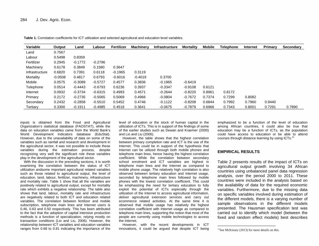
Table 1. Correlation coefficients for ICT utilization and selected agricultural and education level variables.
Variable Output Land Labour Fertilizer Machinery Infrastructure Mortality Mobile Telephone Internet Primary Secondary
Land 0.7567 Labour 0.5498 0.8359 Fertilizer 0.2945 -0.1772 -0.2796 Machinery 0.6178 0.3849 0.1580 0.3647 Infrastructure 0.6820 0.7391 0.6118 -0.1965 0.3119 Mortality -0.0508 0.4817 0.6793 -0.6016 -0.4019 0.3700 Mobile 0.0575 -0.3089 -0.5727 0.4577 0.3836 -0.1965 -0.6419 Telephone 0.0514 -0.4443 -0.6793 0.6236 0.3937 -0.3347 -0.9108 0.6121 Internet 0.0932 -0.3734 -0.6315 0.4993 0.4571 -0.2644 -0.8220 0.8961 0.8172 Primary 0.2172 -0.2735 -0.5065 0.5069 0.4966 -0.0804 -0.7672 0.7374 0.7299 0.8082 Secondary 0.2432 -0.2858 -0.5510 0.5452 0.4746 -0.1122 -0.8208 0.6844 0.7992 0.7960 0.9440 Tertiary 0.3300 -0.1911 -0.4985 0.4518 0.3641 -0.0675 -0.7879 0.6966 0.7343 0.8001 0.7291 0.7890
inputs is obtained from the Food and Agricultural Organization’s statistical database (FAOSTAT), while the data on education variables came from the World Bank’s World Development Indicators database (EduStat). However, due to the unavailability of data on some of the variables such as rainfall and research and development in the agricultural sector, it was not possible to include these variables during the estimation process, despite recognizing very well the significant role these variables play in the development of the agricultural sector.
With the discussion in the preceding sections, it is worth examining the correlation between the status of ICT utilization andsome important agricultural related variables such as those related to agricultural output, the level of education, land, labour, fertilizer, machinery, infrastructure and mortality rate. Table 1 show that all the variables are positively related to agricultural output, except for mortality rate which exhibits a negative relationship. The table also shows that land, labour, mortality rate and infrastructure are negatively related to both ICT and education related variables. The correlation between fertilizer and mobile subscription, telephone main lines and Internet users is 0.46, 0.63 and 0.50 respectively. This has been attributed to the fact that the adoption of capital intensive production methods is a function of specialization, relying mostly on transaction conditions (Lio and Liu, 2006). However, the relationship between ICT variables and education variables ranges from 0.68 to 0.81 indicating the importance of the
level of education or the stock of human capital in the utilization of ICTs. This is in support of the findings of some of the earlier studies such as Dewan and Kraemer (2000) and Lio and Liu (2006).
However, the table shows that the highest correlation between primary completion rate and ICT is the use of the Internet. This could be in support of the hypothesis that Internet can be utilized through both mobile phones and telephone main lines, hence having the highest correlation coefficient. While the correlation between secondary school enrolment and ICT variables are highest in telephone main lines and the Internet as compared to mobile phone usage. The relatively high correlation is also observed between tertiary education and Internet usage, seconded by telephone main lines followed by mobile phones with the lowest correlation coefficient. This could be emphasizing the need for tertiary education to fully exploit the potential of ICTs especially through the utilization of the Internet to access agricultural information, deliver agricultural extension services and carry out ecommerce related activities. At the same time it is observed that mobile usage has relatively the highest correlation coefficient with Internet usage as compared to telephone main lines, supporting the notion that most of the people are currently using mobile technologies to access the Internet.
However, with the recent developments in ICT innovations, it could be argued that despite ICT being
emphasized to be a function of the level of education among African countries, it could also be true that education may be a function of ICTs, as the population could have access to education or be able to attend courses through distance learning by using ICTs.11 EMPIRICAL RESULTS Table 2 presents results of the impact of ICTs on agricultural output growth involving 34 African countries using unbalanced panel data regression analysis, over the period 2000 to 2011. These countries were included in the analysis based on the availability of data for the required economic variables. Furthermore, due to the missing data on specific variables involved during estimation of the different models, there is a varying number of sample observations in the different models presented. The Hausman specification test was carried out to identify which model (between the fixed and random effect models) best describes
11See McKinsey (2013) for more details on this.

the data generation process among the countries involved in the cross-country analyses. From the diagnostic tests in Table 2 it is observed that almost all the models exhibited the presence of either heteroscedasticity or autocorrelation or both, rendering the estimates unreliable and inefficient.
These led to the use of the feasible generalised least squares (FGLS) estimation method, since the approach assumes that, in the case of panel heteroscedasticity, the error variances vary across countries, but remain constant over time and within each country (Lio and Liu, 2006). generally, the results in Model 1 of Table 2 show that all the agricultural input variables had a positive and significant impact on agricultural output (to some extent supporting the results of the correlation coefficients in Table 1, except for livestock, machinery and mortality rate which were either found to be negative or insignificant. Looking at the inclusion of the ICT variables in the model reveals that only telephone main lines have a positive and highly significant impact on agricultural output, while both mobile subscription and Internet usage have insignificant impact on agricultural output showing the underutilization of the two technologies in the agricultural sector. Despite the proliferation of mobile phones, this result could be showing that these technologies, despite being utilised effectively in certain agricultural activities or initiatives12, they have not been able to have a significant impact on agricultural production in the sector at country level on the continent. To some extent supporting the findings of the earlier studies by Lio and Liu (2006) in which an ICT adoption index was used and in Antle (1983) where a country’s transport and communication output was used.
Comparing the size of coefficients between Model 1 with models 1 and 3; it is observed that when the telephone main lines variable is included in the model (that is, Model 3), the size of the coefficients of the variables such as labour, infrastructure, mortality rate, and primary education significantly increase to 0.39, 0.23, -0.726 and 0.14 respectively in Model 3 showing improvement in these variables. While the coefficients for land and livestock variables are reduced from 0.67 and -0.14 in Model 1 to 0.65 and -0.18 in Model 3 respectively. These results, to a greater extent reveal that, even though their has been a significant increase in mobile penetration on the continent over the passed decade, the use of telephone main lines still remains the most highly utilised form of technology hence its relatively higher and significant contribution to the growth of the agricultural sector in comparison to both mobile phones and the Internet. This is mainly due to the telephone main lines contribution to the impact of labour, infrastructure, mortality rate and education. The effect of the ICT variables on the coefficient of labour could be attributed to the fact that in countries with higher ICT penetration,
12 See for example McKinsey (2013) for more details.
Chavula 285 the labour force in the agricultural sector tends to be smaller, while the levels of specialization and division of labour is higher. Hence, leading to the underestimation of the elasticity of labour if the ICT variables are omitted (Lio and Liu, 2006).
In terms of technological developments, increases in agricultural production will depend on the technological capacity to innovate, develop and the diffusion of new technologies and technological techniques which are specifically adapted and utilized based on the existing factor endowments and prices in a particular region or country. Hence the level of education will capture the opportunities and potential that exists in a country for its citizens to acquire the necessary skills as well as their utilization and access to agricultural related knowledge, we tried to capture this by replacing the primary education variable with secondary school and tertiary education variables. Despite the change in the education variables the results from equation 1 across Table 1 and 2 and three show that the education variables have a highly significant impact on agricultural production.
Looking at the impact of education in Model 1 across Tables 2 to 4, the results reveal that, as was the case with the inclusion of ICT variables, all the educational variables are found to exert a positive impact on agricultural output, except for the livestock and machinery variables which are found to be negative and insignificant in some cases. Comparing the size of the coefficients of the conventional agricultural input variables when the educational variables are included in the model, the results show that the size of the coefficient for land decreases as the level of education increases across the results of Model 1 in Tables 2 to 4. With the size of the coefficient being higher in the model with primary education (Table 2, Model 1), and the coefficient for land being reduced from 0.67, to 46 and 0.42 for primary, secondary and tertiary education respectively. This could be due to the fact that after acquiring relatively higher levels of education there tends to be higher levels of migration from rural to urban areas joining non-agricultural sectors, hence leading to reduction in the utilization of agricultural resource endowments leading to reduction in overall agricultural output (Aker and Mbiti, 2010). The same coefficient size reduction is observed for fertilizer as it is reduced from 0.04 in Model 1 in Table 2, to 0.03 in Model 1 in Table 3 for primary and secondary education variables respectively. However the fertilizer coefficient increases to 0.17 when the primary education variable is replaced by the tertiary education variable, which could entail an increase in the utilization of modern technologies and industrial inputs such as the use of higher yielding varieties due to the attainment of tertiary education (Hayami and Ruttan, 1970).13 On the other hand, livestock is found to have an insignificant impact when associated with secondary and tertiary
13 See Hayami and Ruttan (1970) for a related discussion.

286 J. Dev. Agric. Econ.
Table 2. Agricultural production function estimates and ICTs, 2000-2011.
Variable Model 1 Model 2 Model 3 Model 4
Constant 15.92 (0.787)*** 15.91 (0.539)*** 13.9 (0.549)*** 15.2 (0.749)*** Land 0.67 (0.059)*** 0.65 (0.062)*** 0.65 (0.049)*** 0.67 (0.067)*** Labour 0.27 (0.042)*** 0.27 (0.043)*** 0.39 (0.045)*** 0.31 (0.057)*** Fertilizer 0.04 (0.011)*** 0.05 (0.011)*** 0.04 (0.011)*** 0.05 (0.013)*** Livestock -0.14 (0.043)*** -0.12 (0.046)** -0.18 (0.037)*** -0.14 (0.060)** Machinery 0.004 (0.012) -0.004 (0.012) -0.0006 (0.011) 0.001 (0.016) Infrastructure 0.22 (0.041)*** 0.21 (0.042)*** 0.23 (0.038)*** 0.23 (0.051)*** Mortality -1.06 (0.095)*** -1.03 (0.099)*** -0.726 (0.098)*** -1.06 (0.127)*** Primary 0.11 (0.063)* 0.11 (0.073) 0.143 (0.055)*** 0.20 (0.127) Mobile -0.006 (0.018) Telephone lines 0.198 (0.041)*** Internet 0.005 (0.033)
Hausman test (Prob>2 ) 0.3123 0.0009*** 0.0143** 0.1299
Wald test for heteroscedasticity 0.0000*** 0.0000*** Wooldridge test (Prob>F) 0.0046 0.0179** 0.0001*** 0.0067***
Breusch and Pagan test (Prob>2 ) 0.0000*** 0.0000***
No. of observations 138 135 138 138 No. of countries 30 30 30 30
The standard errors are in parenthesis; and *,** and *** denote significance levels below 10, 5 and 1% respectively.
Table 3. Agricultural production function estimates and ICTs, with secondary education, 2000-2011.
Variable Model 1 Model 2 Model 3 Model 4
Constant 14.93 (0.643)*** 15.01 (0.638)*** 13.36 (0.896)*** 14.97(0.674)*** Land 0.46 (0.061)*** 0.47 (0.060)*** 0.50 (0.060)*** 0.48 (0.065)*** Labour 0.40 (0.049)*** 0.42 (0.048)*** 0.42 (0.050)*** 0.38 (0.053)*** Fertilizer 0.03 (0.009)*** 0.03 (0.010)*** 0.03 (0.010)*** 0.03 (0.009)*** Livestock 0.03 (0.047) 0.02 (0.046) 0.05 (0.046) 0.44 (0.049) Machinery 0.01 (0.010) 0.01 (0.011) 0.010 (0.010) 0.010 (0.010) Infrastructure 0.14 (0.042)*** 0.15 (0.041)*** 0.13 (0.041)*** 0.14 (0.044)*** Mortality -0.77 (0.136)*** -0.81 (0.137)*** -0.52 (0.168)*** -0.76 (0.142)*** Secondary 0.01 (0.003)*** 0.01 (0.003)*** 0.010 (0.003)*** 0.01 (0.003)*** Mobile -0.002 (0.001) Telephone lines 0.033 (0.013)** Internet 0.004 (0.005)
Hausman test (Prob>2 ) Prob>
2 11.97 (0.3123) 14.15 (0.1172) 12.19 (0.2029) 11.14 (0.26060) Wald test for heteroscedasticity Wooldridge test (Prob>F) 8.656 (0.0073***) 8.613 (0.0074***) 33.057 (0.0000***) 8.867(0.0067***)
Breusch and Pagan test (Prob>2 ) 210.95 (0.0000***) 208.40 (0.0000***) 207.78 (0.0000***) 205.74 (0.0000***)
No. of observations 130 129 130 130 No. of countries 26 26 26 26
The standard errors are in parenthesis; and *,** and *** denote significance levels below 10, 5 and 1% respectively. education, while it is found to be negative and highly significant at conventional levels when associated with primary education. This could be due the fact that in most rural areas where peoples’ livelihood depends entirely on agriculture, students are encouraged to take care of their
livestock at the expense of schooling hence the negative impact. The same result is observed as machinery is found to have a negative and significant effect only when associated with tertiary education variable. This to some extent could be showing that the human capital

Chavula 287 Table 4. Agricultural production function estimates and ICTs, with tertiary education, 2000-2011.
Variable Model 1 Model 2 Model 3 Model 4
Constant 13.34 (0.320)*** 13.34 (0.336)*** 9.98 (0.649)*** 12.5 (0.413)*** Land 0.42 (0.033)*** 0.42 (0.06)*** 0.69 (0.060)*** 0.44 (0.038)*** Labour 0.29 (0.021)*** 0.29 (0.024)*** 0.20 (0.034)*** 0.26 (0.025)*** Fertilizer 0.17 (0.012)*** 0.17 (0.013)*** 0.04 (0.011)*** 0.16 (0.013)*** Livestock 0.01 (0.023) 0.01 (0.027) 0.51 (0.030)* 0.04 (0.025) Machinery -0.004 (0.015)** -0.04 (0.016)** -0.0006 (0.009) -0.05 (0.015)*** Infrastructure 0.37 (0.022)*** 0.37 (0.022)*** 0.29 (0.031)*** 0.37 (0.025)*** Mortality -0.57 (0.076)*** -0.58 (0.078)*** -0.32 (0.107) -0.42 (0.086)*** Tertiary 0.03 (0.005)*** 0.03 (0.005) 0.023 (0.006)*** 0.03 (0.005)*** Mobile 0.001 (0.001) Telephone lines 0.09 (0.011)*** Internet 0.03 (0.004)***
Hausman test (2 ) (Prob>
2 ) 76.85 (0.0000***) 34.14 (0.0001***) 47.61 (0.000****) 48.15 (0.0000***)
Wald test for hetero. (2 ) (Prob>
2 ) 1892.28 (0.0000***) 7.8e+28 (0.0000***) 9.0e+23 (0.0000***) 3.0e+28 (0.0000***) Wooldridge test (F(1,18)) (Prob>F) 2.557 (0.1272) 2.605 (0.1239) 9.527 (0.0064***) 2.520 (0.1298)
Breusch and Pagan test (Prob>2 ) 0.0000***
No. of observations 116 115 113 116 No. of countries 28 28 25 28
The standard errors are in parenthesis; and *,** and *** denote significance levels below 10, 5 and 1% respectively. development might not be fully supporting the technological acquisition, assimilation and utilization since machinery and fertilizer are capturing the effects of the whole range of inputs supplied by the industrial sector which carry modern mechanical and biological technologies (Hayani and Ruttan, 1970).
It has been argued theoretically and empirically that human capital has direct influence on agricultural productivity by affecting the way in which inputs are used and combined by farmers (Mundlak et al., 2008). It also affects one’s ability to adapt and utilize technology to a particular situation or changing needs of individuals or communities. It has also been argued that improvements in human capital affect the acquisition, assimilation and utilization of ICTs (Juma, 2006). To substantiate the correlation between ICTs and human capital variables, which is exhibited to be very high in Table 1, we try to assess to what extent this relationship impacts agricultural production. In general, as was the case with the findings by Lio and Liu (2006), when educational variables are included as a measure of human capital in the agricultural production function together with ICT variables, the results reveal a considerable variation in the size of the coefficients of ICT variables. Among the three ICT variables, the results reveal that telephone main lines exert, relatively, the highest impact on agricultural productivity irrespective of the level of education. This could be mostly be due to the wide spread of telephone main lines as they remain accessible to the rural masses whose livelihoods mostly depend on
the agricultural sector and does not really require some exceptional educational skills to be utilised. However, the size of its coefficient is largest when associated with primary education, than when associated with secondary and tertiary education (with the second largest) levels. And also the Internet has a statistically significant impact on agricultural production at conventional levels only when it is associated with tertiary education.
However, when mobile phones are included as an ICT variable, the results show that mobile penetration does not have any significant impact on agricultural output when associated with any of the educational levels. This in some cases should mean that people (no matter their level of education) do not effectively put mobile phones to their productive use in the agricultural sector in Africa, especially by exploiting their technological potential to the benefit of the sector, taking into consideration also the challenges in having access to electricity in the rural areas where a greater percentage of the population involved in agricultural activities is based. To a greater extent this could mean that despite the wide spread of mobile phones on the continent, mobile technologies have not been effectively utilized in the agricultural sector to enhance agricultural production. The different countries have not fully utilized the potential that comes with the utilization of the Internet for agricultural growth, as the continent, relatively, still makes more use of telephone main lines. Also, scaling up for most of existing technology based services is a difficult issue and also the penetration of smart phones and tablets among African

288 J. Dev. Agric. Econ. farmers remains low, limiting the full exploitation of the potential that comes with ICT-based agricultural technologies. Since a greater part of the population engaged in agricultural activities is in the rural areas, where access to energy sources like electricity is very low, it implies a low usage of some ICT-based technologies e.g. mobile technologies, hence the failure to put them technologies into effective use.
The results also show that the impact of infrastructure is highest when associated with tertiary education, but decreases when telephone main lines are included in the model, while the impact of infrastructure increases significantly with ICTs especially when associated with primary education. With reference to mortality rate, the results show that there is a decreasing impact on mortality rate as the level of education increases, and much more decreases are experienced when mortality rate is associated with the utilisation of ICTs. Conclusion The study is triggered by the desire to assess if at all the proliferation of ICTs, especially due to the growth of mobile technologies on the African continent have had any significant impact on agricultural production. This was further motivated by the view that there exists a gap in empirical research with regard to the assessment of the impact of ICTs on agricultural production on the continent. The study uses the 2000 to 2011 panel data for 34 African countries to examine the impact of ICTs on agricultural production, since it was since the late 1990s when the spread of ICTs especially mobile and Internet technologies started having an impact on the continent. It extends the study by Antle (1983) on the impact of the transport and communication infrastructure on agricultural productivity, by applying the methodology and approach to the African continent and by utilizing specific ICT variables which include the number of mobile subscribers, Internet users and telephone main lines among African countries. The study is envisaged to play a greater role in filing the gap that exists on the African continent, especially during this period when Africa has become the fastest growing region in the global telecommunications market.
The empirical analysis results suggest that ICTs play a significant role in enhancing agricultural production, and the use of telephone main lines remains a significant contributor to agricultural growth despite the wide proliferation of mobile phones. The evidence also suggests that despite both mobile phones and telephone main lines being utilized to access the Internet, its impact falls behind that of telephone main lines, to some extent suggesting that there is low usage of ICTs, especially the Internet for carrying out activities with significant contribution to agricultural growth on the continent. Internet usage has not yet reached a “critical mass” that could fully exploit network externalities, hence contribute
significantly to agricultural production in Africa. Therefore, there is need for African governments to continue promoting the use of the Internet in carrying out agricultural activities, so as to reach a “critical mass” of users needed to enable the sector exploit unique opportunities that come with the use of the Internet and hence contribute significantly to agricultural growth.
The empirical evidence from this study also suggests that certain socio-economic characteristics such as higher education levels and skills are prerequisites for effective improvements in agricultural production. This is observed in the analysis when education level variables are included in the agricultural production function as input variables, which in general, considerably reduce the estimated production elasticity of the ICT variables, suggesting to some extent the minimal emphasis with regard to the utilization of ICTs in the sector. However, the results show that despite the level of education, telephone main lines seem to have a relatively higher impact on agricultural output as compared to mobile and Internet usage. The results also show that despite the level of education, mobile penetration does not seem to have any significant impact on agricultural production. This result to a greater extent signifies the lack of innovative capacity or underutilization of mobile technologies in enhancing agricultural production on the continent.
This calls for African governments to invest in technological capacity, especially in higher education, to innovate, develop and disseminate new technologies and technological techniques in order to increase agricultural production. Especially, since it has been observed that given the available technology used by farmers over generations in Africa, agricultural extension does not play a significant role in agricultural productivity unless new profitable technologies are developed (Otsuka, 2006). Human capacity development especially through education is the key element of a knowledge-based, innovation driven economy as it affects both the supply and demand for technological innovation and utilization. Human capital and skilled labour complement technological advances, and new technologies cannot be adopted without a sufficiently educated and trained workforce. Governments should also put emphasis on public policies that support investments in ICT infrastructure.
Furthermore focus on the development and spread, especially through development of broadband technologies, in order to ensure affordable and reliable ICT access to almost all corners of each and every country, as most of the farmers are based in rural areas. This will not only provide new opportunities for rural farmers to have access to information on agricultural technologies, but also to use ICTs in agricultural services such as the countries’ agricultural extension services. There is need for governments to increase their commitment to productive investments such as agricultural research, technology and rural infrastructure,
rather than putting more emphasis and committing a lot of resources to direct farm subsidy initiatives. Conflict of Interests The author(s) have not declared any conflict of interests. REFERENCES AfDB, OECD, UNDP, UNECA (2012). African Economic Outlook 2012:
Promoting Youth Employment. www.africaneconomicoutlook.org/en Aker JC, Mbiti IM (2010). Mobile phones and economic development in
Africa. J. Econ. Perspect. 24(3):207-232. http://dx.doi.org/10.1257/jep.24.3.207
Aker JC (2011). Dial “A” for Agriculture: A Review of Information and Communication Technologies for Agricultural Extension in Developing Countries. Paper presented at the Agriculture for Development Conference, University of California – Berkely.
Ansoms A (2008). Striving for growth, bypassing the poor? A critical review of Rwanda’s rural sector policies. Journal Modern Afr. Stud.
46:1-32. http://dx.doi.org/10.1017/S0022278X07003059 Antle JS (1983). Infrastructure and aggregare Agriculture Productivity:
International Evidence. Econ. Develop. Cult. Change. 31(3):609-619. http://dx.doi.org/10.1086/451344
Burgess R, Pande R (2005). Do Rural Banks Matter? Evidence from the Indian Social Banking Experiment. Am. Econ. Rev. 95(3):780-95. http://dx.doi.org/10.1257/0002828054201242
Chavula HK (2012). Telecommunications Development and Economic Growth in Africa. J. Infor. Technol. Develop. 19(1):5-23. http://dx.doi.org/10.1080/02681102.2012.694794
Chavula HK, Chekol A (2010). ICT Policy Development Process in Africa. Int. J. ICT Res. Develop. Afr. 2(3):20-45.
Dahlan C (2007). The Challenge of the Knowledge Economy for Latin America, Globalisation, Competit. Governabil. J. 1:1.
Dewan S, Kreamer KL (2000). Information Technology and Productivity: Evidence from Country-Level Data. Manage. Sci. 46(4):548-562. http://dx.doi.org/10.1287/mnsc.46.4.548.12057
Driouchi A, Azelmad E, Anders GC (2006). An Econometric Analysis of the Role of Knowledge in Economic Performance. J. Technol. Trans. 31:241-255. http://dx.doi.org/10.1007/s10961-005-6109-9
EIU (2012). Into Africa: Emerging Opportunities for Business. www.eiu.com. Accessed December 2012.
GSMA (2011). Driving economic and social development through mobile services. African Mobile Observatory 2011, GSMA. Retrieved fromhttp://www.gsma.com/publicpolicy/wp-content/uploads/2012/04/africamoeswebfinal.pdf
Halewood NJ, Surya P (2012). Mobilising the Agricultural Value Chain. In 2012 Information and Communication for Development – Maximising Mobile, World Bank, Washington D.C.
Hayami Y, Ruttan VW (1970). Agricultural Productivity Differences among Countries. Am. Econ. Rev. 60(5):895-911.
ITU (2011). World Telelcommunication Indicators Database, Geneva. 2011.
Juma C (2006). Reinventing growth:Science, technology and innovation in Africa. Int. J. Technol Global. 2(¾):323-339.
Kimenyi MS, Moyo N (2011). Leapfrogging Development Through Technology Adoption. In Foresight Africa: The Continent’s Greatest Challenges and Opportunities for 2011, Africa Growth Innitiative, The Brookings Institution.
Chavula 289 Levine R (2005a). Finance and Growth: Theory and Evidence. In
Handbook of Economic Growth, ed. Philippe Aghion and Seven Durlauf. The Netherlands: Elsev. Sci.
Levine R (2005b). Finance and Growth: Theory and Evidence. NBER Working Paper 10766. www.nber.org/papers/w10766. Accessed December 2012.
Lio M, Liu M (2006). ICT and Agricultural Productivity: Evidence from cross-country data. Agric. Econ. 34:221-228. http://dx.doi.org/10.1111/j.1574-0864.2006.00120.x
McKinsey (2011). Sizing Africa’s Agricultural Opportunity. In Four lessons for transforming African Agriculture, McKinsey Quarterly, April, 2011. McKinsey & Company.McKinsey (2013). Lions go digital: The Internet’s transformative potential in Africa, on www.mckinsey.com. Accessed in December 2013.
Mundlak Y, Butzer R, Larson D (2008). Heterogenous Technology and Panel Data: The Case of the Agricultural Production. Policy Research Working Paper (WPS 4536), Development Research Group, The World Bank, Washington DC.
Mundlak Y, Larson D, Butzer R (1997). The Determinants of Agricultural Production: A Cross-Country Analysis. Policy Research Working Paper (WPS 1827), Development Research Group. The World Bank, Washington DC. http://dx.doi.org/10.1596/1813-9450-1827
Muto M, Yamano T (2009). The Impact of Mobile Phone Coverage Expansion on Market Participation: Panel Data Evidence from Uganda. World Develop. 37(12):1887-96. http://dx.doi.org/10.1016/j.worlddev.2009.05.004
OECD, AfDB, UNECA (2009). The African Economic Outlook (AEO) 2009 on Innovation and New Technologies in Africa, OECD Printing Press.
Otsuka K (2006). Why can’t we transform traditional agriculture in Sub-Saharan Africa? Rev. Agric. Econ. 28(3):332-337. http://dx.doi.org/10.1111/j.1467-9353.2006.00295.x
Rao M (2011). Mobile Africa Report 2011: Regional Hubs of Excellence and Innovation, accessed at www.mobilemonday.net/reports/MobileAfrica_2011.pdf
Roeller L, Waverman L (2001). Telecommunications Infrastructure an Economic Development: A Simulataneous Approach. Am. Econ. Rev. 91(4):909-923. http://dx.doi.org/10.1257/aer.91.4.909 Sen S, Choudhary V (2011). ICT Applications for Agricultural Risk Management. ICT in Agriculture Sourcebook. Washington D.C. World Bank.
UNECA (2007). Economic Report on Africa 2007: Accelerating Africa’s development through diversification. UNECA, Addis Ababa, Ethiopia.
UNECA (2012). Economic Report on Africa 2012: Unleashing Africa’s potential as a pole for global growth, UNECA, Addis Ababa, Ethiopia.
World Bank, AfDB, AUC (2012). The Transformational use of Information and Communication Technologies in Africa on http://siteresources.worldbank.org/EXTINFORMATIONANDCOMMUNICATIONANDTECHNOLOGIES/Resources/282822-1346223280837/MainReport.pdf. Accessed December 2012.

Vol. 6(7), pp. 290-298, July, 2014 DOI: 10.5897/JDAE2014.0567 Article Number: BEF7A9045620 ISSN 2006-9774 Copyright © 2014 Author(s) retain the copyright of this article http://www.academicjournals.org/JDAE
Journal of Development and Agricultural Economics
Full Length Research Paper
An economic analysis of crude oil pollution effects on crop farms in Rivers State, Nigeria
ThankGod Peter Ojimba1*, Jacob Akintola2, Sixtus O. Anyanwu1 and Hubbert A. Manilla1
1Department of Agricultural Science, Ignatius Ajuru University of Education,Ndele Campus, P.M.B. 5047,
Port Harcourt, Nigeria. 2Department of Agricultural Economics, Bowen University,Iwo, Osun State, Nigeria.
Received 6 March, 2014; Accepted 9 May, 2014
This study researched on crude oil pollution effects on crop farms in Rivers State, Nigeria using stochastic translog production function. Data were collected in the state, using multi-stage sampling technique. A total of 296 structured questionnaires retrieved from farmers in crude oil polluted and non-polluted areas of the state were used. Stochastic translog production interaction between land and heavy, medium and light oil spillages resulted in crops output reduction by 0.255, 1.257 and 1.027 units, respectively. Interaction across heavy, medium and light oil spillages and fertilizers usage indicated farm crops output decrease by 0.805, 0.586 and 0.729 units, respectively. This study therefore concluded that crude oil pollution on crops farms reduced crops output significantly, hence detrimental to crop production in Rivers State, Nigeria. Key words: Crude oil, pollution, stochastic translog production function, crops output, Nigeria.
INTRODUCTION The petroleum industry is the backbone of the Nigeria economy, accounting for over 90% of total foreign exchange revenue. The daily production of crude oil is slightly above two million barrels from more than 240 producing fields, totaling over 5,284 wells drilled. With over half a century of oil and gas exploration, exploitation and production, Nigeria has built up a considerable hydrocarbon infrastructure with over 7,000 km of pipelines linking over 280 producing flow stations all of which are situated in the Niger Delta region of Nigeria (Niger Delta Development Commission, 2006). The Niger Delta region is situated in the southern part of Nigeria and bordered to the south by the Atlantic Ocean, occupying a surface area of about 112, 110 km2, which represents 12% of Nigeria total surface area with an
estimated population of about 28 million inhabitants in 2006 (NDDC, 2006). Within this region, crude oil pollution such as oil spillages and gas flaring regularly occur (Orji, et al., 2011; Nwaichi and Uzazobona, 2011).
Scholars such as Uzoho et al. (2004) evaluated the influence of crude oil on maize growth and soil properties in Ihiagwa, Imo State, Nigeria. The results of their study showed that seed germination, plant height, leaf area and dry matter yield significantly deceased as the levels of crude oil pollution increased. The primary way in which crude oil pollution reduced crop growth and performance according to their study was through reduction of seedling emergence and direct suffocation of plant and oxygen diffusion rates between soil system and the atmosphere.
*Corresponding author.E-mail: [email protected] Author(s) agree that this article remain permanently open access under the terms of the Creative Commons Attribution License 4.0 International License

Dung et al. (2008) explored the spatial variability effects of gas flaring on the growth and development of cassava (Manihot esculenta), water leaf (Talinum triangulare) and pepper (Piper spp.), which are crops commonly cultivated in the Niger Delta. Their results suggested that a spatial gradient exist in the effect of gas on crop development. Retardation in crop development manifested in decreased dimensions of leaf lengths, and widths of cassava and pepper crops closer to the gas flare points. Their statistical analysis confirmed that cassava yield were higher at locations further away from the flare point. In addition, the amount of starch and ascorbic acid in cassava decreased when plant is grown closer to the gas flare. High temperature around the gas flare appeared to be the most likely cause of the retardation and low yield.
Okonwu et al. (2010) investigation showed that the percentage of germination of maize (Zea mays) decreased with increase in concentration of crude oil equilibrated with water. Germination rate decreased significantly with increased time of pre-soaking in crude oils. Crude oil spilled soil immediately after planting increased the length of lag phase preceding germination from 100% in the control to 58% in crude oil contaminated soil. Fernandez-Luqueno et al. (2012) studied the ability of various crops to grow and maintain their yield when they are cultivated in contaminated soils, thereby being able to choose the most appropriate crop when suddenly a gasoline-pipeline collapse on soil of subsistence agricultural systems. Their results showed that gasoline contamination reduced seedling emergence, shoot length, root volume, root dry weight, shoot dry weight and abundance of nodules. Problem statement Despite the availability and use of advanced technology in the petroleum industry, various forms of accidents such as blow-outs of production wells, explosions and pipeline ruptures still occur, which are worsened by vandalization of oil installations and pipelines (Otitoloju et al. 2007; Iturbe et al. 2008; Li et al., 2011). Farmers in Rivers State are eventually the most affected judging by the death of marine and terrestrial organisms usually involved in oil spill incidents and the hazardous effect of gas flaring (Saier, 2006; Otitoloju and Dan-Patrick, 2010; Huang, et al., 2011). The rivers and underground water which the inhabitants rely on, for their drinking water have been polluted with crude oil, while buildings and agricultural products had been destroyed (Atakpo and Ayolabi, 2009; Ekpoh and Obia, 2010; Nwaichi and Uzazobona, 2011; Onyenekenwa, 2011). Irregularities had been observed in the major livelihood activities of the people of Rivers State of Nigeria due to crude oil pollution (Okoli, 2006; Adoki and Orugbani, 2007; Orogun, 2009).
Ekunwe and Orewa (2007) (examined the technical efficiency and productivity of yam in Kogi State of Nigeria using stochastic frontier production function.
Ojimba et al. 291 The result indicated that the technical efficiency of farmers varied with a mean of 62%, while only about 23% of the farmers had technical efficiencies exceeding 80%. Erhabor and Emokaro (2007) employed the use of the stochastic frontier production function in the comparative economic analysis of the relative technical efficiency of cassava farmers in the three agro-ecological zones of Edo State, Nigeria. The empirical estimates showed mean technical efficiency of 72, 83 and 91% for Edo South, Edo North and Edo Central agro-ecological zones, respectively. Ajani and Ugwu (2008) used a stochastic production frontier model and obtained the result that gamma which is a measure of variance of output from the frontier attributed to efficiency was 0.114.
Heady et al. (2010) presented multi-output, multi-input total factor productivity (TFP) growth rate in agriculture for 88 countries over the 1970 and 2001 period estimated with both stochastic frontier analysis (SFA) and data envelopment analysis (DEA). They found results with SFA to be more plausible than with DEA, and used them to analyze trends across countries. Large volumes of literature still exist that had used stochastic frontier production analysis in crop production (Ali, 1996; Onyenweaku and Okoye, 2007; Nyagaka et al., 2010; Dlamini et al; 2010). Some scholars (Lachaal et al., 2005; Awoyemi and Adeoti, 2006; Managi et al., 2007) have studied some aspects of stochastic frontier production function but they did not study the economic analysis of crude oil pollution effects on crop farms in Rivers State.
Therefore, there is a dearth of literature on the use of stochastic frontier transcendental logarithmic (traslog) production function for an economic analysis of crude oil polluted and non-polluted crop farms in Rivers State, Nigeria. At this juncture one may seek to understand the economic analysis of crude oil pollution effects on crop farms in Rivers State, Nigeria, using the stochastic frontier transcendental logarithmic (translog) production function as analytical tool to bridge this gap in knowledge. The objectives of the study
The main objective of this study is to estimate economically crude oil pollution effects on crop farms in Rivers State, Nigeria using stochastic translog production function approach. The specific objectives are to:
1. Determine crude oil pollution effects on crop farms in Rivers State, Nigeria using stochastic translog production function analysis. 2. Make policy statements that could ameliorate the effects of crude oil pollution on crop farms in Rivers State, Nigeria. MATERIALS AND METHODS Data collection This study was conducted in Rivers State of Nigeria in 2003. Data

292 J. Dev. Agric. Econ. were collected from both the primary and secondary sources. The primary data were collected through personal interviews and observation with the farmers, and structured questionnaires were distributed among farmers in crude oil polluted and non-crude oil polluted areas of an affected community in the state. A multistage sampling technique was used to obtain data for the study. The first stage involved the selection of 17 local government areas (LGAs) out of the existing 23 LGAs in Rivers State. The selected LGAs include: Abua/Odual, Ahoada East, Ahoada West, Andoni, Asaritoru, Degema, Eleme, Emohua, Etche, Gokana, Ikwerre, Khana, Obio/Akpor, Ogba/Egbema/Ndoni, Omuma, Oyigbo and Tai LGAs. These 17 LGAs were selected based on the fact that they were more crop farming inclined than others. The second stage involved the stratification of farmland in a selected LGA into two sampling units namely crude oil polluted and non-crude oil polluted. This stratification of the farmland into two sampling units was based on the fact that information were needed from both crude oil polluted and non-polluted areas.
The third stage involved the random sampling of 10 farmers from crude oil polluted areas in a selected LGA and a corresponding number of 10 farmers from non-crude oil polluted farms (non-polluted) in the same locality (community) in the given area. This gave a total of 20 farmers interviewed per selected LGA in the State, giving a total of 340 questionnaires distributed in the 17 LGAs selected. Out of 340 questionnaires administered, due to difficult terrain, the politicking of oil pollution issues and youth restiveness in the State as at the time of the survey, only 326 questionnaires were retrieved. Furthermore, 30 questionnaires were found inconsistent with the set objectives of the study. Hence, only a total of 296 questionnaires were retained as suitable for analysis. Out of these 296 questionnaires retained as suitable for analysis, 169 questionnaires were retrieved from the crude oil polluted farms and 127 questionnaires from non-polluted farms. The unequal weighting in the data analyzed arose because most of the discarded and unretrieved questionnaires belonged to the non-polluted farms category. Because of the large number of samples retrieved from both polluted and non-polluted crop farms, comparison between the two groups of farms as a measure of efficiency was adequate and not misleading. Measurement of crude oil pollution and technology indices To measure the negative effects of crude oil pollution on each farmland polluted, the impact of crude oil pollution index was estimated following the methods specified by Mubana (1978), and Canter and Hill (1979) modified as follows:
(1) where, P= crude oil pollution index per farmer in the crude oil polluted areas; q2i = land affected by the crude oil pollution, indicating the farm’s degree of crude oil pollution (ha). q1 = total land area cultivated (ha) Xi = percentage of crop yield foregone due to oil pollution (where, i = farmers degrees of pollution, 93 to 100%, 31 to 92% and 0 to 30%). n = types of crude oil pollution affecting individual farm: n1 = heavy oil pollution (acquired land); n2 = medium oil pollution ; n3 = light oil pollution Xi was adopted from Udo and Fayemi (1975) and Mubana (1978), which categorized the types of negative effects of oil pollution: Category A (ni): (i) Heavy oil spillage which leads to 93 to 100% crop yield loss.
(ii) Acquired land for oil well – head sites, flow stations, drilling sites, oil field location, borrow pits, gas flaring sites, pipeline laying operations and other oil related activities which leads to 100% crop yield loss (Mubana, 1978); Category B (n2): Medium oil spillage which leads to 31 to 92% crop yield reduction; Category C (n3): Light oil spillage which leads to 0 to 30% crop yield reduction. The level of technology was captured using in a chain index method proposed the Harper (1971) and Mubana (1978). It is mathematically expressed as:
(2) Where, T = level of technology index, 2i = quantity of each technology type used in current year t, (2003) measured in bags of fertilizers, packets of improved seeds and dressing of seeds. These inputs were converted into percentages before the summations; 1i = quantity of each technology type used in year t - 1, (2002) measured as above, i = 1,2, …. 296, K = number of types of technology adopted by the farmer in t (2003) and t-1 (year (2002) 2.3 Stochastic translog production function Christensen et al. (1973) studied translog production function which is general, flexible and allowed analysis of interactions among variables. Ali (1996) used stochastic translog production function to analyse socio-economic determinants of sustainable crop production in Nepal. This study will apply the stochastic translog production function with moderation from Christensen et al. (1973) and Ali (1996) to estimate economically crude oil pollution effects on crop farms in Rivers State, Nigeria. The stochastic frontier translog production function given in equation (3) was estimated for the crude oil polluted crop farms only, while the estimation of non-polluted crop farms did not include the P variables. The general form of the translog stochastic production function used in this study is:
ln Yj = 0 + ailnXij + ½ big (lnXijlnXij)
+ ckln Pkj + dt lnTtj + bii ( lnXii)2
+ ½ eik (lnXijlnPkj) + ½ fit (lnXij lnTtj)
+ ½ hkk (ln Pkj ln Pkj) + ½ rkt (ln Pkt lnTtj)
+ ½ stt (lnTtjlnTtj) + uj +vi
i=1 i=1 g=1
i=1 k=1
n m
i=j t=1
n p
k=1 k=1
m m
k=j t=1
n p
t=1 t=1
p
n n n
i=1
m
t=1
n
i=1
p
p
(3) where, j = 1,2,3, ……… 169 for crude oil polluted crop farms and

127 for non-polluted crop farms i = 1,2,3, are physical inputs.
Parameters used include: Y = Crop output in ton/ha per farmer (crops here refer to different types of crops because of the subsistence nature of production – mixed cropping). X = Vector of physical inputs used (land area cultivated in hectares, available family and hired labor in man days; fixed and operating capital in dollars). P = Vector of effect of crude oil pollution index on the farmer; T=Vector of level of technology index; vi=Random error due to misspecification of the model; ui =Ratio of actual value to maximum possible output, that is inefficiency component of error terms. ln = logarithmic sign = parameter of intercept, ai = parameters of physical inputs, bijg = parameters for interaction across ith and gth physical inputs, ck = parameters of crude oil pollution variables in indices, dr = parameters for level of technology variables indices, bii = parameters for squared terms of physical inputs. eik = parameters for interaction between physical inputs and crude oil pollution variables fit = parameters for interaction between physical inputs and technology variables. hkk= parameters for interaction among crude oil pollution variables, rkt = parameters for interaction between oil pollution and technology variables, stt= parameters for interaction across technology variables It is important to note that Xi and T variables are some conventional physical inputs and technology variables normally considered in transformation process. However, the P variables are the conditioning variables which had been included into the model to capture the negative and detrimental effects of crude oil pollution on crops output or yield.
Translog model specifications
The model specifications for the translog stochastic production function retained in Equation (3) for the crude oil polluted crop farms is as given in Equation (4). As earlier mentioned, the specification for the non-polluted crop farms category excluded the crude oil pollution variables, that is X5 to X12, and their various interactions. ln Y = 0 + 1 ln X1 + 2 ln X2 + 3 ln X3 + 4 ln X4 + 5 ln X5
+ 6 ln X6 + 7 ln X7 + 8 ln X8 + 9 ln X9 + 10 ln X10
+ 11 ln X11 + 12 ln X12 + 13 ln X13+ 14 ln X14 + 15 (lnX1)2
+ 16 (lnX2)2
+ 17 (lnX3)2
+ 18 (lnX1 . ln X2)
+19 (lnX1 . ln X3) + 20 (lnX2 .
ln X3) + 21 (lnX1 . ln X10)
+22 (lnX1 . ln X11) + +23 (lnX1
. ln X12) +24 (lnX1 . ln X13)
+25 (lnX1 . ln X14) +26 (lnX2
. ln X13) +27 (lnX10 . ln X11)
+28 (lnX10 . ln X12) +29 (lnX11
. . ln X12) +30(lnX10 . ln X13)
+31 (lnX11 . ln X13) +32 (lnX12
. ln X13) +33 (lnX4 . ln X13)
+34 (lnX4 . ln X14) +35 (lnX13
. ln X14) + u + v (4)
Ojimba et al. 293 It is necessary to explain here that the total number of possible interactions were 75 but these had been drastically reduced to 21 interactions only. In addition to the 14 sets of variables considered in this analysis, the number of parameters estimated increased to 36 (including the intercept). This was done in order to ensure that only economically meaningful and theoretically plausible interactions were retained for the analysis, and also to reduce and ease the computation burden, as well as reduce the risks of multicollinearity.
RESULTS AND DISCUSSION Table 1 shows the results of maximum likelihood estimation (MLE) for stochastic translog production frontier function in crude oil polluted and non-polluted crop farms in Rivers State, Nigeria. The results will be analyzed following the various types of variables and interactions obtained according to the translog model specification as shown in equation (4). Stochastic translog production variables interactions The discussions concentrated on the interactive actions of the translog variables used in the analysis Squared terms of physical inputs (bii) Doubling the physical inputs means, using these inputs once again after the initial usage on crude oil spilled farms with the intension of increasing productivity after the application of proper remediation techniques in crude oil polluted crop farms, while in the non–polluted crop farms, it means doubling the usage of these inputs with the sole purpose of increasing production. Therefore, squaring (doubling) the amount of farm land (15) available for farming in crude oil polluted farms decreased the crop output by 0.093 units, though marginal.
There was an increase of 0.051 units per unit of output experienced in non-polluted crop farms when farmland was doubled (squared), though also marginal inelastic and not significant. These results showed that when amount of farmland available was doubled, there was an increase in output in non-polluted crop farms, and a decrease in farm output in crude oil polluted crop farms category. This could be due to the environmental stress or negative effects of crude oil pollution on crops (Achuba, 2006).
Squaring the labour variable ( 16) (labour x labour) in crude oil polluted crop farms reduced output by 0.112 units, and at the same time led to increased cost of production, whereas, if labour was doubled in non-polluted crop farms, crop output increased, though marginally by 0.150 units (significant at 1% level) despite the increased cost of production. Squaring of capital
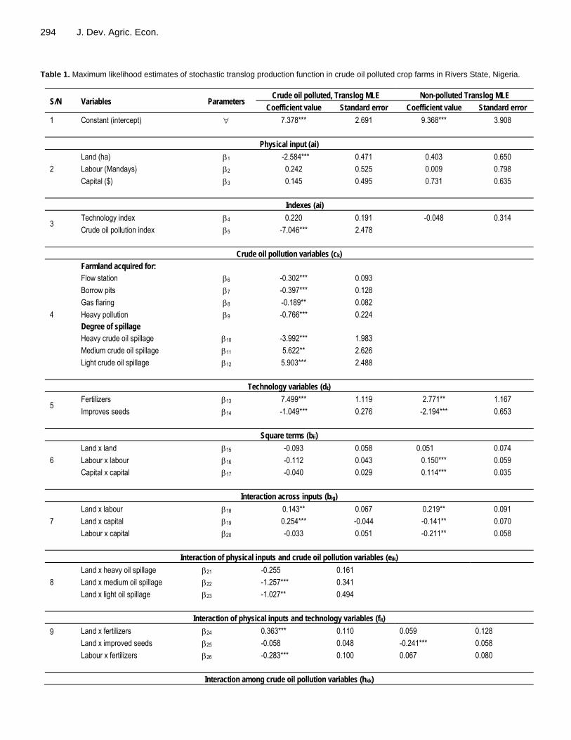
294 J. Dev. Agric. Econ. Table 1. Maximum likelihood estimates of stochastic translog production function in crude oil polluted crop farms in Rivers State, Nigeria.
S/N Variables Parameters Crude oil polluted, Translog MLE Non-polluted Translog MLE
Coefficient value Standard error Coefficient value Standard error
1 Constant (intercept) 7.378*** 2.691 9.368*** 3.908
Physical input (ai)
2
Land (ha) 1 -2.584*** 0.471 0.403 0.650
Labour (Mandays) 2 0.242 0.525 0.009 0.798
Capital ($) 3 0.145 0.495 0.731 0.635
Indexes (ai)
3 Technology index 4 0.220 0.191 -0.048 0.314
Crude oil pollution index 5 -7.046*** 2.478
Crude oil pollution variables (ck)
4
Farmland acquired for:
Flow station 6 -0.302*** 0.093
Borrow pits 7 -0.397*** 0.128
Gas flaring 8 -0.189** 0.082
Heavy pollution 9 -0.766*** 0.224 Degree of spillage Heavy crude oil spillage 10 -3.992*** 1.983
Medium crude oil spillage 11 5.622** 2.626
Light crude oil spillage 12 5.903*** 2.488
Technology variables (dt)
5 Fertilizers 13 7.499*** 1.119 2.771** 1.167
Improves seeds 14 -1.049*** 0.276 -2.194*** 0.653
Square terms (bii)
6
Land x land 15 -0.093 0.058 0.051 0.074
Labour x labour 16 -0.112 0.043 0.150*** 0.059
Capital x capital 17 -0.040 0.029 0.114*** 0.035
Interaction across inputs (big)
7
Land x labour 18 0.143** 0.067 0.219** 0.091
Land x capital 19 0.254*** -0.044 -0.141** 0.070
Labour x capital 20 -0.033 0.051 -0.211** 0.058
Interaction of physical inputs and crude oil pollution variables (eik)
8
Land x heavy oil spillage 21 -0.255 0.161
Land x medium oil spillage 22 -1.257*** 0.341
Land x light oil spillage 23 -1.027** 0.494
Interaction of physical inputs and technology variables (fit)
9
Land x fertilizers 24 0.363*** 0.110 0.059 0.128
Land x improved seeds 25 -0.058 0.048 -0.241*** 0.058
Labour x fertilizers 26 -0.283*** 0.100 0.067 0.080
Interaction among crude oil pollution variables (hkk)

Ojimba et al. 295 Table 1. Contd.
10
Heavy spillage x medium spillage 27 -1.244* 0.709
Heavy spillage x light spillage 28 -1.042* 0.647
Medium spillage x light spillage 29 -0.326** 0.153
Interaction between crude oil pollution and technology variables (rkt)
11
Heavy spillage x fertilizers 30 -0.805*** 0.224
Medium spillage x fertilizers 31 -0.586*** 0.210
Light spillage x fertilizers 32 -0.792* 0.389
Interaction across technology variables (Stt)
12
Technology index x fertilizers 33 -0.312*** 0.094 -0.547*** 0.109
Technology index improved seeds 34 0.656*** 0.202 0.060 0.042
Fertilizers x improved seeds 35 -0.102* 0.062 0.045 0.062
0.863 - 0.9999 -
3.109*** 0.950 190.634 698.59 σ 0.621*** 0.030 0.883*** 0.028 δu2 0.350 - 0.780 - δv2 0.03620 - 0.00002 - Log likelihood function -658.252 - -733.206 - Average technical efficiency 0.586 - 0.664 - F-test 26.37*** - 16.21*** -
Source: Field survey, 2003. Asterisks indicate significant level: ***1%; **5%; *10%. (17) decreased output in crude oil polluted crop farms by 0.040 units, with a possible increase in cost of production.
However, in non-polluted crop farms output increased when capital was squared by 0.114 (significant at 1%) though marginally regardless of the increase in cost of production expected. These results confirmed the negative effects of crude oil pollution on physical inputs usage in crude oil polluted crop farms (Aade – Ademilua and Mbamalu, 2008). Interaction among physical inputs (big) The interaction between land and labour (18) showed that for a unit increase in land with corresponding unit increase in labour, crop output level increased by 0.143 units and 0.219 units in crude oil polluted and non-polluted crop farms both significant at 5% level, respectively. This relationship means that in the presence of adequate labour, land productivity could be improved leading to higher output level, especially where the labour is knowledgeable in using remediation techniques in remedying crude oil polluted farmland. The interaction between land and capital (19) showed that a 10% increase in land area with a corresponding increase in capital resulted in a less than proportionate (inelastic) increase in output by 2.5% (significant at 1%) in crude oil
polluted crop farms, whereas in non-polluted crop farms, it lead to a reduction in output by 1.4% (significant at 5%). This reduction in output in non-polluted crop farms could be caused by inadequate supply or even lack of fertilizers and planting materials. Interaction across physical inputs and crude oil pollution variables (eik) The relationship between land and heavy crude oil spillage (21) showed that a unit of heavy crude oil pollution on land, resulted in 0.255 units reduction in crop output (though not statistically significant). The interaction between land and medium crude oil spillage (22) indicated that a unit of medium crude oil spillage on land, resulted in 1.257 units reduction in crops output, which is more than proportionate (elastic) reduction and was statistically significant at 1%. The interaction between land and light oil spillage indicated that a unit of light crude oil spillage on farmland resulted in a proportionate decrease in crops output of 1.027 units and was statistically significant at 5%. These results obtained in these relationships confirmed that crude oil spillage on farm land had detrimental effects on crops production in Rivers State, Nigeria and affirmed that crude oil spillage reduces land productivity (Ekundayo et al., 2001; Saier, 2006; Okonwu et al; 2010).
296 J. Dev. Agric. Econ. Interaction across physical inputs and technology variables (fit) Land and fertilizers interaction (24) indicated that a unit increase in fertilizers usage resulted in 0.363 units increase in output in crude oil polluted crop farms, significant at 1% level and a very marginal increase of 0.059 units increase in non-polluted crop farms. The interaction between land and improved seeds (25) showed expected result of negative value (that is, decrease in outputs) in crude oil polluted crop farms by 0.058 units, and also a surprising reduction in output of 0.241 units in non-polluted crop farms for a unit increase in the inputs of production, statistically significant at 1%. The interaction between labour and fertilizers (26) indicated that a unit increase in the inputs, resulted in a reduction in output by 0.283 units in crude oil polluted crop farms, which was statistically significant at 1%. This could be that on a crude oil spilled crop farm any increase in land, labour, and fertilizers or improved seeds are wasted because of the detrimental effects of crude oil pollution (Uzoho et al., 2004; Dung et al., 2008; Okonwu et al., 2010; Fernandez-Luqueno et al., 2012). Interaction among crude oil pollution variables (hkk) The interaction among heavy crude oil pollution (spillage) and medium crude oil spillage (27) showed that a unit increase in medium crude oil spillage on already heavy crude oil spilled land resulted in a more than proportionate (elastic) decrease in output by 1.244 units(significant at 10%). The relationship between heavy spillage and light spillage (28) showed that a unit increase in light crude oil spillage on the farmland that had been heavily spilled resulted in reduction of output by 1.042 units which was also a proportionate (elastic) decrease in output and also significant at 10%. The relationship between medium crude oil spillage and light crude oil spillage (29) indicated that a unit increase in light spillage upon farmland that a medium spillage had already occurred resulted in decrease of output by 0.326 units which was statistically significant at 5%. The results of these interactions among crude oil pollution variables stressed the fact that all forms of crude oil spillages on crop farms reduced and/or led to complete lost of crop yield/output on crop farms. These results were similar to the results of Udo and Fayemi (1975); Mubana (1978); Iturbe et al., (2008); Onyenekenwa (2011). Interactions between crude oil pollution and technology variables rkt Heavy crude oil spillage and fertilizers (30) interaction showed that a unit increase in the use of fertilizers on an already heavily crude oil spilled farmland resulted in a
0.805 unit decrease in output of crops significant at 1%. The interaction between medium crude oil spillage and fertilizers usage (31) indicated that a unit increase in the quantity of fertilizers used on an already medium crude oil spilled farmland, led to a reduction of output by 0.586 units, also (significant at 1%) (Udo and Fayemi 1975; Mubana, 1978). The relationship between light crude oil spillage and fertilizers usage on cropped farmland (32) indicated that an increase by a unit of fertilizers usage on light crude oil spilled crop farms resulted in a reduction of output by 0.729 units (statistically significant at 10%). These results showed that fertilizers usage had no expected positive effects on crops production on crude oil polluted areas and hence did not lead to expected increase in yields/output (Uzoho et al., 2004; Dung et al., 2008; Okonwu et al., 2010; Fernandez Luqueno et al., 2012). Interaction across technology variables (Stt) The interaction across fertilizers and improved seeds (35) showed that a unit increase in the inputs in the crude oil polluted crop farms, resulted in a reduction of output by 0.102 units (significant at 10%), and increase in output by 0.045 units (marginal increase) in non-polluted crop farms. Again, the negative effect of crude oil pollution was felt on the interaction of fertilizers and improved seeds usage in crude oil polluted crop farms. This goes to confirm the negative and detrimental effects of crude oil pollution on crops (Udo and Fayemi, 1975; Mubana, 1978; Achuba, 2006)
The lambda () figure obtained in crude oil polluted farms (3.109) which was statistically significant at 1% and in non-polluted crop farms (190.634) were by far greater than unity. This implies that the one-sided error component, u dominated the symmetric error v as sources of variation. In other words, the discrepancy between actual (observed) output and the maximum (frontier predicted) output in crop farms in Rivers State, Nigeria was primarily due to factors that were within farmers control. The Lambada ( ) result obtained in crude oil polluted crop farms was close to earlier results of Xu and Jeffrey (1998) who had 2.117; Bagi (1984) had = 2.438.
Gamma () which is the measure of variance of output from the frontier attributed to efficiency was 0.863 in crude oil polluted crop farms and 0.999 in non-polluted crop farms. The random (stochastic) variability accounted for about 13.7% of the variability in crop output in crude oil polluted crop farms and virtually no random variability 0.001 (0.01%) in non-polluted crop farms. From the results obtained in this study, it means that crude oil pollution on crop farms in Rivers State, Nigeria had accounted for about 14% variation in actual output as against the frontier predicted. Therefore, this random variability could have been caused by crude oil pollution

on crop farms in Rivers State, Nigeria. This confirmed the fact that crude oil pollution on crop farms is detrimental to crop output, yield and/or production. Conclusion The interaction between land and heavy oil spillage resulted in 0.255 units reduction in output, interaction between medium oil spillage and land resulted in 1.257 units reduction in crops output, while interaction between land and light oil spillage resulted in a decrease in crops output by 1.027 units. The interaction between land and improved seeds resulted in decrease in crop output by 0.058 units, while the interaction between labour and fertilizers showed a reduction in output by 0.283 units in crude oil polluted crop farms respectively.
The interactions among crude oil variables showed that heavy oil pollution interacting with medium oil spillage reduced output of crops by 1.244 units, heavy oil spillage and light oil spillage also reduced output by 1.042 units, while medium oil spillage and light oil spillage reduced crops output by 0.326 units. The interaction between heavy oil spillage and fertilizer showed a reduction in output by 0.805 units, medium oil spillage and fertilizers showed a reduction of 0.586 units in crops output, while the interaction between light oil spillage and fertilizers showed crops output reduction by 0.729 units. The interaction between fertilizers and improved seeds showed crops output decrease by 0.102 units in crude oil polluted crop farms. Therefore, crude oil pollution reduced crops output significantly, hence detrimental to crop farms output and production in Rivers State of Nigeria (Achuba, 2006; Aade – Ademilua and Mbamalu, 2008; Dung et al; 2008; Okonwu et al., 2010). RECOMMENDATIONS This study therefore, recommends that there is the need to spread widely information on benefits derived from adopting the best and suitable farm practices available in case of crude oil pollution and educating farmers on what functional measures are adoptable incase crude oil spillages or acquisition of farmland for crude oil exploration, exploitation and production occur (which in most cases is inevitable in Rivers State, since Nigeria derives more benefit from the petroleum industry than the agricultural sector). Thus, land will be used for its best and economically viable purposes.
This recommendation could be enforced through extension and rural educational programmes existing in various oil companies’ demonstration farms. The Rivers State crop farmers need adequate knowledge and information about farming activities in a crude oil pollution prone environment which may improve their production capacity and thereby productivity (yield/output), farm income and revenue (Okoli, 2006; Adoki and Orugbani,
Ojimba et al. 297 2007; Orji, et al., 2011). Conflict of Interests The author(s) have not declared any conflict of interests.
ACKNOWLEDGEMENTS We acknowledge the support given to us by our different employers (various university authorities) at the various stages in the collaborative preparation, writing, analysis, discussions and production of this manuscript. REFERENCES Aade–Ademilua OE, Mbamalu J (2008). The growth and development
of Phaseoulus vulgaris L. under petrol and diesel oil polluted waterirrigation. Res. J. Envrion. Toxicol. 2:27–34. http://dx.doi.org/10.3923/rjet.2008
Achuba FI (2006). The effects of sub lethal concentrations of crude oil on the growth and metabolism of cowpea (Vigna unguiculata) seedlings. Envron. 26(1):17-20.
Adoki A, Orugbani T (2007). Influence of nitrogenous fertilizer plant efficient on growth of selected farm crops in soils polluted with crude petroleum hydrocarbons. Afr. J. Agric. Res. 2:569– 573.
Ajani OJY, Ugwu PC (2008). Impact of adverse health on agricultural productivity of farmers in Kainji basin North-Central Nigeria using a stochastic production frontier approach. Trends Agric. Econ. 1:1–7. http://dx.doi.org/10.3923/tae.2008.1.7
Ali M (1996). Quantifying the socio-economic determinants of sustainable crop production: An application to wheat cultivation in the Tarui of Nepal. Agric. Econ. 14:45-60. http://dx.doi.org/10.1016/0169-5150(95)01161-7
Atakpo EA, Ayolabi EA (2009). Evaluation of aquifer vulnerability and the protective capacity in some oil producing Western Niger Delta. The Environ. 29:310–317. http://dx.doi.org/10.1007/s10669-008-9191-3
Awoyemi TT, Adeoti AI (2006). Gender inequalities and economic efficiency: New evidence from cassava-based farm holdings in rural South-Western Nigeria. Afr. Dev. Rev. 18:428–443. http://dx.doi.org/10.1111/j.1467 – 8268.2006.00147.x. 1.
Bagi FS (1984). Stochastic frontier production function and farm-level technical efficiency of full-time and part-time farms in West Tennessee. N. Cen. J. Agric. Econ. 6:48–55. http://dx.doi.org/10.2307/1349298
Canter LW, Hill LG (1979). Hand book of variables for environmental impact assessment. Ann Arbor, Michigan, USA. Ann Arbor Science Publishers Inc.
Christensen LR, Jorgenson DW, Lau LJ (1973). Transcendental logarithmic production frontiers. Rev. Econ. Stat. 55:282-345. http://dx.doi.org/10.2307/1927992
Dlamini S, Rugambisa J I, Masuku M B, Belete A (2010). Technical efficiency of the small scale sugarcane farmers in Swaziland: A case study of Vuvulane and Big bend farmers. Afr. J. Agric. Res. 5:935-940.
Dung EJ, Bombom LS, Agusomu TD (2008). The effects of gas flaring on crops in the Niger Delta, Nigeria. Geo. J. 73:297–305. http://dx.doi.org/: 10.1007/s10708 – 008 – 9207 - z.
Ekpoh IJ, Obia AE (2010). The role of gas flaring in the rapid corrosion of zinc roofs in the Niger Delta region of Nigeria. The Environ. 30:347-352. http://dx.doi.org/: 10.1007/s10669-010-9292-7.
Ekundayo EO, Emede TO, Osayande DI (2001). Effects of crude oil spillage on growth and yield of maize (Zea mays L.) in soil of mid western Nigeria. Plant Food Hum. Nutri. (Formerly Quantitas Plantium). 56(4):313-324. http://dx.doi.org/10.1023/A:1011806706658, PMid:11678437

298 J. Dev. Agric. Econ. Ekunwe PA, Orewa SI (2007). Technical efficiency and productivity of
yam in Kogi State, Nigeria. J. Appl. Sci. 7:1818-1820. http://dx.doi.org/: 10.3923/jas.2007.1818.1820.
Erhabor PO, Emokaro CO (2007). Relative technical efficiency of cassava farmers in the three agro-ecological zones of Edo State, Nigeria. J. Appl. Sci. 7:2818-2823. http://dx.doi.org/10.3923/jas. 2007. 2818.2823.
Fernandez – Luqueno F, Corlay-Chee L, Robledo-Santoyo E, Pineda-Pineda J, Vazquez-Alarcon A, Miranda–Romero L A, Cabrera–Lazaro G, Mendez–Bautista J, Lopez–Valdez F, Dendooven L (2012). Growth and development of common velch (Vicia sativa L.) in a gasoline–polluted soil amended with organic or inorganic amendments. Afr. J. Agric. Res. 7:1259 -1267.
Harper WM (1971). Statistics MacDonald and Evans Ltd, Estover Plymouth, U.K. pp. 201-202.
Heady D, Alauddin M, Rao SP (2010). Explaining agricultural productivity growth: An international perspective. Agric. Econ. 41:1–4. http://dx.doi.org/:10.1111/j.1574-0862.2009.00420.x.
Huang Y, Jiang Z, Zeng J, Chen Q, Zhao Y, Liao Y, Shou L, Xu X (2011). The chronic effect of oil pollution on marine phytoplankton in a subtropical bay, China. Environ. Mon. Asses. 176:517–530. http://dx.doi.org/:10.1007/s 10661-010-1601-6
Iturbe R, Castro A, Perez G, Flores C, Torres LG (2008). TPH and PAH concentrations in the subsoil of polyduct segments, oil pipelines pumping stations and right-of-way pipelines from central Mexico. Environ. Geo. 55:1785-1795. http://dx.doi.org/: 10.1007/s002-54-007-1129-4.
Lachaal L, Karray B, Dhehibi B, Chebil A (2005). Technical efficiency measures and its determinants for olive producing farms in Tunisia: A stochastic frontier analysis. Afr. Dev. Rev. 17:580-591. http://dx.doi.org/: 10:1111/j.1017-6772.2006.00129.X.
Li J, Zhang J, Lu Y, Chen Y, Don S, Shin H (2011). Determination of total petroleum hydrocarbons (TPA) in agricultural soils near a petrochemical complex in Guangzhou, China. Environ. Mon. Asses. http://dx.doi.org/:10.1007/s10661-011-1967-0. (Accessed online 01/06/2011).
Managi S, Opaluch JJ, Jin D, Grigalunas TA (2006). Stochastic frontier analysis of total factor productivity in the offshore oil and gas industry. Ecol. Econ. 60:204-215. http://dx.doi.org/:10.1016/j.ecolecon.2005.11.028,
Mubana EC (1978). An economic analysis of the impact of crude petroleum exploration and production on traditional agriculture in Rivers State. M Phil. Dissertation. University of Ibadan, Nigeria.
Niger Delta Development Commission (2006). Niger Delta Regional Development Master Plan. Niger Delta Development Commission (NDDC), Port Harcourt, Nigeria. 258pp
Nwaichi EO, Uzazobona MA (2011). Estimation of the CO2 level due to gas flaring in the Niger Delta. Res. J. Environ. Sci. 5:565-572. http://dx.doi.org/: 10.3923/rjes.2011.565.572.
Nyagaka DO, Obare GA, Omiti JM, Nguyo W (2010). Technical efficiency in resource use: Evidence from small holder Irish potato farmers in Nyandarua North District, Kenya. Afr. J. Agric. Res. 5:1179-1186.
Okoli CG (2006). Rural households perceptions of the impact of crude
oil exploration in Ogba/Egbema/Ndoni Local Government Area of Rivers State, Nigeria. J. Agric. Soc. Res. 6. (Accessed 22/09/11).
Okonwu K, Amakiri JO, Etukudo, MM, Osim SM, Mofunanya AAJ (2010). Performance of maize (Zea mays) in crude oil treatment. Glob. J. Pure. Appl. Sci. 16:173-176.
Onyenekenwa CE (2011). Environmental significance of the combustion of liquid petroleum fuels: A review. J. Appl. Sci. 11:2680-2685. http://dx.doi.org/: 10.3923/jas.2011.2680.2685.
Onyenweaku CE, Okoye BC (2007). Technical efficiency of small-holder cocoyam farmers in Anambra State, Nigeria: A translog stochastic frontier production function approach. Int. J. Agric. Rural Dev. 9:1-6.
Orji JC, Uzoho B, Enwerem JO, Ezurike W (2011). Assesment of the impact of kerosene and diesel on soil nitrogen mineralization. Afr. J. Agric. Res. 6:2486–2493.
Orogun P (2009). Resource control, revenue allocation and petroleum politics in Nigeria: The Niger Delta question. Geo J. 75:459–507. http://dx.doi.org/:10.1007/s10708-009-9320-7.
Otitoloju AA, Are T, Junaid KA (2007). Recovery assessment of a refined oil impacted and fire ravaged mangrove ecosystem. Environ. Mon. Asses. 127 :353–362. http://dx.doi.org/: 10.1007/s10661-006-9285-7.
Otitoloju A, Dan-Patrick J (2010). Effects of gas flaring on blood parameters and respiratory system of laboratory mice, Musmusculus. The Environ. 30:340– 346. http://dx.doi.org/:10.1007/s10669-010-9288-3.
Saier M (2006). Pollution. The Environ. 26:205–209. http://dx.doi.org/:10.1007/s10669-006 – 7764 - 6. http://dx.doi.org/10.1007/s11270-006-1057-z
Udo EJ, Fayemi AAA (1975). The effects of oil pollution of soil on germination, growth and nutrient uptake of corn. J. Envrion. Qual. 4:537-540. http://dx.doi.org/10.2134/jeq1975.44537x, http://dx.doi.org/10.2134/jeq1975.00472425000400040023x
Uzoho BU, Oti NN, Onweremadu EU (2004). Effect of crude oil pollution on maize growth and soil properties in Ihiagwa, Imo State, Nigeria. Int. J. Agri. Rural Dev. 5:91-100.
Xu X, Jeffrey SR (1998). Efficiency and technical progress in traditional and modern agriculture: Evidence from rice production in China. Agric. Econ. 18:157-165. http://dx.doi.org/10.1016/S0169-5150(97)00050-9

Vol. 6(7), pp. 299-308, July, 2014 DOI: 10.5897/JDAE2013.0518 Article Number: 5DDDB7045621 ISSN 2006-9774 Copyright©2014 Author(s) retain the copyright of this article http://www.academicjournals.org/JDAE
Journal of Development and Agricultural
Economics
Full Length Research Paper
The role of the rural labor market in reducing poverty in Western Ethiopia
Amsalu Bedemo1*, Kindie Getnet2, Belay Kassa3 and S. P. R. Chaurasia3
1Department of Economics, Faculty of Business and Economics, Assosa University, P. O. Box 018,
Assosa, Ethiopia. 2International Water Management Institute (IWMI), P. O. Box, 5689, Addis Ababa, Ethiopia.
3School of Agricultural Economics and Agribusiness, Haramaya University, P. O. Box 138, Ethiopia.
Received 10 September, 2013; Accepted 27 January, 2014
This study examines the role of the rural labor market in reducing poverty and improving the well-being of smallholder farmers in rural Ethiopia. Propensity score matching technique is used to estimate the effect of labor market participation on poverty, consumption expenditure and income of smallholder farmers. The overall result indicates that the rural labor market contributes significantly to income growth, consumption expenditure and poverty reduction among smallholder farmers. Particularly, participation in off-farm wage activity has a positive and significant effect on household consumption expenditure and income but a negative and significant effect on the likelihood of a household being poor. Key words: Poverty, rural, labor market, household, smallholder, propensity score. ....
INTRODUCTION The rural poverty and the living conditions of the rural people in developing countries are highly heterogeneous problems. The problems are much sever and diverse in rural Africa, as a result of which farm households in such countries adopt different livelihood strategies (David, 2010). Although, many different efforts were made by governments of developing countries to fight rural poverty, the heterogeneous nature of the problem along with diversified livelihood strategies adopted by households made the efforts more difficult; and therefore poverty reduction remained to be the major policy challenge facing almost all countries in the developing world. In fact, poverty reduction requires that individuals be engaged in productive employments and economic activities that could help them generate adequate income
to secure better living; and that development endeavors need to be targeted to the sectors where most of the poor employed and live (Ellis, 2001; Haggblade et al., 2010; Bernardin, 2012). Obviously, in the context of developing countries, the appropriate area is the rural and agricultural sector. Because three out of every four poor people in developing countries live in rural areas; most of them depend directly or indirectly on agriculture for their livelihoods and daily consumption (World Bank, 2008). Thus, agriculture remains to be the main source of livelihood for the majority of households in developing countries and thus expected to make significant contribution to poverty reduction efforts. However, the potential of the sector to contribute to poverty reduction efforts depend to a large extent on broad-based
*Corresponding author. E-mail: [email protected] Author(s) agree that this article remain permanently open access under the terms of the Creative Commons Attribution License 4.0 International License

300 J. Dev. Agric. Econ. productivity growth. But such growth require improving the asset position of the rural poor, creating an access to technological innovation, making smallholder farming more competitive and sustainable, diversifying income sources towards the labor market and the rural non-farm economy (David, 2010), which could of course not be actually realized in sub-Sahar African countries.
The importance of agriculture to poverty reduction efforts were clearly demonstrated during the economic transformation of Asian countries where rapid growth of productivity in the farm sector helped drive this process (Awuor, 2007). However, this is not the case in most parts of sub-Saharan Africa, where farm households failed to achieve rapid growth in agricultural productivity (Jayne et al., 2010; Kwadwo and Samson, 2012). Therefore, it is evidenced that agriculture on its own is unable to provide sufficient means of survival and the escape out of poverty for the majority of poor households in Africa (Awuor, 2007; Emmanuel, 2011). As a result, households in rural areas participate in multiple economic activities and diversify income sources to minimize the effect of low farm income.
In view of this and as in the case of most African countries, agriculture in Ethiopia is dominated by smallholder farming. In such farming system with low agricultural productivity the engagement of farmers solely in to agriculture may not be adequate to successfully fight poverty because of poor access of smallholder farmers to key agricultural inputs. Thus, rural households look for additional employment opportunities to supplement subsistence farming. One such opportunity available for most smallholder farmers in rural western Ethiopia is participation in off-farm labor market. Even though there are vast literatures showing the contribution of off-farm activities to rural households in developing countries of Asia and Latin America (Verner, 2006; Otusu and Yamano, 2006; Micevska and Rahut, 2008), there is still little empirical evidence on the role of the rural labor market in reducing poverty and improving household welfare in rural Africa, particularly in Ethiopia. Most of the previous studies in Ethiopia had been largely limited to analyzing the determinants of participation in off-farm work, with no evidences on the importance of participation on the welfare of households. Generally, empirical studies that analyzed the role of off-farm labor markets on the farm household income and poverty status are scarce and they are almost absent in case of Ethiopia.
Therefore, the objective of this study is to empirically examine the role of off-farm labor markets in reducing poverty and improving welfare of smallholder farmers in rural Ethiopia. To this end, the effects of labor market participation on rural poverty, household income and consumption expenditure were examined, separately for participation in off-farm wage and self-employment and overall off-farm employment activities. Considering the self-selection nature of participation in the labor market,
propensity score matching technique was employed to account for selection bias that may arise when participation is not randomly assigned. Labor markets and rural poverty: Theoretical and empirical overview Poverty and labor markets are strongly related in that earnings from participation in the labor market are among the main sources of income for participants. The implication of this is that the likelihood of participation in the labor market and the ability to earn income from such activities could be considered to be important in affecting the earning potential and level of poverty. However, this ability and the amount of income earned from such participation may depend to a large extent on the functioning of labor markets, the nature of off-farm activities that the poor engage in, and labor protections the markets accord (Barbara et al., 2012).
The rural labor market consists of employment opportunities both in the farm and off-farm activities. The farm labor market may be of large-scale mechanized and large family farms that depend heavily on hired farm labor and small-scale sub-sector characterized by smallholder farming where labor is mostly obtained from family sources with limited use of hired workers in varying proportions. The labor market in the later case is usually characterized by hiring farm labor on a casual, day-to-day basis (Bardhan and Udry, 1999; Mazumdar, 1989). But until recently, the academic and institutional literature on the labor market in rural Africa revealed a picture in which rural labor markets are either absent or very thin reflecting the situation that they are relatively neglected areas in research (Bardhan and Udry, 1999; Leavy and White, 2003). As pointed out by Carlos (2010), despite the relative neglect, the labor market in rural Africa is alive and operational; even though it is imperfect and fails to operate efficiently.
Recently, off-farm labor markets have become important components of livelihood strategies among rural households in most developing countries. A number of studies have documented substantial contribution of such markets to household income, consumption expenditure and level of poverty. Some of these empirical studies are discussed subsequently. Sosina et al. (2012) explored whether non-farm employment leads to higher consumption expenditure growth in Ethiopia. Their findings indicated that the household consumption expenditure growth is positively correlated with the initial share of non-farm income and that the growth elasticity of non-farm income share is higher for wealthier households. Similarly, in Ghana, Victor and Awudu (2009) investigated the impact of non-farm employment on farm household income and way out of poverty using propensity score matching method. Their finding indicated that non-farm employment had a positive and
robust effect on farm household income and consumption expenditure but a negative and significant effect on the likelihood of being poor.
In rural Argentina, Verner (2006) conducted empirical study on the rural labor market and its income generation ability. His findings revealed that the vast majority of the rural employees were engaged in the off-farm activity. Similarly in Asia, Otusu and Yamano (2006) examined the role of the rural labor market in long-term process of poverty reduction in comparison with the current situation in East Africa. Their findings indicated that the reliance on agricultural labor market alone would not reduce poverty to a significant extent in view of the declining share of agricultural wage income in Asia and its negligibly low level in East Africa.
Finally, in Ethiopian, Mulat et al. (2006) has documented that employment and labor market variables had a significant impact on poverty. Since employment was identified as one of the critical avenues for poverty reduction, it is important to examine the structure of the labor market to identify the areas where the poor or vulnerable groups are concentrated for intervention in reducing poverty. MATERIALS AND METHODS The data set and situation of off-farm labor market in the study area Description of data set The data set used in this study was obtained from survey of 324 sample households in rural western Ethiopia. The sample households were selected from three districts of western Ethiopia (namely Guto Gida, Gida Ayana and Jima Arjo). They were selected purposively based on their diversity in terms of access to off-farm work, experience and exposure to labor market participation and variations in the nature and extent of participation. Moreover, they represent broad climatic condition reflecting high land and low land area, variations in markets and socio-economic infrastructure. Sample households were selected randomly and proportionately. They were interviewed using structured questionnaires that require short recall period. The data collection process took almost one year (June, 2010 to April, 2011) and is conducted in three rounds following main agricultural seasons in the study area. The first round representing ploughing and weeding seasons (May, 2010 to October, 2010), the second representing harvesting and threshing seasons (November, 2010 to February, 2011) and the final round for off-agricultural season (February, 2011 to April, 2011). Round surveys were used in order to capture variations in household time allocation and prices that change following agricultural seasons. But the data representing a variable in each of the three surveys were summed to arrive at annual figures. The off-farm labor markets in the study area1 Farm households in the study area participated in different types of
1 The study area is located in western part of Ethiopia, 330 km from Addis Ababa.
Bedemo et al. 301 off-farm activities that include both wage employment and self- employment. About 73.5% of sample households reported that they participated in off-farm activities (both in wage employment and self-employment) out of which 77% were participants in wage employment and the remaining in off-farm self-employment. As the data indicates, out of the total sample size, about 52.2% reported that they participated in off-farm wage employment and 21.3% in off-farm self-employment activity. The fact that farmers participated more in wage employment during busy agricultural season but in off-farm self-employment activity during slack agricultural season reflects the importance of agricultural as main source of wage employment in the study area.
The most important types of wage employment activities in terms of participation were causal agricultural employment (39.4%) followed by employment in government sector (20.2%), unskilled wage worker (16%) and private sector employment(14.7 percent). Similarly, there are different types of non-farm self-employment activities in the study area. Among the major ones are production and sale of local food and drink (28.9%), trade in food grain, manufactured goods, livestock and livestock products (24.6%), collecting and selling firewood, water, grass, straw and charcoal (14.4%), handicraft, including weaving, making and selling equipment and pottery (13.4%) and others.
The two major reasons for participating in off-farm activities as identified by respondents were limited farm income to support livelihood and inadequate land to cultivate. Most sample farm households (about 76%) reported that they were engaged in off-farm activities because farm work is not able to generate adequate income for their livelihoods. About 65% of the participants reported that they participated in such activities because they do not have adequate land to cultivate.
Another important aspect of the rural labor market in the study area is participation in different labor market regimes. Out of 324 total sample households, 35% participated as sellers only, 21% as buyers only, 17% as simultaneous buyers and sellers and the remaining 27% are self-sufficient households. Estimation strategy As stated previously, the main purpose of this study was to analyze the role of the rural labor market in reducing poverty and improving wellbeing of households in the study area. Even though simple regression analysis may serve the purpose, it is not an appropriate approach to capture the effect of market participation as it may generate biased estimates. This is because as indicated by Caliendo and Kopeinig (2008) such regression assumes exogenous determination of participation while it may be potentially endogenous. The difficulty arises since researchers want to know the difference between the outcomes of treated and non-treated groups at the same time, which of course could not be observed at the same time due to the problem of self-selection bias. Thus, linear regression will not be appropriate and thus the use of the non-parametric approach called Propensity Score Matching (PSM) was preferred.
Even though the PSM technique was initially used to evaluate the impact of a project/program by considering the implementation of the programs as treatment, recently the approach has been extended to problems that self-select due to individual decisions. There are a number of similar empirical studies that dealt with the problems of self-selection due to individual decisions using PSM technique. For instance, Mariapia (2007) analyzed the impact of agricultural technology adoption (considering participation to adopt as a treatment variable) on poverty alleviation strategies in rural Bangladesh. In the same way, Fydess et al. (2011) measured the effect of participation in charcoal production on household income and poverty in three districts of western Uganda using household survey data and PSM techniques. They took participation in

302 J. Dev. Agric. Econ. charcoal production as a treatment and tried to find the average effect of participation on household income, poverty. Similarly, Menale et al. (2010) analyzed the impact of adopting improved varieties on crop income and rural poverty in rural Uganda using cross-sectional farm household data and PSM method. Tanguy et al. (2007) had also assessed the impact of marketing cooperatives on the behaviour and welfare of their members based on detail household data in rural Ethiopia employing PSM techniques. Finally, Victor and Awudu (2009) investigated the impact of non-farm employment on farm household income and way out of poverty using farm household data from Brong-Ahafo region of Ghana and employing the PSM technique. All these empirical studies justify the use of PSM technique under situations that require self-selection due to individual decision as in the case of rural off-farm labor market participation on poverty.
In the context of this study, propensity score matching constructs a statistical comparison group by matching every individual observation of labor market participants with an observation of similar characteristics from the group of non-participants. It is a two-step procedure. First, a probability model for participation decision is estimated to obtain propensity scores of participation for each observation. In the second step, each participant is matched to a non-participant with similar propensity score values to estimate the average treatment effects. As defined by Rosenbaum and Rubin (1983), the propensity score P(X) is the conditional probability of receiving a treatment given pre-treatment characteristics. It is given as;
/X)/X) = E (T=(TP(X) = P i r 1 (1)
Where Ti = (0, 1) is the indicator of an exposure to off-farm labor market given the covariates (X’s) which represent the vector of pre-treatment characteristics.
In order to estimate ATT, the potential outcome framework was adopted (Wooldridge, 2002) where each household is viewed as facing two potential outcomes: One arising from participation in labor market and the other from non-participation. Therefore,
1]=T\)P(X 0,=T\E(Y )P(X 1,=T\(Y [E E =
1)=T\Y (Y E = ATT
iil0
iill
1
i0
1l
i
(2)
Where P(Xi)
is the propensity score, Yi1 is the potential outcome in
the situation of participation and Y10 is the potential outcome in the
situation of non-participation. As outlined by Caliendo and Kopeinig (2008), important
properties (conditions) for the implementation of propensity score matching technique are the balancing property, conditional independence assumption (CIA) and common support condition. The balancing property indicates the condition that each participant is required to be matched with a non-participant of similar propensity score values. Testing for balancing property is important to make sure that household behaviour within each group is actually similar. The second is the Conditional Independence Assumption. This states that, once the set of all observable characteristics are controlled for, participation in off-farm work is random and uncorrelated with outcome indicators. That means systematic differences in outcome indicators between participant and non-participant individuals with the same values for covariates are attributable to treatment. The third requirement is the common support condition which requires that sample households with the same values of covariates X have positive probabilities of being both participants and non-participants. Therefore, all the individuals in the common support region actually participate in all states.
The actual implementation of the propensity score matching technique in this study was carried out through the following simple model. Second, the matching algorithm was chosen. In this case
both Nearest Neighbour (NN) matching with calliper and Kernel-based matching were used just for the purpose of comparison (Imbens, 2004; Abadie and Imbens, 2006). Third, the issues of overlaing and common support region was check for to ensure that any combination of characteristics observed in the labor market participants can also be observed among non-participants (Bryson et al., 2002). Fourth, the matching quality was tested to ensure that the distribution of the relevant variables in both groups is balanced. The standardized bias, mean difference of covariates, Pseudo-R2
was used for this purpose (Rosenbaum and Rubin, 1983; Sianesi, 2004). Existence of differences after matching may suggest a fundamental lack of comparability between the two groups (Blundell et al., 2005) which indicate that the technique was not successful requiring some remedial measures.
Finally, the technique is applicable for estimating average treatment effects provided that the assumption of conditional independence is satisfied. For this purpose it is important to check the sensitivity of the estimated results as it helps to know whether unobservable factors have an effect strong enough to undermine the implications of the matching analysis. If there are unobserved variables that affect participation and the outcome variable simultaneously, a hidden bias might arise to which matching estimators are not robust. The sensitivity analysis test is conducted using bounding approach proposed by Rosenbaum (2002) and applied by Caliendo and Kopeinig (2008). The probability of participation, πi, is not only determined by observable factors (xi) but also by an unobservable component (ui): πi= Pr (Di=1\xi)= F (βxi + αui), where the parameter α is the effect of ui on the participation decision. From this, if the analysis is free from hidden bias, α will be zero and the participation probability will solely be determined by xi. However, if there is hidden bias, two individuals with the same observed covariates x will have differing chances of participation in the labor market. For matched pair of individuals i and j, following logistic distribution, the odds that individuals receive a treatment (participation) are then given by Pi/(1- Pi) and Pj/(1- Pj), and the odds ratio is given by;
(3)
If both participants and non-participants have identical observed covariates as implied by the matching procedure, the x vector cancels out, implying that:
(4) But, still both individuals may differ in their odds of receiving treatment by a factor that involves the parameter γ and the difference in their unobserved covariates u. Sensitivity analysis evaluates how changes in the values of γ and (ui−uj) alter inferences about the estimated effect. According to Rosenbaum (2002), Equation (4) above implies the following bounds on the odds ratio that either of the two matched individuals will receive treatment:
(5) So, both matched individuals have the same probability of participating only if eγ =1. Otherwise, if for example eγ= 2, individuals who appear to be similar in terms of covariate x but could differ in their odds of receiving the treatment by as much as a
)1/(
)1/(
jj
ii
PP
PP
=)1(
)1(
ij
ji
PP
PP
=)exp(
)exp(
jj
ii
x
x
)exp(
)exp(
jj
ii
x
x
= }(exp{ ji
e
1
)1(
)1(
ij
ji
PP
PP
e

Bedemo et al. 303
Table 1. Characteristics of labor market participants and non-participants.
Name of the variables Participants Non-participants Mean dif.
Age of the head 40.52 (11.2) 38.38(10.4) 2.15** Education level of the head 4.32(3.7) 5.22(3.7) 0.89*** Sex of the head (1= male) 0.98(.00) 0.98(.0) 0.00 Family size 6.01 (0.2) 5.89(0.2) 0.02 Number of dependents 2.35(1.8) 3.05(1.8) 0.36** Number of adult laborers(aged 15-64) 4.12(1.8) 3.76(1.6) 0.25** Animal wealth in TLU 5.38(0.3) 5.49(0.3) 0.10 Value of variable farm input 714.95(1003) 1,132.6(1494) 408*** Value of farm implement 384.7(185) 434(181) 49*** Land owned in hectares 2.22(1.38) 3.11(1.70) 0.89*** Land owned in adult equivalent 0.51(0.34) 0.72(0.44) 0.21*** Land cultivated in hectares 2.07(0.10) 2.89(1.44) 0.83*** Value of off-farm equipment owned 364.13(1022) 151.85(748) 212** Number of draft animals owned 0.20(0.62) 0.39(0.77) 0.18*** Amount of non-labor income in Birr 144.03 (632) 287.3(774) 143* Amount of credit in Birr 309.59(777) 333.19(834) 23.60 Dummy for Jima Arjo 0.33(0.47) 0.29(0.46) 0.04 Dummy for Guto Gida 0.38(0.49) 0.33(0.47) 0.05 Annual household income 9,095.52( 9179.9) 8,408.73(9717) 686.79** Total annual consumption expenditure 8,140.07(2652) 7,684.42(2638) 455.65*** Household income per adult equivalent 5,780.97(1128) 5,393.24 (1164) 387.73* Consumption per adult equivalent 5,126.27(673) 4,839.58(712) 286.69*** Poverty status (head count ratio) 0.341 0.389 ‐ 0.048**
Source: Own computation, 2012; ***, **, and * significant at 1, 5, and 10% level of significance. Incidence of poverty for the whole sample is 35.8%. Standard deviations in parentheses. All values are in Birr (Ethiopian currency unit).
factor of 2. In this sense, eγ is a measure of the degree of departure steps. First, the propensity scores were estimated using the logit from a study that is free of hidden bias (Rosenbaum, 2002). RESULTS AND DISCUSSION Descriptive analysis of labor market participants and non-participants The participation in off-farm labor market is measured as a dummy variable taking value 1 if the household participated during the survey year and 0 otherwise. The result of mean comparison test for off-farm wage participants and non-participants is provided in Table 1. The result reveals existence of a number of differences in household endowments, farm characteristics, family composition and socio-economic variables across participants and non-participants. For instance, on average, non-participant households have significantly younger heads (38 compared with 40 years) and are better educated than participants. Key differences were also observed between both groups in terms of family composition. On average, participant households have smaller number of dependents and larger number of adult
laborers as expected. Participant and non-participant households also differ significantly in terms of the value of farm assets and variable farm inputs owned. For instance, on average, labor market participant farmers cultivated smaller farm size, owned significantly lower value of farm equipment and farm variable inputs. Moreover, significant differences were observed between the two groups in non-labor income, ownership in off-farm assets such as draft animals and value of off-farm equipment. However, there were no significant differences between participants and non-participants in terms of variables such as sex of the head, family size, animal wealth, the amount of credit, location and distance to the nearest market center.
Finally, differences between labor market participant and non-participant households in terms of the outcome indicators are reported in the same table. The outcome indicators used in the analysis were level of poverty (head count ratio), annual household consumption expenditure and income both in adult equivalent units. In order to classify households as poor and non-poor, the recent consumption-based poverty line which is officially declared by the government of Ethiopia (based on the 2010/2011 Welfare Monitoring Survey) was used.
Accordingly, the total poverty line per adult person per

304 J. Dev. Agric. Econ. year was estimated to be Birr 3,781(MoFED, 2012). The total poverty line of Birr 3,781 and the information on consumption expenditure obtained from sample households in the study area were used to classify households as poor and non-poor. The poverty status of a household is measured as a binary variable indicating 1 if the household is non-poor and 0 otherwise. Based on the data, the incidence of poverty for the whole sample is 35.8%. That is, among 324 sample households included in this study, 115 (about 35.8%) were found to be poor during the survey year. Moreover, as shown in the table, about 38.9% of non-participants and 34.1% of the participant households fell below the poverty line.
The poverty figures are higher than the national average may be because of the method of data collection which was very intensive in this case. The annual household consumption expenditure includes total expenditure on all purchased as well as own produced consumption goods (evaluated at the current local prices in the study areas). Participants are significantly distinguishable from non-participants in terms of annual consumption expenditure and income per adult equivalent. The annual average total and per adult equivalent consumption expenditures during the survey year were Birr 8,140.1 and 5,126.3 respectively for labor market participant households. The similar figures for non-participants were Birr 7,684.42 and 4,839.6 respectively. Likewise, average annual household income is higher for participants than non-participants (Birr 9,095.5 as compared to Birr 8,408.7). Average effects of off-farm labor market participation on welfare indicators The result of logit model estimated for predicting the propensity score is provide in Annex Table A. The result shows fairly low pseudo R2(0.29, 0.20 and 0.37 for off-farm wage work, self-employment and the total off-farm work, respectively). This may indicate that it would be easier to find good match between participant and non-participant households. In general, the estimated result indicates that the probability of participation in wage work is positively and significantly influenced by age and sex of the household head, the number of adult laborers in the family and distance to the nearest market center. The number of dependents and the size of land cultivated significantly reduced the probability of participation in wage work. Moreover, availability of financial resources such as credit obtained had no significant effect on off-farm wage employment, but it significantly increased the probability of participation in off-farm self-employment activity. In all cases, the amount of non-labor income and the animal wealth variables measured in a tropical livestock unit were not significant in influencing the likelihood of participation in any type of off-farm activity. Finally, location differences also affect the probability of
participation in off-farm wage employment but not off-farm self-employment.
Before predicting the average effects of participation on outcome indicators, it is essential to test the balancing property and the matching quality of the propensity score. Accordingly, the t-test on covariates, the significance of pseudo R2 and Likelihood Ratio tests were conducted before and after matching. The test results for participation in wage employment are reported in Annex Tables B and C. It shows that for almost all covariates, the t-ratios are insignificant after matching indicating that there are no systematic differences between the two groups after matching. Similarly, after matching the pseudo-R2 value is very low as compared to before (0.042 against 0.29 for off-farm wage work) and also the p-value for LR χ2 is insignificant after matching. The results in general indicate that there are no systematic differences between the two groups after matching. This implies that PSM has created a high degree of covariate balance in this study.
Finally, the goal of propensity score matching in this study is to obtain the average effect of off-farm labor market participation on consumption expenditure, income and poverty. To this end, two alternative matching algorithms, namely the Nearest Neighbor Matching (NNM) and the Kernel Based Matching (KBM) were used based on implementation of common support region with caliper so that the distributions of observations for both groups are located in common support region. As suggested by Rosenbaum and Rubin (1983), a caliper size of one-quarter of the standard deviation of the propensity score was used. The result is presented in Table 2.
In general, the result indicated that labor market participants are better off than non-participants in terms consumption expenditure, household income and poverty. As shown in the table, the NNM result reveals that participating in off-farm wage activity has significantly increased household income per adult equivalent by 39% and consumption expenditure by about 26%. That means, the income and consumption expenditure per adult equivalent family size for households participated in off-farm wage employment is greater than that of non-participants by 39 and 26% respectively. The KBM also provides comparable and significant results. Furthermore, it can be seen from the table that participation in off-farm wage employment has significantly reduced the level of poverty. Accordingly, the coefficient of poverty for NNM (-0.096) indicates that the probability of participant household falling below the poverty line is 9.6 percent less than that of non-participants. The KBM approach also provides significant reduction in poverty.
Similarly, the annual household income per adult equivalent for participants of off-farm self-employment activity is significantly higher than non-participants by about 49% in NNM approach and by 35% in KBM respectively. However, the impact on consumption
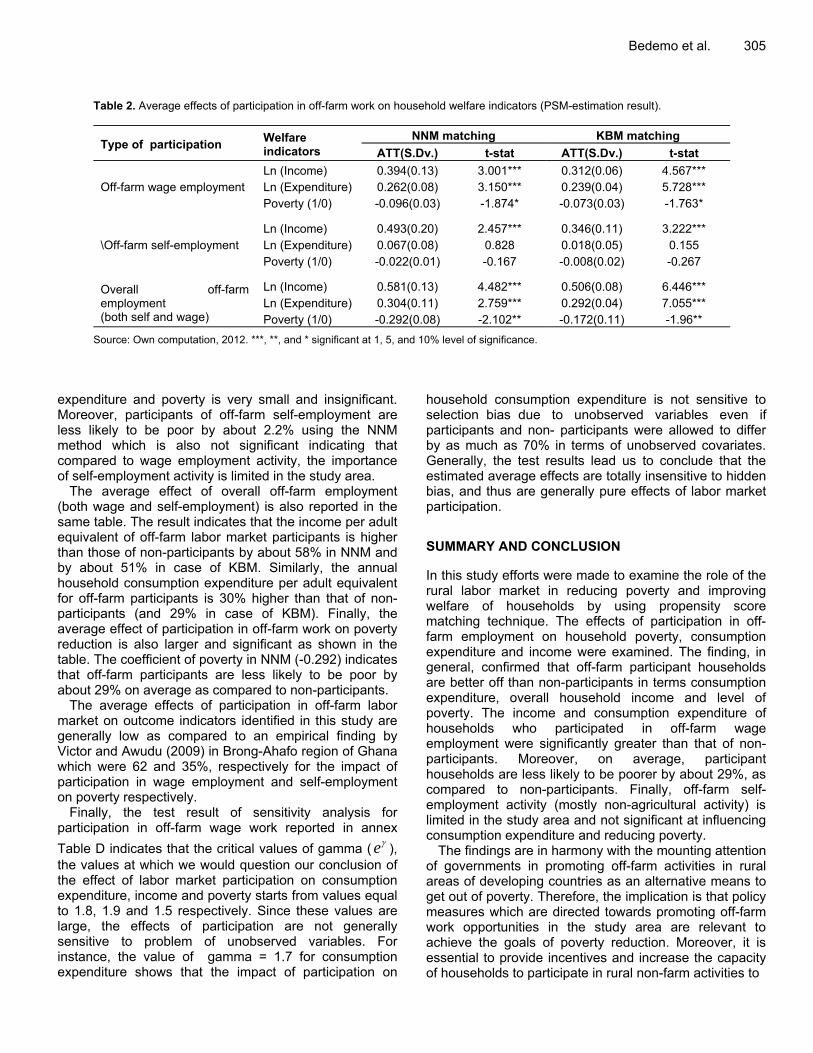
Bedemo et al. 305
Table 2. Average effects of participation in off-farm work on household welfare indicators (PSM-estimation result).
Type of participation Welfare indicators
NNM matching KBM matching
ATT(S.Dv.) t-stat ATT(S.Dv.) t-stat
Off-farm wage employment Ln (Income) 0.394(0.13) 3.001*** 0.312(0.06) 4.567*** Ln (Expenditure) 0.262(0.08) 3.150*** 0.239(0.04) 5.728*** Poverty (1/0) -0.096(0.03) -1.874* -0.073(0.03) -1.763*
\Off-farm self-employment Ln (Income) 0.493(0.20) 2.457*** 0.346(0.11) 3.222*** Ln (Expenditure) 0.067(0.08) 0.828 0.018(0.05) 0.155 Poverty (1/0) -0.022(0.01) -0.167 -0.008(0.02) -0.267
Overall off-farm employment (both self and wage)
Ln (Income) 0.581(0.13) 4.482*** 0.506(0.08) 6.446*** Ln (Expenditure) 0.304(0.11) 2.759*** 0.292(0.04) 7.055*** Poverty (1/0) -0.292(0.08) -2.102** -0.172(0.11) -1.96**
Source: Own computation, 2012. ***, **, and * significant at 1, 5, and 10% level of significance. expenditure and poverty is very small and insignificant. Moreover, participants of off-farm self-employment are less likely to be poor by about 2.2% using the NNM method which is also not significant indicating that compared to wage employment activity, the importance of self-employment activity is limited in the study area.
The average effect of overall off-farm employment (both wage and self-employment) is also reported in the same table. The result indicates that the income per adult equivalent of off-farm labor market participants is higher than those of non-participants by about 58% in NNM and by about 51% in case of KBM. Similarly, the annual household consumption expenditure per adult equivalent for off-farm participants is 30% higher than that of non-participants (and 29% in case of KBM). Finally, the average effect of participation in off-farm work on poverty reduction is also larger and significant as shown in the table. The coefficient of poverty in NNM (-0.292) indicates that off-farm participants are less likely to be poor by about 29% on average as compared to non-participants.
The average effects of participation in off-farm labor market on outcome indicators identified in this study are generally low as compared to an empirical finding by Victor and Awudu (2009) in Brong-Ahafo region of Ghana which were 62 and 35%, respectively for the impact of participation in wage employment and self-employment on poverty respectively.
Finally, the test result of sensitivity analysis for participation in off-farm wage work reported in annex
Table D indicates that the critical values of gamma (e ),
the values at which we would question our conclusion of the effect of labor market participation on consumption expenditure, income and poverty starts from values equal to 1.8, 1.9 and 1.5 respectively. Since these values are large, the effects of participation are not generally sensitive to problem of unobserved variables. For instance, the value of gamma = 1.7 for consumption expenditure shows that the impact of participation on
household consumption expenditure is not sensitive to selection bias due to unobserved variables even if participants and non- participants were allowed to differ by as much as 70% in terms of unobserved covariates. Generally, the test results lead us to conclude that the estimated average effects are totally insensitive to hidden bias, and thus are generally pure effects of labor market participation. SUMMARY AND CONCLUSION In this study efforts were made to examine the role of the rural labor market in reducing poverty and improving welfare of households by using propensity score matching technique. The effects of participation in off-farm employment on household poverty, consumption expenditure and income were examined. The finding, in general, confirmed that off-farm participant households are better off than non-participants in terms consumption expenditure, overall household income and level of poverty. The income and consumption expenditure of households who participated in off-farm wage employment were significantly greater than that of non-participants. Moreover, on average, participant households are less likely to be poorer by about 29%, as compared to non-participants. Finally, off-farm self-employment activity (mostly non-agricultural activity) is limited in the study area and not significant at influencing consumption expenditure and reducing poverty.
The findings are in harmony with the mounting attention of governments in promoting off-farm activities in rural areas of developing countries as an alternative means to get out of poverty. Therefore, the implication is that policy measures which are directed towards promoting off-farm work opportunities in the study area are relevant to achieve the goals of poverty reduction. Moreover, it is essential to provide incentives and increase the capacity of households to participate in rural non-farm activities to

306 J. Dev. Agric. Econ. take advantage of such opportunities. Such intervention would help overcome some entry barriers to off-farm employment thereby promoting efficient functioning of the rural labor market in the study area. In addition to being one important source of income for rural farm households, off-farm employment could help smooth incomes, which in turn smoothens consumption over long periods of time. Conflict of Interests The author(s) have not declared any conflict of interests. ACKNOWLEDGEMENTS The author express their thanks to Haramaya University and Wollega University (both in Ethiopia) for the financial support they provided us to successfully complete the research; East Wollega Zone Office of Agriculture and Rural Development for facilitating the contact with the districts in the study area and with the development agents, and the development agents who helped in conducting the survey. REFERENCES Abadie A, Imbens G (2006). Large sample properties of matching
estimators for average treatment effects. Econometrica 74(1):235-267. http://dx.doi.org/10.1111/j.1468-0262.2006.00655.x
Awuor Z (2007). Agricultural growth, rural poverty and hunger in Africa. AAAE Conference Proceedings (2007) College of Agriculture and Veterinary Sciences Depart. Agric. Econ. Ghana. 465-468.
Barbara T, Sophia B, Alastair B (2012). Key Issues in Agricultural Labour Markets: A review of major studies and project reports on agriculture and rural labour markets. P. 20, February 2012. ISBN 978-94-6138-191-0.
Bardhan P, Udry C (1999). Development Microeconomics. Oxford University Press Inc., New York. http://dx.doi.org/10.1093/0198773714.001.0001
Bernardin S (2012). Non-farm income diversification in rural Ghana: Patterns and determinants. Afr. Dev. Rev 24(3):233-244. http://dx.doi.org/10.1111/j.1467-8268.2012.00322.x
Blundell R, Dearden L, Sianesi B (2005). Evaluating the impact of education on earnings in the UK: models, methods and results from the NCDS. J. Roy. Stat. Soc. 168(3):473-512. http://dx.doi.org/10.1111/j.1467-985X.2004.00360.x
Bryson A, Dorsett R, Purdon S (2002). The use of propensity score matching in the evaluation of active labour market policies. Working paper number 4, London: Policy studies institute and national centre for social research.
Caliendo M, Kopeinig S (2008). Some practical guidance for implementation of propensity scores matching. J. Econ. Surveys. 22(1):31-72. http://dx.doi.org/10.1111/j.1467-6419.2007.00527.x
Carlos O (2010). Rural inequality, wage employment and labour market formation in Africa: Historical and micro-level evidence. Working Policy Integration Department International Labour Office, Geneva. P. 97.
David S (2010). The rural non-farm economy, livelihood strategies and household welfare. Afr. J. Agri. Res. 4(1):82-109.
Ellis F (2001). Rural livelihoods, diversity and poverty reduction policies: Uganda, Tanzania, Malawi and Kenya. Ladder Working P. 1.
Emmanuel E (2011). Rural livelihood diversification and agricultural household welfare in Ghana. J. Dev. Agric. Econ. 3(7):325-334.
Fydess K, Pamela J, Shively G, Dick S (2011). Income, poverty and
charcoal production in Uganda. Forest Policy. Econ. 13(2011):199-205. http://dx.doi.org/10.1016/j.forpol.2010.11.002
Haggblade S, Hazell P, Reardon T (2010). The Rural Non-farm Economy: Prospects for Growth and Poverty Reduction. World Dev. 38(10):1429-1441. http://dx.doi.org/10.1016/j.worlddev.2009.06.008
Imbens G (2004). Nonparametric estimation of average treatment effects under exogeneity. Rev. Econ. Stat. 86(1):4-29. http://dx.doi.org/10.1162/003465304323023651
Jayne T, David M, Mghen E (2010). Principal Challenges Confronting Smallholder Agriculture in Sub-Saharan Africa. World Dev. (38)10:1384-1398. http://dx.doi.org/10.1016/j.worlddev.2010.06.002
Kwadwo A, Samson J (2012). Increasing agricultural productivity and enhancing food security in Africa: New Challenges and Opportunities. Synopsis of an International Conference. International Food Policy Research Institute, Washington, DC, March 2012.
Leavy J, White H (2003). Rural labor markets and poverty in Sub-Saharan Africa. Working Paper, Brighton, Institute of Development Studies, University of Sussex.
Mariapia M (2007). Agricultural technology adoption and poverty reduction: A propensity-score matching analysis for rural Bangladesh. Food Pol. 32:372-393. http://dx.doi.org/10.1016/j.foodpol.2006.07.003
Mazumdar D (1989). Microeconomic issues of labour markets in developing countries; analysis and policy implications. Economic Development Institute of the World Bank. http://dx.doi.org/10.1596/0-8213-1183-2
Menale K, Bekele S, Geoffrey M (2010). Adoption and Impact of Improved Groundnut Varieties on Rural Poverty. Evidence from Rural Uganda. Discussion Paper Series May 2010, EfD DP 10-11.
Micevska M, Rahut D (2008). Rural non-farm employment and incomes in the Himalayas. Econ. Dev. Cul. Change 57(1):163-193. http://dx.doi.org/10.1086/590460
MoFED (Ministry of Finance and Economic Development-Ethiopia) (2012). Ethiopia’s Progress towards Eradicating Poverty: An Interim Report on Poverty Analysis Study (2010/2011). March 2012, Addis Ababa, Ethiopia.
Mulat D, Fantu G, Tadele F (2006). Towards a more employment-intensive and pro-poor economic growth in Ethiopia: Issues in Employment and Poverty. Discussion Employment Strategy Department, International Labour Office, Geneva. P. 22.
Otusu K, Yamano T (2006). The role of rural labor markets in poverty reduction: Evidence from Asia and East Africa. FASID discussion series on international development strategies 2006-12-007.
Rosenbaum P (2002). Observational Studies. New York, NY: Springer. http://dx.doi.org/10.1007/978-1-4757-3692-2
Rosenbaum P, Rubin D (1983). The central role of the propensity score in observational studies for causal effects. Biometrika. 70(1):41-55. http://dx.doi.org/10.1093/biomet/70.1.41
Sianesi B (2004). An evaluation of the Swedish system of active labor market programmes in the 1990s. Rev. Econ. Stat. 86(1):133-155. http://dx.doi.org/10.1162/003465304323023723
Sosina B, Barrett C, Holden S (2012). Does the nonfarm economy offer pathways for upward mobility? Evidence from a panel data study in Ethiopia. World Dev. 40(8):1634-1646. http://dx.doi.org/10.1016/j.worlddev.2012.04.019
Tanguy B, Eleni G, Alemayehu S (2007). Smallholders’ commercialization through cooperatives: A Diagnostic for Ethiopia. IFPRI Discussion P 00722
Verner D (2006). Labor markets and income generation in rural Argentina. World Bank Policy Research Working P. 4095. http://dx.doi.org/10.1596/1813-9450-4096 http://dx.doi.org/10.1596/1813-9450-4095
Victor O, Awudu A (2009). Non-farm employment and poverty reduction in rural Ghana: A propensity-score matching analysis. Paper prepared at the International Association of Agricultural Economists conference, Beijing, China, August 16-22.
World Bank (2008). World Development Report 2008: Agriculture for Development Washington, DC.
Wooldridge J (2002). Econometric Analysis of Cross Section and Panel Data. The MIT Press, Cambridge.

Bedemo et al. 307 ANNEX
Table A. Logit estimation result (for predicting the propensity scores) [Dependent variable: Participation in off-farm work (1/0)].
Explanatory variable
Participation
Wage work Self-employment Overall off-farm work
Coef. St.Er Coef. St.Er Coef. St.Er
Age in years 0.024*** 0.011 -0.140 0.112 -0.102 0.095 Age square -0.001*** 0.0005 0.002 0.001 0.001 0.001 Education level of the head 0.045 0.055 -0.051 0.064 0.032 0.064 Gender(1=male;0 = female) 0.618*** 0.243 0.357** 0.172 0.337*** 0.149 Adult laborers(aged 15-64) 0.387** 0.201 0.056 0.036 0.213* 0.130 Elder children(aged 10-14) 0.127 0.259 0.145** 0.075 0.086* 0.044 Dependents -0.262** 0.126 -0.075 0.153 -0.366** 0.153 Land cultivated in hectares -1.524*** 0.471 -0.101 0.476 -1.007*** 0.315 Amount of credit obtained -0.076 0.052 0.041*** 0.008 0.023*** 0.007 Animal wealth in TLU 0.250 0.214 -0.065 0.048 -0.012 0.009 Non-labor income -0.054 0.062 -0.001 0.0007 0.004 0.005 Distance in kms 0.061* 0.035 -0.010 0.041 0.047 0.042 Dummy for Guto Gida 0.343* 0.177 0.083 0.069 0.237** 0.111 Dummy for Jima Arjo 0.169* 0.092 0.120 0.099 0.167* 0.102 Constant -2.160 2.629 -1.408 0.926 2.285 1.344 Pseudo R2 0.29 0.20 0.37 LR chi2 128.6 37.01 193.44 Log likelihood -160.1 -122.4 -114.0 Prob> chi2 0.000 0.052 0.000
Source: Own calculations, 2012. ***, **, and * significant at 1, 5, and 10% level of significance.
Table B. Covariate balancing before and after matching (for participation in wage work).
Variable name Sample Mean Reduction t-test
Treated Control % Bias %|Bias| t p>|t|
Age Unmatched 40.524 38.641 17.8 1.60 0.089 Matched 39.582 38.563 7.6 57.3 0.75 0.451
Year of schooling of head Unmatched 4.321 5.218 -24.4 -2.20 0.029 Matched 4.546 5.214 -18.2 25.5 -1.33 0.183
Average family schooling Unmatched 0.708 0.732 -9.2 -0.82 0.411 Matched 0.711 0.731 -7.6 16.8 -0.58 0.565
Gender (1= male) Unmatched 0.976 0.981 -3.1 -0.28 0.778 Matched 0.964 0.980 -11.3 -260.1 -0.84 0.400
Number of adult labourers Unmatched 4.214 3.968 14.5 1.90 0.083 Matched 4.146 3.945 11.8 18.7 0.90 0.369
Number of young children aged1015
Unmatched 1.191 1.218 -2.6 -0.23 0.817 Matched 1.273 1.198 7.0 -173.2 0.50 0.620
Number of dependents Unmatched 2.869 3.237 -20.6 -1.85 0.065 Matched 3.327 3.208 6.7 67.7 0.49 0.628
Land cultivated in adult equivalent
Unmatched 0.465 0.660 -51.4 -4.65 0.000 Matched 0.463 0.578 -66.6 -29.6 -1.63 0.094

308 J. Dev. Agric. Econ.
Table B Contd.
Non-labour income Unmatched 287.32 144.04 20.3 1.82 0.070 Matched 258.36 141.06 16.6 18.1 1.35 0.176
Animal wealth in TLU Unmatched 5.384 5.487 -2.6 -0.24 0.812 Matched 4.803 5.477 -17.4 -556.1 -1.23 0.218
Credit Unmatched 309.6 333.20 -2.9 -0.26 0.792 Matched 132.6 348.12 -26.7 -813.2 -1.86 0.103
Distance to the nearest market in kms.
Unmatched 5.049 4.525 12.3 1.11 0.270 Matched 4.318 4.466 -3.5 71.8 -0.26 0.794
Source: Own calculation using survey data, 2012. Table C. Additional indicators of matching quality.
Type of off-farm participation
Pseudo R2
before matching Pseudo R2
after matching LR χ2(p-value)
before matching LR χ2(p-value) after matching
Total % mean standardize bias reduction
Total off-farm work 0.371 0.057 193.44(0.000) 9.57 (0.793) 87.72 Wage work 0.287 0.042 128.57(0.000) 24.15 (0.256) 84.84 Self-employment 0.197 0.036 37.01(0.052) 13.56(0.631) 84.33
Source: Own calculation using survey data, 2012.
Table D. Sensitivity analysis test for hidden bias (for participation in wage work).
Gamma ( e ) Income Consumption expenditure Poverty
p-value p-value p-value
1.0 0.004 0.0001 0.007 1.1 0.008 0.004 0.016 1.2 0.015 0.012 0.041 1.3 0.027 0.022 0.069 1.4 0.036 0.037 0.099 1.5 0.049 0.057 0.134 1.6 0.064 0.078 0.174 1.7 0.081 0.096 0.219 1.8 0.092 0.125 0.268 1.9 0.113 0.154 0.339 2.0 0.168 0.196 0.372 2.1 0.212 0.247 0.429
Source: Own calculation using survey data, 2012.
Vol. 6(7), pp. 309-317, July, 2014 DOI: 10.5897/JDAE2014.0571 Article number: 1326B2645623 ISSN 2006-9774 Copyright © 2014 Author(s) retain the copyright of this article http://www.academicjournals.org/JDAE
Journal of Development and Agricultural Economics
Full Length Research Paper
The livelihood effects of landless people through communal hillside conservation in Tigray
Region, Ethiopia
Melaku Berhe1* and Dana Hoag2
1 Department of Resource Economics, Agricultural Extension and Development, College of Dryland Agriculture and Natural Resources, Mekelle University, P.O.Box 231, Mekelle, Ethiopia.
2Department of Agricultural and Resource Economics, Colorado State University, Fort Collins, CO 80523-1172, USA.
Received 27 March, 2014; Accepted 30 April, 2014
In the Tigray region of northern Ethiopia, landless people contributed to the existing land degradation by exploiting the economic possibilities of natural resources from communal hillside areas. This has been practically observed in the area that the landless people have been depending on the available natural resources to supplement their means of living through sales of timber, fire-wood and charcoal. To address this problem, the Tigray Regional State has distributed denuded hillside areas to the landless people. It was believed that renovating bared mountain hillsides through conservation practices could serve as a means to create livelihood sources for the landless poor. This study has been inspired to investigate whether the introduction of communal hillside distribution to the landless people has resulted in livelihood and environmental improvements in the Tigray Regional State. Six districts were randomly selected namely; Kola-Tembien, Hintalo-Wejerat, Kilte-Awlalo, Degua-Tembien, Alaje and Ofla which all represented by 450 sampled respondents (418 males and 32 females). The respondents were interviewed using semi-structured questionnaires including ideas from group discussants and key informants. Results revealed that landless in all the districts applied conservation methods mainly of stone bund, trench and tree plantation. Their main livelihood sources using the hillside areas were; production of honey, fruits, livestock products, timber, vegetables, fuel-wood and animal fodder. Estimated results further indicated that supporting services given by forest experts and local authorities, credit access, membership in the village development committee, respondents’ perception to land degradation and their educational levels were the major inducing factors that affect landless people to participate in hillside conservation. Key words: Conservation, degradation, hillsides, landless, livelihood, sustainable, people.
INTRODUCTION At global level, natural resource degradation on mountains slopes is widely believed to be one of the causes of environmental damage that expedites the
adverse effects of climate change. The increased effect of this degradation coupled with climate change (Sanchez and Leakey, 1997; Havstad et al., 2007)
Corresponding author. E-mail: [email protected], Tel: +251914782072. Fax: +25234409314. Author(s) agree that this article remain permanently open access under the terms of the Creative Commons Attribution License 4.0 International License

310 J. Dev. Agric. Econ. has led to the decline in agricultural productivity in the Global South. The consequent loss in land productivity results in global economic and social crisis that is the dominant threat to the security and well-being of populations of most countries of the Global South (Fitsum et al., 1999; Hengsdijk et al., 2005; Atakilte et al., 2006). As much of the sources of land damage have prevailed on steep communal hillside areas and the available resources are fully accessible to the advantage of everyone, the issues of environmental management have become priority concerns in these countries (Gebremedhin et al., 2003). Cognizance of resource mismanagement due to the presence of externalities arising from communal resource overutilization, two collective action theories proposed by Hardin (1968) and Ostrom (1990) have developed over time. The mantra of each theory is based on the existing common resource challenges and thus it seems reasonable to view the analysis of this study in light of both theories.
From the time that Hardin (1968) published his article “The Tragedy of the Commons”, many scholars understood that communal resources were often severely exposed to maximum overexploitation by free riders within any given community. For Hardin, it was assumed that individuals proceed to satisfy their self-interest by over utilizing the common resources with no regard for others, which would eventually damage the communal resource bases (Hardin, 1968; Welch, 1983). Their underpinning proposition was based on the absence of individual incentives to utilize communal resources in efficient ways. According to this theory, common pool resources can be managed through central stewardship either by a government or through privatization. The reason cited for this is that individual incentives evolving from numerous benefits are associated with property rights over long term, and thus privately owned resources are more sustainable than publicly owned resources.
An increasing number of scholars oppose Hardin’s theory and base their reasons for their opinion that the source of the problems highlighted in ‘tragedy of the commons’ did not originate from the failure of common property ownership, but rather from institutional and policy failures to manage communal resources, nor the individual’s mismanagement to enforce internal decisions for collective actions at communal level (Ostrom, 1990; Beaumont and Walker, 1996; Poteete and Ostrom, 2000; Forsyth, 2006). These scholars conceived that decentralized collective management of common property resources by users could be an appropriate system for overrating the ‘tragedy of the commons’ (Agrawal, 2001; Ostrom, 2008). As viewed by Trivers (1971), the tragedy of commons can be solved via people’s dedication to manage communal resources altogether. As people exist within social bonds, they interact closely, including experience sharing among each, common cooperation against free-riders, and creation of local bylaws and binding regulations.
Furthermore, Axelrod and Hamilton (1981) contended that relationships among people usually strengthened due to their learning behaviour for cooperation in mutuality sense. In this sense, global environmental damages can be addressed via international collective actions (Ostrom, 2008).
The above debates over how communal resources can compatibly be governed by local community and which approach can plausibly be applicable for renovating the denuded resources have been studied widely. However, there is scant information on distributed mountainous hillside areas and how landless people utilize communal hillside resources and how the resources can be brought back into their natural green scenery. Such similar cases are apparently observed in the Tigray region of northern Ethiopia where land degradation is the major reason for low level of land productivity and devoid of vegetation (Hengsdijk et al., 2005; Wolde et al., 2007). Many landless people depended on the remnants of communal hillside forest patches by selling fire-wood and charcoal, timbering, traditional mining, cutting tree branches and herbaceous woods to feed their animals. This has further spirally escalated the ill-effects of land degradation (Hurni et al., 2005; Carolyn and Asenso, 2011). Due to their dependency on communal forest patches, lot of erosion is taking place and the areas are getting degraded year by year. In the upper catchment hillside mountain areas where many people cut-down live trees for firewood and charcoal sales, the position of forestland is being further exposed to severe land degradation (Badege, 2009). In other land areas in which mining and logging of trees have been taking place, large trees are almost lost, only bushes and stony degraded areas can be seen. At present, big trees can be observed only near to churches and mosques.
The increasing problem of landlessness in the areas has put pressure on the local administrators to rethink about the sustainable use of non-arable hillside mountains. The strategy designed was distributing the bared hillside areas to the landless people; after first establishing structures for soil and water conservation through community mobilization (Yifter et al., 2005; Carolyn and Asenso, 2011). Such hillside distribution to the landless poor started in 1999 in the Tigray region. As the result, landless people have conserved the areas by planting fruit trees, growing fodder for their cattle and engaging in honey production. The distribution of non-arable hillside areas to the landless people has two advantages; the areas which were previously found denuded are recently getting renovated, and, the landless people whose means of living previously depending on fuel-wood sales and traditional mining have started shifting to the production of fodder trees, fruits, vegetables, honey and commercial timber trees like eucalyptus.
However, those landless people who do not have access to other means of living are still dependent on the

hillside communal forests. Since they contributed to deforestation and land degradation, it is reasonable to address the problem by creating long-term linkages between livelihood sources and hillside conservation so as to enable the landless people to utilize the hillside areas in sustainable ways. In a community of having shortage of arable land like in the Tigray Region, linking hillside distribution to the landless people and conservation is crucial. Therefore, a clear understanding on the livelihood effects of landless people’s participation on hillside conservation is helpful in bringing long-lasting hillside renovation. In doing this, the objectives of the study were: (1) To examine perception of landless people on land degradation (2) To verify the contributions of chosen hillside rehabilitation activities to the livelihood of landless people. (3) To identify factors that affect the participation of landless people on hillside conservation MATERIALS AND METHODS Sampling design Field survey was done in the Tigray Regional State of northern Ethiopia during 1 April to 30 May, 2013. In the study area, many landless people were reaping benefits by practising hillside rehabilitation. Following Atakilte et al. (2006), the six research sites selected for this study were categorized on the basis of their agro-climatic classifications. Areas below 1500 m above sea level are considered as lowland (Quola), areas situated at 1500 to 2300 m above sea level are medium altitude (Weina-Degua); and the areas over 2300 m above sea level are highland (Degua). Based on these classifications, Quola-Tembien is located at an altitude of 800 to 1500 m above sea level in a lowland district. While Degua-Tembien (midland) is situated at an altitude of 1200 to 2100 m above sea level, Kilte-Awlalo and Hintalo-Wejerat (midland) are found at an altitude of 1500 to 2540 m above sea level. The high land areas of Alaje and Korem are also positioned with a proxy altitude range of 2300 to 3140 m above sea level.
Across all climatic zones, the Tigray Regional government is the first region that has undertaken distribution of bared communal hillside areas to landless people to enable them access to various livelihood sources in a sustainable way. In Tigray region, there are 35 woredas (districts) that have distributed non-arable hillside areas to the landless people. During sampling, criteria were used so as to distinctively identify the districts that have fully practised the hillside rehabilitation from those did not. They were: (1) Districts that distributed hillside areas to landless people (2) The presence of landless people whose livelihood sources depend on the conserved and improved hillside areas (3) Landless people who have got training regarding hillside rehabilitation. Six districts that have fulfilled the criteria were selected and the survey was conducted across three stratified agro ecological zones (lowland, midland and highland). From each agro ecological zone, individual sample representatives were selected using simple random sampling technique. Following Chand et al. (2012), the
Berhe and Hoag 311 required sample size was estimated at 99% confidence level and below 1% error commitment as shown below:
)1(.
)1(2
2
PPZeN
PPNZn
Where: n = is the sample size, N = is the population size, Z= Confidence level at 99%, Z=2.57, P= Estimated population proportion (0.5), e = is the error level (0.003).
Based on the sampling estimation made out of the total 1808 population size, the required sample size was 450. Doing a proportionate stratification from the total 1679 males and 129 females, the representative sampled households were 418 males and 32 females drawn from each of the three agro ecological zone (117 from lowland, 166 from midland and 167 from highland) as shown in Table 1. Data sources and collection This study was based on data obtained from both secondary and primary sources. Due to the wide ranging implications of the involvement of landless people into hillside conservation to generate their income, primary data were broadly collected by mixing both qualitative and quantitative methods. The following methodological approaches were employed to address the objectives. In order to bring together logical information addressing the research objectives, eight key informants were taken. The selection of the key informants was based on their experiences, better technical knowledge on hillside conservation, representatives of both men and women landless people and village leaders drawn from each district. In the presence of the chosen discussants, the whole thing was open for discussion and the informants were participating to criticize, correct, or point out, and answer in any way based on the context of their villages. The eight key informants participated in the in-depth interviews were: animal expert, two experienced farmers (a male and a female), forest expert, representative elder, leader of Farmers’ Association, Women’s Association and leader of development committee. Dependent and independent variables Dependent variable The dependent variables are two consecutive hillside conservation actions. The first one is participation of landless people on hillside conservation and the next one is the amount of conservation done by the landless people, measured in meters of stone/soil bund. Independent variables Some of the independent variables are: income sources from the hillside areas, (household demographics such as gender, age, education, marital status of household head), active family size, value of livelihood assets gained from the hillside rehabilitation, cattle size, land size in the hillside, non-cattle tropical livestock unit, access to water sources, cost of conservation, cost on water use, new hillside conservation strategies, conservation methods, source of information, experience in hillside conservation, contact with extension agents, member of farmers association, satisfaction with improved tree varieties, access to off-farm activities, location of the hillside area, hillside income, non-hillside income, etc).

312 J. Dev. Agric. Econ.
Table 1. Sample frame of the respondents.
Agroecological zone Sex Population Sample
Lowland Females 29 8 Males 403 109 Total 432 117
Midland Females 60 15 Males 844 151 Total 904 166
Highland Females 40 9 Males 431 158 Total 464 167
Total Females 128 32 Males 1680 167 Total 1808 450
Data analyses Both qualitative and quantitative data analyses methods were applied. Qualitative data analysis was carried out to capture information that was collected from key informant interviews, household surveys, and direct observations. As the project uses a mix of methods to understand the richness and complexity of the hillside conservation and their effects on the benefits of landless people, data triangulation was used to analyse, validate and verify the results. During triangulation, the results from different methods of qualitative and quantitative information were compared to strengthen the outcome of the project. To analyse the linkages between livelihood sources obtained from the hillside areas and the role of the landless people on hillside conservation, descriptive statistics such as measures of central tendency and dispersion were employed. The strength and direction of relationships between different selected dependent and independent variables were examined using statistical tests like chi-square to look at the associations between discrete variables and t-tests to compare the mean differences between continuous variables. Econometrics techniques To identify various factors that influence the involvement of landless people on hillside conservation the two-stage Heckman model was applied. Conservation activities can be influenced by various explanatory factors. Some of these factors can be household-behaviours, income levels and sources, resource availabilities, land management and institutional variables. In this view, it is possible to analyse the different factors that instigate landless people to participate in environmental rehabilitation. Households in the study areas undertake two decisions (such as decision of participation in hillside conservation and construct some amount of stone-bunds, trench, tree plantations, and others in the hill-side areas) as the activity provides them a certain threshold level of utility in terms of yield gained from the improved hillsides after rehabilitation, (fodder, honey or fruit produce or commercial trees).
The choice that the landless people have to make is based on the unobserved utility obtained from participation in those activities. These kinds of choice models assume that an individual household’s choice is the result of his/her preference (Wooldridge, 2002). In such a scenario, some of the factors that influence the behaviour of landless people in conservation participation activities
may also influence their performances on the level of conservation or produce using the hillside. Analytical estimation of the outcome equation (hillside conservation in meters) alone would be, therefore, biased in the presence of sample selection. Sample selection may occur as a result of self-selection by research units (observation units – landless people in this case). The resulting bias (sample selection bias) emanates from the correlation between the error term and independent variables (Heckman, 1979; Verbeek, 2004). All these problems basically may arise from endogenous relationships among variables, measurement error of variables and missing cases of variables. Hence, the selection equation in the first stage of the Heckman two-stage model is accountable to capture factors affecting participation decision made by the landless people. This equation is used to construct a selectivity term known as the ‘Inverse Mills ratio’ which is added to the second stage ‘outcome’ equation’ so as to explain factors affecting hillside conservation measured in meters. The inverse Mill’s ratio is a variable for controlling bias due to sample selection (Heckman, 1979). The second stage involves including the Mills ratio to the amount of hillside conservation to be measured in meters and estimating the equation using Ordinary Least Square (OLS). Moreover, with the inclusion of extra term (inverse Mill’s ratio) into the second stage, the coefficient in the second stage ‘selectivity corrected’ equation becomes to be unbiased (Wooldrige, 2002; Verbeek, 2004). Specification of the Heckman two-step procedure, which is written in terms of the probability of landless people to participate in hillside conservation, is given as follows:
0*i
z if 0i
z
0*i
z if 1i
ziε
ix
iθ*
iz
EquationSelection
(1)
equationsboth for n) …3 2, 1, = (i Where
0i
z if observednot is i
y
1i
z if i
y*i
yi
*
EquationOutcome
uiviiy
(2)

Berhe and Hoag 313
Table 2. Socio-economic characteristics of the landless people.
Socio-economic characteristics of landless people Mean Minimum MaximumAge in years 40.9 20 68 Experience in years 7.4 3 12 Cattle Holding (cows and oxen) 2.5 1 7 Family size 2.8 1 6 Net gain in Birr annually 783.3 20 2330
In this case, the amount of hillside conservation measured in meters represented by Equation (2) becomes the outcome equation- the variable on which we are interested to see the effect of various factors and the income gained from the hillsides. Equation (1) represents the decision for the participation activities of the landless people become the selection (precondition) equation. The overall selection model indicates that the extent of
hillside conservation (*iy
) is observed when a given landless household (i) participates in conservation activities, that is, zi= 1. In the given model, in Equations (1) and (2), sample selection occurs when the correlation between the error terms of the two models, corr(εi , ui) = ρ, is different from zero, assuming that the error terms εi and ui are jointly normally distributed, independently of xi and vi , with zero expectations. Both xi and vi are the vectors of independent variables that affect the participation of landless households on hillside conservation. In the presence of the selection bias, typical models such as probit models are inefficient and OLS estimation is biased (Verbeek, 2004). Thus, the implication is that the selection problem should be corrected and we need a superior estimator for this. Based upon the specification of the dependent variable of the outcome equation, the two-step Heckman selection model is appropriate. RESULTS AND DICUSSION Socio-economic characteristics of respondents According to the criteria profoundedly categorized by Jacobsen (1999), the age between 15-64 years was active labour force population, whereas people whose age less are than 15 years and the older people whose ages exceeding 64 years were grouped as economically passive and dependent. Following this, the results shown in Table 2 indicate that the mean age of the sample respondents was found to be about 41 years; implying the involvement of the landless people mainly from the active labor force group. Out of the total 450 interviewed respondents, male landless people were 418 and females were 32. Based on additional ideas obtained from the key informants and group discussants, the females in these areas were dominantly burdened with indoor family management tasks and cultural stereotypes which hindered their participation in hillside conservation to support their own livelihood.
This finding has similarity with the studies made by Chala et al. (2012) and FAO (2012) in the sense that females in Ethiopia have cultural hindrances that obstructed their involvement in various developmental activities outside their home. It was found that women
were engaged in family management of daily house tasks such as cooking, washing and taking care of their children. In most cases, the men acted as the head of the household; in making money and satisfying the family demand. The survey result further revealed that the landless people in the study areas had an average experience of 7.4 years in hillside conservation with a minimum of 3 and maximum 12 years. Each respondent consisted of an average family size 2.8, and owned a mean number of cattle about 2.5 with a minimum 1 and maximum 7. The average annual net gain reaped by the respondents out of their participation in the hillside rehabilitation was estimated in Ethiopian Birr 783 with a minimum of 20 and maximum 2330. Perception of landless people and their particiaption on hillside conservation The landless people were asked to elucidate their perception towards the damages they imposed on the environment due to their dependence for fire-wood and charcoal sales by exploiting the remnant forest areas. The key informants and group discussants reported that degradation on hillside areas was perceived as a problem hindering livelihood improvement and agricultural productivity in the study areas. The data gathered from the field survey further confirmed that the landless people sensitized the exisitng damages they were imposing on the environment such as charcoal and fire-wood extraction. About 95% of the interviewed landless people witnessed that the severity of land degradation in the area was getting worsened year to year. These respondents largely examined the incidence of land degradation predominantly occurred in denuded mountain hillside areas. Of the landless people who reported the problems of land degradation in the hillside areas, more than 86% admitted that their dependence on the mountain hillsides accelerated the damages. The remaining 5% of the respondents did not notice the prevalence of land degradation in the hillside areas (Table 3).
Table 4 depicts the summary of hillside conservation done by the landless people all over the six woredas (districts). The landless households participated in conservation activities of soil bund, stone bund, tree plantation and a mix of trench and bunds to rehabilitate

314 J. Dev. Agric. Econ.
Table 3. Perception of landless people on land degradation.
Perceive land damages Worsened No Change Improved
Frequency 427 15 8 Percentage 95 3.3 1.7
Table 4. Summary of hillside conservation done by the landless people.
Conservation methods Observation Mean Std. Dev. Min. Max.
Soil/Stone bund in meters 421 111.5 51.3 32 196 Trench (in meter square) 450 22 9.5 0 53 Tree plantation (Number) 402 36 19.2 6 81 Mix of trench and stone bund 356 72 44.3 86 108
Table 5. Ways to achieve livelihoods of landless people using hillside conservation by woredas (Districts).
Income Sources Woredas (Districts)
Alaje Hintalo-wejerat
Degua-Tembien
Kilte-Awlalo
Quola-Tembien
Ofla Frequency Percent
Sale of timber/Fodder 3 14 4 11 7 7 46 10.2 Sales of vegetables 5 15 7 7 5 3 42 9.3 Sale of honey 12 22 14 37 10 22 117 26 Livestock 8 26 10 28 10 20 102 22.7 Sale of fuel-wood 7 16 5 16 7 11 62 13.8 Others 8 24 5 18 11 15 81 18 Percent 9.6 26 10 26.5 10.5 17.3 100 100
the hillside areas. On average, about 111.5 m of soil/stone bund was implemented by the landless people. The average number of trees planted by the landless people was about 36. Some efforts made by the landless households to implement conservation practices using trench was accounted for 22 m2 during the year 2012/2013. Applying different types of conservation methods, the landless people in the area were to rehabilitate the denuded hillside areas from which they generated their income sustainably. The amount of soil and water conservation done in the hillside areas indicates that the landless people who have obtained land grants did not perform sufficient hillside conservation as compared to the hillside areas given to them. Group discussants mentioned that the large portion of the hillside areas distributed to the landless people has not yet been conserved. Another study done by Gebremedhin et al. (2003) similarly found that in the Tigray Regional State, various conservation measures have been carried out by community mobilization mainly of stone terraces and bunds, micro-dams, trenches, tree planting, area enclosures, regulations for grazing lands, control of burning and applications of natural fertilizers like manure and compost.
Contributions of chosen hillside conservation to the livelihoods of the landless poor Table 5 illustrates the major ways through which the landless people pursued to improve their livelihoods by applying various hillside conservation methods. There is a potential for improving the livelihoods of the landless people by restoring the degraded hillside areas through their participation in various conservation methods. As the result of their participation, various income sources were created by the use of hillside areas. Out of the total income, the portion obtained from the sales of honey accounted for 26%. This was followed by 22.7% of the income share generated from the livestock products. Using the hillside areas, about 10.2% of the total income was reaped from sales of timber like commercial eucalyptus trees, and 9.3% was from sales of vegetables. While the landless people still continue to generate 13.8% of the total income sources from the sales of fire-wood and charcoal, the remaining 18% was from other income sources such as daily labour wage, pity business, poultry and sales of fodder. It is indicated in the figures that different livelihood sources have served the landless people as sources of additional income to supplement

Berhe and Hoag 315
Table 6. Total Annual Gain in Birr from the Hillsides by Agro-ecology.
Agro-ecology Summary of Income from the Hillside Rehabilitation in Ethiopian Birr
Frequency Mean Standard Deviation Minimum Maximum
Lowland 117 778.2 436.1 32 2107 Midland 166 772.8 478.5 26 2327 Highland 167 797.2 433.6 20 2318
Table 7. Participation of landless people on hillside conservation using heckman regression.
Explanatory variables Soil/Stone-bund
Explanatory variables Soil/Stone-bund
Coefficient P-Value Coefficient P-Value
Tree satisfy 1.056088 0.646 Religious leader -4.461652 0.700 Benefit hillside -2.763954 0.311 Social committee .2037514 0.956 Experience 3.842082 0.323 Village justice -17.01396 0.291 Absence of demarcation -8.161377 0.122 Perceived degradation 24.37742 0.000*** Dummy advice 6.878082 0.021** Farm size 4.426882 0.215 dummy extension 4.436521 0.007*** education -7.33115 0.001*** age -.5748796 0.057 credit 8.600637 0.000*** seedlings .2487836 0.054 _cons 133.3123 0.000 Development committee 5.945144 0.047**
Note that *** and ** are significant at 1 and 5% respectively. their means of living. Sales of honey and livestock played a considerable role in supplementing the landless people with additional incomes.
The proportion of fuel-wood comprising both charcoal and fire-wood (13.8%) serving as an income source for the landless people has important implication that about 62 landless people were found to be dependent on the natural resource forests. This may show how their dependency on the natural forests has imposed them to pursue on their short-term perspective, whereby they stick to deal with the immediate livelihood needs without considering the long-term effects of their actions on the natural resource base. This requires compatible intervention that can reshape the direction of the landless people towards honey production, commercial tree plantation, livestock rearing and vegetables which are eco-friendly livelihood alternative sources. In light of these findings, similar conclusions made by Habibah (2010) indicating that farmers can only be active participant in conserving natural resources if they find that it gives them any kind of perceived benefits. Hence, all the benefits from the hillside areas should be clearly categorized as environment friendly and non-friendly so that the landless people could be directed towards the sustainable pathways. The landless people whose income sources generated from the hillside areas in each woreda (district) is presented in Table 5. The income share of the landless people by districts as ways of their livelihood sources were: Quola Tembien (37.1%),
Hintalo-wejerat (26%), Ofla (17.3%), Degua-Tembien (10%) and Alaje (9.6).
The recorded annual income obtained by the landless people from the highland, midland and lowland agro-ecologies were on average 797.2, 772.8 and 778.2 birr, respectively (Table 6). The one way anova test revealed that there was no statistical and significance income differences among the three climatic zones. However, the big variations between the minimum and maximum income earnings in each agro-ecology indicates the need to intervene to narrow the disparities among the landless people. Factors that affect participation of landless people on hillside conservation Table 7 demonstrates the regression outputs of the two-stage Heckman Model to distinctively identify the major factors that induce the landless people to involve in hillside conservation. The coefficient of the inverse Mils ratio (lambda) using the Heckman first stage regression was statistically significant at 1% probability level (Prob > chi2 = 0.0000), indicating the presence of sample selection bias. After the correction of selection biases by including the inverse Mills ratio into the second stage of the Heckman model (OLS regression), the results were obtained as shown on Table 7.
Conservation was used as dependent variable which dominantly practiced by the farmers in the study area

316 J. Dev. Agric. Econ. such as soil and stone-bund measured in meters. Regressing the dependent variable soil/stone bund on the explanatory variables, the variables like extension services given by the agriculture experts (dummy extension), membership of the development committee in the village (Development committee), perceived land degradation (Perceived degradation), access to credit services (Credit) and educational level (education) are statistically significant at 1% probability level. The variable, dummy advice refers to support given to the landless people mainly from the local authorities which is statistically significant at 5% as shown in Table 7. It indicates that the more the landless people received advices from the forest experts and local leaders; they would be inspired to apply more meters of soil and stone bund in the mountainous hillsides. For instance, the landless people that received advice regarding hillside conservation implemented about 6.9 more meters than those did not receive the services, where the other intervening variables held constant.
The implication may be that the advisory service provided to the landless people is helpful in facilitating hillside conservation. This conforms to the view of Kashwan (2013) in the sense that development agents offer technical advices in conservation and bringing workable collaboration between the entire community and the forest users. Similarly, practical lessons and experiences disseminated by the forest experts and local leaders in the study areas hasten the action of the landless people through which the hillside areas have become livelihood sources for the landless people. This further encourages them to share responsibilities in hillside conservation along with the community which eventually leads to reduce social costs. Accordingly, the landless people and the community at large will have intimate knowledge in renovating the hillside areas sustainably and are able to monitor and protect the area from any threats.
The participation of the landless people at various development activities within the village is another important factor affecting the level of hillside conservation by the landless people. Hence, the landless people having exposure to participate as a village development committee (Development committee) tended to apply 5.9 more meters of soil and stone bund than the ordinary people. Their participation as a member of development committee in the village may broaden their awareness about the severity of land degradation. Hence, the landless people that perceived the existing land degradation (Perceived degradation) implemented more stone bunds of about 24.4 m than those did not perceive. With respect to educational level, the landless people having high level of years of schooling may tend to conserve their environment. But, the Two-Stage Heckman model regression output shows that additional one year schooling on average decreases the participation of the landless people by about 7 m of
stone and soil bunds in the hillsides (Table 7). The negative result indicates the decrease level for the landless people to participate in stone bund conservation. This was also supported by the key informants and group discussants in the sense that most of the landless people having higher level of education are assigned in various administration activities in the villages. In addition, some migrate to other places to search better income sources temporarily. CONCLUSIONS AND SUGGESTIONS Landless people have contributed to the existing land degradation by exploiting the economic possibilities of natural resources from the communal hillside areas. This has been practically observed in the hillside mountain areas from which landless people supplemented their livelihoods through sales of fire-wood and charcoal, timbering and fodder production, livestock rearing, growing fruit trees, and growing vegetable items. The study has been inspired to investigate whether the introduction of communal hillside distribution to the landless people has resulted in livelihood and environmental improvements in the Tigray Regional State. It was based to verify the idea that environmental rehabilitation in Tigray can be achieved via conservation of mountainous hillside areas with concurrent emphasis of supporting the livelihoods of the landless poor. The study revealed that landless people have tackled land degradation by applying various hillside conservation methods such as soil/stone bunds, trenches, tree plantation and zero grazing. However, lots of landless people have still relied on sales of fire-wood and charcoal to supplement their means of living. Besides, the people’ participation on hillside conservation was found to be insufficient due to several restraint factors. The Heckman two-step regression output indicated that collaborative advisory services from forest experts and local authorities (dummy advice), membership in the village development committee (Development committee), landless people’ perception on land degradation (Perceive degradation), extension services, credit accesses and educational levels are the major determinant factors that induce the landless people’ participation on hillside conservation to improve their livelihoods. Therefore, the following actions can possibly be sound to use hillside areas sustainably:
(i) Provision of continuous support from local leaders and development agents by instigating the landless people to involve on hillside land grants and undertaking extensive conservation to improve their livelihood bases. (ii) Build the capacity of the landless people through training, workshops, demonstrations, information dissemination, and experience sharing to increase their ability to utilize the hillside areas sustainably.

(iii) Enable the landless people to be fully detached from the sales of fire-wood and charcoal by providing substitutive income sources via communal hillside distributions. (iv) Identify trees compatible to each agro-ecology and cultivate the hillside areas with trees that can bear fruits, and serve for animal feed. (v) Plant bee forage, thereby increase honey yield with positive attitude for forest care and protection, which leads to sustainable job creation for landless people. Conflict of Interests The author(s) have not declared any conflict of interests. ACKNOWLEDGEMENTS Authors would like to thank the Livestock Climate Change Collaborative Research Support Program (LCC-CRSP) for funding this study and providing useful technical guidance all through this research. Further, we are grateful to the landless people, all discussants and agricultural experts for their cooperation in providing valuable information. REFERENCES Agrawal A (2001). Common property institutions and sustainable
governance of resources. World Development: www/http. Annu. Rev. Anthropol. Annual reviews.org (Accessed on 31-01-2014).
Atakilte B, Gibbon D, Mitiku H (2006). Heterogeneity in land resources and diversity in farming practices in Tigray, Ethiopia. Agric. Syst. 88:61–74. http://dx.doi.org/10.1016/j.agsy.2005.06.004
Axelrod R, Hamilton WD (1981). The evolution of cooperation. Science 21:1390-1396. http://dx.doi.org/10.1126/science.7466396
Badege B (2009). Deforestation and land degradation in the Ethiopian Highlands: A Strategy for Physical Recovery. Ethiopian e-Journal for Res. Dev. Foresight. 1:5-18.
Beaumont PM, Walker RT (1996). Land degradation and property regimes. J. Ecol. Econ.18:55-66. http://dx.doi.org/10.1016/0921-8009(95)00056-9
Chala K, Taye T, Kebede D, Tadele T (2012). Opportunities and Challenges of Honey Production in Gomma District of Jimma Zone, South-West Ethiopia. J. Agric. Ext. Rural Dev. 4:85-91.
Chand BM, Bidur P, Upadhyay, RM (2012). Biogas option for mitigating and adaptation of climate change. Rentech Symposium Compendium. 1:1-5.
Carolyn T, Asenso O (2011). Responding to land degradation in the Highlands of Tigray, Northern Ethiopia: Discussion Paper 01142. Eastern and Southern Africa Regional Office. Addis Ababa, ILRI.
FAO (2012). Environment and natural resource management: adaptation to climate change in semi-arid environments experience and lessons from Mozambique. FAO, Rome, Italy. P. 71.
Forsyth T (2006). Sustainable livelihood approaches and soil erosion risks : who is to judge? [online]. London: LSEResearch Online. Available at: http://eprints.lse.ac.uk/archive/00000909 (Accessed on 27-01-2014)
Fitsum H, Pender J, Nega G (1999). Land degradation in the highlands of Tigray, and strategies for sustainable land management. Socio-economic and policy research working paper no. 25. International Livestock Research Institute.
Berhe and Hoag 317 http://www.ilri.cgiar.org/InfoServ/Webpub/Fulldocs/Work P25/toc.htm
(Accessed on 31-01-2014). Gebremedhin B, Swinton BSM (2003). Investment in soil conservation
in northern Ethiopia: the role of land tenure security and public programs. Agric. Econ 29:69–84. http://dx.doi.org/10.1111/j.1574-0862.2003.tb00148.x
Habibah A (2010). Sustainable Livelihood of the Community in Tasik Chini Biosphere Reserve: the Local Practices. J. Sustain. Dev. 3:184-196. http://dx.doi.org/10.5539/jsd.v3n3p184
Havstad KM, Debra PCP, Rhonda S, Brownc J, Bestelmeyera B, Fredricksona E, Herricka J, Wrightd J (2007). Ecological services to and from rangelands of the United States. Ecological Economics. 64: 261-268. http://dx.doi.org/10.1016/j.ecolecon.2007.08.005
Hardin G (1968). The tragedy of the commons. Science. 162: 1243-1248. http://dx.doi.org/10.1126/science.162.3859.1243
Heckman J (1979). Sample selection bias as specification error, econometrica. 45:155-161.
Hengsdijk H, Meijerink GW, Mosugu ME (2005). Modelling the effect of three soil and water conservation practices in Tigray, Ethiopia. Agric, Ecosyst. Environ. 105:29-40. http://dx.doi.org/10.1016/j.agee.2004.06.002
Hurni H, Tato K, Zeleke G (2005). The implications of changes in population, land use, and land management for surface runoff in the upper Nile Basin area of Ethiopia. Mountain Res. Dev. 25:147-154. http://dx.doi.org/10.1659/0276-4741(2005)025[0147:TIOCIP]2.0.CO;2
Jacobsen JP (1999). Labor force participation. The Quart. Rev. Econ. Fin. 39:597–610. http://dx.doi.org/10.1016/S1062-9769(99)00020-4
Kashwan P (2013). The politics of rights-based approaches in conservation. Land Use Policy. 31:613-626. http://dx.doi.org/10.1016/j.landusepol.2012.09.009
Ostrom E, Hess C (2008). “Private and Common Property Rights.” Encyclopedia of Law and Economics. Northampton, MA: Edward Elgar. http://papers.ssrn.com/sol3/papers.cfm?abstract_id=1304699
Ostrom E (2000). Reformulating the commons. Suiss Pol. Sci. Rev. 6:29-52. http://dx.doi.org/10.1002/j.1662-6370.2000.tb00285.x
Ostrom E (1990). Governing the commons: The evolution of institutions for collective action. Cambridge: Cambridge University Press. http://dx.doi.org/10.1017/CBO9780511807763
Poteete AR, Ostrom E (2004). In pursuit of comparable concepts and data about collective action. Agric. Syst. 82:215–232.
Sanchez RRB, Leakey RR (1997). Land use transformation in Africa: Three determinants for balancing food security with natural resource utilization. Eur. J. Agron. 7:15-23. http://dx.doi.org/10.1016/S1161-0301(97)00034-8
Trivers RL (1971). The evolution of reciprocal altruism. The Quart. Rev. Biol. 46:35-57. http://dx.doi.org/10.1086/406755
Verbeek M (2004). A Guide to modern econometrics, 2nd ed. John Wiley and Sons Ltd., Chichester, England.
Welch WP (1983). The political feasibility of full ownership property rights: The cases of pollution and fisheries. Pol. Sci. 16:165–80. http://dx.doi.org/10.1007/BF00138349
Wolde M, Veldkamp E, Mitiku H, Nyssen J, Muys B, Kindeya G (2007). Effectiveness of exclosures to restore degraded soils as a result of overgrazing in Tigray, Ethiopia. J. Arid Environ. 69:270–284. http://dx.doi.org/10.1016/j.jaridenv.2006.10.009
Wooldridge JM (2002). Econometric analysis of cross section and Panel data. The MIT Press, London, England.
Yifter F, Mitiku H (2005). Using local capacity for improved land resources planning: A Case from Ethiopia. From Pharaohs to Geoinformatics, FIG Working Week 2005 and GSDI-8. Cairo, Egypt April 16-21.

Vol. 6(7), pp. 318-337,July, 2014 DOI: 10.5897/JDAE2013.0508 Article Number: 5749ADE45626 ISSN 2006-9774 Copyright © 2014 Author(s) retain the copyright of this article http://www.academicjournals.org/JDAE
Journal of Development and Agricultural Economics
Full Length Research Paper
Fertilizer adoption in Ethiopia cereal production
Bingxin Yu* and Alejandro Nin-Pratt
International Food Policy Research Institute, United States.
Received 26 September, 2013; Accepted 20 May, 2014
This paper was the first to use nationally representative data from the Agricultural Sample Surveys of Ethiopia to examine the factors affecting the adoption of the fertilizer-seed technology “package” promoted by Ethiopia’s government. We used a double hurdle model to analyze fertilizer adoption among four major cereal crops (barley, maize, teff, and wheat). This model allowed us to identify factors affecting farmers’ access to fertilizer and factors affecting fertilizer demand conditional to input access. Extension was proven to have the biggest impact on fertilizer adoption. We found that knowledge required to adopt new technology represented a high cost for farmers. In addition to extension, other factors that could reduce the cost to access knowledge include farmers’ knowledge and skills in cereal production, risk aversion behavior, household wealth and land fragmentation. Substantial yield gain in maize and teff could be achieved from locally tailored extension packages. Key words: Technology adoption, double hurdle model, Ethiopia, fertilizer, cereal. JEL Codes: O33, O38, Q16, Q18.
INTRODUCTION The economic growth strategy formulated by the Ethiopian government in 1991 places very high priority on accelerating agricultural growth to achieve food security and poverty alleviation. A core goal of this strategy is to increase cereal yields by focusing on technological packages that combined credit, fertilizers, improved seeds and better management practices. The participatory demonstration and training extension system (PADETES), started in 1994 to 1995 and in its early stages focused on cereal crops, but expanded to other crops in later years. This technology-package-driven extension approach has been implemented on a large scale and has reached virtually all farming communities in Ethiopia. It represents a significant public investment ($50 million dollars annually or 2% of
agricultural GDP in recent years), four to five times the investment in agricultural research. Extensive data from a large number of demonstrations carried out through PADETES, indicates that the adoption of fertilizer-seed technologies could more than double cereal yields and would be profitable to farmers in moisture-reliant areas (Howard et al., 2003).
However, after nearly a decade of implementation the impacts of the program have been mixed, with increased but still limited use of fertilizer (World Bank, 2006). Byerlee et al. (2007) concluded that some of the major factors affecting the results of PADETES program are poor performance of the extension service, promotion of regionally inefficient allocation of fertilizer, low technical efficiency in the use of fertilizer, no emergence of private
*Corresponding author. E-mail: [email protected], Tel: +1 202 862 8114. Fax: +1 202 467 4439. Author(s) agree that this article remain permanently open access under the terms of the Creative Commons Attribution License 4.0 International License

sector retailers whom were negatively affected by the government’s input distribution tied to credit, and the generation of an unleveled playing field in the rural finance sector by the guaranteed loan program with below-market interest rates. Among these issues, low adoption of modern inputs, especially chemical fertilizer, deserves more in-depth study as the fertilizer policy represents a substantial portion of public resources going to agriculture.
Several papers have analyzed the factors affecting adoption of chemical fertilizer in Ethiopia’s cereal production. Admassie and Ayele (2004) and Beshir et al. (2012) noted that age of household head, farm land size, education, livestock, non-farm income, gender and access to information are major factors affecting technology adoption. Limited knowledge and education are identified as major constraints for technology adoption by Asfaw and Admassie (2004), while Beshir et al. (2012), Carlsson et al. (2005) and Wubeneh and Sanders (2006) highlighted the positive effect of extension services on fertilizer adoption. Liverpool-Tasie and Winter-Nelson (2012) on the other hand, indicate that technology diffusion in Ethiopia is likely to be enhanced if extension can target intentional networks, rather than spatial clusters; and Abebaw and Haile (2013) show that cooperative membership has a strong positive impact on fertilizer adoption. Dercon and Christiaensen (2011) found an important role of risk on fertilizer adoption, showing that the lack of insurance or alternative means of keeping consumption smooth leaves poor households trapped in low return, lower risk agriculture. Croppenstedt et al. (2003) pointed out supply side factors such as credit constraints and untimely fertilizer supply are some of the most important reasons for non-adoption of fertilizer by farmers. Alternatively, Liverpool-Tasie and Winter-Nelson (2009) find no relationship between participation in microfinance programs and the use of technologies and concluded that participation in micro-finance programs increases the likelihood of technology use for the less poor households only.
A major limitation of these studies is that they use a variety of different data sources that are not nationally representative of Ethiopia’s agriculture, with some of them not covering the second half of the 2000s when a substantial increase in fertilizer adoption took place. Some of the sources used include the Ethiopia rural household survey (ERHS), which comprises 1,477 households in 15 Peasant Associations across the four major regions in Ethiopia (as in Dercon and Christiaensen,
Yu and Nin-Pratt 319 2011; Liverpool-Tasie and Winter-Nelson, 2009, 2012); a survey conducted in 1994 covering 6,147 cereal-growing farm households, in Amhara, Tigray, Oromia, and SNNP (Croppenstedt et al., 2003), and a survey focusing only in two districts of south Wollo zone (Beshir et al., 2012). The goal of this paper is to look at the extent and determinants of the adoption of the fertilizer promoted in Ethiopia. The study contributes to the literature of technology adoption in Ethiopia’s agriculture in several aspects. First, this is the first attempt to analyze technology adoption in Ethiopia using nationally representative data based on agricultural sample surveys from the central statistical agency (CSA, various years). Second, our approach features the sequential process of decision making in technology adoption by separating the decision to adopt fertilizer and the decision about the quantity of input use for each cereal crop, addressing the endogeneity of extension service to improve our understanding of the effectiveness of PADETES. Third, we estimate average partial effects for determinants of technology adoption, allowing us to examine the unconditional effect of factors that influence the adoption process, which is important when there are observations with zero values for input use. Finally, in addition to traditional social economic indicators, we introduce spatial variables obtained through GIS tools in the analysis. The spatial distribution of biophysical constraints and market accessibility are incorporated in the model to take into account the impact of local agronomic and development conditions on technology adoption. Cereal production and technology adoption in Ethiopia Table 1 presents a summary of area, production and yields of cereals in main Ethiopian production regions in 2003 to 2004 and 2007 to 2008. Total cereal production was 13.6 million tons in 2007 to 2008, expanded by 27% from 2003 to 2004. Average cereal yield reached 1.6 ton/ha in 2007 to 2008, exhibiting a 22% growth over 5 years. In 2007 to 2008, the main cereal according to land use was teff (30% of total cereal land), followed by maize (20%), sorghum (18%) and wheat (16%). Ethiopia’s yield levels are lower than the average yield in least developed countries, although they are higher than the average yield in Eastern Africa.
Between 2003 to 2004 and 2007 to 2008, the area of

320 J. Dev. Agric. Econ. Table 1. Area, production and yields of cereals in Ethiopia, 2003 to 2004 and 2007 to 2008.
Variable 2003 to 2004 2007 to 2008 Growth 2003 to 2004 and 2007 to 2008 (%)
Area Production Yield Area share Area Production Yield Area share Area Production Yield Area share
Cereal crop 000 ha 000 tons Tons/ha % 000 ha 000 tons Tons/ha %
Barley 911 1071 1.2 13.4 985 1355 1.4 11.4 8.1 26.5 17.0 -14.9 Maize 1300 2455 1.9 19.1 1767 3750 2.1 20.4 35.9 52.7 12.3 6.8 Millet 303 304 1.0 4.5 399 538 1.3 4.6 31.7 77.0 34.4 2.2 Sorghum 1242 1695 1.4 18.2 1534 2659 1.7 17.7 23.5 56.9 27.0 -2.7 Teff 1985 1672 0.8 29.1 2565 2993 1.2 29.6 29.2 79.0 38.6 1.7 Wheat 1075 1589 1.5 15.8 1425 2314 1.6 16.4 32.6 45.6 10.0 3.8 Other 35 44 1.3 0.5 55 108 2.0 0.6 57.1 145.5 56.1 20.0 Total cereal 6816 8786 1.3 100 8675 13609 1.6 100 27.3 54.9 21.7
Source: Author’s calculation using CSA Agricultural Sample Survey data (various years). four of the major cereal crops under the promoted technologies (fertilizer and/or seed) increased at 4% annually (Table 2). The adoption of the promoted package of jointly using fertilizer and improved seed has been very limited, accounting for only 6% of cultivatedarea. Traditional farming practice of using local seed but no chemical fertilizer remains the dominant farming system in barley (73% of land), followed by maize (62%), teff (56%), and wheat (43%) in 2007 to 2008.
More than 50% of the area planted with teff and wheat and 38% of the area under maize used fertilizer during the period, regardless of seed type. Barley shows the lowest levels of fertilizer adoption with only 27% of its area cultivated using fertilizer. However, the information available from CSA allows only identifying the use of improved seed varieties if they are purchased on the year of the survey. Because of this, the survey can only capture the systematic use of improved seed varieties if they are hybrids because they need to be purchased every year, underestimating the adoption of open pollinated varieties. Given the
importance of hybrids among improved maize varieties and of open pollinated varieties for other crops, CSA data can only capture adoption of improved seed in maize. For this reason, our analysis focuses on fertilizer adoption rather than on the fertilizer-seed package.
Cereal cultivation is highly concentrated geographically (Figure 1). Almost 80% of total area under cereals is in the Amhara and Oromiya regions to the northwest, west, southwest and south of the capital, Addis Ababa. This area includes a diverse set of conditions for agricultural production. Spatial conditions for production and market access have been discussed in detailed by Diao and Nin Pratt (2005) and Tadesse et al. (2006).
There are substantial regional variations in the adoption of fertilizer (Figure 2). The spatial distribution of fertilizer use varies by crop, although there is also a significant overlap of zones across the different crops. In general, most of the area under fertilizer is concentrated in areas with suitable natural resources for production and roads access.
METHODOLOGY Conceptual framework
One of the most used methods for modeling technology adoption behavior is the censored regression model, also called the Tobit model (Wubeneh and Sanders, 2006). The key underlying assumption for a Tobit specification is that farmers demanding modern inputs have unconstrained access to the technology. However, in situations where input supply systems are underdeveloped this is often untenable, as farmers wanting to adopt a new technology, fertilizer in this study, often face input access constraints. The Tobit specification has no mechanism to distinguish households with a constrained positive demand for the new technology from those with unconstrained positive demand, and assumes that a household not adopting the technology is making a rational decision. Hence, in the case of access constraints to access inputs, the Tobit model yields inconsistent parameter estimates (Croppenstedt et al., 2003).
Evidence from previous studies shows the critical role that underdeveloped input supply and marketing systems play on input choices and technology adoption in smallholder agriculture (Shiferaw et al., 2008). Smallholder farmers in many rural areas are semi-subsistence producers and consumers who are partially integrated into imperfect rural markets. Factor markets for labor, land, traction power, and credit in rural areas of developing

Yu and Nin-Pratt 321
Table 2. Cereal area under modern and traditional technology.
Crop and technology Total area (000 ha) Share in crop area (%) Annual growth
rate (%) 2003 2004 2006 2007 2003 2004 2006 2007
Barley Fertilizer + improved seed 0.8 1.8 0.9 1.2 0.1 0.3 0.1 0.2 10.7 Fertilizer + local seed 145.6 164.4 173 140.6 25.8 25.6 27.3 26.6 -0.9 No fertilizer + improved seed 1.2 2.1 0.1 0.2 0.2 0.3 0 0 -36.1 No fertilizer + local seed 415.6 474.2 459 386.8 73.8 73.8 72.5 73.1 -1.8 Total 563.1 642.5 632.9 528.9 100 100 100 100 -1.6 Maize Fertilizer + improved seed 197.2 158.1 188.9 192.2 23.4 17.7 17.7 21.6 -0.6 Fertilizer + local seed 99.5 124.6 211.2 146.3 11.8 13.9 19.7 16.4 10.1 No fertilizer + improved seed 10.7 9.5 9.9 5 1.3 1.1 0.9 0.6 -17.3 No fertilizer + local seed 536.1 601.6 660.1 547.9 63.6 67.3 61.7 61.5 0.5 Total 843.5 893.8 1070.2 891.3 100 100 100 100 1.4 Teff Fertilizer + improved seed 3.7 7.7 8.2 9.7 0.3 0.5 0.5 0.6 27.2 Fertilizer + local seed 634.2 705 902.2 821.4 45.2 47.2 54.4 53.5 6.7 No fertilizer + improved seed 4.7 3.7 2.1 2.2 0.3 0.2 0.1 0.1 -17.3 No fertilizer + local seed 761.4 778.7 745.8 701.7 54.2 52.1 45 45.7 -2.0 Total 1,404 1,495 16,58.3 1,535 100 100 100 100 2.3 Wheat Fertilizer + improved seed 24.9 28.3 22.5 14.1 3.7 3.4 2.6 2 -13.3 Fertilizer + local seed 341.6 418.7 533 379.9 50.1 50.4 60.6 53.8 2.7 No fertilizer + improved seed 5.8 5.3 4.2 6.1 0.9 0.6 0.5 0.9 1.3 No fertilizer + local seed 308.9 379 320.3 305.5 45.4 45.6 36.4 43.3 -0.3 Total 681.2 831.3 880 705.7 100 100 100 100 0.9 Major Cereals Fertilizer + improved seed 227 196 221 217 6.5 5.1 5.2 5.9 -1.1 Fertilizer + local seed 1,221 1,413 1,819 1,488 35.0 36.6 42.9 40.7 5.1 No fertilizer + improved seed 22 21 16 14 0.6 0.5 0.4 0.4 -11.9 No fertilizer + local seed 2,022 2,234 2,185 1,942 57.9 57.8 51.5 53.0 -1.0 Total 3,492 3,863 4,241 3,661 100.0 100.0 100.0 100.0 1.2
Source: Author’s calculation using CSA Agricultural Sample Survey data (various years). countries are often imperfect and/or even missing in some cases (Holden et al., 2001; Pender and Kerr, 1998). In these cases, access to fertilizer is the key threshold that farmers with positive desired demand for the new technology have to overcome. The double hurdle (DH) model (Cragg, 1971) is a useful and proper
approach to analyze technology adoption under constrained access to inputs, as many Ethiopian households face constraints in accessing inputs like fertilizer (Noltze, Schwarze and Qaim, 2012). This paper also adopts the DH model to examine technology adoption in two stages. In the first stage, the farmer decides

322 J. Dev. Agric. Econ.
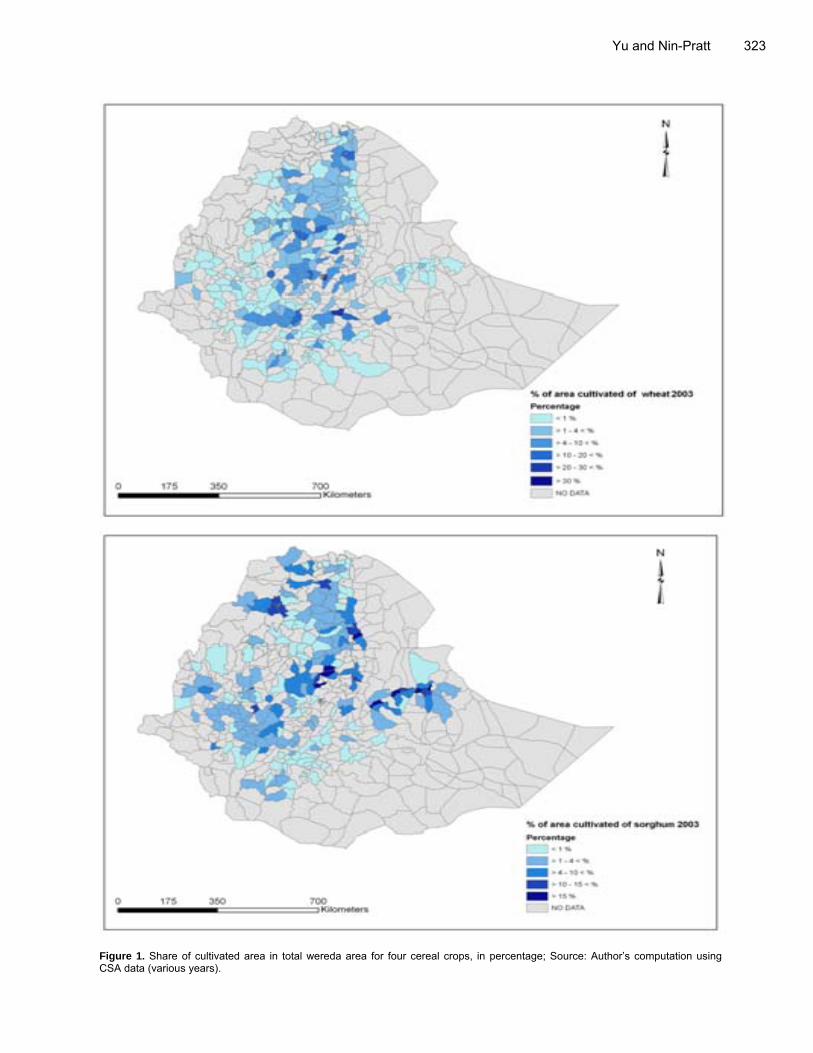
Yu and Nin-Pratt 323
Figure 1. Share of cultivated area in total wereda area for four cereal crops, in percentage; Source: Author’s computation using CSA data (various years).

324 J. Dev. Agric. Econ.

Yu and Nin-Pratt 325
Figure 2. Spatial distribution of fertilizer use in cereal production; Source: Author’s calculation using CSA data (various years).
326 J. Dev. Agric. Econ. whether or not to participate in the fertilizer market. If he/she chooses to participate, the next step is to decide the quantity to purchase. Through this procedure, the DH model allows separation of the sample of farming households into three groups: households adopting fertilizer, households wanting to adopt but reporting no positive application, and households choosing not to adopt. We incorporate this additional information to the DH model to obtain more efficient and consistent estimates of technology adoption. Similar DH model is adopted by Asfaw et al. (2011) to examine the adoption of chickpea seed variety in Ethiopia.
The DH model used in this study has two equations, one explaining access to fertilizer, and the other one explaining the level of application once access to inputs is granted. First, the latent but unobservable variable underlying an individual farmer’s access to
fertilizer can be modeled as:
, (1)
where is a vector of variables that affect access, is the
parameter vector, and e is random variable distributed as normal with mean 0 and variance 1. The unobserved demand for fertilizer
of farmers can be modeled as:
, (2)
where is a vector of variables that determine the demand
function, β is parameter vector, and u is normal random variable
with mean 0 and variance . The observed input demand ( ) is
characterized by the interaction of Equations (1) and (2). A positive use of input like fertilizer is observed only if two thresholds are passed in the decision making process. Hence the farming households are separated into three groups. Group 1 represents the adopters as the farmer has passed the positive demand
threshold ( >0) and has access to input ( > 0). Group 2 in the
sample includes farmers who want input ( >0) but cannot
because of some constraints like lack of access ( ≤ 0). Group 3
consists of farmers who do not want to use input ( < 0) whether
they have access to it or not ( > 0 or ≤ 0).
We assume that the access and demand equations are independent and that the log likelihood function for the sample-separated data can be expressed as:
, (3)
where φ and are the probability density and cumulative
distribution function of the standard normal variable, respectively; 1,
2 and G3 are indicator functions showing whether a given observation belongs to group 1, 2 or 3, respectively. Equation (3) can be estimated using maximum likelihood (ML) techniques, which
gives consistent estimates of the parameters. If and are
independent, the maximum likelihood function can be separated into a probit and a truncated normal regression model. The model specification of the DH estimator can be tested against the Tobit model using a likelihood ratio (LR) test to determine whether the data supports sequential technology adoption decisions or traditional probit and Tobit approaches are sufficient.
We address potential endogeneity of some of the explanatory variables (in particular the variable representing “extension”) using the control function (CF) approach of Rivers and Vuong (1988). According to Imbens and Wooldridge (2008), the CF approach offers some distinct advantages for models that are nonlinear in parameters or endogeneity variables because the CF estimator tackles the endogeneity by adding an additional variable to the regression, generating more precise and efficient estimator than the IV estimator.
After obtaining coefficient estimates for parameters of interest, we can derive the average partial effects (APE) of the explanatory variable across plot and time. The APE is the partial effect averaged across the sample. The first step in obtaining the APE is
to derive the partial effect for the explanatory variable of interest
for each observation in the sample. The partial effect of a variable
on the unconditional expected value of y depends on whether
is an element of access equation (2) or demand equation (1), or
both (Burke, 2009). First, if is an element of both equations, the
partial effect is:
. (4)
If is only determining the probability of Y > 0 in the access
Equation (1), then = 0, and the second term on the right-hand
side of Equation (4) disappears. If is only determining the value
of Y in the demand Equation (2), given that Y > 0, then = 0, and
the first term on the right-hand side is dropped. The APE for a continuous variable is then calculated as the
average of the partial effects. The APE of a binary explanatory variable is calculated as the mean difference between unconditional
expected value, , valued at the binary variable D=0 and D=1.
The APE is generally of greater interest than the partial effect at the average of the sample mean, particularly in nonlinear models and in the case of discrete variables (Imbens and Wooldridge, 2008). However, the APE obtained from the control function approach
outlined above cannot be used for statistical inference. Therefore the bootstrap method is used to obtain the variances of APE and their associated significance levels. Data and descriptive statistics The model in Equation (3) is estimated empirically using data from CSA annual agricultural sample surveys conducted in four years: 2003 to 2004, 2004 to 2005, 2006 to 2007, 2007 to 2008, covering all crop production regions of Ethiopia. More recent years are not included in the analysis because administrative border shifts substantially due to government reconstruction. The surveys are nationally representative under a stratified two-stage cluster sample design. First enumeration areas (EAs) were selected using probability proportional to the number of agricultural households from the census and adjusted for the sub-sampling effect (with the caveat that the survey does not cover the non-sedentary population in some zones). At the second stage, 25 agricultural households, households with at least one member engaged in growing crops and/or raising livestock, from each sample EA were systematically selected at the second stage. Each year more than 2,000 enumeration areas (EAs) were selected, resulting in about 50,000 agricultural households growing cereals and other annual and permanent (perennial) crops. The exact number of EAs and agricultural households covered in the survey varies slightly each year due to cost and other considerations. In the selected rural peasant households the agricultural data were collected from sedentary agricultural holders, who operate the land that is used wholly or partly for agricultural production. Unfortunately due to the nature of the survey, it is impossible to build a panel of households for analysis.
Data on crop production and agricultural practice are recorded at plot level. Information on farming practice of irrigation, using agricultural chemicals, growing a single crop (mono-cropping) and land rental access are binary variables. Extension access is defined as whether the plot under government extension programs. At holder level, variables about access to credit and advisory services are binary variables defined as whether the holder benefit from credit service and agricultural advisory services in the locality. Agricultural advisory service is related with extension but not the same because a holder can have plots not under government extension programs but still receiving advisory service from other organizations like NGOs and vice versa. Land fragmentation is represented by the number of plots operated by the holder, and crop rotation refers to whether the holder practices crop rotation or not. Gender, age, and education grade refer to the holder’s demographic characteristics.
At household level, household size and total cereal area are included to capture household labor and land resources. At community level, having experience with fertilizer is defined as the share of crop area using fertilizer in total cereal area, while the importance of a particular crop is the proportion of the crop area in total cereal area. Knowledge availability in community is captured by the area share of crop land using fertilizer in the wereda (districts in Ethiopia).
Location affects technology adoption through social and agro-
Yu and Nin-Pratt 327 climatic effects, and measures of location and spatially-differentiated variables can explicitly quantify effects of spatial factors on technology uptake and land use. This survey database is complemented by spatial information, incorporating variables that reflect heterogeneity in the quality and availability of natural resources, demographic distribution, and infrastructure and market access.
The spatial variables include market access, population density, road density and land productivity at wereda level. Market access is defined as average travel time in minutes to reach a market of 50,000 or more people (CSA, EDRI and IFPRI, 2007). Road density is the ratio of the length of total road network to land area in the wereda, measured in kilometers per square kilometer (CSA, EDRI and IFPRI, 2007). The road network includes all roads in the country: motorways, highways, main or national roads, and secondary or regional roads. Population density measures the number of persons per square kilometer (CSA, 2010). Crop suitability is calculated based on agro-ecological zones to capture the quality of natural resources for production of the different crops at wereda level. It evaluates land resources and biophysical limitations and potentials for each crop, hence provides the distribution of land, classified into five suitability classes: very suitable, suitable, moderately suitable, marginally suitable and not suitable. Two variables are used to capture suitability for each of the four cereal crops. One variable is area share of highly suitable land, which is the ratio of total very suitable and suitable land in the wereda to total wereda area (EDRI, 2009). The other variable is area share of moderately to marginally suitable land, defined as the ratio of total moderately and marginally suitable land to total wereda area (EDRI, 2009).
Based on Just and Zilberman (1983), we classify explanatory variables for fertilizer access Equation (1) in the DH model and available from CSA data as follows: a) financial constraints -- access to credit; b) fixed costs of adopting the technology; and c) spatial constraints and supply-side effects. Similarly, we group variables affecting the demand of fertilizer (Equation 2) in: a) variables affecting productivity in the use of fertilizer; b) resource availability and risk related variables; and c) spatial variables affecting prices and profitability. Table 3 summarizes the variables used in the analysis.
Variables in the dataset assumed to affect access to inputs (Equation 1) include farmer’s access to extension services, farmers’ characteristics like gender, age and education, and the level of adoption in the district where the farmer is located (measured as the share of the crop using improved technology in total area of that crop in the district). Most of these variables are related to fixed costs incurred when adopting the new technology and result from the farmer’s need to access to knowledge that would allow him/her to implement the new technology We expect a positive relationship between access to fertilizer and access to extension services, education and the level of adoption at the district level. Supply-side effects such as lack of supply, late delivery and inadequate infrastructure are captured by variables representing market access, population and road density and zonal dummies.
Variables explaining demand of fertilizer are irrigation and the use of pesticide and herbicide which we consider respectively as complementary investments and inputs that can increase
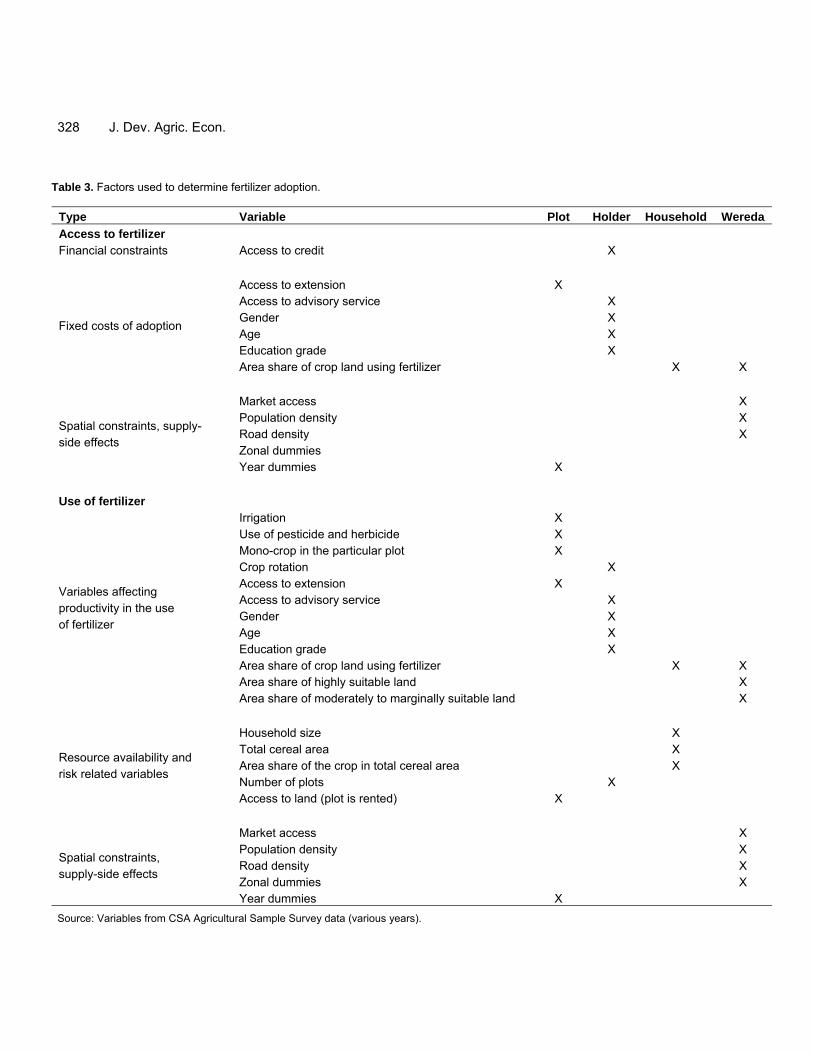
328 J. Dev. Agric. Econ.
Table 3. Factors used to determine fertilizer adoption.
Type Variable Plot Holder Household Wereda
Access to fertilizer Financial constraints Access to credit X
Fixed costs of adoption
Access to extension X Access to advisory service X Gender X Age X Education grade X Area share of crop land using fertilizer X X
Spatial constraints, supply- side effects
Market access X Population density X Road density X Zonal dummies Year dummies X
Use of fertilizer
Variables affecting productivity in the use of fertilizer
Irrigation X Use of pesticide and herbicide X Mono-crop in the particular plot X Crop rotation X Access to extension X Access to advisory service X Gender X Age X Education grade X Area share of crop land using fertilizer X X Area share of highly suitable land X Area share of moderately to marginally suitable land X
Resource availability and risk related variables
Household size X Total cereal area X Area share of the crop in total cereal area X Number of plots X Access to land (plot is rented) X
Spatial constraints, supply-side effects
Market access X Population density X Road density X Zonal dummies X Year dummies X
Source: Variables from CSA Agricultural Sample Survey data (various years).
productivity of fertilizer. Farmer’s characteristics like gender, age and education can also affect demand of fertilizer use. Quality of natural resources measured as suitable area in the district where the farmer is located is used as an indicator of expected crop response to fertilizer. Finally, specialization in a particular crop can facilitate use and improve efficiency in the use of fertilizer. Resource availability and risk related variables are also key determinants in the adoption decision and intensity of fertilizer use. According to Coady (1995), a wealthy farmer usually exhibits decreasing absolute risk aversion but increasing relative risk aversion, meaning that the farmer will tend to use higher absolute levels of inputs but less inputs per hectare than less wealthier producers. We expect variables indicating wealth and capital availability as total area and access to additional land (renting land), to be positively related to fertilizer use, with estimated coefficients smaller than 1 if households are relative risk averse. The share of the crop in total area reflects the importance of the crop in the production system, and we expect this variable to be positively related to fertilizer use. The correlation between household size and fertilizer use should be positive for two reasons. First, we assume that fertilizer application is a labor intensive task, and with the cost of family labor being lower than that of hired labor, a positive coefficient for this variable captures this lower cost of applying fertilizer (Coady, 1995). A second explanation for a positive coefficient of household size is related to risk. With labor being a “safe” asset, compared to crop production, more family labor is equivalent to a higher level of non-stochastic assets, allowing for higher use of fertilizer.
Spatial variables like market access, population density and road density affect the level of fertilizer use through marketing and transportation margins affecting the prices that farmers pay for fertilizer and eventually also the price they receive for their products. Zonal dummies capture other specific spatial effects not captured by other variables. Descriptive statistics Table 4 presents descriptive statistics of explanatory variables in the DH model by group of fertilizer usage for four major cereal crops (barley, maize, teff, and wheat). The table shows substantial differences between technology adopters and non-adopters. Compared to non-adopters, adopters report larger plot size, higher yields, they are more specialized, they show higher use of pesticides and herbicides, they are younger, more educated, more experienced and wealthier than non-adopters (more oxen, crop fields and larger cereal area), and they have better access to extension, credit, advisory services, larger household size. There are also differences in the spatial location of adopters and non-adopters. Adopters tend to have better market access, improved infrastructure (higher road density), they are located in regions with higher population density, better natural endowments (crop suitability), and live in weredas where technology has disseminated broadly. RESULTS AND DISCUSSION Following the framework outlined in the previous section,
Yu and Nin-Pratt 329 the endogeneity of extension is addressed by a control function at plot level. The reduced form equation of endogenous explanatory variable, extension access, is regressed over exogenous variables including land rental, farming practice (mono-crop, chemical use, crop rotation, damage control and irrigation), holder characteristics (gender, age, education grade), access to credit and advisory services, household characteristics (household size, farm size, experience in fertilizer, importance of crop) and wereda fertilizer adoption level. Year dummies are used to control time variations and the error term incorporated cluster effect at EA level. Determinants of fertilizer access Treating extension as endogenous variable, Table 5 reports results of the econometric estimation of the DH model for fertilizer access at plot level. The first result to be noted is that of the Wald test for independent equations at the bottom of the table indicating that the extension service is endogenous in the decision making process of fertilizer adoption. Compared to the coefficients obtained under the assumption of exogenous extension, the coefficients estimated using the CF approach is smaller in the access function, but larger in the demand function. It suggests that extension service boosts the probability of having fertilizer access but does not affect the amount of fertilizer used among users. We also tested the model by checking the hypothesis that farmers make input decisions simultaneously instead of sequentially as assumed by the DH model. To do this we estimated the Tobit and the DH model separately and compared their log-likelihoods (LR test at the bottom of Table 5). We found that the log-likelihood of the DH model is significantly larger than that of the Tobit model, confirming the relative superiority of the DH specification for this dataset over the Tobit model.
Looking at the main results of the model explaining access to chemical fertilizer we find that the main explanation of access to fertilizer is the possibility of reducing the fixed knowledge cost related to adoption of the new technology, mainly through access to extension services. Also important in explaining access to fertilizer is the share of total cereal land under fertilizer both at household level and at the wereda level where the household is located, suggesting that fertilizer is more likely to be adopted in households who have already used this input in other crops, and in districts with better
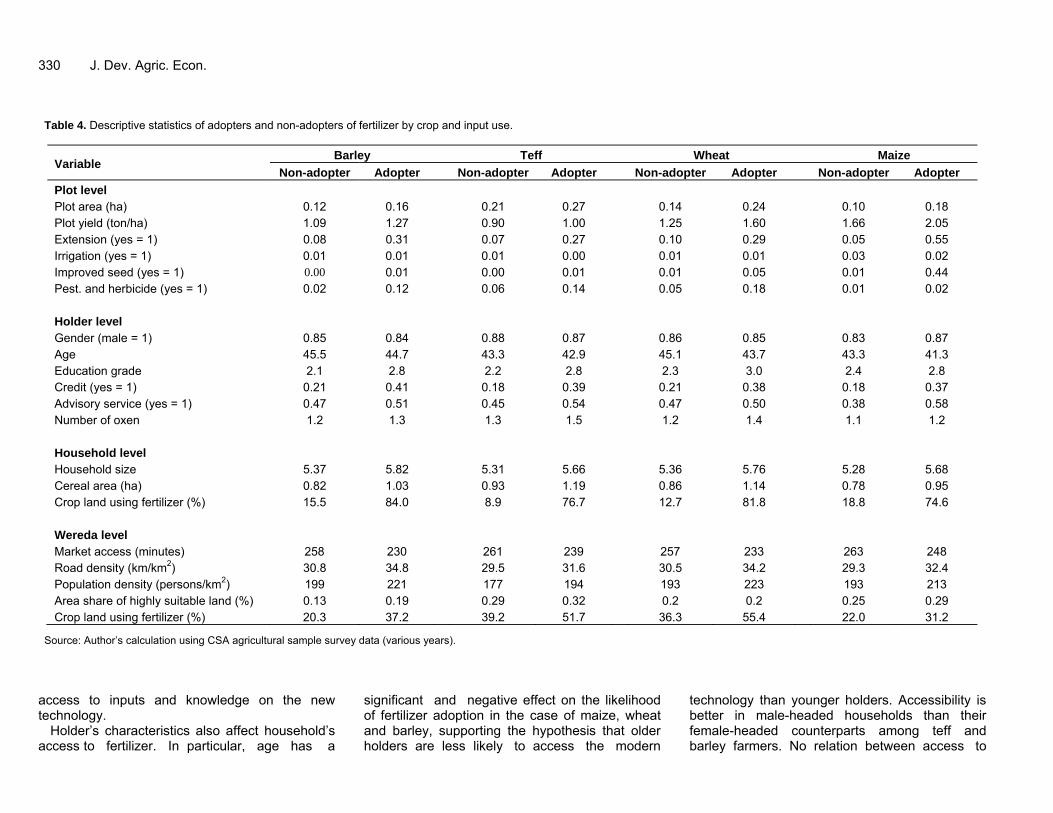
330 J. Dev. Agric. Econ. Table 4. Descriptive statistics of adopters and non-adopters of fertilizer by crop and input use.
Variable Barley Teff Wheat Maize
Non-adopter Adopter Non-adopter Adopter Non-adopter Adopter Non-adopter Adopter
Plot level Plot area (ha) 0.12 0.16 0.21 0.27 0.14 0.24 0.10 0.18 Plot yield (ton/ha) 1.09 1.27 0.90 1.00 1.25 1.60 1.66 2.05 Extension (yes = 1) 0.08 0.31 0.07 0.27 0.10 0.29 0.05 0.55 Irrigation (yes = 1) 0.01 0.01 0.01 0.00 0.01 0.01 0.03 0.02 Improved seed (yes = 1) 0.00 0.01 0.00 0.01 0.01 0.05 0.01 0.44 Pest. and herbicide (yes = 1) 0.02 0.12 0.06 0.14 0.05 0.18 0.01 0.02
Holder level
Gender (male = 1) 0.85 0.84 0.88 0.87 0.86 0.85 0.83 0.87 Age 45.5 44.7 43.3 42.9 45.1 43.7 43.3 41.3 Education grade 2.1 2.8 2.2 2.8 2.3 3.0 2.4 2.8 Credit (yes = 1) 0.21 0.41 0.18 0.39 0.21 0.38 0.18 0.37 Advisory service (yes = 1) 0.47 0.51 0.45 0.54 0.47 0.50 0.38 0.58 Number of oxen 1.2 1.3 1.3 1.5 1.2 1.4 1.1 1.2
Household level Household size 5.37 5.82 5.31 5.66 5.36 5.76 5.28 5.68 Cereal area (ha) 0.82 1.03 0.93 1.19 0.86 1.14 0.78 0.95 Crop land using fertilizer (%) 15.5 84.0 8.9 76.7 12.7 81.8 18.8 74.6
Wereda level
Market access (minutes) 258 230 261 239 257 233 263 248 Road density (km/km2) 30.8 34.8 29.5 31.6 30.5 34.2 29.3 32.4 Population density (persons/km2) 199 221 177 194 193 223 193 213 Area share of highly suitable land (%) 0.13 0.19 0.29 0.32 0.2 0.2 0.25 0.29 Crop land using fertilizer (%) 20.3 37.2 39.2 51.7 36.3 55.4 22.0 31.2
Source: Author’s calculation using CSA agricultural sample survey data (various years). access to inputs and knowledge on the new technology.
Holder’s characteristics also affect household’s access to fertilizer. In particular, age has a
significant and negative effect on the likelihood of fertilizer adoption in the case of maize, wheat and barley, supporting the hypothesis that older holders are less likely to access the modern
technology than younger holders. Accessibility is better in male-headed households than their female-headed counterparts among teff and barley farmers. No relation between access to

Yu and Nin-Pratt 331
Table 5. Double hurdle regression estimates for fertilizer access.a
Variable Maize Teff Wheat Barley
Coefficient P > z Coefficient P > z Coefficient P > z Coefficient P > z
Fertilizer access (yes=1)
Credit (yes = 1) -0.094 0.000 0.027 0.185 0.067 0.002 -0.115 0.000
Extension (yes = 1) 2.646 0.000 0.014 0.902 0.231 0.059 1.611 0.000
Advisory service (yes = 1) -0.299 0.000 0.012 0.677 0.070 0.083 -0.263 0.000 Gender (male = 1) 0.013 0.527 0.093 0.000 -0.000 0.987 0.067 0.024 Age -0.002 0.000 0.001 0.306 -0.003 0.000 -0.004 0.000 Education grade 0.004 0.173 -0.003 0.440 0.001 0.828 0.000 0.997 Area share of total crop land using fertilizer (household) 0.022 0.000 0.040 0.000 0.035 0.000 0.031 0.000 Area share of total crop land using fertilizer (wereda) 0.010 0.000 0.012 0.000 0.013 0.000 0.013 0.000 Market access (wereda) -0.000 0.000 0.000 0.001 -0.001 0.000 -0.000 0.000 Population density (wereda) 0.000 0.048 -0.000 0.037 0.000 0.162 -0.000 0.854 Road density (wereda) -0.001 0.000 -0.001 0.000 -0.001 0.001 -0.001 0.007 Generalized residual -0.477 0.000 0.497 0.000 0.383 0.000 -0.449 0.000 Constant -2.652 0.000 -2.450 0.000 -2.322 0.001 -3.827 0.000 Observations 110162 89533 60228 62026 Log likelihood -167.6 4820 7412 3635 P-value of Wald test of indep. eqns. (rho = 0) 0.274 0.000 0.290 0.000 0.257 0.000 0.259 0.000 P-value of LR test of Tobit model 19983 0.000 25783 0.000 21405 0.000 12830 0.000
Note: a Extension is treated as an endogenous variable; Source: Author’s calculation using CSA data (various years). fertilizer and education was found.
The spatial variables included to explain access do not appear to have major impact as their coefficients are quite small. In the case of maize, the spatial effects are better captured by the zonal dummies (not reported). Access to fertilizer in maize production is more likely in the south and southwest, around Awasa and Jimma, in West Oromia, and in the zones crossed by the major road going east to Djibouti: West and East Hararge, West Arsi and Harari). Coefficients of the dummy variables in the case of teff show that
farmers of some zones in SNNP and in particular in Amhara with high teff production have difficulties to access the technology. In the case of wheat, none of the coefficients of the zonal dummy variables is significant, indicating that only variables related to fix costs of the technology are relevant explaining access to fertilizer. Determinants of fertilizer demand Results for the estimation of the model explaining
area planted using fertilizer conditional on access to fertilizer at plot level are presented in Table 6. The conditional area under fertilizer is mainly explained by: specialization in the particular crop (mono crop production at the plot level); access to inputs through extension specialist; previous knowledge and experience in cereal production (crop rotation); access to land rental market and land fragmentation; total cereal area; share of the crop in total household cultivated cereal area; and the area under fertilizer in the wereda.
The area under cereal production is positively

332 J. Dev. Agric. Econ.
Table 6. Double hurdle regression estimates for fertilizer use.
Variable Maize Teff Wheat Barley
Coefficient P>z Coefficient P>z Coefficient P>z Coefficient P>z
Area under chemical fertilizer Irrigation (yes = 1) -0.049 0.216 -0.208 0.000 -0.136 0.003 -0.044 0.561 Pesticides and herbicides (yes = 1) 0.019 0.547 0.053 0.000 0.055 0.000 0.089 0.000 Mono-crop (yes = 1) 0.243 0.000 0.132 0.000 0.514 0.000 0.157 0.000 Crop rotation (yes = 1) 0.039 0.008 0.034 0.004 0.055 0.000 0.006 0.769 Extension (yes = 1) 0.187 0.005 0.102 0.005 0.071 0.097 0.148 0.017 Advisory service (yes = 1) -0.015 0.505 -0.024 0.037 -0.014 0.363 -0.026 0.237 Gender (male = 1) 0.076 0.000 0.029 0.000 0.020 0.014 0.020 0.182 Age 0.001 0.000 0.003 0.000 0.003 0.000 0.002 0.000 Education grade -0.007 0.000 0.001 0.114 -0.000 0.813 0.004 0.046 Area share of total crop land using fertilizer 0.000 0.525 0.000 0.045 -0.000 0.135 -0.000 0.142 Area share of total crop land using fertilizer (wereda) 0.001 0.043 -0.001 0.000 0.001 0.007 0.002 0.000 Share of highly suitable land 0.025 0.160 0.005 0.785 0.018 0.378 -0.062 0.019 Share of moderately to marginally suitable land -0.018 0.542 -7.185 0.024 0.573 0.000 -0.098 0.082 Household size 0.000 0.783 -0.001 0.217 0.004 0.002 0.002 0.347 Cereal area of household 0.317 0.000 0.182 0.000 0.155 0.000 0.281 0.000 Share of the crop in total cereal area 0.006 0.000 0.004 0.000 0.004 0.000 0.007 0.000 Number of plots under holder -0.047 0.000 -0.044 0.000 -0.038 0.000 -0.057 0.000 Plot is rent (yes = 1) 0.050 0.001 0.000 0.992 0.038 0.000 0.105 0.000 Market access 0.000 0.000 0.000 0.000 0.000 0.411 0.000 0.449 Population density -0.000 0.000 -0.000 0.017 -0.000 0.001 -0.000 0.160 Road density 0.000 0.478 -0.000 0.000 -0.001 0.000 -0.001 0.000 Generalized residual -0.041 0.290 -0.054 0.011 -0.020 0.419 -0.076 0.026 Constant -0.676 0.000 -0.420 0.000 -0.443 0.551 -1.626 0.005 Log-likelihood -10040.9 71.4 -30098 -16162
Note: a Extension is treated as an endogenous variable; Source: Author’s calculation using CSA data (various years). associated with area using fertilizer. The coefficients of advisory services are far smaller and can be insignificant, suggesting extension is
the dominants source of knowledge for holders. In addition, farmers increase fertilizer application of a particular cereal crop if the crop is important in the
production system (captured by the crop’s area share). Households that rent land for crop production tend to have larger area under fertilizer

than those without access to land. Similar to total land under cereal production, having access to land rental market results in an increase in the area using fertilizer but a reduced share of fertilized area in total cereal land. Coefficients obtained for land rental in different crops support the hypothesis that households compensate forthe additional risk of increasing area of a crop by reducing input intensity for that crop.
In contrast with other studies (e.g. Croppenstedt et al., 2003), family size does not play a significant role determining fertilizer use. As fertilizer is assumed to be a labor intensive technology, it is expected that availability of family labor would result in higher fertilizer use. Only in the case of wheat we find that household size is positively and significantly related to area under fertilizer. A possible explanation for our results is that farmers make their decisions of the area applied fertilizer mainly based on the crop growing in the plot, and the availability of labor is not a constraint yet given the relatively low adoption rate of fertilizer.
Among holder characteristics we find that age has a positive and statistically significant effect on fertilizer demand in all crops suggesting that among adopters, farming experience is related to efficiency and adoption in the use of fertilizer, at both household and wereda level. We also find a significant effect of gender in conditioning fertilizer demand and households with more educated head exhibit higher fertilizer adoption in barley production but not in the case maize. With the exception of market access for maize and teff, the coefficients of spatial variables (crop suitability, population and road density) are negligible, indicating that biophysical and demographic conditions are not the major constraints in fertilizer adoption in Ethiopia. Average partial effects As identification and estimation of average effects become more complicated in the case of nonlinear models with discrete variables, as in this study, it is not easy to examine and compare the effect on fertilizer adoption from different influencing factors. The average partial effect (APE) is hence introduced to measure the average change in technology adoption due to a change in the variables of interest. We obtained average partial effects by bootstrapping the estimated model and results after 500 iterations are reported in Table 7. These results show that extension has a significant positive effect on
Yu and Nin-Pratt 333 fertilizer adoption. For example, households having access to extension can increase the average maize area under fertilizer by 0.1 ha.
The higher the share of crop area under fertilizer at household and district level the higher fertilizer use. Farmers’ own skills and knowledge, represented by mono crop, crop rotation, and uses of chemicals, all contribute to the quantity of fertilizer used. APEs of variables associated with household wealth confirm that households have exhibited decreasing absolute risk aversion but increasing relative risk aversion. Fragmented land plots prevent wide adoption of technology, while on average a plot managed by a male holder tends to show higher fertilizer use, than those managed by younger female holders. APE results also suggest that although infrastructure related factors like market access, and population and road density do have an impact on fertilizer adoption, their effects are small and not comparable with the agroecological constraints defined by crop suitability.
Ranked by APE, the top three factors affecting average change in area using fertilizer are extension, mono-crop and total area for cereal production. Similarly, Extension, cereal area and mono-crop are found major contributors in changes in fertilizer adoption. Our results are consistent with previous studies on fertilizer adoption in Ethiopia, especially in the role of extension and farmers’ experience. Conclusion Extension services have played a central role in facilitating access to the promoted technology, as it is the instrument to disseminate new technology package including seed, fertilizer and new farming practice. Ethiopia’s agricultural extension system is one of the largest in the world, with over 60,000 development agents working in nearly 10,000 farmer training centers throughout the country. This paper aims to understand the extent and determinants of fertilizer adoption in the country. A double hurdle model is chosen, which allows us to analyze separately the factors affecting access of farmers to the new technology and demand for fertilizer conditional to access in a sequential approach, addressing the endogeneity of extension service. Built on the framework of Asfaw et al. (2011), the study is the first to estimate fertilizer adoption using nationally representative data from Ethiopia Agricultural Sample

334 J. Dev. Agric. Econ. Table 7. Average partial effects of factors on chemical fertilizer adoption.
Average increase in area under fertilizer (ha) Maize Teff Wheat Barley
APE t-value APE t-value APE t-value APE t-value
Variables in both demand and access equations Extension (yes = 1) 0.1007 7.9 0.0209 2.6 0.0184 2.2 0.0342 5.4 Advisory service (yes = 1) -0.0056 -4.0 -0.0043 -2.0 -0.0012 -0.4 -0.0046 -3.7 Gender (male = 1) 0.0040 5.5 0.0072 4.7 0.0034 0.9 0.0017 1.9 Age 0.0000 0.9 0.0005 8.4 0.0004 6.9 0.0001 3.3 Education grade -0.0003 -3.2 0.0002 0.9 -0.0001 -0.2 0.0002 1.6 Area share of total crop land using fertilizer (household) 0.0004 22.6 0.0010 36.4 0.0007 22.5 0.0004 22.1 Area share of total crop land using fertilizer (wereda) 0.0002 11.8 0.0001 4.9 0.0003 10.7 0.0003 16.4 Market access 0.0000 1.1 0.0000 10.8 0.0000 -1.1 0.0000 -1.2 Population density 0.0000 -2.2 0.0000 -3.0 0.0000 -0.4 0.0000 -1.0 Road density 0.0000 -0.7 -0.0001 -5.6 -0.0002 -3.8 -0.0001 -5.7 Variables in demand equation only Irrigation (yes = 1) -0.0024 -1.1 -0.0319 -5.9 -0.0212 -3.4 -0.0019 -0.6 Pesticides & herbicides (yes = 1) 0.0010 0.5 0.0099 6.1 0.0092 5.8 0.0043 5.3 Mono-crop (yes = 1) 0.0135 12.6 0.0243 3.5 0.0928 9.7 0.0074 4.0 Crop rotation (yes = 1) 0.0020 1.8 0.0060 2.2 0.0085 2.4 0.0003 0.3 Share of highly suitable land 0.0013 1.3 0.0009 0.3 0.0035 0.9 -0.0028 -2.1 Share of moderately to marginally suitable land -0.0009 -0.5 -1.3125 -2.5 0.0876 4.4 -0.0045 -1.6 Household size 0.0000 0.2 -0.0002 -1.1 0.0006 1.5 0.0001 0.8 Cereal area of household 0.0166 18.4 0.0332 33.5 0.0267 30.8 0.0129 24.1 Share of the crop in total cereal area 0.0003 29.7 0.0008 34.5 0.0008 31.8 0.0003 28.1 Number of plots under holder -0.0025 -16.7 -0.0081 -18.7 -0.0065 -25.1 -0.0026 -19.4 Plot is rent (yes = 1) 0.0027 3.1 0.0000 0.0 0.0067 4.6 0.0052 6.1
Source: Author’s calculation using CSA data (various years).
Surveys while considering model endogeneity using a control function approach.
The major findings are presented below, centered on the impact of extension. First, statistical tests allow us to examine several theoretical and methodological assumptions laid out at the start of the study. The studyconfirms the endogeneity of extension service in the decision
making process of fertilizer adoption. Log-likelihood test also indicates that farmers make input decisions sequentially, not simultaneously, highlighting the relative superiority of the DH specification for this analysis. Average partial effect from bootstrapping process is appropriate in inspecting the unconditional effects of factors that influence the adoption process because it is
especially helpful in cases when there are observations with zero values for input use.
Second, extension service boosts fertilizer use, which corroborates with many other studies on fertilizer adoption in Ethiopia (Beshir et al., 2012; Carlsson et al., 2005; Wubeneh and Sanders, 2006; Noltze et al., 2012). Extension not only increases the probability of adoption fertilizer but

Yu and Nin-Pratt 335
Figure 3. Yield distributions of cereals at the plot level different input combinations (average values 2003-2007 in kilograms per hectare); Source: Author’s computation using CSA agricultural sample survey data.
expand the area planted using fertilizer conditional on access to fertilizer. Farmers face a high “knowledge” cost related to adoption of new technology and extension services helps cut the adoption cost (Asfaw and Admassie, 2004). Education and past experience can also effectively lower the adoption barrier and hence promote the diffusion of new technology, which were also identified in earlier studies by Admassie and Ayele (2004) and Beshir et al. (2012). Other factors affects fertilizer use includes household wealth, access to land rental market, land fragmentation and the importance of the crop in the production system.
Third, similar to Dercon and Christiaensen (2011), risk aversion behavior can have a considerable impact on farmer’s fertilizer adoption decision. Having access to land rental market can increase the area using fertilizer but reduce the share of fertilized area in total cereal land, suggesting that households compensate for the additional risk of increasing area of a crop by reducing input intensity for that crop. In addition, variables associated with household wealth confirm that households have exhibited decreasing absolute risk aversion but increasing relative risk aversion.
Fourth, spatial variables obtained through GIS tools are introduced in the analysis to capture of biophysical constraints and infrastructure factors like crop suitability and market access. Although we find market access and road density do have an impact on fertilizer adoption, their effects are small and not comparable with the agroecological constraints defined by crop suitability and other local agronomic and development conditions (Diao and Nin-Pratt, 2005; Tadesse et al., 2006). Substantial yield gain in maize and teff can be achieved if technology is provided through a locally tailored extension package. This translates into the need of an extension package focusing on improving access to technological packages that are adapted to local agroecological conditions to fully realize the potential.
Although the results of this analysis highlight the important role and great potential of extension in the development of Ethiopia agriculture, the impacts of the strategy to raise cereal production and yields through extension have been mixed, as fertilizer use increased but access to extension and productivity growth remain low among farmers in the country. Some potential constraints could compromise the effectiveness of the

336 J. Dev. Agric. Econ. extension system, including service mismatching farmers’ need, deficiency of resources, low capabilities and knowledge of extension workers and lack of transparency and motivations. Readers can refer to Davis et al. (2010) for detailed discussion on these constraints.
One problem observed from the data and that it is not necessarily captured by the DH model is the great yield variability among producers using fertilizers (Figure 3). First, the median of the yield distribution obtained using fertilizer + seed in maize and wheat is larger than that of the traditional technology but far from the expectations that the authorities had of doubling yields when the program was launched. Second, the highest yields (the 90th percentile of the distribution) are close to those obtained in trials and experiments during the first face of PADETES (3,700 kg/ha in maize and close to 3,000 kilograms per hectare in wheat). Reducing the high variability observed in yields with fertilizer+seed technology should result in movements of the mean and median of the yield distribution closer to what today are “frontier” values (high yield) resulting in improved conditions and incentives to adopt the technology. Third, median yields obtained in teff and barley using fertilizer technology are low and similar to those obtained using the traditional technology, with frontier values in the improved technology being much lower than those obtained with the traditional technology. This suggests that availability of improved varieties in teff and barley is still a major constrain to increase yields and that the only technical alternative to the traditional technology is the use of chemical fertilizer. The possibilities of increasing yields of these crops using fertilizer only are quite limited. Conflict of Interests The author(s) have not declared any conflict of interests. ACKNOWLEDGEMENTS The authors acknowledge the significant contribution of José Funes and Sinafikeh Asrat Gemessa to an early version of this paper. REFERENCES Abebaw D, Haile MG (2013). The impact of cooperatives on agricultural
technology adoption: Empirical evidence from Ethiopia. Food Policy 38:82–91. http://dx.doi.org/10.1016/j.foodpol.2012.10.003
Admassie A, Ayele G (2004). Adoption of improved technology in
Ethiopia. Addis Ababa, Ethiopia: Ethiopia Development Research Institute. PMid:16895031
Asfaw A, Shiferaw B, Simtowe F, Haile MG (2004). Agricultural technology adoption, seed access constraints and commercialization in Ethiopia. J. Dev. Agric. Econ. 3(9):436-447.
Beshir H, Emana B, Kassa B, Haji J (2012). Determinants of chemical fertilizer technology adoption in North eastern highlands of Ethiopia: the double hurdle approach. J. Res. Econ. Int. Finan. 1(2):39-49.
Burke WJ (2009). Fitting and interpreting Cragg's tobit alternative using Stata. The Stata J. 9(4):584-592.
Byerlee D, Spielman DJ, Alemu D, Gautam M (2007). Policies to promote cereal intensification in Ethiopia: A review of evidence and experience. Discussion Paper 00707. Washington, DC: International Food Policy Research Institute.
Carlsson F, Kohlin G, Mekonnen A, Yesuf M (2005). Are agricultural extension packages what Ethiopian farmers want? A stated preference analysis. Working Papers in Economics. Department of Economics, Goteborg University. P. 172.
Coady DP (1995). An empirical analysis of fertilizer use in Pakistan. Economica 62:213–234. http://dx.doi.org/10.2307/2554904
Cragg JG (1971). Some statistical models for limited dependent variables with applications to the demand for durable goods. Econometrica 39:829–844. http://dx.doi.org/10.2307/1909582
Croppenstedt A, Demeke M, Meschi M (2003). Technology adoption in the presence of constraints: The case of fertilizer demand in Ethiopia. Rev. Dev. Econ. 7(1):58-70. http://dx.doi.org/10.1111/1467-9361.00175
CSA. Various years. Annual agricultural sample survey (database). Central Statistical Agency. Last accessed September 2011, http://www.csa.gov.et/
CSA, EDRI and IFPRI. 2007. Atlas of Ethiopia Population and Housing Census. Central Statistical Agency, Ethiopian Development Research Institute, and International Food Policy Research Institute, Addis Ababa, Ethiopia.
Davis K, Swanson B, Amudavi D, Mekonnen DA, Flohrs A, Riese J, Lamb C, Zerfu E (2010). In-depth assessment of the public agricultural extension system of Ethiopia and recommendations for improvement. Discussion Paper 01041. Washington, DC: International Food Policy Research Institute.
Dercon S, Christiaensen L (2011). Consumption risk, technology adoption and poverty traps: Evidence from Ethiopia. J. Dev. Econ. 96(2):159-173. http://dx.doi.org/10.1016/j.jdeveco.2010.08.003
Diao X, Nin -Pratt A (2005). Growth options and poverty reduction in Ethiopia: A spatial, economy-wide model analysis for 2004-15. DSGD Discussion, Washington, DC: International Food Policy Research Institute. P. 20.
EDRI (2009). Crop suitability analysis– agroecological zones. Addis Ababa, Ethiopia: Ethiopian Development Research Institute.
Holden ST, Shiferaw B, Pender J (2001). Market imperfections and land productivity in the Ethiopian highland. J. Agric. Econ. 52(3):53–70. http://dx.doi.org/10.1111/j.1477-9552.2001.tb00938.x
Howard J, Crawford E, Kelly V, Demeke M, Jeje JJ (2003). Promoting high-input maize technologies in Africa: The Sasakawa-Global 2000 experience in Ethiopia and Mozambique. Food Policy 28:335–348. http://dx.doi.org/10.1016/j.foodpol.2003.08.008
Imbens G, Wooldridge JM (2008). Control function and related methods. Applied Microeconometrics Workshop Lecture Notes.
Just RE, Zilberman D (1983). Stochastic structure, farm size, and technology adoption in developing agriculture. Oxford Econ. 35(2):307–328.

Liverpool-Tasie LSO, Winter-Nelson A (2009). Poverty Status and the
Impact of Formal Credit on Technology Use and Wellbeing among Ethiopian Smallholders. World Dev. 38(4):541–554. http://dx.doi.org/10.1016/j.worlddev.2009.11.006
Liverpool-Tasie LSO, Winter-Nelson A (2012). Social Learning and Farm Technology in Ethiopia: Impacts by Technology, Network Type, and Poverty Status. J. Dev. Stud. 48(10):1505–1521. http://dx.doi.org/10.1080/00220388.2012.693167
Noltze M, Schwarze S, Qaim M (2012). Understanding the adoption of system technologies in smallholder agriculture: The system of rice intensification (SRI) in Timor Leste. Agric. Syst. 108:64-73. http://dx.doi.org/10.1016/j.agsy.2012.01.003
Pender J, Kerr JM (1998). Determinants of farmers' indigenous soil and water conservation investments in semi-arid India. Agri. Econ. 19:113–125.http://dx.doi.org/10.1016/S0169-5150(98)00026-7
Rivers D, Vuong QH (1988). Limited information estimators and exogeneity tests for simultaneous probit models. J. Econometr. 39:347-366. http://dx.doi.org/10.1016/0304-4076(88)90063-2
Yu and Nin-Pratt 337 Shiferaw BA, Kebede TA, You L (2008). Technology adoption under
seed access constraints and the economic impacts of improved pigeonpea varieties in Tanzania. Agric. Econ. 39:309-323.
Tadesse M, Alemu B, Bekele G, Tebikew T, Chamberlin J, Benson T (2006). Atlas of the Ethiopian Rural Economy. Addis Ababa, Ethiopia: Ethiopian Development Research Institute.
Wubeneh NG, Sanders JH (2006). Farm-level adoption of sorghum technologies in Tigray, Ethiopia. Agri. Systems 91:122-134. http://dx.doi.org/10.1016/j.agsy.2006.02.002
World Bank (2006). Ethiopia: Policies for pro-poor agricultural growth. Washington, DC.

Journal of Development and Agricultural
Economics
Related Journals Published by Academic Journals
■ Journal of Plant Breeding and Crop Science■ African Journal of Agricultural Research■ Journal of Horticulture and Forestry■ International Journal of Livestock Production■ International Journal of Fisheries and Aquaculture■ Journal of Cereals and Oilseeds■ Journal of Soil Science and Environmental Management■ Journal of Stored Products and Postharvest Research