journal of educational and behavioral ... - moodle.eduhk.hk

http://jebs.aera.netBehavioral Statistics

Journal of Educational and

http://jeb.sagepub.com/content/35/3/336The online version of this article can be found at:

DOI: 10.3102/1076998609353111

2010 35: 336JOURNAL OF EDUCATIONAL AND BEHAVIORAL STATISTICSSun-Joo Cho and Allan S. Cohen

A Multilevel Mixture IRT Model With an Application to DIF

Published on behalf of

American Educational Research Association

and

http://www.sagepublications.com

found at: can beJournal of Educational and Behavioral StatisticsAdditional services and information for

http://jebs.aera.net/alertsEmail Alerts:

http://jebs.aera.net/subscriptionsSubscriptions:

http://www.aera.net/reprintsReprints:

http://www.aera.net/permissionsPermissions:

What is This?

- Aug 13, 2010Version of Record >>

at HONG KONG INST OF EDUCATION on November 23, 2011http://jebs.aera.netDownloaded from

http://jebs.aera.net

http://jeb.sagepub.com/content/35/3/336

http://www.aera.net

http://www.sagepublications.com

http://jebs.aera.net/alerts

http://jebs.aera.net/subscriptions

http://www.aera.net/reprints

http://www.aera.net/permissions

http://jeb.sagepub.com/content/35/3/336.full.pdf

http://online.sagepub.com/site/sphelp/vorhelp.xhtml


A Multilevel Mixture IRT Model With an Application

to DIF

Sun-Joo Cho

Vanderbilt University

Allan S. Cohen

University of Georgia

Mixture item response theory models have been suggested as a potentially

useful methodology for identifying latent groups formed along secondary,

possibly nuisance dimensions. In this article, we describe a multilevel mixture

item response theory (IRT) model (MMixIRTM) that allows for the possibility

that this nuisance dimensionality may function differently at different levels.

A MMixIRT model is described that enables simultaneous detection of

differences in latent class composition at both examinee and school levels.

The MMixIRTM can be viewed as a combination of an IRT model, an

unrestricted latent class model, and a multilevel model. A Bayesian

estimation of the MMixIRTM is described including analysis of label

switching, use of priors, and model selection strategies. Results of a

simulation study indicated that the generated parameters were recovered very

well for the conditions considered. Use of MMixIRTM also was illustrated

with the standardized mathematics test.

Keywords: finite mixture modeling; item response theory; multilevel modeling; MCMC

Introduction

Mixture item response theory (MixIRT) models have been studied for use in

describing a number of important effects in test data including differential use of

response strategies (Bolt, Cohen, & Wollack, 2001; Mislevy & Verhelst, 1990;

Rost, 1990), speededness (Bolt, Cohen, & Wollack, 2002; Yamamoto &

The research for this study was funded by the 2006-2007 College Board Research Grant Program.

The authors would like to especially thank Dr. Wayne Camara and Dr. Vytas Laitusis for their

support. We also thank an anonymous reviewer and the editor for their insightful comments and

suggestions. The authors also thank Dr. Paul De Boeck and Dr. Sophia Rabe-Hesketh for their

valuable comments. Any opinions, findings, or conclusions are those of the authors and do not

necessarily reflect the views of the supporting agency.

Journal of Educational and Behavioral Statistics

June 2010, Vol. 35, No. 3, pp. 336–370

DOI: 10.3102/1076998609353111

# 2010 AERA. http://jebs.aera.net

336



Everson, 1997), the impact of testing accommodations (Cohen, Gregg, & Deng,

2005), and detection of differential item functioning (DIF; Cohen & Bolt, 2005;

Samuelsen, 2005). The utility of MixIRT models is that they provide a means of

detecting groups formed by dimensionality arising directly from the test data. To

the extent these groups are substantively meaningful, they provide a potentially

important means of understanding how and why examinees respond the way

they do.

In this regard, Rost (1990, 1997) described a mixture Rasch model (MRM) in

which an examinee population is assumed to be composed of a fixed number of

discrete latent classes. In each latent class, a Rasch model is assumed to hold, but

each class may have different item difficulty parameters. The probability of a

correct response in the MRM can be given as

P yijg ¼ 1jg; yjg

� �¼ 1

1þ exp � yjg � big

� �� ; ð1Þ

where g ¼ 1; . . . ;G is an index for latent class, j ¼ 1; . . . ; J is an index for exam-

inees, yjg is the latent ability of examinee j within class g, and big is the Rasch

difficulty parameter of item i for class g. The structure of ability in the MRM is

yjg � N mg;s2g

� �; ð2Þ

where mg is a class-specific mean of ability and s2g is a class-specific variance of

ability.

Rost (1990) suggested that the primary diagnostic potential of the MRM is in

its use in accounting for qualitative differences among examinees and simultane-

ously to quantify ability with respect to the same items. The MRM is used to

identify latent classes of examinees that are homogeneous with respect to item

response patterns. The members of each latent class vary in ability, and the

response strategies differ among classes. Based on this rationale, in this study,

we use an MRM to investigate DIF among latent classes. An important limitation

of MRM is that it essentially ignores the basic multilevel structure that is present

beyond the student level in much of educational test data.

Multilevel models, also known as hierarchical linear models (HLM), allow the

natural multilevel structure of educational and psychological data to be repre-

sented formally in the analysis (Bryk & Raudenbush, 1992; Goldstein, 1987;

Longford, 1993). The combination of HLM with IRT is advantageous, as it pro-

vides more accurate estimates of the standard errors of the model parameters

(Fox, 2005; Maier, 2001, 2002). This combination has led to the development

of psychometric models for item response data that contain hierarchical struc-

ture, thus enabling a researcher to study the impact of different predictors such

as schools and curriculum on the lower level units such as students (e.g., Fox

& Glas, 2001; Kamata, 2001; Maier, 2001, 2002; Rabe-Hesketh, Skrondal, &

Pickles, 2004). A limitation of multilevel IRT models, from the perspective of

A Multilevel Mixture IRT Model

337



mixture IRT modeling, is that they do not provide information about group mem-

bership beyond that given by manifest predictors included in the model.

In this study, we incorporate that multilevel structure into a mixture IRT

model and extend the model into a multilevel mixture IRT model (MMixIRTM).

This MMixIRTM is then used to detect and compare latent groups in the data that

have different measurement characteristics. The utility of this approach lies in the

fact that latent groups, although not immediately observable, are defined by

certain shared response propensities that can be used to help explain item level

performance about how members of one latent group differ from another. It is

these differences in response propensities that help explain the potential causes

of these differential measurement characteristics. The approach proposed in this

study provides this information at the student and school levels along with infor-

mation describing the composition of the different latent groups. We begin below

by illustrating how the MMixIRTM can be viewed as incorporating features from

multilevel models to form a general MMixIRTM.

Multilevel Mixture IRT Model

The proposed MMixIRTM has mixtures of latent classes at two levels, a stu-

dent level and a school level. Student-level latent classes capture the association

between the responses at the student-level unit. The MixIRT model assumes that

there may be heterogeneity in response patterns at the student level, which should

not be ignored (Mislevy & Verhelst, 1990; Rost, 1990). The MMixIRTM does

not exclude the possibility, however, that there may be no student-level latent

classes. It is interesting to note that, if no student-level latent classes exist, this

would indicate that there would also be no school-level latent classes. The reason

is that school-level units are clustered based on the likelihood of their students

belonging to one of the latent classes. In a MMixIRTM as presented in this study,

in other words, it is not meaningful to have school-level classes if no student-

level latent classes are present.

Viewed in this way, school-level latent classes capture the association

between the students within school-level units (Vermunt, 2003). Latent classes

at the school level, however, may differ in the probability that students belong

to particular latent classes. This is accommodated in the MMixIRTM by allowing

for the possibility that school-level latent classes may differ in the proportions of

students in each student-level latent class contained in a school-level latent class.

The probability of getting a correct response in the MMixIRTM can be given

as follows:

P yijt ¼ 1jg; k; yjtgk

� �¼ 1

1þ exp � yjtgk � bigk

� �� ; ð3Þ

where g ¼ 1; . . . ;G is an index for student-level latent classes, k ¼ 1; . . . ;K is

an index for school-level latent classes, j ¼ 1; . . . ; J is an index for examinees,

Cho and Cohen

338



t ¼ 1; . . . ; T is an index for schools, for a test of i ¼ 1; . . . ; I items, yjtgk is the

ability of examinee j in school t and in latent classes g and k, and bigk is the dif-

ficulty of item i for latent classes g and k.

Mixture Proportion Structure of MMixIRTM

There are two mixture proportions in MMixIRTM, pgjk and pk . The pgjk indi-

cate the relative sizes of latent classes at the student-level conditional on latent

class membership at the school level, and pk is the proportion of schools for each

class. As shown in Table 1, there are K probability arrays, p1:Gjk , k ¼ 1; . . . ;K,

where G is the dimension of each array.

Item Difficulty Structure of MMixIRTM

In the general MMixIRTM, item difficulty parameters have both student- and

school-level class-specific values. These can be represented as bigk , which is an

interaction effect of the student-level latent class (g) and school-level latent class

(k). The meaning of an interaction effect is that the characteristics of school-level

latent classes change as the number of school-level DIF items increases.

Ability Structure

As indicated in Equation 4, abilities yjtgk have mean mgk and variance s2gk as

follows:

yjtgk � N mgk ;s2gk

� �: ð4Þ

yjtgk is reparameterized into s2gk � Zjtgk where Zjtgk � Normalðmgk ; 1Þ.

TABLE 1

Structure of Mixing Proportions in the MMixIRTM

K ¼ 1 K ¼ 2 . . K ¼ K

G ¼ 1 p1j1 p1j2 . . p1jKG ¼ 2 p2j1 p2j2 . . p2jK. . . . . .

. . . . . .

G ¼ G pGj1 pGj2 . . pGjK

SumPG

g¼1 pgj1 ¼ 1PG

g¼1 pgj2 ¼ 1 . .PG

g¼1 pgjK ¼ 1


339



Priors and Models on Parameters

The following priors were used for the MMixIRTM:

g � Multinomial 1; pgjk 1 : G½ ��

k � Multinomial 1; pk 1 : K½ �ð ÞZjtgk � Normal mgk ; 1

� �;

mgk � Normal ð0; 1Þ; m11 ¼ 1

sgk � Normal ð0; 1ÞIð0; Þ;bigk � Normal ð0; 1Þ;

where Ið0; Þ indicates that observations of s were sampled above 0. A mildly

informative prior on item difficulty was set at bigk � Nð0; 1Þ for items across

classes as the use of diffuse priors failed to provide enough bound on the item dif-

ficulty and standard deviation of ability parameters for the MMixIRTM. The use

of such priors provided rough bounds on the parameters of the model and made

fitting procedures more stable (Bolt et al., 2001, 2002; Cohen & Bolt, 2005;

Cohen, Cho, & Kim, 2005; Samuelsen, 2005; Wollack, Cohen, & Wells, 2003).

The probabilities of mixtures were modeled using two approaches. In the first

method, priors were incorporated into the probabilities of mixtures. For the prior

of pgjk , a Dirichlet distribution can be used as the conjugate prior of the para-

meters of the multinomial distribution:

�Pg

ag

!Qg

� ag

� � �YGg

pag�1

gjk ; ð5Þ

wherePG

g¼1 pgjk ¼ 1 for all school-level latent class ks with the proportion of pk ,

and G indicates the number of student-level latent classes. One way to sample

pgjk from the Dirichlet distribution is to sample G independent random variables

p�gjk from the Gamma distribution, Gamma ag; 1

� �, g ¼ 1; . . . ;G normalizing

pgjk ¼p�gjkPG

g¼1

p�gjk

; ð6Þ

for each k. In a similar way, the Dirichlet distribution with Gamma sampling was

used as a prior of pk (Gelman, Carlin, Stern, & Rubin, 2003).

In the second method, a multinomial logistic regression with a covariate

model (Dayton & Macready, 1988; Vermunt & Magidson, 2005) was used for

representing student-level mixtures conditional on a particular school-level mix-

ture (i.e., pgjk). The following model with covariates was used:

Cho and Cohen

340



pgjk;Wj¼

exp g0gk þPPp¼1

gpgWjp

!PGg¼1

exp g0gk þPPp¼1

gpgWjp

! : ð7Þ

Priors of g0gk and gpg were set to Nð0; 1Þ. For identifiability, g01 ¼ 0 and

gp1 ¼ 0.

The probability of a school belonging to latent class k, pk , can be written as

pkjWt¼

exp g0k þPPp¼1

gpkWtp

!PKk¼1

exp g0k þPPp¼1

gpkWtp

! : ð8Þ

Priors of g0k and gpk were set to Nð0; 1Þ. For identifiability, g01 ¼ 0 and gp1 ¼ 0.

Special Cases of the MMixIRTM

Below, we introduce three special cases of the MMixIRTM, each of which has

utility for estimation of differences in item parameters in the multilevel model.

These are each obtained through the use of different sets of constraints. The gen-

eral MMixIRTM described earlier and the three special cases of the general

model are described in Table 2 for each ability distribution and for item difficulty

parameters.

Special Case I

The first special case of a MMixIRTM is that in which the proportions of

student-level latent classes are same among school-level latent classes. When

this assumption holds, item (i.e., bigk) and ability (i.e., yjtgk) parameters can be

split into student-level and school-level parameters. We illustrate this special

case as follows:

P yijtgk ¼ 1jg; k; yjtg; yjtk

� �¼ 1

1þ exp � yjtg þ yjtk

� �� big þ bik

� �� : ð9Þ

Equation 9 shows that the item difficulty parameters big and bik are estimated

separately for the student-level and for the school-level latent groups. If this

assumption holds, then the formulation indicates that differences in item

response characteristics can be analyzed separately at the student level and at the

school level.


341



TA

BL

E2

Com

pari

sons

of

the

Mult

ilev

elM

ixtu

reIR

TM

odel

Model

Model

Rat

ional

eL

evel

Abil

ity

Dis

trib

uti

on

Pro

port

ions

Item

Dif

ficu

lty

Gen

eral

model

khas

dif

fere

nt

pro

port

ions

of

gs

Both

studen

tan

dsc

hool

level

sy j

tgk�

Nm g

k;s

2 gk

�� p

gjk;p

kb i

gk

Spec

ial

Cas

eI

khas

the

sam

epro

port

ions

of

gs

Stu

den

tle

vel

y jtg�

Nm g;s

2 g

��

p gb i

g

Sch

ool

level

y jtk�

Nm k;s

2 k

��

p kb i

k

Spec

ial

Cas

eII

(Asp

arouhov

&M

uth

en,

2008)

gs

are

clust

ered

wit

hre

spec

tto

sam

est

uden

t-le

vel

abil

ity

dis

trib

uti

on

Stu

den

tle

vel

y jtg�

Nm g;s

2 g

��

p gb i

g

Sch

ool

level

y jt�

Nð0;1Þ

NA

NA

Spec

ial

Cas

eII

I

(Ver

munt,

2007a)

ks

are

clust

ered

wit

hre

spec

tto

sam

e

school-

level

abil

ity

dis

trib

uti

on

Stu

den

tle

vel

y jt�

Nð0;1Þ

NA

NA

Sch

ool

level

y jtk�

Nm k;s

2 k

��

p kb i

k

Note

:IR

T¼

item

resp

onse

theo

ry;

NA¼

not

appli

cable

.

Cho and Cohen

342



Special Case II

The second special case we consider is that for which item and ability para-

meters do not vary across school-level classes. This model can be useful when

the purpose of analysis is to identify different students’ strategies with incorpor-

ating multilevel data structure. We illustrate this special case as follows:

P yijtg ¼ 1jg; yjtg; yjt

� �¼ 1

1þ exp � yjtg þ yjt � big

� �� : ð10Þ

It can be seen in Equation 10 that the item difficulty parameter big differs among

student-level latent classes. It does not contain a k subscript indicating that the

same parameters hold for each school-level latent class. If this model holds, then

differences in item characteristics are present only at the student level. The j sub-

script in yjt of Equation 10 indicates students in school t of class g. A similar

model was described in Asparouhov and Muthen (2008).

Special Case III

The third special case of the MMixIRTM is one in which item and ability

parameters do not vary among student-level classes. This special model is of

interest in case we seek to obtain only school-level DIF information. In fact, this

model contains information aggregated across student-level latent classes for

each school-level latent class. We illustrate this special case as follows:

P yijtk ¼ 1jk; yjt; yjtk

� �¼ 1

1þ exp � yjt þ yjtk � bik

� �� : ð11Þ

The item difficulty estimates, bik , contain a k subscript but not a g subscript

indicating that they differ only by school-level latent class. This formulation was

illustrated in Vermunt (2007a) and is of interest when we seek to examine DIF

only among the school-level latent classes.

Parameter Estimation

The MMixIRTM parameters were estimated using a Markov chain Monte Carlo

(MCMC) algorithm written in WinBUGS 1.4 (Spiegelhalter, Thomas, & Best,

2003). Below, we examine issues that need to be considered during estimation.

Label Switching

Label switching occurs when latent classes change meaning over the estima-

tion chain. This also occurs in other types of estimation as well (e.g., maximum

likelihood estimation) but is of particular interest here, in the context of MCMC.

There are three possible types of label switching that can arise in a MMixIRTM.

The three types are similar in that the meaning of the label has changed but they


343



differ in their causes and consequences. Label switching within a MCMC chain is

the first type, and label switching across chains is the second type. The third type

of label switching is a variant of the second type in that student-level latent

classes switch within a school-level latent class. Each type of label switching

is described below.

The first type of label switching, switching within a chain on subsequent itera-

tions, can be a serious problem in Bayesian estimation. This type of label switch-

ing occurs essentially because there is a lack of sufficient information available

to the algorithm to discriminate between latent groups of mixture models belong-

ing to the same parametric family (McLachlan & Peel, 2000). This problem is

harder to deal with for a MMixIRTM because of the multilevel structure of mix-

tures. We use the notion of the hierarchical mixtures of experts model (Jordan &

Jacobs, 1992) and view the MMixIRTM as having a two-layer mixture structure.

The higher level is the school level and mixing proportions in the latent classes

are pk . At the lower level, the student level, latent class has mixing proportions

pgjk . A necessary condition for identification of a multilevel mixture model is

that the higher level model has the structure of an identifiable latent class model

(Vermunt, 2007b). Separate identifiability of the lower part of the model is a suf-

ficient condition but not always necessary when the number of higher level

classes is larger than 1. A necessary condition for identification is that the pk for

the K latent classes be identified. As noted earlier, label switching can be

observed, when distinct jumps occur in the traces of a parameter and when the

density for the parameter has multiple modes (Stephens, 2000). If multiple modes

do not exist for the pk , the first-type label of switching is not present and a nec-

essary condition for identification has been satisfied.

The second type of label switching arises in a MCMC chain such as for

different replications as in a simulation study or for different initial values.

A variant of this kind of label switching also can happen within each

school-level mixture in the MMixIRTM, because the student-level propor-

tions are modeled within a school-level mixture. This latter variant of label

switching is the third type of label switching and occurs when the labeling of

student-level membership is different for each school-level mixture. If this

kind of label switching occurs in a simulation study, the parameter estimates

can be compared with the generating parameters to determine which labels

should be applied to each of the latent classes for each school-level mixture.

With real data, group memberships can be matched across chains and across

school-level mixtures by looking at the patterns of the means of ability, mix-

ture proportions, and difficulty.

Posterior Distribution

The probability of getting a correct response is a function of g, k, and yjtgk .

The class-specific probability, Pðyijt ¼ 1jg; k; yjtgkÞ, is composed of mixing

Cho and Cohen

344



proportions, pk and pgjk . Unobserved indicator variables, �ljtgk , are introduced,

because an individual j in group t is assigned to both a student-level latent class

g and a school-level latent class k in iteration l. The likelihood function of the

MMixIRTM is as follows:

Lðg; k; yjtgkÞ ¼QIi¼1

QJj¼1

PKk¼1

PGg¼1

pk � pgjkP yijt ¼ 1jg; k; yjtgk

� �( )" uij

� 1�PKk¼1

PGg¼1

pk � pgjkP yijt ¼ 1jg; k; yjtgk

� �( )1�uij

35�ljtgk

;

ð12Þ

where uij are dichotomously scored responses as 0 and 1, �ljtgk is 1 if the examinee

j is from mixtures g and k and �ljtgk ¼ 0 otherwise at an iteration l.

Reparameterizing yjtgk ¼ffiffiffiffiffiffiffis2

gk

q� Zjtgk , the joint posterior distribution for the

use of priors on pgjk and pk ,

S ¼ g; k;Zjtgk ; mgk ;sgk ; bigk ; pk ; pgjk

;

can be written as

P SjUð Þ / L g; k;Zjtgk

� �P Zjtgk jmgk

� �P mgk

� �P gjpgjk� �

� P pgjk� �

P kjpkð ÞP pkð ÞP sgk

� �P bigk

� �:

ð13Þ

The joint posterior distribution for the use of a multinomial logistic regression

model on pgjk and pk ,

S ¼ g; k;Zjtgk ; mgk ;sgk ; bigk ; pk ; pgjk ; g0gk ; gpg; g0k ; gpk

;

can be written as

P SjUð Þ / L g; k;Zjtgk

� �P Zjtgk jmgk

� �P mgk

� �P gjpgjk� �

P pgjk jg0gk ; gpg

� �P g0gk

� �P gpg

� �� P kjpkð ÞP pk jg0k ; gpk

� �P g0kð ÞP gpk

� �P sgk

� �P bigk

� �:

ð14Þ

Sampling in WinBUGS

Figure 1 presents a graphical representation showing the sequencing of

MCMC sampling used by the WinBUGS code given in the Appendix. The pro-

cessing in WinBUGS proceeds by sampling all nodes starting at the outer edge of

the diagram beginning with the hyperparameters and working inward to the p[j,i].

As an example, pi is the variable name used in the program code for pgjk , pi1 is

the variable name used in the program code for pk , g[j] is the index for group

membership for student j, gg[group[j]] is the index for group membership for

school k, eta[j] is Zj, a[g[j],gg[group[j]] is sgk , beta[i,g[j],gg[group[j]]] is bigk

and mutg[g[j],gg[group[j]]] is mgk , and the r[j,i] are the response data. A solid


345



arrow indicates a stochastic dependence and a hollow arrow indicates a logical

function. From the diagram, it can be seen that eta[j] depends on mutg[g[j],

gg[group[j]]], g[j] depends on pi, and gg[group[j]] depends on pi1. p[j,i] (which

is the code in the program for pðPðyijt ¼ 1jg; k; yjgkÞÞ is a logical function of

a[g[j],gg[group[j]], beta[i,g[j],gg[group[j]]], eta[j], mutg[g[j],gg[group[j]]],

g[j], and gg[group[j]].

Once the model is fully specified, WinBUGS then determines the necessary

sampling methods directly from the structure in the diagram. The form of the full

conditional distribution of mgk ; pgjk , and pk is a conjugate distribution of the para-

meters (i.e., normal and Dirichlet distributions), so that in this study, direct sam-

pling was conducted using standard algorithms. The form of the full conditional

distribution of g and k is a discrete distribution with a finite upper bound so that

the inversion method is implemented. The form of the full conditional distribu-

tion of Zj; agk , and bigk is log-concave, so that WinBUGS uses derivative-free

adaptive rejection sampling. The truncated version of the normal distribution

of sgk is log-concave as well.

Starting values are needed for each parameter being sampled to define the first

state of the Markov chain. The starting values for the remaining model para-

meters were randomly generated in the WinBUGS software except that the

school-level group membership was randomly set.

Model Selection

When the number of latent classes in a model is unknown, the parameter space

is ill defined and of infinite dimension (McLachlan & Peel, 2000). One approach

for(i IN 1 : I)

for(j IN 1 : J)

pi1

pi

gg[group[j]]

g[j]

a[g[j],gg[group[j]]] mutg[g[j],gg[group[j]]]

beta[i,g[j],gg[group[j]]]

eta[j]

r[j,i]

p[j,i]

FIGURE 1. Graphical representation of MMixIRTM with priors.

Cho and Cohen

346



in Bayesian estimation of mixture models is to consider the number of

latent classes, g and k, to be an unknown parameter with a prior distribution.

Richardson and Green (1997) describe an approach in which the number of latent

classes is an unknown parameter that is to be estimated. The usual approach in

mixture modeling, and the one taken in this article, however, is to fit a range

of mixture models each with a different number of latent classes and then to con-

sider the selection of a model according to some theoretical rationale often

including use of some appropriate statistical criteria.

Akaike’s (1974) information criterion (AIC) and Schwarz’s (1978) Bayesian

information criterion (BIC) were used in this study for selection of the model

with the correct number of mixtures. Because the �ljtgk may be different at each

iteration in sampling, it is necessary to monitor the likelihood at each iteration.

The definitions of AIC and BIC in this study are as follows:

AIC ¼ �2logðLÞl þ 2m; ð15Þ

BIC ¼ �2logðLÞl þ m log n; ð16Þ

where logðLÞl is a log likelihood at an iteration l, m is the number of parameters,

and n is the number of observations. The model selection strategy taken in this

study is one in which the candidate models, each describing different numbers

of latent classes, are run in parallel. Information is then accumulated over itera-

tions to provide a probability that a specific model is selected by AIC and BIC

(Congdon, 2003). This approach compares the averages of the AIC and BIC fit

measures over iterations in a MCMC run following burn-in.

A Multilevel Analysis of Latent Groups DIF

In this section, we provide a simulation study and a real data example

illustrating how the MMixIRTM can be used. We provide this in the context

of a multilevel analysis of DIF and motivate the example as follows: The

usual approach to detection of DIF is to compare responses from manifest

groups conditional on some measure of ability, oftentimes simply the score

on the test being studied. Unfortunately, comparisons among members of

manifest groups cannot accurately identify those examinees in each group

who do or do not respond differentially to an item (Cohen & Bolt, 2005;

Cohen et al., 2005; DeAyala, Kim, Stapleton, & Dayton, 2002; Samuelsen,

2005). The use of MixIRT models for DIF comparisons has been suggested

as an alternative to manifest groups because they help provide better identi-

fication and more accurate explanations of the causes of DIF. In this exam-

ple, we show how the MMixIRTM can be used to identify and describe

characteristics of latent groups in the context of a multilevel DIF detection

analysis.


347



Scale Anchoring and Linking for the MMixIRTM

Linking of scales is necessary to make comparisons of item parameter esti-

mates among the different latent groups in the model. In this study, we anchor

the metric with respect to the ability distribution. For metric anchoring, the mean

of Zgk is set to 0 for the reference group (in this study, m11 ¼ 0). The means for

the remaining latent classes are set to mgk ; that is, they are to be estimated. Thus,

the mean and variance of the distributions of the other groups are estimated rela-

tive to the Nð0; 1Þ scale of the reference group in terms of Zjtgk . The procedure

can be described as follows:

logit P yijtgk ¼ 1jg; k;Zjtgk

� �� ¼

ffiffiffiffiffiffiffis2

gk

q� Zjtgk � bigk : ð17Þ

DIF analysis with the MMixIRTM is done over the same set of items across latent

classes, g and k. That is, each latent class of examinees responded to the same set

of items. In this way, one can think of every item on the scale as being a potential

anchor item to be used in estimating an appropriate link. This is similar to a

common-item internal anchor nonequivalent groups linking design, although,

in the MMixIRTM, class-specific item difficulties as well as group memberships

g and k are estimated simultaneously. For comparisons of the item difficulties

across latent classes, g and k, the bbigk are transformed for each classes g and k

with thePI

ibbigk ¼ 0. The result of this transformation is that the mean of item

difficulties is 0 for each class for a DIF analysis (Lord, 1980; Samuelsen,

2005, 2008; Wright & Stone, 1979; Zimowski, Muraki, Mislevy, & Bock, 1996).

DIF Detection Procedure

DIF at the student level is defined based on differences in item parameters

within a school-level latent class. For studied item i of a school level in latent

class k, the null hypothesis can be stated as of interest:

H0 : bigk � big0k ¼ 0; ð18Þ

indicating no difference in item difficulties between two student-level groups.

DIF at the school level can be determined by comparing the differences

between the item difficulties among school-level latent classes. Let group

k ¼ 1 be the focal group for the focal school and the remaining K � 1 groups

be the reference groups for that school. For the studied item i and for student-

level latent class g, the null hypothesis can be stated as

H0 : bigk � bigK ¼ 0; ð19Þ

indicating no difference in item difficulties between two school-level groups.

The difference between each pair of item difficulties can be tested with a high-

est posterior density (HPD) interval (Box & Tiao, 1973). Assuming a nominal a

Cho and Cohen

348



of .05 for rejection of the null hypothesis in which a parameter value or a function

of parameter values is 0, the HPD interval can be used to test, if the value differs

significantly from 0 (Box & Tiao, 1973). Using the HPD method, Samuelsen and

Bradshaw (2008) found the power to detect DIF was a function of the magnitude

of the DIF and whether the ability distributions of the focal and reference groups

were matched. Type I error rates using this method were generally within accep-

table levels. In this study, if the HPD interval of the DIF measure for each item

did not include 0, the item was considered DIF (Samuelsen, 2005; Samuelsen &

Bradshaw, 2008).

Simulation Study

We first present the simulation study to examine the performance of the

MMixIRTM under some practical DIF testing conditions. The data in this simu-

lation were simulated to possibly have differentially functioning items at each of

two different levels.

Design of Study

The following conditions were examined to reflect practical testing situations

for a single 40-item test: five effect sizes of DIF (0.4, 0.6, 0.8, 1, and 1.2), two

percentages of DIF items at the school level (10% and 30% DIF items), two stu-

dent and school sample size combinations (25 students per school with 320

schools and 100 students per school with 80 schools), and two models of prob-

abilities of latent classes (a Dirichlet distribution with Gamma sampling and a

multinomial logistic regression model). Finally, two percentages of the overlap

between covariates and latent classes (100% and 60%) were examined for multi-

nomial regression modeling of the mixing proportions of latent classes. (Exam-

ples of typical covariates considered in a DIF analysis include manifest

characteristics such as gender or ethnicity.)

Two latent classes were generated at both the student level and the school

level using the mixing proportions given in Table 3. Both school-level latent

classes were simulated to have mixing proportions of .5. Within school-level

latent Class 1 (i.e., k ¼ 1), student-level latent Class 1 (i.e., g ¼ 1) was simulated

to be larger, containing 92% of the examinees. For school-level latent Class 2, the

TABLE 3

Proportions Simulated in Each Latent Class

PðK ¼ 1Þ ¼ :5 PðK ¼ 2Þ ¼ :5

PðG ¼ 1Þ .92 .32

PðG ¼ 2Þ .08 .68


349



second student-level class (i.e., g ¼ 2) was simulated as the larger group with

68% of the cases. This reflected a less dominant group in the second school-

level latent class. Five replications were generated for each condition.

Detection of Label Switching

Because the estimated marginal posterior densities for pk in the MMixIRTM

were unimodal, it was appropriate to conclude that the first type of label switch-

ing, label switching within the MCMC chains, did not occur for models with and

without covariates. In this case, it was possible to infer that a necessary condition

for identification was satisfied. However, the second type of label switching,

label switching across chains, was observed for a few of the simulation condi-

tions for both the models with and without covariates. These conditions included

six simulation conditions with 80 schools and 100 students per school. Figure 2

shows the marginalized posterior density of pk from the two different chains to

illustrate the second type of label switching at the school level. Chain 1 has the

same latent labeling as generated (i.e., p1j1 and p2j1 as shown in Table 3); how-

ever, the labeling switched in Chain 2 such that p1j2 and p2j2. By comparing para-

meter estimates with the generating parameters, it was possible to determine

which labels should be applied to each of the latent classes.

The third type of label switching was not detected because labeling of student-

level group membership was observed to be consistent across school-level mix-

tures for models with and without covariates.

FIGURE 2. The marginalized posterior density of pgjk: for Type 2 label switching at the

school level.

Cho and Cohen

350



Monitoring Convergence

Three convergence methods were used, the Gelman and Rubin (1992) method

as implemented in WinBUGS, the Geweke (1992) method, and the Raftery and

Lewis (1992) method as implemented in the computer program Bayesian Output

Analysis (Smith, 2004). In addition, autocorrelation plots from WinBUGS were

examined. A conservative burn-in of 7,000 iterations was used in this study fol-

lowed by 8,000 post–burn-in iterations for all conditions. Thinning was set at 40,

meaning that 32,000 iterations were required after burn-in to obtain the 8,000

iterations.

Model Selection

The recovery of the generating model was assessed using two commonly used

information-based indices, AIC and BIC, to determine model fit. For the 10%DIF condition, the correct number of latent classes (i.e., G ¼ 2 and K ¼ 2) was

not selected. In the 30% DIF condition, however, the BIC accurately selected the

correct model for both the 25 and 100 students per school conditions. Consistent

with previous research, AIC tended to select the more complex model. BIC cor-

rectly identified the generating MMixIRTM for the 2-group solution in the 30%DIF condition. This result suggests that more than 10% DIF was needed at the

school level to detect the correct number of latent classes at student and school

levels for the given conditions.

Recovery of Generating Parameters

The recovery study was conducted to determine the success of the algorithm

in detecting the correct numbers of latent classes. The recovery results for the

30% DIF condition are shown in Table 4.

The recovery of group membership for both student- and school-level

mixtures was good for both 25 students/320 schools and 100 students/80

schools. With respect to the correctly selected number of mixtures and iden-

tified model, the accuracy of detection of student-level group membership

was 98:5 to 99:6% and the accuracy of detection of school-level group member-

ship was 100%.

The marginalized posterior density for item difficulty of all items was nearly

symmetric. Thus, posterior means were considered for the parameter recovery of

item difficulties. The density plots given in Figure 3 are similar to those for the

rest of the items on the test. Table 5 shows item difficulty estimates and their

HPDs only for 13 DIF items from one replication of one simulation condition

(i.e., for 30% DIF items, 25 students per school with 320 schools, and use of a

Dirichlet distribution with Gamma sampling on the probabilities of mixtures)


351



as an example. The root mean squared errors (RMSEs) for item difficulty were

:094 to :115, biases were �:001 to :033, and Pearson correlations were :997 for

all 30% DIF items conditions. This result indicates that the item difficulty para-

meter was recovered well.

TABLE 4

Model Parameter Recovery Results

A. Group Membership Recovery With 30% DIF Items

25 Students/320 Schools 100 Students/80 Schools

Student Level School Level Student Level School Level

Prior 98.7 100 98.6 100

Covariate 60% 98.7 100 98.6 100

100% 99.4 100 99.9 100

B. Item Difficulty Recovery With 30% DIF Items

25 Students/320 Schools 100 Students/80 Schools

RMSE Bias Correlation RMSE Bias Correlation

Prior 0.096 0.033 .997 0.101 0.000 .997

Covariate 60% 0.097 �0.001 .997 0.100 0.000 .997

100% 0.094 0.000 .997 0.115 0.001 .997

Note: DIF ¼ differential item functioning; RMSE ¼ root mean squared error.

FIGURE 3. Marginalized posterior densities of difficulties for four items.

Cho and Cohen

352



TA

BL

E5

Item

Dif

ficu

lty

Est

imate

sfo

r13

Item

sa

Item

G¼

1,

K¼

1G¼

2,

K¼

1G¼

1,

K¼

2G¼

2,

K¼

2

Par

amet

ers

Est

imat

esP

aram

eter

sE

stim

ates

Par

amet

ers

Est

imat

esP

aram

eter

sE

stim

ates

1�

2.0

00�

1.9

57

(�2.0

90,�

1.8

27)

0.0

00

0.0

28

(�0.3

29,

0.4

61)�

2.4

00�

2.3

02

(�2.5

88,�

1.9

37)

0.4

00

0.4

02

(0.0

49,

0.7

33)

2�

2.0

00�

2.0

22

(�2.1

53,�

1.8

90)

0.0

00�

0.0

66

(�0.4

11,

0.3

80)�

3.2

00�

3.1

81

(�3.4

67,�

2.7

46)

1.2

00

1.2

62

(0.9

13,

1.5

94)

3�

1.7

50�

1.7

59

(�1.8

81,�

1.6

40)

0.0

00

0.0

47

(�0.1

00,

0.4

82)�

2.5

50�

2.5

00

(�2.7

86,�

2.1

15)

0.8

00

0.7

58

(0.4

09,

1.0

93)

4�

1.7

50�

1.7

17

(�1.8

37,�

1.6

00)

0.2

50

0.2

79

(0.0

71,

0.2

69)

�2.7

50�

2.6

50

(�2.9

36,�

2.2

48)

1.2

50

1.3

19

(0.9

69,

1.6

51)

5�

1.5

00�

1.5

24

(�1.6

42,�

1.4

10)

0.2

50

0.2

29

(�0.1

68,

0.6

14)�

2.1

00�

2.1

86

(�2.4

72,�

1.8

14)

0.8

50

0.8

63

(0.5

18,

1.1

97)

6�

1.5

00�

1.4

57

(�1.5

70,�

1.3

45)

0.2

50

0.2

54

(�0.1

39,

0.6

47)�

2.7

00�

2.5

14

(�2.8

00,�

2.1

33)

1.4

50

1.4

29

(1.0

81,

1.7

56)

7�

1.2

50�

1.2

60

(�1.3

67,�

1.1

51)

0.2

50

0.2

58

(�1.0

29,

0.6

56)�

1.6

50�

1.6

73

(�1.9

59,�

1.3

04)

0.6

50

0.6

31

(0.2

81,

0.9

61)

8�

1.2

50�

1.2

65

(�1.3

73,�

1.1

56)

0.5

00

0.5

44

(0.1

46,

0.9

38)

�2.4

50�

2.3

64

(�2.6

50,�

1.9

89)

1.7

00

1.6

59

(1.3

13,

1.9

85)

9�

1.0

00�

0.9

62

(�1.0

66,�

0.8

62)

0.5

00

0.4

10

(0.0

11,

0.8

04)

�1.8

00�

1.9

13

(�2.1

99,�

1.5

50)

1.3

00

1.2

87

(0.9

33,

1.6

20)

10

�1.0

00�

1.0

26

(�1.1

28,�

0.9

23)

0.5

00

0.4

17

(0.0

16,

0.8

08)

�2.0

00�

1.9

40

(�2.2

26,�

1.5

72)

1.5

00

1.4

49

(1.1

00,

1.7

81)

11

�0.5

00�

0.5

24

(�0.6

21,�

0.4

32)

1.0

00

0.9

44

(0.5

60,

1.3

37)

�1.1

00�

1.0

12

(�1.2

98,�

0.6

70)

1.6

00

1.6

48

(1.2

98,

1.9

77)

12

�0.5

00�

0.4

61

(�0.5

53,�

0.3

66)

1.0

00

0.8

70

(0.4

82,

1.2

65)

�1.7

00�

1.6

26

(�1.9

12,�

1.2

66)

2.2

00

2.0

64

(1.7

20,

2.3

95)

13

�0.5

00�

0.5

37

(�0.6

32,�

0.4

44)

1.0

00

1.0

85

(0.6

88,

1.4

85)

�0.5

00�

0.5

10

(�0.7

97,�

0.1

71)

1.0

00

0.9

98

(0.1

71,

0.1

71)

a.S

imula

tion

condit

ion

wit

h30%

dif

fere

nti

alit

emfu

nct

ionin

g(D

IF)

item

s,25

studen

tsper

school

wit

h320

schools

,an

duse

of

aD

iric

hle

tdis

trib

uti

on

wit

hG

amm

asa

mpli

ng

on

the

pro

bab

ilit

ies

of

mix

ture

s.E

stim

ates

:post

erio

rm

ean.

Cre

dib

ilit

yin

terv

alin

par

enth

eses

.

353



Multilevel DIF: An Empirical Illustration on a Standardized

Mathematics Test

In this section, the MMixIRTM is illustrated with data from the mathematics

section of the 2006 form of a large-scale standardized test. The test is intended to

provide high school students with practice for taking a college-level admissions

test and to give students an opportunity to enter college scholarship programs.

Data

The sample was selected using only students in the 10th or 11th grades for the

current school year, who had converted scores that fell within the limits of the

score scale. Nonstandard students were excluded from the sample. The sample

included 987 schools and 39; 614 students. An approximately 20% random sam-

ple of 206 schools and 8; 362 students was drawn for this illustration.

Intraclass correlations (ICCs, Raudenbush & Bryk, 2002) were used to deter-

mine the hierarchical structure of the data. The ICC for the multilevel IRT model

was :289, indicating 28:9% of the total variance was explained at the school

level. An ICC with a linear mixed effects model fitted using the lmer function

(Bates & Debroy, 2004) was :219 based on the total scores, indicating 21:9%of the total variance was explained at the school level.

Results

The same priors on probabilities of mixtures, label switching analyses, con-

vergence checking, and model selection analyses were used for the empirical

study as described above for the simulation study. As previously noted, it was

possible to use either of the priors on the probabilities of mixtures; that is, either

a model without covariates or a multinomial logistic regression model (i.e., with

covariates). Results from both are described below.

Table 6 presents averaged AIC and BIC values across iterations following

burn-in. The probabilities that a model had the minimum AIC and the minimum

BIC over the MCMC chain are shown in parentheses. Based on the BIC values

shown in Table 6, G ¼ 4 and K ¼ 2 were chosen based on the model with and

without covariates.

Table 7 presents student-level latent class proportions for each school-level

latent class, k. There was a similar pattern in proportions with the use of covari-

ates and without. As indicated values in bold in Table 7, school-level Class 1 had

student-level Class 4 as a dominant group, whereas school-level Class 2 had

student-level Class 1 as a dominant group.

Using models with and without covariates, student-level latent Classes 1, 2, 3,

and 4 were essentially ‘‘Average,’’ ‘‘Low,’’ ‘‘High,’’ and ‘‘Very Low’’

ability groups, respectively. This is shown in Table 8. That is, it appears that

Cho and Cohen

354



school-level Class 1 was a low-ability group, whereas school-level Class 2 was a

high-ability group.

Table 9 presents the DIF items detected for the model without covariates. DIF

items at the school level were detected by doing comparisons of student-level

item difficulties across school-level classes. Values inside parentheses in Table

9 indicate the lower and upper bounds of the HPD for each item. Items with bold-

face entries were detected as DIF items. At the school level (see Table 9), one

TABLE 6

Model Selection Result for Mathematics Section

Number of Mixtures Model Nparb BIC (Prop) AIC (Prop)

A. Model Without Covariatesa

G ¼ 1 K ¼ 1 Multilevel Rasch model 40 310200 (0) 309900 (0)

G ¼ 2 K ¼ 2 MMixIRTM 162 300500 (0) 299300 (0)

G ¼ 3 K ¼ 2 MMixIRTM 244 299000 (0.12) 297300 (0)

G ¼ 4 K ¼ 2 MMixIRTM 326 298800 (0.88) 296500 (0.25)

G ¼ 5 K ¼ 2 MMixIRTM 408 299500 (0) 296400 (0.67)

G ¼ 3 K ¼ 3 MMixIRTM 367 300200 (0) 297200 (0.02)

G ¼ 4 K ¼ 3 MMixIRTM 490 300800 (0) 297300 (0.01)

G ¼ 5 K ¼ 3 MMixIRTM 613 301200 (0) 296900 (0.05)

B. Model With Covariatesa

G ¼ 1 K ¼ 1 Multilevel Rasch model 40 310200 (0) 309900 (0)

G ¼ 2 K ¼ 2 MMixIRTM 182 300800 (0) 299500 (0)

G ¼ 3 K ¼ 2 MMixIRTM 266 299700 (0.05) 297800 (0)

G ¼ 4 K ¼ 2 MMixIRTM 370 299400 (0.64) 296800 (0.03)

G ¼ 5 K ¼ 2 MMixIRTM 438 299500 (0.31) 296400 (0.93)

G ¼ 3 K ¼ 3 MMixIRTM 409 301900 (0) 299100 (0)

G ¼ 4 K ¼ 3 MMixIRTM 545 301400 (0) 297600 (0)

G ¼ 5 K ¼ 3 MMixIRTM 681 301700 (0) 296900 (0.04)

a. Proportion (prop) model selected shown in parentheses.

b. The number of parameters.

TABLE 7

Class Proportions for Mathematics Section Within School-Level Group Membership

pk G ¼ 1 G ¼ 2 G ¼ 3 G ¼ 4

Without covariates K ¼ 1 .462 .187 .386 .058 .369

K ¼ 2 .538 .404 .272 .194 .130

With covariates K ¼ 1 .465 .246 .272 .130 .351

K ¼ 2 .535 .396 .279 .100 .224


355



TA

BL

E8

Dis

trib

uti

on

of

Abil

ity

for

Math

emati

csSec

tion:

Wit

hand

Wit

hout

Cova

riate

s

G¼

1G¼

2G¼

3G¼

4

Wit

hout

covar

iate

K¼

1N

(0a,

0.5

72

2)

Nð�

1:9

65;0:4

31

2Þ

Nð1:3

44;0:8

93

2Þ

Nð�

4:5

57;0:2

99

2Þ

K¼

2Nð0:5

62;0:5

75

2Þ

Nð�

1:7

68;0:4

12

2Þ

Nð1:4

74;1:0

67

2Þ

Nð�

4:0

01;0:3

19

2Þ

Wit

hco

var

iate

K¼

1N

(0a,

1.1

31

2)

Nð�

1:8

42;0:4

25

2Þ

Nð0:5

35;0:5

64

2Þ

Nð�

4:5

24;0:3

11

2Þ

K¼

2Nð0:5

70;0:5

63

2Þ

Nð�

1:7

30;0:4

42

2Þ

Nð1:6

21;1:0

32

2Þ

Nð�

4:2

50;0:3

07

2Þ

a.F

ixed

for

iden

tifi

cati

on.

Cho and Cohen

356



TA

BL

E9

Magnit

ude

of

Sch

ool-

Lev

elD

iffe

renti

al

Item

Funct

ionin

g(D

IF)

Valu

esfo

rM

ath

emati

csSec

tion

Acr

oss

Sch

ool-

Lev

elL

aten

tC

lass

es

Item

Stu

den

t-L

evel

Cla

ss1

Stu

den

t-L

evel

Cla

ss2

Stu

den

t-L

evel

Cla

ss3

Stu

den

t-L

evel

Cla

ss4

1�

0.4

00

(�0.9

44,

0.0

96)�

0.1

35

(�0.4

09,

0.1

40)

0.7

10

(�0.1

60,

1.6

17)

�0.1

01

(�0.3

644,

0.1

543)

20.0

33

(�0.4

01,

0.4

56)�

0.0

12

(�0.2

35,

0.2

17)

0.1

65

(�0.7

91,

1.1

24)

�0.1

86

(�0.4

48,

0.0

8163)

30.2

34

(�0.4

30,

0.8

49)

0.1

41

(�0.1

00,

0.3

84)

1.1

04

(�0.0

41,

2.3

04)

�0.0

77

(�0.4

136,

0.2

386)

4�

0.0

18

(�0.3

64,

0.3

16)

0.0

79

(�0.1

34,

0.2

96)

�0.3

76

(�1.0

67,

0.3

24)

�0.3

18

(�0.6

132,�

0.0

276)

5�

0.1

42

(�0.5

64,

0.2

51)�

0.0

96

(�0.3

28,

0.1

34)

�0.0

63

(�0.8

45,

0.6

85)

0.0

49

(�0.1

984,

0.2

948)

6�

0.0

12

(�0.3

66,

0.3

34)�

0.2

96

(�0.5

14,�

0.0

71)

0.6

10

(�0.1

38,

1.3

61)

�0.0

89

(�0.3

819,

0.1

951)

7�

0.2

76

(�0.6

07,

0.0

42)�

0.0

99

(�0.3

40,

0.1

40)

�0.0

45

(�0.6

94,

0.5

88)

�0.0

34

(�0.3

402,

0.2

432)

80.1

84

(�0.1

31,

0.5

14)�

0.1

96

(�0.4

05,

0.0

21)

0.1

15

(�0.5

76,

0.7

80)

�0.1

39

(�0.4

146,

0.1

394)

90.3

01

(�0.0

07,

0.6

12)

0.1

20

(�0.1

05,

0.3

41)

0.0

77

(�0.7

15,

0.7

69)

�0.1

44

(�0.4

627,

0.1

608)

10

0.1

33

(�0.1

31,

0.3

95)

0.0

37

(�0.1

73,

0.2

42)

�0.6

36

(�1.3

45,�

0.0

40)

0.0

08

(�0.2

778,

0.2

994)

11

�0.1

14

(�0.3

80,

0.1

49)�

0.0

38

(�0.2

54,

0.1

83)

�0.3

19

(�1.2

02,

0.4

11)

�0.2

38

(�0.5

167,

0.0

329)

12

�0.0

82

(�0.3

42,

0.1

76)�

0.1

23

(�0.3

56,

0.1

10)

�0.1

45

(�0.7

06,

0.3

87)

�0.2

85

(�0.5

922,

0.0

1118)

13

0.1

71

(�0.0

92,

0.4

34)

0.3

34

(0.0

96,

0.5

78)

�0.1

38

(�0.9

40,

0.4

51)

�0.1

70

(�0.4

547,

0.1

145)

14

0.0

39

(�0.2

20,

0.3

12)�

0.2

70

(�0.5

05,�

0.0

41)�

0.0

99

(�0.5

79,

0.3

55)

0.0

51

(�0.2

555,

0.3

563)

15

0.1

04

(�0.1

86,

0.3

86)

0.1

10

(�0.2

08,

0.4

16)

�0.3

10

(�0.8

33,

0.1

90)

�0.3

59

(�0.6

692,�

0.0

523)

16

�0.3

42

(�0.7

11,

0.0

46)

0.0

33

(�0.3

30,

0.3

95)

�0.2

08

(�0.6

55,

0.2

18)

�0.0

96

(�0.4

,0.2

039)

17

0.1

01

(�0.2

41,

0.4

37)�

0.0

01

(�0.2

99,

0.2

87)

0.2

49

(�0.1

63,

0.6

77)

0.0

41

(�0.2

594,

0.3

39)

18

0.4

22

(�0.1

27,

0.9

81)�

0.0

25

(�0.3

22,

0.2

61)

0.1

67

(�0.2

74,

0.5

97)

�0.1

96

(�0.5

175,

0.1

112)

19

0.0

22

(�0.4

08,

0.4

68)�

0.1

71

(�0.5

43,

0.1

98)

0.0

61

(�0.3

79,

0.4

76)

�0.4

94

(�0.8

123,�

0.1

651)

20

0.0

87

(–0.2

77,

0.4

60)

–0.0

29

(–0.4

05,

0.3

34)

0.0

62

(–0.3

93,

0.4

78)

–0.1

08

(–0.4

58,

0.2

501)

21

–0.2

54

(–0.6

35,

0.1

05)

0.0

69

(–0.1

68,

0.3

09)

–0.1

20

(–0.8

33,

0.5

64)

–0.1

05

(–0.4

793,

0.2

502)

(conti

nued

)


357



TA

BL

E9

(conti

nued

)

Acr

oss

Sch

ool-

Lev

elL

aten

tC

lass

es

Item

Stu

den

t-L

evel

Cla

ss1

Stu

den

t-L

evel

Cla

ss2

Stu

den

t-L

evel

Cla

ss3

Stu

den

t-L

evel

Cla

ss4

22

–0.4

74

(–1.0

51,

0.0

52)

–0.0

26

(–0.2

89,

0.2

39)

–0.1

84

(–1.2

62,

0.8

36)

0.0

09

(–0.2

963,

0.3

037)

23

0.0

15

(–0.2

67,

0.2

99)

–0.1

05

(–0.3

63,

0.1

73)

–0.2

48

(–0.8

23,

0.3

26)

–0.0

32

(–0.3

722,

0.2

982)

24

0.0

81

(–0.2

43,

0.3

93)

0.0

27

(–0.1

94,

0.2

51)

0.9

15

(0.1

82,

1.6

52)

0.0

29

(–0.3

05,

0.3

517)

25

0.1

88

(–0.0

79,

0.4

57)

–0.0

01

(–0.2

36,

0.2

28)

–0.3

29

(–1.1

08,

0.2

63)

–0.4

67

(–0.9

077,

–0.0

62)

26

0.0

66

(–0.2

57,

0.3

90)

–0.1

65

(–0.4

66,

0.1

16)

–0.2

49

(�0.6

62,

0.1

79)

–0.3

89

(–0.7

019,

–0.0

794)

27

�0.0

03

(–0.3

44,

0.4

01)

0.0

18

(–0.3

00,

0.3

31)

–0.3

92

(�0.8

83,

0.0

60)

0.2

98

(–0.0

201,

0.6

174)

28

–0.2

39

(–0.5

65,

0.1

10)

–0.2

90

(–0.6

09,

0.0

27)

0.0

46

(–0.3

66,

0.4

65)

0.2

33

(–0.0

407,

0.5

137)

29

–0.0

01

(–0.2

99,

0.3

10)

0.2

87

(0.0

48,

0.5

18)

–0.4

02

(–1.2

98,

0.3

78)

–0.2

75

(–0.5

471,

–0.0

118)

30

–0.2

32

(–0.5

16,

0.0

44)

0.0

77

(–0.1

70,

0.3

31)

–0.0

59

(–0.5

64,

0.4

61)

0.4

07

(–0.2

039,

0.9

806)

31

–0.4

19

(–0

.764,

–0.0

96)�

0.2

24

(–0.4

45,

–0.0

12)

0.3

84

(–0.2

74,

1.0

72)

0.0

13

(–0.4

33,

0.4

189)

32

0.1

78

(–0.1

39,

0.4

93)

0.1

88

(–0.0

69,

0.4

47)

0.0

00

(–0.7

10,

0.6

97)

0.3

23

(–0.2

898,

0.8

889)

33

–0.0

33

(–0.3

35,

0.2

51)

–0.0

18

(–0.2

53,

0.2

16)

0.0

49

(–0.5

81,

0.5

86)

–0.0

75

(–0.7

754,

0.5

585)

34

–0.2

16

(–0.5

76,

0.1

32)

0.0

79

(–0.1

85,

0.3

43)

–0.1

49

(–0.5

57,

0.2

53)

0.0

77

(–0.2

354,

0.3

758)

35

0.3

76

(–0.2

18,

1.0

39)

0.0

29

(–0.8

80,

0.9

28)

0.2

04

(–0.3

68,

0.7

07)

0.4

08

(–0.7

822,

1.5

84)

36

0.0

06

(–0.3

00,

0.3

09)

–0.1

19

(–0.4

36,

0.1

83)

–0.2

75

(–0.7

04,

0.1

00)

0.8

61

(–0.0

611,

1.7

95)

37

0.0

30

(–0.3

21,

0.3

96)

–0.1

72

(–0.5

07,

0.1

66)

–0.2

90

(–0.7

15,

0.1

09)

0.7

68

(0.2

857,

1.2

69)

38

0.4

87

(–0.0

06,

1.1

06)

0.9

83

(0.0

31,

1.9

64)

0.1

16

(–0.4

16,

0.5

62)

0.8

03

(–0.4

337,

2.0

25)

Num

ber

of

DIF

item

s1

62

7

Cho and Cohen

358



item (Item 31) in student-level Class 1, six items (Items 6, 13, 14, 29, 31, and 38)

in student-level Class 2, two items (Items 10 and 23) in student-level Class 3, and

seven items (Items 4, 15, 19, 25, 26, 29, and 37) in student-level Class 4 were

detected as DIF items. In addition, student-level DIF items can be detected by

pairwise comparisons of item difficulties within each school-level class. In

school-level Class 1 (i.e., K ¼ 1), the number of DIF items varied from 10 to

30 across pairwise comparisons of difficulties between student-level classes.

At school-level Class 2 (i.e., K ¼ 2), the number of DIF items varied from 16

to 30 across pairwise comparisons of difficulties between student-level classes.

Similar DIF patterns were found with the covariate model.

The number of DIF items detected was larger than what one would expect

from the usual DIF analysis using manifest groups. It occurs because the latent

class approach maximizes differences among latent classes, resulting in larger

numbers of DIF items and larger differences in item difficulties among latent

classes (Samuelsen, 2005). This result was also consistent with previous research

based on the use of MixIRT models for DIF analysis (Cohen & Bolt, 2005;

Cohen et al., 2005; Samuelsen, 2005).

For the model without covariates, the association analysis between latent

group membership and manifest group membership could be done at both student

and school levels. Significant associations were observed between student-level

latent group membership and ethnicity and gender. Significant school-level asso-

ciations were found between school-level latent group membership and Title I

schoolwide program, household income, and poverty level. Eighty-eight percent

of students in a Title I program were categorized into school-level latent Class 1.

Students from higher household income families were more likely to be in

school-level latent Class 2, and all schools with at least a 30% poverty level were

classed into school-level latent Class 1.

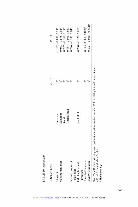
Tables 10A and B show student- and school-level covariate effects, respec-

tively, based on the multinomial logistic regression covariate model (see

Equations 7 and 8). Values in Table 10 are estimated regression coefficients.

As shown in Table 10, panel A, males were more likely than females to belong

to Class 1. American Indians or Alaskan Natives were more likely than Whites

to belong to Class 4; Asians, Asian Americans, or Pacific Islanders were less

likely than Whites to belong to Class 2; and African Americans, Mexicans, or

Mexican Americans were more likely than Whites to belong to Classes 2 and

4. Puerto Ricans and other Latinos or Latin Americans were more likely than

Whites to belong to Classes 2 and 4. At the school level (Table 10, panel B), only

household income and poverty levels (the higher value indicates higher poverty)

were significant among school-level covariates considered. Schools that have

higher household incomes and lower poverty levels were more likely to belong

to school Class 2.

Finally, the last five items on the test were examined as a group to determine

whether particular response patterns might emerge conditional on group


359



TA

BL

E10

Cova

riate

Eff

ects

for

Math

emati

csSec

tion

A.

Stu

den

tL

evel

G¼

1G¼

2G¼

3G¼

4

Inte

rcep

tK¼

10.3

80

(0.0

02,

1.0

17)*

0.1

33

(–0.1

66,

0.6

12)

0a

–0.5

87

(–0.9

00,

–0.1

58)*

K¼

2–0.5

90

(–0.9

29,

–0.2

50)*

–0.3

59

(–0.5

71,

–0.1

27)*

0a

–1.4

31

(–1.6

82,

–1.1

88)*

Gen

der

Fem

ale

–0.2

77

(–0.4

75,

–0.0

328)*

0.1

24

(–0.0

19,

0.2

79)

0a

0.1

24

(–0.0

19,

0.2

79)

Eth

nic

ity

No

resp

onse

–0.2

07

(–1.0

92,

0.5

46)

0.7

02

(0.0

77,

1.2

73)*

0a

2.1

65

(1.6

16,

2.6

56)*

Am

eric

anIn

dia

nor

Ala

ska

Nat

ive

–0.4

29

(–1.6

17,

0.7

57)

0.3

43

(–0.5

87,

1,2

53)

0a

1.0

40

(0.2

62,

1.8

56)*

Asi

an,

Asi

anA

mer

ican

,or

Pac

ific

Isla

nder

–0.3

03

(–0.6

08,

0.0

59)

–0.7

35

(–1.0

16,

–0.3

99)*

0a

–0.3

27

(–0.6

67,

0.0

08)

Bla

ckor

Afr

ican

Am

eric

an–0.1

23

(–0.6

08,

0.3

30)

1.5

02

(1.2

18,

1.7

75)*

0a

2.6

20

(2.3

53,

2.9

02)*

Mex

ican

or

Mex

ican

Am

eric

an

–0.6

12

(–1.5

55,

0.2

17)

1.3

84

(1.0

15,

1.7

73)*

0a

1.9

12

(1.5

97,

2.3

02)*

Puer

toR

ican

–0.4

96

(–1.4

92,

0.4

49)

1.1

72

(0.5

76,

1.8

52)*

0a

2.1

87

(1.6

22,

2.7

68)*

Oth

erH

ispan

ic,

Lat

ino,

or

Lat

inA

mer

ican

–0.4

43

(–1.0

61,

0.1

31)

1.2

56

(0.8

94,

1.5

84)*

0a

1.8

84

(1.5

44,

2.2

6)*

Oth

er–0.1

63

(–0.8

33,

0.4

27)

0.4

18

(�0.0

38,

0.8

43)

0a

1.0

75

(0.6

57,

1.4

73)*

*si

gnif

ican

tat

p¼

0.0

5.

360



TA

BL

E10

(conti

nued

)

B.

Sch

ool

Lev

elK¼

1K¼

2

Inte

rcep

tIn

terc

ept

0a

–1.1

92

(–2.8

59,

0.2

95)

Met

ropoli

tan

code

Suburb

an0

a0.0

88

(–0.5

78,

0.8

44)

Rura

l0

a0.2

87

(–0.5

60,

1.1

87)

Uncl

assi

fied

0a

–0.4

84

(–2.0

91,

1.0

89)

Sch

ool

enro

llm

ent

size

code

0a

0.2

76

(–0.2

95,

0.8

47)

Tit

leI

schoolw

ide

pro

gra

m

No

Tit

leI

0a

0.7

30

(–0.1

20,

0.8

10)

House

hold

inco

me

0a

0.1

45

(0.0

80,

0.1

80)*

Pover

tyle

vel

code

0a

–0.8

05

(–1.0

01,

–0.7

12)*

Note

:T

ype

IIla

bel

swit

chin

gac

ross

wit

hout

and

wit

hco

var

iate

model

s.95%

cred

ibil

ity

inte

rval

inpar

enth

eses

.

a.F

ixed

for

model

iden

tifi

cati

on.

*S

ignif

ican

tat

p.

361



membership. This was done for models with and without covariates. These five

items were gridded-in items and were classified as high difficulty in the item

descriptions. Several patterns of omitted responses were noted: 99900, 99909,

99990, and 99999 (where 0, 1, and 9 indicate incorrect, correct, and omitted

responses, respectively). No students assigned to Class 3, the high-ability group,

had any omitted responses. Students with 0s and 1s, that is, students who tried to

answer the question, were classified mostly into the average-and high-ability

groups.

Discussion

A MMixIRTM was described for modeling multilevel item response data at

both the student level and school level. The model developed in this study used

features of an IRT model, an unrestricted latent class model, and a multilevel

model. The student level of the model provides an opportunity to determine

whether latent classes exist that differ in their response strategies to answering

questions. Information at the school level can be used to reveal possible differ-

ences that might be due to curricular or pedagogical differences among latent

classes. In addition, a Bayesian solution was described for estimation of

the model parameters as implemented using the freely available software,

WinBUGS. A simulation study was presented to investigate the performance

of the model under some practical DIF testing conditions. Generated parameters

were recovered very well for the conditions considered. Use of MMixIRTM was

also illustrated with a standardized mathematics test.

The MMixIRTM makes it possible to describe differential item performance

of a target school using descriptions of student- and school-level characteristics

associated with the given school compared to characteristics associated with

other schools not in the same latent class as the target school. This description

can then be used to provide schools with a framework within which to compare

the results of their school with other schools in their latent class and in the other

latent classes. As an example, schools classified into the same latent class as the

target school (i.e., school-level Class 2) were characterized by lower Title I

enrollment, higher household income, lower poverty levels, and a predominance

of students in student-level latent Class 1. Students in each of the latent classes

were also characterized by differences in ability, as well as by differences in

response strategies, particularly at the end of the test. In the DIF example, pro-

viding a description of all schools that are members of the same school-level

latent class facilitated comparisons among latent classes and allowed for the pos-

sibility that there may be more than one comparison group.

In this study, the pairwise standardized item difficulty differences between

groups were used for DIF detection (Lord, 1980; Wright & Stone, 1979;

Zimowski et al., 1996) in the context of the HPD interval (Samuelsen, 2005,

2008; Samuelsen & Bradshaw, 2008). This procedure is only one of the ways

Cho and Cohen

362



of implementing a DIF analysis in a Rasch model. This method can yield DIF

inflation when DIF is asymmetrical (De Boeck, 2008; Wang, 2004). DIF is asym-

metrical if it is restricted to a subset of the items showing a mean difference in

difficulty between the two groups (De Boeck, 2008). The likelihood ratio test

(Thissen, Steinberg, & Wainer, 1988, 1993) is a more general model-based

approach. One issue that needs to be addressed in a MixIRTM DIF study is find-

ing anchor items for scale comparability across latent classes.

Information in Table 9 was used to characterize latent classes with respect to

item difficulty at both student and school levels. Information regarding item-

level content and surface characteristics of items would also be helpful for char-

acterizing patterns of responses in latent classes. Because of the secure nature of

the test, however, test content was not available for analysis in this study. Some

success has been shown, for example, using cognitive characteristics of mathe-

matics test items to explain differences between gender groups (Gallagher,

1998; Gallagher & DeLisi, 1994; Gallagher, Morley, & Levin, 1999). Similarly,

surface characteristics of items have been used to explain some gender DIF in

mathematics test items (Li, Cohen, & Ibarra, 2004). Cognitive skills have been

modeled to reflect basic features of items in the linear logistic test model (Fisher,

1983). Tatsuoka (1983) described a Q matrix to contain this information, the

entries of which indicate whether a particular cognitive skill is required by attri-

bute h in item i. Elements of the Q matrix, qih, are either 1, if attribute h is

required by item i, or 0, if it is not. One way this matrix can be incorporated into

the MMixIRTM is with the following linear structure:

bigk ¼X

h

bgkhqih; ð20Þ

where bgkh is the contribution to item difficulty required by attribute h for each

class, g and k.

The substantive usefulness of the MMixIRTM is based on the assumption that

the resulting latent classes represent discrete subpopulations and are not just sta-

tistical artifacts of nonnormality that may incidentally exist in the data (Bauer &

Curran, 2003). At the present time, little evidence exists indicating what schools

look like based on latent classes. Results of the simulation study suggest that the

findings of this study were not artifacts in that the algorithm was able to correctly

detect generated groups in the data. The resulting student- and school-level mix-

tures in the data examined in the empirical example, likewise, were clearly dis-

tinguishable in terms of ability levels, item difficulty profiles, student and school

demographic characteristics, and response patterns. When several factors deter-

mine a class, however, finding those factors that cause the DIF potentially may be

difficult.

In the MMixIRTM, as the number of school-level DIF items increases,

the characteristics of school-level latent classes should also change. That is, the

model rationale for constructing school-level latent classes is dependent on the


363



proportion of school-level DIF items. It may be that the number of non-DIF items

that are needed to anchor the construct across school-level mixtures be consid-

ered a substantive issue as well as a statistical one. In the empirical illustration,

we demonstrated that it was possible to obtain class-specific item difficulties for

each g and k and to express these on the same scale. No constraints were set that

required identifying non-DIF items across groups. The analysis needed to ensure

the meaning of g was the same or similar across classes after class-specific item

difficulties were obtained. In the example, item profiles were similar between the

same student-level latent classes across school-level latent classes. It appears, in

other words, that the construct characterized by class-specific item difficulties is

similar across school-level classes.

The second type of label switching, that is, switching among different replica-

tions of the same simulation conditions, was observed in the simulation study.

This type of label switching can be problematic (a) for checking convergence

using more than two chains, (b) for comparing student-level latent group mem-

bership across school-level latent classes (because the student-level probability

of mixtures is modeled for each school-level class), and (c) for comparing results

with and without covariates. The WinBUGS code developed for this study was

not designed to prevent the second type of label switching. Although this type

of label switching can be easily detected and taken care of in a simulation study,

it can be a serious problem with real data. The strategy used in this study to check

for this type of label switching was to investigate item difficulty profiles and

ability patterns for each school latent class to see whether the representation was

similar across school-level mixtures and to cross-tabulate group memberships to

find the dominant group.

Noninformative prior distributions for parameters were not considered for

two reasons. First of all, improper priors cannot be implemented in WinBUGS,

and second, attempts using diffuse priors resulted in a substantial number of

traps. The focus here was with the analysis of large-scale achievement data

having a hierarchical data structure, so that the effect of prior information was

likely negligible anyway. In this regard, the result with the WinBUGS code has

been shown to be comparable with the result with LatentGOLD syntax module

based on marginal maximum likelihood estimation (Vermunt & Magidson,

2007).

von Davier and Yamamoto (2007) have noted that MCMC typically requires

substantial computing time to obtain usable results. This is due, in part, to the use

of multiple starting points necessary with empirical data to determine whether

the algorithm has converged. For this reason, the amount of computing required

can sometimes be very large. In the case of the example in this study, 90 hours

were required for one condition in the simulation study and 121.5 hours were

required for the empirical study on a 3.0-GHz computer with 1 GB of RAM to

complete a single replication. Results such as this are not uncommon, and opera-

tional estimation of model parameters for long tests and very large samples using

Cho and Cohen

364



MCMC is clearly going to require either substantial computing resources or

development of speedier algorithms.

Appendix

WinBUGS Code Used for MMixIRTM

# 2 student-level class (G) with prior# 2 school-level class (K)with prior# J: the number of students# I: the number of items# T: the number of schools# g: group (i.e. student) membership at the student-level# gg (k): group (i.e., school) membership at the school-level# a: the SD of ability# b: item difficulty# eta: ability# mutg: the mean of abilitymodel{for (j in 1:J) {

for (i in 1:I) {r[j,i] <- resp[j,i]

}}# G¼2for (j in 1:J) {

for (i in 1:I) {logit(p[j,i]) <- a[g[j], gg[group[j]]] *eta[j]- b[i,g[j],gg[group[j]]]r[j,i]*dbern(p[j,i])

}}# Abilityfor (j in 1:J) {

eta[j]*dnorm(mutg[g[j],gg[group[j]]], 1)}mutg[1,1] <- 0mutg[2,1] * dnorm(0,1)mutg[1,2] * dnorm(0,1)mutg[2,2] * dnorm(0,1)

# SD of Abilityfor (g in 1:G2) {

for (k in 1:K2){a[g, k] * dnorm(0,1) I(0,)

}}# Student Levelfor (j in 1:N) {

g[j] * dcat(pi[gg[group[j]],1:G2])}for (k in 1:K2) {

for (g in 1:G2) {pi[k,g] <- delta[k,g] /sum(delta[k,])delta[k,g] * dgamma(alpha[g],1)

}

(continued )


365



Appendix (continued )

}# School Levelfor (t in 1:T){

gg[t] * dcat(pi1[1:K2])}for (k in 1:K2) {

pi1[k] <- delta1[k]/sum(delta1[1:K2])delta1[k] * dgamma(alpha1[k],1)

}# Item Difficultyfor (i in 1:T) {

for (g in 1:G2) {for (k in 1:K2){b[i,g,k]*dnorm(0,1)

}}}# Log-Likelihoodfor (j in 1:J) {

for (i in 1:I) {l[j,i]<-log(p[j,i])*r[j,i]þlog(1-p[j,i])*(1-r[j,i])

}}loglik <-sum(l[1:J,1:I])AIC <- -2*(loglik - np)BIC <- -2*loglik þ np*log(N)}# Initial Value of School-Level Group Membershiplist(gg¼c(1,2,1,2,1,2,1,2,1,2,1,2,1,2,1,2,1,2,1,2,1,2,1,2,1,2,1,2,1,2,1,2,1,2,1,2,1,2,1,2,1,2,1,2,1,2,1,2,1,2,1,2,1,2,1,2,1,2,1,2,. . .

1,2,1,2,1,2,1,2,1,2,1,2,1,2,1,2,1,2,1,2,1,2,1,2,1,2,1,2,1,2,1,2,1,2,1,2,1,2,1,2))

# Input Data# 25 studentslist(J¼8000, I¼40, T¼320, G2¼2, K2¼2, np¼169, alpha¼c(1,1),alpha1¼c(1,1),group¼c(1,1,1,1,1,1,1,1,1,1,1,1,1,1,1,1,1,1,1,1,1,1,1,1,1,2,2,2,2,2,2,2,2,2,2,2,2,2,2,2,2,2,2,2,2,2,2,2,2,2,3,3,3,3...),resp¼structure(.Data¼c(1.0,1.0,1.0,1.0,1.0,. . .

1.0,0.0,0.0,0.0,0.0),.Dim ¼ c(8000,40)))

References

Akaike, H. (1974). A new look at the statistical model identification. IEEE Transactions

on Automatic Control, 19, 716–723.

Cho and Cohen

366



Asparouhov, T., & Muthen, B. (2008). Multilevel mixture model. In G. R. Hancock & K.

M. Samuelsen (Eds.), Advances in latent variable mixture models (pp. 25–51). Green-

wich, CT: Information Age Publishing, Inc.

Bates, D., & Debroy, S. (2004). Linear mixed models and penalized least squares. Journal

of Multivariate Analysis, 91, 1–17.

Bauer, D. J., & Curran, P. J. (2003). Distributional assumptions of growth mixture models:

Implications for overextraction of latent trajectory classes. Psychological Methods, 8,

338–363.

Bolt, D. M., Cohen, A. S., & Wollack, J. A. (2001). A mixture item response for multiple-

choice data. Journal of Educational and Behavioral Statistics, 26, 381–409.

Bolt, D. M., Cohen, A. S., & Wollack, J. A. (2002). Item parameter estimation under con-

ditions of test speededness: Application of a Mixture Rasch model with ordinal con-

straints. Journal of Educational Measurement, 39, 331–348.

Box, G. E. P., & Tiao, G. C. (1973). Bayesian inference in statistical analysis. Reading,

MA: Addison-Wesley.

Bryk, A. S., & Raudenbush, S. W. (1988). Toward a more appropriate conceptualization

of research on school effects: A three-level hierarchical linear model. American Journal

of Education, 97, 65–108.

Cohen, A. S., & Bolt, D. M. (2005). A mixture model analysis of differential item func-

tioning. Journal of Educational Measurement, 42, 133–148.

Cohen, A. S., Cho, S.-J., & Kim, S.-H. (2005, April). A mixture testlet model for educa-

tional tests. Paper presented at the annual meeting of the American Educational

Research Association, Montreal, Canada.

Cohen, A. S., Gregg, N., & Deng, M. (2005). The role of extended time and item content on

a high-stakes mathematics test. Learning Disabilities Research & Practice, 20, 225–233.

Congdon, P. (2003). Applied Bayesian modeling. New York: Wiley.

Dayton, C. M., & Macready, G. B. (1988). Concomitant variable latent-class models.

Journal of the American Statistical Association, 83, 173–178.

DeAyala, R. J., Kim, S.-H., Stapleton, L. M., & Dayton, C. M. (2002). Differential item

functioning: A mixture distribution conceptualization. International Journal of Testing,

2, 243–276.

De Boeck, P. (2008). Random item IRT models. Psychometrika, 73, 533–559.

Fisher, G. H. (1983). Logistic latent trait models with linear constraints. Psychometrika,

48, 3–26.

Fox, J.-P. (2005). Multilevel IRT using dichotomous and polytomous response data.

British Journal of Mathematical and Statistical Psychology, 58, 145–172.

Fox, J.-P., & Glas, C. (2001). Bayesian estimation of a multilevel IRT model using Gibbs

sampling. Psychometrika, 66, 271–288.

Gallagher, A. M. (1998). Gender and antecedents of performance in mathematics testing.

Teachers College Record, 100, 297–314.

Gallagher, A. M., & DeLisi, R. (1994). Gender differences in scholastic aptitude

test-mathematics problem solving among high ability students. Journal of Educational

Psychology, 86, 204–211.

Gallagher, A. M., Morley, M. E., & Levin, J. (1999). Cognitive patterns of gender differ-

ences on mathematics admissions tests. In Graduate Record Examinations FAME

Report (pp. 4–11). Princeton, NJ: Education Testing Service.


367



Gelman, A., Carlin, J. B., Stern, H. S., & Rubin, D. B. (2003). Bayesian data analysis

(2nd ed.). Boca Raton, FL: Chapman & Hall/CRC.

Gelman, A., & Rubin, D. B. (1992). Inference from iterative simulation using multiple

sequences. Statistical Science, 7, 457–472.

Geweke, J. (1992). Evaluating the accuracy of sampling-based approaches to calculating

posterior moments. In J. M. Bernardo, J. O. Berger, A. P. Dawid, & A. F. M. Smith

(Eds.), Bayesian statistics (Vol. 4, pp. 169–194). UK: Oxford University Press.

Goldstein, H. (1987). Multilevel models in education and social research. London:

Charles Griffin and Co.

Jordan, M. I., & Jacobs, R. A. (1992). Hierarchies of adaptive experts. In J. Moody,

S. Hanson, & R. Lippmann (Eds.), Advances in neural information processing systems

(Vol. 4, pp. 985–993). San Mateo, CA: Morgan Kaufmann.

Kamata, A. (2001). Item analysis by the hierarchical generalized linear model. Journal of

Educational Measurement, 38, 79–93.

Li, Y., Cohen, A. S., & Ibarra, R. A. (2004). Characteristics of mathematics items asso-

ciated with gender DIF. International Journal of Testing, 4, 115–136.

Longford, N. T. (1993). Random coefficient models. New York: Oxford University Press.

Lord, F. M. (1980). Applications of item response theory to practical testing problems.

Hillsdale, NJ: Lawrence Erlbaum.

Maier, K. S. (2001). A Rasch hierarchical measurement model. Journal of Educational

and Behavioral Statistics, 26, 307–330.

Maier, K. S. (2002). Modeling incomplete scaled questionnaire data with a partial credit hier-

archical measurement model. Journal of Educational and Behavioral Statistics, 27, 271–289.

McLachlan, G., & Peel, D, (2000). Finite mixture models. New York: Wiley.

Mislevy, R. J., & Verhelst, N. (1990). Modeling item responses when different subjects

employ different solution strategies. Psychometrika, 55, 195–215.

Rabe-Hesketh, S., Skrondal, A., & Pickles, A. (2004). Generalized multilevel structural

equation modeling. Psychometrika, 69, 167–190.

Raftery, A. L., & Lewis, S. (1992). How many iterations in the Gibbs sampler? In

J. M. Bernardo, J. O. Berger, A. P. Dawid, & A. F. M. Smith (Eds.), Bayesian statistics

(Vol. 4, pp. 763–773). UK: Oxford University Press.

Raudenbush, S. W., & Bryk, A. G. (2002). Hierarchical linear models: Applications and

data analysis methods (2nd ed.). Thousand Oaks, CA: Sage.

Richardson, S., & Green, P. J. (1997). On Bayesian analysis of mixtures with an unknown

number of components (with discussion). Journal of the Royal Statistical Society,

Series B, 59, 731–792. Correction (1998). Journal of the Royal Statistical Society

Series, Series B, 60, 661.

Rost, J. (1990). Rasch models in latent classes: An integration of two approaches to item

analysis. Applied Psychological Measurement, 14, 271–282.

Rost, J. (1997). Logistic mixture models. In W. J. van der Linden & R. K. Hambleton

(Eds.), Handbook of modern item response theory (pp. 449–463). New York:

Springer.

Samuelsen, K. M. (2005). Examining differential item functioning from a latent class

perspective. Unpublished doctoral dissertation, University of Maryland, College

Park.

Cho and Cohen

368



Samuelsen, K. M. (2008). Examining differential item functioning from a latent class

perspective. In G. R. Hancock & K. M. Samuelsen (Eds.), Advances in latent variable

mixture models (pp. 67–113). Charlotte, NC: Information Age Publishing.

Samuelsen, K. M., & Bradshaw, L. (2008). The credibility interval method for the

detection of DIF within a Bayesian framework. Paper presented at the annual meeting

of the National Council on Measurement in Education, New York City.

Schwarz, G. (1978). Estimating the dimension of a model. Annals of Statistics, 6, 461–464.

Smith, B. (2004, April). Bayesian output analysis program (BOA) (Version 1.1.2 for R and

S-PLUS) [Computer program]. Iowa City: University of Iowa, Department of Biostatistic.

Spiegelhalter, D., Thomas, A., & Best, N. (2003). WinBUGS (Version 1.4) [Computer

program]. Cambridge UK: MRC Biostatistics Unit, Institute of Public Health.

Stephens, M. (2000). Dealing with label switching in mixture models. Journal of the

Royal Statistical Society, Series B, 62, 795–809.

Tatsuoka, K. K. (1983). Rule space: An approach for dealing with misconceptions based

on item response theory. Journal of Educational Measurement, 20, 345–354.

Thissen, D., Steinberg, L., & Wainer, H. (1988). Use of item response theory in the study

of group differences in trace lines. In H. Wainer & H. I. Braun (Eds.), Test validity

(pp. 147–169). Hillsdale, NJ: Lawrence Erlbaum.

Thissen, D., Steinberg, L., & Wainer, H. (1993). Detection of differential item functioning

using the parameters of item response models. In P. W. Holland & H. Wainer (Eds.),

Differential item functioning (pp. 67–113). Hillsdale, NJ: Lawrence Erlbaum

Associates.

Vermunt, J. K. (2003). Multilevel latent class models. Sociological Methodology, 33,

213–239.

Vermunt, J. K. (2007a). Multilevel mixture item response theory models: An application

in education testing. ISI 2007 Proceedings.

Vermunt, J. K. (2007b). A hierarchical model for clustering three-way data sets. Compu-

tational Statistics & Data Analysis, 51, 5368–5376.

Vermunt, J. K., & Magidson, J. (2005). Technical guide for Latent GOLD 4.0: Basic and

advanced. Belmont, MA: Statistical Innovations Inc.

Vermunt, J. K., & Magidson, J. (2007). Latent GOLD 4.5 syntax module [Computer pro-

gram]. Belmont, MA: Statistical Innovations Inc.

von Davier, M., & Yamamoto, K. (2007). Mixture-distribution and HYBRID Rasch mod-

els. In M. von Davier & C. H. Carstensen (Eds.), Multivariate and mixture distribution

Rasch models (pp. 99–115). New York: Springer.

Wang, W.-C. (2004). Effect of anchor item methods on the detection of differential item

functioning within the family of Rasch models. Journal of Experimental Education, 72,

221–261.

Wollack, J. A., Cohen, A. S., & Wells, C. S. (2003). A method for maintaining scale sta-

bility in the presence of test speededness. Journal of Educational Measurement, 40,

307–330.

Wright, B. D., & Stone, M. H. (1979). Best test design. Chicago: Measurement, Evalua-

tion, Statistics, and Assessment Press.

Yamamoto, K., & Everson, H. (1997). Modeling the effects of test length and test time on

parameter estimation using the HYBRID model. In J. Rost & R. Langenheine (Eds.),


369



Applications of latent trait and latent class models in the social sciences. New York,

NY: Waxmann.

Zimowski, M. F., Muraki, E., Mislevy, R. J., & Bock, R. D. (1996). Multiple-group IRT

analysis and test maintenance for binary items. Chicago: Scientific Software.

Authors

SUN-JOO CHO is an assistant professor at Peabody College of Vanderbilt University,

Hobbs 213A 230 Appleton Place, Nashville, TN 37203; e-mail: [email protected].

Her research interests are the modeling of item response data using item response the-

ory and its parameter estimation.

ALLAN S. COHEN is a professor at University of Georgia College of Education, 570

Aderhold Hall, Athens, GA30602; email: [email protected]. His research interests are

applied statistics and psychometric theory.

Manuscript received April 29, 2008

Revision revised May 16, 2009

Accepted August 18, 2009

Cho and Cohen

370



journal of educational and behavioral ... - moodle.eduhk.hk

Documents