Journal of Financial Economics 134 (2019) 617–646

Contents lists available at ScienceDirect

Journal of Financial Economics

journal homepage: www.elsevier.com/locate/jfec

Time-varying ambiguity, credit spreads, and the levered

equity premium

�

Zhan Shi

PBC School of Finance, Tsinghua University, 43 Chengfu Road, Haidian District, Beijing 10 0 083, China

a r t i c l e i n f o

Article history:

Received 1 September 2015

Revised 26 June 2018

Accepted 31 July 2018

Available online 11 May 2019

JEL classification:

E43

E44

G12

G13

G33

Keywords:

Ambiguity

Credit spreads

Equity premium

a b s t r a c t

This paper studies the effects of time-varying Knightian uncertainty (ambiguity) on asset

pricing in a Lucas exchange economy. Specifically, it considers a general equilibrium model

where an ambiguity-averse agent applies a discount rate that is adjusted not only for the

current magnitude of ambiguity but also for the risk associated with its future fluctuations.

As such, both the ambiguity level and volatility help to raise the asset premiums and ac-

commodate richer dynamics of asset prices. Based on a novel empirical measure of the

ambiguity level, the estimated model can capture the empirical levels of corporate credit

spreads and the equity premium while endogenously matching the historical default prob-

ability. More importantly, the model-implied credit spread and equity price-dividend ratio

perform remarkably in tracking the time variations in their historical counterparts.

© 2019 Elsevier B.V. All rights reserved.

1. Introduction

As long as investors have access to multiple asset

classes, prices of these assets across markets ought to

equal their expected cash flows discounted by the same

� I am indebted to my committee, Jingzhi Huang (Chair), Heber

Farnsworth, Olesya Grishchenko, Joel Vanden, and Jared Williams. I also

thank Daniele Bianchi, Hui Chen, Paul Ehling, Michael Gallmeyer, Lorenzo

Garlappi, Jean Helwege, Jianfeng Hu, Ravi Jagannathan, Anahit Mkrtchyan,

Ivan Shaliastovich, Jess Smith, Jianfeng Yu, Xudong Zeng, an anonymous

referee, and seminar participants at the 2014 WFA Annual Meetings

(Monterey), the 2016 China International Conference in Finance (Xiamen),

BI Norwegian Business School, Ohio State University, Penn State Univer-

sity, Tsinghua University, and University of Virginia (McIntire) for helpful

comments and suggestions. I am also grateful to John Graham for pro-

viding his estimates of the corporate marginal tax rates. A previous draft

was circulated under the name “Time-Varying Ambiguity and Asset Pric-

ing Puzzles”. Research support from the Smeal summer dissertation grant

is gratefully acknowledged.

E-mail address: shizh@pbcsf.tsinghua.edu.cn

https://doi.org/10.1016/j.jfineco.2019.04.013

0304-405X/© 2019 Elsevier B.V. All rights reserved.

stochastic discount factor. Perhaps the best embodiment of

this idea of consistent cross-market pricing is the struc-

tural approach to credit risk modeling, as pioneered by

Black and Scholes (1973) and Merton (1974) . This approach

treats corporate debt and equity as contingent claims writ-

ten on the same productive assets and thus builds a direct

link not only between their discount-rate risks but also be-

tween their cash-flow risks. For structural credit models to

be fruitfully used, especially in terms of inferring risk pre-

miums across stock and bond markets, 1 they need to si-

multaneously generate equity premium and credit spreads

that are consistent with the data. Empirically, however, a

controversy has arisen about their ability to do so with

1 For example, Campello et al. (2008) and van Zundert and Driessen

(2018) use corporate yield spreads to construct an ex ante measure of

the equity premium, and Elkamhi and Ericsson (2008) take the opposite

direction by estimating bond risk premiums using equity data.

618 Z. Shi / Journal of Financial Economics 134 (2019) 617–646

5 In addition, given that corporate defaults tend to cluster when the

economic outlook becomes unclear, the liquidation process can be partic-

reasonable parameters matching historical default experi-

ence. 2

In this paper, we show that temporal variation in am-

biguity (Knightian uncertainty) 3 carries important impli-

cations for the joint valuation of debt and equity; it

creates an additional uncertainty channel that helps struc-

tural models match the historical equity premium and

credit spreads while endogenously generating reasonable

default rates. The role of time-varying ambiguity is fulfilled

through its twofold effects on (uncertainty-adjusted) dis-

count rates.

First, consider an exchange economy where a represen-

tative agent holds multiple priors ( Gilboa and Schmeidler,

1989 ) about aggregate consumption dynamics. To make de-

cisions robust to model misspecifications, the ambiguity-

averse agent optimally evaluates investments according to

the prior that leads to the lowest expected utility. This

“worst-case” evaluation brings about a first-order effect

of ambiguity on discount rates, wherein the magnitude is

determined by the difference between the true expected

growth rate and the worst-case belief used to price as-

sets. Second, if the set of priors is updated over time, the

uncertainty about future ambiguity levels also permits a

second-order effect on discount rates, in the sense that the

magnitude of this effect is bound to the second mo-

ment (volatility) of the ambiguity process. In the model

proposed in this paper, the presence of asymmetry in am-

biguity volatility, 4 in conjunction with the agent’s prefer-

ence for early resolution of uncertainty, implies that the

second-order effect works in the same direction as the

first-order effect: a rise in the degree of ambiguity in-

creases discount rates. These two effects jointly create a

strong, negative correlation between the pricing kernel and

asset valuation ratios, which per se accounts for a sizable

unlevered equity premium.

However, the most interesting implication of the

uncertainty-adjusted discount rates arises from endoge-

nous default decisions. Specifically, an (positive) ambigu-

ity shock would lower the present value of a given path of

2 The key to this controversy is the definition of “reasonable parame-

ter values.” Huang and Huang (2012) find that various structural models,

once calibrated to match historical default and recovery rates as well as

the equity premium, underpredict corporate yield spreads (especially for

investment-grade bonds). This finding is referred to as the “credit spread

puzzle.” Taking the view that the level of yield spreads due to non-credit

factors is of similar magnitude for Aaa and Baa bonds, other studies ( Chen

et al., 2009; McQuade, 2016; Du et al., 2018 ) show a similar puzzle in

Baa-Aaa yield spreads. On the other hand, David (2008) and Bhamra et al.

(2010) study the impact of convexity bias on the calculation of modeled

credit spreads, suggesting that the credit spread puzzle may not be as se-

vere as documented by Huang and Huang (2012) . Furthermore, Feldhütter

and Schaefer (2018) criticize the practice of calibrating structural mod-

els to historical default frequencies by rating and maturity groups; they

propose a new calibration approach to make the Black-Cox model gener-

ate investment-grade credit spreads that are consistent with the empirical

counterparts. 3 Ambiguity refers to the situation in which the decision-maker is un-

certain about the probability law governing the state process. For notional

convenience, in this paper we refer to uncertainty as both risk and ambi-

guity, unless Knightian uncertainty, model uncertainty, or subjective un-

certainty is otherwise used in that context. 4 Asymmetric volatility refers to the fact that an increase in volatility

follows a previous rise in the ambiguity level.

future cash flows, and thus leans shareholders toward ex-

ercising their options to default, even if there is no news of

the firm’s fundamentals. Therefore, time-varying ambiguity

introduces a novel linkage from discount rates to corpo-

rate default timing. On the one hand, it exposes investors

to great default risk exactly in the periods associated with

high market prices of risk 5 ; thus, high yield spreads must

be demanded for investing in corporate bonds. On the

other hand, equity holders are more likely to lose their

cash flow rights and bear the deadweight losses exactly

when their marginal utility is high. This risk channel em-

beds an additional component in the uncertainty premium

on levered equity, making it greater than that on the un-

levered asset.

Few examples of general equilibrium models succeed in

explaining the equity premium and credit spreads in a uni-

fied framework: Chen et al. (2009 , CCG hereinafter) build

on the habit-formation model of Campbell and Cochrane

(1999) ; Bhamra et al. (2010 , BKS hereinafter), and Chen

(2010) use a theoretical framework in the spirit of Bansal

and Yaron (2004) that incorporates regime switching. 6 This

paper departs from these existent studies in three impor-

tant aspects.

1. While these studies aim to explain the equity pre-

mium and credit spreads with macroeconomic risk, 7

our explanation is based on time-varying Sharpe ratios

that are driven by changes in the ambiguity level. This

key difference gives our model two important advan-

tages in fitting not only the average level but also the

time series of historical credit spreads. First, it entitles

our model to accounting for variations in asset premi-

ums above and beyond what are captured by the busi-

ness cycle. The economic intuition is that an ambiguity

shock can lead to a large reaction in the marginal rate

of substitution, even without news about the economic

ularly costly during such times. Empirically, we also find that high costs

of default are associated with high ambiguity levels. Consequently, the

pricing kernel shows an even stronger (positive) covariance with expected

default losses compared to the case in which it only comoves with the

default probability, further magnifying the model-implied credit spreads. 6 Christoffersen et al. (2017) combine two risk channels, habit forma-

tion and rare disaster, to capture the empirical level and volatility of

credit spreads, as well as stylized facts in the option market. However,

they embed a reduced-form model (rather than a structural one) of credit

risk inside their representative-agent consumption-based model. Other

studies attempting to reconcile the credit spread puzzle include David

(2008) , Du et al. (2018) , McQuade (2016) , Albagli et al. (2013) , and Chen

et al. (2018) . These models either are not set in general equilibrium or do

not consider the equity premium. 7 As highlighted in CCG (2009), the key ingredient in all three mod-

els is the market Sharpe ratio that varies with macroeconomic condi-

tions. However, Huang and Huang (2012) advise caution when linking the

credit spread puzzle to recession risk since “there is no clear evidence

yet that corporate bond defaults, especially on investment-grade bonds,

are strongly correlated with business cycles.” The reason is that histori-

cal variation in the aggregate default rate is almost completely driven by

speculative-grade issuers, whereas the credit spread puzzle mainly con-

cerns investment-grade bonds. As a result, countercyclical default rates

do not lend empirical validity to macro-risk-based explanations for the

credit spread puzzle. In other words, one needs to assess the model’s ex-

planatory power for the time variation of credit spreads, rather than that

of default rates, when trying to validate the proposed risk channels.

Z. Shi / Journal of Financial Economics 134 (2019) 617–646 619

9 Using observations of credit default swap (CDS) spreads on financial

institutions, Boyarchenko (2012) estimates a robust control model to back

out the implied amount of ambiguity during the subprime mortgage cri-

sis. Since her model does not adopt the structural approach to modeling

credit risk and is not calibrated to historical default rates, it does not carry

implications for the credit spread controversy. 10 Epstein and Schneider (2003) draw a head-to-head comparison be-

tween the robust control and recursive multiple-priors models. What

most distinguishes these modeling approaches is the updating rules im-

posed for the set of priors. To ensure dynamic consistency, multiplier

preferences need a form of axiom that differs from the rectangularity

employed by multiple-priors models. This form of axiom is provided by

Maccheroni et al. (2006) . Besides the multiple priors and multiplier util-

fundamentals. Second, it allows for time variations in

both the market prices of uncertainty (the first-order

effect) and the quantities of uncertainty (the second-

order effect). 8 The resultant flexibility explains why our

model outperforms existing ones in its time-series pre-

dictions.

2. Unlike these previous studies, which focus exclusively

on investment-grade issuers as inspired by Huang and

Huang (2012) ’s findings, we examine the credit spreads

of high-yield bonds as well. The latter is equally im-

portant in examining the credit spread controversy

because hypothetically we could reproduce the ob-

served level of investment-grade spreads by imposing

extremely high Sharpe ratios. But if the resulting model

were to overpredict speculative-grade yield spreads,

then it would merely create a “credit spread puzzle” in

the other direction. With a reasonable firm-level cali-

bration, our model can match empirical credit spreads

across all rating classes.

3. Beyond the momentous aspects of asset prices, this

paper also extensively studies their dynamic proper-

ties, which have not drawn sufficient attention in ex-

isting works on the credit spread controversy. Specif-

ically, our model is able to reproduce the following

empirical regularities: the procyclical variation of price-

dividend ratios, the countercyclical variation of credit

spreads, the long-horizon predictability of excess equity

returns and credit spreads, and their weak correlations

with macroeconomic fundamentals. These stylized facts

are indeed reflections of the same economic mecha-

nism, which is at the core of the model: time variation

in the pricing kernel is directly linked with the cash

flow risks of corporate securities through time-varying

ambiguity.

With respect to implementation, an important advan-

tage of our model is that the key driving variable, the

level of ambiguity, is measurable. This facilitates our data-

driven estimation of model parameters that does not in-

volve market data. Specifically, we construct a novel mea-

sure of the economy-wide level of ambiguity by using

survey forecasts. Consistent with our model’s implication,

higher ambiguity levels forecast higher market premiums

on a broad set of assets, including equities, corporate

bonds, and Treasury bonds. This ambiguity measure also

exhibits a positive correlation with the historical corpo-

rate default rate, consistent with the model’s prediction.

To further test the empirical plausibility of the proposed

economic mechanism, we estimate the default boundary

with a sample of defaulting bond issuers and find that the

ambiguity measure is highly significant in explaining the

estimated boundary (with the expected sign). This finding

substantiates the key theoretical implication that ambigu-

ity affects the default probability by moving the default

barrier.

8 In contrast, while models of CCG (2009), Chen (2010), and BKS (2010)

imply time-varying premiums as well, either the market prices of risks or

the quantities of risks are held constant in their models. Le and Singleton

(2010, 2013) firstly make this observation and point out the limitations

resulting from these specifications.

This paper also contributes to a growing body of litera-

ture that studies representative-agent asset pricing in the

presence of Knightian uncertainty. Our modeling of am-

biguity aversion builds on recursive multiple-priors util-

ity introduced and axiomatized by Epstein and Wang

(1994) , Chen and Epstein (2002) , and Epstein and Schnei-

der (2003) . We demonstrate that our specification of time-

varying ambiguity can be interpreted as a reduced form

of models of learning under ambiguity, as developed in

Epstein and Schneider (20 07, 20 08) and Illeditsch (2011) .

While these studies focus on model implications for the

equity market, the multiple-priors preferences are also ap-

plied to other asset classes ( Gagliardini et al., 2009; Ilut,

2012 ). However, the linkage of ambiguity aversion to the

credit spread controversy has not yet been examined in the

literature. 9

Outside the multiple-priors framework, a few theo-

retical works also accommodate time-varying ambiguity;

these studies employ a different approach to modeling am-

biguity aversion—multiplier (robust-control-inspired) util-

ity ( Hansen and Sargent, 2001; Anderson et al., 2003 ),

which defines the size of ambiguity in terms of relative

entropy. 10 Maenhout (2004) proposes an ambiguity-based

extension of Merton (1969, 1971, 1973) ’s optimality and

equilibrium theories and allows the tolerated entropy de-

viation to vary with the agent’s wealth. In their decompo-

sition of asset premiums into risk and (Knightian) uncer-

tainty components, Anderson et al. (2009) break the tight

link between ambiguity and wealth by letting the former

depend on other state variables as well. Targeting anoma-

lies in the option market, the model by Drechsler (2013) is

most closely related to ours in the sense that the ambigu-

ity level is also explicitly modeled as a separate stochas-

tic process. To fully capture properties of equity and op-

tion prices, as well as the variance premium, he allows for

“model uncertainty over a richer set of economic dynamics

than have been possible in previous applications of robust

control.”11 Consequently, ambiguity operates through mul-

tiple channels, and it is difficult to disentangle the impor-

tance of one channel from that of another. In contrast, our

parsimonious model focuses on one channel—Knightian

ity, there is a third type of preference model that describes ambiguity-

averse behavior called “smooth ambiguity” preferences ( Klibanoff et al.,

20 05; 20 09 ). Epstein and Schneider (2010) provide a comprehensive re-

view of the three alternative frameworks. 11 Drechsler (2013) ’s model features a predictable (long-run) component

and stochastic volatility in consumption growth, and he incorporates large

jumps in these two driving state processes. The agent in his model is con-

cerned about model misspecification with respect to all four components.

620 Z. Shi / Journal of Financial Economics 134 (2019) 617–646

V

uncertainty about expected consumption growth

12 —which

is absent in Drechsler (2013) ’s model.

The remainder of our paper is organized as follows. In

Section 2 , we introduce the model and characterize the

valuation of different assets in equilibrium. Section 3 de-

scribes how we measure economy-level ambiguity and il-

lustrates the empirical relevance of the proposed ambigu-

ity measure. Section 4 outlines the model estimation and

discusses quantitative implications on asset pricing puz-

zles. Section 5 presents our conclusions.

2. Model framework

In this section, we build a general equilibrium model

where the representative investor is uncertain about the

correct probability laws governing the state process. We

then allow Knightian uncertainty to vary in intensity over

time and derive relevant testable implications on equity

premium and credit spreads.

2.1. Modeling ambiguity aversion

Consider a measurable state space (�, F ) where each

F t ∈ F can be identified with a partition of �. Given a

probability measure P , F t is the σ -field generated by a

d -dimensional Brownian motion B t defined on (�, F , P ) .

Suppose that the representative decision-maker does not

know the true probability measure P 0 and ranks uncer-

tain consumption streams C = { C t } ∞

t=0 , where C t : � → R

is F t -measurable. To model preferences in the presence of

uncertainty, we adopt the structure of recursive multiple

priors:

∗t = min

P∈ P

�E P

[ ∫ ∞

t

f (C s , V

P s ) ds | F t

] , (1)

where the set P of priors on (�, F ) is constructed by

means of Girsanov transformation. In particular, we can

define the Radon–Nikodym derivative ( Z ) of P with re-

spect to the reference measure P 0 through a density gen-

erator ( ϑt ): 13

dZ ϑ t = −Z ϑ t ϑ t dB t , Z ϑ 0 = 1 (2)

Z ϑ t = exp

{−1

2

∫ t

0

| ϑ s | 2 ds −∫ t

0

ϑ s dB t

}, (3)

where B t is a Brownian motion under P 0 . It follows that the

generated measure P ϑ (ω) = Z(ω ) P 0 (ω ) is equivalent to P 0 .

This recursive multiple-priors model (1) –(3) is proposed

and axiomatized by Chen and Epstein (2002) , who prove

the existence and uniqueness of the solution to Eq. (1) . 14

12 Maenhout (2004) argues that the first moments of state variables are

more difficult to estimate than the second moments. 13 We assume that the regularity conditions, as specified in Appendix D

of Duffie (2001) , are satisfied so that Z ϑ t is a martingale under P 0 . 14 This well-established framework enables us to fully exploit the ana-

lytical power afforded by the continuous time. Its discrete-time version is

first put forth by Epstein and Wang (1994) , and the axiomatic foundations

are provided by Epstein and Schneider (2003) .

In a pure diffusion environment, ambiguity concerns

whether B t is a Brownian motion. 15 In other words, a

change of measure from P 0 to any P ∈ P affects only the

drift function of the utility continuation process. To be

more precise, the martingale representation theorem im-

plies that the utility process under P 0 can be written as

the solution to the backward stochastic differential equa-

tion ( Duffie and Epstein, 1992 ):

d V

P 0 t = − f (C t , V

P 0 t ) d t + σv ,t d B t . (4)

With the multiple-priors utility, the decision-maker’s acts

reflect her worst-case belief. Employing the Girsanov the-

orem, Chen and Epstein (2002) prove that B ∗t =

∫ t 0 ϑ

∗s ds +

B t is a Brownian motion under the worst-case measure,

where ϑ

∗s = max ϑ∈ � ϑ s .

Under Duffie and Epstein (1992) ’s parameterizations of

recursive preference, the aggregator function f takes the

form

f (C, V ) = βθV

[ (C

((1 − γ ) V ) 1

1 −γ

)1 − 1 ψ

− 1

]

, (5)

where β > 0 is the rate of time preference, γ � = 1 is the co-

efficient of relative risk aversion, and ψ � = 1 is the elastic-

ity of intertemporal substitution (EIS). 16 It follows that the

stochastic control problem is to find an optimal consump-

tion strategy c ∗ to maximize Eq. (1) :

J t = max C∈A

min

P∈ P

�E P

[ ∫ ∞

t

f (C s , V

P s ) ds | F t

] , (6)

where C ∈ A denotes that the control process { C t } is admis-

sible. Market clearing implies that the representative agent

takes up aggregate consumption (i.e., c ∗t = C t ).

2.2. Belief sets and ambiguity shocks

The dynamics of consumption growth are specified as a

diffusion process with time-varying drift:

dC t

C t = μc,t d t + σc d B C,t , (7)

where the sequence { μc,t } is unknown to the representa-

tive agent. The agent, who observes the realized C t , but

not its drift and diffusion terms separately, is unable to

tell whether an unexpected low realization of consumption

growth (or even a decline) is due to a worsening economic

state or just due to bad luck. The ambiguous component

in Eq. (7) is manifested in a further layer of incomplete

knowledge: the agent is only informed about the limiting

distribution of μc,t but holds little clue about its model

specification. More specifically, the empirical distribution

of μc,t is known to converge to N( μ, σ 2 μ) and be indepen-

dent of B C,t . On the other hand, the agent cannot disen-

tangle the true data-generating process (DGP) of μc,t from

15 Liu et al. (2005) and Drechsler (2013) consider agents who exhibit

ambiguity aversion toward jumps in the level or in the expected (long-

run) component of consumption growth. 16 γ and ψ jointly determine the attitude toward temporal resolution of

uncertainty. Because the recursive multiple-priors utility, per se, is neutral

about the timing of the resolution of uncertainty ( Strzalecki, 2013 ), the

agent’s temporal attitudes can be modeled separately with Eq. (5) , which

is the continuous-time version of Kreps–Porteus preferences.

Z. Shi / Journal of Financial Economics 134 (2019) 617–646 621

17 In our model, the exogenous state of the economy is summarized

by the pair ( C t , A t ). Therefore, the density generators are technically

two-dimensional, that is, ϑ ∗t = (A t /σc , 0) . This specification indicates that

the agent feels uncertain only about the consumption dynamics and not

about the ambiguity itself. The implicit assumption is that dispersion of

professional forecasts is considered to be plausibly reflecting uncertainty

about what the right model of the futures is, and the representative agent

infers the dynamics of ambiguity from measures of forecast dispersion, as

we will do in Section 3.1 from the perspective of econometricians. For ex-

ample, suppose that in the current period, experts, whose opinions are

sampled and aggregated by the agent to form her own belief set, are

in closer agreement about the future path of consumption growth than

they were in the last period. Consequently, the agent moves closer to-

ward thinking in terms of a single probability measure and knows that

the increased confidence in probability assessments is triggered by lower

forecast dispersion. Drechsler (2013) considers an extended specification

in which there is Knightian uncertainty about the dynamics of the size of

ambiguous beliefs.

a large family of possible processes, whose limiting distri-

butions are identical to that of an i.i.d. normal stochastic

process with mean μ and variance σ 2 μ, even after many

observations of C t .

As discussed by Epstein and Schneider (2007) , the mul-

tiplicity of probability measures in Eq. (1) indicates that

the agent “has modest (or realistic) ambitions about what

she can learn.” In our model setup, it captures the ambigu-

ous component μc,t , which is too poorly understood to be

theorized about. In response to this model uncertainty, the

agent forms a set of beliefs about expected consumption

growth at time t . We parameterize this set by an interval

centered around the long-run mean μ,

μP

c,t ∈ [ μ − A t , μ + A t ] , A t ≥ 0 , (8)

because to the agent, the observed consumption growth is

indistinguishable from a realization of geometric Brownian

motion,

dC t

C t = μd t + σg d B C,t , (9)

where σg =

√

σ 2 μ + σ 2

c . It follows that A t in Eq. (8) captures

the level of ambiguity about the expected growth rates.

That is, the higher A t is, the less confidence the agent has

in her probability assessment of the growth rate and the

larger the set of beliefs is. With the multiple-priors utility

structure, time-invariant ambiguity ( A t ≡ A ) points to the

constancy of the priors’ set, which in turn indicates the

lack of learning from data. This constrained specification

is termed “κ-ignorance” by Chen and Epstein (2002) and

adopted by Miao (2009) and Jeong et al. (2015) . Removing

this constraint, this paper explicitly models the time vari-

ation in A t to allow the set of priors to actively respond to

updates of information.

There are potentially many ways to obtain time-varying

ambiguity endogenously through a detailed specification

of the learning process, and Internet Appendix A pro-

vides a stylized model in this spirit. Specifically, this

model features intangible information with ambiguous

quality ( Epstein and Schneider, 2008 ) and, more impor-

tantly, implies a stationary and persistent process of A t .

The intuition is that the ambiguity-averse agent reacts

asymmetrically to signals: she tends to underweigh good

news by regarding it as unreliable and overweigh bad news

by fearing that it accurately conveys information about

μc,t . Consequently, the perceived ambiguity level moves

slowly with signals and remains at a stable level in the

long run.

With this insight, an exogenous, mean-reverting ambi-

guity process is specified for three reasons. First, modeling

the origin of variation in ambiguity does not add signifi-

cant economic insights for the purpose of our study. Sec-

ond, it greatly complicates our model solution and estima-

tion because the ambiguity process derived from the learn-

ing model in Internet Appendix A is non-affine. Third, it

is unnecessary to model learning under ambiguity to as-

sess the quantitative performance of our model, as we in-

fer the historical dynamics of A t from data on survey fore-

casts. Empirically, it is indeed highly difficult to feed the

survey-based ambiguity measure into the learning model.

Specifically, we adopt the following affine square-root

process to describe the evolution of the ambiguity level:

d A t = κ( A − A t ) d t + σa

√

A t d B A,t , κ > 0 . (10)

The use of this Cox–Ingersoll–Ross (CIR) specification is an

important innovation of this paper. First of all, it effectively

guards against the probability that A t falls below zero.

More importantly, both the learning model in Internet

Appendix A and our empirical measure in Section 3.1 sug-

gest that A t exhibits heteroskedasticity and asymmetric

volatility; that is, as the agent becomes less confident in

probability assessments, the confidence level tends to be

subject to progressively larger shocks. The diffusion term

in Eq. (10) captures these properties in a most parsimo-

nious way.

2.3. Equilibrium prices

In this section, we solve for the value function J by ex-

panding the ϑ∗-expectation of future continuation utility,

d V

P ∗t =

[− f (C t , V

P ∗t ) + ϑ

∗t σv ,t

]d t + σv ,t d B t .

Given that the value function is increasing in aggre-

gate consumption, which will be verified in the follow-

ing proposition, a particular form of the consumption

drift—∀ t > 0 , μc,t = μ − A t —supports the optimal choice in

Eq. (1) after every history. It follows that worst-case belief

P ∗ corresponds to the density generated by ϑ

∗ = A t /σc , 17

and the stochastic control problem becomes standard.

Proposition 1 . With consumption and ambiguity dynamics as

specified above, if L ( A t ) solves the following equation

(1 − γ ) (μ − A − 1

2

γ σ 2 c

)+

D

A L θ

L θ+

θ

L − βθ = 0 ,

γ , ψ � = 1 , (11)

where θ = (1 − γ ) / (1 − 1 ψ

) and D

x is the standard Dynkin

operator and it satisfies the transversality condition, then the

value function is given by

J(C t , A t ) =

C (1 −γ ) t

1 − γ(βL (A t ))

θ , (12)

and L is the price-consumption ratio in equilibrium.

622 Z. Shi / Journal of Financial Economics 134 (2019) 617–646

18 We assume that the bond indenture provisions prohibit equityholders

from selling assets to pay any dividends and maintain absolute priority

for bondholders.

Comparing the Hamilton–Jacobi–Bellman equation in

Proposition 1 to that with traditional expected utility, we

confirm that it is unnecessary to learn what the true μc,t

is to derive the model’s implications. All that matters is

the worst-case belief under which the agent’s decisions are

computed. Since Eq. (11) does not have a closed-form so-

lution, we follow Benzoni et al. (2005) and CCG (2009) by

approximating L as an exponential affine function:

L (A ) ≈ e η0 + η1 A . (13)

Appendix B shows that this approach provides an accurate

approximation to the problem solution. It also shows that

the price-consumption loading on ambiguity, η1 , is nega-

tive as long as the EIS is larger than one. This corresponds

to the scenario wherein the agent recoups her investment

in response to shocks that blur economic prospects. Con-

sequently, asset prices tend to drop during times of high

subjective uncertainty.

In equilibrium, state prices are shaped by the agent’s

marginal rate of substitution. In particular, given the max-

min representation (6) , state prices are based on the

worst-case density Z ϑ ∗. The following proposition sheds

light on how ambiguity aversion contributes to the asset

premiums.

Proposition 2 . The real pricing kernel has dynamics

dM t

M t = −r t dt − ′

t dB t

−r t dt −(

γ σc +

A t

σc , (1 − θ ) η1 σa A t

)(dB C,t

dB A,t

),

(14)

where r t = � 0 + � 1 A t . The expressions ϱ0 and ϱ1 are given in

Appendix A .

In the current setup, a nondegenerate set of priors re-

flects the agent’s lack of confidence in her assessment of

economic growth. With this interpretation, a wider span

of the set demands a proportional increase in the ambi-

guity premium on the consumption claim, given that the

lack of confidence makes the agent evaluate the asset as if

the aggregate consumption grows at a rate of μ − A t . This

first-order effect is captured by the A t / σ c term.

In addition, the separation between risk aversion and

the EIS allows the risk from fluctuations in the future am-

biguity level to earn a separate premium, which is posi-

tive if the agent prefers an earlier resolution of this un-

certainty ( γ > 1/ ψ). While this intertemporal substitution

effect is defined through the second moment of ambiguity,

the square-root specification in Eq. (10) makes this effect

stronger when the ambiguity level is high. Hence, depend-

ing on the persistence of the ambiguity process, shocks to

A t could cause large reactions in the marginal rate of sub-

stitution. This second-order effect is characterized by the

(1 − θ ) η1 σa A t term in Eq. (14) .

To summarize, the time-varying ambiguity in our model

influences the market price of uncertainty in two ways.

In contrast, the κ-ignorance specification would make the

first-order effect degenerate into a fixed level and exclude

the second-order effect. Hence, it does not allow for time-

varying Sharpe ratios. While many pricing kernels engi-

neered to explain the equity premium puzzle are able to

generate time-varying asset premiums, our model is the

first, to our knowledge, to permit time variations in both

the market prices of uncertainty and the quantities of un-

certainty.

2.4. Endogenous default and corporate security pricing

To price securities issued by individual firms, we need

to specify the dynamics of corporate earnings growth,

which is commonly assumed to be subject to systematic

and idiosyncratic shocks in the spirit of CAPM (BKS, 2010;

Chen, 2010). For tractability, we adopt two assumptions

made in CCG (2009). First, the systematic component is di-

rectly tied to the growth in aggregate output O t such that

the cash flows to firm j follow the process

dδ j,t

δ j,t

=

dO t

O t + σ j dB j,t , (15)

where B j,t captures the firm-specific risks, and σ j is the

idiosyncratic volatility. Second, O t has the same growth

rate as aggregate consumption C t but with different, albeit

closely correlated, dynamics:

dO t

O t = μc,t d t + σo

(σoc d B C,t +

√

1 − σ 2 oc d B O,t

), (16)

where dB O,t is not correlated with either dB C,t or dB A,t .

That is, we interpret the claim to output as a nonlever-

aged security such that it has a growth rate equal to that of

consumption. Suppose that the agent knows the structure

of earnings dynamics as presented in Eqs. (15) and (16) .

It follows that her subjective uncertainty about expected

consumption growth would be translated into uncertainty

about expected output growth.

Our benchmark model proposes that bankruptcy costs

and differential tax treatment are the major market im-

perfections that affect corporate decisions. For tractability,

we assume a stationary debt structure where a firm con-

tinuously retires a constant fraction m of existing debt and

replaces it with the same amount (of principal) of newly

issued debt. In making this assumption, we follow the

modeling approach of Leland (1994a, 1998) , who shows

that although no explicit maturity is stated for the debt,

the average maturity equals 1/ m . The corporate debt out-

standing is composed of coupon bonds with a total coupon

payment equal to C . At any time t , therefore, new bonds

are issued at a rate f = mF , where F is the total face value

of all outstanding bonds, with the instantaneous coupon

rate c = mC to preserve the debt structure as time elapses.

On the one hand, the stockholders will have to make

payments to the firm, if necessary, to cover the interest

payments. 18 On the other hand, they have the contractual

right to declare default at any time and turn the firm over

to the bondholders. Upon default, the firm incurs a total

deadweight cost equal to φ( A t ) U

∗, where 0 < φ < 1 and U

∗

is the unlevered asset value at the time of default.

Z. Shi / Journal of Financial Economics 134 (2019) 617–646 623

Finally, we assume a differential tax system: corporate

earnings are taxed instantaneously at a constant rate of

τ c ; taxes has no loss-offset provision. Individual investors,

however, pay taxes on interest income at rate τ i and on

dividend income at rate τ d , but they are not taxed on their

capital gains. It follows that the cash flows to the equity

and debt issued at time t 0 , when the firm is solvent, are

given by

δe,t = (1 − τe )(δt − C) − mF + D (δt , A t ) , and

δd,t = e −m (t−t 0 ) ( (1 − τi ) C + mF ) ,

respectively, where τe = 1 − (1 − τc )(1 − τd ) is the effec-

tive tax rate and D the market price of newly issued debt.

Given that it is in the interest of the equityholders to

choose when to default in such a way that the value of

equity is maximized, the endogenous default can be for-

mulated as an optimal stopping problem. Fix a domain

S ⊂ R × (0 , ∞ ) for the state vector ( δt , A t ), and define τS =inf { t > 0 ; (δt , A t ) / ∈ S} . Then the optimal default boundary

is determined by finding a stopping time τ ∗( δt , A t ) such

that

E(δt , A t ) = E Q t

[∫ τ∗

t

e −∫ s

t r u du δe,s ds

]= sup

τ∈T E Q t

[∫ τ

t

e −∫ s

t r u du δe,s ds

], (17)

where T is the set of all stopping times τ < τS .Eq. (17) formulates an optimal stopping problem in which

δe,t is the “utility rate” function, and the “bequest” function

is zero (since equityholders receive nothing at default). It

can be linked to the free boundary problem through the

high contact principle ( Øksendal, 1990 ). Given this insight,

Appendix C presents a partial differential equation (PDE)

characterization of the equity valuation. To solve these

PDEs, we perform a regular perturbation analysis based on

the time-series properties of the ambiguity process.

As discussed in Section 2.2 , the agent shapes her set of

priors by sampling and aggregating experts’ opinions such

that she can measure the level of Knightian uncertainty in

each period and infer its law of motion. We assume that

A t is perceived to follow a persistent process, of which the

theoretical foundation is laid out by the learning model in

Internet Appendix A . 19 We capitalize on this persistence by

adding a small time-scale parameter ε to its dynamics: 20

d A t = εκA ( A − A t ) d t + σa

√

εA t d B A,t . (18)

The small magnitude of ε captures the slow mean-

reversion in A t and makes possible the following expansion

19 The A t derived from this learning-under-ambiguity model moves

slowly with signals, of which the precision and relevance are uncertain.

The simulation analysis based on the calibrated learning model indicates

that the mean of first-order autocorrelations across trials is 0.832. 20 If A t turned out to be a fast-moving process, we can replace ε with

1/ ε , where ε is still a small parameter. Notably, this numerical approach

is also used by McQuade (2016) , who proposes a resolution of the credit

spread puzzle as well, by incorporating stochastic volatility into structural

modeling. Yet in contrast to McQuade (2016) , who draws a distinction be-

tween growth and value firms and aims to provide cross-sectional impli-

cations for market and book values of firms’ equity, we attempt to de-

rive the effects of time-varying ambiguity on the prices of various asset

classes in a general equilibrium model.

with respect to equity prices:

E = E 0 +

√

ε E 1 + εE 2 + O (ε 3 2 ) , (19)

where the expansion series solve a series of ODEs, as pre-

sented in Internet Appendix D.

To obtain economic insights from this approximate ana-

lytic solution, we focus on the leading-order terms, which

essentially solve a reduced, one-dimensional free bound-

ary problem. The expression for E 0 in Eq. (19) is similar to

Leland (1994a) ’s pricing formula with ambiguity fixed at

the current level

E 0 = (1 − τe ) δL o (A ) + (τe − τi ) C PV

r (A )

(1 −

(δ

δ∗0 (A )

)αr )

−φδ∗0 (A ) L o (A )

(δ

δ∗0 (A )

)αr

− D 0 (δ, A )

m

, (20)

where L o ( A ) denotes the ratio of a debtless firm’s value

to its earnings, and PV

r (A ) the perpetuity factor; both

terms will be approximated as an exponential linear func-

tion of the ambiguity level in Appendix C . The expressions

for αr+ m

, αr , and D 0 are given in Internet Appendix D. δ∗0

is the leading-order term in an according asymptotic ex-

pansion of the optimal default boundary:

δ∗ = δ∗0 +

√

ε δ∗1 + εδ∗

2 + O (ε 3 2 ) , (21)

and it has the following solution

δ∗0 =

((1 − τi ) C + mF ) αr+ m

PV

r+ m (A ) − (τe − τi ) Cαr PV

r (A )

(φαr + (1 − φ) αr+ m

− 1) L o (A ) .

(22)

As indicated by Eqs. (20) and (22) , the leading-order terms

are equivalent to an application to credit risk modeling of

the κ-ignorance specification, where the degree of ambi-

guity is constant over time. Intuitively, the persistence in

the A t process makes the agent attach great importance to

its current level rather than its long-run mean; as such, A

does not appear in the primary-order terms.

For this reason, the agent’s valuation of unlevered earn-

ings claims shows large negative reactions to ambiguity

shocks, which are perceived as being long-lasting. As im-

plied by Eq. (22) , this strong and negative correlation be-

tween the price-earnings ratio L o ( A ) and the ambiguity

level makes δ∗0

an increasing function of A . It follows that

equityholders prefer earlier default when growth prospects

become highly uncertain. Combining this result with the

positive correlation between ambiguity and the stochastic

discount factor (SDF), as implied by Proposition 2 , we ob-

tain that default events tend to cluster exactly when the

marginal utility is high. Hence, the agent demands a higher

premium on corporate bonds than would be the case if

there were a constant default barrier.

This high ambiguity elasticity of unlevered asset prices

not only enables the model to generate sizable credit

spreads but also helps to explain the equity premium puz-

zle. The first term on the right-hand side of Eq. (20) repre-

sents the after-tax value of unlevered assets. Again, given

the negative reaction of the price-earnings ratio to am-

biguity shocks, we can obtain a negative covariance be-

tween the pricing kernel and the price of the unlevered

624 Z. Shi / Journal of Financial Economics 134 (2019) 617–646

in, for example, Buraschi and Whelan (2012) and Buraschi et al. (2018) .

To the best of our knowledge, the current study is the first to infer the

ambiguity level using the Blue Chip data. We directly measure the un-

certainty about output growth, rather than consumption growth, because

equity, which is the result researchers commonly pur-

sue when attempting to resolve the equity premium puz-

zle. On the other hand, our model introduces an addi-

tional component in levered equity premium, as captured

by the second term: the (present value) of tax benefits.

Since tax benefits cannot be claimed after default, their

value equals the product of the tax-sheltering value of

coupon payments ( (τe − τi ) C) and the probability of sol-

vency ( 1 − (δ/δ∗0 ) αr ); the latter is directly determined by

the default threshold δ∗0 (A ) , whose relation with the am-

biguity level is shown in Eq. (22) . It follows that equi-

tyholders are more likely to lose the tax shelter when

their marginal utility is high. Therefore, the model-implied

levered equity premium is higher than its unlevered

counterpart. 21

3. Empirical evidence

To test the main implications of our model, we cre-

ate a proxy for economy-wide Knightian uncertainty. It is

used in this section to provide validation for the model-

suggested effect of time-varying ambiguity on asset pre-

miums. As will be shown in the next section, it also

greatly facilitates our model estimation and identification

of the model-implied time series of equity prices and

credit spreads.

3.1. Measuring the level of Knightian uncertainty

In our model, the level of ambiguity is captured by

the “distance” between the most optimistic and pessimistic

outlooks on economic growth. Accordingly, our empirical

proxy ˜ A t is constructed as the cross-sectional range of pro-

fessional forecasts of next quarter’s real output growth; it

clearly maps to A t in our model:

˜ A t = �A t , where � =

2 σo σoc

σc .

The underlying assumption is that the representative agent

aggregates and synthesizes survey forecasts to form her

own belief set. Consequently, the more widely dispersed

opinions are from survey participants, the lower confi-

dence she has in probability assessments of the future.

The data source used in this study is Blue Chip Fi-

nancial Forecasts (BCFF), which conducts monthly surveys

that ask approximately 45 financial market professionals

for their projections of a set of economic fundamentals

covering real, nominal, and monetary variables. 22 To pre-

21 The third term in Eq. (20) derives from the reorganization costs upon

bankruptcy; it is the product of three components: 1) the fractional

bankruptcy cost φ, 2) the value-based default boundary δ∗0 L

o , and 3) the

default probability (δ/δ∗0 )

αr . As will be shown in Section 4 , φ and (δ/δ∗0 )

αr

are positively dependent on the ambiguity level, but δ∗0 L

o is negatively de-

pendent. So the effect of ambiguity on the expected default cost can only

be examined numerically. Given the estimated and calibrated parameters

in Section 4 , we find that for Baa firms, the expected deadweight loss is

a nondecreasing function of A (at least over its 90% interval based on the

stationary distribution). Therefore, shareholders are supposedly prepared

for high default costs when the ambiguity level is high. 22 More details on this survey and its comparison to an alternative

source, the Survey of Professional Forecasters (SPF), are discussed in In-

ternet Appendix B. The advantages of BCFF over SPF are also discussed

vent the forecast horizon from varying over time, 23 we

sample individual forecasts at a quarterly frequency such

that the horizon is fixed at three months. Dictated by the

availability of forecasts of real GDP (GNP) growth, the sam-

ple period for the rest of this article is from 1985Q1 to

2010Q4.

In practice, the range of survey forecasts, like other

nonrobust statistics, could be unduly affected by outlier re-

sponses. For example, since 2002 Genetski.com has consis-

tently made predictions of GDP growth that are about 1%

higher than any other respondents, until it stopped partic-

ipating in the survey in October 2004. Including this sin-

gle data point would increase our ambiguity measure by

at least 1%. To minimize the impact of such outliers, we

employ in our analysis the interval between the 90th per-

centile point and the 10th percentile point of each cross-

section, 24

˜ A t =

ˆ F −1 t (0 . 9) − ˆ F −1

t (0 . 1) ,

where ˆ F t (x ) denotes the time- t empirical distribution of

individual forecasts. The use of this interdecile range

is conceptually consistent with the multiple priors util-

ity; it is unlikely that the agent simply pools experts’

opinions without any screening when developing her

set of priors. As discussed in Gajdos et al. (2008) , the

subjective belief set should be distinguished from the

set of all logically possible priors, which contains those

outliers.

It is important to note that our range-based measure is

motivated by the rectangularity of the belief set, 25 a key

requirement in multiple-priors models for dynamic con-

sistency. Accordingly, studies based on multiplier prefer-

ences tend to measure ambiguity by the cross-sectional

variance of survey forecasts, which is consistent with their

entropy-based formulation of the agent’s belief set. For ex-

ample, Anderson et al. (2009 , AGJ hereinafter) construct

an index of Knightian uncertainty as a weighted variance

of forecasters’ predictions of the (excess) market return,

which are imputed from their predictions of several related

economic variables; Drechsler (2013) takes the standard

deviation in the output forecasts as a proxy for the

economy-wide level of ambiguity. In Appendix A.1 , we

BCFF does not ask participants for forecasts of real consumption expen-

ditures. While the SPF contains this category, the responses are not col-

lected by type of product. Hence, forecasts of nondurables plus service

consumption (the variable typically used for model calibration in the lit-

erature) are unavailable. 23 Within the BCFF survey, which is published monthly, forecasts are al-

ways made for a specific calendar quarter. 24 Before 1990, each release of the Blue Chip survey contained two

statistics named “TOP10” and “BOT10,” respectively. They represented not

the 90th and 10th percentile points but the average values among top ten

and bottom ten predictions. 25 Ilut and Schneider (2014) also use the interdecile range of real GDP

forecasts, constructed from the SPF data, to infer the confidence about

TFP. In an early version of their paper ( Ilut and Schneider, 2011 ), the in-

terquartile range—the difference between the upper and lower quartiles—

is used as the ambiguity measure.

Z. Shi / Journal of Financial Economics 134 (2019) 617–646 625

draw a comparison of ˜ A t with alternative ambiguity mea-

sures. 26

Fig. 1 shows the dynamics of ˜ A t , which is plotted as

the dashed blue line. 27 We find that it widely fluctuates

around an average value of 2.1%, ranging from 3.8% in the

early 1990s recession to about 1.5% during most years un-

der the Clinton administration. Moreover, taken together

with the business cycle, its historical variation seems too

systematic to be attributed to pure sampling errors. On

the other hand, the figure also reveals that as investors

become less confident in their probability assessments,

the confidence level tends to be subject to progressively

larger shocks. We present statistical evidence in Internet

Appendix B.2 for time-varying and asymmetric volatility in

the evolution of ˜ A t . Overall, the mean-reverting, square-

root process as exogenously specified in Section 2.2 aptly

summarizes the key dynamic features of ˜ A t .

Fig. 1 provides visual evidence of the comovement of

aggregate ambiguity with corporate default frequency and

the price-dividend ratio on the CRSP value-weighted mar-

ket index. The red line presents Moody’s annual issuer-

weighted default rates. 28 As noted by Chen (2010) and BKS

(2010), we can observe significant countercyclical fluctua-

tions in the default rates, which tend to rise before con-

tractions and peak at the troughs of recessions. However, a

closer inspection also reveals that the two lines closely cor-

respond to each other even within business cycles. These

remarks apply equally to the price-dividend ratio: while its

procyclical variation has been documented extensively, the

figure shows that it (negatively) covaries with the ambi-

guity measure at a frequency higher than the business cy-

cle. Indeed, their correlation is measured at −73.5%, which

is much more remarkable than the correlations of the P/D

ratio with real output and consumption growth (12% and

21%). Overall, Knightian uncertainty seems to capture both

the inter- and intra-cycle variations in default probabilities

and stock prices.

A well-documented regularity in empirical asset pricing

is that the variance of price-dividend ratios corresponds al-

most entirely to discount rate variation (rather than varia-

tion in expected dividend growth). Consequently, the co-

26 It is also notable that in the literature of heterogeneous beliefs mod-

els, forecast dispersion is also used to measure agents’ disagreement

about economic fundamentals. The specific statistics used to construct

related measures include the standard deviation ( Anderson et al., 2005;

Buraschi and Jiltsov, 2006 ) and the mean absolute deviation ( Buraschi

et al., 2014 ). The empirical properties of these difference-in-beliefs in-

dices are examined in Appendix A.2 . One may question whether ˜ A t ac-

tually captures the signal-to-noise ratio and thus aggregate volatility. We

assess the empirical plausibility of this interpretation in Appendix A.3 .

While there are a couple of studies constructing measures of macroeco-

nomic volatility based on survey forecast data ( Bansal and Shaliastovich,

2013; Le and Singleton, 2013 ), they focus on time-series variation in the

consensus (average) forecast rather than the cross-sectional dispersion of

individual forecasts. We show that A t has a limited correlation with their

empirical measures and with alternative volatility proxies based on re-

alized and implied variances of market returns. In particular, its role in

driving asset premiums is entirely unaffected by the inclusion of volatil-

ity measures. 27 In Fig. 1 , A t is sampled annually to match the frequency of corporate

default rates. 28 They are reported in Exhibit 31 of Moody’s annual default study “Cor-

porate Default and Recovery Rates, 1920–2010”.

movement between the P/D ratio and

˜ A t suggests that am-

biguity about economic growth has a positive effect on the

discount rate—an important proposition derived from our

model. This result, in conjunction with the positive corre-

lation between ambiguity and the default rate, constitutes

a necessary condition for our model to generate sizable

credit spreads.

3.2. Predictability of asset returns and credit spreads

Besides its pricing implication, our model makes further

predictions about the role of ambiguity in driving time

variations in the equity premium and credit spreads. In

this section, we aim to examine whether the proposed am-

biguity measure has explanatory power for market premi-

ums on a number of assets. To this end, we first examine

its significance as a predictor of stock returns:

r M

t+1 = constant + b A t + Z t + εt ,

where r M

t+1 is defined as the difference between the quar-

terly return on the CRSP value-weighted portfolio and

the corresponding three-month T-bill rate, and Z t denotes

potential control variables. Since ˜ A t is constructed from

three-month-ahead forecasts made at the beginning of

each quarter, the horizon of survey forecasts matches that

of our predictive regression. This specification maps ex-

actly to the concept of one-step-ahead conditionals in re-

cursive multiple priors.

Panel A of Table 1 reports the regression estimates.

Since the quarterly regression involves nonoverlapping ob-

servations, t -statistics in parentheses are simply based on

Newey–West standard errors adjusted for six lags of mov-

ing average residuals. The first row in Panel A shows that

the ambiguity measure has significant unconditional pre-

dictive ability for excess market returns, with adjusted R 2

equal to 4.3%. Higher levels of ambiguity are associated

with higher equity returns, implying that Knightian un-

certainty is priced. Moreover, the magnitude of its im-

pact is sizable as well: a one-standard-deviation (0.75%)

increase in

˜ A t raises the expected quarterly return by

2.18%. We also examine the (unconditional) predictive

power of other ambiguity measures in Appendix A.1 , and

the AGJ measure turns out to be the only significant

one. 29

In remaining rows in Panel A, we control for return

predictors that have been shown to hold short-horizon

forecasting power in previous studies. 30 These include the

29 Its cross-sectional correlation with A t is rather low, which is not sur-

prising as they are designed to capture the Knightian uncertainty about

different economic concepts: the conditional mean of market returns and

that of output growth. To substantiate this point, we apply the statis-

tics underlying the AGJ measure—a weighted variance with the weights

mimicking a beta distribution—to forecasts of real GDP growth and find

that the resultant measure shows a much stronger correlation with A t (at

53.6%). This finding may reflect some common features of the weighted

variance and the interdecile range; for example, both of them carry out

the function of minimizing the impact of extreme forecasts. 30 In Internet Appendix B.3, we consider other conditioning variables

known to be effective in forecasting equity returns at long horizons (one

year or longer). These variables include the net payout ratio ( Boudoukh

et al., 2007 ), detrended risk-free rates ( Fama and Schwert, 1977 ), and

Lettau and Ludvigson (2001) ’s cay .

626 Z. Shi / Journal of Financial Economics 134 (2019) 617–646

Fig. 1. Historical default rates, levels of ambiguity, and price-dividend ratios.

This figure shows the Moody’s corporate default rates (solid red line), the annualized measure of ambiguity level constructed from professional fore-

casts (dashed blue line), and the logarithm price-dividend ratio on the NYSE/Amex/Nasdaq value-weighted index (dash-dot green line). The y -axis on the

left side applies to the first two time series, and the y -axis on the right side the last. Shaded bars denote months designated as recessions by the National

Bureau of Economic Research. The sample period spans from 1985 to 2010. (For interpretation of the references to color in this figure legend, the reader is

referred to the web version of this article.)

C

output gap measured using the approach of Cooper and

Priestley (2009) , the ratio of new orders to shipments

of durable goods ( Jones and Tuzel, 2013 ), and the three-

month growth rate of the Baltic Dry Index ( Bakshi et al.,

2012 ). We find that the economic and statistical signifi-

cance of our ambiguity measure remains similar. Among

the three conditioning predictors, the Baltic Dry Index ac-

complishes the greatest return predictability when com-

bined with

˜ A t ; the resultant adjusted R 2 is 11.2%.

To further pin down the role of ambiguity in pricing

corporate securities, we estimate the following predictive

regressions of credit spreads for various rating classes:

S t+1 = constant + b A t + εt ,

where CS t+1 is the quarter-end yield spreads between Bar-

clays (Lehman) US corporate bond and Treasury bond in-

dices. Panel B of Table 1 contains the results of forecast-

ing yield spreads of Aaa- to B-rated bonds. All regression

coefficients are significant at the 5% level, and

˜ A t seems

to have stronger predictive power for speculative-grade

bonds. The latter is not surprising, as ambiguity only af-

fects the pure credit component in yield spreads, which

accounts for a greater fraction in those lower rating cat-

egories ( Huang and Huang, 2012; Avramov et al., 2007b;

Rossi, 2014 ).

The predictive content of ˜ A t is not limited to corpo-

rate securities. Panel C presents the performance of ˜ A t in

forecasting three-month excess returns on Treasury bond

portfolios. We find that ambiguity explains a significant

fraction of the variations in both intermediate-term and

long-term bond returns. Again, the coefficient estimates

are positive, indicating that in an ambiguous environment

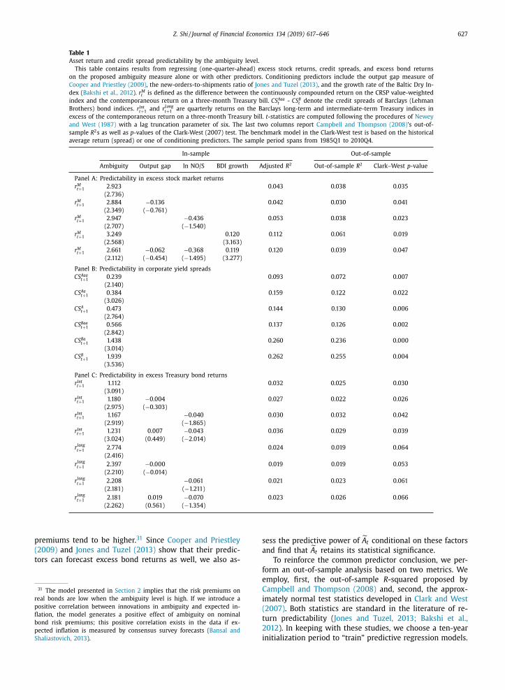
Z. Shi / Journal of Financial Economics 134 (2019) 617–646 627

Table 1

Asset return and credit spread predictability by the ambiguity level.

This table contains results from regressing (one-quarter-ahead) excess stock returns, credit spreads, and excess bond returns

on the proposed ambiguity measure alone or with other predictors. Conditioning predictors include the output gap measure of

Cooper and Priestley (2009) , the new-orders-to-shipments ratio of Jones and Tuzel (2013) , and the growth rate of the Baltic Dry In-

dex ( Bakshi et al., 2012 ). r M t is defined as the difference between the continuously compounded return on the CRSP value-weighted

index and the contemporaneous return on a three-month Treasury bill. CS Aaa t - CS B t denote the credit spreads of Barclays (Lehman

Brothers) bond indices. r Int t+1 and r Long

t+1 are quarterly returns on the Barclays long-term and intermediate-term Treasury indices in

excess of the contemporaneous return on a three-month Treasury bill. t -statistics are computed following the procedures of Newey

and West (1987) with a lag truncation parameter of six. The last two columns report Campbell and Thompson (2008) ’s out-of-

sample R 2 s as well as p -values of the Clark-West (2007) test. The benchmark model in the Clark-West test is based on the historical

average return (spread) or one of conditioning predictors. The sample period spans from 1985Q1 to 2010Q4.

In-sample Out-of-sample

Ambiguity Output gap ln NO/S BDI growth Adjusted R 2 Out-of-sample R 2 Clark–West p -value

Panel A: Predictability in excess stock market returns

r M t+1 2.923 0.043 0.038 0.035

(2.736)

r M t+1 2.884 −0.136 0.042 0.030 0.041

(2.349) ( −0.761)

r M t+1 2.947 −0.436 0.053 0.038 0.023

(2.707) ( −1.540)

r M t+1 3.249 0.120 0.112 0.061 0.019

(2.568) (3.163)

r M t+1 2.661 −0.062 −0.368 0.119 0.120 0.039 0.047

(2.112) ( −0.454) ( −1.495) (3.277)

Panel B: Predictability in corporate yield spreads

CS Aaa t+1 0.239 0.093 0.072 0.007

(2.140)

CS Aa t+1 0.384 0.159 0.122 0.022

(3.026)

CS A t+1 0.473 0.144 0.130 0.006

(2.764)

CS Baa t+1 0.566 0.137 0.126 0.002

(2.842)

CS Ba t+1 1.438 0.260 0.236 0.0 0 0

(3.014)

CS B t+1 1.939 0.262 0.255 0.004

(3.536)

Panel C: Predictability in excess Treasury bond returns

r Int t+1 1.112 0.032 0.025 0.030

(3.091)

r Int t+1 1.180 −0.004 0.027 0.022 0.026

(2.975) ( −0.303)

r Int t+1 1.167 −0.040 0.030 0.032 0.042

(2.919) ( −1.865)

r Int t+1 1.231 0.007 −0.043 0.036 0.029 0.039

(3.024) (0.449) ( −2.014)

r long t+1

2.774 0.024 0.019 0.064

(2.416)

r long t+1

2.397 −0.0 0 0 0.019 0.019 0.053

(2.210) ( −0.014)

r long t+1

2.208 −0.061 0.021 0.023 0.061

(2.181) ( −1.211)

r long t+1

2.181 0.019 −0.070 0.023 0.026 0.066

(2.262) (0.561) ( −1.354)

premiums tend to be higher. 31 Since Cooper and Priestley

(2009) and Jones and Tuzel (2013) show that their predic-

tors can forecast excess bond returns as well, we also as-

31 The model presented in Section 2 implies that the risk premiums on

real bonds are low when the ambiguity level is high. If we introduce a

positive correlation between innovations in ambiguity and expected in-

flation, the model generates a positive effect of ambiguity on nominal

bond risk premiums; this positive correlation exists in the data if ex-

pected inflation is measured by consensus survey forecasts ( Bansal and

Shaliastovich, 2013 ).

sess the predictive power of A t conditional on these factors

and find that ˜ A t retains its statistical significance.

To reinforce the common predictor conclusion, we per-

form an out-of-sample analysis based on two metrics. We

employ, first, the out-of-sample R -squared proposed by

Campbell and Thompson (2008) and, second, the approx-

imately normal test statistics developed in Clark and West

(2007) . Both statistics are standard in the literature of re-

turn predictability ( Jones and Tuzel, 2013; Bakshi et al.,

2012 ). In keeping with these studies, we choose a ten-year

initialization period to “train” predictive regression models.

628 Z. Shi / Journal of Financial Economics 134 (2019) 617–646

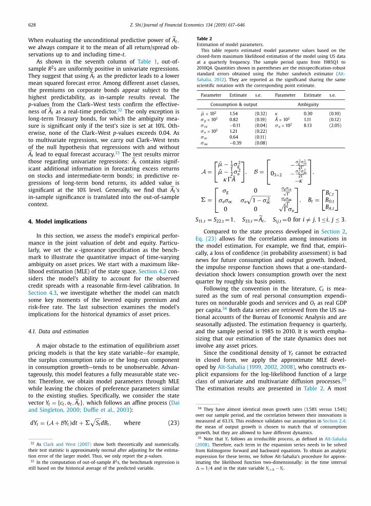
Table 2

Estimation of model parameters.

This table reports estimated model parameter values based on the

closed-form maximum likelihood estimation of the model using US data

at a quarterly frequency. The sample period spans from 1985Q1 to

2010Q4. Quantities shown in parentheses are the misspecification-robust

standard errors obtained using the Huber sandwich estimator ( Aït-

Sahalia, 2012 ). They are reported as the significand sharing the same

scientific notation with the corresponding point estimate.

Parameter Estimate s.e. Parameter Estimate s.e.

Consumption & output Ambiguity

μ × 10 2 1.54 (0.32) κ 0.30 (0.10)

σ g × 10 2 0.82 (0.19) A × 10 2 1.11 (0.12)

σ ca −0.11 (0.04) σ a × 10 2 8.13 (2.05)

σ o × 10 2 1.21 (0.22)

σ oc 0.64 (0.11)

σ oa −0.39 (0.08)

34 They have almost identical mean growth rates (1.58% versus 1.54%)

over our sample period, and the correlation between their innovations is

measured at 63.1%. This evidence validates our assumption in Section 2.4 :

When evaluating the unconditional predictive power of ˜ A t ,

we always compare it to the mean of all return/spread ob-

servations up to and including time- t .

As shown in the seventh column of Table 1 , out-of-

sample R 2 s are uniformly positive in univariate regressions.

They suggest that using A t as the predictor leads to a lower

mean squared forecast error. Among different asset classes,

the premiums on corporate bonds appear subject to the

highest predictability, as in-sample results reveal. The

p -values from the Clark–West tests confirm the effective-

ness of ˜ A t as a real-time predictor. 32 The only exception is

long-term Treasury bonds, for which the ambiguity mea-

sure is significant only if the test’s size is set at 10%. Oth-

erwise, none of the Clark–West p -values exceeds 0.04. As

to multivariate regressions, we carry out Clark–West tests

of the null hypothesis that regressions with and without ˜ A t lead to equal forecast accuracy. 33 The test results mirror

those regarding univariate regressions: ˜ A t contains signif-

icant additional information in forecasting excess returns

on stocks and intermediate-term bonds; in predictive re-

gressions of long-term bond returns, its added value is

significant at the 10% level. Generally, we find that ˜ A t ’s

in-sample significance is translated into the out-of-sample

context.

4. Model implications

In this section, we assess the model’s empirical perfor-

mance in the joint valuation of debt and equity. Particu-

larly, we set the κ-ignorance specification as the bench-

mark to illustrate the quantitative impact of time-varying

ambiguity on asset prices. We start with a maximum like-

lihood estimation (MLE) of the state space. Section 4.2 con-

siders the model’s ability to account for the observed

credit spreads with a reasonable firm-level calibration. In

Section 4.3 , we investigate whether the model can match

some key moments of the levered equity premium and

risk-free rate. The last subsection examines the model’s

implications for the historical dynamics of asset prices.

4.1. Data and estimation

A major obstacle to the estimation of equilibrium asset

pricing models is that the key state variable—for example,

the surplus consumption ratio or the long-run component

in consumption growth—tends to be unobservable. Advan-

tageously, this model features a fully measurable state vec-

tor. Therefore, we obtain model parameters through MLE

while leaving the choices of preference parameters similar

to the existing studies. Specifically, we consider the state

vector Y t = { c t , o t , A t } , which follows an affine process ( Dai

and Singleton, 20 0 0; Duffie et al., 2003 ):

dY t = (A + BY t ) dt + �√

S t dB t , where (23)

32 As Clark and West (2007) show both theoretically and numerically,

their test statistic is approximately normal after adjusting for the estima-

tion error of the larger model. Thus, we only report the p -values. 33 In the computation of out-of-sample R 2 s, the benchmark regression is

still based on the historical average of the predicted variable.

A =

[

μ − 1 2 σ 2

g

μ − 1 2 σ 2

o

κ�A

]

, B =

⎡ ⎣

− σ 2 g σ

2 ca

2�

0 3 ×2 − σ 2 o σ

2 oa

2�−κ

⎤ ⎦ ,

� =

⎡ ⎣

σg 0

σg σca √

�

σo σoc σo

√

1 − σ 2 oc

σo σoa √

�

0 0

√

�σa

⎤ ⎦ , B t =

[

B C,t

B O,t

B A,t

]

S 11 ,t = S 22 ,t = 1 , S 33 ,t =

A t , S i j,t = 0 for i � = j, 1 ≤ i, j ≤ 3 .

Compared to the state process developed in Section 2 ,

Eq. (23) allows for the correlation among innovations in

the model estimation. For example, we find that, empiri-

cally, a loss of confidence (in probability assessment) is bad

news for future consumption and output growth. Indeed,

the impulse response function shows that a one-standard-

deviation shock lowers consumption growth over the next

quarter by roughly six basis points.

Following the convention in the literature, C t is mea-

sured as the sum of real personal consumption expendi-

tures on nondurable goods and services and O t as real GDP

per capita. 34 Both data series are retrieved from the US na-

tional accounts of the Bureau of Economic Analysis and are

seasonally adjusted. The estimation frequency is quarterly,

and the sample period is 1985 to 2010. It is worth empha-

sizing that our estimation of the state dynamics does not

involve any asset prices.

Since the conditional density of Y t cannot be extracted

in closed form, we apply the approximate MLE devel-

oped by Aït-Sahalia (1999, 2002, 2008) , who constructs ex-

plicit expansions for the log-likelihood function of a large

class of univariate and multivariate diffusion processes. 35

The estimation results are presented in Table 2 . A most

the mean of output growth is chosen to match that of consumption

growth, but they are allowed to have different dynamics. 35 Note that Y t follows an irreducible process, as defined in Aït-Sahalia

(2008) . Therefore, each term in the expansion series needs to be solved

from Kolmogorov forward and backward equations. To obtain an analytic

expression for these terms, we follow Aït-Sahalia’s procedure for approx-

imating the likelihood function two-dimensionally: in the time interval

� = 1 / 4 and in the state variable Y t+� − Y t .

Z. Shi / Journal of Financial Economics 134 (2019) 617–646 629

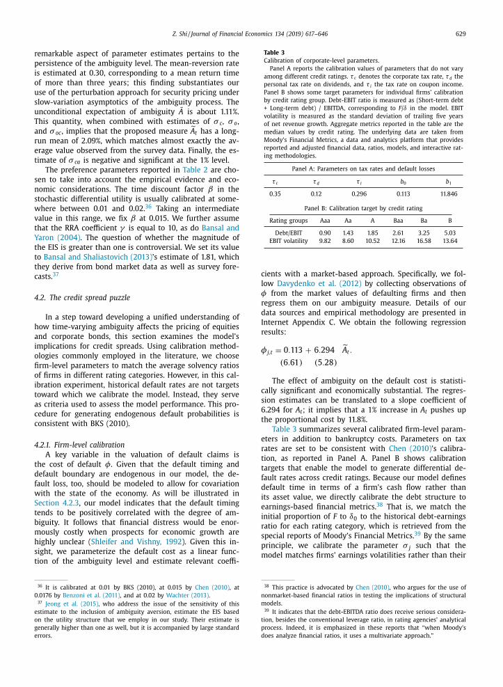
Table 3

Calibration of corporate-level parameters.

Panel A reports the calibration values of parameters that do not vary

among different credit ratings. τ c denotes the corporate tax rate, τ d the

personal tax rate on dividends, and τ i the tax rate on coupon income.

Panel B shows some target parameters for individual firms’ calibration

by credit rating group. Debt-EBIT ratio is measured as (Short-term debt

+ Long-term debt) / EBITDA, corresponding to F / δ in the model. EBIT

volatility is measured as the standard deviation of trailing five years

of net revenue growth. Aggregate metrics reported in the table are the

median values by credit rating. The underlying data are taken from

Moody’s Financial Metrics, a data and analytics platform that provides

reported and adjusted financial data, ratios, models, and interactive rat-

ing methodologies.

Panel A: Parameters on tax rates and default losses

τ c τ d τ i b 0 b 1

0.35 0.12 0.296 0.113 11.846

Panel B: Calibration target by credit rating

Rating groups Aaa Aa A Baa Ba B

Debt/EBIT 0.90 1.43 1.85 2.61 3.25 5.03

EBIT volatility 9.82 8.60 10.52 12.16 16.58 13.64

remarkable aspect of parameter estimates pertains to the

persistence of the ambiguity level. The mean-reversion rate

is estimated at 0.30, corresponding to a mean return time

of more than three years; this finding substantiates our

use of the perturbation approach for security pricing under

slow-variation asymptotics of the ambiguity process. The

unconditional expectation of ambiguity A is about 1.11%.

This quantity, when combined with estimates of σ c , σ o ,

and σ oc , implies that the proposed measure ˜ A t has a long-

run mean of 2.09%, which matches almost exactly the av-

erage value observed from the survey data. Finally, the es-

timate of σ ca is negative and significant at the 1% level.

The preference parameters reported in Table 2 are cho-

sen to take into account the empirical evidence and eco-

nomic considerations. The time discount factor β in the

stochastic differential utility is usually calibrated at some-

where between 0.01 and 0.02. 36 Taking an intermediate

value in this range, we fix β at 0.015. We further assume

that the RRA coefficient γ is equal to 10, as do Bansal and

Yaron (2004) . The question of whether the magnitude of

the EIS is greater than one is controversial. We set its value

to Bansal and Shaliastovich (2013) ’s estimate of 1.81, which

they derive from bond market data as well as survey fore-

casts. 37

4.2. The credit spread puzzle

In a step toward developing a unified understanding of

how time-varying ambiguity affects the pricing of equities

and corporate bonds, this section examines the model’s

implications for credit spreads. Using calibration method-

ologies commonly employed in the literature, we choose

firm-level parameters to match the average solvency ratios

of firms in different rating categories. However, in this cal-

ibration experiment, historical default rates are not targets

toward which we calibrate the model. Instead, they serve

as criteria used to assess the model performance. This pro-

cedure for generating endogenous default probabilities is

consistent with BKS (2010).

4.2.1. Firm-level calibration

A key variable in the valuation of default claims is

the cost of default φ. Given that the default timing and

default boundary are endogenous in our model, the de-

fault loss, too, should be modeled to allow for covariation

with the state of the economy. As will be illustrated in

Section 4.2.3 , our model indicates that the default timing

tends to be positively correlated with the degree of am-

biguity. It follows that financial distress would be enor-

mously costly when prospects for economic growth are

highly unclear ( Shleifer and Vishny, 1992 ). Given this in-

sight, we parameterize the default cost as a linear func-

tion of the ambiguity level and estimate relevant coeffi-

36 It is calibrated at 0.01 by BKS (2010), at 0.015 by Chen (2010) , at

0.0176 by Benzoni et al. (2011) , and at 0.02 by Wachter (2013) . 37 Jeong et al. (2015) , who address the issue of the sensitivity of this

estimate to the inclusion of ambiguity aversion, estimate the EIS based

on the utility structure that we employ in our study. Their estimate is

generally higher than one as well, but it is accompanied by large standard

errors.

cients with a market-based approach. Specifically, we fol-

low Davydenko et al. (2012) by collecting observations of

φ from the market values of defaulting firms and then

regress them on our ambiguity measure. Details of our

data sources and empirical methodology are presented in

Internet Appendix C. We obtain the following regression

results:

φ j,t = 0 . 113 + 6 . 294

˜ A t .

(6 . 61) (5 . 28)

The effect of ambiguity on the default cost is statisti-

cally significant and economically substantial. The regres-

sion estimates can be translated to a slope coefficient of

6.294 for A t ; it implies that a 1% increase in A t pushes up

the proportional cost by 11.8%.

Table 3 summarizes several calibrated firm-level param-

eters in addition to bankruptcy costs. Parameters on tax

rates are set to be consistent with Chen (2010) ’s calibra-

tion, as reported in Panel A. Panel B shows calibration

targets that enable the model to generate differential de-

fault rates across credit ratings. Because our model defines

default time in terms of a firm’s cash flow rather than

its asset value, we directly calibrate the debt structure to

earnings-based financial metrics. 38 That is, we match the

initial proportion of F to δ0 to the historical debt-earnings

ratio for each rating category, which is retrieved from the

special reports of Moody’s Financial Metrics. 39 By the same

principle, we calibrate the parameter σ j such that the

model matches firms’ earnings volatilities rather than their

38 This practice is advocated by Chen (2010) , who argues for the use of

nonmarket-based financial ratios in testing the implications of structural

models. 39 It indicates that the debt-EBITDA ratio does receive serious considera-

tion, besides the conventional leverage ratio, in rating agencies’ analytical

process. Indeed, it is emphasized in these reports that “when Moody’s

does analyze financial ratios, it uses a multivariate approach.”

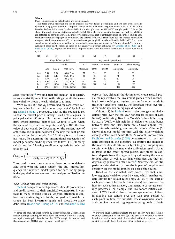
630 Z. Shi / Journal of Financial Economics 134 (2019) 617–646

Table 4

Model implications for default rates and credit spreads.

This table shows historical and model-implied ten-year default probabilities and ten-year credit spreads

by credit rating group. Column (2) reports average cumulative issuer-weighted default rates estimated from

Moody’s Default & Recovery Database (DRD) from Moody’s over the 1985–2015 sample period. Column (3)

shows the model-implied stationary default probabilities; the corresponding ten-year survival probabilities

are obtained by solving backward Kolmogorov equations on a grid of ambiguity levels. The model-implied 90%

confidence intervals displayed in Column (4) are derived from 50 0 0 simulations for the realized cumulative

ten-year default rates. Columns (5) reports median corporate yield spreads as listed in Table IA.E7. The corre-

sponding spread values corrected for the non-default component are shown in Columns (6) and (7); they are

calculated based on the fractional sizes of the liquidity component estimated by Longstaff et al. (2005) and

Chen et al. (2018) , respectively. Column (8) reports model-generated credit spreads for a special case with

A t ≡ A .

(1) (2) (3) (4) (5) (6) (7) (8) (9)

10-yr default prob(%) 10-yr credit spread(bp)

Model Total Credit Component Constant Time-varying

Data Mean 90% intvl. Observed LMN CCHM ambiguity ambiguity

Aaa 0.04 0.04 [0.00, 0.14] 77 39 33 8 32

Aa 0.45 0.42 [0.26, 0.75] 91 46 39 18 49

A 1.77 1.18 [0.87, 1.93] 117 66 67 53 78

Baa 3.66 4.24 [3.23, 6.39] 182 129 131 85 153

Ba 16.32 14.76 [13.41, 17.54] 298 247 241 164 225

B 37.64 40.13 [37.06, 45.96] 488 – – 312 407

C

asset volatilities. 40 We find that the median debt-EBITDA

ratios are strictly monotonic with ratings, while the earn-

ings volatility shows a weak relation to ratings.

With values of F and σ j determined for each credit rat-

ing, we solve for the total coupon payment C by follow-

ing Leland (1994a) ’s procedure. That is, the coupon is set

so that the market price of newly issued debt D equals its

principal value mF . As an illustration, consider Aaa-rated

firms whose historical debt-to-EBITDA ratio is 0.90. When

the value of corporate earnings starts at δ0 = 100 , the face

value of debt equals 90. Depending on the current level of

ambiguity, the coupon payment C making the debt priced

at par varies. For example, C = 5 . 61 if A 0 is at its histor-

ical mean. To determine the unconditional expectation of

model-generated credit spreads, we follow CCG (2009) by

calculating the following conditional spreads for selected

grids on A 0 :

¯ (A 0 ) =

(1

F − 1

( C (A 0 ) + mF ) PV

r+ m (A 0 )

).

Thus, credit spreads are computed based on a nondefault-

able bond with the same coupon rate and interest fre-

quency. The reported model spread for each rating group

is the population average over the steady-state distribution

of A t .

4.2.2. Default rates and credit spreads

Table 4 compares model-generated default probabilities

and credit spreads to their empirical counterparts. In con-

trast to many existing studies, wherein attention is con-

fined to investment-grade bonds, our goal is to match the

targets for both investment-grade and speculative-grade

debt. Both Huang and Huang (2012) and McQuade (2016)

40 Since the financial ratios covered by Moody’s Financial Metrics do not

include earnings volatility, the volatility of net revenue is used as a proxy.

An implicit assumption here is that the EBITDA margin is constant, and

thus revenue and EBITDA have the same growth rate.

observe that, although the documented credit spread puz-

zle mainly involves the investment grades, when reconcil-

ing it, we should guard against creating “another puzzle in

the other direction;” that is, the proposed model overpre-

dicts credit spreads on high-yield bonds.

Column (2) in Table 4 reports the average cumulative

default rates over the ten-year horizon for issuers of each

(initial) credit rating. Based on Moody’s Default & Recovery

Database (DRD), which includes all defaults on rated bonds

between 1970 and 2015, there are 22 (overlapping) ten-

year intervals matching our sample periods. Column (3)

shows that our model captures well the issuer-weighted

average default rates across these 22 cohorts. Noteworthily,

Feldhütter and Schaefer (2018) demonstrate that the stan-

dard approach in the literature—calibrating the model to

the realized default rates—is subject to great sampling un-

certainty, which may render the calibration results biased

in favor of the credit spread puzzle. Our study, in con-

trast, departs from this approach by calibrating the model

to debt ratios, as well as earnings volatilities, and thus en-

dogenously generates default rates. 41 Nevertheless, we still

perform a simulation to assess the impact of sampling un-

certainty on the model-implied ex post default rates.

Based on the estimated state process, we first simu-

late aggregate variables over 31 years, which matches our

data sample for default rates (1985–2015). At the start of

each year (except for the last nine years), we form one co-

hort for each rating category and generate corporate earn-

ings processes. For example, the Baa cohort initially con-

sists of 765 identical firms, the average number of firms

in Moody’s Baa cohorts over the 1985–2015 period. At

each point in time, we simulate 765 idiosyncratic shocks

and combine them with aggregate output growth to obtain

41 Our firm-level calibration targets, the debt-EBITDA ratio and earnings

volatility, correspond to the leverage ratio and asset volatility in value-

based structural models. With the standard calibration approach, asset

volatility is usually backed out from other calibration targets.

Z. Shi / Journal of Financial Economics 134 (2019) 617–646 631

firm-specific growth rates. As such, we can collect the re-

alized ten-year default frequency for each cohort and then

calculate the average rating-specific default rates in this

hypothetical economy. 42 Column (4) shows the 90% con-

fidence bands for the default rates derived from 50 0 0 sim-

ulations. These confidence intervals encompass the histor-

ical default rates for all rating groups, suggesting that the

modeled stationary default rates in Column (3) are recon-

cilable with the historical ones given the statistical uncer-

tainty associated with ex post default rates.

While matching the historical default rates indicates

how well the model quantifies the credit risk under the

physical measure, the model-generated credit spreads as-

sess the model’s performance under the risk-neutral mea-

sure. One important empirical consideration is what kind

of measure for history spread levels should be used for

comparison. The standard practice in the literature is to set

the firm’s leverage equal to the average leverage of firms in

a particular rating class and then compare model-implied

spreads with the (weighted) average actual spread over a

period. However, David (2008) and BKS (2010) are criti-

cal of this “averages-to-averages” comparison, as it is sub-

ject to convexity bias in credit spreads. 43 In this paper, we

adopt a “medians-to-medians” strategy: first, the model is

calibrated to the median financial ratios for a given rating

group; second, the model’s prediction is compared with

the median spread across all bonds in that rating category.

Internet Appendix shows that this approach is largely im-

mune to convexity bias.

The model’s implications for credit spreads are reported

in the right panel of Table 4 . It is well-known that non-

credit factors, such as illiquidity in the bond market, ac-

count for a sizable portion of yield spreads. Thus, in testing

the model’s predictions, we correct the target spreads for

the fractional liquidity components estimated by Longstaff

et al. (2005 , LMN hereinafter) and by Chen et al. (2018 ,

CCHM hereinafter). For example, the total yield for a typi-

cal Baa bond is about 182 basis points, as reported in Col-

umn (5) (also see Table IA.E7 in the Internet Appendix);

the estimate by LMN (2005) of Baa bonds’ liquidity frac-

tion is 29%. The credit component should account for

182 × 0.71 ≈ 129 basis points, as shown in Column (6). As

expected, the liquidity fraction of the total spread becomes

smaller as the rating quality of the bond decreases, while

42 Note that the default boundary is the same for these 765 firms be-

cause they start with the same initial debt-earnings ratio and are ex-

posed to the same degree of ambiguity throughout the simulated sam-

ple. Feldhütter and Schaefer (2018) find that the downward bias in real-

ized default rates is mainly attributable to the presence of systematic risk.

Systematic risk is present in our simulated economy as well: first, the

earnings process for individual firms contains a systematic component,

as specified in Eq. (15) ; second, the variation in the (fractional) default

boundary is driven by ambiguity shocks, which is common to all firms in

the economy. Therefore, untabulated results indicate that our simulated

ex post default rates share the same pattern as those of Feldhütter and

Schaefer (2018) ; that is, their distribution is skewed to the right and their

median is below the mean. 43 An early version of Feldhütter and Schaefer (2018) raises the same

point and attempted to quantify the convexity bias. Huang and Huang

(2012) and CCG (2009) find that if structure models are calibrated to the

historical default loss experience, the convexity effect is small and makes

the historical spreads even more of a puzzle.

the absolute magnitude of the liquidity component de-

creases with the credit rating.

We find that the model successfully captures the spread

level for both investment-grade bonds and high-yield

bonds. Our result indicates that we do not force the model

to match the historical spreads on high-quality bonds by

overstating the amount of compensation demanded for per

unit of default risk. In other words, this model improves

the pricing of corporate debt by producing a higher level

of uncertainty premium and proposing a better structure

for the market price of uncertainty. To underline the ef-

fect of time variation in ambiguity, we also tabulate the

credit spreads generated by time-invariant ambiguity. Col-

umn (7) in Table 4 indicates that the otherwise identical

κ-ignorance model substantially underperforms our bench-

mark model, especially for investment-grade bonds. In-

deed, the simplified model shows fairly limited improve-

ment over the baseline model where the agent is ambi-

guity neutral. This finding is consistent with CCG (2009),

who conclude that time-varying Sharpe ratios are essential

for explaining the credit spread puzzle.

4.2.3. Theoretical insights and empirical verification

However, time-varying asset Sharpe ratios alone do not

suffice to account for the high level of historical spreads—

a point illustrated by the baseline model of CCG (2009),

where the default boundary is constant. To explain the

credit spread puzzle, Sharpe ratios need to show a strong

correlation with the default time. In our model, it is ac-

complished by the optimal default boundary δ∗ that in-

creases with the level of ambiguity. This positive covari-

ation in turn drives up the risk-neutral default probability

far beyond its counterpart under the physical measure.

To demonstrate the effect of time-varying ambiguity on

the firm’s default decision, in Fig. 2 we plot δ∗ as a func-

tion of A t . We focus on a typical Baa-rated firm with the

current earnings level normalized to 100. The figure shows

that the default boundary is higher when the outlook for

economic growth is more unclear than usual. In other

words, management is more likely to exercise their default

option earlier in the presence of a high degree of ambi-

guity. While Knightian uncertainty has little impact on the

actual cash flows to the firm, it generates the comovement

between the default probability and market prices of un-

certainty.

Note that the ambiguity level also determines the as-

set valuation ratios. Numerically, its negative effect on the

price-earnings ratio L o dominates the positive effect on the

earnings-based default boundary. Thus, the asset value at

the time of default U

∗ is negatively related to A t , as in-

dicated by the dashed red line in Fig. 2 . 44 The direction

in which the default boundary moves actually constitutes

an important empirical basis used in model validation and

verification. For instance, Davydenko (2012) finds that the

value-based boundary is procyclical; this result supports

the prediction of Chen (2010) and BKS (2010). Following

44 This countermovement of default boundaries based on cash flows and

the asset value is also documented by Hackbarth et al. (2006) , Chen

(2010) , and BKS (2010).

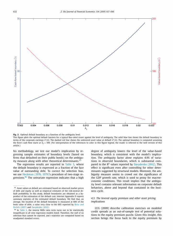
632 Z. Shi / Journal of Financial Economics 134 (2019) 617–646

0.002 0.004 0.006 0.008 0.01 0.012 0.014 0.016 0.018 0.02 0.02225

30

35

At

δC

ash-

flow

-bas

ed b

ound

ary

( *)

0.002 0.004 0.006 0.008 0.01 0.012 0.014 0.016 0.018 0.02 0.022160

180

200

Val

ue-b

ased

bou

ndar

y (U

* )

Fig. 2. Optimal default boundary as a function of the ambiguity level.

This figure plots the optimal default barriers for a typical Baa-rated issuer against the level of ambiguity. The solid blue line shows the default boundary in

terms of the corporate earnings δ∗( A ). The dashed red line shows the unlevered asset value at default U ∗( A ). The optimal boundary is computed assuming

the firm’s cash flow starts at δ0 = 100 . (For interpretation of the references to color in this figure legend, the reader is referred to the web version of this

article.)

his methodology, we test our model’s implication by re-

gressing sample estimates of boundary levels (based on

firms that defaulted on their public bonds) on the ambigu-

ity measure along with other theoretical determinants. 45

The regression results are reported in Table 5 , where

the default boundary is expressed as a fraction of the face

value of outstanding debt. To correct for selection bias,

we use Heckman (1976, 1979) ’s procedure of two-stage re-

gressions. 46 The univariate regression indicates that a high

45 Asset values at default are estimated based on observed market prices

of debt and equity as well as empirical estimates of the risk-neutral de-

fault probability. In this study, default boundaries are obtained as a by-

product of the estimation of the default cost. Internet Appendix D reports

summary statistics of the estimated default boundary. We find that, on

average, the location of the default boundary is measured at 68% of the

book value of debt, a value very close to the 66% reported by Reisz and

Perlich (2007) and Davydenko (2012) . 46 In Table 5 , the inverse Mills ratio term turns out to be statistically

insignificant in all nine regression models listed. Therefore, the null of no

selection bias cannot be rejected, and t -statistics are computed based on

unadjusted standard errors.

degree of ambiguity lowers the level of the value-based

boundary, which is consistent with the model’s implica-

tion. The ambiguity factor alone explains 4.9% of varia-

tions in observed boundaries, which is substantial com-

pared to the R 2 values reported by Davydenko (2012) . This

effect is significant even after controlling for other deter-

minants suggested by structural models. Moreover, the am-

biguity measure seems to crowd out the significance of

the GDP growth rate, which is used to proxy for macroe-

conomic conditions. This result implies that the ambigu-

ity level contains relevant information on corporate default

behaviors, above and beyond that contained in the busi-

ness cycle.

4.3. The levered equity premium and other asset pricing

implications

CCG (2009) describe calibration exercises on modeled

credit spreads as an out-of-sample test of potential solu-

tions to the equity premium puzzle. Given this insight, this

section brings the focus back to the equity premium by

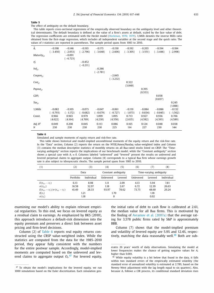
Z. Shi / Journal of Financial Economics 134 (2019) 617–646 633

Table 5

The effect of ambiguity on the default boundary.

This table reports cross-sectional regressions of the empirically observed boundary on the ambiguity level and other theoret-

ical determinants. The default boundary is defined as the value of a firm’s assets at default, scaled by the face value of debt.

The regression coefficients are estimated with the Heckit model ( Heckman, 1976; 1979 ). 1/ Mills denotes the inverse Mills ratio

obtained from the first-stage regression, which includes all independent variables at the second stage and the quick ratio. The

values of t -statistics are reported in parentheses. The sample period spans from 1983 to 2010.

˜ A t −0.198 −0.146 −0.193 −0.175 −0.150 −0.192 −0.203 −0.194 −0.184

( −3.450) ( −2.053) ( −2.796) ( −3.648) ( −2.606) ( −3.305) ( −3.551) ( −3.446) ( −2.998)

Maturity j,t −0.091

( −6.723)

rf t −0.452

( −0.211)

Vol j,t −0.286

( −2.781)

Coupon j,t −2.845

( −3.232)

Cost j,t 0.322

(3.040)

Payout j,t 0.395

(0.553)

GDP t 0.038

(0.837)

Tax j,t 0.245

(1.088)

1/ Mills −0.082 −0.105 −0.075 −0.047 −0.061 −0.119 −0.084 −0.086 −0.132

( −0.793) ( −1.172) ( −0.682) ( −0.679) ( −0.727) ( −1.073) ( −0.834) ( −0.845) ( −1.562)

Const. 0.966 0.965 0.979 1.099 1.095 0.713 0.927 0.936 0.706

(4.622) (4.164) (4.769) (4.230) (4.558) (2.635) (4.582) (4.393) (4.589)

Adj R 2 0.049 0.208 0.045 0.113 0.086 0.165 0.124 0.048 0.038

N 230 230 230 230 225 114 227 230 144

Table 6

Simulated and sample moments of equity return and risk-free rate.

This table shows historical and model-implied unconditional moments of the equity return and the risk-free rate.

In the “Data” section, Column (2) reports the return on the NYSE/Amex/Nasdaq value-weighted index and Column

(3) contains the median descriptive statistics of monthly returns on all Baa-rated stocks listed on CRSP. The “Time-

varying ambiguity” section reports the implications of our benchmark model, while the “Constant ambiguity” section

shows a special case with A t ≡ A . Columns labeled “unlevered” and “levered” present the results on unlevered and

levered perpetual claims to aggregate output. Column (8) corresponds to a typical Baa firm whose earnings growth

rate is also subject to idiosyncratic shocks. The sample period spans from 1985 to 2010.

(1) (2) (3) (4) (5) (6) (7) (8)

Data Constant ambiguity Time-varying ambiguity

Portfolio Individual Unlevered Levered Unlevered Levered Individual

E(r e,t − r t ) 6.13 8.98 1.11 2.09 4.13 5.94 7.81

σ ( r e,t ) 16.58 32.97 1.18 2.67 6.72 12.39 26.63

E(r e,t − r t ) /σ (r e,t − r t ) 41.49 28.33 93.97 78.62 73.75 48.60 29.24

E ( r t ) 1.21 1.70 1.18

σ ( r t ) 1.18 0 0.92

erates 26 years’ worth of daily observations. Simulating the model at

lower frequencies makes the chance of getting negative values for A t higher than 0.001.

48

examining our model’s ability to explain relevant empiri-

cal regularities. To this end, we focus on levered equity as

a residual claim to earnings. As emphasized by BKS (2010),

this approach introduces a default-risk dimension into the

equity premium and preserves a direct link between asset

pricing and firm-level decisions.

Column (2) of Table 6 reports real equity returns con-

structed using the CRSP value-weighted index. While the

statistics are computed from the data for the 1985–2010

period, they appear fully consistent with the numbers

for the entire postwar sample. Accordingly, model-implied

moments are computed based on the unlevered and lev-

ered claims to aggregate output O t . 47 For levered equity,

47 To obtain the model’s implications for the levered equity, we run

10 0 0 simulations based on the Euler discretization. Each simulation gen-

the initial ratio of debt to cash flow is calibrated at 2.61,

the median value for all Baa firms. This is motivated by

the finding of Avramov et al. (2007a) that the average rat-

ing for 3,578 public firms rated by S&P is approximately

BBB.

Column (7) shows that the model-implied premium

and volatility of levered equity are 5.9% and 12.4%, respec-

tively, matching the data reasonably well. 48 Both are sub-

While equity volatility is a bit below that found in the data, it falls

within two standard errors of the empirically estimated volatility (the

standard error of annualized volatility is estimated at 2.78%, based on the

Newey–West adjustment with the lag length equal to six quarters). Also,

because A t follows a CIR process, its conditional standard deviation rises

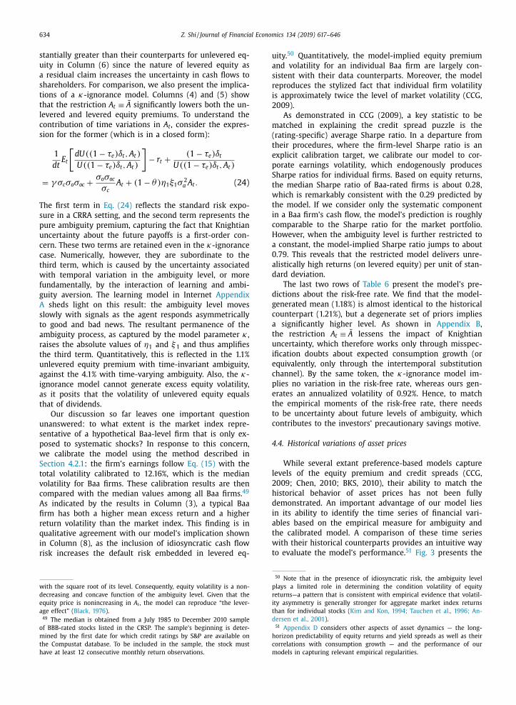
634 Z. Shi / Journal of Financial Economics 134 (2019) 617–646

stantially greater than their counterparts for unlevered eq-

uity in Column (6) since the nature of levered equity as

a residual claim increases the uncertainty in cash flows to

shareholders. For comparison, we also present the implica-

tions of a κ-ignorance model. Columns (4) and (5) show

that the restriction A t ≡ A significantly lowers both the un-

levered and levered equity premiums. To understand the

contribution of time variations in A t , consider the expres-

sion for the former (which is in a closed form):

1

dt E t

[dU((1 − τe ) δt , A t )

U((1 − τe ) δt , A t )

]− r t +

(1 − τe ) δt

U((1 − τe ) δt , A t )

= γ σc σo σoc +

σo σoc

σc A t + (1 − θ ) η1 ξ1 σ

2 a A t . (24)

The first term in Eq. (24) reflects the standard risk expo-

sure in a CRRA setting, and the second term represents the

pure ambiguity premium, capturing the fact that Knightian

uncertainty about the future payoffs is a first-order con-

cern. These two terms are retained even in the κ-ignorance

case. Numerically, however, they are subordinate to the

third term, which is caused by the uncertainty associated

with temporal variation in the ambiguity level, or more

fundamentally, by the interaction of learning and ambi-

guity aversion. The learning model in Internet Appendix

A sheds light on this result: the ambiguity level moves

slowly with signals as the agent responds asymmetrically

to good and bad news. The resultant permanence of the

ambiguity process, as captured by the model parameter κ ,

raises the absolute values of η1 and ξ 1 and thus amplifies

the third term. Quantitatively, this is reflected in the 1.1%

unlevered equity premium with time-invariant ambiguity,

against the 4.1% with time-varying ambiguity. Also, the κ-

ignorance model cannot generate excess equity volatility,

as it posits that the volatility of unlevered equity equals

that of dividends.

Our discussion so far leaves one important question

unanswered: to what extent is the market index repre-

sentative of a hypothetical Baa-level firm that is only ex-

posed to systematic shocks? In response to this concern,

we calibrate the model using the method described in

Section 4.2.1 : the firm’s earnings follow Eq. (15) with the

total volatility calibrated to 12.16%, which is the median

volatility for Baa firms. These calibration results are then

compared with the median values among all Baa firms. 49

As indicated by the results in Column (3), a typical Baa

firm has both a higher mean excess return and a higher

return volatility than the market index. This finding is in

qualitative agreement with our model’s implication shown

in Column (8), as the inclusion of idiosyncratic cash flow

risk increases the default risk embedded in levered eq-

with the square root of its level. Consequently, equity volatility is a non-

decreasing and concave function of the ambiguity level. Given that the

equity price is nonincreasing in A t , the model can reproduce “the lever-

age effect” ( Black, 1976 ). 49 The median is obtained from a July 1985 to December 2010 sample

of BBB-rated stocks listed in the CRSP. The sample’s beginning is deter-

mined by the first date for which credit ratings by S&P are available on

the Compustat database. To be included in the sample, the stock must

have at least 12 consecutive monthly return observations.

uity. 50 Quantitatively, the model-implied equity premium

and volatility for an individual Baa firm are largely con-

sistent with their data counterparts. Moreover, the model

reproduces the stylized fact that individual firm volatility

is approximately twice the level of market volatility (CCG,

2009).

As demonstrated in CCG (2009), a key statistic to be

matched in explaining the credit spread puzzle is the

(rating-specific) average Sharpe ratio. In a departure from

their procedures, where the firm-level Sharpe ratio is an

explicit calibration target, we calibrate our model to cor-

porate earnings volatility, which endogenously produces

Sharpe ratios for individual firms. Based on equity returns,

the median Sharpe ratio of Baa-rated firms is about 0.28,

which is remarkably consistent with the 0.29 predicted by

the model. If we consider only the systematic component

in a Baa firm’s cash flow, the model’s prediction is roughly

comparable to the Sharpe ratio for the market portfolio.

However, when the ambiguity level is further restricted to

a constant, the model-implied Sharpe ratio jumps to about

0.79. This reveals that the restricted model delivers unre-

alistically high returns (on levered equity) per unit of stan-

dard deviation.

The last two rows of Table 6 present the model’s pre-

dictions about the risk-free rate. We find that the model-

generated mean (1.18%) is almost identical to the historical

counterpart (1.21%), but a degenerate set of priors implies

a significantly higher level. As shown in Appendix B ,

the restriction A t ≡ A lessens the impact of Knightian

uncertainty, which therefore works only through misspec-

ification doubts about expected consumption growth (or

equivalently, only through the intertemporal substitution

channel). By the same token, the κ-ignorance model im-

plies no variation in the risk-free rate, whereas ours gen-

erates an annualized volatility of 0.92%. Hence, to match

the empirical moments of the risk-free rate, there needs

to be uncertainty about future levels of ambiguity, which

contributes to the investors’ precautionary savings motive.

4.4. Historical variations of asset prices

While several extant preference-based models capture

levels of the equity premium and credit spreads (CCG,

2009; Chen, 2010; BKS, 2010), their ability to match the

historical behavior of asset prices has not been fully

demonstrated. An important advantage of our model lies

in its ability to identify the time series of financial vari-

ables based on the empirical measure for ambiguity and

the calibrated model. A comparison of these time series

with their historical counterparts provides an intuitive way

to evaluate the model’s performance. 51 Fig. 3 presents the

50 Note that in the presence of idiosyncratic risk, the ambiguity level

plays a limited role in determining the condition volatility of equity

returns—a pattern that is consistent with empirical evidence that volatil-

ity asymmetry is generally stronger for aggregate market index returns

than for individual stocks ( Kim and Kon, 1994; Tauchen et al., 1996; An-

dersen et al., 2001 ). 51 Appendix D considers other aspects of asset dynamics — the long-

horizon predictability of equity returns and yield spreads as well as their

correlations with consumption growth — and the performance of our

models in capturing relevant empirical regularities.

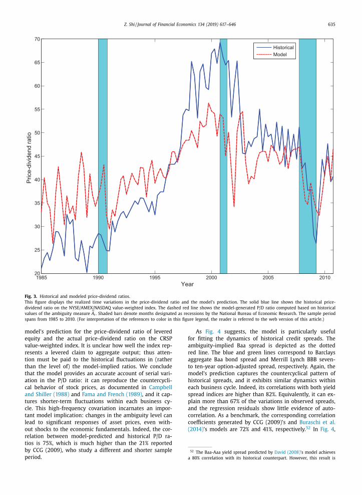
Z. Shi / Journal of Financial Economics 134 (2019) 617–646 635

1985 1990 1995 2000 2005 201020

25

30

35

40

45

50

55

60

65

70

Year

Pric

e-di

vide

nd ra

tio

HistoricalModel

Fig. 3. Historical and modeled price-dividend ratios.

This figure displays the realized time variations in the price-dividend ratio and the model’s prediction. The solid blue line shows the historical price-

dividend ratio on the NYSE/AMEX/NASDAQ value-weighted index. The dashed red line shows the model-generated P/D ratio computed based on historical

values of the ambiguity measure A t . Shaded bars denote months designated as recessions by the National Bureau of Economic Research. The sample period

spans from 1985 to 2010. (For interpretation of the references to color in this figure legend, the reader is referred to the web version of this article.)

52 The Baa-Aaa yield spread predicted by David (2008) ’s model achieves

a 80% correlation with its historical counterpart. However, this result is

model’s prediction for the price-dividend ratio of levered

equity and the actual price-dividend ratio on the CRSP

value-weighted index. It is unclear how well the index rep-

resents a levered claim to aggregate output; thus atten-

tion must be paid to the historical fluctuations in (rather

than the level of) the model-implied ratios. We conclude

that the model provides an accurate account of serial vari-

ation in the P/D ratio: it can reproduce the countercycli-

cal behavior of stock prices, as documented in Campbell

and Shiller (1988) and Fama and French (1989) , and it cap-

tures shorter-term fluctuations within each business cy-

cle. This high-frequency covariation incarnates an impor-

tant model implication: changes in the ambiguity level can

lead to significant responses of asset prices, even with-

out shocks to the economic fundamentals. Indeed, the cor-

relation between model-predicted and historical P/D ra-

tios is 75%, which is much higher than the 21% reported

by CCG (2009), who study a different and shorter sample

period.

As Fig. 4 suggests, the model is particularly useful

for fitting the dynamics of historical credit spreads. The

ambiguity-implied Baa spread is depicted as the dotted

red line. The blue and green lines correspond to Barclays

aggregate Baa bond spread and Merrill Lynch BBB seven-

to ten-year option-adjusted spread, respectively. Again, the

model’s prediction captures the countercyclical pattern of

historical spreads, and it exhibits similar dynamics within

each business cycle. Indeed, its correlations with both yield

spread indices are higher than 82%. Equivalently, it can ex-

plain more than 67% of the variations in observed spreads,

and the regression residuals show little evidence of auto-

correlation. As a benchmark, the corresponding correlation

coefficients generated by CCG (2009)’s and Buraschi et al.

(2014) ’s models are 72% and 41%, respectively. 52 In Fig. 4 ,

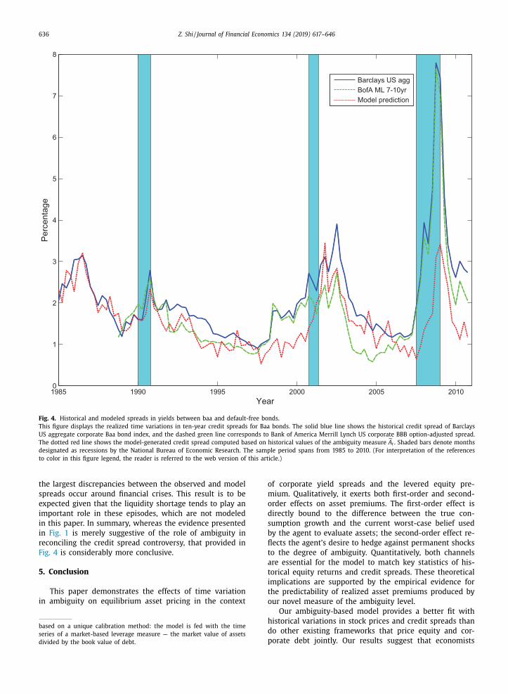
636 Z. Shi / Journal of Financial Economics 134 (2019) 617–646

1985 1990 1995 2000 2005 20100

1

2

3

4

5

6

7

8

Year

Per

cent

age

Barclays US aggBofA ML 7-10yrModel prediction

Fig. 4. Historical and modeled spreads in yields between baa and default-free bonds.

This figure displays the realized time variations in ten-year credit spreads for Baa bonds. The solid blue line shows the historical credit spread of Barclays

US aggregate corporate Baa bond index, and the dashed green line corresponds to Bank of America Merrill Lynch US corporate BBB option-adjusted spread.

The dotted red line shows the model-generated credit spread computed based on historical values of the ambiguity measure A t . Shaded bars denote months

designated as recessions by the National Bureau of Economic Research. The sample period spans from 1985 to 2010. (For interpretation of the references

to color in this figure legend, the reader is referred to the web version of this article.)

the largest discrepancies between the observed and model

spreads occur around financial crises. This result is to be

expected given that the liquidity shortage tends to play an

important role in these episodes, which are not modeled

in this paper. In summary, whereas the evidence presented

in Fig. 1 is merely suggestive of the role of ambiguity in

reconciling the credit spread controversy, that provided in

Fig. 4 is considerably more conclusive.

5. Conclusion

This paper demonstrates the effects of time variation

in ambiguity on equilibrium asset pricing in the context

based on a unique calibration method: the model is fed with the time

series of a market-based leverage measure — the market value of assets

divided by the book value of debt.

of corporate yield spreads and the levered equity pre-

mium. Qualitatively, it exerts both first-order and second-

order effects on asset premiums. The first-order effect is

directly bound to the difference between the true con-

sumption growth and the current worst-case belief used

by the agent to evaluate assets; the second-order effect re-

flects the agent’s desire to hedge against permanent shocks

to the degree of ambiguity. Quantitatively, both channels

are essential for the model to match key statistics of his-

torical equity returns and credit spreads. These theoretical

implications are supported by the empirical evidence for

the predictability of realized asset premiums produced by

our novel measure of the ambiguity level.

Our ambiguity-based model provides a better fit with

historical variations in stock prices and credit spreads than

do other existing frameworks that price equity and cor-

porate debt jointly. Our results suggest that economists

Z. Shi / Journal of Financial Economics 134 (2019) 617–646 637

should look beyond the business cycle when characteriz-

ing the dynamics of asset prices. In the framework of Chen

(2010) and BKS (2010), the model’s fit to the historical

yield spreads is sacrificed through a discretization of ex-

pected consumption growth and consumption volatility. In

this manner, they are able to deliver closed-form solutions

to equity and debt prices with dynamic capital structure.

Given this insight, an extension of our model to allow for

endogenous capital structure presents an interesting topic

for future research. Agency costs and transaction (debt re-

tirement and reissuance) costs, as considered by Leland

(1998) and Strebulaev (2007) , can be incorporated into the

extended model as well.

Another interesting direction for future research is to

consider the implications of our model for derivative pric-

ing. For instance, one can introduce secondary market

search frictions ( He and Milbradt, 2014 ) and evaluate

the model’s performance in fitting bond-CDS spreads (the

non-default components of corporate yield spreads). Also,

our model can be extended to shed light on stylized

facts about option-implied volatility, that is, the “volatility

smirk” and the variance premium, as studied by Drechsler

(2013) . 53

Appendix A. More properties of the proposed

ambiguity measure

This appendix supplements Section 3.1 with more de-

tails on the properties of ˜ A t . The first two sections

draw a comparison of ˜ A t with other empirical measures

based on the dispersion of survey forecasts. Specifically,

Section A.1 covers alternative ambiguity measures, and

Section A.2 considers empirical proxies proposed for het-

erogeneous beliefs models. The relations of all these mea-

sures (including ˜ A t ) with macroeconomic volatility are ex-

amined in Section A.3 .

A.1. Alternative measures of ambiguity

In this section, we place the proposed empirical mea-

sure in the context of relevant literature by comparing

it with alternative ambiguity measures used in existing

studies. AGJ is arguably the first to test the link between

time-varying ambiguity and asset pricing by constructing

an index of Knightian uncertainty. The key “ambiguous”

variable in their model is the expected real return on the

market portfolio in excess of the risk-free rate. To con-

struct a relevant ambiguity measure, they collect from the

SPF panelists’ predictions on several economic variables,

including corporate profits after taxes, GDP deflator, and

nominal T-bill rates. With these variables, they impute

53 Drechsler (2013) specifies an exogenous dividend process and treats

equity as an unlevered claim to the dividend. Therefore, his model could

be calibrated less aggressively than he does to capture qualitative features

of the equity premium and variance premium. Also, if we embed a struc-

tural credit model into his framework with the firm-level parameters the

same as in our model, we find that his calibration tends to overpredict

corporate default rates and credit spreads when the default barrier is set

endogenously. When the default boundary is set as constant (at 68% of

the book value of debt), the model-generated yield spreads become in-

sufficient to match the empirical credit spreads.

each participant’s forecast of real market return based on

Gordon’s formula and then proxy the level of ambiguity

by a weighted variance of forecasts. By the same spirit,

Drechsler (2013) proposes a measure based on the cross-

sectional standard deviation in SPF forecasts of real GDP

growth, which is used to provide empirical support for a

link between ambiguity and the variance premium.

It is noteworthy that both measures are conceptually

consistent with the way they construct the set of alter-

native beliefs. Specifically, they set a upper bound for the

(growth rate of) relative entropy, 54 which, in this paper’s

setting, is equivalent to a upper bound for the norm of

the density generator ( ϑt ). This approach to restricting the

amount of ambiguity is adopted in Hansen and Sargent

(2008) ’s robust control framework. With multiple-priors

preferences, in contrast, the belief set is restricted by a

rectangular set of density generators. This rectangularity

inspires our use of cross-sectional range, rather than vari-

ance (standard deviation), as the ambiguity measure.

The empirical measure used in Ilut and Schneider

(2014) is another example of using the interdecile range

of survey forecasts to infer the dynamics of ambiguity

in multiple-priors models. In an early version ( Ilut and

Schneider, 2011 ), their measure is based on the difference

between the 75th percentile and the 25th percentile in

each cross-section of forecasts. The resulting interquartile

range is essentially the Federal Reserve Bank of Philadel-

phia’s definition of “forecast dispersion” and is included in

its SPF database. In Table A.1 , we make a comparison of

our ambiguity measure with the three alternative ones as

aforementioned.

Panel A provides a description for each empirical mea-

sure and particularly highlights their forecasting perfor-

mance. Because of the space limitations, only the p -values

obtained from univariate regressions of equity returns are

reported. We focus on stocks here, as almost all asset pric-

ing models carry implications for the equity premium but

not necessarily for other asset classes. We find that the

AGJ measure is the only one (besides our measure ˜ A t )

with significant forecasting power. The correlation between

their measure and ours is not remarkable, at approximately

25%, which is not surprising given that they are meant to

capture the agent’s confidence about different economic

quantities. However, they do share some notable similar-

ities in the way they are constructed. In particular, both

their weighted variance and our interdecile range allow for

the possibility of minimizing the impact of extreme fore-

casts. 55 As discussed in Epstein and Schneider (2003) , the

difference between the multiple-priors and robust control

models is a matter of alternative restrictions on the belief

sets and on updating rules and which type of restriction to

be imposed in ambiguity modeling “will typically depend

on the application.” Our result suggests that, at least in

54 Relative entropy is the Kullback–Leibler distance between an alterna-

tive probability measure and the reference measure. 55 When computing the weighted variance of forecasts, AGJ assign the

weight to each forecast based on a discretized beta distribution. They

force both shape parameters to be equal and greater than one such that

the weight is symmetric and heavily penalizes observations lying on the

left and right tails.

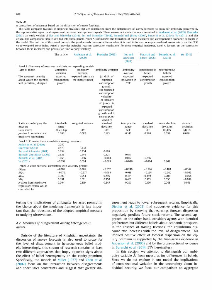
638 Z. Shi / Journal of Financial Economics 134 (2019) 617–646

Table A1

A comparison of measures based on the dispersion of survey forecasts.

This table compares features of empirical measures that are constructed from the distributions of survey forecasts to proxy for ambiguity perceived by

the representative agent or disagreement between heterogeneous agents. These measures include the ones examined in Anderson et al. (2009) , Drechsler

(2013) , an early version of Ilut and Schneider (2014) , Ilut and Schneider (2011) , Buraschi and Jiltsov (2006) , Buraschi et al. (2014) , Yu (2011) , and this

article. The comparison table is divided into three panels. Panel A summarizes the formation of these measures and corresponding economic concepts in

the model. The last row of this panel presents the p -value each measure achieves when it is used to forecast one-quarter-ahead excess return on the CRSP

value-weighted stock index. Panel B provides pairwise Pearson correlation coefficients for these empirical measures. Panel C focuses on the correlation

between these measures and proxies for time-varying volatility.

This article Anderson et al.

(2009)

Drechsler (2013) Ilut and

Schneider

(2011)

Buraschi and

Jiltsov (2006)

Buraschi et al.

(2014)

Yu (2011)

Panel A: Summary of measures and their corresponding models

Type of model ambiguity

aversion

ambiguity

aversion

ambiguity aversion ambiguity

aversion

heterogeneous

beliefs

heterogeneous

beliefs

The economic quantity

about which the agent(s)

feel uncertain / disagree

expected

consumption

growth

expected return on

the market index

(a) drift of

expected

consumption

growth;

(b) expected

consumption

volatility;

(c) intensity

of jumps in

expected

consumption

growth and in

consumption

volatility

expected

innovation in

TFP

expected

consumption

growth

expected

consumption

growth

Statistics underlying the

measure

interdecile

range

weighted variance standard

deviation

interquartile

range

standard

deviation

mean absolute

deviation

standard

deviation

Data source Blue Chip SPF SPF SPF SPF I/B/E/S I/B/E/S

p -value from univariate

predictive regressions

0.003 0.082 0.183 0.143 0.280 0.037 0.096

Panel B: Cross-sectional correlation among measures

Anderson et al. (2009) 0.250

Drechsler (2013) 0.479 0.192

Ilut and Schneider (2011) 0.634 0.234 0.665

Buraschi and Jiltsov (2006) 0.625 0.144 0.521 0.671

Buraschi et al. (2014) 0.068 0.166 −0.004 0.032 0.216

Yu (2011) −0.038 0.024 −0.063 −0.046 −0.004 0.261

Panel C: Cross-sectional correlation with volatility proxies

EV GDP,t −0.105 0.005 −0.057 −0.240 −0.274 −0.163 −0.147

RV IP,t −0.170 −0.217 −0.068 0.018 −0.198 −0.240 −0.085

RV M,t 0.302 0.053 0.296 0.354 0.459 0.205 −0.068

VIX t 0.391 0.021 0.350 0.401 0.413 0.050 −0.099

p -value from predictive

regressions when VIX t is

controlled for

0.004 0.119 0.245 0.243 0.156 0.048 0.059

testing the implications of ambiguity for asset premiums,

the choice about the modeling framework is less impor-

tant than the robustness of the adopted empirical measure

to outlying observations.

A.2. Measures of disagreement among heterogeneous

agents

Outside of the literature of Knightian uncertainty, the

dispersion of survey forecasts is also used to proxy for

the level of disagreement in heterogeneous belief mod-

els. Interestingly, this stream of research contains at least

two different approaches that imply opposite signs about

the effect of belief heterogeneity on the equity premium.

Specifically, the models of Miller (1977) and Chen et al.

(2002) focus on the interaction between disagreements

and short sales constraints and suggest that greater dis-

agreement leads to lower subsequent returns. Empirically,

Diether et al. (2002) find supportive evidence for this

proposition by showing that earnings forecast dispersion

negatively predicts future stock returns. The second ap-

proach, on the other hand, considers agents with identical

preferences but different beliefs about economic prospects.

In the absence of trading frictions, the equilibrium dis-

count rate increases with the level of disagreement. This

implied positive effect of forecast dispersion on the eq-

uity premium is supported by the time-series evidence in

Anderson et al. (2005) and by the cross-sectional evidence

in Buraschi et al. (2014 , BTV hereinafter).

In this section, we attempt to distinguish our ambi-

guity variable ˜ A t from measures for differences in beliefs.

Since we do not explore in our model the implications

of cross-sectional variation in the uncertainty about in-

dividual security, we focus our comparison on aggregate

Z. Shi / Journal of Financial Economics 134 (2019) 617–646 639

disagreement indices. 56 Regarding the disagreement-with-

short-sales-constraint approach, we consider Yu (2011) ’s

measure, which can be regarded as an aggregation of

Diether et al. (2002) ’s or AGJ (2005) ’s individual-level mea-

sures and a proxy for the disagreement about aggregate

corporate earnings. Among studies with the second ap-

proach, we select the measures constructed by Buraschi

and Jiltsov (2006) and BTV (2014) . The former measure

is the first principal component of differences in beliefs

about six economic variables, where the difference in be-

liefs is defined as the cross-sectional standard deviation of

SPF forecasts. The latter is similar to Yu (2011) ’s measure in

the sense that it is constructed bottom-up by aggregating

disagreements regarding the earnings of individual firms.

The biggest difference between them arises from the un-

derlying statistics: Yu (2011) uses the standard deviation

of analyst forecasts, whereas BTV (2014) adopt the mean

absolute difference (the average of absolute differences be-

tween each pair of earnings forecasts).

Panel A of Table A.1 indicates that the measure of

BTV (2014) is highly significant in forecasting one-quarter-

ahead market returns, and Yu (2011) ’s measure exhibits

statistical significance at the 10% level. Unreported results

show that both slope coefficients are negative, which is

not surprising given that both measures are constructed

bottom-up using the same dataset (I/B/E/S). While this is

consistent with Yu (2011) ’s interpretation, it is opposite to

the implications from BTV (2014) ’s model. 57 In contrast,

the sign of the regression coefficient is positive for the

Buraschi–Jiltsov measure, even though the null of no pre-

dictability cannot be rejected at any conventional signifi-

cance level.

While both our ambiguity measure and aforemen-

tioned disagreement measures are extracted from fore-

cast dispersion, they have distinct properties, the most

noticeable being the underlying statistics and predictive

ability. We find that the range-based measures seem to

be exclusively used in studies with multiple-priors util-

ity, for the reason explained in the last subsection. One

may argue that standard-deviation-based measures for

disagreements—which are particularly relevant when we

assume that each agent corresponds exactly to one partic-

ipating forecaster (AGJ, 2005) —could also be used to proxy

for Knightian uncertainty in multiplier models (AGJ, 2009;

Drechsler, 2013) and thus are conceptually related to our

measure ˜ A t . However, those measures show either a low

(or even negative) empirical correlation with

˜ A t or limited

explanatory power for asset premiums.

Both findings merit further discussion. First, the neg-

ative correlation coefficient between

˜ A t and Yu (2011) ’s

measure, as displayed in Panel B, reinforces his support-

ive evidence for the Miller (1977) conjecture (about the

negative effect of disagreement on expected stock returns).

56 In other words, we do not consider disagreements about the earnings

of individual stocks ( Diether et al., 2002 ) nor disagreement factors con-

structed as the returns from longing high-dispersion stocks and shorting

low-dispersion stocks (AGJ, 2005) . 57 BTV (2014) find that their measure represents a positively priced risk

in the cross section of stock returns, but they do not test the return pre-

dictability with this measure.

Second, at first glance the insignificance of the Buraschi–

Jiltsov measure in predicting equity returns is somewhat

inconsistent with their model, which implies that differ-

ences in beliefs should be a significant determinant of the

equity premium. If we interpret this result from a differ-

ence perspective, it nevertheless may actually reflect a key

difference between two classes of models. In the models of

Buraschi and Jiltsov (2006) and BTV (2014) , it is the inter-

action between the degree of belief heterogeneity and the

consumption share of the optimist, instead of either com-

ponent alone, that drives the variation in equity premium.

This interaction is absent in models with a representative

ambiguity-averse agent. Therefore, the missing-variable is-

sue could potentially explain why their measures are in-

significant or have the wrong sign in univariate predictive

regressions.

A.3. Relation with time-varying volatility

Another possible interpretation of forecast dispersion

that deserves discussion is that it captures macroeco-

nomic volatility. Theoretically, Bansal and Yaron (2004) and

Bansal et al. (2014 , BKSY hereinafter) posit that an increase

in volatility is associated with a rise in discount rates, a

prediction similar to our model’s implication for ambigu-

ity. Hence, it is important to draw a distinction between

measures of time-varying ambiguity and those of time-

varying volatility. In this section, we perform a compar-

ative analysis of these empirical measures by considering

both macroeconomic and return-based proxies for volatil-

ity as used in BKSY: the realized variances of industrial

production growth rates and market returns.

For robustness, we examine as well the difference of ˜ A t

from Bansal and Shaliastovich (2013) ’s measure of the ex-

pected variance of consumption growth. That is, they es-

timate innovations in the SPF consensus (mean) forecast

of real GDP growth and then regress annual sum squares

of future innovations on the current explanatory variables

to obtain the time series of expected (fitted) consump-

tion variance. Finally, given that both the BKSY ex post

measure and the Bansal–Shaliastovich ex ante measure are

about volatility under the physical measure, we also in-

clude in our comparison the option-implied variance (VIX)

as a proxy for the Q -measure volatility.

Panel C of Table A.1 shows that our ambiguity measure

does not have a particularly high correlation with any of

the four volatility proxies. The correlation coefficients with

respect to macroeconomic-based volatility proxies are even

negative. 58 More importantly, ˜ A t preserves the same level

of statistical significance in predicting equity returns when

we control for VIX, the volatility proxy with the greatest

predictive power. 59 It implies that ˜ A t contains information

58 Results regarding return-based volatility proxies should be down-

weighted, in the sense that based on the model presented in Section 2 ,

the volatility of levered equity is a nonlinear function of the ambigu-

ity level. Therefore, even if consumption growth exhibits time-varying

volatility, it is intertwined with time-varying ambiguity in the determi-

nation of equity volatility in equilibrium. 59 The R 2 from univariate regression of excess stock returns on VIX is

about 0.023, and the t -statistic for VIX is 0.927.

640 Z. Shi / Journal of Financial Economics 134 (2019) 617–646

60 Note that allowing for serial covariations between c t and A t results

in another 0.05% decrease in ϱ1 , which partially accounts for the gap be-

tween risk-free rates generated by the models with and without time-

varying ambiguity. This cross-shock effect is reflected by the last term in

Eq. (B.2b) .

regarding risk premiums independent of stochastic volatil-

ity.

The results for other measures (based on forecast dis-

persion) as discussed above are also reported for complete-

ness. We find that among these six measures, the one con-

structed by Buraschi and Jiltsov (2006) displays the high-

est correlation with time-varying volatility. For those with

significant forecasting power for equity returns, their sig-

nificance is generally unaffected by the inclusion of VIX.

This finding suggests that volatility drives time variations

in the asset premium through a risk channel that is dis-

tinct from those for time-varying ambiguity and heteroge-

neous beliefs.

Appendix B. Equilibrium prices and affine

approximation

Given the value function of the representative agent as

defined in Eq. (6) , to make J(C t , A t ) +

∫ t 0 f (C s , J(C s , A s )) ds

a martingale under the most pessimistic probability mea-

sure, we have

D

C,A J + f (C, J) − θ ∗(A ) J C Cσc = 0 .

Conjecture that J has the functional form in Eq. (12) .

Substituting it into the differential equation above, we ob-

tain

(1 − γ ) (μc − A − 1

2

γ σ 2 c +

(L A L

θσa − 1

2

γ σc σca

)σc σca A

)+

D

A L θ

L θ+

θ

L − βθ = 0 , γ , ψ � = 1 . (B.1)

Eq. (11) in Proposition 1 is a special case with the correla-

tion parameter σ ca equal to zero.

To solve the model, we employ Collin-Dufresne and

Goldstein (2005) ’s log-linear approximation that essen-

tially minimizes the expected squared approximation error.

Specifically, we seek an exponential affine expression for

the price-consumption ratio as presented in Eq. (13) such

that the left-hand side of Eq. (B.1) is linear in A t except for

the θ / L term. In that case, the parameters η0 and η1 can be

obtained by solving the following optimization problem:

min

η0 ,η1

E [(n 0 + n 1 A t − θe −η0 −η1 A t ) 2

],

where

−n 0 = (1 − γ ) (μc − 1

2

γ σ 2 c

)+ θ (η1 κ A − β) ,

−n 1 = (1 − γ ) ((

η1 θσa − 1

2

γ σc σca

)σc σca − 1

)− θ

(η1 κ − 1

2

θη2 1 σ

2 a

).

Fig. B.1 makes a comparison of this approximate price-

consumption ratio with the one numerically solved from

Eq. (11) . These two solutions turn out to be fairly close

to each other. Indeed, when the ambiguity level is around

its long-run mean, they are almost indistinguishable from

each other. This result demonstrates the accuracy of the

exponential affine approximation.

With first-order conditions for the optimal consumption

choice under ambiguity, Chen and Epstein (2002) drive the

following SDF:

M t = e ∫ t

0 f J (C s ,J s ) ds f C (C t , J t ) Z θ∗t ,

where Z θ∗ is the Radon–Nikodym derivative corresponding

to the worse-case prior. The multiple-priors preference is

reflected in the presence of Z θ∗: if P 0 is the only belief in

the prior set P, it degenerates to one, and the SDF be-

comes the standard one in Duffie and Epstein (1992) and

Duffie and Skiadas (1994) .

To prove Proposition 2 , we apply Itô’s lemma to the

pricing kernel. It follows that

r t = −E

(dM t

M t dt

)= γ

[ μc − A − 1

2

(1 + γ )(1 + σ 2 ca A ) σ 2

c

+

L A L

(θ − 1) σc σa σca

] − D

A L θ−1

L θ−1 − θ − 1

L + βθ.

Connecting it with Eq. (11) , we obtain the risk-free rate as

a linear function of the ambiguity level

r t = � 0 + � 1 A t ,

where

� 0 = μc /ψ + β − 1

2

γ (1 + 1 /ψ) σ 2 c , (B.2a)

� 1 = − 1 /ψ +

1

2 (θ − 1) η2

1 σ2 a

+

((θ − 1) η1 σa − 1

2 γ (1 + 1 /ψ) σc σca

)σc σca . (B.2b)

If consumption growth is a random walk independent

of innovations in the ambiguity level, the last term in

Eq. (B.2b) vanishes.

It follows that the dual role time-varying ambiguity

serves in equilibrium asset pricing is also reflected in its

impact on the risk-free rate. The first term on the right-

hand side of Eq. (B.2b) captures the effect of ambiguity

on intertemporal smoothing. Also persisting in the case of

constant ambiguity, it underlines the fact that ambiguity

about the distribution of future payoffs is a first-order con-

cern. However, the second term is absent in models with

either time-invariant ambiguity or constant relative risk

aversion ( θ = 1 ). The agent’s preference for early resolution

of uncertainty would lower the equilibrium interest rate

because she wants to divest from risky assets when the

future level of ambiguity becomes highly uncertain. There-

fore, both effects enhance the agent’s saving motive and

thus help to explain the risk-free rate puzzle.

As shown in Table 6 , the drift perturbation term in

Eq. (B.2b) decreases the mean of r t by merely A /ψ = 0 . 61% ,

which is not enough to account for the risk-free rate puz-

zle. Therefore, the second term (θ − 1) η2 1 σ

2 a / 2 , which is

missing in the constant-ambiguity case, is necessary to

capture the low mean of historical interest rates. It symbol-

izes the precautionary saving motive caused by unknown

future levels of ambiguity and leads to another 0.48% re-

duction in the unconditional expectation of r t . 60 Hence,

Z. Shi / Journal of Financial Economics 134 (2019) 617–646 641

Fig. B1. Approximate solution for the price-consumption ratio.

This figure shows the accuracy of our approximation of the price-consumption ratio L t as an exponential affine function of the ambiguity level A t . The

dashed red line displays the approximate solution for L ( A ) and the solid blue line the solution literally evaluated from the differential Eq. (11) . The ODE is

solved using the MATLAB function “ode45” with the initial condition L (0) =

θ(1 −γ )(μc − 1

2 γ σ 2 c ) −βθ

. The grid line to the x-axis represents the historical mean of

A t . (For interpretation of the references to color in this figure legend, the reader is referred to the web version of this article.)

(

(

(

time-varying ambiguity is crucial for the model to match

the key statistics of risk-free rates.

Appendix C. A PDE-based characterization of equity

and bond pricing

As a standard approach to endogenous default prob-

lems, we look for a model solution analogous to that in

Leland (1994a,b) , with the additional spatial variable A t .

This type of free-boundary problem is usually solved by

verifying that a given candidate function e actually coin-

cides with E and a corresponding stopping time τB is op-

timal. The following proposition is derived from the vari-

ational inequality verification theorem proved in Øksendal

(2003) .

Proposition 3 . Suppose we can find a function e : S → R such

that e ∈ C 1 (S) ⋂

C( S ) and e ≥ 0 on S . Define

B = { (δt , A t ) ∈ S; e (δt , A t ) > 0 }

as the continuation region.

a) Suppose ∂B is a Lipschitz surface. If

(i) ( δt , A t ) spends zero time at ∂B, i.e.,

E Q t

[∫ τS t X ∂D (δt , A t ) ds

]= 0 ,

(ii) e ∈ C 2 (S\ ∂B) with locally bounded derivatives near

∂B,

(iii) D e (δt , A t ) + δe − r(A t ) e (δt , A t ) ≤ 0 on S\ ∂B,

then e ( δt , A t ) ≥ E ( δt , A t ) for all (δt , A t ) ∈ S .

b) Moreover, assume

(iv) D e (δt , A t ) + δe − r(A t ) e (δt , A t ) = 0 on B,

(v) τB = inf { t > 0 ; (δt , A t ) / ∈ D} < ∞ for all (δt , A t ) ∈ S,

(vi) the family { e (δτ , A τ ) ; τ ∈ T , τ ≤ τB } is uniformly in-

tegrable for all (δt , A t ) ∈ S .

Then e (δτ , A τ ) = E(δτ , A τ ) and τ ∗ = τB is an optimal de-

fault time.

c) Define U = { (δt , A t ) ∈ S; δe,t > 0 } . Suppose that for all

(δt , A t ) ∈ U there exists a neighborhood W of ( δt , A t )

such that τW

= inf { t > 0 ; (δt , A t ) / ∈ W} < ∞ . Then U ⊂

642 Z. Shi / Journal of Financial Economics 134 (2019) 617–646

U

{ (δt , A t ) ∈ S; e (δt , A t ) > 0 } = B. Therefore it is never op-

timal to default while (δt , A t ) ∈ U .

These results are deduced from the “high contact

principle” ( Øksendal, 1990; Brekke and Øksendal, 1991 ),

which has been fruitfully applied in optimal stopping and

stochastic waves. To find a reasonable guess for the con-

tinuation region B, we refer to Proposition 3 (c). In view of

the expression for δe,t , which is a nondecreasing function

of δt , we conjecture that B has the form B = { (δt , A t ) ; δt >

δ∗(A t ) } such that U ⊆ B. 61 In other words, inspired by

Goldstein et al. (2001) and Strebulaev (2007) , we define

the default time in terms of corporate earnings. Therefore,

the optimal strategy of shareholders is to find out the crit-

ical default barrier δ∗ that depends on the current level of

ambiguity.

Proposition 3 characterizes the maximized equity value

by the PDE listed in (iv) . The relevant boundary conditions

derive from its C 1 -property. The continuity condition im-

plies that

E(δ∗(A ) , A ) = 0 . (C.1)

Moreover, to ensure differentiability, 62 it is further re-

quired that

lim

δ→ δ∗E δ = lim

δ→ δ∗E A = 0 . (C.2)

The market value of newly issued debt D , on the other

hand, satisfies the PDE

D D (δ, A ) + (1 − τi ) mC + m

2 F − (r(A ) + m ) D (δ, A ) = 0 ,

lim

δ→ δ∗D (δ, A ) = (1 − φ) mU(δ∗(A ) , A ) , (C.3)

lim

δ→∞

D (δ, A ) = ((1 − τi ) mC + m

2 F ) PV

r+ m (A ) , (C.4)

lim

δ→∞

D δ(δ, A ) = 0 , (C.5)

where PV is the expected present value operator

PV

q (x t ) = E Q t

[ ∫ ∞

t

e −∫ s

t (q (x u ) du ) ds

] .

The upper boundary conditions (C.4) and (C.5) imply that

when the firm’s payoff grows to infinity, the possibility of

default becomes meaningless so that the debt value tends

toward the price of a default-free claim to the continu-

ous cash flow (1 − τi ) mC + m

2 F . The expression U ( δt , A t )

in Eq. (C.3) denotes the value of unlevered assets that can

be written as

(δt , A t ) = δt L o (A t ) ,

where L o ( A t ) is the price-earnings ratio. Given the affine

model structure, both PV

r (A ) and L o ( A t ) would be solved

with a log-linear approximation:

L o (A ) ≈ e ξ0 + ξ1 A , (C.6)

61 This conjecture is easily verified using the results established in

Mordecki (2002) for a general Lévy process. 62 While the continuous pasting condition (C.1) is necessary, the smooth

pasting condition (C.2) need not hold in general, although it holds in the

optimal default problem. See Alili and Kyprianou (2005) for a detailed

discussion.

PV

r (A ) ≈ e ζ0 + ζ1 A . (C.7)

Solutions to ξ 0 and ξ 1 can be derived in the same man-

ner as in the case of the price-consumption ratio L t . By

Itô’s product rule, the expected market return on a claim

to aggregate output can be written as

r − 1

L o =

1

dt E Q

[dL o

L o +

dO

O

+

dL o

L o dO

O

].

Eq. (C.6) indicates that we approximate the L o ( A ) as a sim-

ple exponential formula with ξ 0 and ξ 1 minimizing the

mean squared error

min

ζ0 ,ζ1

E [(m 0 + m 1 A t − e −ξ0 −ξ1 A t ) 2

],

where

−m 0 = −� 0 + μc − γ σc σo σoc + ξ1 κ A ,

−m 1 = −� 1 − σo σoc /σc − ξ1 κ −((1 − θ ) η1 ξ1 − 1

2

η2 1

)σ 2

a

+ ( (1 − θ ) η1 −ξ1 ) σo σa σoa −(ξ1 σa + σo σoa ) γ σc σca .

Likewise, parameters ζ 0 and ζ 1 in Eq. (C.7) can be identi-

fied by solving the following optimization problem:

min

ζ0 ,ζ1

E [(l 0 + l 1 A t − e −ζ0 −ζ1 A t ) 2

],

where

−l 0 = −� 0 + ζ1 κ A ,

−l 1 = −� 1 −ζ1 κ+

(1

2

ζ 2 1 −(1 −θ ) η1 ζ1

)σ 2

a − γ ζ1 σc σa σca .

Appendix D. Dynamic properties of asset prices

In this section, we review some stylized facts about the

dynamics of equity returns and extend them to the corpo-

rate debt market. Section D.1 investigates the forecasting

power of the price-dividend ratio: using this ratio, equity

returns and credit spreads are predictable, but consump-

tion and dividend growth are not. The weak correlation be-

tween asset markets and macroeconomics, as discussed in

Section D.2 , poses another serious challenge. We find that

our model can reproduce these empirical regularities.

D1. Predictive regressions

Panel A in Table D1 presents long-horizon regressions

of excess stock returns on the log price-dividend ratio

in simulated and historical data. Since our sample spans

only a 26-year period, the predictive regressions are run

at a quarterly frequency. Mindful of issues arising from

the use of overlapping observations, we compute Hodrick

(1992) standard errors to remove the moving average

structure in the error terms. Like Campbell and Shiller

(1988) and Fama and French (1988) , we find that high eq-

uity prices imply low expected returns; 63 both the abso-

lute values of slope coefficients and the R 2 increase with

the return horizon.

63 Based on Hodrick (1992) ’s t -statistics, the predictive ability of the

price-dividend ratio is marginally significant at the horizon of one year,

Z. Shi / Journal of Financial Economics 134 (2019) 617–646 643

Table D1

Long-horizon predictive regressions.

This table shows regression results of excess stock returns ∑ 4 h

j=1 (r e,t+ j/ 4 − r t+ j/ 4 ) , credit spreads CS Baa,t+ h , consumption

growth ∑ 4 h

j=1 �c t+ j/ 4 , and dividend growth ∑ 4 h

j=1 �δe,t+ j/ 4 on the log price-dividend ratios for h = 1 , 3, and 5 years. In

Panels A, C, and D, “s.e.” denotes Hodrick (1992) standard errors; in Panel B it corresponds to Newey and West (1987)

standard errors. The entries for the model are the mean, 5%, and 95% percentiles (in brackets) based on 1,0 0 0 simulated

samples with 26 × 252 daily observations that are aggregated to a quarterly frequency. The sample period spans from

1985 to 2010.

Panel A: Predictability of excess returns

Horizon

Data Unlevered Levered

Coeff. s.e. R 2 Coeff. R 2 Coeff. R 2

1 −0.15 (0.08) 0.10 −0.35 0.19 −0.18 0.13

3 −0.39 (0.23) 0.16 −0.73 0.33 −0.49 0.21

5 −0.78 (0.44) 0.29 −1.08 0.43 −0.78 0.30

Panel B: Predictability of credit spreads

Horizon

Data Individual Portfolio

Coeff. s.e. R 2 Coeff. R 2 Coeff. R 2

1 0.45 (0.24) 0.04 0.39 0.03 0.42 0.06

3 0.81 (0.26) 0.14 0.56 0.06 0.69 0.21

5 0.84 (0.38) 0.15 0.58 0.07 0.64 0.17

Panel C: Predictability of dividend growth

Horizon

Data Unlevered Levered

Coeff. s.e. R 2 Coeff. R 2 Coeff. R 2

1 0.0172 (0.0477) 0.0036 −0.0105 0.03 −0.0068 0.01

[ −0.07, 0.05] [0.00, 0.09] [ −0.04, 0.04] [0.00, 0.05]

3 0.0237 (0.1261) 0.0027 −0.0258 0.07 −0.0092 0.02

[ −0.17, 0.12] [0.00, 0.20] [ −0.14, 0.13] [0.00, 0.11]

5 0.1751 (0.2487) 0.1244 −0.0378 0.10 −0.0151 0.04

[ −0.25, 0.17] [0.00, 0.26] [ −0.20, 0.18] [0.00, 0.14]

Panel D: Predictability of consumption growth

Horizon

Data Unlevered Levered

Coeff. s.e. R 2 Coeff. R 2 Coeff. R 2

1 0.0025 (0.0068) 0.0052 −0.0033 0.02 −0.0021 0.02

[ −0.04, 0.03] [0.00, 0.08] [ −0.03, 0.03] [0.00, 0.06]

3 −0.0045 (0.0166) 0.0035 −0.0094 0.05 −0.0026 0.02

[ −0.11, 0.09] [0.00, 0.20] [ −0.04, 0.04] [0.00, 0.09]

5 −0.0070 (0.0326) 0.0075 −0.0135 0.07 −0.0074 0.04

[ −0.17, 0.13] [0.00, 0.27] [ −0.09, 0.08] [0.00, 0.17]

The last four columns show that the model captures

the negative relation between the equity premium and the

price-dividend ratio: high equity prices relative to divi-

dends imply low ambiguity levels and therefore predict

low future expected returns on stocks in excess of the

risk-free rate. For unlevered equity, the model-implied pre-

dictability appears too strong compared to that suggested

by the data because the log P/D ratio and unlevered equity

premium are perfectly correlated. Introducing default risk

into the equity produces more realistic regression statistics.

At the five-year horizon, the model-implied coefficient and

R 2 are almost identical to those in the data.

but it disappears for longer horizons. We emphasize that our focus is not

on testing the predictability of stock returns. Even if we ignore the is-

sues associated with statistical inference for the long-horizon predictive

regressions, existing evidence for the return predictability is sensitive to

changing samples ( Goyal and Welch, 2003; Ang and Bekaert, 2007 ). In-

stead, the question examined here is whether the model can reproduce

the apparent forecasting power of the price-dividend ratio.

The price-dividend ratio’s link with the ambiguity level

also connects it to credit spreads. Given that ambiguity

follows a mean-reverting process, we may expect some

long-horizon predictability of credit spreads. This is con-

firmed by results in Panel B: over the long run, high

price-dividend ratios forecast high credit spreads for the

Baa bond index; at the one-year horizon, the P/D ratio is

not a powerful predictor. 64 Regressions with the simulated

data display a similar pattern. For an individual Baa firm,

the model-generated R 2 s are substantially lower than their

empirical counterparts because of the presence of idiosyn-

cratic volatility. If we consider only systematic variations in

the corporate cash flow, the model-implied predictability is

aligned with that observed from market data, as shown in

the last two columns.

64 Shorter horizon results, not reported in the table, suggest a negative

relation, which is consistent with the persistence in the ambiguity evalu-

ation. But the predictability is not significant either.

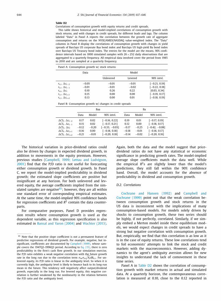
644 Z. Shi / Journal of Financial Economics 134 (2019) 617–646

Table D2

Correlations of consumption growth with equity returns and credit spreads.

This table shows historical and model-implied correlations of consumption growth with

stock returns, and with changes in credit spreads, for different leads and lags. The column

labeled “Data” in Panel A reports the correlation between the growth rate of aggregate

consumption and returns on the NYSE/AMEX/NASDAQ value-weighted index. The “Data”

columns in Panel B display the correlations of consumption growth with changes in yield

spreads of Barclays US corporate Baa bond index and Barclays US high-yield Ba bond index

over Barclays US Treasury bond index. The entries for the model are the means, 90% confi-

dence intervals based on 10 0 0 simulated samples with 26 × 252 daily observations that are

aggregated to a quarterly frequency. All empirical data involved cover the period from 1985

to 2010 and are sampled at a quarterly frequency.

Panel A: Consumption growth w/ stock returns

Data Model

Unlevered Levered 90% intvl.

r e,t , �c t−2 −0 .05 −0.01 −0.01 [ −0.21, 0.19]

r e,t , �c t−1 −0 .01 −0.01 −0.02 [ −0.22, 0.18]

r e,t , �c t 0 .10 0.26 0.22 [0.03, 0.34]

r e,t , �c t+1 0 .15 0.00 0.00 [ −0.19, 0.17]

r e,t , �c t+2 0 .13 0.00 0.01 [ −0.18, 0.19]

Panel B: Consumption growth w/ changes in credit spreads

Baa Ba

Data Model 90% intvl. Data Model 90% intvl.

�CS t , �c t−2 0 .17 0.02 [ −0.16, 0.22] 0.19 0.01 [ −0.17, 0.19]

�CS t , �c t−1 0 .15 0.02 [ −0.17, 0.21] 0.12 0.00 [ −0.18, 0.17]

�CS t , �c t −0 .12 −0.20 [ −0.33, −0.03] −0.17 −0.25 [ −0.42, −0.08]

�CS t , �c t+1 −0 .16 0.00 [ −0.18, 0.18] −0.18 −0.01 [ −0.18, 0.17]

�CS t , �c t+2 −0 .21 −0.01 [ −0.20, 0.18] −0.14 −0.02 [ −0.20, 0.16]

The historical variation in price-dividend ratios could

also be driven by changes in expected dividend growth, in

addition to movements in the equity premium. However,

previous studies ( Campbell, 1999; Lettau and Ludvigson,

2001 ) find that the P/D ratio is not useful for forecasting

either consumption growth or dividend growth. In Panel

C, we report the model-implied predictability in dividend

growth; the estimated slope coefficients are positive but

insignificant at any horizon. For both unlevered and lev-

ered equity, the average coefficients implied from the sim-

ulated samples are negative 65 ; however, they are all within

one standard error of corresponding empirical estimates.

At the same time, the model-implied 90% confidence bands

for regression coefficients and R 2 contain the data counter-

parts.

For comparative purposes, Panel D provides regres-

sion results where consumption growth is used as the

dependent variable, as this regression specification is also

estimated in Bansal and Yaron (2004) and Wachter (2013) .

65 Note that the positive slope coefficient is not a permanent feature of

predictive regressions of dividend growth. For example, negative, but in-

significant, coefficients are documented by Campbell (1999) , whose sam-

ple covers the 1947Q2-1996Q3 period. According to Eq. (15) , there is zero

predictability in the firm’s cash flow growth. In our simulation exercise,

the P/D ratio exhibits a weak negative correlation with the future growth

rate in the long run due to the correlation term σoa σa

√

A t dB A,t . For un-

levered equity, its P/D ratio is linear in the ambiguity level. So when it is

currently high, the ambiguity level is likely to bounce back to its long-run

mean in the future. This tendency will negatively affect output/dividend

growth, especially in the long run. For levered equity, this negative cor-

relation is further weakened by the nonlinearity in the relation between

the P/D ratio and the ambiguity level.

Again, both the data and the model suggest that price-

dividend ratios do not have any statistical or economic

significance in predicting growth rates. The model-implied

average slope coefficients match the data well. While

the empirical R 2 s are slightly lower than the model’s

predictions, they still fall within the 90% confidence

band. Overall, the model accounts for the absence of

predictability in dividend and consumption growth.

D.2. Correlations

Cochrane and Hansen (1992) and Campbell and

Cochrane (1999) point out that the weak correlation be-

tween consumption growth and stock returns in the

US data is inconsistent with the implications of many

consumption-based models. For models solely driven by

shocks to consumption growth, these two series should

be highly, if not perfectly, correlated. Similarly, if we sim-

ply embed a Merton model inside these equilibrium mod-

els, we would expect changes in credit spreads to have a

strong but negative correlation with consumption growth.

But, empirically, we find that this correlation is as low as it

is in the case of equity returns. These low correlations tend

to foil economists’ attempts to link the stock and credit

markets with the macroeconomics. However, adding dy-

namics to the agent’s ambiguity aversion allows for new

insights to understand the lack of comovement in these

time series.

Panel A in Table D2 shows the correlation of consump-

tion growth with market returns in actual and simulated

data. At a quarterly horizon, the contemporaneous corre-

lation is measured at 0.10, close to the 0.12 reported in

Z. Shi / Journal of Financial Economics 134 (2019) 617–646 645

Campbell and Cochrane (1999) . To account for this weak

correlation, exogenous shocks to the economy, besides con-

sumption shocks, are necessary. With innovations in the

ambiguity level, the model implies a mean correlation of

0.22 and a 90% confidence interval, which embrace the

empirical correlation coefficients.

When studying consumption’s correlation with credit

spreads, we examine the spreads for both investment-

grade and high-yield bonds. To disentangle variations in

the credit components of yield spreads, Panel B focuses on

the results of the lowest investment-grade rating, Baa, and

the highest speculative-grade rating, Ba. In the data, there

is a negative but weak correlation between spread changes

and economic fundamentals. In our model, changes in

credit spreads result only from uncertainty in ambiguity

innovations, and as such they should be orthogonal to con-

sumption growth without the correlation term. Incorporat-

ing the empirical comovement between the consumption

and ambiguity processes leads to correlation coefficients of

−0.20 and −0.25. The higher model-implied correlation for

high-yield bonds (compared to investment-grade ones) is

consistent with the data.

References

Aït-Sahalia, Y. , 1999. Transition densities for interest rate and other non-

linear diffusions. Journal of Finance 54 (4), 1361–1395 . Aït-Sahalia, Y. , 2002. Maximum likelihood estimation of discretely sam-

pled diffusions: A closed-form approximation approach. Econometrica70 (1), 223–262 .

Aït-Sahalia, Y. , 2008. Closed-form likelihood expansions for multivariatediffusions. Annals of Statistics 36, 906–937 .

Aït-Sahalia, Y. , 2012. User’s guide for the matlab library implementing

closed form mle for diffusions. Unpublished working paper, PrincetonUniversity .

Albagli, E. , Hellwig, C. , Tsyvinski, A. , 2013. Dynamic dispersed informationand the credit spread puzzle. Unpublished working paper, Yale Uni-

versity . Alili, L. , Kyprianou, A.E. , 2005. Some remarks on first passage of Lévy pro-

cesses, the American put and pasting principles. Annals of Applied

Probability 15 (3), 2062–2080 . Andersen, T.G. , Bollerslev, T. , Diebold, F.X. , Ebens, H. , 2001. The distribu-

tion of realized stock return volatility. Journal of Financial Economics61 (1), 43–76 .

Anderson, E.W. , Ghysels, E. , Juergens, J.L. , 2005. Do heterogeneous beliefsmatter for asset pricing? Review of Financial Studies 18 (3), 875–924 .

Anderson, E.W. , Ghysels, E. , Juergens, J.L. , 2009. The impact of risk and

uncertainty on expected returns. Journal of Financial Economics 94(2), 233–263 .

Anderson, E.W. , Hansen, L.P. , Sargent, T.J. , 2003. A quartet of semigroupsfor model specification, robustness, prices of risk, and model detec-

tion. Journal of the European Economic Association 1 (1), 68–123 . Ang, A. , Bekaert, G. , 2007. Stock return predictability: is it there? Review

of Financial Studies 20 (3), 651–707 .

Avramov, D. , Chordia, T. , Jostova, G. , Philipov, A. , 2007. Momentum andcredit rating. Journal of Finance 62 (5), 2503–2520 .

Avramov, D. , Jostova, G. , Philipov, A. , 2007. Understanding changes in cor-porate credit spreads. Financial Analysts Journal 63 (2), 90–105 .

Bakshi, G. , Panayotov, G. , Skoulakis, G. , 2012. The Baltic Dry Index asa predictor of global stock returns, commodity returns, and global

economic activity. In: Unpublished working paper, Temple Univer-sity, Hong Kong University of Science & Technology, and University

of British Columbia. .

Bansal, R. , Kiku, D. , Shaliastovich, I. , Yaron, A. , 2014. Volatility, the macroe-conomy, and asset prices. Journal of Finance 69 (6), 2471–2511 .

Bansal, R. , Shaliastovich, I. , 2013. A long-run risks explanation of pre-dictability puzzles in bond and currency markets. Review of Financial

Studies 26 (1), 1–33 . Bansal, R. , Yaron, A. , 2004. Risks for the long run: a potential resolution

of asset pricing puzzles. Journal of Finance 59 (4), 1481–1509 .

Benzoni, L. , Collin-Dufresne, P. , Goldstein, R.S. , 2005. Can standard prefer-ences explain the prices of out-of-the-money S&P 500 put options?

In: Unpublished working paper, NBER . Benzoni, L. , Collin-Dufresne, P. , Goldstein, R.S. , 2011. Explaining asset pric-

ing puzzles associated with the 1987 market crash. Journal of Finan-cial Economics 101 (3), 552–573 .

Bhamra, H.S. , Kuehn, L.-A. , Strebulaev, I.A. , 2010. The levered equity risk

premium and credit spreads: A unified framework. Review of Finan-cial Studies 23 (2), 645–703 .

Black, F. , 1976. Studies of stock price volatility changes. Proceedings of the1976 Meetings of the American Statistical Association, Business and

Economic Statistics 177–181 . Black, F. , Scholes, M. , 1973. The pricing of options and corporate liabilities.

Journal of Political Economy 81 (3), 637–654 . Boudoukh, J. , Michaely, R. , Richardson, M. , Roberts, M.R. , 2007. On the im-

portance of measuring payout yield: implications for empirical asset

pricing. Journal of Finance 62 (2), 877–915 . Boyarchenko, N. , 2012. Ambiguity shifts and the 20 07–20 08 financial cri-

sis. Journal of Monetary Economics 59 (5), 493–507 . Brekke, K.A. , Øksendal, B. , 1991. The high contact principle as a suffi-

ciency condition for optimal stopping. Stochastic Models and OptionValues: Applications to Resources, Environment, and Investment Prob-

lems. Emerald, Bingley, 187–208 .

Buraschi, A . , Jiltsov, A . , 2006. Model uncertainty and option markets withheterogeneous beliefs. Journal of Finance 61 (6), 2841–2897 .

Buraschi, A. , Piatti, I. , Whelan, P. , 2018. Rationality and subjective bondrisk premia. In: Unpublished working paper, Imperial College Business

School . Buraschi, A. , Trojani, F. , Vedolin, A. , 2014. Economic uncertainty, disagree-

ment, and credit markets. Management Science 60 (5), 1281–1296 .

Buraschi, A. , Whelan, P. , 2012. Term structure models with differencesin beliefs. In: Unpublished working paper, Imperial College Business

School . Campbell, J.Y. , 1999. Asset prices, consumption, and the business cycle.

Handbook of Macroeconomics. Elsevier, Amsterdam, 1231–1303 . Campbell, J.Y. , Cochrane, J.H. , 1999. By force of habit: A consump-

tion-based explanation of aggregate stock market behavior. Journal of

Political Economy 107 (2), 205–251 . Campbell, J.Y. , Shiller, R.J. , 1988. Stock prices, earnings, and expected div-

idends. Journal of Finance 43 (3), 661–676 . Campbell, J.Y. , Thompson, S.B. , 2008. Predicting excess stock returns out of

sample: can anything beat the historical average? Review of FinancialStudies 21 (4), 1509–1531 .

Campello, M. , Chen, L. , Zhang, L. , 2008. Expected returns, yield

spreads, and asset pricing tests. Review of Financial Studies 21 (3),1297–1338 .

Chen, H. , 2010. Macroeconomic conditions and the puzzles of creditspreads and capital structure. Journal of Finance 65 (6), 2171–2212 .

Chen, H. , Cui, R. , He, Z. , Milbradt, K. , 2018. Quantifying liquidity and de-fault risks of corporate bonds over the business cycle. Review of Fi-

nancial Studies 31 (3), 852–897 .

Chen, J. , Hong, H. , Stein, J.C. , 2002. Breadth of ownership and stock re-turns. Journal of Financial Economics 66 (2), 171–205 .

Chen, L. , Collin-Dufresne, P. , Goldstein, R. , 2009. On the relation betweenthe credit spread puzzle and the equity premium puzzle. Review of

Financial Studies 22 (9), 3367–3409 . Chen, Z. , Epstein, L. , 2002. Ambiguity, risk, and asset returns in continuous

time. Econometrica 70 (4), 1403–1443 . Christoffersen, P. , Du, D. , Elkamhi, R. , 2017. Rare disasters, credit, and op-

tion market puzzles. Management Science 63 (5), 1341–1364 .

Clark, T.E. , West, K.D. , 2007. Approximately normal tests for equal pre-dictive accuracy in nested models. Journal of Econometrics 138 (1),

291–311 . Cochrane, J.H. , Hansen, L.P. , 1992. Asset pricing explorations for macroe-

conomics. NBER Macroeconomics Annual 7, 115–165 . Collin-Dufresne, P. , Goldstein, R. , 2005. Improving on the Campbell-Shiller

Log-Linearization Approximation.. In: Unpublished working paper, UC

Berkeley and University of Minnesota . Cooper, I. , Priestley, R. , 2009. Time-varying risk premiums and the output

gap. Review of Financial Studies 22 (7), 2801–2833 . Dai, Q. , Singleton, K. , 20 0 0. Specification analysis of affine term structure

models. Journal of Finance 55 (5), 1943–1978 . David, A. , 2008. Inflation uncertainty, asset valuations, and the credit

spreads puzzle. Review of Financial Studies 21 (6), 2487–2534 .

Davydenko, S.A. , 2012. When do firms default? A study of the defaultboundary.. Unpublished working paper, University of Toronto .

Davydenko, S.A. , Strebulaev, I.A. , Zhao, X. , 2012. A market-based study ofthe cost of default. Review of Financial Studies 25 (10), 2959–2999 .

646 Z. Shi / Journal of Financial Economics 134 (2019) 617–646

Diether, K.B. , Malloy, C.J. , Scherbina, A. , 2002. Differences of opinion and the cross-section of stock returns. Journal of Finance 57 (5),

2113–2141 . Drechsler, I. , 2013. Uncertainty, time-varying fear, and asset prices. Journal

of Finance 68 (5), 1837–1883 . Du, D., Elkamhi, R., Ericsson, J., 2018. Time-varying asset volatility and the

credit spread puzzle. Journal of Finance doi: 10.1111/jofi.12765 .

Duffie, D. , 2001. Dynamic Asset Pricing Theory. Princeton University Press, Princeton .

Duffie, D. , Epstein, L. , 1992. Stochastic differential utility. Econometrica 60 (2), 353–394 .

Duffie, D. , Filipovi c, D. , Schachermayer, W. , 2003. Affine processes and ap- plications in finance. Annals of Applied Probability 13, 984–1053 .

Duffie, D. , Skiadas, C. , 1994. Continuous-time security pricing: a util- ity gradient approach. Journal of Mathematical Economics 23 (2),

107–132 .

Elkamhi, R. , Ericsson, J. , 2008. Time-varying risk premia in corporate bond markets. Unpublished working paper, University of Iowa .

Epstein, L.G. , Schneider, M. , 2003. Recursive multiple-priors. Journal of Economic Theory 113 (1), 1–31 .

Epstein, L.G. , Schneider, M. , 2007. Learning under ambiguity. Review of Economic Studies 74 (4), 1275–1303 .

Epstein, L.G. , Schneider, M. , 2008. Ambiguity, information quality, and as-

set pricing. Journal of Finance 63 (1), 197–228 . Epstein, L.G. , Schneider, M. , 2010. Ambiguity and asset markets. Annual

Review of Financial Economics 2 (1), 315–346 . Epstein, L.G. , Wang, T. , 1994. Intertemporal asset pricing under knightian

uncertainty. Econometrica 62 (2), 283–322 . Fama, E.F. , French, K.R. , 1988. Dividend yields and expected stock returns.

Journal of Financial Economics 22 (1), 3–25 .

Fama, E.F. , French, K.R. , 1989. Business conditions and expected returns on stocks and bonds. Journal of Financial Economics 25 (1), 23–49 .

Fama, E.F. , Schwert, G.W. , 1977. Asset returns and inflation. Journal of Fi- nancial Economics 5 (2), 115–146 .

Feldhütter, P. , Schaefer, S. , 2018. The myth of the credit spread puzzle. Review of Financial Studies 31, 2897–2942. .

Gagliardini, P. , Porchia, P. , Trojani, F. , 2009. Ambiguity aversion and the

term structure of interest rates. Review of Financial Studies 22 (10), 4157–4188 .

Gajdos, T. , Hayashi, T. , Tallon, J.-M. , Vergnaud, J.-C. , 2008. Attitude toward imprecise information. Journal of Economic Theory 140 (1), 27–65 .

Gilboa, I. , Schmeidler, D. , 1989. Maxmin expected utility with nonunique prior. Journal of Mathematical Economics 18 (2), 141–153 .

Goldstein, R. , Ju, N. , Leland, H. , 2001. An EBIT-Based Model of Dynamic

Capital Structure. Journal of Business 74 (4), 483–512 . Goyal, A. , Welch, I. , 2003. Predicting the equity premium with dividend

ratios. Management Science 49 (5), 639–654 . Hackbarth, D. , Miao, J. , Morellec, E. , 2006. Capital structure, credit risk,

and macroeconomic conditions. Journal of Financial Economics 82 (3), 519–550 .

Hansen, L.P. , Sargent, T.J. , 2001. Robust control and model uncertainty.

American Economic Review 91 (2), 60–66 . Hansen, L.P. , Sargent, T.J. , 2008. Robustness. Princeton university press,

Princeton. . He, Z. , Milbradt, K. , 2014. Endogenous liquidity and defaultable bonds.

Econometrica 82 (4), 1443–1508 . Heckman, J.J. , 1976. The common structure of statistical models of trunca-

tion, sample selection and limited dependent variables, and a simple estimator for such models. Annals of Economic and Social Measure-

ment 5 (4), 475–492 .

Heckman, J.J. , 1979. Sample selection bias as specification error. Econo- metrica 47 (1), 153–162 .

Hodrick, R.J. , 1992. Dividend yields and expected stock returns: alterna- tive procedures for inference and measurement. Review of Financial

Studies 5 (3), 357–386 . Huang, J.-Z. , Huang, M. , 2012. How much of the corporate-Treasury yield

spread is due to credit risk? Review of Asset Pricing Studies 2 (2),

153–202 . Illeditsch, P.K. , 2011. Ambiguous information, portfolio inertia, and excess

volatility. Journal of Finance 66 (6), 2213–2247 . Ilut, C. , 2012. Ambiguity aversion: Implications for the uncovered inter-

est rate parity puzzle. American Economic Journal: Macroeconomics 4 (3), 33–65 .

Ilut, C.L. , Schneider, M. , 2011. Ambiguous business cycles. Unpublished

working paper, Duke University . Ilut, C.L. , Schneider, M. , 2014. Ambiguous business cycles. American Eco-

nomic Review 104 (8), 2368–2399 . Jeong, D. , Kim, H. , Park, J.Y. , 2015. Does ambiguity matter? Estimating as-

set pricing models with a multiple-priors recursive utility. Journal of Financial Economics 115 (2), 361–382 .

Jones, C.S. , Tuzel, S. , 2013. New orders and asset prices. Review of Finan-cial Studies 26 (1), 115–157 .

Kim, D. , Kon, S.J. , 1994. Alternative models for the conditional het- eroscedasticity of stock returns. Journal of Business 67, 563–598 .

Klibanoff, P. , Marinacci, M. , Mukerji, S. , 2005. A smooth model of decisionmaking under ambiguity. Econometrica 73 (6), 1849–1892 .

Klibanoff, P. , Marinacci, M. , Mukerji, S. , 2009. Recursive smooth ambiguity

preferences. Journal of Economic Theory 144 (3), 930–976 . Le, A. , Singleton, K. , 2013. The structure of risks in equilibrium affine mod-

els of bond yields. Unpublished working paper, University of North Carolina at Chapel Hill. .

Le, A. , Singleton, K.J. , 2010. An equilibrium term structure model with re-cursive preferences. American Economic Review 100 (2), 557–561 .

Leland, H.E. , 1994. Bond prices, yield spreads, and optimal capital struc- ture with default risk. Unpublished working paper, University of Cali-

fornia at Berkeley .

Leland, H.E. , 1994. Corporate debt value, bond covenants, and optimal capital structure. Journal of Finance 49 (4), 1213–1252 .

Leland, H.E. , 1998. Agency costs, risk management, and capital structure. Journal of Finance 53 (4), 1213–1243 .

Lettau, M. , Ludvigson, S. , 2001. Consumption, aggregate wealth, and ex- pected stock returns. Journal of Finance 56 (3), 815–849 .

Liu, J. , Pan, J. , Wang, T. , 2005. An equilibrium model of rare-event premia

and its implication for option smirks. Review of Financial Studies 18 (1), 131–164 .

Longstaff, F.A. , Mithal, S. , Neis, E. , 2005. Corporate yield spreads: Defaultrisk or liquidity? New evidence from the credit default swap market.

Journal of Finance 60 (5), 2213–2253 . Maccheroni, F. , Marinacci, M. , Rustichini, A. , 2006. Dynamic variational

preferences. Journal of Economic Theory 128 (1), 4–44 .

Maenhout, P.J. , 2004. Robust portfolio rules and asset pricing. Review of Financial Studies 17 (4), 951–983 .

McQuade, T.J. , 2016. Stochastic Volatility and Asset Pricing Puzzles. Un- published working paper, Stanford University .

Merton, R.C. , 1969. Lifetime portfolio selection under uncertainty: the continuous-time case. Review of Economics and Statistics 51,

247–257 .

Merton, R.C. , 1971. Optimum consumption and portfolio rules in a contin- uous-time model. Journal of Economic Theory 3 (4), 373–413 .

Merton, R.C. , 1973. An intertemporal capital asset pricing model. Econo- metrica 41, 867–887 .

Merton, R.C. , 1974. On the pricing of corporate debt: the risk structure ofinterest rates. Journal of Finance 29 (2), 449–470 .

Miao, J. , 2009. Ambiguity, risk, and portfolio choice under incomplete in-

formation. Annals of Economics and Finance 10 (2), 257–279 . Miller, E.M. , 1977. Risk, uncertainty, and divergence of opinion. Journal of

Finance 32 (4), 1151–1168 . Mordecki, E. , 2002. Optimal stopping and perpetual options for Lévy pro-

cesses. Finance and Stochastics 6 (4), 473–493 . Newey, W.K. , West, K.D. , 1987. A simple, positive semi-definite, het-

eroskedasticity, and autocorrelation consistent covariance matrix.

Econometrica 55 (3), 703–708 . Øksendal, B. , 1990. The high contact principle in optimal stopping and

stochastic waves. Cinlar, E., Chung, K. L., Getoor, R. K., Fitzsimmons, P. J., Williams, R. J. (Eds.), Seminar on Stochastic Processes 1989.

Birkhäuser, Basel, 177–192 . Øksendal, B. , 2003. Stochastic differential equations: An introduction with

applications. Springer, Berlin . Reisz, A.S. , Perlich, C. , 2007. A market-based framework for bankruptcy

prediction. Journal of Financial Stability 3 (2), 85–131 .

Rossi, M. , 2014. Realized volatility, liquidity, and corporate yield spreads. Quarterly Journal of Finance 4 (01), 1–42 .

Shleifer, A. , Vishny, R.W. , 1992. Liquidation values and debt capacity: a market equilibrium approach. Journal of Finance 47 (4), 1343–1366 .

Strebulaev, I.A. , 2007. Do tests of capital structure theory mean what they say? Journal of Finance 62 (4), 1747–1787 .

Strzalecki, T. , 2013. Temporal resolution of uncertainty and recursive mod-

els of ambiguity aversion. Econometrica 81 (3), 1039–1074 . Tauchen, G. , Zhang, H. , Liu, M. , 1996. Volume, volatility, and leverage: a

dynamic analysis. Journal of Econometrics 74 (1), 177–208 . Wachter, J.A. , 2013. Can time-varying risk of rare disasters explain aggre-

gate stock market volatility? Journal of Finance 68 (3), 987–1035 . Yu, J. , 2011. Disagreement and return predictability of stock portfolios.

Journal of Financial Economics 99 (1), 162–183 .

van Zundert, J. , Driessen, J. , 2018. Are stock and corporate bond marketsintegrated? Evidence from expected returns. Unpublished working pa-

per, Tilburg University .