journal of la advanced supervised spectral classifiers for
TRANSCRIPT

JOURNAL OF LATEX CLASS FILES, VOL. 6, NO. 1, JANUARY 2007 1
Advanced Supervised Spectral Classifiers forHyperspectral Images: A Review
Pedram Ghamisi, Member, IEEE, Javier Plaza, Senior Member, IEEE, Yushi Chen, Member, IEEE, Jun Li, SeniorMember, IEEE, Antonio Plaza, Fellow, IEEE
Abstract—Hyperspectral image classification has been a vi-brant area of research in recent years. Given a set of observa-tions, i.e., pixel vectors in a hyperspectral image, classificationapproaches try to allocate a unique label to each pixel vector.However, the classification of hyperspectral images is a chal-lenging task due to a number of reasons such as the presence ofredundant features, or the imbalance between the limited numberof available training samples, as well as the high dimensionalityof the data. The aforementioned issues (among others) make thecommonly used classification methods designed for the analysisof gray scale, color, or multispectral images inappropriate forhyperspectral images. To this end, several spectral classifiers havebeen specifically developed for hyperspectral images or carriedout on such data. Among those approaches, support vectormachines, random forests, neural networks, deep approaches,and logistic regression-based techniques have gained a greatinterest in the hyperspectral community. This paper reviewsmost existing spectral classification approaches in the literature.Then, it critically compares the most powerful hyperspectralclassification approaches from different points of view, includingtheir classification accuracy, and computational complexity. Thepaper also provides several hints for readers about the logicalchoice of an appropriate classifier based on the application athand.
Index Terms—Hyperspectral Image Classification, SupportVector Machines, Random Forests, Neural Networks, ExtremeLearning Machine, Deep Learning, Multinomial Logistic Regres-sion.
I. INTRODUCTION
Imaging spectroscopy (also known as hyperspectral imag-ing) is an important technique in remote sensing. Hyper-spectral imaging sensors often capture data from the visiblethrough the near infrared wavelength ranges, thus providinghundreds of narrow spectral channels from the same area onthe surface of the Earth.
Pedram Ghamisi is with German Aerospace Center (DLR), Remote SensingTechnology Institute (IMF) and Technische Universitat Munchen (TUM),Signal Processing in Earth Observation, Munich, Germany (correspondingauthors e-mail: [email protected]).
Javier Plaza and Antonio Plaza are with the Department of Technology ofComputers and Communications, University of Extremadura, Spain
Yushi Chen is with the Department of Information Engineering, HarbinInstitute of Technology (e-mail: [email protected]).
Jun Li is with the Guangdong Provincial Key Laboratory of Urbanizationand Geo-simulation, Center of Integrated Geographic Information Analysis,School of Geography and Planning, Sun Yat-sen University, Guangzhou,510275, China. E-mail: [email protected].
This research has been supported by the Chinese 1000 people program Bunder project 41090427 and Guangdong Provincial Science Foundation underproject 42030397. This work is also partly supported by the Alexander vonHumboldt Fellowship for postdoctoral researchers.
These instruments collect data consisting of a set of pixelsrepresented as vectors, in which each element is a mea-surement corresponding to a specific wavelength. The sizeof each vector is equal to the number of spectral channelsor bands. Hyperspectral images usually consist of severalhundred spectral data channels for the same area on thesurface of the Earth, while in multispectral data the numberof spectral channels are usually up to tens of bands [1].The detailed spectral information collected by hyperspectralsensors increases the capability of discriminating betweendifferent land-cover classes with increased accuracy. A numberof operational hyperspectral imaging systems are currentlyavailable, providing a large volume of image data that canbe used for a wide variety of applications such as ecologicalscience, geological science, hydrological science, precisionagriculture and military applications.
Due to the detailed spectral information available from thehundreds of (narrow) bands collected by hyperspectral sensors,accurate discrimination of different materials is possible. Thisfact makes hyperspectral data a valuable source of informationto be fed to advanced classifiers. The output of the classifica-tion step is known as classification map.
Fig. 1 categorizes different groups of classifiers with respectto different criteria, followed by a brief description. Sinceclassification is a wide field of research and it is not feasibleto investigate all those approaches in a single paper, wetried to narrow down our description by excluding the greenparts in Fig. 1, which have been extensively covered in othercontributions. We reiterate that our main goal in this paperis to provide a comparative assessment and best practicerecommendations for the remaining contributions in Fig. 1.
With respect to the availability of training samples, classifi-cation approaches can be split into two categories, supervisedand unsupervised classifiers. Supervised approaches classifyinput data using a set of representative samples for eachclass, known as training samples. Training samples are usuallycollected either by manually labeling a small number of pixelsin an image or based on some field measurements [2]. Incontrast, unsupervised classification (also known as clustering)does not consider training samples. This type of approachesclassify the data only based on an arbitrary number of initial“cluster centers” that may be either user-specified or may bequite arbitrarily selected. During the processing, each pixel isassociated with one of the cluster centers based on a similaritycriterion [1, 3]. Therefore, pixels that belong to differentclusters are more dissimilar to each other compared to pixelswithin the same clusters [4, 5].

JOURNAL OF LATEX CLASS FILES, VOL. 6, NO. 1, JANUARY 2007 2
There is a vast amount of literature on unsupervised clas-sification approaches. Among those methods, Kmeans [6],ISODATA [7] and Fuzzy Cmeans [8] rank amongst the mostpopular unsupervised approaches. This set of approaches isknown for being very sensitive to its initial cluster config-uration and may be trapped into sub-optimal solutions [9].To address this issue, researchers have tried to improve theresilience of the Kmeans (and its family) by optimizing itwith bio-inspired optimization techniques [3]. Since super-vised approaches consider class specific information, whichis provided by training samples, they lead to more preciseclassification maps than unsupervised approaches. In additionto unsupervised and supervised approaches, semi-supervisedtechniques have been introduced [10, 11]. In this type ofmethods, the training is based on both labeled training samplesas well as unlabeled samples. In the literature, it has beenshown that the classification accuracy obtained with semi-supervised approaches can outperform that obtained by su-pervised classification.
In this paper, our focus is on supervised classificationapproaches. The remainder of this section is organized asfollows: First, we present the concept of supervised classifi-cation by setting some notations. Then, we discuss parametricversus nonparametric classification and address some specificchallenges for classification of hyperspectral data. Next, weprovide a detailed literature review followed by a brief com-ment on strategies for classification accuracy assessment. Thesection concludes with a summary of the main contributions ofthe paper as a prelude to the description of relevant techniquesin subsequent sections.
A. Supervised Classification of Hyperspectral Data
A hyperspectral data set can be seen as a stack of manypixel vectors, here denoted by x = (x1, ..., xd)
T , where drepresents the number of bands or the length of the pixelvector. A common task when interpreting remote sensingimages is to differentiate between several land cover classes. Aclassification algorithm is used to separate between differenttypes of patterns [5]. In remote sensing, classification isusually carried out in a feature space [12]. In general, theinitial set of features for classification contains the spectralinformation, i.e., the wavelength information for the pixels [1].In this space, each feature is presented as one dimension andpixel vectors can be represented as points in this d-dimensionalspace. A classification approach tries to assign unknown pixelsto one of y classes Ω = y1, y2, ..., yK, where K representsthe number of classes, based on a set of representative samplesfor each class referred to as training samples. The individualclasses are discriminated based either on the similarity to acertain class or by decision boundaries, which are constructedin the feature space [5].
B. Parametric versus Nonparametric Classification
From another perspective, classification approaches can besplit into parametric and non-parametric. For example, thewidely used supervised maximum likelihood classifier (MLC)is often applied in the parametric context. In that manner, the
MLC is based on the assumption that the probability densityfunction for each class is governed by the Gaussian distribution[13]. In contrast, nonparametric methods are not constrainedby any assumptions on the distribution of the input data. Hencetechniques such as SVMs, neural networks, decision trees,and ensemble approaches (including random forests) can beapplied even if the class conditional densities are not known orcannot be estimated reliably [1]. Therefore, for hyperspectraldata with a limited number of available training samples, suchtechniques may lead to more accurate classification results.
C. Challenges for the Classification of Hyperspectral Data
In this section, we discuss on some specific characteristicsof hyperspectral data, which make the classification stepchallenging.
1) Curse of Dimensionality: In [14–16], researchers havereported some distinguishing geometrical, statistical, andasymptotical properties of high-dimensional data throughsome experimental examples such as: (1) as dimensionalityincreases, the volume of a hypercube concentrates in corners,or (2) as dimensionality increases, the volume of a hyper-sphere concentrates in an outside shell. With respect to theseexamples, the following conclusions have been drawn:
• A high-dimensional space is almost empty, which impliesthat multivariate data in IR is usually in a lower dimen-sional structure. In other words, high-dimensional datacan be projected into a lower subspace without sacrificingconsiderable information in terms of class separability[1].
• Gaussian distributed data have a tendency to concentratein the tails while, uniformly distributed data have atendency to be concentrated in the corners, which makesthe density estimation of high-dimensional data for bothdistributions more difficult.
• Fukunaga [13] showed that there is a relation between therequired number of training samples and the number ofdimensions for different types of classifiers. The requirednumber of training samples is linearly related to thedimensionality for linear classifiers and to the square ofthe dimensionality for quadratic classifiers (e.g., GaussianMLC [13]).
• In [17], Landgrebe showed that too many spectral bandsmight be undesirable in terms of expected classificationaccuracy. When dimensionality (the number of bands)increases, with a constant number of training samples,a higher dimensional set of statistics must be estimated.In other words, although higher spectral dimensions in-crease the separability of the classes, the accuracy of thestatistical estimation decreases. This leads to a decrease inclassification accuracies beyond a number of bands. Forthe purpose of classification, these problems are relatedto the curse of dimensionality.
It is expected that, as dimensionality increases, more in-formation is demanded in order to detect more classes withhigher accuracy. At the same time, the aforementioned char-acteristics demonstrate that conventional techniques developed

JOURNAL OF LATEX CLASS FILES, VOL. 6, NO. 1, JANUARY 2007 3
Criteria Types Brief Description Whether training samples are used or not?
Supervised classifiers Supervised approaches classify input data using a set of representative samples for each class, known as training samples.
Unsupervised classifiers Unsupervised approaches, also known as clustering, do not consider the labels of training samples to classify the input data.
Semi-supervised classifiers
The training step in semi-supervised approaches is based on both labeled training samples and unlabeled samples.
Whether any assumption on the distribution of the input data is considered or not?
Parametric classifiers Parametric classifiers are based on the assumption that the probability density function for each class is known.
Non-parametric classifiers Non-parametric classifiers are not constrained by any assumptions on the distribution of input data.
Either a single classifier or an ensemble classifier is taken into account?
Single classifier classifiers In this type of approaches, a single classifier is taken into account to allocate a class label for a given pixel.
Ensemble (multi) classifier In this type of approaches, a set of classifiers (multiple classifiers) is taken into account to allocate a class label for a given pixel.
Whether the technique uses hard partitioning, in which each data point belongs to exactly one cluster or not?
Hard classifiers Hard classification techniques do not consider the continuous changes of different land cover classes from one to another.
Soft (fuzzy) classifiers Fuzzy classifiers model the gradual boundary changes by providing measurements of the degree of similarity of all classes.
If spatial information is taken into account?
Spectral classifiers This type of approaches consider the hyperspectral image as a list of spectral measurements with no spatial organization.
Spatial classifiers This type of approaches classify the input data using spatially adjacent pixels, based on either a crisp or adaptive neighborhood system.
Spectral-spatial classifiers Sequence of spectral and spatial information is taken into account for the classification of hyperspectral data.
Whether the classifier learns a model of the joint probability of the input and the labeled pixels?
Generative classifiers This type of approaches learns a model of the joint probability of the input and the labeled pixels, and makes the prediction using Bayes rules.
Discriminative classifiers This type of approaches learns conditional probability distribution, or learns a direct map from inputs to class labels.
Whether the classifier predicts a probability distribution over a set of classes, given a sample input?
Probabilistic classifiers This type of approaches is able to predict, given a sample input, a probability distribution over a set of classes.
Non- probabilistic classifiers
This type of approaches simply assign the sample to the most likely class that the sample should belong to.
Which type of pixel information is used?
Sub-pixel classifiers In this type of approaches, the spectral value of each pixel is assumed to be a linear or non-linear combination of endmembers (pure materials).
Per-pixel Input pixel vectors are fed to classifiers as inputs.
Object- based and Object-oriented classifiers
In this type of approaches, a segmentation technique allocates a label for each pixel in the image in such a way that pixels with the same label share certain visual characteristics. In this case, objects are known as underlying units after applying segmentation. Classification is conducted based on the objects instead of a single pixel.
Per-field classifiers This type of classifiers is obtained using a combination of RS and GIS techniques. In this context, raster and vector data are integrated in a classification. The vector data are often used to subdivide an image into parcels, and classification is based on the parcels.
Fig. 1. A terminology of classification approaches based on different criteria. In order to narrow down the research line of the paper, we intentionally avoidelaborate on the green parts.

JOURNAL OF LATEX CLASS FILES, VOL. 6, NO. 1, JANUARY 2007 4
for multispectral data may not be suitable for the classificationof hyperspectral data.
The aforementioned issues related to the high-dimensionalnature of the data have a dramatic influence on supervisedclassification techniques[18]. These techniques demand a largenumber of training samples (which is almost impossible toobtain in practice) in order to make a precise estimation. Thisproblem is even more severe when dimensionality increases.Therefore, classification approaches developed on hyperspec-tral data need to be capable of handling high dimensional datawhen only a limited number of training samples is available.
2) Uncertainties: Uncertainties generated at differentstages of data acquisition and classification procedure can dra-matically influence the classification accuaries and the qualityof the final classification map [19–22]. There are many reasonsfor such uncertainties, including atmospheric conditions at dataacquisition time, data limitation in terms of radiometric andspatial resolutions, mosaicing several images and many others.Image registration and geometric rectification cause positionuncertainty. Furthermore, algorithmic errors at the time ofcalibrating either atmospheric or topographic effects may leadto radiometric uncertainties [23].
3) Influence of Spatial Resolution: Classification accuraciescan be highly influenced by the spatial resolution of thehyperspectral data. A higher spatial resolution can significantlyreduce the mixed-pixel problem and detect more details of thescene. In [24], it was mentioned that classification accuraciesare the result of a tradeoff between two aspects. The first aspectrefers to the influence of boundary pixels on classificationresults. In this case, as spatial resolution becomes finer, thenumber of pixels falling on the boundary of different objectswill decrease. The second aspect refers to the increasedspectral variance of different land-covers associated with finerspatial resolution.
When we deal with low or medium spatial resolution opticaldata, the existence of many mixed pixels between differentland-cover classes is the main source of uncertainties, whichinfluence on classification results dramatically.
Fine spatial resolution can provide detailed informationabout shape and structure of different land-covers. Such infor-mation can also be fed to the classification system to furtherincrease classification accuracy values and improve the qualityof classification maps. The consideration of spatial informationinto the classification system is a vibrant research topic inthe hyperspectral community, and it has been investigated inmany works like [1, 25–29]. As mentioned, the considerationof spatial information in the classification system is out ofthe scope of this work, which focuses on supervised spectralclassifiers. However, the use of high resolution hyperspectralimages introduces some new problems, especially those causedby the presence of shadows, which leads to high spectralvariations within the same land-cover class. These disadvan-tages may decline classification accuracy if classifiers cannoteffectively handle such effects [30].
D. Literature ReviewIn this subsection, we briefly outline some of the most
popular supervised classification methods for hyperspectral
imagery. Some of these methods will be further detailed insubsequent sections of the paper.
1) Probabilistic approaches: A common subclass of clas-sifiers is based on probabilistic approaches. This group ofclassifiers use statistical terminologies to find the best class fora given pixel. In contrast with those algorithms, which simplyallocate a label with respect to a ”best” class, probabilisticalgorithms output a probability of the pixel being a memberof each of the possible classes [5, 13, 31]. The best class isnormally then selected as the one with the highest probability.
For instance, the multinomial logistic regression (MLR)classifier [32], which is able to model the posterior classdistributions in a Bayesian framework, supplies (in additionto the boundaries between the classes) a degree of plausibilityfor such classes [33]. Sparse MLR (SMLR), by adopting aLaplacian prior to enforce sparsity, leads to good machinegeneralization capabilities in hyperspectral classification [34,35], though with some computational limitations. The logisticregression via splitting and augmented Lagrangian (LORSAL)algorithm opened the door to processing of hyperspectralimages with median or big volume and a very large numberof classes, using a high number of training samples [36, 37].More recently, a subspace-based version of this classifier,called MLRsub [38], has also been proposed. The idea ofapplying subspace projection methods relies on the basicassumption that the samples within each class can approxi-mately lie in a lower dimensional subspace. The explorationof MLR, SMLR, LORSAL and MLRsub for hyperspectralmodel present two important advantages. On the one hand,with the advantages of good algorithm generalization and fastcomputation, MLR has beenh1 widely aq used to model thespectral information of hyperspectral data [39–48]. On theother hand, as the structure of MLR classifiers is very openand flexible, composite kernel learning [49, 50] and multiplefeature learning [51, 52] become active topics under the MLRmodel and lead to very competitive results for hyperspectralimage classification problems.
2) Neural networks: The use of neural networks in complexclassification scenarios is a consequence of their successfulapplication in the field of pattern recognition [53]. Particu-larly in the 1990s, neural network approaches attracted manyresearchers in the area of classification of hyperspectral images[54, 55]. The advantage of such approaches over probabilis-tic methods are mainly resulting from the fact that neuralnetworks do no need prior knowledge about the statisticaldistribution of the classes. The attractiveness of such increaseddue to the availability of feasible training techniques for non-linearly separable data [56], although their use has been tradi-tionally affected by their algorithmic and training complexity[57] as well as by the number of parameters that need to betuned.
Several neural network-based classification approaches havebeen proposed in the literature considering both supervisedand unsupervised, non-parametric approaches [58–62], be-ing feedforward neural network (FN)-based classifiers themost commonly adopted ones. FNs have been well studiedand widely used since the introduction of the well-knownbackpropagation algorithm (BP) [63], a first order gradient

JOURNAL OF LATEX CLASS FILES, VOL. 6, NO. 1, JANUARY 2007 5
method for parameter optimization, which presents two mainproblems: slow convergence and the possibility of falling inlocal minima, especially when the parameters of the networkare not properly fine-tuned. With the aim of alleviating thedisadvantages of the original BP algorithm, several secondorder optimization-based strategies, which are faster and needless input parameters, have been proposed in the literature[64, 65]. Recently, the extreme learning machine (ELM)learning algorithm has been proposed to train single hiddenlayer feedforward neural networks (SLFN) [66, 67]. Then,the concept has been extended to multi-hidden-layer networks[68], radial basis function networks (RBF) [69], and kernellearning [70]. The main characteristic of the ELM is that thehidden layer (feature mapping) is randomly fixed and need notto be iteratively tuned. ELM based networks are remarkablyefficient in terms of accuracy and computational complexityand has been successfully applied as nonlinear classifier forhyperspectral data providing comparable results with the state-of-the-art methodologies [71–74].
3) Kernel methods including support vector machines(SVMs): SVMs are another example of a supervised clas-sification approach, which has been widely used for theclassification of hyperspectral data due to their capability tohandle high dimensional data with a limited number of trainingsamples [1, 75, 76]. SVMs were originally introduced toclassify linear classification problems. In order to generalizethe SVM for non-linear classification problems, the so-calledkernel trick was introduced [77]. The sensitivity to the choiceof the kernel and regularization parameters are the mostimportant disadvantages of a kernel SVM. For the former,the Gaussian radial basis function (RBF) is widely used inremote sensing [77]. The latter is classically addressed usingcross-validation techniques using training data [78]. Gomezet. al proposed an approach by combining both labeled andunlabeled pixels using clustering and mean map kernel toincrease the classification accuracy and reliability of SVM[79]. In [80], a local k-nearest neighbor adaption was takeninto account to formulate localized variants of SVMs. Tuiaand Camps-Vallas proposed a regularization approach to tacklethe issue of kernel predetermination. The method was basedon the identification of kernel structures through analysis ofunlabeled pixels [81]. In [82], a so-called bootstrapped SVMwas proposed as a modification of the SVM. The trainingstrategy of the approach is as follows: an incorrectly classifiedtraining sample in a given learning step is removed from thetraining pool, re-assigned a correct label, and re-introducedinto the training set in the subsequent training cycles.
In addition to the SVM, a composite kernel framework forthe classification of hyperspectral images has been recentlyinvestigated. In [83], a linearly weighted composite kernelframework with SVMs has been used for the classificationof hyperspectral data. However, classification using compositekernels and SVMs demands convex combination of kernelsand a time-consuming optimization process. To overcomethese limitations, a generalized composite kernel frameworkfor spectral-spatial classification has been developed in [83].The MLR [84–86] has been also investigated as an alternativeto the SVM classifier for the construction of composite kernels,
and a set of generalized composite kernels, which can belinearly combined without any constraint of convexity, wereproposed.
4) Decision trees: Decision trees represent another subclassof nonparametric approaches, which can be used for bothclassification and regression. Safavian and Landgrebe [87]provided a good description of such classifiers. During theconstruction of a decision tree, the training set is progressivelysplit into an increasing number of smaller, more homogeneousgroups. This unique hierarchical concept is different fromother classification approaches, which generally use the entirefeature space at once and make a single membership decisionper class [88]. The relative structural simplicity of decisiontrees as well as the relatively short training time required (com-pared to methods that can be computationally demanding) arethe main advantages of such classifiers [1, 89, 90]. Moreover,decision tree classifiers make it possible to directly interpretclass membership decisions with respect to the impact ofindividual features [5]. Although a standard decision tree maybe deteriorated under some circumstances, its general conceptis of interest and the classifier performance can be furtherimproved in terms of classification accuracies by classifierensembles or multiple classifier systems [91, 92].
5) Ensemble methods (multiple classifiers): Traditionally,a single classifier was taken into account to allocate a classlabel for a given pixel. However, in most cases, the use of anensemble of classifiers (multiple classifiers) can be consideredin order to increase the classification accuracies [1]. In order todevelop an efficient multiple classifier, one needs to determinean effective combination of classifiers that is able to benefiteach other while avoiding the weaknesses of them [91]. Twohighly used multiple classifiers are boosting and bagging [91,93, 94], which were elaborated in detail in [1].
6) Random forests: Random forests (RFs) were first in-troduced in [95], and they represent a popular ensemblemethod for classification and regression. This classifier hasbeen widely used in conjunction with hyperspectral data sinceit does not assume any underlying probability distributionfor input data. Moreover, it can provide a good classificationresult in terms of accuracies in an ill-posed situation whenthere is no balance between dimensionality and number ofavailable training samples. In [96], Rotation Forest is proposedbased on the idea of RFs to encourage simultaneously bothmember diversities and individual accuracy within a classifierensemble. For a detailed description of this approach pleasesee [1, 92, 95, 97, 98].
7) Sparse representation classifiers (SRCs): Another im-portant development has been the use of SRCs with dictionary-based generative models [99, 100]. In this case, an inputsignal is represented by a sparse linear combination of samples(atoms) from a dictionary [99], where the training data isgenerally used as the dictionary. The main advantage of SRCsis that it avoids the heavy training procedure which a super-vised classifier generally conducts, and the classification isperformed directly on the dictionary. Given the availability ofsufficient training data some researchers have also developeddiscriminative as well as compact class dictionaries to improveclassification performance [101].
JOURNAL OF LATEX CLASS FILES, VOL. 6, NO. 1, JANUARY 2007 6
8) Deep learning: Deep learning is a kind of neural net-work with multi-layers, typically deeper than three layers,which tries to hierarchically learn the features of input data.Deep learning is a fast-growing topic, which has shownusefulness in many research areas, including computer visionand natural language processing [102]. In the context of remotesensing, some deep models have been proposed for hyperspec-tral data feature extraction and classification [103]. Stackedauto-encoder (SAE) and auto-encoder with sparse constrainwere proposed for hyperspectral data classification [104, 105].Later, another deep model, deep belief network (DBN), wasproposed for the classification of hyperspectral data [106].Very recently, an unsupervised convolutional neural network(CNN) was proposed for remote sensing image analysis, whichuses greedy layer-wise unsupervised learning to formulate adeep CNN model [107].
E. Classification Accuracy Assessment
Accuracy assessment is a crucial step to evaluate the effi-ciency and capability of different classifiers. There are manysources of errors such as: errors caused by the classificationalgorithm, position errors caused by the registration step,mixed pixels and unacceptable quality of training and testsamples. In general, it is assumed that the difference betweenthe classified image and reference data is because of theerrors caused by the classification algorithm itself [23]. Aconsiderable number of works and reviews on classificationaccuracy assessment have been conducted in the area of remotesensing [1, 108–113].
F. Contributions of the Paper
The main aim of this paper is to critically compare rep-resentative spectral-based classifiers (such as those outlinedin subsection I-D) from different perspectives. Without anydoubt, classification plays an important role for the analysisof hyperspectral data. There are many papers dealing withadvanced classifiers but, to the best of our knowledge, thereis no contribution in the literature that critically reviewsand compares advanced classifiers with each other, providingrecommendations on best practice when selecting a specificclassifier for a given application domain.
To make our research line more specific, in this paperwe only consider spectral and per-pixel based classifiers.In other words, spatial classifiers, fuzzy approaches, sub-pixel classifiers, object-based approaches, and per-field RS-GIS approaches are considered to be out of the scope of thepaper.
Compared to previous review papers such as [114] pub-lished in 2009, which provides a general review on theadvances in techniques for hyperspectral image processing tillthat date, this paper is specifically on spectral classifiers, whichincludes the most recent and advance spectral classificationapproaches in the hyperspectral community (with many newdevelopments since the previous publication of that paper).
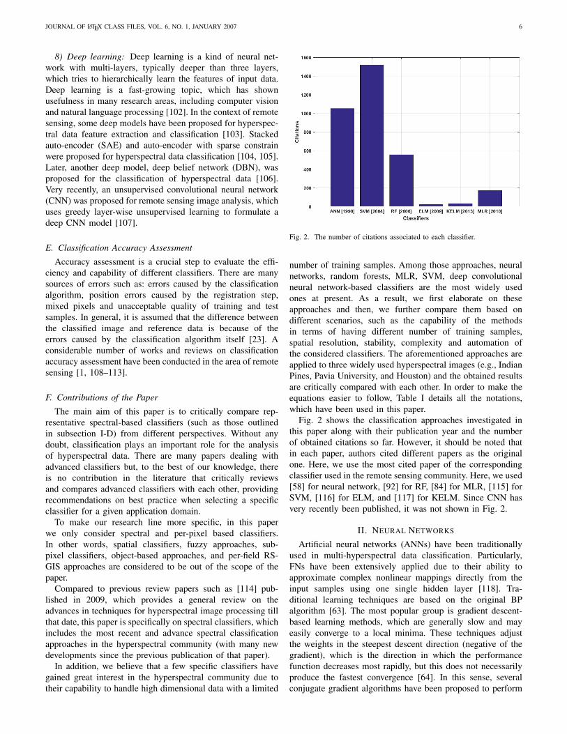
In addition, we believe that a few specific classifiers havegained great interest in the hyperspectral community due totheir capability to handle high dimensional data with a limited
Fig. 2. The number of citations associated to each classifier.
number of training samples. Among those approaches, neuralnetworks, random forests, MLR, SVM, deep convolutionalneural network-based classifiers are the most widely usedones at present. As a result, we first elaborate on theseapproaches and then, we further compare them based ondifferent scenarios, such as the capability of the methodsin terms of having different number of training samples,spatial resolution, stability, complexity and automation ofthe considered classifiers. The aforementioned approaches areapplied to three widely used hyperspectral images (e.g., IndianPines, Pavia University, and Houston) and the obtained resultsare critically compared with each other. In order to make theequations easier to follow, Table I details all the notations,which have been used in this paper.
Fig. 2 shows the classification approaches investigated inthis paper along with their publication year and the numberof obtained citations so far. However, it should be noted thatin each paper, authors cited different papers as the originalone. Here, we use the most cited paper of the correspondingclassifier used in the remote sensing community. Here, we used[58] for neural network, [92] for RF, [84] for MLR, [115] forSVM, [116] for ELM, and [117] for KELM. Since CNN hasvery recently been published, it was not shown in Fig. 2.
II. NEURAL NETWORKS
Artificial neural networks (ANNs) have been traditionallyused in multi-hyperspectral data classification. Particularly,FNs have been extensively applied due to their ability toapproximate complex nonlinear mappings directly from theinput samples using one single hidden layer [118]. Tra-ditional learning techniques are based on the original BPalgorithm [63]. The most popular group is gradient descent-based learning methods, which are generally slow and mayeasily converge to a local minima. These techniques adjustthe weights in the steepest descent direction (negative of thegradient), which is the direction in which the performancefunction decreases most rapidly, but this does not necessarilyproduce the fastest convergence [64]. In this sense, severalconjugate gradient algorithms have been proposed to perform
JOURNAL OF LATEX CLASS FILES, VOL. 6, NO. 1, JANUARY 2007 7
TABLE ITHE LIST OF NOTATIONS AND ACRONYMS.
Notations Definition Notations Definition Notations Definition Notations Definitionx Pixel vector d Number of bands b Bias λ Regularization parameterΦ Transformation C Regularization parameter υ Stack variable k Kernel||.|| Euclidean norm w Normal vector L Number of hidden nodes K Number of classesy Classification label w Input Weight n Number of training samples p(yi|xi) Probability of pixel iα Lagrange multiplier β Output weight v Visible units h Hidden units
a search along conjugate directions, which generally resultin faster convergence. These algorithms usually require highstorage capacity and are widely used in networks with largenumber of weights. Last, Newton’s based learning algorithmsgenerally provide better and fast optimization than conjugategradient methods. Based in the Hessian matrix (second deriva-tives) of the performance index at the current values of theweight and biases, their convergence is faster although theircomplexity usually introduce an extra computational burdenfor the calculation of the Hessian matrix.
Recently, the ELM algorithm has been proposed to trainsingle hidden layer feedforward neural networks [66, 67],which has emerged as an efficient algorithm that providesaccurate results in much less time. Traditional gradient-basedlearning algorithms assume that all the parameters (weightand bias) of the feedforward networks need to be tuned,establishing a dependency between different layers of param-eters and fostering very slow convergence. In [119, 120], itwas first shown that a SLFN (with N hidden nodes) withrandomly chosen input weights and hidden layer biases canexactly learn N distinct observations, which means that itmay not be necessary to adjust the input weights and firsthidden layer biases in applications. In [66], it was provedthat the input weights and hidden layer biases of a SLFN canbe randomly assigned if the activation function of the hiddenlayer is infinitely differentiable, which allow to determinate therest of parameters (weights between hidden and output layers)analytically, being the SLFN a linear system. This fact leadsto a significative decrease of the computational complexity ofthe algorithm, making it much faster than its predecessors, andturning ELM in the main alternative specially in the analysisof large amount of data.
Let (xiti) be n distinct samples where xi =[xi1, xi2, ..., xid]
T ∈ IRd and ti = [ti1, ti2, ..., tiK ]T ∈ IRK ,where d is the spectral dimensionality of the data and K thenumber of spectral classes. A SLFN with L hidden nodes andactivation function f(x) can be expressed as:
L∑i=1
βifi(xj) =
L∑i=1
βif(wi · xj + bi) = oj , j = 1, ..., n, (1)
where wi = [wi1, wi2, ..., wid]T is the weight vector con-
necting the ith hidden node and the input nodes, βi =[βi1, βi2, ..., βiK ]T is the weight vector connecting the ithhidden node and the output nodes, bi is the bias of the ithhidden node and f(wi ·xj +bi) is the output of the ith hiddennode regarding the input sample xi. The above equation canbe rewritten compactly as
H · β = Y, (2)
H =
f(w1 · x1 + b1) . . . f(wL · x1 + bL)
... . . ....
f(w1 · xn + b1) . . . f(wL · xn + bL)
L×L
, (3)
β =
βT1...βTL
L×K
,Y =
yT1
...yTL
n×K
(4)
where H is the output matrix of the hidden layer and β is theoutput weight matrix. The objective is to find specific wi, bi, β(i = 1, ..., L) so that:
||H(wi, bi)β −Y||2 =
minwi,bi,β ||H(w1, . . . ,wL, b1, . . . , bL)β −Y||2. (5)
As mentioned before, traditionally, the minimum of ||Hβ−Y||2 is calculated using gradient-based learning algorithms.The main issues related with these traditional methods are:
1) First and foremost, all gradient-based learning algo-rithms are very time-consuming in most applications.This became an important problem when classifyinghyperspectral data.
2) The size of the learning rate parameter strongly affectsthe performance of the network. Too small values gener-ate very slow convergence process while too large scoresin η make the learning algorithm became unstable andto diverge.
3) The error surface generally presents local minima.Gradient-based learning algorithms can get stuck at alocal minima. This can be an important issue if this localminima is far above a global minima.
4) FNs can be overtrained using BP-based algorithms, thusobtaining worse generalization performance. The effectsof overtraining can be alleviated using regularization orearly stopping criteria [121].
It has been proved in [66] that the input weights wi andthe hidden layer biases bi do not need to be tuned so that theoutput matrix of the hidden layer H can remain unchangedafter a random initialization. Fixing the input weights wi andthe hidden layer biases bi means that training an SLFN isequivalent to find a least-squares solution β of the linearsystem Hβ = Y. Different from the traditional gradient-based

JOURNAL OF LATEX CLASS FILES, VOL. 6, NO. 1, JANUARY 2007 8
learning algorithms, ELM aims to reach not only the smallesttraining error but also the smallest norm of output weights.
Minimize: ||Hβ −Y||2 and ||β||2. (6)
Let h(x) = [f(w1 ·x+b1), ..., f(wL ·x+bL)], if we expressequation (9) from the optimization theory point of view
minβ12 ||β||
22 + C 1
2
∑ni=1 ξ
2i , (7)
s.t. h(xi)β = yTi − ξ2i , i = 1, ..., n, (8)
where ξ2i is the training error of training sample xi and Cis a regularization parameter. The output of ELM can beanalytically expressed as
h(x)β = h(x)HT (I
C+ HHT )−1Y. (9)
This expression can be generalized to kernel version ofELM using the kernel trick [71]. The inner product operationconsidered in h(x)HT and HHT can be replaced by a kernelfunction: h(xi) · h(xj) = k(xi,xj). Both the regularized andkernel extensions of the traditional ELM algorithm require thesetting of the needed parameters (C and all kernel-dependentparameters). When compared with traditional learning algo-rithms, ELM has the following advantages:
1) There is no need to iteratively tuning the input weightswi and the hidden layer biases bi using slow gradient-based learning algorithms.
2) Derived from the fact that ELM tries to reach both thesmallest training error and the smallest norm of outputweights, this algorithm exhibits better generalization per-formance in most cases when compared with traditionalapproaches.
3) The learning speed of ELM is much faster than in thetraditional gradient-based learning algorithms. Depend-ing on the application, ELM can be tens to hundreds oftimes faster [66].
4) The use of ELM avoids inherent problems to gradient-descent methods such as getting stucked in a localminima or overfitting the model [66].
III. SUPPORT VECTOR MACHINES
Support vector machines (SVMs) [115] have been oftenused for the classification of hyperspectral data due to theircapability to handle high dimensional data with a limitednumber of training samples. The goal is to define an opti-mal linear separating hyperplane (the class boundary) withina multidimensional feature space that differentiates trainingsamples of two classes. The best hyperplane is the one thatleaves the maximum margin from both classes. The hyperplaneis obtained using an optimization problem that is solved viastructural risk minimization. In this way, in contrast withstatistical approaches, SVMs minimize classification error onunseen data without any prior assumptions made on theprobability distribution of the data [122].
The SVM tries to maximize the margins between the hy-perplane and the closest training samples [75]. In other words,in order to train the classifier only samples that are close to
the class boundary are needed to locate the hyperplane vector.This is why the closest training samples to the hyperplane arecalled support vector. More importantly, since only the closesttraining samples are influential on placing the hyperplane inthe feature space, SVM can classify the input data efficientlyeven if only a limited number of training samples is available[2, 115, 123, 124]. In addition, SVMs can efficiently handle theclassification of noisy patterns and multimodal feature spaces.
With regards to a binary classification problem in a d-dimensional feature space IRd, xi ∈ IRd, i =1, . . . , n is aset of n training samples with their corresponding class labelsyi ∈ 1,+1. The optimal separating hyperplane f(x) isdetermined by a normal vector w ∈ IRd and the bias b, where|b|/||w|| is the distance between the hyperplane and the origin,with ||w|| as the Euclidean norm from w:
f(x) = wx + b. (10)
The support vectors lie on two canonical hyperplanes wx +b = ±1 that are parallel to the optimal separating hyperplane.The margin maximization leads to the following optimizationproblem:
minw2
2+ C
n∑i
υi, (11)
where the slack variables υi and the regularization parameterC are considered to deal with misclassified samples in a nonseparable cases, i.e., cases that are not linearly separable. Theregularization parameter is a constant used as a penalty forsamples that lie on the wrong side of the hyperplane. It is ableto efficiently control the shape of the solution of the decisionboundary. Thus, it affects the generalization capability of theSVM (e.g., a large value of C may cause the approach tooverfit the training data) [97].
The SVM described above is a linear classifier, while deci-sion boundaries are often nonlinear for classification problems.To tackle this issue, kernel methods are required to extendthe linear SVM approach to nonlinear cases. In such cases,a nonlinear mapping is used to project the data into a high-dimensional feature space. After the transformation, the inputpattern x can be described by Φ(x).
(Φ(xi),Φ(xj)) = k(xi,xj). (12)
The transformation into the higher-dimensional space canbe computationally intensive. The computational cost can bedecreased using a positive definite kernel k, which fulfills theso-called Mercer’s conditions [77, 97]. When the Mercer’sconditions are met, the final hyperplane can be defined by
f(x) = (
n∑i=1
αiyik(xi,xj) + b), (13)
where αi denotes the Lagrange multipliers. For a detailedderivation of (13) we refer readers to [125]. In the new featurespace, an explicit knowledge of Φ is not needed. The onlyrequired knowledge lies on the kernel function k. Therefore,one needs to estimate the parameters of the kernel functionas well as the regularization parameter. To solve this issue, anautomatic model selection based on a cross-validation have

JOURNAL OF LATEX CLASS FILES, VOL. 6, NO. 1, JANUARY 2007 9
been introduced [126]. In [127], a genetic algorithm-basedapproach was used to regulate hyperplane parameters of anSVM while it finds efficient features to be fed to the classifier.
In terms of kernels, the Gaussian radial basis function (RBF)kernel may be the most widely used one in remote sensing[77, 97]. This kernel can handle more complex, nonlinear classdistributions in comparison with a simple linear kernel, whichis just a special case of the Gaussian RBF kernel [1, 128].
SVMs were originally developed for binary classificationproblems. In general, one needs to deal with multiple classesin remote sensing [1]. To address this, several multiclassstrategies have been introduced in the literature. Amongthose approaches, two main strategies are best-known, whichare based on the separation of the multiclass problem intoseveral binary classification problems [129]. These are theone-against-one strategy and the one-against-rest strategy [97].Some important points are listed bellow:
1) The capability of the SVM in handling a limited numberof training samples, self-adaptability, a swift trainingstage and easiness of the use are considered as themain advantages of this classifier. In addition, SVMsare resilient to getting trapped in local minima sincethe convexity of the cost function enables the classi-fier to consistently identify the optimal solution [122].More precisely, SVM deals with quadratic problemsand as a result, it guarantees to the global minimum.Furthermore, the result of the SVM is stable for thesame set of training samples and there is no need torepeat the classification step as this is a case for manyapproaches such as neural networks. Last but not least,SVMs are non-parametric, and do not assume a knownstatistical distribution of the data to be classified. This isconsidered as an important advantage due to the fact thatthe data acquired from remotely sensed imagery usuallyhave unknown distributions [122].
2) One drawback of the SVM lies on the setting of thekey parameters. For example, choosing a small valuefor the kernel width parameter may cause overfittingwhile a large value may cause oversmoothing, whichis a common drawback of all kernel-based approaches.Moreover, the choice of the regularization parameterC, which controls the trade-off between maximizingthe margin and minimizing the training error, is highlyimportant.
For further reading, a detailed introduction of SVM is givenby Burges [125], Cristianini and Shawe-Taylor [130], andScholkopf and Smola [77].
IV. MULTINOMIAL LOGISTIC REGRESSION (MLR)
The MLR models the posterior densities p(yi|xi,ω) asfollows [32]
p(yi = k|xi,ω) =exp(ω(k)T Φ(xi))∑Kk=1 exp(ω(k)T Φ(xi))
, (14)
where ω = [ω(1)T , ...,ω(K−1)T ]T are the logistic regressors.Again, yi is the class label of pixel xi ∈ Rd and d is thenumber of bands, K is the number of classes. Since the density
in (14) does not depend on translations of the regressors ω(k),we take ω(K) = 0. The term Φ(x) = [φ1(x), ..., φl(x)]T
is the fixed functions of the input, often termed features.The open structure of Φ(x) leads to the flexible selection ofthe input features, i.e, it can be linear, kernel and nonlinearfunctions. In order to control the algorithm complexity andits generalization capacity, the regressor ω is modeled as arandom vector with Laplacian density [131]:
p(ω) ∝ exp(−λ‖ω‖1), (15)
where λ is the regularization parameter controlling the degreeof sparsity of ω.
In the present problem, under a supervised scenario, learn-ing the class density amounts to estimating the logistic re-gressors ω, which can be done by computing the maximum aposterior (MAP) estimate of ω:
ω = arg maxω
`(ω) + log p(ω), (16)
where `(ω) is the log-likelihood function over the labeledtraining samples. For supervised learning, it is given by
`(ω) ≡n∑i=1
log p(yi = k|xi,ω), (17)
where n is the number of training samples. Problem (16),although convex, it is difficult to compute because the term of`(ω) is non-quadratic and the term log p(ω) is non-smooth.Following [32], `(ω) can be estimated by a quadratic function.However, the problem is still difficult as log p(ω) is non-smooth. This optimization problem (16) can be solved bythe SMLR in [131] and by the fast SMLR (FSMLR) in [35].However, most hyperspectral data sets are beyond the reachof these algorithms, as their processing becomes unbearablewhen the dimensionality of the input features increases. Thisis even more critical in the frameworks of composite kernellearning and multiple feature learning. In order to address thisissue, the LORSAL algorithm is proposed in [36, 37] to dealwith high-dimensional features and leads to good success inhyperspectral classification. For more information about theLORSAL algorithm, please see [33, 37].
The advantages of MLR are finally listed as follows:1) MLR classifiers are able to learn directly the posterior
class distributions and deal with the high dimensionalityof hyperspectral data in a very effective way. The classposterior probability plays a crucial role in the completeposterior probability under the Bayesian framework toinclude the spectral and spatial information.
2) The sparsity inducing prior on the regressors leads tosparse estimates, which allows us to control the algo-rithm complexity and their generalization capacity.
3) The open structure of the MLR results in a goodflexibility for the input functions, which can be linear,kernel-based and nonlinear.
V. RANDOM FORESTS (RFS)
RFs were proposed in [95] as an ensemble method forclassification and regression. Ensemble classifiers get theirname from the fact that several classifiers, i.e., an ensemble

JOURNAL OF LATEX CLASS FILES, VOL. 6, NO. 1, JANUARY 2007 10
of classifiers, are trained and their individual results are thencombined through a voting process [132, 133]. In other words,the classification label is allocated to the input vector (x)through yBrf = majority vote yb(x)B1 , where yb(x) is theclass prediction of the bth tree and B shows the total numberof trees. RFs can be considered as a particular case of decisiontrees. However, since RFs are composed of many classifiers, itinfers special characteristics that make it completely differentfrom a traditional classification trees and, therefore, it shouldbe understood as a new concept of classifiers [134].
The training algorithm for RFs applies the general techniqueof bootstrap aggregating, or bagging, to tree learners [94].Bootstrap aggregating is a technique used for training datacreation by resampling the original data set in a randomfashion with replacement (i.e., there is no deletion of the dataselected from the input sample for generating the next subset)[134]. The bootstrapping procedure leads to more efficientmodel performance since it decreases the variance of themodel without increasing the bias. In other words, while thepredictions of a single tree are highly sensitive to noise in itstraining set, the average of many trees is not that sensitive asfar as the trees are not correlated [135]. By training manytrees on a single training set, strongly correlated trees (oreven the same tree many times, if the training algorithm isdeterministic) are produced. Bootstrap sampling decorrelatesthe trees by showing them different training sets. RF usestrees as base classifiers, h(x, θk), k = 1, . . . , , where xand θk are the set of input vectors and the independent andidentically distributed random vectors [95, 136]. Since somedata may be used more than once for the training of theclassifier while some others may not be used, greater classifierstability is achieved. This makes the classifier more robustwhen a slight variations in input data occurs and consequently,higher classification accuracy can be obtained [134, 136].As mentioned in several studies such as [90, 91, 134, 137],methods based on bagging such as RFs, in contrast withother methods based on boosting, are not sensitive to noiseor overtraining.
In RFs, there are only two parameters in order to generatethe prediction model: the number of trees and the number ofprediction variable. The number of trees is a free parameter,which can be chosen with respect to the size and natureof the training set. One possible way to choose the optimalnumber of trees is based on cross-validation or by observingthe out-of-bag error [95, 133, 138]. For a detailed informationregarding RFs and their different implementations please see[1, 132, 133]. The number of prediction variable is referred tothe only adjustable parameter to which the forest is sensitive.As mentioned in [1], the “optimal” range of this parametercan be quite wide. However, the value is usually set approx-imately to the square root of the number of input features[132, 133, 139, 140].
Using RFs, the out-of-bag error, the variable importance,and proximity analysis, can be driven. In order to find detailedinformation about the RF and its derived parameters, pleasesee [1, 88, 95, 132, 133, 133, 138]. Below, some importantpoints of RFs are listed:
1) RFs are quite flexible and they can handle different
scenarios such as large number of attributes, very limitednumber of training samples, and small or large data sets.In addition, they are easy and quick to evaluate.
2) RFs do not assume any underlying probability distribu-tion for input data and can provide a good classificationresult in terms of accuracies, and can handle manyvariables and a lot of missing data. Another advantageof RF classifier is that it is insensitive to noise in thetraining labels. In addition, RF provides an unbiasedestimate of the test set error as trees are added to theensemble and finally it does not overfit.
3) The generated forest can be saved and used for otherdata sets.
4) In general, for sparse feature vectors, which is the casein most high dimensional data, a random selection offeatures may not be efficient all the time since uninfor-mative or correlated features might be selected whichdowngrades the performance of the classifier.
5) Although RFs have widely been used for classificationpurposes, a gap still remains between the theoreticalunderstanding of RFs and their corresponding practicaluse. A variety of RF algorithms have introduced showingpromising practical success. However, these algorithmsare difficult to analyze, and the basic mathematicalproperties of even the original variant are still not wellunderstood [141].
VI. DEEP LEARNING-BASED APPROACHES
There are some motivations to extract the invariant fea-tures from hyperspectral data. First, undesired scattering fromneighboring objects may deform the characteristics of the ob-ject of interest. Furthermore, different atmospheric scatteringconditions and intra-class variability make it extremely diffi-cult to extract the features effectively. Moreover, hyperspectraldata quickly increased in volume, velocity and variety, so it isdifficult to analyze in the complicated real situation. On theother hand, it is believed that deep models can progressivelylead to more invariant and abstract features at higher layers[102]. Therefore, deep models have the potential to be apromising tool. Deep learning involved a number of modelsincluding stacked auto-encoders (SAE) [142], deep beliefnetworks (DBN) [143], and deep convolutional neural network(CNN) [144].
A. Stacked Auto-Encoder (SAE)
Auto-encoder (AE) is the basic part of SAE [142]. As shownin Fig. 3, an AE contains one visible layer of d inputs, onehidden layer of L units, and one reconstruction layer of d units.During training procedure, x ∈ IRd is mapped to z ∈ IRL inthe hidden layer, and it is called “encoder”. Then, z is mappedto r ∈ IRd by a “decoder”, which is called “reconstruction”.These two steps can be formulated as:
z = f(wzx + bz),
r = f(wrx + br),
where wz and wr denote the input-to-hidden and the hidden-to-output weights, respectively. bz and br denote the bias

JOURNAL OF LATEX CLASS FILES, VOL. 6, NO. 1, JANUARY 2007 11
VII. DEEP LEARNING-BASED APPROACHES
A. Stacked Auto-encoder (SAE)
Auto-encoder (AE) is the basic part of SAE [7].As shown in Fig. 1, an AE contains one visible layer
of d inputs, one hidden layer of L units, and one reconstruction layer of d units.
During training procedure, 𝐱ϵℝ𝑑 is mapped to 𝐳ϵℝ𝐿 in the hidden layer, and it is called “encoder”.
Then, 𝐳 is mapped to 𝐫ϵℝ𝑑 by a “decoder”, which is called “reconstruction”. These two steps can be
formulated as:
𝐳 = 𝑓(𝐰z𝐱 + bz) (1)
𝐫 = 𝑓(𝐰r𝐱 + br) (2)
Where 𝐰z and 𝐰r denote the input-to-hidden and the hidden-to-output weights respectively, bz, br
denote the bias of hidden and output units, and 𝑓(∙) denotes the activation function.
Stacking the input and hidden layers of auto-encoders together layer by layer constructs a SAE. Fig.
2 shows a typical instance of a SAE connected with a subsequent logistic regression classifier. The
SAE can be used as a spectral classifier.
B. Deep Belief Networks (DBN)
Restricted Boltzmann machine (RBM) is a layer-wise training model in the construction of a DBN
wr, br
wz, bz
r
z
x
Reconstruction
Input
Fig. 1.Single hidden layer auto-encoder. The model learns a hidden feature “y” from input “x” by reconstructing it on “z”.
Pixel vectorHyperspectral data
AE AE
Logistic
regression
Stacked auto-encoers
Output:
Class labelsInput
Fig. 2.Spectral classifier based on SAE. The classification scheme shown here has 5 layers: one input layer, 2AEs and
alogistic regression layer.
Fig. 3. Single hidden layer auto-encoder. The model learns a hidden feature“z” from input “x” by reconstructing it on “r”.
Auto-encoder (AE) is the basic part of SAE [7].As shown in Fig. 1, an AE contains one visible layer
of d inputs, one hidden layer of L units, and one reconstruction layer of d units.
During training procedure, 𝐱ϵℝ𝑑 is mapped to 𝐳ϵℝ𝐿 in the hidden layer, and it is called “encoder”.
Then, 𝐳 is mapped to 𝐫ϵℝ𝑑 by a “decoder”, which is called “reconstruction”. These two steps can be
formulated as:
𝐳 = 𝑓(𝐰z𝐱 + 𝐛𝐳) (1)
𝐫 = 𝑓(𝐰r𝐱 + 𝐛𝐫) (2)
Where 𝐰z and 𝐰r denote the input-to-hidden and the hidden-to-output weights respectively, bz, br
denote the bias of hidden and output units, and 𝑓(∙) denotes the activation function.
Stacking the input and hidden layers of auto-encoders together layer by layer constructs a SAE. Fig.
2 shows a typical instance of a SAE connected with a subsequent logistic regression classifier. The
SAE can be used as a spectral classifier.
B. Deep Belief Networks (DBN)
Restricted Boltzmann machine (RBM) is a layer-wise training model in the construction of a DBN
[8]. As shown in Fig. 3, it is a two-layer network with“visible” units 𝒗 = 0,1𝑑 and “hidden”units
𝒉 = 0,1𝐿. A joint configuration of the units has an energy given by:
wr, br
wz, bz
r
z
x
Reconstruction
Input
Fig. 2. Single hidden layer auto-encoder. The model learns a hidden feature “z” from input “x” by reconstructing it on “r”.
Pixel vectorHyperspectral dataAE1 AE2
Logistic
regression
Stacked auto-encoder
Output:
Class labels
Input
Fig. 3. Spectral classifier based on SAE. The classification scheme shown here has 5 layers: one input layer, 2AEs and
alogistic regression layer.
Fig. 4. A typical instance of a SAE connected with a subsequent logisticregression classifier.
of hidden and output units, and f(.) denotes the activationfunction.
Stacking the input and hidden layers of auto-encoderstogether layer by layer constructs an SAE. Fig. 4 showsa typical instance of a SAE connected with a subsequentlogistic regression classifier. The SAE can be used as a spectralclassifier.
B. Deep Belief Networks (DBN)
Restricted Boltzmann machine (RBM) is a layer-wise train-ing model in the construction of a DBN [143]. As shownin Fig. 5, it is a two-layer network with “visible” unitsv = 0, 1d and “hidden” units h = 0, 1L. A jointconfiguration of the units has an energy given by:
E(v,h; θ) = −d∑i=1
bivi −L∑j=1
ajhj −d∑i=1
L∑j=1
wijvihj (18)
= −bTv− aTh− vTwh
where θ = bi, aj , wij, in which wij is the weight betweenvisible unit i and hidden unit j; bi and aj are bias terms ofvisible and hidden unit, respectively. The learning of wij isdone by a method called constructive divergence [143].
Due to the complexity of input hyperspectral data, RBM isnot the best way to capture the features. After the training ofRBM, the learnt features can be used as the input data for thefollowing RBM. This kind of layer-by-layer learning systemconstructs a DBN. As shown in Fig. 6, a DBN is employedfor feature learning and add a logistic regression layer abovethe DBN to constitute a DBN-logistic regression (DBN-LR)framework.
[8]. As shown in Fig. 3, it is a two-layer network with“visible” units 𝒗 = 0,1𝑑 and “hidden”units
𝒉 = 0,1𝐿. A joint configuration of the units has an energy given by:
𝐸(𝐯, 𝐡; θ) = − ∑ 𝑏𝑖𝑣𝑖 − ∑ 𝑎𝑗ℎ𝑗 − ∑ ∑ 𝑤𝑖𝑗𝑣𝑖ℎ𝑗
𝐹
𝑗=1
𝐷
𝑖=1
𝐿
𝑗=1
𝑑
𝑖=1
= −𝐛𝐓𝐯 − 𝐚𝐓𝐡 − 𝐯𝐓𝐰𝐡 (3)
where θ = 𝑏𝑖 , 𝑎𝑗 , 𝑤𝑖𝑗, 𝑤𝑖𝑗 is the weight between visible unit 𝑖 and hidden unit 𝑗; 𝑏𝑖 and 𝑎𝑗 are
bias terms of visible and hidden unit, respectively. The learning of 𝑤𝑖𝑗 is done by a method called
contrastive divergence [8].
h
v
w
Fig. 3.The illustration of restricted Boltzmann machine. The top layer represents the hidden units and the bottom layer represents
the visible units.
Due to the complexity of input hyperspectral data, RBM is not the best way to capture the features.
After the training of RBM, the learnt features can be used as the input data for the following RBM.
This kind of layer-by-layer learning system constructs a DBN. As shown in Fig.4, a DBN is employed
for feature learning and add a logistic regression layer above the DBN to constitute a DBN-logistic
regression (DBN-LR) framework.
C. Deep Convolutional Neural Network (CNN)
CNN is a special type of deep learning model which is inspired by neuroscience. A complete CNN
stage contains a convolution layer anda pooling layer. Deep CNN is constructed by stacking several
convolution layers and pooling layers to form adeep architecture. A convolutional layer is as follows:
𝐱𝑗𝑙 = 𝑓 (∑ 𝐱𝑖
𝑙−1 ∗
𝑀
𝑖=1
𝐤𝑖𝑗𝑙 + 𝑏𝑗
𝑙) (4)
where 𝐱𝑖𝑙−1 is the i-th feature map of (𝑙 − 1)-th layer, 𝐱𝑗
𝑙 is the 𝑗-th feature map of current (𝑖)-th
layer, and 𝑀 is the number of input feature maps. 𝐤𝑖𝑗𝑙 and 𝑏𝑗
𝑙 are the trainable parameters in the
Pixel vectorHyperspectral data
RBM RBM
Logistic
regression
DBN
Output:
Class labelsInput
Fig. 4.Spectral classifier based on DBN.
Fig. 5. Graphical illustration of a restricted Boltzmann machine. The toplayer represents the hidden units and the bottom layer represents the visibleunits
𝐸(𝐯, 𝐡; θ) = − ∑ 𝑏𝑖𝑣𝑖 − ∑ 𝑎𝑗ℎ𝑗 − ∑ ∑ 𝑤𝑖𝑗𝑣𝑖ℎ𝑗
𝐹
𝑗=1
𝐷
𝑖=1
𝐿
𝑗=1
𝑑
𝑖=1
= −𝐛𝐓𝐯 − 𝐚𝐓𝐡 − 𝐯𝐓𝐰𝐡 (3)
where θ = 𝑏𝑖 , 𝑎𝑗 , 𝑤𝑖𝑗, 𝑤𝑖𝑗 is the weight between visible unit 𝑖 and hidden unit 𝑗; 𝑏𝑖 and 𝑎𝑗 are
bias terms of visible and hidden unit, respectively. The learning of 𝑤𝑖𝑗 is done by a method called
contrastive divergence [8].
h
v
w
Fig. 4. The illustration of restricted Boltzmann machine. The top layer represents the hidden units and the bottom layer represents
the visible units.
Due to the complexity of input hyperspectral data, RBM is not the best way to capture the features.
After the training of RBM, the learnt features can be used as the input data for the following RBM.
This kind of layer-by-layer learning system constructs a DBN. As shown in Fig.5, a DBN is employed
for feature learning and add a logistic regression layer above the DBN to constitute a DBN-logistic
regression (DBN-LR) framework.
C. Deep Convolutional Neural Network (CNN)
CNN is a special type of deep learning model which is inspired by neuroscience. A complete CNN
stage contains a convolution layer with nonlinear operation and a pooling layer. Deep CNN is
constructed by stacking several convolution layers and pooling layers to form adeep architecture. A
convolutional layer is as follows:
𝐱𝑗𝑙 = 𝑓 (∑ 𝐱𝑖
𝑙−1 ∗
𝑀
𝑖=1
𝐤𝑖𝑗𝑙 + 𝐛𝑗
𝑙) (4)
where 𝐱𝑖𝑙−1 is the i-th feature map of (𝑙 − 1)-th layer, 𝐱𝑗
𝑙 is the 𝑗-th feature map of current (𝑖)-th
layer, and 𝑀 is the number of input feature maps. 𝐤𝑖𝑗𝑙 and 𝐛𝑗
𝑙 are the trainable parameters in the
convolutional layer. 𝑓(. ) is a nonlinear function and ∗ is the convolution operation.
Pooling operation offers invariance by reducing the resolution of the feature maps. The neuron in the
Pixel vectorHyperspectral data
RBM1 RBM2Logistic
regression
Output:
Class labels
Input
RBM3
Deep belief network
Fig. 5. Spectral classifier based on DBN. Fig. 6. A spectral classifier based on DBN. The classification scheme shownhere has four layers: one input layer, 2 RBMs, and a logistic regression layer.
C. Deep Convolutional Neural Network (CNN)
CNN is a special type of deep learning model which isinspired by neuroscience. A complete CNN stage contains aconvolution layer with nonlinear operation and a pooling layer.A convolutional layer is as follows 1:
xlj = f
(M∑i=1
xl−1i ∗ klij + blj
),
where xl−1i is the i-th feature map of (l-1)-th layer, xlj is the
j-th feature map of current (i)-th layer, and M is the numberof input feature maps. klij and blj are the trainable parametersin the convolutional layer. f(.) is a nonlinear function and ∗is the convolution operation.
Pooling operation offers invariance by reducing the reso-lution of the feature maps. The neuron in the pooling layercombines a small N × 1 patch of the convolution layer andthe most common pooling operation is max pooling.
A convolution layer, nonlinear function and pooling layerare three fundamental parts of CNNs [146]. By stackingseveral convolution layers with nonlinear operation and severalpooling layers, a deep CNN can be formulated. Deep CNN canhierarchically extract the features of inputs, which tend to beinvariant and robust [102].
The architecture of a deep CNN for spectral classificationis shown in Fig. 7. The input of the system is a pixel vectorof hyperspectral data and the output is the label of the pixel tobe classified. It consists of two convolutional and two poolinglayers as well as a logistic regression layer. After convolutionand pooling, the pixel vector can be converted into a featurevector, which captures the spectral information.
1It should be noted that we here explain 1D CNN as this paper deals withspectral classifiers. In order to find detailed information about 2D and 3DCNN for the classification of hyperspectral data, please see [145]

JOURNAL OF LATEX CLASS FILES, VOL. 6, NO. 1, JANUARY 2007 12
Conv.Pooling Logistic
regression
Feature map 1
Pixel vector Feature map 2
Feature map 3
Conv. Pooling StackOutput:
Class labels
Fig. 7. Spectral classifier based on deep CNN.
D. Discussion about deep learning approaches
The following aspects are worth being mentioned aboutdeep learning-based approaches:
1) Recently, some deep models have been employed intohyperspectral data feature extraction and classification.Deep learning opens a new window for future research,showcasing the deep learning-based methods’ huge po-tential [147].
2) The architecture design is the crucial part of a successfuldeep learning model. How to design a proper deep net isstill an open area in machine learning community, whilewe may use grid search to find a proper deep model.
3) Deep learning methods may lead to a serious problemcalled overfitting, which means that the results can bevery good on the training data but poor on the test data.To deal with the issue, it is necessary to use powerfulregularization methods.
4) Deep leaning methods can be combined with othermethods such as sparse coding and ensemble learning,which is another research area in hyperspectral dataclassification.
VII. EXPERIMENTAL RESULTS
This section describes our experimental results. First, we de-scribe the different hyperspectral data sets used in experiments.Then, we describe the setup for the different algorithms to becompared. We next present the obtained results and providea detailed discussion about the use of the different classifierstested in different applications.2
A. Data Description
1) Pavia University: This hyperspectral data set has beenrepeatedly used. This data set was captured on the city ofPavia, Italy by the ROSIS-03 (Reflective Optics Spectro-graphic Imaging System) airborne instrument. The flight overthe city of Pavia, Italy, was operated by the Deutschen Zen-trum fur Luft- und Raumfahrt (DLR, the German AerospaceAgency) within the context of the HySens project, managedand sponsored by the European Union. The ROSIS-03 sensorhas 115 data channels with a spectral coverage ranging from0.43 to 0.86 µm. Twelve channels have been removed dueto noise. The remaining 103 spectral channels are processed.
2The sets of training and test samples used in this paper are available onrequest by sending an email to the authors.
Asphalt
Meadows
Gravel
Trees
Metal sheets
Bare soil
Bitumen
Bricks
Shadows
(a) (b) (c)Fig. 8. ROSIS-03 Pavia University hyperspectral data. (a) Three band falsecolor composite, (b) Reference data and (c) Color code.
TABLE IIPAVIA UNIVERSITY: NUMBER OF TRAINING AND TEST SAMPLES.
Class Number of SamplesNo Name Total1 Asphalt 63042 Meadow 181463 Gravel 18154 Tree 29125 Metal Sheet 11136 Bare Soil 45727 Bitumen 9818 Brick 33649 Shadow 795
Total 40,002
The data have been corrected atmospherically, but not ge-ometrically. The spatial resolution is 1.3 m per pixel. Thedata set covers the Engineering School at the University ofPavia and consists of different classes including: trees, asphalt,bitumen, gravel, metal sheet, shadow, bricks, meadow and soil.This data set comprises 640 × 340 pixels. Fig. 8 presents afalse color image of ROSIS-03 Pavia University data and itscorresponding reference samples. These samples are usuallyobtained by manual labeling of a small number of pixels inan image or based on some field measurements. Thus, thecollection of these samples is expensive and time demanding[2]. As a result, the number of available training samples isusually limited, which is a challenging issue in supervisedclassification.

JOURNAL OF LATEX CLASS FILES, VOL. 6, NO. 1, JANUARY 2007 13
Grass/treesCorn-no till
Grass/pasture-mowed Corn-min till
Hay-windrowedCorn
OatsSoybeans-no till
WheatSoybeans-min till
WoodsSoybeans-clean till
Bldg-Grass-Tree-Drives Alfalfa
Stone-steel towers Grass/pasture
(a) (b) (c)Fig. 9. ROSIS-03 Pavia University hyperspectral data. (a) Three band falsecolor composite, (b) Reference data and (c) Color code.
TABLE IIIINDIAN PINES: NUMBER OF TRAINING AND TEST SAMPLES.
Class Number of SamplesNo Name Total1 Corn-notill 14342 Corn-mintill 8343 Corn 2384 Grass-pasture 4975 Grass-trees 7476 Hay-windrowed 4897 Soybean-notill 9688 Soybean-mintill 24689 Soybean-clean 61410 Wheat 21211 Woods 129412 Bldg-grass-tree-drives 38013 Stone-Steel-Towers 9514 Alfalfa 5415 Grass-pasture-mowed 2616 Oats 20
Total 10,366
2) Indian Pines: This data set was acquired by the AirborneVisible/Infrared Imaging Spectrometer (AVIRIS) sensor overthe agricultural Indian Pines test site in northwestern Indiana.The spatial dimensions of this data set are 145 × 145 pixels.The spatial resolution of this data set is 20m per pixel. Thisdata set originally includes 220 spectral channels but 20water absorption bands (104-108, 150-163, 220) have beenremoved, and the rest (200 bands) were taken into accountfor the experiments. The reference data contains 16 classes ofinterest, which represent mostly different types of crops andare detailed in Table III. Fig. 9 shows a three-band false colorimage and its corresponding reference samples.
3) Houston Data: This data set was captured by theCompact Airborne Spectrographic Imager (CASI) over theUniversity of Houston campus and the neighboring urban areain June, 2012. The size of the data is 349 × 1905 withthe spatial resolution of 2.5m. This data set is composed of144 spectral bands ranging 0.38-1.05m. This data consists of15 classes including: Grass Healthy, Grass Stressed, GrassSynthetic, Tree, Soil, Water, Residential, Commercial, Road,Highway, Railway, Parking Lot 1, Parking Lot 2, Tennis Courtand Running Track. The “Parking Lot 1” includes parkinggarages at the ground level and also in elevated areas, while“Parking Lot 2” corresponded to parked vehicles. Table IVdemonstrates different classes with the corresponding numberof training and test samples. Fig. 10 shows a three-band falsecolor image and its corresponding already-separated training
TABLE IVHOUSTON: NUMBER OF TRAINING AND TEST SAMPLES.
Class Number of SamplesNo Name Training Test1 Grass Healthy 198 10532 Grass Stressed 190 10643 Grass Synthetic 192 5054 Tree 188 10565 Soil 186 10566 Water 182 1437 Residential 196 10728 Commercial 191 10539 Road 193 105910 Highway 191 103611 Railway 181 105412 Parking Lot 1 192 104113 Parking Lot 2 184 28514 Tennis Court 181 24715 Running Track 187 473
Total 2,832 12,197
9
SVM RF RBFNN
(a) (b) (c)
(d) (e) (f)
Thematic classes:Healty grass Stressed grass Synthetic grass Tree SoilWater Residential Commercial Road HighwayRailway Parking lot 1 Parking lot 2 Tennis court Running track
Fig. 4: Classification maps corresponding to the worst (first row) and best (second row) classification overall accuracyachieved by the different classifiers for a single training and test set: (a) SVM with KPCA (OA=94.75%), (b) RF with Hyper(OA=94.57%), (c) RBFNN with KPCA (OA=90.08%), (d) SVM with SDAP(KPCA) (OA=98.39%), (e) RF with SDAP(kpca90+ I) + Ndsm (OA=97.51%), (f) RBFNN with SDAP(kpca90 + I) (OA=94.95% ).
Fig. 10. Houston - From top to bottom: A color composite representation ofthe hyperspectral data using bands 70, 50, and 20, as R, G, and B, respectively;Training samples; Test samples; and legend of different classes.
and test samples.
B. Algorithm Setup
In this paper two different scenarios are defined in order toevaluate different approaches. For the first scenario, trainingsamples have been chosen with different percentages from theavailable reference data. For this scenario, only Indian Pinesand Pavia University are taken into consideration. In this paper,1, 5, 10, 15, 20, and 25 percents of the whole samples havebeen randomly selected as training, except for classes alfalfa,grass-pasture-mowed and oats. These classes contain only asmall number of samples in the reference data. Therefore, only15 samples for each of these classes were chosen at randomas training samples and the rest as the test samples. For PaviaUniversity, 1, 5, 10, 15, and 20 percents of the whole sampleshave been randomly selected as training and the rest as testsamples. The experiments have been repeated 10 times, andthe mean and the standard deviation of the obtained overallaccuracy (OA) have been reported in the paper.

JOURNAL OF LATEX CLASS FILES, VOL. 6, NO. 1, JANUARY 2007 14
For the second scenario, the Houston data is taken intoaccount. The training and test samples of this data have beenseparated (Table IV). Results have been evaluated using OA,AA, K, and class specific accuracies.
The following classifiers have been investigated and com-pared in two different scenarios, discussed above:
• SVM (Support Vector Machine),• RF (Random Forest),• BP (Back Propagation Neural Network, also known as
Multilayer Perceptron),• ELM (Extreme Learning Machine),• KELM (Kernel Extreme Learning Machine),• 1D CNN (1-dimensional Convolutional Neural Network),• MLR (Multinomial Logistic Regression).
For the MLR classifier, which is executed by LORSALalgorithm [36, 37], we use a Gaussian Radial Basis Function(RBF) kernel given by K(x, z) = exp(−‖x − z‖2/2σ2),which is widely used in hyperspectral image classificationproblems [148]. For the parameters involved in the algorithm,we use the default settings provided in the online demo3,where it illustrates that the MLR classifier is insensitive tothe parameter settings, which also can be observed in thefollowing experiments.
In terms of the SVM, the RBF kernel is taken into account.The optimal hyperplane parameters C (parameter that controlsthe amount of penalty during the SVM optimization) and γ(spread of the RBF kernel) have been traced in the range ofC = 10−2, 10−1, ..., 104 and γ = 10−3, 10−2, ..., 104 usingfive-fold cross validation.
In terms of the RF, the number of trees is set to 300.The number of the prediction variable is set approximatelyto the square root of the number of input bands. The sameparameters have been used for all experiments stating that theRF is insensitive to the parameter initialization.
Regarding the BP-based neural network classifier (alsoknown as Multilayer Perceptron, MLP), the network has onlyone hidden layer and the number of hidden nodes has beenempirically set within the range (n+K)×2
3 ±10. The number ofinput nodes equals the number of spectral bands of the imagewhile the number of output nodes equals the number of spec-tral clasess. Hidden nodes have sigmoid activation functionswhile output nodes implement softmax activation function. Theimplemented learning algorithm is scaled conjugate gradientbackpropagation [64]. During the experiments, we empiricallyadjust the early stopping parameters to achieve reasonableperformance goals.
In the case of ELM, the network has also one singlehidden layer. The number of nodes L and the regulariza-tion parameter C [149] have been traced in the ranges ofL = 400, 600, 800, ..., 2000 and C = 10−3, 10−2, ..., 104
using five-fold cross validation.For the KELM, the RBF kernel is considered. Again, the
regularization parameter C and the kernel parameter γ havebeen searched in the ranges C = 10−3, 10−1, ..., 104 and γ =2−3, 2−2, ..., 24 also using five-cross validation.
3http://www.lx.it.pt/∼jun/demo LORSAL AL.rar.
1D CNN algorithm setup
For 1D CNN, the parameters including the kernel size, number of layers, number of feature maps,
number of neurons in hidden layer, learning rate are important to the final classification accuracy. Table
XX shows the architectures of deep 1D CNNs. As an example, for the Indian Pines data set there are 13
layers, denoted as I1, C2, S3, C4, S5, C6, S7, C8, S9, C10, S11, F12, and O13 in sequence. I1 is the
input layer. C refers to the convolution layers and S refers to pooling layers. F12 a fully-connected
layer, and O13 is the output layer of the whole neural network.
The input data are normalized into [-1 1]. The learning rate is set to 0.005, and the training epoch is 700
for Indian Pines data set. For Pavia University data set, we set the learning to 0.01, and the number of
epochs to 300. For CASI data set, the learning is 0.01 with 500 epochs.
Computational complexity
Generally speaking, deep learning methods are time-consuming in the procedure of training. Compare
to SVM, the training time of 1D deep CNN is about 2~3 times longer than RBF-SVM. On the other
hand, the advantage of deep CNN is that it is super-fast on testing.
Caption of Fig. 5 is wrong. The caption of Fig. 5 should be:
Fig. 5. Spectral classifier based on DBN. The classification scheme shown here has 4 layers: one input layer, 2 RBMs and a logistic regression
layer.
The line style of Fig. 10
TABLE XX THE ARCHITECTURES OF 1D CNN ON THREE DATA SETS
Layer Name I1 C2
S3
C4
S5
C6
S7
C8
S9
C10
S11 F12 O13
Kernel
Size
Indian
Pines 1×200
1×5
1×2
1×5
1×2
1×4
1×2
1×5
1×2
1×4
1×1
Fully
connected 1×16
Pavia
University 1×10³
1×8
1×2
1×7
1×2
1×8
1×2 - -
Fully
connected 1×9
Houston 1×144 1× 5
1×2
1×5
1×2
1×6
1×2
1×5
1×2 -
Fully
connected 1×15
Number of feature map/
number of neurons 6 12 24 48 96 256
Fig. 11. The Architectures of 1D CNN on Three Data Sets.
For 1D CNN, the important parameters are the kernelsize, number of layers, number of feature maps, number ofneurons in hidden layer, and learning rate. Figure 11 shows thearchitectures of the deep 1D CNN used for the experimentalpart. As an example, for the Indian Pines data set there are 13layers, denoted as I1, C2, S3, C4, S5, C6, S7, C8, S9, C10,S11, F12, and O13 in sequence. I1 is the input layer. C refersto the convolution layers and S refers to pooling layers. F12 afully-connected layer, and O13 is the output layer of the wholeneural network. The input data are normalized into [-1 1]. Thelearning rate is set to 0.005, and the training epoch is 700 forIndian Pines data set. For Pavia University data set, we setthe learning to 0.01, and the number of epochs to 300. Forthe Houston data set, the learning is 0.01 with 500 epochs.
Fig. 12 shows the overall accuracy of different approaches(i.e., the average value over 10 runs) on different percentagesof training samples on Indian Pines and Pavia University. Inorder to evaluate the stability of different classifiers on thechange of training samples, the standard deviation value over10 runs for each percentage is estimated and shown in Fig. 13.
For the Houston hyperspectral data, since the training andtest sets have been already separated, we performed theclassifiers on the standard set of training/test samples. Theclassification accuracies (i.e., overall accuracy (OA), averageaccuracy (AA), kappa coefficient (Kappa), and class specificaccuracies) are reported in Table V. The classification mapsof this data set are shown in Fig. 14.
C. Results and Discussion
The main observations obtained from our experimentalresults are listed systematically as follows:
• SVM vs. RF: Although both classifiers have the samenumber of hyperparameters to tune (i.e., RBF SVM hasγ and C, and RFs have the number of trees and the depthof the tree), RFs’ parameters are easier to set. In practice,the more trees we have the higher classification accuracyof RFs can be obtained. RFs are trained faster thankernel SVM. A suggested number of trees can be variedfrom 100 to 500 for the classification of hyperspectraldata. However, with respect to our experiments, the SVMestablished higher classification accuracies than RFs.
• SVM vs. BP: the SVM classifier presents the series ofadvantages over the BP classifier. The SVM exhibits less

JOURNAL OF LATEX CLASS FILES, VOL. 6, NO. 1, JANUARY 2007 15
computational complexity even when the kernel trick isused and, usually, provides better results when a smallnumber of training is available. However, if BP config-uration is properly tuned, both classifiers can providecomparable classification accuracies. Last but not least,the BP is much more complex from a computational pointof view. Actually, in this work we use the scaled conju-gate gradient backpropagation algorithm which presentsa practical complexity of O((n((dLK) +L+K))2) (thesquare of the number of weights of the network), where nthe number of training patterns, d the number of spectralbands, L the number of hidden nodes and K the numberof classes) [64].
• SVM vs. ELM: From an optimization point of view,ELM presents the same optimization cost function asleast square SVM (LS-SVM) [150] but much less com-putational complexity. In general terms, ELM training istens or hundreds of times faster than traditional SVM.Regarding the classification accuracy, it can be seen thatELM achieves comparable results.
• SVM vs. KELM: still in the case of kernel version ofELM, the computational complexity of SVM is muchbigger than KELM. It can be seen that KELM slightlyoutperforms SVM in terms of classification accuracy.Experimental validation shows that the kernel used inKELM and SVM is more efficient than the activationfunction used in ELM.
• BP vs. ELM vs. KELM: at the light of the results, itcan be seen how the three versions of the single layerfeedforward neural network provides competitive resultsin terms of accuracy. However, it should be noticed thatboth ELM and KELM are in the order of hundreds oreven thousands of times faster than BP. Actually, ELMand KELM have a practical complexity of O(L3+L2n+(K+d)Ln) and O(2n3 +(K+d)n2) respectively [151].
• SVM vs. 1D CNN: The main advantage of 2D and3D CNNs is that they use local connections to handlespatial dependencies. In this work, however, 1D CNN istaken into account to have a fair comparison with otherspectral approaches. In general, SVM can obtain higherclassification accuracies in a faster way than 1D CNN,so the use of SVMs over 1D CNN is recommended. Interms of CPU processing time, deep learning methods aretime-consuming in the training step. Compared to SVM,the training time of 1D deep CNN is about 2 or 3 timeslonger than RBF-SVM. On the other hand, the advantageof deep CNN is that it is extremely fast on the testingstage.
• Last but not least, some advantages of MLR (executed viaLORSAL) in comparison with other methods are listedas follows.
– It converges very fast and is relatively insensitiveto parameter settings. In our experiments, we usethe same settings for all data sets and receivedvery competitive results in comparison with thoseobtained from other methods.
– It has very low computational cost, with a practical
Fig. 12. Scenario 1 - Overall Accuracy: The overall accuracy of differentapproaches (i.e., the average value over 10 runs) on different percentages oftraining samples on Indian Pines and Pavia University obtained by differentclassification approaches.
complexity of O(d2(K − 1)).
For illustrative purposes, Fig. 12 provides a comparison ofthe different classifiers tested in this work with the IndianPines and Pavia University scenes (in terms of overall ac-curacy). As shown by Fig. 12, different classifiers providedifferent performances for the two considered images, indi-cating that there is no classifier consistently providing thebest classification results for different scenes. The stabilityof the different classifiers with the two considered scenes isillustrated in Fig. 13, which demonstrate how much a classifieris stable with respect to some changes on the available trainingsets. Furthermore, Table V gives detailed information aboutclassification accuracies obtained by different approaches ina different application domain, represented by the Houstondata set. In this case, the optimized classifiers also performsimilarly in terms of classification accuracy, so ultimately thechoice of a given classifier is more driven by the simplicity oftuning the parameters and configurations rather than the ob-tained classification results. This is an important observation,as it is felt that the hyperspectral community has reached apoint in which many classifiers are able to provide very highclassification accuracies. However, the competitive differencesbetween existing classifiers is more related to their simplicityand tuning configurations. In this regard, our assessment ofthe characteristics of different algorithms and their tuning isbelieved to provide helpful insights regarding the choice of agiven classifier in a certain application domain

JOURNAL OF LATEX CLASS FILES, VOL. 6, NO. 1, JANUARY 2007 16
1% 5% 10% 15% 20% 25%0
0.5
1
1.5
2
2.5
3
3.5
4
4.5
5
Training Samples (%)
Sta
ndar
d D
evia
tion
Indian Pines - Stability
RF
SVM
BP
ELM
KELM
1D CNN
MLR
1% 5% 10% 15% 20%0
0.2
0.4
0.6
0.8
1
1.2
1.4
Training Samples (%)
Sta
ndar
d D
evia
tion
Pavia University - Stability
RF
SVM
BP
ELM
KELM
1D CNN
MLR
Fig. 13. Scenario 1 - Stability: The standard deviation value over 10 runs ondifferent percentages of training samples on Indian Pines and Pavia Universityobtained by different classification approaches.
With the aforementioned observations in mind, we caninterpret the results provided in Table VI in more details. Inthis table, One bullet refers to the worst performance whilefour bullets refer to the best performance. It can be observedthat the KELM can provide high classification accuracies ina short period of time, while the obtained results are alsostable with respect to some changes of the input trainingsamples. SVM and MLR also show a fair balance betweenthe accuracy, automation (i.e., can be obtained with respect tothe number of parameters needs to be adjusted), speed (i.e., itwas evaluated based on the demanded CPU processing time ofdifferent classifiers), and stability, which can be advantageousfor applications where a trade-off between these elementsare needed. In contrast, 1D CNN does not show enoughadvantages neither in terms of classification accuracy andstability nor speed and automation.
VIII. CONCLUSIONS
In this paper, we have provided a review and criticalcomparison of different supervised hyperspectral classificationapproaches from different points of view, with particularemphasis on the configuration, speed and automation capac-ity of algorithms. The compared techniques include popularapproaches such as support vector machines, random forests,
TABLE VSCENARIO2: CLASSIFICATION ACCURACIES OBTAINED BY DIFFERENT
CLASSIFICATION APPROACHES ON THE HOUSTON HYPERSPECTRAL DATA.
Class SVM RF BP ELM KELM 1D CNN MLR
1 82.24 82.62 81.86 97.25 95.37 82.91 82.622 82.99 83.46 85.63 98.39 98.75 83.65 83.553 99.80 97.62 99.90 100.00 100.00 99.8 99.804 92.33 92.14 90.11 96.09 99.49 90.06 92.235 98.30 96.78 98.08 96.80 97.84 97.82 98.396 99.30 99.30 86.43 99.03 100.00 99.3 95.107 79.10 74.72 79.64 53.26 73.63 85.63 78.738 50.62 32.95 51.80 66.04 76.18 41.41 53.469 79.13 68.65 77.26 76.81 73.88 79.41 79.7910 57.92 43.15 57.46 71.39 76.08 53.38 58.1011 81.31 70.49 85.76 82.25 67.28 70.49 82.4412 76.08 55.04 81.76 72.21 59.74 72.72 76.3613 69.82 60.00 74.42 42.65 41.74 63.86 68.4214 100.00 99.19 99.31 89.81 90.41 99.6 98.7815 96.83 97.46 98.08 94.15 94.34 98.52 97.88OA 80.18 72.99 80.98 79.55 80.64 78.21 80.60AA 83.05 76.9 83.17 82.4 82.98 81.23 83.04
Kappa 0.7866 0.7097 0.7934 0.7783 0.7901 0.7846 0.7908
TABLE VIPERFORMANCE EVALUATION OF DIFFERENT SPECTRAL CLASSIFIERS IN
TERMS OF CLASSIFICATION ACCURACIES, SIMPLICITY AND SPEED,BEING CLOSER TO AUTOMATIC, AND STABILITY. ONE BULLET INFERS
THE WORST PERFORMANCE WHILE FOUR BULLETS INFER THE BESTPERFORMANCE.
Techniques Accuracy Automation Simplicity and Speed StabilityRF • • • •• • • •• ••
SVM • • •• • • • • • • • • •BP • • •• •• •• ••
ELM •• •• • • • • • •KELM • • •• •• • • • • • •
1D CNN •• • • ••MLR • • •• • • •• • • •• ••
neural networks, deep approaches, logistic regression-basedtechniques and sparse representation-based classifiers, whichhave been widely used in the hyperspectral analysis commu-nity but never investigated systematically using a quantitativeand comparative approach. The critical comparison conductedin this work leads to interesting hints about the logical choiceof an appropriate classifier based on the application at hand.The main conclusion that can be obtained from the presentstudy is that there is no classifier that consistently provides thebest performance among the considered metrics (particularly,from the viewpoint of classification accuracy), but ratherdifferent solutions that depend on the complexity of the anal-ysis scenario (i.e., availability of training samples, processingrequirements, tuning parameters, speed of the algorithm, etc.)and on the considered application domain. Combined, theinsights provided in this paper may facilitate the selectionof a specific classifier by an end-user depending on his/herexpentations and/or exploitation goals.
IX. ACKNOWLEDGMENT
The authors would like to thank the National Center forAirborne Laser Mapping (NCALM) for providing the Hous-ton data set. The ROSIS Pavia University and Indian Pinesdata and the corresponding reference information were kindly
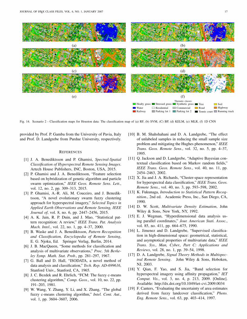
JOURNAL OF LATEX CLASS FILES, VOL. 6, NO. 1, JANUARY 2007 17
(a) (b)
(c) (d)
(e) (f)
9
SVM RF RBFNN
(a) (b) (c)
(d) (e) (f)
Thematic classes:Healty grass Stressed grass Synthetic grass Tree SoilWater Residential Commercial Road HighwayRailway Parking lot 1 Parking lot 2 Tennis court Running track
Fig. 4: Classification maps corresponding to the worst (first row) and best (second row) classification overall accuracyachieved by the different classifiers for a single training and test set: (a) SVM with KPCA (OA=94.75%), (b) RF with Hyper(OA=94.57%), (c) RBFNN with KPCA (OA=90.08%), (d) SVM with SDAP(KPCA) (OA=98.39%), (e) RF with SDAP(kpca90+ I) + Ndsm (OA=97.51%), (f) RBFNN with SDAP(kpca90 + I) (OA=94.95% ).
Fig. 14. Scenario 2 - Classification maps for Houston data: The classification map of (a) RF, (b) SVM, (C) BP, (d) KELM, (e) MLR, (f) 1D CNN
provided by Prof. P. Gamba from the University of Pavia, Italyand Prof. D. Landgrebe from Purdue University, respectively.
REFERENCES
[1] J. A. Benediktsson and P. Ghamisi, Spectral-SpatialClassification of Hyperspectral Remote Sensing Images.Artech House Publishers, INC, Boston, USA, 2015.
[2] P. Ghamisi and J. A. Benediktsson, “Feature selectionbased on hybridization of genetic algorithm and particleswarm optimization,” IEEE Geos. Remote Sens. Lett.,vol. 12, no. 2, pp. 309–313, 2015.
[3] P. Ghamisi, A.-R. Ali, M. Couceiro, and J. Benedik-tsson, “A novel evolutionary swarm fuzzy clusteringapproach for hyperspectral imagery,” Selected Topics inApplied Earth Observations and Remote Sensing, IEEEJournal of, vol. 8, no. 6, pp. 2447–2456, 2015.
[4] A. K. Jain, R. P. Duin, and J. Mao, “Statistical pat-tern recognition: A review,” IEEE Trans. Pat. AnalysisMach. Intel., vol. 22, no. 1, pp. 4–37, 2000.
[5] B. Waske and J. A. Benediktsson, Pattern Recognitionand Classification, Encyclopedia of Remote Sensing,E. G. Njoku, Ed. Springer Verlag, Berlin, 2014.
[6] J. B. MacQueen, “Some methods for classification andanalysis of multivariate observations,” Proc. 5th Berke-ley Symp. Math. Stat. Prob., pp. 281–297, 1967.
[7] G. Ball and D. Hall, “ISODATA, a novel method ofdata analysis and classification,” Tech. Rep. AD-699616,Stanford Univ., Stanford, CA, 1965.
[8] J. C. Bezdek and R. Ehrlich, “FCM: The fuzzy c-meansclustering algorithm,” Comp. Geos., vol. 10, no. 22, pp.191–203, 1981.
[9] W. Wang, Y. Zhang, Y. Li, and X. Zhang, “The globalfuzzy c-means clustering algorithm,” Intel. Cont. Aut.,vol. 1, pp. 3604–3607, 2006.
[10] B. M. Shahshahani and D. A. Landgrebe, “The effectof unlabeled samples in reducing the small sample sizeproblem and mitigating the Hughes phenomenon,” IEEETrans. Geos. Remote Sens., vol. 32, no. 5, pp. 4–37,1995.
[11] Q. Jackson and D. Landgrebe, “Adaptive Bayesian con-textual classification based on Markov random fields,”IEEE Trans. Geos. Remote Sens., vol. 40, no. 11, pp.2454–2463, 2002.
[12] X. Jia and J. A. Richards, “Cluster-space representationfor hyperspectral data classification,” IEEE Trans. Geos.Remote Sens., vol. 40, no. 3, pp. 593–598, 2002.
[13] K. Fukunaga, Introduction to Statistical Pattern Recog-nition., 2nd ed. Academic Press, Inc., San Diego, CA,1990.
[14] D. W. Scott, Multivariate Density Estimation, JohnWiley & Sons, New York, NY, 1992.
[15] E. J. Wegman, “Hyperdimensional data analysis us-ing parallel coordinates,” Jour. American Stati. Assoc.,vol. 85, no. 411, pp. 664–675, 1990.
[16] L. Jimenez and D. Landgrebe, “Supervised classifica-tion in high-dimensional space: geometrical, statistical,and asymptotical properties of multivariate data,” IEEETrans. Sys., Man, Cyber., Part C: Applications andReviews, vol. 28, no. 1, pp. 39–54, 1998.
[17] D. A. Landgrebe, Signal Theory Methods in Multispec-tral Remote Sensing. John Wiley & Sons, Hoboken,NJ, 2003.
[18] Y. Qian, F. Yao, and S. Jia, “Band selection forhyperspectral imagery using affinity propagation,” IETComput. Vis., vol. 3, no. 4, p. 213, 2009. [Online].Available: http://dx.doi.org/10.1049/iet-cvi.2009.0034
[19] F. Canters, “Evaluating the uncertainty of area estimatesderived from fuzzy landcover classification,” Photo.Eng. Remote Sens., vol. 63, pp. 403–414, 1997.

JOURNAL OF LATEX CLASS FILES, VOL. 6, NO. 1, JANUARY 2007 18
[20] J. L. Dungan, Toward a comprehensive view of uncer-tainty in remote sensing analysis, in, Uncertainty inRemote Sensing and GIS, 2nd ed. G. M. Foody and P.M. Atkinson (Eds), Chichester: John Wiley Sons, 2002.
[21] M. A. Friedl, K. C. McGwire, and D. K. Mciver, Anoverview of uncertainty in optical remotely sensed datafor ecological applications. C. T. Hunsaker, M. F.Goodchild, M.A. Friedl and T.J. Case (Eds), New York:Springer-Verlag, 2001.
[22] X. Wang, “Learning from big data with uncertainty ed-itorial,” Journal of Intelligent & Fuzzy Systems, vol. 28,no. 5, pp. 2329–2330, 2015.
[23] D. Lu and Q. Weng, “A survey of image classificationmethods and techniques for improving classificationperformance,” Int. Jour. Remote Sens., vol. 28, no. 5,pp. 823–870, 2007.
[24] C. E. Woodcock and A. H. Strahler, “The factor of scalein remote sensing,” Remote Sens. Env., vol. 21, no. 3,pp. 311–332, 1987.
[25] P. Ghamisi, M. Dalla Mura, and J. A. Benediktsson,“A survey on spectral–spatial classification techniquesbased on attribute profiles,” IEEE Trans. Geos. RemoteSens., vol. 53, no. 5, pp. 2335–2353, 2015.
[26] M. Fauvel, Y. Tarabalka, J. A. Benediktsson, J. Chanus-sot, and J. C. Tilton, “Advances in spectral-spatialclassification of hyperspectral images,” Proceedings ofthe IEEE, vol. 101, no. 3, pp. 652–675, 2013.
[27] C. Xu, H. Liu, W. Cao, and J. Feng, “Multispectralimage edge detection via clifford gradient,” ScienceChina Information Sciences, vol. 55, no. 2, pp. 260–269, jan 2012. [Online]. Available: http://dx.doi.org/10.1007/s11432-011-4540-0
[28] Z. Su, X. Luo, Z. Deng, Y. Liang, and Z. Ji, “Edge-preserving texture suppression filter based on jointfiltering schemes,” IEEE Trans. Multimedia, vol. 15,no. 3, pp. 535–548, apr 2013. [Online]. Available:http://dx.doi.org/10.1109/TMM.2012.2237025
[29] Z. Zhu, S. Jia, S. He, Y. Sun, Z. Ji, and L. Shen, “Three-dimensional Gabor feature extraction for hyperspectralimagery classification using a memetic framework,”Information Sciences, vol. 298, pp. 274–287, 2015.
[30] J. L. Cushnie, “The interactive effect of spatial resolu-tion and degree of internal variability within land-covertypes on classification accuracies,” Int. Jour. RemoteSens., vol. 8, pp. 15–29, 1987.
[31] Y. Zhong, Q. Zhu, and L. Zhang, “Scene classificationbased on the multifeature fusion probabilistic topicmodel for high spatial resolution remote sensingimagery,” IEEE Trans. Geosci. Remote Sensing, vol. 53,no. 11, pp. 6207–6222, nov 2015. [Online]. Available:http://dx.doi.org/10.1109/TGRS.2015.2435801
[32] D. Bohning, “Multinomial logistic regression algo-rithm,” Ann. Inst. Statist. Math., vol. 44, pp. 197–200,1992.
[33] J. Li, J. Bioucas-Dias, and A. Plaza, “Semi-supervisedhyperspectral image segmentation using multinomiallogistic regression with active learning,” IEEE Trans.Geosci. and Remote Sens., vol. 48, pp. 4085–4098,
2010.[34] P. Zhong, P. Zhang, and R. Wang, “Dynamic learning
of smlr for feature selection and classification of hyper-spectral data,” IEEE Geoscience and Remote SensingLetters, vol. 5, no. 2, pp. 280–284, April 2008.
[35] J. S. Borges, J. M. Bioucas-Dias, and A. R. S. Mar-cal, “Bayesian hyperspectral image segmentation withdiscriminative class learning,” IEEE Transactions onGeoscience and Remote Sensing, vol. 49, no. 6, pp.2151–2164, June 2011.
[36] J. Bioucas-Dias and M. Figueiredo, “Logistic regressionvia variable splitting and augmented Lagrangian tools,”Instituto Superior Tecnico, TULisbon, Tech. Rep., 2009.
[37] J. Li, J. Bioucas-Dias, and A. Plaza, “Hyperspectralimage segmentation using a new Bayesian approachwith active learning,” IEEE Trans. Geosci. and RemoteSens., vol. 49, no. 19, pp. 3947–3960, 2011.
[38] ——, “Spectral-spatial hyperspectral image segmen-tation using subspace multinomial logistic regressionand markov random fields,” IEEE Trans. Geosci. andRemote Sens., vol. 50, no. 3, pp. 809–823, 2012.
[39] P. Zhong and R. Wang, “Learning conditional randomfields for classification of hyperspectral images,” IEEETransactions on Image Processing, vol. 19, no. 7, pp.1890–1907, July 2010.
[40] Y. Qian, M. Ye, and J. Zhou, “Hyperspectral imageclassification based on structured sparse logistic regres-sion and three-dimensional wavelet texture features,”IEEE Transactions on Geoscience and Remote Sensing,vol. 51, no. 4, pp. 2276–2291, April 2013.
[41] P. Zhong and R. Wang, “Jointly learning the hybrid crfand mlr model for simultaneous denoising and classifi-cation of hyperspectral imagery,” IEEE Transactions onNeural Networks and Learning Systems, vol. 25, no. 7,pp. 1319–1334, July 2014.
[42] M. Khodadadzadeh, J. Li, A. Plaza, and J. M. Bioucas-Dias, “A subspace-based multinomial logistic regres-sion for hyperspectral image classification,” IEEE Geo-science and Remote Sensing Letters, vol. 11, no. 12, pp.2105–2109, Dec 2014.
[43] J. Li, J. M. Bioucas-Dias, and A. Plaza, “Spectral-spatialclassification of hyperspectral data using loopy beliefpropagation and active learning,” IEEE Transactions onGeoscience and Remote Sensing, vol. 51, no. 2, pp.844–856, Feb 2013.
[44] M. Khodadadzadeh, J. Li, A. Plaza, H. Ghassemian,J. M. Bioucas-Dias, and X. Li, “Spectral-spatial classifi-cation of hyperspectral data using local and global prob-abilities for mixed pixel characterization,” IEEE Trans-actions on Geoscience and Remote Sensing, vol. 52,no. 10, pp. 6298–6314, Oct 2014.
[45] L. Sun, Z. Wu, J. Liu, L. Xiao, and Z. Wei, “Supervisedspectral-spatial hyperspectral image classification withweighted markov random fields,” IEEE Transactions onGeoscience and Remote Sensing, vol. 53, no. 3, pp.1490–1503, March 2015.
[46] S. Sun, P. Zhong, H. Xiao, and R. Wang, “An mrfmodel-based active learning framework for the spectral-

JOURNAL OF LATEX CLASS FILES, VOL. 6, NO. 1, JANUARY 2007 19
spatial classification of hyperspectral imagery,” IEEEJournal of Selected Topics in Signal Processing, vol. 9,no. 6, pp. 1074–1088, Sept 2015.
[47] J. Li, M. Khodadadzadeh, A. Plaza, X. Jia, and J. M.Bioucas-Dias, “A discontinuity preserving relaxationscheme for spectral-spatial hyperspectral image classi-fication,” IEEE Journal of Selected Topics in AppliedEarth Observations and Remote Sensing, vol. 9, no. 2,pp. 625–639, Feb 2016.
[48] J. Zhao, Y. Zhong, H. Shu, and L. Zhang, “High-resolution image classification integrating spectral-spatial-location cues by conditional random fields,”IEEE Transactions on Image Processing, vol. 25,no. 9, pp. 4033–4045, sep 2016. [Online]. Available:http://dx.doi.org/10.1109/TIP.2016.2577886
[49] J. Li, P. Marpu, A. Plaza, J. Bioucas-Dias, and J. A.Benediktsson, “Generalized composite kernel frame-work for hyperspectral image classification,” IEEETrans. Geosci. and Remote Sens., 2013, in press.
[50] Y. Zhang and S. Prasad, “Locality preserving compositekernel feature extraction for multi-source geospatialimage analysis,” IEEE Journal of Selected Topics inApplied Earth Observations and Remote Sensing, vol. 8,no. 3, pp. 1385–1392, March 2015.
[51] J. Li, X. Huang, P. Gamba, J. M. Bioucas-Dias,L. Zhang, J. A. Benediktsson, and A. Plaza, “Multiplefeature learning for hyperspectral image classification,”IEEE Transactions on Geoscience and Remote Sensing,vol. 53, no. 3, pp. 1592–1606, March 2015.
[52] C. Zhao, X. Gao, Y. Wang, and J. Li, “Efficientmultiple-feature learning-based hyperspectral imageclassification with limited training samples,” IEEETransactions on Geoscience and Remote Sensing,vol. 54, no. 7, pp. 4052–4062, July 2016.
[53] C. Bishop, Pattern Recognition and Machine Learning.New York, NY, USA: Springer-Verlag, 2006.
[54] J. A. Benediktsson, P. H. Swain, and O. K. Ersoy,“Conjugate gradient neural networks in classification ofvery high dimensional remote sensing data,” Int. Jour.Remote Sens., vol. 14, no. 15, pp. 2883–2903, 1993.
[55] H. Yang, F. V. D. Meer, W. Bakker, and Z. J. Tan,“A back—propagation neural network for mineralogicalmapping from AVIRIS data,” Int. Jour. Remote Sens.,vol. 20, no. 1, pp. 97–110, 1999.
[56] J. A. Benediktsson, “Statistical methods and neural net-work approaches for classification of data from multiplesources,” Ph.D. dissertation, PhD thesis, Purdue Univ.,School of Elect. Eng. West Lafayette, IN, 1990.
[57] J. A. Richards, “Analysis of remotely sensed data: Theformative decades and the future,” IEEE Trans. Geos.Remote Sens., vol. 43, no. 3, pp. 422–432, 2005.
[58] J. A. Benediktsson, P. H. Swain, and O. K. Ersoy,“Neural network approaches versus statistical methodsin classification of multisource remote sensing data,”IEEE Transactions on Geoscience and Remote Sensing,vol. 28, no. 4, pp. 540–552, 1990.
[59] E. Merenyi, W. H. Farrand, J. V. Taranik, and T. B.Minor, “Classification of hyperspectral imagery with
neural networks: comparison to conventional tools,”Eurasip Journal on Advances in Signal Processing, vol.2014, no. 1, pp. 1–19, 2014.
[60] F. D. Frate, F. Pacifici, G. Schiavon, and C. Solimini,“Use of neural networks for automatic classificationfrom high-resolution images,” IEEE Transactions onGeoscience and Remote Sensing, vol. 45, no. 4, pp.800–809, 2007.
[61] F. Ratle, G. Camps-Valls, and J. Wetson, “Semisuper-vised neural networks for efficient hyperspectral imageclassification,” IEEE Transactions on Geosciences andRemote Sens., vol. 48, no. 5, pp. 2271–2282, 2010.
[62] Y. Zhong and L. Zhang, “An adaptive artificial im-mune network for supervised classification of multi-/hyperspectral remote sensing imagery,” IEEE Transac-tions on Geosciences and Remote Sens., vol. 50, no. 3,pp. 894–909, 2012.
[63] D. E. Rumelhart, G. E. Hinton, and R. J. Williams,“Learning representations by back-propagating errors,”Nature, vol. 323, no. 6088, pp. 533–536, 1986.
[64] M. Moller, “A scaled conjugate gradient algorithm forfast supervised learning,” Neural Networks, vol. 6, no. 4,pp. 525–533, 1993.
[65] M. T. Hagan and M. Menhaj, “Training feed-forwardnetworks with the marquardt algorithm,” IEEE Trans-actions on Neural Networks, vol. 5, no. 6, pp. 989–993,1994.
[66] G.-B. Huang, Q.-Y. Zhu, and C.-K. Siew, “Extremelearning machine: Theory and applications,” Neurocom-puting, vol. 70, pp. 489–501, 2006.
[67] G. Huang, G.-B. Huang, S. Song, and K. You, “Trendsin extreme learning machines: A review,” Neural Net-works, vol. 61, pp. 32–48, 2015.
[68] J. Tang, C. Deng, and G.-B. Huang, “Extreme learningmachine for multilayer perceptron,” IEEE Transactionson Neural Networks, 2015.
[69] G.-B. Huang and C.-K. Siew, “Extreme learning ma-chine: Rbf network case,” in Control, Automation,Robotics and Vision Conference, 2004. ICARCV 20048th, vol. 2, 2004, pp. 1029–1036.
[70] G.-B. Huang, “An insight into extreme learning ma-chines: Random neurons, random features and kernels,”Cognitive Computation, vol. 6, pp. 376–390, 2014.
[71] Y. Zhou, J. Peng, and C. L. P. Chen, “Extreme learningmachine with composite kernels for hyperspectral im-age classification,” IEEE Journal of Selected Topics inApplied Earth Observations and Remote Sens., vol. 8,no. 6, pp. 2351–2360, 2015.
[72] A. B. amd A. Araujo and D. Menotti, “Combiningmultiple classification methods for hyperspectral datainterpretation,” IEEE Journal of Selected Topics inApplied Earth Observations and Remote Sens., vol. 6,no. 3, pp. 1450–1459, 2013.
[73] J. Li, Q. Du, W. Li, and Y. Li, “Optimizing extremelearning machine for hyperspectral image classifica-tion,” Journal of Applied Remote Sensing, vol. 9, no. 1,p. 097296, 2015.
[74] A. Samat, P. Du, S. Liu, and L. Cheng, “E2lms:

JOURNAL OF LATEX CLASS FILES, VOL. 6, NO. 1, JANUARY 2007 20
Ensemble extreme learning machines for hyperspectralimage classfication,” IEEE Journal of Selected Topics inApplied Earth Observations and Remote Sens., vol. 7,no. 4, pp. 1060–1069, 2014.
[75] V. N. Vapnik, Statistical learning theory. John Wiley& Sons, New York, NY, 1998.
[76] B. Pan, J. Lai, and L. Shen, “Ideal regularizationfor learning kernels from labels,” Neural Networks,vol. 56, pp. 22–34, aug 2014. [Online]. Available:http://dx.doi.org/10.1016/j.neunet.2014.04.003
[77] B. Scholkopf and A. J. Smola, Learning with Kernels.MIT Press, Cambridge, MA, 2002.
[78] M. Fauvel, J. Chanussot, and J. A. Benediktsson, “Ker-nel principal component analysis for the classficationof hyperspectral remote-sensing data over urban areas,”EURASIP Jour. Adv. Signal Proc., pp. 1–14, 2009.
[79] L. Gmez-Chova, G. Camps-Valls, J. Muoz-Mar, andJ. Calpe, “Semisupervised image classification withlaplacian support vector machines,” IEEE Geos. RemoteSens. Let., vol. 5, no. 3, pp. 336–340, 2008.
[80] E. Blanzieri and F. Melgani, “Nearest neighbor classifi-cation of remote sensing images with the maximal mar-gin principle,” IEEE Geos. Remote Sens. Let., vol. 46,no. 6, pp. 1804–1811, 2008.
[81] D. Tuia and G. Camps-vallas, “Semisupervised remotesensing image classification with cluster kernels,” IEEEGeos. Remote Sens. Let., vol. 6, no. 2, pp. 224–228,2005.
[82] C. Castillo, I. Chollett, and E. klein, “Enhanced duck-weed detection using bootstrapped svm classificationon medium resolution rgb modis imagery,” Int. Jour.Remote Sens., vol. 29, no. 19, pp. 5595–5604, 2008.
[83] J. Li, P. Marpu, A. Plaza, J. Bioucas-Dias, and J. A.Benediktsson, “Generalized composite kernel frame-work for hyperspectral image classification,” IEEETrans. Geos. Remote Sens., vol. 51, no. 9, pp. 4816–4829, 2013.
[84] J. Li, J. Bioucas-Dias, and A. Plaza, “Semi-supervisedhyperspectral image segmentation using multinomiallogistic regression with active learning,” IEEE Trans.Geos. Remote Sens., vol. 48, no. 11, pp. 4085–4098,2010.
[85] ——, “Hyperspectral image segmentation using a newBayesian approach with active learning,” IEEE Trans.Geos. Remote Sens., vol. 49, no. 10, pp. 3947–3960,2011.
[86] B. Krishnapuram, L. Carin, M. Figueiredo, andA. Hartemink, “Sparse multinomial logistic regres-sion: Fast algorithms and generalization bounds,” IEEETrans. Pat. Analysis Mach. Intell., vol. 27, no. 6, pp.957–968, 2005.
[87] S. R. Safavian and D. Landgrebe, “A survey of decisiontree classifier methodology,” IEEE Trans. Syst, Man,Cyber., vol. 21, no. 3, pp. 294–300, 1991.
[88] L. Breiman, J. H. Friedman, R. Olshen, and C. J. Stone,Classification and Regression Tree. Chapman andHall/CRC, London, England, 1984.
[89] M. A. Friedl and C. E. Brodley, “Decision tree classifi-
cation of land cover from remotely sensed data,” RemoteSens. Env., vol. 61, no. 3, pp. 399–409, 1997.
[90] M. Pal and P. Mather, “An assessment of the effective-ness of decision tree methods for land cover classifica-tion,” Remote Sens. Env., vol. 86, no. 4, pp. 554–565,2003.
[91] G. J. Briem, J. A. Benediktsson, and J. R. Sveinsson,“Multiple classifiers applied to multisource remote sens-ing data,” IEEE Trans. Geos. Remote Sens., vol. 40,no. 10, pp. 2291–2299, 2003.
[92] P. O. Gislason, J. A. Benediktsson, and J. R. Sveinsson,“Random forests for land cover classification,” Pat.Recog. Lett., vol. 27, no. 4, pp. 294–300, 2006.
[93] L. Breiman, “Arcing classifier,” Ann. Statist., vol. 26,no. 3, pp. 801–849, 1998.
[94] ——, “Bagging predictors,” Mach. Learn., vol. 24,no. 1, pp. 123–140, 1994.
[95] ——, “Random forests,” Mach. Learn., vol. 45, no. 1,pp. 5–32, 2001.
[96] J. Xia, P. Du, X. He, and J. Chanussot, “Hyperspectralremote sensing image classification based on rotationforest,” IEEE Geos. Remote Sens. Let., vol. 11, no. 1,pp. 239–243, 2014.
[97] B. Waske, J. A. Benediktsson, K. Arnason, and J. R.Sveinsson, “Mapping of hyperspectral AVIRIS datausing machine-learning algorithms,” Canadian Jour.Remote Sens., vol. 35, pp. 106–116, 2009.
[98] Z. Zhi-Hua, Ensemble Methods: Foundations and Al-gorithms. Chapman and Hall/CRC, New York, NY,2012.
[99] Y. Chen, N. M. Nasrabadi, and T. D. Tran, “Hy-perspectral image classification using dictionary-basedsparse represenation,” IEEE Trans. Geosci. and RemoteSensing, vol. 49, no. 10, pp. 3973–3985, Oct. 2011.
[100] Z. Lai, W. K. Wong, Y. Xu, C. Zhao, andM. Sun, “Sparse alignment for robust tensor learning,”IEEE Trans. Neural Netw. Learning Syst., vol. 25,no. 10, pp. 1779–1792, oct 2014. [Online]. Available:http://dx.doi.org/10.1109/TNNLS.2013.2295717
[101] A. Castrodad, Z. Xing, J. Greer, E. Bosch, L. Carin,and G. Sapiro, “Learning discriminative sparse repre-sentations for modeling, source separation, and mappingof hyperspectral imagery,” IEEE Trans. Geosci. RemoteSensing, vol. 49, no. 11, pp. 4263–4281, Dec. 2011.
[102] Y. Bengio, A. Courville, and P. Vincent, “Representationlearning. a review and new perspectives,” IEEE Trans.Patt. Anal. Mach. Intell., vol. 35, no. 8, pp. 1798–1828,2013.
[103] L. G. Chova, D. Tuia, G. Moser, and G. C. Valls,“Multimodal classification of remote sensing images:A review and future directions,” Proc. IEEE, vol. 103,no. 9, pp. 1560–1584, 2015.
[104] Y. Chen, Z. Lin, X. Zhao, G. Wang, and Y. Gu,“Deep learning-based classification of hyperspectraldata,” IEEE Jour. Sel. Top. App. Earth Obs. RemoteSens., vol. 7, no. 6, pp. 2094 – 2107, 2014.
[105] C. Tao, H. Pan, Y. Li, and Z. Zou, “Unsupervised spec-tralspatial feature learning with stacked sparse autoen-

JOURNAL OF LATEX CLASS FILES, VOL. 6, NO. 1, JANUARY 2007 21
coder for hyperspectral imagery classification,” IEEEGeos. Remote Sens. Lett., vol. 12, no. 12, pp. 2438 –2442, 2015.
[106] Y. Chen, X. Zhao, and X. Jia, “Spectra-spatial clas-sification of hyperspectral data based on deep beliefnetwork,” IEEE Jour. Sel. Top. App. Earth Obs. RemoteSens., vol. 8, no. 6, pp. 2381–2292, 2015.
[107] A. Romero, C. Gatta, and G. C. Valls, “Unsuperviseddeep feature extraction for remote sensing image clas-sification,” IEEE Trans. Geos. Remote Sens., vol. 54,no. 3, pp. 1–14, 2016.
[108] J. A. Richards and X. Jia, Remote Sensing Digital ImageAnalysis, fourth, 2006 ed. Berlin: Springer-Verlag,1986.
[109] P. C. Smits, S. G. Dellepiane, and R. A. Schowengerdt,“Quality assessment of image classification algorithmsfor land-cover mapping: a review and a proposal for acostbased approach,” Int. Jour. Remote Sens., vol. 20,pp. 1461–1486, 1999.
[110] W. D. Hudson and C. W. RAMM, “Correct formulationof the kappa coefficient of agreement,” Photo. Eng.Remote Sens., vol. 53, pp. 21–422, 1987.
[111] R. G. Congalton, “A review of assessing the accuracyof classification of remotely sensed data,” Remote Sens.Env., vol. 37, pp. 35–46, 1991.
[112] L. F. J. Janssen and F. J. M. V. D. Wel, “Accuracy as-sessment of satellite derived land-cover data: a review,”Photo. Eng. Remote Sens., vol. 60, pp. 419–426, 1994.
[113] G. M. Foody, “Status of land cover classification accu-racy assessment,” Remote Sens. Env., vol. 80, pp. 185–201, 2002.
[114] A. Plaza, J. A. Benediktsson, J. W. Boardman,J. Brazile, L. Bruzzone, G. Camps-Valls, J. Chanussot,M. Fauvel, P. Gamba, A. Gualtieri, M. Marconcini, J. C.Tilton, and G. Trianni, “Recent advances in techniquesfor hyperspectral image processing,” Remote Sens. Env.,vol. 113, no. Supplement 1, pp. 110–122, Sep. 2009.
[115] F. Melgani and L. Bruzzone, “Classification of hy-perspectral remote sensing images with support vectormachines,” IEEE Trans. Geos. Remote Sens., vol. 42,no. 8, pp. 1778–1790, 2004.
[116] M. Pal, “Extreme-learning-machine-based land coverclassification,” Int. Jour. Remote Sens., vol. 30, no. 14,pp. 3835–3841, 2009.
[117] M. Pal, A. E. Maxwell, and T. A. Warner, “Kernel-basedextreme learning machine for remote-sensing imageclassification,” Remote Sens. Lett., vol. 4, no. 9, pp.853–862, 2013.
[118] K. Hornik, “Approximation capabilities of multilayeredfeedforward networks,” Neural Networks, vol. 4, pp.251–257, 1991.
[119] S. Tamura and M. Tateishi, “Capabilities of a four-layered feedforward neural network: four layers versusthree,” IEEE Transactions on Neural Networks, vol. 8,no. 2, pp. 251–255, 1997.
[120] G.-B. Huang, “Learning capability and storage capac-ity of two hidden-layer feedforward networks,” IEEETransactions on Neural Networks, vol. 14, no. 2, pp.
274–281, 2003.[121] L. Prechelt, “Automatic early stopping using cross
validation: quantifying the criteria,” Neural Networks.,vol. 11, no. 4, pp. 761–767, 1998.
[122] G. Mountrakis, J. Im, and C. Ogole, “Support vectormachines in remote sensing: A review,” ISPRS, vol. 66,pp. 247–259, 2011.
[123] P. Ghamisi, M. S. Couceiro, and J. A. Benediktsson,“A novel feature selection approach based on FODPSOand SVM,” IEEE Trans. Geos. Remote Sens., vol. 53,no. 5, pp. 2935–2947, 2015.
[124] M. Pal and P. Mather, “Some issues in the classificationof dais hyperspectral data,” Inter. Jour. Remote Sens.,vol. 27, no. 14, pp. 2895–2916, 2006.
[125] C. J. C. Burges, “A tutorial on support vector machinesfor pattern recognition,” Data Mining and KnowledgeDiscovery, vol. 2, no. 2, pp. 121–167, 1998.
[126] O. Chapelle, V. Vapnik, O. Bousquet, and S. Mukher-jee, “Choosing multiple parameters for support vectormachines,” Mach. Learn., vol. 46, pp. 131–159, 2002.
[127] Y. Bazi and F. Melgani, “Toward an optimal SVMclassification system for hyperspectral remote sensingimages,” IEEE Trans. Geos. Remote Sens., vol. 44,no. 11, pp. 3374–3385, 2006.
[128] S. S. Keerthi and C. Lin, “Asymptotic behaviors ofsupport vector machines with Gaussian kernel,” Neur.Comp., vol. 15, no. 7, pp. 1667–1689, 1998.
[129] G. Foody and A. Mathur, “A relative evaluation of mul-ticlass image classification by support vector machines,”IEEE Trans. Geos. Remote Sens., vol. 42, no. 6, pp.1335–1343, 2002.
[130] N. Cristianini and J. Shawe-Taylor, An Introduction toSupport Vector Machines. Cambridge University Press,2000.
[131] B. Krishnapuram, L. Carin, M. Figueiredo, andA. Hartemink, “Sparse multinomial logistic regres-sion: Fast algorithms and generalization bounds,” IEEETransactions on Pattern Analysis and Machine Intelli-gence, vol. 27, no. 6, pp. 957–968, 2005.
[132] S. R. Joelsson, J. A. Benediktsson, and J. R. Sveinsson,“Random forest classification of remote sensing data,”in Signal and Image Processing for Remote Sensing,C. H. Chen, Ed. CRC Press, Boca Raton, FL., 2007,pp. 327–344.
[133] B. Waske, J. A. Benediktsson, and J. R. Sveinsson,“Random forest classifcation of remote sensing data,”in Signal and Image Processing for Remote Sensing,C. H. Chen, Ed. CRC Press, New York, NY, 2012, pp.363–374.
[134] V. F. Rodriguez-Galiano, B. Ghimire, J. Rogan,M. Chica-Olmo, and J. P. Rigol-Sanchez, “An assess-ment of the effectiveness of a random forest classifierfor land-cover classification,” ISPRS, vol. 67, pp. 93–104, 2012.
[135] T. Hastie, R. Tibshirani, and J. Friedman, The Elementsof Statistical Learning, 2nd ed. Springer, 2008.
[136] ——, “The elements of statistical learning: Data min-ing, inference, and prediction,” Massachusetts: Addison-

JOURNAL OF LATEX CLASS FILES, VOL. 6, NO. 1, JANUARY 2007 22
Wesley, 2009.[137] J. C. Chan and D. Paelinckx, “Evaluation of random
forest and adaboost treebased ensemble classificationand spectral band selection for ecotope mapping usingairborne hyperspectral imagery,” Remote Sens. Env., vol.112, no. 6, pp. 2999–3011, 2008.
[138] D. R. Cutler, T. C. Edwards, K. H. Beard, A. Cutler,and K. T. Hess, “Random forests for classification inecology,” Ecology, vol. 88, no. 11, pp. 2783 – 2792,2007.
[139] J. Ham, Y. Chen, M. M. Crawford, and J. Ghosh,“Investigation of the random forest framework for clas-sification of hyperspectral data,” IEEE Trans. Geos.Remote Sens., vol. 43, no. 3, pp. 492 – 501, 2005.
[140] S. R. Joelsson, J. A. Benediktsson, and J. R. Sveinsson,“Random forest classifiers for hyperspectral data,” pp.25–29, 2005.
[141] J. L. Cushnie, “Analysis of a random forests model,”Jour. Mach. Learn. Res., vol. 13, pp. 1063–1095, 2012.
[142] P. Vincent, H. Larochelle, I. Lajoie, Y. Bengio, andP. Manzagol, “Stacked denoising autoencoders,” Jour.Machine Learn. Res., vol. 11, no. 12, pp. 3371–3408,2010.
[143] G. E. Hinton, S. Osindero, and Y. Teh, “A fast learningalgorithm for deep belief nets,” Neural Comp., vol. 18,no. 7, pp. 1106–1114, 2012.
[144] A. Krizhevsky, I. Sutskever, and G. Hinton, “Imagenetclassification with deep convolutional neural networks,”in Proc. Neural Information Processing Systems 25,Lake Tahoe, Nevada, USA, 2012, pp. 1527–1554.
[145] Y. Chen, H. Jiang, C. Li, X. Jia, and P. Ghamisi, “Deepfeature extraction and classification of hyperspectralimages based on convolutional neural networks,” IEEETrans. Geos. Remote Sens., 2016.
[146] Y. L. nad L. Bottou, Y. Bengio, and P. Haffner,“Gradient-based learning applied to document recog-nition,” Proc. IEEE, vol. 86, no. 11, pp. 2278–2324,1998.
[147] L. Zhang, L. Zhang, and B. Du, “Deep learning forremote sensing data: A technical tutorial on the state ofthe art,” IEEE Geos. Remote Sens. Mag., vol. 4, no. 2,pp. 22–40, 2016.
[148] G. Camps-Valls and L. Bruzzone, “Kernel-based meth-ods for hyperspectral image classification,” IEEE Trans.Geosci. and Remote Sens., vol. 43, pp. 1351–1362,2005.
[149] G.-B. Huang, H. Zhou, X. Ding, and R. Zhang, “Ex-treme learning machine for regression and multiclassclassification,” IEEE Transactions Systems, Man andCybernetics - Part B: Cybernetics, vol. 42, no. 2, pp.513–529, 2012.
[150] J. A. K. Suykens and J. Vandewalle, “Least squaressupport vector machine classifiers,” Neural ProcessingLetters, vol. 9, no. 3, pp. 293–300, 1999.
[151] A. Iosifidis, A. Tefas, and I. Pitas, “On the kernel ex-treme learning machine classifier,” Pattern RecognitionLetters, vol. 54, pp. 11–17, 2015.
Pedram Ghamisi (SM’12-M’15) graduated with aB.Sc. in civil (survey) engineering from the TehranSouth Campus of Azad University. Then, he ob-tained an M.E. degree with first class honors inremote sensing at K. N. Toosi University of Technol-ogy in 2012. He received a Ph.D. in electrical andcomputer engineering at the University of Iceland,Reykjavik, Iceland in 2015. Then, he worked asa postdoctoral research fellow at the University ofIceland. In 2015, Dr. Ghamisi won the prestigiousAlexander von Humboldt Fellowship and started his
work as a postdoctoral research fellow at Technische Universitat Munchen(TUM), Signal Processing in Earth Observation, Munich, Germany andGIScience and 3-D spatial data processing at the Institute of Geography,Heidelberg University, Heidelberg, Germany from October, 2015. He has alsobeen working as a researcher at German Aerospace Center (DLR), RemoteSensing Technology Institute (IMF), Germany on deep learning since October,2015. In the academic year 2010-2011, he received the Best Researcher Awardfor M.Sc. students in K. N. Toosi University of Technology. At the 2013IEEE International Geoscience and Remote Sensing Symposium (IGARSS),Melbourne, July 2013, Dr. Ghamisi was awarded the IEEE Mikio Takagi Prizefor winning the Student Paper Competition at the conference among almost70 people. He was selected as a talented international researcher by Iran’sNational Elites Foundation in 2016. His research interests include machinelearning, deep learning, hyperspectral image analysis. For more information,please see http://pedram-ghamisi.com/
Yushi Chen (M’11) received the Ph.D. degree from Harbin
Institute of Technology, Harbin, China, in 2008. Currently, he
is an Associate Professor in the School of Electrical and
Information Engineering, Harbin Institute of Technology,
China. His research interests include remote sensing data
processing and machine learning.
Yushi Chen (M’11) received the Ph.D. degree fromHarbin Institute of Technology, Harbin, China, in2008. Currently, he is an Associate Professor in theSchool of Electrical and Information Engineering,Harbin Institute of Technology, China. His researchinterests include remote sensing data processing andmachine learning.
Javier Plaza (M09-SM15) received the ComputerEngineer degree in 2002, the M.Sc. degree in 2004,and the Ph.D. degree in 2008, all in ComputerEngineering. He was the recipient of the Outstand-ing Ph.D. Dissertation Award at the University ofExtremadura in 2008 where he is an Associate Pro-fessor with the Department of Technology of Com-puters and Communications. Dr. Plaza has authoredor co-authored more than 120 scientific publications,including 32 JCR journal papers, 1 Guest Editedspecial issue, 10 book chapters and more than 80
peer-reviewed international conference proceedings. He is currently servingas Associate Editor of the IEEE Geoscience and Remote Sensing Letters. Hehas served as a Reviewer fore more than 180 papers submitted to more than 30different journals. Dr. Plaza has served as a proposal evaluator for the SpanishMinistry of Science and Innovation since 2008. He has also served as proposalevaluator for the Czech Science Foundation and the Chilean National Scienceand Technology Commission. He is a recipient of the IEEE Signal ProcessingMagazine Best Column Paper Award in 2015. He received the Top CitedArticle award of Elsevier’s Journal of Parallel and Distributed Computing (in2005-2010). He is also a recipient of the 2008 Best Paper award at the IEEESymposium on Signal Processing and Information Technology. Additionalinformation: http://www.umbc.edu/rssipl/people/jplaza

JOURNAL OF LATEX CLASS FILES, VOL. 6, NO. 1, JANUARY 2007 23
Jun Li (M13-SM16) Jun Li received the B.S. de-gree in geographic information systems from Hu-nan Normal University, Changsha, China, in 2004,the M.E. degree in remote sensing from PekingUniversity, Beijing, China, in 2007, and the Ph.D.degree in electrical engineering from the Institutode Telecomunicaes, Instituto Superior Tcnico (IST),Universidade Tcnica de Lisboa, Lisbon, Portugal, in2011.
From 2007 to 2011, she was a Marie Curie Re-search Fellow with the Departamento de Engenharia
Electrotcnica e de Computadores and the Instituto de Telecomunicaes, IST,Universidade Tcnica de Lisboa, in the framework of the European Doctoratefor Signal Processing (SIGNAL). She has also been actively involved in theHyperspectral Imaging Network, a Marie Curie Research Training Networkinvolving 15 partners in 12 countries and intended to foster research, training,and cooperation on hyperspectral imaging at the European level. Since 2011,she has been a Postdoctoral Researcher with the Hyperspectral ComputingLaboratory, Department of Technology of Computers and Communications,Escuela Politcnica, University of Extremadura, Cceres, Spain. Currently, sheis a Professor with Sun Yat-Sen University, Guangzhou, China. Her researchinterests include hyperspectral image classification and segmentation, spectralunmixing, signal processing, and remote sensing.
Dr. Li is an Associate Editor for the IEEE JOURNAL OF SELECTED TOP-ICS IN APPLIED EARTH OBSERVATIONS AND REMOTE SENSING. Shehas been a reviewer of several journals, including the IEEE TRANSACTIONSON GEOSCIENCE AND REMOTESENSING, THE IEEE GEOSCIENCEAND REMOTE SENSING LETTERS, Pattern Recognition, Optical Engineer-ing, Journal of Applied Remote Sensing,and Inverse Problems and Imaging.
Antonio Plaza (M’05-SM’07-F’15) is the Head of the Hyperspectral Computing Laboratory at the Department of Technology of Computers and Communications, University of Extremadura, where he received the M.Sc. degree in 1999 and the PhD degree in 2002, both in Computer Engineering. His main research interests comprise hyperspectral data processing and parallel computing of remote sensing data. He has authored more than 500 publications, including 182 JCR journal papers (132 in IEEE journals), 20 book chapters, and over 250 peer-reviewed conference proceeding papers. He has guest edited 9 special issues on hyperspectral remote sensing for different journals. Dr. Plaza is a Fellow of IEEE “for contributions to hyperspectral data processing and parallel computing of Earth observation data.” He is a recipient of the recognition of Best Reviewers of the IEEE Geoscience and Remote Sensing Letters (in 2009) and a recipient of the recognition of Best Reviewers of the IEEE Transactions on Geoscience and Remote Sensing (in 2010), for which he served as Associate Editor in 2007-2012. He is also an Associate Editor for IEEE Access, and was a member of the Editorial Board of the IEEE Geoscience and Remote Sensing Newsletter (2011-2012) and the IEEE Geoscience and Remote Sensing Magazine (2013). He was also a member of the steering committee of the IEEE Journal of Selected Topics in Applied Earth Observations and Remote Sensing (JSTARS). He is a recipient of the Best Column Award of the IEEE Signal Processing Magazine in 2015, the 2013 Best Paper Award of the JSTARS journal, and the most highly cited paper (2005-2010) in the Journal of Parallel and Distributed Computing. He received best paper awards at the IEEE International Conference on Space Technology and the IEEE Symposium on Signal Processing and Information Technology. He served as the Director of Education Activities for the IEEE Geoscience and Remote Sensing Society (GRSS) in 2011-2012, and is currently serving as President of the Spanish Chapter of IEEE GRSS. He has reviewed more than 500 manuscripts for over 50 different journals. He is currently serving as the Editor-in-Chief of the IEEE Transactions on Geoscience and Remote Sensing journal. Additional information: http://www.umbc.edu/rssipl/people/aplaza
Antonio Plaza (M05-SM07-F15) is the Head ofthe Hyperspectral Computing Laboratory at the De-partment of Technology of Computers and Com-munications, University of Extremadura, where hereceived the M.Sc. degree in 1999 and the PhDdegree in 2002, both in Computer Engineering. Hismain research interests comprise hyperspectral dataprocessing and parallel computing of remote sensingdata. He has authored more than 500 publications,including 182 JCR journal papers (132 in IEEEjournals), 20 book chapters, and over 250 peer-
reviewed conference proceeding papers. He has guest edited 9 special issueson hyperspectral remote sensing for different journals. Dr. Plaza is a Fellow ofIEEE for contributions to hyperspectral data processing and parallel computingof Earth observation data. He is a recipient of the recognition of BestReviewers of the IEEE Geoscience and Remote Sensing Letters (in 2009) anda recipient of the recognition of Best Reviewers of the IEEE Transactions onGeoscience and Remote Sensing (in 2010), for which he served as AssociateEditor in 2007-2012. He is also an Associate Editor for IEEE Access, andwas a member of the Editorial Board of the IEEE Geoscience and RemoteSensing Newsletter (2011-2012) and the IEEE Geoscience and RemoteSensing Magazine (2013). He was also a member of the steering committeeof the IEEE Journal of Selected Topics in Applied Earth Observations andRemote Sensing (JSTARS). He is a recipient of the Best Column Award ofthe IEEE Signal Processing Magazine in 2015, the 2013 Best Paper Awardof the JSTARS journal, and the most highly cited paper (2005-2010) in theJournal of Parallel and Distributed Computing. He received best paper awardsat the IEEE International Conference on Space Technology and the IEEESymposium on Signal Processing and Information Technology. He served asthe Director of Education Activities for the IEEE Geoscience and RemoteSensing Society (GRSS) in 2011-2012, and is currently serving as Presidentof the Spanish Chapter of IEEE GRSS. He has reviewed more than 500manuscripts for over 50 different journals. He is currently serving as theEditor-in-Chief of the IEEE Transactions on Geoscience and Remote Sensingjournal. Additional information: http://www.umbc.edu/rssipl/people/aplaza