journal of la deep convolutional neural networks for ... · deep convolutional neural networks for...

JOURNAL OF LATEX CLASS FILES, VOL. 14, NO. 8, MAY 2016 1

Deep convolutional neural networks for predominantinstrument recognition in polyphonic music

Yoonchang Han, Jaehun Kim, and Kyogu Lee, Senior Member, IEEE

Abstract—Identifying musical instruments in polyphonic mu-sic recordings is a challenging but important problem in thefield of music information retrieval. It enables music searchby instrument, helps recognize musical genres, or can makemusic transcription easier and more accurate. In this paper,we present a convolutional neural network framework for pre-dominant instrument recognition in real-world polyphonic music.We train our network from fixed-length music excerpts with asingle-labeled predominant instrument and estimate an arbitrarynumber of predominant instruments from an audio signal witha variable length. To obtain the audio-excerpt-wise result, weaggregate multiple outputs from sliding windows over the testaudio. In doing so, we investigated two different aggregationmethods: one takes the average for each instrument and theother takes the instrument-wise sum followed by normalization.In addition, we conducted extensive experiments on severalimportant factors that affect the performance, including analysiswindow size, identification threshold, and activation functionsfor neural networks to find the optimal set of parameters.Using a dataset of 10k audio excerpts from 11 instruments forevaluation, we found that convolutional neural networks aremore robust than conventional methods that exploit spectralfeatures and source separation with support vector machines.Experimental results showed that the proposed convolutionalnetwork architecture obtained an F1 measure of 0.602 for microand 0.503 for macro, respectively, achieving 19.6% and 16.4% inperformance improvement compared with other state-of-the-artalgorithms.

Index Terms—Instrument recognition, convolutional neuralnetworks, deep learning, multi-layer neural network, musicinformation retrieval

I. INTRODUCTION

MUSIC can be said to be built by the interplay ofvarious instruments. A human can easily identify what

instruments are used in a music, but it is still a difficulttask for a computer to automatically recognize them. This ismainly because music in the real world is mostly polyphonic,which makes extraction of information from an audio highlychallenging. Furthermore, instrument sounds in the real worldvary in many ways such as for timbre, quality, and playingstyle, which makes identification of the musical instrumenteven harder.

In the music information retrieval (MIR) field, it is highlydesirable to know what instruments are used in an audiosample. First of all, instrument information per se is an

Y. Han, J. Kim, and K. Lee are with the Music and Audio ResearchGroup, Graduate School of Convergence Science and Technology, SeoulNational University, Seoul 08826, Republic of Korea, e-mail: ([email protected], [email protected], [email protected]).

K. Lee is also with the Advanced Institutes of Convergence Technology,Suwon, Republic of Korea

Manuscript received December 28, 2016; revised December 28, 2016.

important and useful information for users, and it can beincluded in the audio tags. There is a huge demand formusic search owing to the increasing number of music filesin digital format. Unlike text search, it is difficult to searchfor music because input queries are usually in text format. Ifan instrument information is included in the tags, it allowspeople to search for music with the specific instrument theywant. In addition, the obtained instrument information canbe used for various audio/music applications. For instance,more instrument-specific and tailored audio equalization canbe applied to the music; moreover, a music recommendationsystem can reflect the preference of users for musical in-struments. Furthermore, it can also be used to enhance theperformance of other MIR tasks. For example, knowing thenumber and type of the instrument would significantly improvethe performance of source separation and automatic musictranscription; it would also be helpful for identifying the genreof the music.

Instrument recognition can be performed in various forms.Hence, the term “instrument recognition” or “instrument iden-tification” might indicate several different research topics.For instance, many of the related works focus on studio-recorded isolated notes. To name a few, Eronen used cepstralcoefficients and temporal features to classify 30 orchestralinstruments with several articulation styles and achieved aclassification accuracy of 95% for instrument family leveland about 81% for individual instruments [1]. Diment et al.used a modified group delay feature that incorporates phaseinformation together with mel-frequency cepstral coefficients(MFCCs) and achieved a classification accuracy of about71% for 22 instruments [2]. Yu et al. applied sparse codingon cepstrum with temporal sum-pooling and achieved an F-measure of about 96% for classifying 50 instruments [3].They also reported their classification result on a multi-sourcedatabase, which was about 66%.

Some previous works such as Krishna and Sreenivas [4]experimented with a classification for solo phrases rather thanfor isolated notes. They proposed line spectral frequencies(LSF) with a Gaussian mixture model (GMM) and achievedan accuracy of about 77% for instrument family and 84% for14 individual instruments. Moreover, Essid et al. [5] reportedthat a classification system with MFCCs and GMM alongwith principal components analysis (PCA) achieved an overallrecognition accuracy of about 67% on solo phrases with fiveinstruments.

More recent works deal with polyphonic sound, which iscloser to real-world music than to monophonic sound. Inthe case of polyphonic sound, a number of research stud-

arX

iv:1

605.

0950

7v3

[cs

.SD

] 2

6 D

ec 2

016


ies used synthesized polyphonic audio from studio-recordedsingle tones. Heittola et al. [6] used a non-negative matrixfactorization (NMF)-based source-filter model with MFCCsand GMM for synthesized polyphonic sound and achieved arecognition rate of 59% for six polyphonic notes randomlygenerated from 19 instruments. Kitahara et al. [7] used variousspectral, temporal, and modulation features with PCA andlinear discriminant analysis (LDA) for classification. Theyreported that, using feature weighting and musical context,recognition rates were about 84% for a duo, 78% for a trio,and 72% for a quartet. Duan et al. [8] proposed the uniformdiscrete cepstrum (UDC) and mel-scale UDC (MUDC) asa spectral representation with a radial basis function (RBF)kernel support vector machine (SVM) to classify 13 types ofWestern instruments. The classification accuracy of randomlymixed chords of two and six polyphonic notes, generated usingisolated note samples from the RWC musical instrument sounddatabase [9], was around 37% for two polyphony notes and25% for six polyphony notes.

As shown above, most of the previous works focused on theidentification of the instrument sounds in clean solo tones orphrases. More recent research studies on polyphonic soundsare closer to the real-world situation, but artificially producedpolyphonic music is still far from professionally producedmusic. Real-world music has many other factors that affectthe recognition performance. For instance, it might have ahighly different timbre, depending on the genre and style of theperformance. In addition, an audio file might differ in qualityto a great extent, depending on the recording and productionenvironments.

In this paper, we investigate a method for predominantinstrument recognition in professionally produced Westernmusic recordings. We utilize convolutional neural networks(ConvNets) to learn the spectral characteristics of the musicrecordings with 11 musical instruments and perform instru-ment identification on polyphonic music excerpts. The majorcontributions of the work presented in this paper are asfollows.

1. We present the ConvNet architecture for predominantmusical instrument identification where the training dataare single labeled and the target data are multi-labeledwith an unknown number of classes existing in the data.

2. We introduce a new method to aggregate the outputsof ConvNets from short-time sliding windows to find thepredominant instruments in a music excerpt with variablelength, where the conventional method of majority voteoften fails.

3. We conduct an extensive experiment on activation func-tion for the neurons used in ConvNets, which can causea huge impact on the identification result.

The remainder of the paper is organized as follows. In sec-tion II, we introduce emerging deep neural network techniquesin the MIR field. Next, the system architecture section includesaudio preprocessing, the proposed network architecture with

detailed training configuration, and an explanation of variousactivation functions used for the experiment. Section IV, theevaluation section, contains information about the dataset,testing configuration including aggregation strategy, and ourevaluation scheme. Then, we illustrate the performance of theproposed ConvNet in section V, the Results section, with ananalysis of the effects of activation function, analysis windowsize, aggregation strategy, and identification threshold, andwith an instrument-wise analysis. Moreover, we present aqualitative analysis based on the visualization of the ConvNet’sintermediate outputs to understand how the network capturedthe pattern from the input data. Finally, we conclude the paperin section VI.

II. PROLIFERATION OF DEEP NEURAL NETWORKS INMUSIC INFORMATION RETRIEVAL

The ability of traditional machine learning approaches waslimited in terms of processing input data in their raw form.Hence, usually the input for the learning system, typicallya classifier, has to be a hand-crafted feature representation,which requires extensive domain knowledge and a carefulengineering process. However, it is getting more commonto design the system to automatically discover the higher-level representation from the raw data by stacking severallayers of nonlinear modules, which is called deep learning[10]. Recently, deep learning techniques have been widelyused across a number of domains owing to their superiorperformance. A basic architecture of deep learning is calleddeep neural network (DNN), which is a feedforward networkwith multiple hidden layers of artificial neurons. DNN-basedapproaches have outperformed previous state-of-the-art meth-ods in speech applications such as phone recognition, large-vocabulary speech recognition, multi-lingual speech recogni-tion, and noise-robust speech recognition [11].

There are many variants and modified architectures of deeplearning, depending on the target task. Especially, recurrentneural networks (RNNs) and ConvNets have recently shownremarkable results for various multimedia information retrievaltasks. RNNs are highly powerful approaches for sequentialinputs as their recurrent architecture enables their hidden unitsto implicitly maintain the information about the past elementsof the sequence. Since languages natively contain sequentialinformation, it is widely applied to handle text characters orspoken language. It has been reported that RNNs have showna successful result on language modeling [12] and spokenlanguage understanding [13], [14].

On the other hand, ConvNet is useful for data with localgroups of values that are highly correlated, forming distinctivelocal characteristics that might appear at different parts of thearray [10]. Hence, it is one of the most popular approachesrecently in the image processing area such as handwrittendigit recognition [15], [16], [17] for the MNIST dataset andimage tagging [18], [19] for the CIFAR-10 dataset. In addition,it has been reported that it has outperformed state-of-the-artapproaches for several computer vision benchmark tasks suchas object detection, semantic segmentation, and category-levelobject recognition [11], and also for speech-recognition tasks[20].


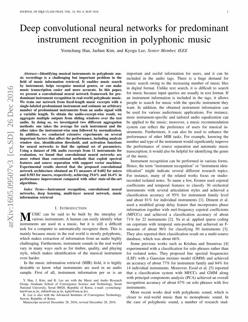
Fig. 1. Schematic of the proposed ConvNet containing 4 times repeated double convolution layers followed by max-pooling. The last max-pooling layerperforms global max-pooling, then it is fed to a fully connected layer followed by 11 sigmoid outputs.

The time-frequency representation of a music signal iscomposed of harmonics from various musical instruments anda human voice. Each musical instrument produces a uniquetimbre with different playing styles, and this type of spectralcharacteristics in music signal might appear in a differentlocation in time and frequency as in the image. ConvNetsare usually composed of many convolutional layers, andinserting a pooling layer between convolutional layers allowsthe network to work at different time scales and introducestranslation invariance with robustness against local distortions.These hierarchical network structures of ConvNets are highlysuitable for representing music audio, because music tends topresent a hierarchical structure in time and different featuresof the music might be more salient at different time scales[21].

Hence, although ConvNets have been a more commonlyused technique in image processing, there are an increasingnumber of attempts to apply ConvNets for music signal. Ithas been reported that ConvNet has outperformed previousstate-of-the-art approaches for various MIR tasks such as onsetdetection [22], automatic chord recognition [23], [24], andmusic structure/boundary analysis [25], [26].

An attempt to apply ConvNets for musical instrumentidentification can be found in the recent report from Parket al. [27] and Li et al. [28], although it is still an ongoingwork and is not a predominant instrument recognition method;hence, there are no other instruments but only target instrumentsounds exist. Our research differs from [27] because we dealwith polyphonic music, while their work is based on thestudio recording of single tones. In addition, our researchalso differs from [28] because we use single-label data fortraining and estimate multi-label data, while they used multi-label data from the training phase. Moreover, they focusedon an end-to-end approach, which is promising in that usingraw audio signals makes the system rely less on domainknowledge and preprocessing, but usually it shows a slightlylower performance than using spectral input such as mel-spectrogram in recent papers [29], [30].

III. SYSTEM ARCHITECTURE

A. Audio PreprocessingThe convolutional neural network is one of the representa-

tion learning methods that allow a machine to be fed with raw

data and to automatically discover the representations neededfor classification or detection [10]. However, appropriate pre-processing of input data is still an important issue to improvethe performance of the system.

In the first preprocessing step, the stereo input audio isconverted to mono by taking the mean of the left and rightchannels, and then it is downsampled to 22,050 Hz from theoriginal 44,100 Hz of sampling frequency. This allows us touse frequencies up to 11,025 Hz, the Nyquist frequency, andit is sufficient to cover most of the harmonics generated bymusical instruments while removing noises possibly includedin the frequencies above this range. Moreover, all audios arenormalized by dividing the time-domain signal with its maxi-mum value. Then, this downsampled time-domain waveform isconverted to a time-frequency representation using short-timeFourier transform (STFT) with 1024 samples for the windowsize (approx. 46 ms) and 512 samples of the hop size (approx.23 ms).

Next, the linear frequency scale-obtained spectrogram isconverted to a mel-scale. We use 128 for the number of mel-frequency bins, following the representation learning paperson music annotation by Nam et al. [31] and Hamel et al. [21],which is a reasonable setting that sufficiently preserves theharmonic characteristics of the music while greatly reducingthe dimensionality of the input data. Finally, the magnitude ofthe obtained mel-frequency spectrogram is compressed with anatural logarithm.

B. Network Architecture

ConvNets can be seen as a combination of feature ex-tractor and the classifier. Our ConvNet architecture generallyfollows a popular AlexNet [18] and VGGNet [32] structure,which contains very deep architecture using repeated severalconvolution layers followed by max-pooling, as shown inFigure 1. This method of using smaller receptive window sizeand smaller stride for ConvNet is becoming highly commonespecially in the computer vision field such as in the studyfrom Zeiler and Fergus [33] and Sermanet et al. [34], whichhas shown superior performance in ILSVRC-2013.

Although the general architecture style is similar to that ofother successful ConvNets in the image processing area, theproposed ConvNet is designed according to our input data. We


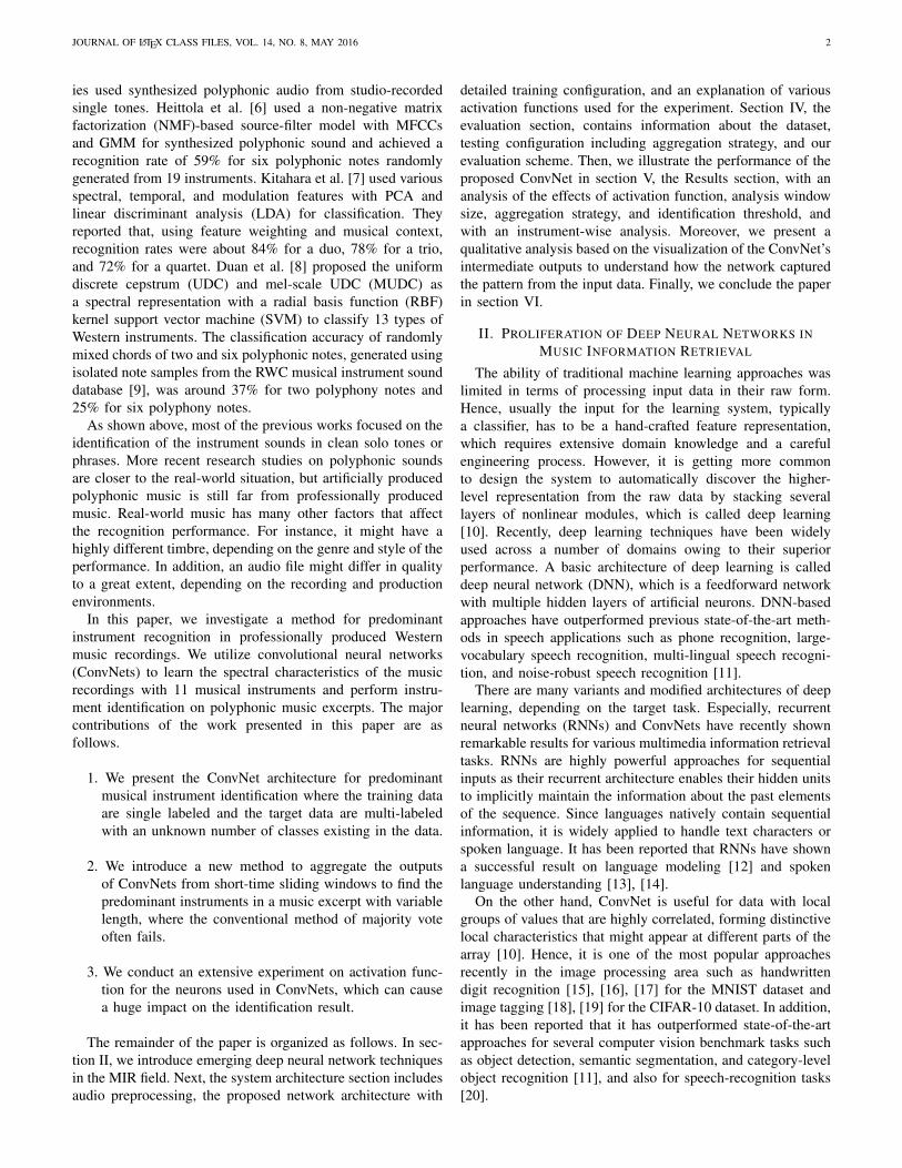
TABLE IPROPOSED CONVNET STRUCTURE. THE INPUT SIZE DEMONSTRATED IN

THIS TABLE IS FOR AN ANALYSIS WINDOW SIZE OF 1 SECOND (NUMBEROF FILTERS × TIME × FREQUENCY). THE ACTIVATION FUNCTION IS

FOLLOWED BY EACH CONVOLUTIONAL LAYER AND A FULLYCONNECTED LAYER. THE INPUT OF EACH CONVOLUTION LAYER IS

ZERO-PADDED WITH 1 × 1, BUT IS NOT SHOWN FOR BREVITY.

Input size Description

1 × 43 × 128 mel-spectrogram32 × 45 × 130 3 × 3 convolution, 32 filters32 × 47 × 132 3 × 3 convolution, 32 filters32 × 15 × 44 3 × 3 max-pooling32 × 15 × 44 dropout (0.25)64 × 17 × 46 3 × 3 convolution, 64 filters64 × 19 × 48 3 × 3 convolution, 64 filters64 × 6 × 16 3 × 3 max-pooling64 × 6 × 16 dropout (0.25)128 × 8 × 18 3 × 3 convolution, 128 filters128 × 10 × 20 3 × 3 convolution, 128 filters128 × 3 × 6 3 × 3 max-pooling128 × 3 × 6 dropout (0.25)256 × 5 × 8 3 × 3 convolution, 256 filters256 × 7 × 10 3 × 3 convolution, 256 filters256 × 1 × 1 global max-pooling1024 flattened and fully connected1024 dropout (0.50)11 sigmoid

use filters with a very small 3× 3 receptive field, with a fixedstride size of 1, and spatial abstraction is done by max-poolingwith a size of 3× 3 and a stride size of 1.

In Table I, we illustrate the detailed ConvNet architecturewith the input size in each layer with parameter values exceptthe zero-padding process. The input for each convolution layeris zero-padded with 1 × 1 to preserve the spatial resolutionregardless of input window size, and we increase the numberof channels for the convolution layer by a factor of 2 afterevery two convolution layers, starting from 32 up to 256.

In the last max-pooling layer after the eight convolutionallayers, we perform global max-pooling followed by one fullyconnected layer. Recently, it has been reported that the use ofglobal average pooling without a fully connected layer beforea classifier layer is less prone to overfitting and shows betterperformance for image processing datasets such as CIFAR-10and MNIST [35]. However, our empirical experiment foundthat global average pooling slightly decreases the performanceand that global max-pooling followed by a fully connectedlayer works better for our task.

Finally, the last classifier layer is the sigmoid layer. Itis common to use a softmax layer when there is only onetarget label, but our system must be able to handle multipleinstruments present at the same time, and, thus, a sigmoidoutput is used.

C. Training Configuration

The training was done by optimizing the categorical cross-entropy between predictions and targets. We used Adam [36]

as an optimizer with a learning rate of 0.001, and the mini-batch size was set to 128. To accelerate the learning processwith parallelization, we used a GTX 970 GPU, which has 4GBof memory.

The training was regularized using dropout with a rate of0.25 after each max-pooling layer. Dropout is a techniquethat prevents the overfitting of units to the training data byrandomly dropping some units from the neural network duringthe training phase [37]. Furthermore, we added dropout aftera fully connected layer as well with a rate of 0.5 since a fullyconnected layer easily suffers from overfitting.

In addition, we conducted an experiment with various timeresolutions to find the optimal analysis size. As our trainingdata were a fixed 3-s audio, we performed the training with3.0, 1.5, 1.0, and 0.5 s by dividing the training audio and usedthe same label for each divided chunk. The audio was dividedwithout overlap for training as it affects the validation lossused for the early stopping. Fifteen percent of the training datawere randomly selected and used as a validation set, and thetraining was stopped when the validation loss did not decreasefor more than two epochs.

The initialization of the network weights is another im-portant issue as it can lead to an unstable learning process,especially for a very deep network. We used a uniformdistribution with zero biases for both convolutional and fullyconnected layers following Glorot and Bengio [38].

D. Activation FunctionThe activation function is followed by each convolutional

layer and fully connected layer. In this section, we introduceseveral activation functions used in the experiment for thecomparison.

The traditional way to model the activation of a neuron is byusing a hyperbolic tangent (tanh) or sigmoid function. How-ever, non-saturating nonlinearities such as the rectified linearunit (ReLU) allow much faster learning than these saturatingnonlinearities, particularly for models that are trained on largedatasets [18]. Moreover, a number of works have shown thatthe performance of ReLU is better than that of sigmoid andtanh activation [39]. Thus, most of the modern studies onConvNets use ReLU to model the output of the neurons [28],[32], [33], [34].

ReLU was first introduced by Nair and Hinton in their workon restricted Boltzmann machines [40]. The ReLU activationfunction is defined as

yi = max(0, zi) (1)

where zi is the input of the ith channel. ReLU simplysuppresses the whole negative part to zero while retainingthe positive part. Recently, there have been several modifiedversions of ReLU introduced to improve the performancefurther. First, leaky-ReLU (LReLU), introduced by Mass etal. [41], compresses the negative part rather than make it allzero, which might cause some initially inactive units to remaininactive. It is defined as

yi =

{zi zi ≥ 0αzi zi < 0

(2)


where α is a parameter between 0 and 1 to give a small gradi-ent in the negative part. Second, parametric ReLU (PReLU),introduced by He et al. [42], is basically similar to LReLUin that it compresses the negative part. However, PReLUautomatically learns the parameter for the negative gradient,unlike LReLU. It is defined as

yi =

{zi zi ≥ 0αizi zi < 0

(3)

where αi is the learned parameters for the ith channel.The choice of activation function considerably influences

the identification performance. It is difficult to say whichspecific activation function always performs the best becauseit highly depends on the parameter setting and the input data.For instance, an empirical evaluation of the ConvNet activationfunctions from Xu et al. [43] reported that the performanceof LReLU is better than those of ReLU and PReLU, butsometimes it is worse than that of basic ReLU, depending onthe dataset and the value for α. Moreover, most of the worksregarding activation function are on the image classificationtask, not on the audio processing domain.

Hence, we empirically evaluated several activation functionsexplained above such as tanh, ReLU, LReLU, and PReLU tofind the most suitable activation function for our task. ForLReLU, very leaky ReLU (α = 0.33) and normal leaky ReLU(α = 0.01) were used, because it has been reported that theperformance of LReLU considerably differs depending on thevalue and that very leaky ReLU works better [43].

We used separate test audio data from the IRMAS dataset,which were not used for the training. First, a sliding windowwas used to analyze the input test audio, which was of thesame size as the analysis window in the training phase. Thehop size of the sliding window was set to half of the windowsize. Then, we aggregated the sigmoid outputs from the slidingwindows by summing all outputs class-wise to obtain a totalamount of activation for each instrument. These 11 summedsigmoid activations were then normalized to be in a rangebetween 0 and 1 by dividing all with the maximum activation.

IV. EVALUATION

A. IRMAS Dataset

The IRMAS dataset includes musical audio excerpts withannotations of the predominant instruments present and isintended to be used for the automatic identification of thepredominant instruments in the music. This dataset was usedin the paper on predominant instrument classification by Boschet al. [44] and includes music from various decades from thepast century, hence differing in audio quality to a great extent.In addition, the dataset covers a wide variability in musical in-strument types, articulations, recording and production styles,and performers.

The dataset is divided into training and testing data, andall audio files are in 16-bit stereo wave with 44,100 Hz ofsampling rate. The training data consisted of 6705 audio fileswith excerpts of 3 s from more than 2000 distinct recordings.Two subjects were paid to obtain the data for 11 pitchedinstruments, as shown in Table II from selected music tracks,

TABLE IILIST OF MUSICAL INSTRUMENTS USED IN THE EXPERIMENT WITH THEIRABBREVIATIONS, AND THE NUMBER OF LABELS OF THE TRAINING AND

TESTING AUDIO.

Instruments Abbreviations Training (n) Testing (n)

Cello cel 388 111Clarinet cla 505 62Flute flu 451 163Acoustic guitar acg 637 535Electric guitar elg 760 942Organ org 682 361Piano pia 721 995Saxophone sax 626 326Trumpet tru 577 167Violin vio 580 211Voice voi 778 1044

with the objective of extracting music excerpts that contain acontinuous presence of a single predominant instrument.

On the other hand, the testing data consisted of 2874 audiofiles with lengths between 5 s and 20 s, and no tracks fromthe training data were included. Unlike the training data,the testing data contained one or more predominant targetinstruments. Hence, the total number of training labels wasidentical to the number of audio files, but the number of testinglabels was more than the number of testing audio files as thelatter are multi-label. For both the training and the testingdataset, other musical instruments such as percussion and basswere not included in the annotation even if they exist in themusic excerpts.

B. Testing Configuration

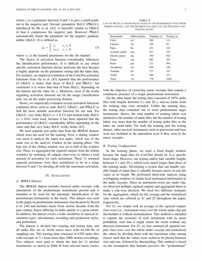
In the training phase, we used a fixed length windowbecause the input data for ConvNet should be in a specificfixed shape. However, our testing audios had variable lengthsbetween 5 s and 20 s, which were much longer than those ofthe training audio. Developing a system that can handle vari-able length of input data is valuable because music in real lifevaries in its length. We performed short-time analysis usingoverlapping windows to obtain local instrument information inthe audio excerpts. Since an annotation exists per audio clip,we observed multiple sigmoid outputs and aggregated them tomake a clip-wise decision. We tried two different strategiesfor the aggregation, which are the average and the normalizedsum, which are referred as S1 and S2 throughout the paper,respectively.

For S1, we simply took an average of the sigmoid outputsclass-wise (i.e., instrument-wise) over the whole audio clip andthresholded it without normalization. This method is intendedto capture the existence of each instrument with its meanprobability such that it might return the result without anydetected instrument. For S2, we first summed all sigmoid out-puts class-wise over the whole audio excerpt and normalizedthe values by dividing them with the maximum value amongclasses such that the values were scaled to be placed betweenzero and one, followed by thresholding. This method is basedon the assumption that humans perceive the “predominant”


Fig. 2. Schematic of obtaining a multi-label output from a test audio signal.Input audio was analyzed with sliding window, and these multiple sigmoidoutputs were aggregated using two different strategies, S1 and S2, to estimatethe predominant instrument for the testing audio excerpt.

instrument in a more relatively scaled sense such that thestrongest instrument is always detected and the existence ofother instruments is judged by their relative strength comparedto the most activate instrument.

Majority vote, one of the most common choices for anumber of classification tasks, is not used in our system.Majority vote first predicts the classes for each analysis frameand the one with more vote wins. However, using this methodfor our task would result in disregarding accompanimentinstruments, piano for example, because a music signal iscomposed of various musical instruments and usually thesounds are overlapped in time domain, and a presence ofaccompaniments are usually much weaker than that of voiceor lead instruments.

As our target is to identify an arbitrary number of predom-inant instruments in testing data, instruments with aggregatedvalue over the threshold were all considered as predominantinstruments. Using a higher value for the identification thresh-old will lead to better precision, but it will obviously decreasethe recall. On the other hand, a lower threshold will increasethe recall, but will lower the precision. Hence, we tried arange of values for the threshold to find the optimal value forthe F1 measure, which is explained in the next PerformanceEvaluation section.

For S1, values between 0.02 and 0.18 were used, and forS2, values between 0.2 and 0.6 were used as a threshold θ.These threshold values were empirically chosen but set to be awide enough range to find the best performance (i.e., highestF1 measure). The schematic of this aggregation process isillustrated in Figure 2.

C. Performance Evaluation

Following the evaluation method widely used in the instru-ment recognition task, we computed the precision and recall,which are defined as

P =tp

tp+ fp(4)

TABLE IIIEXPERIMENT VARIABLES FOR THE ACTIVATION FUNCTION, SIZE OF THE

ANALYSIS WINDOW, AGGREGATION STRATEGY, AND IDENTIFICATIONTHRESHOLD. DEFAULT SETTINGS ARE INDICATED IN BOLD.

Variables

Activation func. tanh, ReLU, PReLU, LReLU (0.01), LReLU (0.33)analysis win. size 0.5 s, 1.0 s, 1.5 s, 3.0 sAgg. strategy S1 (mean), S2 (sum and normalized)θ (S1) 0.02, 0.04, 0.06, 0.08, 0.10, 0.12, 0.14, 0.16, 0.18θ (S2) 0.20, 0.25, 0.30, 0.35, 0.40, 0.45, 0.50, 0.55, 0.60

R =tp

tp+ fn(5)

where tp is true positive, fp is false positive, and fn is falsenegative. In addition, we used the F1 measure to calculatethe overall performance of the system, which is the harmonicmean between precision and recall:

F1 =2PR

P +R(6)

Since the number of annotations for each class (i.e., 11musical instruments) was not equal, we computed the pre-cision, recall, and F1 measure for both the micro and themacro averages. For the micro averages, we calculated themetrics globally regardless of classes, thus giving more weightto the instrument with a higher number of appearances. Onthe other hand, we calculated the metrics for each label andfound their unweighted average for the macro averages; hence,it is not related to the number of instances, but represents theoverall performance over all classes. Finally, we repeated eachexperiment three times and calculated the mean and standarddeviation of the output.

V. RESULTS

We used LReLU (α = 0.33) for the activation function, 1s for the analysis window, S2 for the aggregation strategy,and 0.50 for the identification threshold as default settingsof the experiment where possible, which showed the bestperformance. The experiment variables are listed in Table III.

First, we compared the performance of the proposed Con-vNet with that of the existing algorithm on the IRMAS dataset.The effect of activation function, analysis window, aggregationstrategy, and identification threshold on the recognition perfor-mance was analyzed separately in the following subsections.

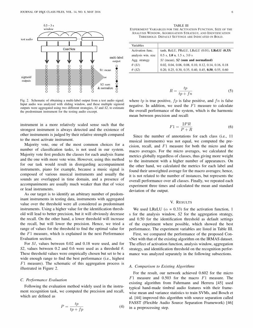
A. Comparison to Existing Algorithms

For the result, our network achieved 0.602 for the microF1 measure and 0.503 for the macro F1 measure. Theexisting algorithm from Fuhrmann and Herrera [45] usedtypical hand-made timbral audio features with their frame-wise mean and variance statistics to train SVMs, and Bosch etal. [44] improved this algorithm with source separation calledFASST (Flexible Audio Source Separation Framework) [46]in a preprocessing step.


Prec. Rec.Micro

F1 Prec. Rec.Macro

F10.0

0.1

0.2

0.3

0.4

0.5

0.6

0.7

0.8Fuhrmann

Bosch

Proposed

Fig. 3. Performance comparison of the predominant instrument recognitionalgorithm from Fuhrmann and Herrra [45], Bosch et al. [44], and our proposedConvNet.

In terms of precision, Fuhrmann and Herrera’s algorithmshowed the best performance for both the micro and themacro measure. However, its recall was very low, around0.25, which resulted in a low F1 measure. Our proposedConvNet architecture outperformed existing algorithms on theIRMAS dataset for both the micro and the macro F1 measure,as shown in Figure 3. From this result, it can be observedthat the learned feature from the input data that is classifiedthrough ConvNet works better than the conventional hand-crafted features with SVMs.

B. Effect of Activation FunctionIn the case of using rectified units as an activation function,

it was possible to observe a significant performance improve-ment compared to the tanh baseline as expected, as shownin Table IV. Unlike the result presented in the ImageNetclassification work from He et al. [42], PReLU did not showany performance improvement, but just showed a matchingperformance with ReLU in our task. On the other hand, usingLReLU showed better performance than using normal ReLUand PReLU. While using LReLU with a small gradient (α= 0.01) showed similar performance to ReLU as expected,LReLU with a very leaky alpha setting (α = 0.33) showed thebest identification performance, which matched the result ofthe empirical evaluation work on ConvNet activation functionfrom Xu et al. [43].

This result shows that suppressing the negative part of theactivation rather than making it all zero certainly improves theperformance compared to normal ReLU because making thewhole negative part zero might cause some initially inactiveunits to be never active as mentioned above. Moreover, thisresult shows that using leaky ReLU, which has been provedto work well in the image classification task, also benefits themusical instrument identification.

0.2 0.25 0.3 0.35 0.4 0.45 0.5 0.55 0.60.52

0.54

0.56

0.58

0.60

0.62

F1-m

easu

re

micro F1-measure

0.5s 1.0s 1.5s 3.0s

0.2 0.25 0.3 0.35 0.4 0.45 0.5 0.55 0.6identification threshold

0.43

0.44

0.45

0.46

0.47

0.48

0.49

0.50

0.51

F1-m

easu

re

macro F1-measure

Fig. 4. Micro and macro F1 measure of an analysis window size of 0.5, 1.0,1.5, and 3.0 s according to the identification threshold.

TABLE IVINSTRUMENT RECOGNITION PERFORMANCE OF THE PROPOSED

CONVNET WITH VARIOUS ACTIVATION FUNCTIONS.

Activation func.Micro Macro

P R F1 P R F1

tanh 0.416 0.625 0.499 0.348 0.537 0.399ReLU 0.640 0.550 0.591 0.521 0.508 0.486PReLU 0.612 0.565 0.588 0.502 0.516 0.490LReLU (α=0.01) 0.640 0.552 0.593 0.530 0.507 0.492LReLU (α=0.33) 0.655 0.557 0.602 0.541 0.508 0.503

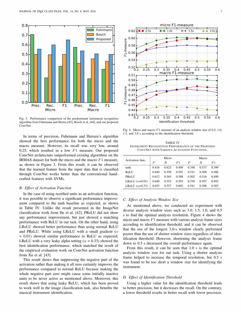
C. Effect of Analysis Window Size

As mentioned above, we conducted an experiment withdiverse analysis window sizes such as 3.0, 1.5, 1.0, and 0.5s to find the optimal analysis resolution. Figure 4 shows themicro and macro F1 measure with various analysis frame sizesaccording to identification threshold, and it can be observedthat the use of the longest 3.0-s window clearly performedpoorer than the use of shorter window sizes regardless of iden-tification threshold. However, shortening the analysis framedown to 0.5 s decreased the overall performance again.

From this result, it can be seen that 1.0 s is the optimalanalysis window size for our task. Using a shorter analysisframe helped to increase the temporal resolution, but 0.5 swas found to be too short a window size for identifying theinstrument.

D. Effect of Identification Threshold

Using a higher value for the identification threshold leadsto better precision, but it decreases the recall. On the contrary,a lower threshold results in better recall with lower precision.


cel cla flu acg elg org pia sax tru vio voi0.0

0.2

0.4

0.6

0.8

1.0F1-m

easure

Optimal setting

Agg. strategy S2 to S1

Analysis win. 1s to 3s

Identification thr. 0.50 to 0.20

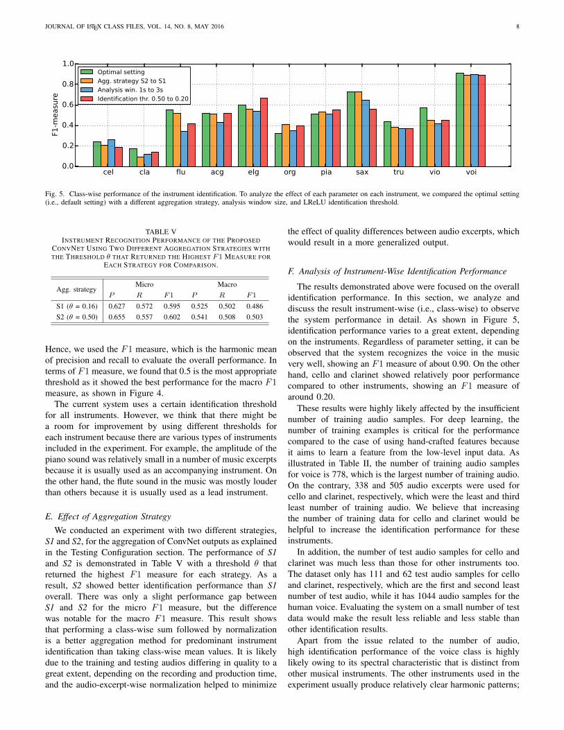
Fig. 5. Class-wise performance of the instrument identification. To analyze the effect of each parameter on each instrument, we compared the optimal setting(i.e., default setting) with a different aggregation strategy, analysis window size, and LReLU identification threshold.

TABLE VINSTRUMENT RECOGNITION PERFORMANCE OF THE PROPOSED

CONVNET USING TWO DIFFERENT AGGREGATION STRATEGIES WITHTHE THRESHOLD θ THAT RETURNED THE HIGHEST F1 MEASURE FOR

EACH STRATEGY FOR COMPARISON.

Agg. strategyMicro Macro

P R F1 P R F1

S1 (θ = 0.16) 0.627 0.572 0.595 0.525 0.502 0.486S2 (θ = 0.50) 0.655 0.557 0.602 0.541 0.508 0.503

Hence, we used the F1 measure, which is the harmonic meanof precision and recall to evaluate the overall performance. Interms of F1 measure, we found that 0.5 is the most appropriatethreshold as it showed the best performance for the macro F1measure, as shown in Figure 4.

The current system uses a certain identification thresholdfor all instruments. However, we think that there might bea room for improvement by using different thresholds foreach instrument because there are various types of instrumentsincluded in the experiment. For example, the amplitude of thepiano sound was relatively small in a number of music excerptsbecause it is usually used as an accompanying instrument. Onthe other hand, the flute sound in the music was mostly louderthan others because it is usually used as a lead instrument.

E. Effect of Aggregation Strategy

We conducted an experiment with two different strategies,S1 and S2, for the aggregation of ConvNet outputs as explainedin the Testing Configuration section. The performance of S1and S2 is demonstrated in Table V with a threshold θ thatreturned the highest F1 measure for each strategy. As aresult, S2 showed better identification performance than S1overall. There was only a slight performance gap betweenS1 and S2 for the micro F1 measure, but the differencewas notable for the macro F1 measure. This result showsthat performing a class-wise sum followed by normalizationis a better aggregation method for predominant instrumentidentification than taking class-wise mean values. It is likelydue to the training and testing audios differing in quality to agreat extent, depending on the recording and production time,and the audio-excerpt-wise normalization helped to minimize

the effect of quality differences between audio excerpts, whichwould result in a more generalized output.

F. Analysis of Instrument-Wise Identification Performance

The results demonstrated above were focused on the overallidentification performance. In this section, we analyze anddiscuss the result instrument-wise (i.e., class-wise) to observethe system performance in detail. As shown in Figure 5,identification performance varies to a great extent, dependingon the instruments. Regardless of parameter setting, it can beobserved that the system recognizes the voice in the musicvery well, showing an F1 measure of about 0.90. On the otherhand, cello and clarinet showed relatively poor performancecompared to other instruments, showing an F1 measure ofaround 0.20.

These results were highly likely affected by the insufficientnumber of training audio samples. For deep learning, thenumber of training examples is critical for the performancecompared to the case of using hand-crafted features becauseit aims to learn a feature from the low-level input data. Asillustrated in Table II, the number of training audio samplesfor voice is 778, which is the largest number of training audio.On the contrary, 338 and 505 audio excerpts were used forcello and clarinet, respectively, which were the least and thirdleast number of training audio. We believe that increasingthe number of training data for cello and clarinet would behelpful to increase the identification performance for theseinstruments.

In addition, the number of test audio samples for cello andclarinet was much less than those for other instruments too.The dataset only has 111 and 62 test audio samples for celloand clarinet, respectively, which are the first and second leastnumber of test audio, while it has 1044 audio samples for thehuman voice. Evaluating the system on a small number of testdata would make the result less reliable and less stable thanother identification results.

Apart from the issue related to the number of audio,high identification performance of the voice class is highlylikely owing to its spectral characteristic that is distinct fromother musical instruments. The other instruments used in theexperiment usually produce relatively clear harmonic patterns;


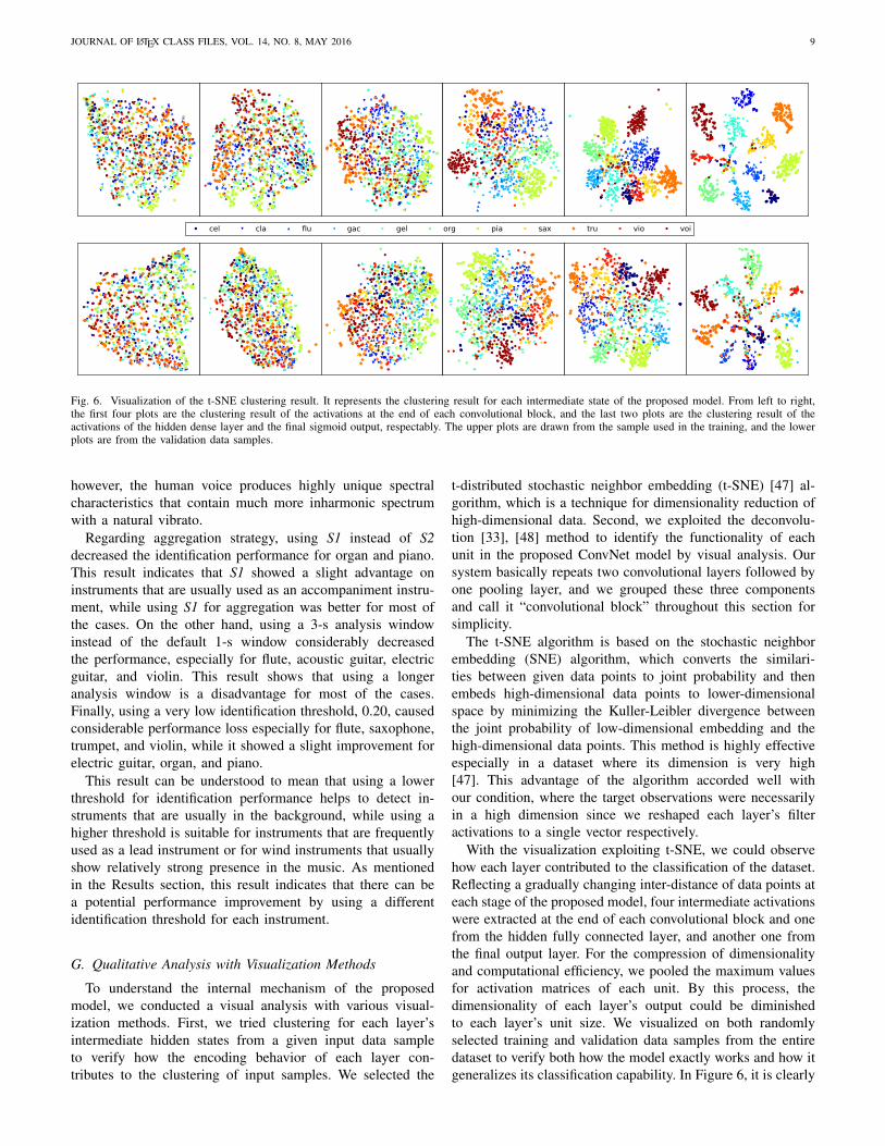
cel cla flu gac gel org pia sax tru vio voi

Fig. 6. Visualization of the t-SNE clustering result. It represents the clustering result for each intermediate state of the proposed model. From left to right,the first four plots are the clustering result of the activations at the end of each convolutional block, and the last two plots are the clustering result of theactivations of the hidden dense layer and the final sigmoid output, respectably. The upper plots are drawn from the sample used in the training, and the lowerplots are from the validation data samples.

however, the human voice produces highly unique spectralcharacteristics that contain much more inharmonic spectrumwith a natural vibrato.

Regarding aggregation strategy, using S1 instead of S2decreased the identification performance for organ and piano.This result indicates that S1 showed a slight advantage oninstruments that are usually used as an accompaniment instru-ment, while using S1 for aggregation was better for most ofthe cases. On the other hand, using a 3-s analysis windowinstead of the default 1-s window considerably decreasedthe performance, especially for flute, acoustic guitar, electricguitar, and violin. This result shows that using a longeranalysis window is a disadvantage for most of the cases.Finally, using a very low identification threshold, 0.20, causedconsiderable performance loss especially for flute, saxophone,trumpet, and violin, while it showed a slight improvement forelectric guitar, organ, and piano.

This result can be understood to mean that using a lowerthreshold for identification performance helps to detect in-struments that are usually in the background, while using ahigher threshold is suitable for instruments that are frequentlyused as a lead instrument or for wind instruments that usuallyshow relatively strong presence in the music. As mentionedin the Results section, this result indicates that there can bea potential performance improvement by using a differentidentification threshold for each instrument.

G. Qualitative Analysis with Visualization Methods

To understand the internal mechanism of the proposedmodel, we conducted a visual analysis with various visual-ization methods. First, we tried clustering for each layer’sintermediate hidden states from a given input data sampleto verify how the encoding behavior of each layer con-tributes to the clustering of input samples. We selected the

t-distributed stochastic neighbor embedding (t-SNE) [47] al-gorithm, which is a technique for dimensionality reduction ofhigh-dimensional data. Second, we exploited the deconvolu-tion [33], [48] method to identify the functionality of eachunit in the proposed ConvNet model by visual analysis. Oursystem basically repeats two convolutional layers followed byone pooling layer, and we grouped these three componentsand call it “convolutional block” throughout this section forsimplicity.

The t-SNE algorithm is based on the stochastic neighborembedding (SNE) algorithm, which converts the similari-ties between given data points to joint probability and thenembeds high-dimensional data points to lower-dimensionalspace by minimizing the Kuller-Leibler divergence betweenthe joint probability of low-dimensional embedding and thehigh-dimensional data points. This method is highly effectiveespecially in a dataset where its dimension is very high[47]. This advantage of the algorithm accorded well withour condition, where the target observations were necessarilyin a high dimension since we reshaped each layer’s filteractivations to a single vector respectively.

With the visualization exploiting t-SNE, we could observehow each layer contributed to the classification of the dataset.Reflecting a gradually changing inter-distance of data points ateach stage of the proposed model, four intermediate activationswere extracted at the end of each convolutional block and onefrom the hidden fully connected layer, and another one fromthe final output layer. For the compression of dimensionalityand computational efficiency, we pooled the maximum valuesfor activation matrices of each unit. By this process, thedimensionality of each layer’s output could be diminishedto each layer’s unit size. We visualized on both randomlyselected training and validation data samples from the entiredataset to verify both how the model exactly works and how itgeneralizes its classification capability. In Figure 6, it is clearly


shown that data samples under the same class of instrumentare well grouped and each group is separated farther, with thelevel of encoding being higher, particularly on the training set.While the clustering was not clearer than the former case, thetendency of clustering on the validation set was also found tobe similar to the training set condition.

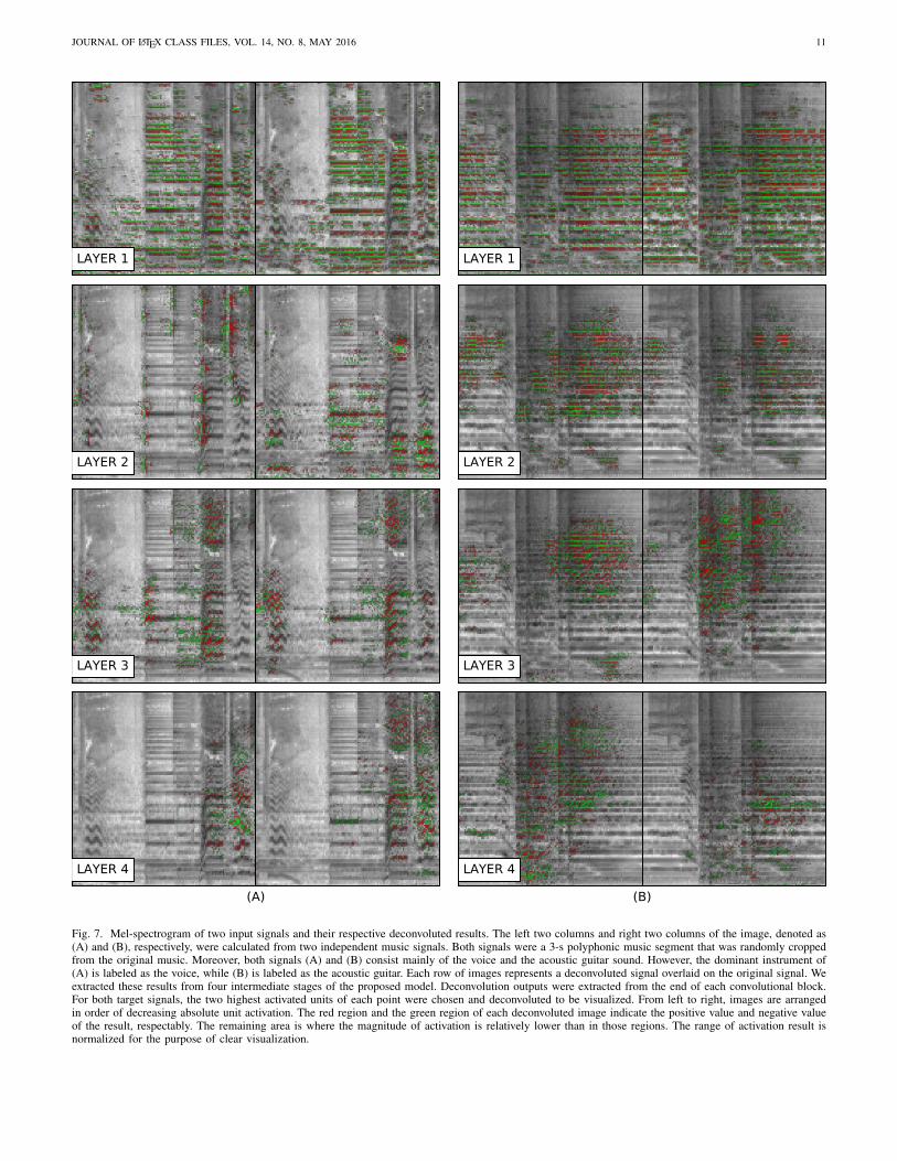
Another visualization method, deconvolution, has recentlybeen introduced as a useful analysis tool to qualitativelyevaluate each node of a ConvNet. The main principle ofthis method is to inverse every stage of operations reachingto the target unit, to generate a visually inspectable imagethat has been, as a consequence, filtered by the trained sub-functionality of the target unit [33]. With this method, it ispossible to reveal intuitively how each internal sub-functionworks within the entire deep convolutional network, whichtends to be thought of as a “black box”.

By this process, the functionality of a sub-part of theproposed model is explored. We generated deconvoluted im-ages like those in Figure 7 from the arbitrary input mel-spectrogram, for each unit in the entire model. From the visualanalysis of the resulting images, we could see several aspectsof the sub-functionalities of the proposed model: (1) Mostunits in the first layer tend to extract vertical, horizontal, anddiagonal edges from the input spectrogram, just like the lowerlayers of ConvNets do in the usual image object recognitiontask. (2) From the second layer through the fourth layer, eachdeconvoluted image indicates that each unit of the mid-layershas a functionality that searches for particular combinations ofthe edges extracted from the first layer. (3) It was found thatit is difficult to strongly declare each sub-part of the proposedmodel that detects a specific musical articulation or expression.However, in an inductive manner, we could see that some unitsindicate that they can be understood as a sub-function of suchmusical expression detector.

We conducted a visual analysis of the deconvoluted imageof two independent music signals, which have the same kindof sound sources, but differently labeled.1 For both cases, themost activated units of the first layer strongly suggested thattheir primary functionality is to detect a harmonic componenton the input mel-spectrogram by finding horizontal edges init, as shown in the top figures in Figure 7. However, fromthe second layer to higher layers, the highly activated units’behavior appeared to be quite different for each respectiveinput signal. For instance, the most activated unit of signal(A)’s second layer showed a functionality similar to onsetdetection, by detecting a combination of vertical and horizontaledges. Compared to this unit, the most activated units ofthe third layer showed a different functionality that seems toactivate unstable components such as the vibrato articulationor the “slur” of the singing voice part, by detecting a particularcombination of diagonal and horizontal edges. On the otherhand, the model’s behavior in signal (B) was very different.As is clearly shown in the second and the third layers’ outputin Figure 7, the highly activated sub-functions were tryingto detect a dense field of stable, horizontal edges which are

1Both signals were composed of a “voice” and an “acoustic guitar”instrument, but the predominant instrument of signal (A) was labeled as the“voice,” while (B) was labeled as the “acoustic guitar”.

often found in harmonic instruments like guitar. Each fielddetected from those units corresponded to the region wherethe strumming acoustic guitar sound is.

VI. CONCLUSION

In this paper, we described how to apply ConvNet to identifypredominant instrument in the real-world music. We trainedthe network using fixed-length single-labeled data, and identifyan arbitrary number of the predominant instrument in a musicclip with a variable length.

Our results showed that very deep ConvNet is capable ofachieving good performance by learning the appropriate fea-ture automatically from the input data. Our proposed ConvNetarchitecture outperformed previous state-of-the-art approachesin a predominant instrument identification task on the IRMASdataset. Mel-spectrogram was used as an input to the ConvNet,and we did not use any source separation in the preprocessingunlike in existing works.

We conducted several experiments with various activationfunctions for ConvNet. Tanh and ReLU were used as a base-line, and the recently introduced LReLU and PReLU were alsoevaluated. Results confirmed that ReLU worked reasonablywell, which is a de facto standard in recent ConvNet studies.Furthermore, we obtained the better results with LReLU thanwith normal ReLU, especially with the very leaky setting (α= 0.33). The performance of Tanh was worse than those ofother rectifier functions as expected, and PReLU just showeda matching performance with ReLU for our task.

This paper also investigated different aggregation methodsfor ConvNet outputs that can be applied to music excerptswith various lengths. We experimented with two different ag-gregation methods, which are the class-wise mean probabilityS2 and the class-wise sum followed by normalization S2. Theexperimental results showed that S2 is a better aggregationmethod because it effectively deals with the quality differencebetween audios through the audio-excerpt-wise normalizationprocess. In addition, we conducted an extensive experimentwith various analysis window sizes and identification thresh-olds. For the analysis window size, using a shorter windowimproved the performance by increasing the temporal reso-lution. However, 0.5 s was too short to obtain an accurateidentification performance, and 1.0 s was found to be theoptimal window size. There was a trade-off between precisionand recall, depending on the identification threshold; hence, weused an F1 measure, which is the harmonic mean of precisionand recall. For the result, a threshold value of 0.5 showed thebest performance.

Visualization of the intermediate outputs using t-SNEshowed that the feature representation became clearer eachtime the input data were passed through the convolutionalblocks. Moreover, visualization using deconvolution showedthat the lower layer tended to capture the horizontal andvertical edges, and that the higher layer tended to seek thecombination of these edges to describe the spectral character-istics of the instruments.

Our study shows that many recent advances in a neuralnetwork on the image processing area are transferable to the


(A) (B)

LAYER 1 LAYER 1

LAYER 2 LAYER 2

LAYER 3 LAYER 3

LAYER 4 LAYER 4

Fig. 7. Mel-spectrogram of two input signals and their respective deconvoluted results. The left two columns and right two columns of the image, denoted as(A) and (B), respectively, were calculated from two independent music signals. Both signals were a 3-s polyphonic music segment that was randomly croppedfrom the original music. Moreover, both signals (A) and (B) consist mainly of the voice and the acoustic guitar sound. However, the dominant instrument of(A) is labeled as the voice, while (B) is labeled as the acoustic guitar. Each row of images represents a deconvoluted signal overlaid on the original signal. Weextracted these results from four intermediate stages of the proposed model. Deconvolution outputs were extracted from the end of each convolutional block.For both target signals, the two highest activated units of each point were chosen and deconvoluted to be visualized. From left to right, images are arrangedin order of decreasing absolute unit activation. The red region and the green region of each deconvoluted image indicate the positive value and negative valueof the result, respectably. The remaining area is where the magnitude of activation is relatively lower than in those regions. The range of activation result isnormalized for the purpose of clear visualization.


audio processing domain. However, audio signal processing,especially music signal processing, has many different aspectscompared to the image processing area where ConvNets aremost extensively used. For example, spectral characteristicsare usually overlapped in both time and frequency unlike theobjects in an image, which makes the detection difficult. More-over, music signals are much more repetitive and continuouscompared to natural images and are present in various lengths.We believe that applying more musical knowledge on the ag-gregation part with adaptive thresholding for each instrumentcan improve the performance further, which warrants deeperinvestigation.

ACKNOWLEDGMENT

This research was supported partly by the MSIP (Ministryof Science, ICT and Future Planning), Korea, under the ITRC(Information Technology Research Center) support program(IITP-2016-H8501-16-1016) supervised by the IITP (Institutefor Information & communications Technology Promotion),and partly by a National Research Foundation of Korea (NRF)grant funded by the MSIP (NRF-2014R1A2A2A04002619).

REFERENCES

[1] A. Eronen and A. Klapuri, “Musical instrument recognition using cep-stral coefficients and temporal features,” in Acoustics, Speech, and SignalProcessing, 2000. ICASSP’00. Proceedings. 2000 IEEE InternationalConference on, vol. 2. IEEE, 2000, pp. II753–II756.

[2] A. Diment, P. Rajan, T. Heittola, and T. Virtanen, “Modified groupdelay feature for musical instrument recognition,” in 10th InternationalSymposium on Computer Music Multidisciplinary Research (CMMR).Marseille, France, 2013.

[3] L.-F. Yu, L. Su, and Y.-H. Yang, “Sparse cepstral codes and powerscale for instrument identification,” in Acoustics, Speech and SignalProcessing (ICASSP), 2014 IEEE International Conference on. IEEE,2014, pp. 7460–7464.

[4] A. Krishna and T. V. Sreenivas, “Music instrument recognition: fromisolated notes to solo phrases,” in Acoustics, Speech, and Signal Process-ing, 2004. Proceedings.(ICASSP’04). IEEE International Conference on,vol. 4. IEEE, 2004, pp. iv–265.

[5] S. Essid, G. Richard, and B. David, “Musical instrument recognitionon solo performances,” in Signal Processing Conference, 2004 12thEuropean. IEEE, 2004, pp. 1289–1292.

[6] T. Heittola, A. Klapuri, and T. Virtanen, “Musical instrument recognitionin polyphonic audio using source-filter model for sound separation.” inISMIR, 2009, pp. 327–332.

[7] T. Kitahara, M. Goto, K. Komatani, T. Ogata, and H. G. Okuno,“Instrument identification in polyphonic music: Feature weighting tominimize influence of sound overlaps,” EURASIP Journal on AppliedSignal Processing, vol. 2007, no. 1, pp. 155–155, 2007.

[8] Z. Duan, B. Pardo, and L. Daudet, “A novel cepstral representation fortimbre modeling of sound sources in polyphonic mixtures,” in Acoustics,Speech and Signal Processing (ICASSP), 2014 IEEE InternationalConference on. IEEE, 2014, pp. 7495–7499.

[9] M. Goto, H. Hashiguchi, T. Nishimura, and R. Oka, “Rwc musicdatabase: Music genre database and musical instrument sound database.”in ISMIR, vol. 3, 2003, pp. 229–230.

[10] Y. LeCun, Y. Bengio, and G. Hinton, “Deep learning,” Nature, vol. 521,no. 7553, pp. 436–444, 2015.

[11] L. Deng and D. Yu, “Deep learning: Methods and applications,” Foun-dations and Trends in Signal Processing, vol. 7, no. 3–4, pp. 197–387,2014.

[12] T. Mikolov, M. Karafiat, L. Burget, J. Cernocky, and S. Khudanpur,“Recurrent neural network based language model.” in INTERSPEECH,vol. 2, 2010, p. 3.

[13] G. Mesnil, X. He, L. Deng, and Y. Bengio, “Investigation of recurrent-neural-network architectures and learning methods for spoken languageunderstanding.” in INTERSPEECH, 2013, pp. 3771–3775.

[14] K. Yao, G. Zweig, M.-Y. Hwang, Y. Shi, and D. Yu, “Recurrent neuralnetworks for language understanding.” in INTERSPEECH, 2013, pp.2524–2528.

[15] Y. LeCun, L. Jackel, L. Bottou, C. Cortes, J. S. Denker, H. Drucker,I. Guyon, U. Muller, E. Sackinger, P. Simard et al., “Learning algorithmsfor classification: A comparison on handwritten digit recognition,”Neural networks: the statistical mechanics perspective, vol. 261, p. 276,1995.

[16] A. Calderon, S. Roa, and J. Victorino, “Handwritten digit recognitionusing convolutional neural networks and gabor filters,” Proc. Int. Congr.Comput. Intell, 2003.

[17] X.-X. Niu and C. Y. Suen, “A novel hybrid cnn–svm classifier forrecognizing handwritten digits,” Pattern Recognition, vol. 45, no. 4, pp.1318–1325, 2012.

[18] A. Krizhevsky, I. Sutskever, and G. E. Hinton, “Imagenet classificationwith deep convolutional neural networks,” in Advances in neural infor-mation processing systems, 2012, pp. 1097–1105.

[19] J. Ngiam, Z. Chen, D. Chia, P. W. Koh, Q. V. Le, and A. Y. Ng, “Tiledconvolutional neural networks,” in Advances in Neural InformationProcessing Systems, 2010, pp. 1279–1287.

[20] G. Hinton, L. Deng, D. Yu, G. E. Dahl, A.-r. Mohamed, N. Jaitly,A. Senior, V. Vanhoucke, P. Nguyen, T. N. Sainath et al., “Deep neuralnetworks for acoustic modeling in speech recognition: The shared viewsof four research groups,” Signal Processing Magazine, IEEE, vol. 29,no. 6, pp. 82–97, 2012.

[21] P. Hamel, S. Lemieux, Y. Bengio, and D. Eck, “Temporal poolingand multiscale learning for automatic annotation and ranking of musicaudio.” in ISMIR, 2011, pp. 729–734.

[22] J. Schluter and S. Bock, “Improved musical onset detection with convo-lutional neural networks,” in Acoustics, Speech and Signal Processing(ICASSP), 2014 IEEE International Conference on. IEEE, 2014, pp.6979–6983.

[23] E. J. Humphrey and J. P. Bello, “Rethinking automatic chord recog-nition with convolutional neural networks,” in Machine Learning andApplications (ICMLA), 2012 11th International Conference on, vol. 2.IEEE, 2012, pp. 357–362.

[24] N. Boulanger-Lewandowski, Y. Bengio, and P. Vincent, “Audio chordrecognition with recurrent neural networks.” in ISMIR, 2013, pp. 335–340.

[25] K. Ullrich, J. Schluter, and T. Grill, “Boundary detection in musicstructure analysis using convolutional neural networks.” in ISMIR, 2014,pp. 417–422.

[26] T. Grill and J. Schluter, “Music boundary detection using neural net-works on combined features and two-level annotations,” in Proceedingsof the 16th International Society for Music Information Retrieval Con-ference (ISMIR 2015), Malaga, Spain, 2015.

[27] T. Park and T. Lee, “Musical instrument sound classification with deepconvolutional neural network using feature fusion approach,” arXivpreprint arXiv:1512.07370, 2015.

[28] P. Li, J. Qian, and T. Wang, “Automatic instrument recognition inpolyphonic music using convolutional neural networks,” arXiv preprintarXiv:1511.05520, 2015.

[29] Y. Hoshen, R. J. Weiss, and K. W. Wilson, “Speech acoustic modelingfrom raw multichannel waveforms,” in Acoustics, Speech and SignalProcessing (ICASSP), 2015 IEEE International Conference on. IEEE,2015, pp. 4624–4628.

[30] D. Palaz, R. Collobert, and M. M. Doss, “Estimating phoneme classconditional probabilities from raw speech signal using convolutionalneural networks,” arXiv preprint arXiv:1304.1018, 2013.

[31] J. Nam, J. Herrera, M. Slaney, and J. O. Smith, “Learning sparse featurerepresentations for music annotation and retrieval.” in ISMIR, 2012, pp.565–570.

[32] K. Simonyan and A. Zisserman, “Very deep convolutional networks forlarge-scale image recognition,” arXiv preprint arXiv:1409.1556, 2014.

[33] M. D. Zeiler and R. Fergus, “Visualizing and understanding convolu-tional networks,” in Computer vision–ECCV 2014. Springer, 2014, pp.818–833.

[34] P. Sermanet, D. Eigen, X. Zhang, M. Mathieu, R. Fergus, and Y. Le-Cun, “Overfeat: Integrated recognition, localization and detection usingconvolutional networks,” arXiv preprint arXiv:1312.6229, 2013.

[35] M. Lin, Q. Chen, and S. Yan, “Network in network,” arXiv preprintarXiv:1312.4400, 2013.

[36] D. Kingma and J. Ba, “Adam: A method for stochastic optimization,”arXiv preprint arXiv:1412.6980, 2014.

[37] N. Srivastava, G. Hinton, A. Krizhevsky, I. Sutskever, and R. Salakhut-dinov, “Dropout: A simple way to prevent neural networks from over-


fitting,” The Journal of Machine Learning Research, vol. 15, no. 1, pp.1929–1958, 2014.

[38] X. Glorot and Y. Bengio, “Understanding the difficulty of training deepfeedforward neural networks,” in International conference on artificialintelligence and statistics, 2010, pp. 249–256.

[39] J. Gu, Z. Wang, J. Kuen, L. Ma, A. Shahroudy, B. Shuai, T. Liu,X. Wang, and G. Wang, “Recent advances in convolutional neuralnetworks,” arXiv preprint arXiv:1512.07108, 2015.

[40] V. Nair and G. E. Hinton, “Rectified linear units improve restricted boltz-mann machines,” in Proceedings of the 27th International Conferenceon Machine Learning (ICML-10), 2010, pp. 807–814.

[41] A. L. Maas, A. Y. Hannun, and A. Y. Ng, “Rectifier nonlinearitiesimprove neural network acoustic models,” in Proc. ICML, vol. 30, 2013,p. 1.

[42] K. He, X. Zhang, S. Ren, and J. Sun, “Delving deep into rectifiers:Surpassing human-level performance on imagenet classification,” inProceedings of the IEEE International Conference on Computer Vision,2015, pp. 1026–1034.

[43] B. Xu, N. Wang, T. Chen, and M. Li, “Empirical evaluation of rectifiedactivations in convolutional network,” arXiv preprint arXiv:1505.00853,2015.

[44] J. J. Bosch, J. Janer, F. Fuhrmann, and P. Herrera, “A comparison ofsound segregation techniques for predominant instrument recognition inmusical audio signals.” in ISMIR, 2012, pp. 559–564.

[45] F. Fuhrmann and P. Herrera, “Polyphonic instrument recognition for ex-ploring semantic similarities in music,” in Proc. of 13th Int. Conferenceon Digital Audio Effects DAFx10, 2010, pp. 1–8.

[46] N. Ono, K. Miyamoto, H. Kameoka, J. Le Roux, Y. Uchiyama,E. Tsunoo, T. Nishimoto, and S. Sagayama, “Harmonic and percussivesound separation and its application to mir-related tasks,” in Advancesin music information retrieval. Springer, 2010, pp. 213–236.

[47] L. Van der Maaten and G. Hinton, “Visualizing data using t-sne,” Journalof Machine Learning Research, vol. 9, no. 2579-2605, p. 85, 2008.

[48] J. Yosinski, J. Clune, A. Nguyen, T. Fuchs, and H. Lipson, “Under-standing neural networks through deep visualization,” arXiv preprintarXiv:1506.06579, 2015.

Yoonchang Han was born in Seoul, Republic ofKorea, in 1986. He studied electronic engineeringsystems at King’s College London, UK, from 2006to 2009, and then moved to Queen Mary Universityof London, UK, and received an MEng (Hons)degree in digital audio and music system engineeringwith First Class Honours in 2011. He is currently aPhD candidate in digital contents and informationstudies at the Music and Audio Research Group(MARG), Seoul National University, Republic ofKorea. His main research interest lies within devel-

oping deep learning techniques for automatic musical instrument recognition.

Jaehun Kim was born in Seoul, Republic of Korea,in 1986. He is currently a researcher at the Musicand Audio Research Group. His research interestsinclude signal processing and machine learning tech-niques applied to music and audio. He received aBA in English literature and linguistics from SeoulNational University and received an MS degree inthe digital contents and information studies at theMusic and Audio Research Group (MARG), SeoulNational University, Republic of Korea.

Kyogu Lee is an associate professor at Seoul Na-tional University and leads the Music and AudioResearch Group. His research focuses on signalprocessing and machine learning techniques appliedto music and audio. Lee received a PhD in computer-based music theory and acoustics from StanfordUniversity.

journal of la deep convolutional neural networks for ... · deep convolutional neural networks for...

Documents