C

RB

KSa

b

c

d

e

h

•••••

a

ARRA

KEfCMI

1

fdr2a

U

0h

Journal of Neuroscience Methods 219 (2013) 205– 219

Contents lists available at ScienceDirect

Journal of Neuroscience Methods

jou rn al hom epage: www.elsev ier .com/ locate / jneumeth

omputational Neuroscience

eproducible paired sources from concurrent EEG-fMRI data usingICAR

evin S. Browna,b,c,d,∗, Ryan Kaspere,b, Barry Giesbrechte,b, Jean M. Carlsona,b,cott T. Graftone,b

Department of Physics, University of California, Santa Barbara, CA 93106, USAInstitute for Collaborative Biotechnologies, University of California, Santa Barbara, CA 93106, USAChemical and Biomolecular Engineering, University of Connecticut, Storrs, CT 06269, USADepartment of Marine Sciences, University of Connecticut, Groton, CT 06340, USADepartment of Psychological and Brain Sciences, University of California, Santa Barbara, CA 93106, USA

i g h l i g h t s

We introduce BICAR, a new algorithm for subject-level EEG-fMRI data fusion.BICAR ranks each joint source by a task-independent measure of reproducibility.We derive an analytical reproducibility cutoff below which components are discarded.We apply BICAR to human subjects performing a visual search task.Among the most reproducible sources are visual, motor, and attentional components.

r t i c l e i n f o

rticle history:eceived 11 March 2013eceived in revised form 22 July 2013ccepted 22 July 2013

eywords:EGMRI

a b s t r a c t

We introduce BICAR, an algorithm for obtaining robust, reproducible pairs of temporal and spatial com-ponents at the individual subject level from concurrent electroencephalographic and functional magneticresonance imaging data. BICAR assigns a task-independent measure of component quality, reproducibil-ity, to each paired source. Under BICAR a reproducibility cutoff is derived that can be used to objectivelydiscard spuriously paired EEG-fMRI components. BICAR is run on minimally processed data: fMRI imagesundergo the standard preprocessing steps (alignment, motion correction, etc.) and EEG data, after scan-ner artifact removal, are simply bandpass filtered. This minimal processing allows the secondary scoring

oncurrent EEG-fMRIultimodal data fusion

ndependent component analysis

of the same set of BICAR components for a variety of different endpoint analyses; in this manuscriptwe propose a general method for scoring components for task event synchronization (evoked responseanalysis), but scoring using many other criteria, for example frequency content, are possible. BICAR isapplied to five subjects performing a visual search task, and among the most reproducible componentswe find biologically relevant paired sources involved in visual processing, motor planning, execution,and attention.

. Introduction

Concurrent surface electroencephalography and whole-brainunctional magnetic resonance imaging (EEG-fMRI) hold tremen-ous promise for obtaining non-invasive high spatiotemporal

esolution measurements of human brain dynamics (Debener et al.,006). Multiple studies support the idea that EEG sources and fMRIctivations in healthy subjects can colocalize (Christmann et al.,

∗ Corresponding author at: 1080 Shennecossett Road, Groton, CT 06340-6040,SA. Tel.: +1 860 405 9136.

E-mail address: kevin.s.brown@uconn.edu (K.S. Brown).

165-0270/$ – see front matter © 2013 Elsevier B.V. All rights reserved.ttp://dx.doi.org/10.1016/j.jneumeth.2013.07.012

© 2013 Elsevier B.V. All rights reserved.

2007; Whittingstall et al., 2007; Roberts et al., 2008; Esposito et al.,2009; Dubois et al., 2012; Logothetis et al., 2001). In addition, incertain patient populations, especially epileptics being consideredfor surgical therapy, EEG-fMRI is emerging as a promising alter-native to invasive corticography (Rosenkranz and Lemieux, 2010).The most compelling reason for fusing EEG and fMRI is that theyare complementary. Trying to infer the locations of cortical sourcesfrom EEG data alone is a highly underdetermined inverse problemwhich will not yield a unique solution without employing ad hoc

constraints on solution norm or smoothness (Sekihara et al., 2001;Pascual-Marqui et al., 1994; Hämäläinen and Ilmoniemi, 1994).Conversely, even if major advances in pulse-sequence technologycould vastly shorten MRI acquisition times (Lustig et al., 2007;

2 scienc

Cfme

mditiW2ou(Mf2eat

gte1amBtpd

mfieccttpiucobtrhgm

BrptdrBcsfigce

06 K.S. Brown et al. / Journal of Neuro

andès and Wakin, 2008; Jung et al., 2009; Jeromin et al., 2012),MRI is fundamentally a slow metabolic/hemodynamic measure-

ent that cannot yield the kind of time resolution obtainable fromlectrodynamic measurements.

Despite a general belief that EEG-fMRI is better than eithereasurement on its own, general methods for combining these

ata of vastly different spatial and temporal resolution are lack-ng (Chaudhary et al., 2011). Some existing methods make heavyrade-offs for or against spatial or temporal resolution, for examplen the case of fMRI event (Grouiller et al., 2011; Mulert et al., 2002;

u et al., 2010; Yuah et al., 2012) and EEG source (Babiloni et al.,002; Liu et al., 2006; Strobel et al., 2008) weighting. Other meth-ds build specialized solutions geared towards obtaining a solutionseful for analysis in frequency space, as is the case for waveletsSchultze-Kraft et al., 2011) or partial least squares (Martinez-

ontes et al., 2004). A variety of other methods based on responseunctions (Sato et al., 2010), mutual information (Ostwald et al.,010, 2012), or variational Bayesian approximations (Daunizeaut al., 2007) have been proposed, but typically time locking to

behavioral event of interest is essential for obtaining a solu-ion.

Joint estimations aim to take a symmetric approach to inte-rating EEG-fMRI data sets; the most straightforward way to dohis is with Independent Component Analysis (ICA) (Moosmannt al., 2008). EEG is modeled using temporal ICA (Makeig et al.,996) and fMRI via spatial ICA (McKeown et al., 1998). Thesepproaches have the advantage of requiring no source localizationodel, though one could be used if desired (Brookings et al., 2009;

rown et al., 2010). Joint estimations typically have the disadvan-age of relying heavily on the task structure and/or rather arbitraryrocessing/reshaping of the data matrices to obtain conformableimensions across subjects or modalities.

It is extremely challenging to establish reliable and unbiasedethods to match ICA components systematically. This is a dif-

cult problem even when considering a single imaging modality,.g. selection of spatial fMRI sources alone. One solution is to matchomponents at a population level by finding components that areonsistent across subjects (Eichele et al., 2008). However, in ordero be diagnostically important, a solution must be obtainable athe individual subject level. Another promising approach to theroblem of unbiased component selection for single data modal-

ties is given by the RAICAR algorithm (Yang et al., 2008), whichses a repeated estimations technique to assess the robustness ofomponents. Each component is given a task-independent measuref component quality: the reproducibility. This value is calculatedy performing stochastic ICA many times on the same dataset andhen matching components across realizations. Components whichepeatedly occur in many realizations are more reproducible andence more trustworthy. However, RAICAR is limited to use on sin-le modalities and therefore not suitable for joint EEG-fMRI dataining.Motivated by the strategy of RAICAR, we recently developed

ICAR: a general-purpose data-driven method for obtaining robust,eproducible pairs of temporal and spatial components from com-lementary spatiotemporal data matrices (Brown et al., 2012). Inhat paper the algorithm is applied to many different types of data,emonstrating the general applicability of BICAR for spatiotempo-al data fusion. In this manuscript, the extension and application ofICAR to event-related analysis of EEG-fMRI data as a specific appli-ation is introduced. To apply BICAR to EEG-fMRI data, a number ofignificant modifications and improvements were necessary. BICARollows RAICAR (Yang et al., 2008) in assigning an experiment-

ndependent measure of component quality (reproducibility), butoes beyond RAICAR in several ways, most notably in the appli-ation to joint EEG-fMRI data. BICAR has five key advantages overxisting methods applied to this problem:

e Methods 219 (2013) 205– 219

Objectivity: In BICAR one can analytically calculate a data- andalgorithm-dependent reproducibility cutoff below which a sub-ject’s components should be deemed insignificant; this cutoff isderived in this manuscript. This entirely removes the subjectivitythat accompanies many ICA analyses, in which components areselected by eye using prior anatomical or task information.Flexibility: Only scanner acquisition times and data sampling ratesare used in BICAR; no information about the task or paradigm isrequired. BICAR is run on the preprocessed data, with no epoching,calculation of t-maps, etc. This allows the same set of BICARcomponents to be used for multiple endpoint analyses: evokedresponses, frequency content, spatial priors, etc. This is a crucialpoint; while we consider event-related analysis in this manuscript,that choice is made after BICAR is run on the data. BICAR itselfremains completely ignorant of the task events in the experiment.Extensibility: BICAR is not a source localization method, but resultsfrom BICAR could be directly used in source localization studies:highly reproducible components could be used as basis functionsin a joint inversion approach (Brookings et al., 2009; Brown et al.,2010).Specificity: BICAR produces joint components at the individualsubject level. This allows the discovery of both subject-commonand subject-unique dynamics, which could be important forunderstanding behavioral variability (Miller et al., 2002, 2011).Methods like group ICA (Calhoun et al., 2001) which begin atthe population level only reveal activity common to the entirepopulation.Symmetry: Unlike event or source weighting methods, BICARtreats the two data sources on identical footing by taking thebest resolved dimension of each: time from EEG and space fromfMRI. In addition, it is possible to adjust the relative weightingbetween the two data sources to accentuate temporal or spatialinformation.

In what follows, the BICAR algorithm is discussed in the contextof application to EEG-fMRI data (see Section 2). Full details on thealgorithm and its performance on a variety of test data are avail-able elsewhere (Brown et al., 2012). Here we introduce for the firsttime a general method for scoring BICAR components for significantassociation with task events; this allows selection of BICAR com-ponents which are both reproducible and significantly associatedwith a set of task events of interest.

Not only can BICAR assign a reproducibility value to eachjoint source, but it is also possible to calculate a reproducibil-ity cutoff below which BICAR components are deemed to bespuriously paired and should be ignored. This derivation isdiscussed in detail in this manuscript, and is an importantadvance. Simply ranking the components by reproducibility givesone an order for consideration (most reproducible first), butoffers no guidance as to which joint components to neglect forfurther analysis. The reproducibility cutoff provides this guid-ance.

In this manuscript, BICAR is applied to a set of healthy par-ticipants with normal attention performing a visual search task.BICAR is able to find biologically relevant paired sources involved invisual processing, motor planning, execution, and attention, whichare highly reproducible and present in multiple subjects. In theseexamples, we focus on finding components that are relevant for anevent related experimental design for individual subjects and notto perform a large sample, group analysis. It should be stressed thatthis is only one application. Other scoring criteria, such as frequency

analysis, can be applied to the same set of BICAR components afterthe algorithm is used. BICAR only needs to be repeated if the EEG orfMRI data itself changes, for example because of different choicesin image preprocessing.

K.S. Brown et al. / Journal of Neuroscienc

Fig. 1. Single target-search task used in this study. After presentation of a fixationcross, a field of “L”s is presented along with one rotated “T”, in one of two possibleooi

2

2

2

cEBacpE

2

vG‘lttcitFhrcsmt

ato‘autiw

o

rientations. Subjects search the visual field until they find the “T”, reporting on itsrientation via a button press. Search fields were either from a small item set (sixtems total) or a large item set (twelve items total).

. Methods

.1. Experimental design

.1.1. ParticipantsFive study participants (four female, one male) performed a

hallenging visual search task during a two hour simultaneousEG-fMRI experiment at the University of California, Santa Barbararain Imaging Center. All of them self-reported as right handed,nd ranged in age from 20 to 30 years. All volunteers had normal ororrected-to-normal visual acuity. Prior to participation, volunteersrovided written informed consent that had been approved by thethical Committee of the University of California, Santa Barbara.

.1.2. Task and procedureThe orientation task we used is one that is commonly used in

isual search tasks (Chun and Jiang, 1998; Johnson et al., 2007;iesbrecht et al., 2013). The search field consisted of rotated colored

L’ distractors and a single rotated ‘T’ target (see Fig. 1). The itemocation for each array was randomly sampled from a grid of six-een possible locations with the constraint that across all trials thearget was equally likely to be in any of these locations. Each trialould be either a small set size (six items) or a large set size (twelvetems), as well as either ‘repeated’ (identical array of search itemso one seen previously) or ‘novel’ (random layout of search items).or repeated displays, the distractor locations and identities wereeld constant, but the target was rotated 90◦ to the left or 90◦ to theight (equal numbers of trials). In order to facilitate the contextualueing effect participants were instructed to adopt a passive searchtrategy (Lleras and Von Mühlenen, 2004). For the analysis in thisanuscript, we aggregate across all target presentations and call

hem all “stimuli”.The search task procedure was as follows. Each trial started with

central fixation to be maintained at all times. After 250 ms of fixa-ion, a search array was displayed until either the subject respondedr 1900 ms elapsed. The subject had to indicate whether the target

T’ was rotated to the left or right by pressing one of two buttonss quickly as possible. Responses were made with the right handsing a button box. After response, auditory feedback was giveno indicate whether the answer was correct (high pitched beep) or

ncorrect (buzzer). In this article we discard all incorrect responses

hen studying the “response” category.Each trial lasted a total of three seconds. A total of eight blocks

f trials were used for each subject, with each block consisting

e Methods 219 (2013) 205– 219 207

of eight small and eight large displays repeated twice for a totalof 256 experimental trials. In addition, approximately 85 blanktrials (one third of 256) were included in each block to intro-duce temporal jitter into the paradigm. During the blank trials,no target/distractor field was presented; the fixation cross simplyremained on the screen. Importantly, the orientation of the target(left or right with respect to an upright ‘T’) was completely coun-terbalanced and randomized so that in each block, every display(regardless of whether it was ‘novel’ or ‘repeated’) was presentedtwice, once with the target rotated left and once with the targetrotated right. The ‘repeated’ and ‘novel’ aspects refer only to config-uration of the target and distractor encountered previously. Acrossblocks, new displays consisting of unique target/distractor spatialconfigurations were created for the ‘novel’ condition and the orig-inal configurations from the ‘repeated’ condition were again usedtwice per block, once for each orientation. This counterbalancingand randomization procedure removes any motor biases associ-ated with a particular display and ensures that the task (orientationdiscrimination) is orthogonal to the spatial configuration manipu-lation (‘novel’ vs. ‘repeated’).

In order to avoid removing task-relevant signal from concur-rently recorded EEG during MR artifact correction, the search arraypresentations were not explicitly tied to a TR onset (Allen et al.,2000). Instead, the initial search array was presented following thefirst TR after a random delay. This delay and the three-second triallength avoided regular synchronization with the two second TR.

2.1.3. Data collection and preprocessingAll data was collected at the UCSB Brain Imaging Center.Electroencephalographic data was acquired simultaneously

with fMRI data using an MR-compatible 64 channel EEG system(www.brainproducts.com). Eight five-minute sessions of EEG-fMRIdata were collected for each subject. The data was acquired at1000 Hz and re-referenced offline to an average of electrodesTP9 and TP10 (near mastoids). MR gradient switching artifactswere removed via BrainVision Analyzer software version 2.0(www.brainproducts.com); the correction process creates an arti-fact template for each TR based on scanner triggers, and thistemplate is subtracted from the raw EEG data (Allen et al., 2000).Following this correction, the data was downsampled to 250 Hz.

The ballistocardiogram artifact was removed via Niazy’s OBSmethod (Niazy et al., 2005), using the FMRIB plugin for EEGLab(sccn.ucsb.edu/eeglab). After BCG correction the ECG electrodewas discarded. Each electrode in each imaging session was bandpass filtered between 0.1 and 30 Hz, downsampled to 62.5 Hz, andlinearly detrended before concatenation. This resulted in a two-dimensional array of size number of electrodes (nE) by number ofEEG samples (tE).

A 3T TIM TRIO Siemens Magnetom scanner with a 12-channelphased-array head coil was used for MRI data collection. The func-tional data were acquired using a T2*-weighted gradient-echosequence with a repetition time (TR) of 2 s, echo time (TE) of30 ms, and flip angle (FA) of 90◦, resulting in 56 contiguous slices at3 mm × 3 mm × 3.5 mm voxel resolution. For anatomical data, a T1-weighted MPRAGE sequence with 1 mm isometric voxel resolutionwas used.

fMRI data were preprocessed using SPM 5.0(www.fil.ion.ucl.ac.uk/spm) (Friston et al., 1995). fMRI imagevolumes were slice time corrected, motion corrected, unwarped,spatially normalized to the Montreal 152 Average T1 atlas, andresliced to 4 mm × 4 mm × 4 mm voxel sizes. No smoothing wasperformed on the fMRI images. Each voxel in each imaging session

was linearly detrended and the sessions were concatenated; thesesteps occurred after all SPM preprocessing steps. The high resolu-tion T1 anatomical MRI was segmented into gray and white matter,warped to the 152 T1 atlas, and resliced to 4 mm × 4 mm × 4 mm

208 K.S. Brown et al. / Journal of Neuroscience Methods 219 (2013) 205– 219

Fig. 2. Schematic for the BICAR algorithm. BICAR proceeds first by K-fold FastICA decomposition of the EEG and fMRI data matrices E and B ; nS is the number of extracteds RI dys rces, ea associ

vusop

bmajs

2

2

dEFb(mrcdwftstifra

ources. Then sources are paired using a transfer function between the EEG and fMearched and aligned via absolute correlation; this results in nS groups of paired soure then averaged with weighting to obtain one set of nS paired BICAR sources and

oxel sizes. The combined gray and white matter images weresed as masks for each subject to remove non-brain voxels beforeession concatenation and reshaping into a two-dimensional arrayf the number of scans (tF) by the number of voxels (nV). Thisrocess was replicated for all five subjects.

For two of the five subjects, one of the eight sessions had toe discarded as there were errors in the time stamps needed toake a correspondence between the EEG record and fMRI volume

cquisition times within the five-minute session. For these two sub-ects, the other seven sessions were used. For the remaining threeubjects all eight recording sessions were usable.

.2. BICAR

.2.1. AlgorithmThe steps of the BICAR algorithm (Brown et al., 2012) are

iscussed here in order to highlight particulars of applying it toEG-fMRI data. Fig. 2 gives an algorithm schematic. In Fig. 2A K-foldastICA (Hyvärinen and Oja, 1997) decomposition is performed onoth the EEG data matrix (size nE × tE) and the fMRI data matrixsize tF × nV). By K-fold FastICA we mean the following. Each data

atrix (E and B in Fig. 2) is unmixed via FastICA with a differentandom initial condition; we refer to a single pair of FastICAompositions as a realization. The initial unmixing matrix for eachecomposition is a matrix of Gaussian distributed random numbersith mean zero and unit variance of the appropriate size (nE × nS

or E, tF × nS for B). This matrix is orthogonalized in at the start ofhe FastICA algorithm. Temporal ICA is used on the EEG matrix andpatial ICA on the fMRI data matrix; the fMRI data matrix has beenransposed in Fig. 2A so that time (scans) is the row dimension, as

s appropriate for spatial ICA. All initial conditions – both for dif-erent values of K and for spatial and temporal ICA within a singleealization – are independent. K = 30 was used for this study. Bothpplications of ICA in each realization extract nS sources; for all

namics. The cross-realization correlation matrices between the paired sources areach of which consists of one source from each of the K ICA realizations. Componentsated mixing matrices. See Section 2 for details on these steps.

analyses in this paper, nS = 63, representing a full-rank decompo-sition of the EEG data matrix E. Hence in what follows nS = nE = 63in Fig. 2, though this is not generally required (see below foradditional information on this point). Each ICA decomposition foreach dataset produces both nS sources and nS mixing elements. Forthe EEG data, the sources are time series and the mixing elementsare typically called scalp maps. For the fMRI data, the sources areimage volumes and the mixing elements are time series.

After decomposition, EEG sources are matched to the fMRIsources (Fig. 2B). This matching step is performed by pairingtransformed, decimated EEG sources (time series) with fMRI mix-ing elements (also time series) via absolute Pearson correlation.Sources are paired one-to-one. One-to-many matching is also pos-sible, but our previous work has considered only one-to-one sourcematching (Brown et al., 2012). In order to carry out the match-ing step, a transfer function between the EEG and fMRI dynamicsneeds to be specified. We have shown elsewhere via simulationthat BICAR is relatively robust to transfer function misspecification(Brown et al., 2012); in addition, it is possible to optimize the trans-fer function from within BICAR itself, a subject for a future study.For the transfer function a simple parameterized function of thetype often assumed for the hemodynamic response function (HRF)in fMRI research was employed. This is a single non-delayed gammaof the form

h(t, {˛, �}) =(

t

�

)˛ e−t/�

��( ̨ + 1), (1)

which basically acts as a delayed low pass filter. The parametervalues used were ̨ = 8.6, � = 0.55, resulting in a peak location of4.73 s. After transformation by the HRF and before the correla-tion calculations, the transformed EEG sources were decimated

to establish temporal correspondence with the fMRI scans. Cor-relation matching proceeds as follows and occurs independentlyin each realization. The source pair in each realization with thelargest absolute transformed EEG source/fMRI loading correlation

scienc

aTy

T(eoHrrutBertru

p(mstEstasobsm

mItssrtadittamc

wscaiaucweuaaf2

K.S. Brown et al. / Journal of Neuro

re associated and removed from the pool of potential matches.his process is then repeated, in this case 62 additional times, toield nS = 63 paired sources in each of the K = 30 ICA realizations.

The paired sources are then aligned across realizations (Fig. 2C).his process is rather complicated and the details for both RAICARYang et al., 2008) and BICAR (Brown et al., 2012) can be foundlsewhere. The goal can be understood as follows. The orderingf the nS paired sources in each of the K realizations is arbitrary.ence, even if an identical set of paired sources was found in each

ealization, we still must construct a consistent ordering in eachealization so that similar sources can be grouped. Therefore, wese a realization-realization cross-correlation technique in ordero compute an optimal ordering. We then construct each of the nSICAR sources as a weighted average of K sources, one instance fromach of the ordered K realizations, with the weighting factors rep-esenting the averaged pairwise reproducibility of sources acrosshe K estimates. For example, in the case of identical sources in eachealization (rarely achieved in practice), all the weights would benity.

After this process of weighted averaging one BICAR decom-osition has the same shape as two regular ICA decompositionsone temporal, one spatial) concatenated; the BICAR source

atrix will be of dimensions nS × tE + nV (number of extractedources × number of EEG samples + number of fMRI voxels) andhe BICAR mixing matrix of dimensions nE + tF × nS (number ofEG electrodes + number of fMRI scans × number of extractedources). In practice, all the matrices are kept separate for compu-ational efficiency. However, it is useful to think this way becauselignment is driven by both temporal (from EEG sources) andpatial (from fMRI sources) information; highly similar groupsf sources are similar in both time and space. Once BICAR haseen run, the temporal and spatial parts of the BICAR sources areeparated and related to anatomical and other experimental infor-ation.Before source averaging and reproducibility calculation, one

ust deal with a sign problem. In both the EEG and fMRI cases,CA produces a set of sources and mixing elements that reconstructhe corresponding data matrix. However, one can easily change theign of any number of sources along with the signs of the corre-ponding columns of the mixing matrix and the data matrix willemain invariant. Since we have used absolute Pearson correla-ion for similarity calculations, sources in one realization may beligned with their sign-reversed version in another. Hence a proce-ure is employed to fix the signs of each aligned component; this

s accomplished by arbitrarily assigning one source in each groupo have the “canonical” sign, and then computing signed correla-ions of that source with all others in the group. Any source having

negative correlation with the canonical source is multiplied byinus one; the corresponding mixing column also obtains a sign

hange.Once alignment and sign canonicalization are finished the

eighted averages are constructed. For each of the nS aligned BICARources, we compute the K × K set of estimate-estimate absoluteross-correlations. There are K(K − 1)/2 unique such correlations,ccounting for the symmetry of the cross-correlations and ignor-ng autocorrelation. We define the reproducibility of a BICAR sourcend its corresponding mixing elements as the average of thesenique correlations. The weight for each of the K estimates inonstructing the BICAR source is given by the average of the pair-ise absolute cross-correlations of that estimate with all other

stimates. These definitions place reproducibility in [0, 1]. Contrib-tions to the reproducibility come from both time (EEG sources)

nd space (fMRI sources). Matching, sign canonicalization, sourceveraging, and reproducibility are either not present in, or quite dif-erent from, the RAICAR algorithm (Yang et al., 2008; Brown et al.,012).

e Methods 219 (2013) 205– 219 209

The choice of 63 sources – a full-rank decomposition of the EEGdata – is motivated by previous work (Brown et al., 2012). By usingBICAR on synthetic data of known source content, we investigatedthe result of source overextraction from the temporal data. Specifi-cally, ten sources were extracted from a mixture containing onlyfive true sources. In all cases, BICAR source reproducibility wascorrelated with BICAR source similarity to a true source, and thespurious sources migrated to the tail of the reproducibility distri-bution. This was true even in low signal-to-noise scenarios; in fact,in cases of high signal-to-noise the shape of the BICAR source repro-ducibility spectrum (see Fig. 3 for an example) could be used toestimate the number of true sources in the data. In these low noisecases, the sorted reproducibility values drop sharply between thelast true source and the first spurious source (sources five and six inthe synthetic example). Given that we do not know the true numberof sources in the real neuroimaging data, this previous result givesus confidence that overextraction is safer than underextraction, inwhich we might not capture all the true neural sources.

2.2.2. Component displayFigs. 4–6 show BICAR components from the subjects in this

study. Common display conventions for the BICAR components areas follows. In every case, for sources which are significantly task-associated, the temporal portion of the BICAR source is shown asa stacked plot of individual trials (as a raster) and trial average (asa line plot). No information about the temporal source is shownfor nonsynchronized components. For both synchronized and non-synchronized components, representative slices are shown for thespatial sources. More specific information follows:

Temporal: Time windows of extracted signals for the stimulus andresponse categories were (−0.24 s, 0.64 s) and (−0.72 s, 0.24 s),respectively, where the event of interest (search field presenta-tion or button press) occurred at 0 s. For components which aresynchronized to both categories, rasters and event average plotsare shown separately for both event types (stimuli and responses).All extracted windows were baselined using the pre-event inter-val. Each raster has been transformed with a nonlinear (hyperbolictangent) contrast adjustment for easier viewing; this transforma-tion is for visualization only and was not used in calculation ofevent synchronization or the trial means. Shaded gray areas in thetrial average plots are envelopes representing two standard errorsof the mean, and the event onset (t = 0) is marked with a verticaldotted line in each signal average plot. The y-axis units in the sig-nal average plot are arbitrary; each signal has been standardizedbefore display. A colormap in which green is more positive and redmore negative has been employed, but the overall sign of the com-ponent is essentially arbitrary – it is jointly carried by the sourceand the mixing elements (not shown).Spatial: Each spatial source is shown as a series of representa-tive slices, superimposed on that subject’s anatomy. In each figureshowing BICAR components (Figs. 4–6), the set of slices is alwaysthe same. They are numbers 35, 38, 41, 44, and 47. This is notedon the first BICAR source in each figure (top left); the numberingis suppressed elsewhere due to space constraints. BICAR spatialsources have been standardized before display. All spatial sourceshave been smoothed with an isotropic Gaussian filter with a half-width of 4 mm (1 voxel); as detailed in Experimental Design, nosmoothing was performed on the fMRI images themselves. In addi-tion, voxels with absolute intensity less than a chosen threshold

of 0.25 have been suppressed. The same red/green colormap usedfor the temporal rasters has been used for the spatial sources,but again the sign of the component is essentially arbitrary – it isjointly carried by the source and the mixing elements (not shown).

210 K.S. Brown et al. / Journal of Neuroscience Methods 219 (2013) 205– 219

Fig. 3. Sample reproducibility spectrum with schematics for scoring. BICAR itself, via physical matching, gives each resulting component a reproducibility value (the y-axisin the central plot). The dotted line shows a sample reproducibility cutoff Rc , whose derivation is given in Section 3 and Appendix A. Filling the symbols in the central plotindicates significant task-association with one or both categories (all Stimuli, all Responses, or Both), with category indicated by color. Significance for task association isd tions

t al det

2

wcsesBetatfa

s

wtcr

it(Fmm

a

etermined by comparing intertrial similarity when epoching to the real event locaime by a uniform random number in (−500 ms, 500 ms). See Section 3 for addition

.3. Ranking components for task-relevance

BICAR run on each subject produces nS joint components, eachith an associated reproducibility value R ∈ [0, 1]. The components

an then be secondarily scored on other criteria of interest. In thistudy only secondary scoring for phase synchronization to taskvents (i.e., evoked response analysis) is considered. Scores for taskynchronization are obtained as follows. The EEG portion of theICAR component is epoched separately with respect to each taskvent category of interest; for the analysis in this paper there arewo categories of interest, all stimuli (search field presentations)nd correct responses. The Ni trials from each category i are usedo compute average inter-trial similarities for each component asollows. Computing the Ni × Ni correlation matrix C(i), we compute

synchronization index for component c and category i

c(i) = 1Ni(Ni − 1)

∑k /= l

C2kl(i) (2)

hich sums the squares of the unique trial-to-trial cross correla-ions. The sum is restricted to off-diagonal terms, and the prefactororrects for double counting the upper triangle and its counterparteflected across the diagonal.

In this study each component has two values for s, correspond-ng to the categories chosen for analysis.1 To determine whetherhese synchronization values are statistically significant, s in Eq.2) is recomputed for sets of permuted stimuli in each category.

or each category (all stimuli, all correct responses) a set of per-uted task events is created in which the true trigger locations areoved in time by uniform random numbers in (−500 ms, 500 ms).

1 There are two categories of interest in this study, but this process generalizes tony number of categories.

versus a distribution of scrambled locations, in which each real trigger is moved inails on these calculations.

These jitter times will be experiment-dependent, but the scoringmethod is not. These permuted trigger sets preserve the numberof stimuli but onsets are shifted with respect to the true valuesin the experiment. For each permuted task sc(i) is recomputed forall components c. This process is replicated 100 times to obtain acategory-specific distribution for sc(i). This distribution is then usedto standardize the observed true s values, and the resulting stan-dardized scores converted to p-values. A false discovery rate (FDR)correction (Benjamini and Hochberg, 1995) is applied to accountfor multiple hypothesis testing, and the calculated p-values com-pared to the FDR-corrected cutoffs for significance. In general, atthe end of this process each component will be significantly asso-ciated with zero or more categories: for the subsequent analysisin this manuscript, that means stimuli, responses, both, or neither.The p-value threshold was 0.05 (corrected).

It should be emphasized here that this secondary scoring hasa lot to do with how the experiment was performed and whatquantities are of biological interest; for example, evoked versusspontaneous activity, correct or incorrect responses, etc. However,reproducibility is assessed in a completely task-independent man-ner; many different secondary analyses of interest can be appliedto BICAR components, and none of them affect the BICAR decom-position.

3. Results

3.1. Reproducibility cutoff

BICAR ranks each paired component by reproducibility but by

itself does not generate a significance level below which an indi-vidual subject’s components are deemed to be spuriously pairedduring the matching step. Such an approximate cutoff can be ana-lytically derived, and it is dependent on both the data and BICAR’s

K.S. Brown et al. / Journal of Neuroscience Methods 219 (2013) 205– 219 211

Fig. 4. Most reproducible stimulus-synchronized BICAR components. This figure and Figs. 5 and 6 show the four most reproducible BICAR components from each of the fivesubjects in this study. The portion of those twenty components that are significantly synchronized to either stimuli alone (blue box) or both stimuli and responses (blackbox) are shown here. The colors of the enclosing boxes have been chosen to match the point colors in Fig. 8 and give the task event association. All signals and slices ares r the

s he texs

pbo

pEariti

R

Hp[dfc

w(fr

hown as described in Section 2. Slice numbering in the spatial sources is shown folices. Component numbering (in boxes) is arbitrary and used for easy reference in tame as in Fig. 8.

arameters. More details on this derivation are given in Appendix A,ut here we introduce the ideas behind, and summarize the resultsf, those calculations.

Consider a “worst-case” random, nondegenerate componentairing: if two individually reproducible components – one fromEG and one from fMRI – were paired spuriously, one could obtainn artificially highly reproducible BICAR component that does notepresent a true joint component. Suppose there is a componentn the EEG data which has reproducibility R* close to unity; thenhe reproducibility R of a BICAR component whose spatial portions randomly paired with this temporal source is

= wR∗ + (1 − w)

⎡⎣ 2

K(K − 1)

∑i,j;j>i

rij

⎤⎦ . (3)

ere, w is the weight given to the EEG data — all calculations in thisaper use w = 1/2, but in deriving the cutoff we simply require w ∈0, 1]. rij is the absolute correlation between two spatial sources inifferent realizations. All BICAR sources consist of one componentrom each of K realizations, hence there will be K(K − 1)/2 uniqueorrelations to sum.

Calculating R in Eq. (3) therefore depends critically on what

e will call the (spatial) RAICAR distribution, after Yang et al.

2008). Fig. 7A shows a sample RAICAR distribution from realMRI data. Note the logarithmic scale on the y axis; most cross-ealization absolute correlations are small. Considering random,

first source but suppressed thereafter; all spatial sources have the same displayedt. Subject number (S1, S2, etc.) is included to the left of each component, and is the

nondegenerate pairing means that to calculate R one drawsK(K − 1)/2 random rijs from the RAICAR distribution and computestheir mean. This then means that the reproducibility of randompairs depends on the data and algorithm parameters via the statis-tics of the RAICAR distribution.

The rij are certainly identically distributed, and if not completelyindependent very nearly so. For even moderate K the sum in Eq. (3)can have hundreds of terms. The central limit theorem thus givesthe distribution for the term in brackets as:

2K(K − 1)

∑rij∼N

(〈rij〉,

2�2(rij)K(K − 1)

), (4)

where N(�, �2) is a normally distributed random number withmean � and variance �2, and 〈rij〉 and �2(rij) are the mean andvariance of the spatial RAICAR distribution, respectively. Since thesum is normally distributed, the spurious reproducibility R is alsonormally distributed as

R∼N

(wR∗ + (1 − w)〈rij〉, (1 − w)2 2�2(rij)

K(K − 1)

), (5)

a normal variate with

〈R〉 = wR∗ + (1 − w)〈rij〉 (6)

�(R) =√

2(1 − w)�(rij)√K(K − 1)

. (7)

212 K.S. Brown et al. / Journal of Neuroscience Methods 219 (2013) 205– 219

Fig. 5. Most reproducible response-synchronized BICAR components. The portion of the four most reproducible BICAR components from each of the five subjects which aresignificantly synchronized to responses. Component numbering continues that begun in Fig. 4. Slices, signals, and subject number are shown as described in Section 2 andthe caption of Fig. 4.

K.S. Brown et al. / Journal of Neuroscience Methods 219 (2013) 205– 219 213

F the pt and ia

s

R

ari

Fliu

ig. 6. Most reproducible nonsynchronized BICAR components. This figure showsask-associated. The component numbering here continues the numbering in Fig. 5nd 5.

This spurious reproducibility distribution can be used to set aignificance bound. Specifically, set the bound Rc as

c = 〈R〉 + n��(R), (8)

desired n� standard deviations above the expected spuriouseproducibility. Note that as K → ∞ , Rc → 〈R〉. The reproducibil-ty cutoffs calculated in this study use w = 1/2 and n� = 2. If we

ig. 7. Sample RAICAR distributions. (A) A sample real spatial RAICAR distribution for

ogarithmic scale; the vast majority of the cross-realization absolute correlations in real

n Appendix A. For 63 extracted sources, the ratio of the density at ε to that at 1.0 is appnimportant in either case and both distributions have been rescaled for legibility.

ortion of the twenty BICAR components which were not found to be significantlys used for easy reference in the main text. Slice numbering is the same as in Figs. 4

further assume the most reproducible component in the EEG datahas R* = 1, then

Rc = 1 + 〈rij〉2

+√

2K(K − 1)

�(rij) (9)

fMRI data, with a smoothed estimated of the histogram shown in red. Note thedata are small. (B) Idealized RAICAR distribution used in the analytical calculationroximately 8.3. The scale in this figure is also logarithmic; the actual y values are

2 scienc

Ofc

•

•

••

iatafatosbEtvrR

3

teddvdtpae

fiiatfitSBhtsapRag

14 K.S. Brown et al. / Journal of Neuro

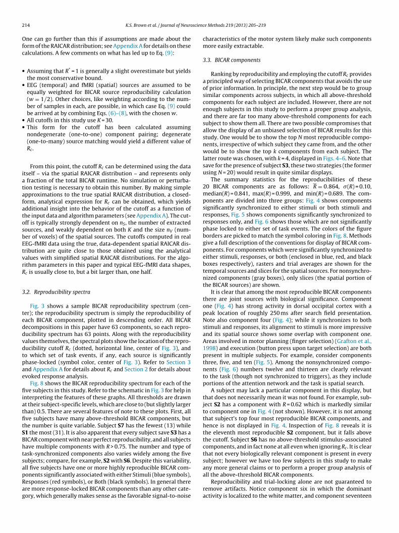
ne can go further than this if assumptions are made about theorm of the RAICAR distribution; see Appendix A for details on thesealculations. A few comments on what has led up to Eq. (9):

Assuming that R* = 1 is generally a slight overestimate but yieldsthe most conservative bound.EEG (temporal) and fMRI (spatial) sources are assumed to beequally weighted for BICAR source reproducibility calculation(w = 1/2). Other choices, like weighting according to the num-ber of samples in each, are possible, in which case Eq. (9) couldbe arrived at by combining Eqs. (6)–(8), with the chosen w.All cutoffs in this study use K = 30.This form for the cutoff has been calculated assumingnondegenerate (one-to-one) component pairing; degenerate(one-to-many) source matching would yield a different value ofRc.

From this point, the cutoff Rc can be determined using the datatself – via the spatial RAICAR distribution – and represents only

fraction of the total BICAR runtime. No simulation or perturba-ion testing is necessary to obtain this number. By making simplepproximations to the true spatial RAICAR distribution, a closed-orm, analytical expression for Rc can be obtained, which yieldsdditional insight into the behavior of the cutoff as a function ofhe input data and algorithm parameters (see Appendix A). The cut-ff is typically strongly dependent on nS, the number of extractedources, and weakly dependent on both K and the size nV (num-er of voxels) of the spatial sources. The cutoffs computed in realEG-fMRI data using the true, data-dependent spatial RAICAR dis-ribution are quite close to those obtained using the analyticalalues with simplified spatial RAICAR distributions. For the algo-ithm parameters in this paper and typical EEG-fMRI data shapes,c is usually close to, but a bit larger than, one half.

.2. Reproducibility spectra

Fig. 3 shows a sample BICAR reproducibility spectrum (cen-er); the reproducibility spectrum is simply the reproducibility ofach BICAR component, plotted in descending order. All BICARecompositions in this paper have 63 components, so each repro-ucibility spectrum has 63 points. Along with the reproducibilityalues themselves, the spectral plots show the location of the repro-ucibility cutoff Rc (dotted, horizontal line, center of Fig. 3), ando which set of task events, if any, each source is significantlyhase-locked (symbol color, center of Fig. 3). Refer to Section 3nd Appendix A for details about Rc and Section 2 for details aboutvoked response analysis.

Fig. 8 shows the BICAR reproducibility spectrum for each of theve subjects in this study. Refer to the schematic in Fig. 3 for help in

nterpreting the features of these graphs. All thresholds are drawnt their subject-specific levels, which are close to (but slightly largerhan) 0.5. There are several features of note to these plots. First, allve subjects have many above-threshold BICAR components, buthe number is quite variable. Subject S7 has the fewest (13) while1 the most (31). It is also apparent that every subject save S3 has aICAR component with near perfect reproducibility, and all subjectsave multiple components with R > 0.75. The number and type ofask-synchronized components also varies widely among the fiveubjects; compare, for example, S2 with S6. Despite this variability,ll five subjects have one or more highly reproducible BICAR com-

onents significantly associated with either Stimuli (blue symbols),esponses (red symbols), or Both (black symbols). In general therere more response-locked BICAR components than any other cate-ory, which generally makes sense as the favorable signal-to-noise

e Methods 219 (2013) 205– 219

characteristics of the motor system likely make such componentsmore easily extractable.

3.3. BICAR components

Ranking by reproducibility and employing the cutoff Rc providesa principled way of selecting BICAR components that avoids the useof prior information. In principle, the next step would be to groupsimilar components across subjects, in which all above-thresholdcomponents for each subject are included. However, there are notenough subjects in this study to perform a proper group analysis,and there are far too many above-threshold components for eachsubject to show them all. There are two possible compromises thatallow the display of an unbiased selection of BICAR results for thisstudy. One would be to show the top N most reproducible compo-nents, irrespective of which subject they came from, and the otherwould be to show the top k components from each subject. Thelatter route was chosen, with k = 4, displayed in Figs. 4–6. Note thatsave for the presence of subject S3, these two strategies (the formerusing N = 20) would result in quite similar displays.

The summary statistics for the reproducibilities of these20 BICAR components are as follows: R = 0.864, �(R) = 0.10,median(R) = 0.841, max(R) = 0.999, and min(R) = 0.689. The com-ponents are divided into three groups: Fig. 4 shows componentssignificantly synchronized to either stimuli or both stimuli andresponses, Fig. 5 shows components significantly synchronized toresponses only, and Fig. 6 shows those which are not significantlyphase locked to either set of task events. The colors of the figureborders are picked to match the symbol coloring in Fig. 8. Methodsgive a full description of the conventions for display of BICAR com-ponents. For components which were significantly synchronized toeither stimuli, responses, or both (enclosed in blue, red, and blackboxes respectively), rasters and trial averages are shown for thetemporal sources and slices for the spatial sources. For nonsynchro-nized components (gray boxes), only slices (the spatial portion ofthe BICAR sources) are shown.

It is clear that among the most reproducible BICAR componentsthere are joint sources with biological significance. Componentone (Fig. 4) has strong activity in dorsal occipital cortex with apeak location of roughly 250 ms after search field presentation.Note also component four (Fig. 4); while it synchronizes to bothstimuli and responses, its alignment to stimuli is more impressiveand its spatial source shows some overlap with component one.Areas involved in motor planning (finger selection) (Grafton et al.,1998) and execution (button press upon target selection) are bothpresent in multiple subjects. For example, consider componentsthree, five, and ten (Fig. 5). Among the nonsynchronized compo-nents (Fig. 6) numbers twelve and thirteen are clearly relevantto the task (though not synchronized to triggers), as they includeportions of the attention network and the task is spatial search.

A subject may lack a particular component in this display, butthat does not necessarily mean it was not found. For example, sub-ject S2 has a component with R = 0.62 which is markedly similarto component one in Fig. 4 (not shown). However, it is not amongthat subject’s top four most reproducible BICAR components, andhence is not displayed in Fig. 4. Inspection of Fig. 8 reveals it isthe eleventh most reproducible S2 component, but it falls abovethe cutoff. Subject S6 has no above-threshold stimulus-associatedcomponents, and in fact none at all even when ignoring Rc. It is clearthat not every biologically relevant component is present in everysubject; however we have too few subjects in this study to makeany more general claims or to perform a proper group analysis of

all the above-threshold BICAR components.

Reproducibility and trial-locking alone are not guaranteed toremove artifacts. Notice component six in which the dominantactivity is localized to the white matter, and component seventeen

K.S. Brown et al. / Journal of Neuroscience Methods 219 (2013) 205– 219 215

R

R

R

Source Nu mber

S1 S2

S3 S6

S7

F ematc ble cod ntly t

trehwccsbbaeSKVda

ig. 8. Reproducibility spectra for the five subjects in this study. Fig. 3 gives a schalculations used to assess significance. Note that the number of highly reproduciotted horizontal line) varies among the five subjects, as do the number of significa

hat is at least partially a vascular artifact. Artifacts can also beeproducible! They can also be significantly phase-locked to taskvents, as for example susceptibility artifacts induced by a verticalead movement coincident with each button press or stimulus;hile this particular artifact is not among the most reproducible

omponents shown here, it is present as an above-thresholdomponent in subject S1 (not shown). Artifacts with stereotypicalpatial or temporal patterns, in either EEG or fMRI, could be foundy using a secondary scoring method that selects componentsased on similarity to temporal or spatial templates. Alternatively,n artifact correction (not trial-based rejection) method could bemployed before running BICAR. This was not done in this study.ince many correction methods are ICA-based (Jung et al., 2000;

lados et al., 2011; Wallstrom et al., 2004; Urrestarazu et al., 2004;igário, 1997), if this route were chosen the resulting reduction inata dimensionality after correction would have to be taken intoccount when setting nS in BICAR.

ic guide to understanding the various features of reproducibility spectra and themponents (those which sit above the subject-specific cutoff Rc , represented by a

ask-associated components. Compare, for example, subjects S2 and S6.

4. Discussion

BICAR, a new general algorithm for spatiotemporal data fusionwas applied to concurrent EEG-fMRI data. The utility of the algo-rithm has been shown at the individual subject level of analysisusing five participants who performed a spatial search task. Aprocedure was described to obtain a data-dependent significancecutoff for BICAR components, as well as a simple method to analyzeBICAR components post hoc for evidence of statistically signifi-cant phase-locking to task events of interest. Some of the mostreproducible BICAR components are clearly biologically relevant.Components representing visual processing, attention, motor plan-ning, and execution were found in multiple subjects.

The response-locked components are more impressive than thestimulus-locked ones and easier to find; this likely has to do withthe nature of the task. Since the real stimulus-associated cognitiveevent of interest is not associated directly with presentation of the

2 scienc

siitmtoa

T(jIblitaetmt2taiSnr

oartEdpnafraftcapba(

ranmwgI21abaAfa

16 K.S. Brown et al. / Journal of Neuro

earch field, but rather with localizing and discriminating the targettem (Buschman and Miller, 2007), it can be difficult to locate. Thiss because localization and discrimination will occur at a variableime after search field presentation and before the motor response,

aking it poorly trial-aligned with either trigger. Nevertheless, forhe purposes of this demonstration, there is a robust identificationf movement and to a lesser degree, visual stimulus synchronizedctivity.

It bears repeating that no task information is used in BICAR itself.his means BICAR could be used in multiple ways, for example:a) to reveal evoked activity, as in this manuscript, (b) to classifyoint components based on frequency information, and (c) as anCA-based pre-filter for removing non-reproducible activity fromoth the EEG and fMRI datasets, which could then be further ana-

yzed using almost any existing EEG-fMRI method. Item (b) aboves an obvious extension: trigger related or global (whole signal)ime-frequency maps could be computed and components rankedccording to power in frequency bands of interest (alpha, beta, mu,tc.). Yet another scoring method potentially relevant for the searchask described in this manuscript would be to analyze the temporal

ixing coefficients – scalp maps – for sterotypical patterns similaro those observed with the P300 event-related potential (Polich,007), and rank them in order of similarity to this pattern. Again,his would not require any reanalysis of the BICAR components,s the data itself has not changed, only the endpoint quantity ofnterest. Multiple secondary scoring methods could also be used.coring of components on any axes other than reproducibility willecessarily reflect the goals of the scientist and the experiment;eproducibility exists outside of these considerations.

There are several ways to improve BICAR, of which two standut: optimization of the transfer function (TF) connecting the EEGnd fMRI data from within BICAR itself, and integration of BICAResults into a population-level analysis. The first of these is impor-ant because, while we expect in general that the TF connecting theEG and fMRI data will resemble an HRF, it is not an HRF. It connectsynamics to dynamics, in the form of transformed, decimated tem-oral sources to mixing matrix elements for spatial sources. BICAReeds a TF to run, and for this study a reasoned guess has been madebout the likely shape of the TF and its parameters. The results evenrom this simple assumption are promising, but there are manyeasons to believe a simple HRF is suboptimal for this problem. Anlgorithm for estimating the TF from within BICAR would benefitrom calibration via simulations, with gains via simulation leadingo direct improvements in real data applications, as TF estimatesloser to the true value will generate better component matchesnd higher component reproducibility. Higher reproducibility com-onents are of higher quality, as (a) low reproducibility is generatedy averaging together groups of components with low similarity,nd (b) our prior simulation studies have demonstrated that trueknown) sources have higher reproducibility (Brown et al., 2012).

While the emphasis of the current work was to establish theeliability of the BICAR method at the individual subject level ofnalysis, additional methods will be needed to combine compo-ents across subjects for group level inference. The most effectiveethod for placing BICAR results in a population-level analysisould likely involve data clustering. Clustering has been used to

ood effect with neuroimaging data, particularly for organizingCA analyses of fMRI data (Himberg et al., 2004; Esposito et al.,005), separating EEG data into microstates (Pascual-Marqui et al.,995), and grouping voxel time series (Goutte et al., 1999). Allbove-threshold BICAR components across all study subjects coulde clustered using a dissimilarity measure in both time (trigger-

ligned averages of temporal sources) and space (image volumes).fter clustering, group-average components could be constructed

rom the clusters, but reproducibility should again be taken intoccount here. Since the reproducibility of above-threshold BICAR

e Methods 219 (2013) 205– 219

components can vary by almost a factor of two (depending upon thevalue of Rc), the group averages should be reproducibility weighted.This allows the most reproducible components to carry the mostweight in the group mean, which is as it should be, since theyrepresent the most well-estimated activity.

One-to-one, nondegenerate matching of temporal and spatialsources was considered exclusively in this manuscript. In somesituations, matching multiple temporal sources to a single spatialsource may be appropriate (Yuah et al., 2012). Many-to-one degen-erate matching is possible in BICAR but would require modificationsto the existing algorithm. For one, the details of reproducibility cut-off calculation would change, though not its motivation and utility.In a situation where not all spatial components survive matchingto be incorporated into BICAR components, to calculate the cut-off we would no longer be sampling from the full spatial RAICARdistribution (Fig. 7) but rather from a restricted distribution of onlythe cross-correlations among the subset of spatial components thatare matched to a temporal component in any realization pair. Thistherefore means that we would have to calculate the cutoff afterthe matching step rather than after decomposition as done here,and the assumptions underlying our analytical calculations wouldno longer hold. However, even in the case of one-to-one match-ing, one could eschew the calculated cutoff we present here andinstead create ensembles of random matches. While this would bemuch more computationally intensive, it would not be prohibitive,would be easily parallelizable, and would pose no additional the-oretical difficulties. Hence one could always default to simulatingthe null model if a suitably accurate calculated cutoff could not bederived.

Another more subtle issue is the allowed degree of degener-acy: how few spatial components would we tolerate? It may bedesirable to reward not only good match quality, in the sense ofhigh correlation between transformed temporal sources and spa-tial loadings, but also to reward diversity of source selection. Thiswould allow retention of more unique spatial components in thematches while sacrificing some total match quality, which would beparticularly desirable if that match quality sacrifice was small com-pared to the number of additional components retained. A balancebetween goodness-of-fit and source inclusion could be obtained bymatching using a multiobjective cost function that rewards highaverage correlation in the matches but penalizes the overall matchset for including fewer unique spatial sources. However, the properweighting of the goodness-of-fit and diversity terms would requiresubstantial investigation. In addition, the use of a multiobjectivecost function would raise the possibility of a Pareto front in thecost space (Messac and Mullur, 2007), in which one cannot simulta-neously achieve both goals and must trade one for the other. Unlikefor the reproducibility cutoff, the modifications to the matchingalgorithm that would allow for many-to-one degenerate matchingwould require substantial synthetic data studies in order to under-stand if and when source diversity is a problem and how to optimizethe many-to-one matching process.

The results in this manuscript show that BICAR is a promisingnew data-driven method for mining concurrent EEG-fMRI data atthe individual subject level. Future studies will be directed towardsimproving BICAR in the manner described above, as well as posingdifficult experimental tests for BICAR’s ability to separate sourcesof neural activity in both time and space.

Acknowledgments

This work was supported by the David and Lucile Packard Foun-dation and the Institute for Collaborative Biotechnologies throughcontract no. W911NF-09-0001 from the U.S. Army ResearchOffice. The content of the information does not necessarily reflect

scienc

te

A

A

cwffrcdoiotr

N

KεtHc

•

•

•

A

it

ε

wbt–toW

P

wsa

K

K.S. Brown et al. / Journal of Neuro

he position or the policy of the Government, and no officialndorsement should be inferred.

ppendix A. Derivation of Rc

.1. A workable example: setup

Calculating a subject and data-specific Rc in Eq. (8) requires cal-ulation of the real spatial RAICAR distribution for each subject,hich can be done anytime after the initial ICA step of BICAR is per-

ormed. In general, no further analytical expression can be obtainedor Rc. However, insight into the dependence of the bound on algo-ithm parameters, particularly the number of extracted sources nS,an be gained from considering a highly idealized spatial RAICARistribution. Suppose decomposition of the spatial data producesne component that is perfectly reproduced in each of the K real-zations, and all other components never appear in more than onef the K realizations. Then the spatial RAICAR distribution looks likehat in Fig. 7B. The total number of rijs for nS sources extracted in Kealizations is

T =[

nS(nS − 1)2

][K(K − 1)

2

], (A.1)

(K − 1)/2 of which equal unity and NT − (K(K − 1)/2) of which equal. The usage of a single nonzero number ε here is not strictly true;here will actually be a distribution of rijs with expected value ε.owever, this will hardly matter, as will be shown below. Specifi-ally,

ε is small but not equal to zero. This is because, even for twosources with zero Pearson correlation, the expected value of theirabsolute correlation is not zero. The use of absolute Pearson cor-relation results in a small amount of skew to the right.The particular value of ε, and the spread around that value formany uncorrelated sources, depends on the size of the spatialsource. In the EEG-fMRI case, this is the number of (independent)voxels.For sources the size of fMRI images (O(104) voxels), ε is small(O(10−2)), and the error in using a single expected value in thecalculation will be negligible.

.2. Calculating ε

An approximate value for ε can be obtained as follows. Suppos-ng the spatial sources are standardized, then the goal is to computehe expected value of

= 〈∣∣∣∣∣1n∑

i

xiyi

∣∣∣∣∣〉, (A.2)

here i sums over the n voxels in the spatial source. Proceedy assuming xi, yi ∼ N(0, 1); this assumption of normality is cer-ainly not true for the real sources, but will make little difference

only the mean and variance will matter. While the product ofwo Gaussian functions is also Gaussian, the distribution functionf the product of two Gaussian random variates is distributed aseisstein (2012)

(z; �1, �2) = 1��1�2

K0

( |z|�1�2

), (A.3)

here K is a modified Bessel function of the second kind. For thepecial case of K0, K has the integral representation (Abramowitz

nd Stegun, 1972)

0(x) =∫ ∞

0

cos(xt)√t2 + 1

dt. (A.4)

e Methods 219 (2013) 205– 219 217

P(z ; �1, �2) in Eq. (A.3) has a mean of zero and variance equal to�2

1 �22 .

It thus remains to compute

ε = 〈∣∣∣∣∣1n∑

i

zi

∣∣∣∣∣〉, (A.5)

with zi ∼ P(z ; �1, �2). The n in Eq. (A.5) will generally be quite large,as it is the number of brain voxels in the spatial sources. Thus thecentral limit theorem can be applied to this sum. Each term in thesum is iid. with finite mean and variance, hence as the numberof terms in the sum grows large, it converges in distribution to anormal variate N(�, �2/n), where � and �2 here are the mean andvariance of the distribution of each term. Since by assumption xi,yi ∼ N(0, 1), � = 0 and �2 = (1 * 1)/n = 1/n. Hence,

ε ≈⟨∣∣∣N (0,

1n

)∣∣∣⟩ (A.6)

The task of computing ε is now reduced to determining the dis-tribution of |z| when z ∼ N(�, �2). This is relatively straightforwardusing the cumulative density function. Suppose f(z) is the distribu-tion function for z, and F(z) the cumulative density. Then

P(|x| < z) = P(x < z) − P(x < −z) (A.7)

= F(z) − F(−z), (A.8)

and the distribution function g(|z|) for |z| can be obtained via dif-ferentiation

g(|z|) = dP(|x| < z)dz

= f (z) − (−1) ∗ f (−z) = f (z) + f (−z). (A.9)

So far the fact that the distribution of z is known has not been used.For a normal density function, f(− z) = f(z), and thus

g(|z|) = 2f (z). (A.10)

For the special case of a normal f(x), g(x) is called the foldednormal distribution (Leone et al., 1961), or for � = 0 a half-normaldistribution. The folded normal for a normal distribution N(�, �2)has mean 〈x〉 and variance �2

x

〈x〉 = �

√2�

e−�2/2�2 + �[

1 − 2�(−�

�

)](A.11)

�2x = �2 + �2 −

(�

√2�

e−�2/2�2 + �[

1 − 2�(−�

�

)])2

, (A.12)

where � is the CDF of a standard N(0, 1) normal distribution. Thissimplifies considerably for a half-normal distribution to

〈x〉 = �

√2�

(A.13)

�2x = �2

(1 − 2

�

). (A.14)

Hence by substituting � =√

1/n,

ε =√

2n�

(A.15)

�ε =√

1n

(1 − 2

�

). (A.16)

Assuming a typical image size is 104 brain voxels, ε = 0.008, anextremely minor correction, and the width of the distribution isof the same order as the mean. For sources of size n = 100, ε = 0.08,which is not completely neglectable on a [0, 1] scale.

2 scienc

A

mar

p

p

T

〈

�

A

〈

�

TT

R

wfnt

R

wer

R

a

csddteebsT

R

A

A

B

b

18 K.S. Brown et al. / Journal of Neuro

.3. A workable example: calculation

Returning to the idealized RAICAR distribution in Fig. 7B, theean and standard deviation can be directly computed. The prob-

bilities for drawing a 1 and a ε from this distribution are,espectively,

1 = K(K − 1)2NT

= 2nS(nS − 1)

(A.17)

ε = NT − p1 = (nS − 2)(nS + 1)nS(nS − 1)

. (A.18)

he mean and variance will therefore be, by definition,

rij〉 = p1 + εpε (A.19)

2(rij) = p1 + ε2pε − 〈rij〉2. (A.20)

bit of algebra and the use of the identity p1 + pε = 1 yields

rij〉 = 2nS(nS − 1)

{1 + ε

((nS + 1)(nS − 2)

2

)}(A.21)

2(rij) = (1 − ε)2

[2(nS − 2)(nS + 1)

n2S (nS − 1)2

]. (A.22)

o further simplify the cutoff, assume R∗ = 1, w = 1/2, and n� = 2.hus the cutoff in the example is

c(nS, K, ε) = 12

+ 〈rij〉2

+√

2K(K − 1)

�(rij), (A.23)

ith 〈rij〉 and �2(rij) given by Eqs. (A.21) and (A.22). The notationor Rc has been modified to emphasize the explicit dependence onS, K, and ε. Notice that the cutoff will be strongly dependent onhe number of extracted sources. For the parameters in this study,

c(63, 30, 0.008) = 0.506, (A.24)

hich is quite close to 1/2, a result satisfying to the intuition. How-ver, for fewer (nS = 5), smaller (n = 102) sources and fewer (K = 10)ealizations,

c(5, 10, 0.08) = 0.675, (A.25)

substantially larger value.The calculation of Rc for the idealized RAICAR distribution has

learly shown the strong dependence of the cutoff on both the inputpatial data2 and algorithm parameters. For this study, subject- andata-specific bounds were calculated using the empirical RAICARistribution for that subject; they were within (0.51, 0.53), largerhan the idealized bound but close to 1/2. For a large number ofxtracted sources, large K, and source vectors with thousands oflements, one could simply set Rc = 1/2. However, this would clearlye an underestimate in other situations, and this also ignores pos-ibly important variations in the shape of the RAICAR distribution.hus it is preferable to use the calculated Rc.

eferences

bramowitz M, Stegun IA, editors. Handbook of mathematical functions with for-mulas, graphs, and mathematical tables. Dover; 1972.

llen PJ, Josephs O, Turner R. A method for removing imaging artifact from contin-

uous EEG recorded during functional MRI. Neuroimage 2000;12:230–9.

abiloni F, Babiloni C, Carducci F, Del Gratta C, Rossini P, Cincotti F. Cortical sourceestimate of combined high resolution EEG and fMRI data related to voluntarymovements. Methods of Information in Medicine 2002;41:443–50.

2 Of course, there is dependence on the input temporal data through R* as well,ut we will simply use the most conservative value of R* = 1.

e Methods 219 (2013) 205– 219

Benjamini Y, Hochberg Y. Controlling the false discovery rate: a practical and pow-erful approach to multiple testing. Journal of the Royal Statistical Society SeriesB Statistical Methodology 1995;57:289–300.

Brookings T, Ortigue S, Grafton S, Carlson J. Using ICA and realistic BOLD mod-els to obtain joint EEG/fMRI solutions to the problem of source localization.Neuroimage 2009;44:411–20.

Brown KS, Grafton ST, Carlson JM. BICAR: a new algorithm for multiresolution spa-tiotemporal data fusion. PLoS ONE 2012;7:e50268.

Brown KS, Ortigue S, Grafton ST, Carlson JM. Improving human brain mappingvia joint inversion of brain electrodynamics and the BOLD signal. Neuroimage2010;49(February (3)):2401–15.

Buschman TJ, Miller EK. Top-down versus bottom-up control of attention in theprefrontal and posterior parietal cortices. Science 2007;315:1860–2.

Calhoun VD, Adali T, Pearlson GD, Pekar JJ. A method for making group inferencesfrom functional MRI data using independent component analysis. Human BrainMapping 2001;14:140–51.

Candès EJ, Wakin MB. An introduction to compressive sampling. IEEE SignalProcessing Magazine 2008:21.

Chaudhary UJ, Duncan JS, Lemieux L. Mapping hemodynamic correlates of seizuresusing fMRI: a review. Human Brain Mapping 2011, Epub.

Christmann C, Koeppe C, Braus DF, Ruf M, Flor H. A simultaneous EEG-fMRI study ofpainful electric stimulation. Neuroimage 2007;34:1428–37.

Chun MM, Jiang YH. Contextual cueing: implicit learning and memory of visualcontext guides spatial attention. Cognitive Psychology 1998;36:28–71.

Daunizeau J, Grova C, Marrelec G, Mattout J, Jbabdi S, Pélégrini-Issac M, et al. Sym-metrical event-related EEG/fMRI information fusion in a variational Bayesianframework. Neuroimage 2007;36:69–87.

Debener S, Ullsperger M, Siegel M, Engel AK. Single-trial EEG-fMRI revealsthe dynamics of cognitive function. Trends in Cognitive Sciences2006;10(12):558–63.

Dubois C, Otzenberger H, Gounot D, Sock R, Metz-Lutz MN. Visemic processing inaudiovisual discrimination of natural speech: a simultaneous fMRI-EEG study.Neuropsychologia 2012;50:1316–26.

Eichele T, Calhoun V, Moosmann M, Specht K. Unmixing concurrent EEG-fMRI withparallel independent component analysis. International Journal of Psychophys-iology 2008;67:222–34.

Esposito F, Aragri A, Piccoli T, Tedeschi G, Goebel R, DiSalle F. Distributed analy-sis of simultaneous EEG-fMRI time-series: modeling and interpretation issues.Magnetic Resonance Imaging 2009;27:1120–30.

Esposito F, Scarabino T, Hyvarinen A, Himberg J, Formisano E, Comani S, et al. Inde-pendent component analysis of fMRI group studies by self-organizing clustering.Neuroimage 2005;25:193–205.

Friston KJ, Holmes AP, Worsley KJ, Pohline J-P, Frith CD, Frackowiak RSJ. Statisticalparametric maps in functional imaging: a general linear approach. Human BrainMapping 1995;2:189–210.

Giesbrecht B, Sy JL, Guerin SA. Both memory and attention systems contribute tovisual search for targets cued by implicitly learned context. Vision Research2013;85:80–9.

Goutte C, Toft P, Rostrup E, Nielsen F, Hansen L. On clustering fMRI time series.Neuroimage 1999;9:298–310.

Grafton ST, Fagg AH, Arbib MA. Dorsal premotor cortex and conditional move-ment selection: a PET functional mapping study. Journal of Neurophysiology1998;79:1092–7.

Grouiller F, Thornton RC, Groening K, Spinelli L, Duncan JS, Schaller K, et al.With or without spikes: localization of focal epileptic activity by simulta-neous electroencephalography and functional magnetic resonance imaging.Brain 2011;134:2867–86.

Hämäläinen M, Ilmoniemi R. Interpreting magnetic fields of the brain: mini-mum norm estimates. Medical and Biological Engineering and Computing1994;32:35–42.

Himberg J, Hyvarinen A, Esposito F. Validating the independent componentsof neuroimaging time series via clustering and visualization. Neuroimage2004;22:1214–22.

Hyvärinen A, Oja E. A fast fixed-point algorithm for independent component analy-sis. Neural Computation 1997;9(7):1483–92.

Jeromin O, Pattichis MS, Calhoun VD. Optimal compressed sensing reconstructionsof fMRI using deterministic and stochastic sampling geometries. BioMedicalEngineering OnLine 2012;11:25.

Johnson JS, Woodman GF, Braun E, Luck SJ. Implicit memory influences the allo-cation of spatial attention in visual cortex. Psychonomic Bulletin & Review2007;14:834–9.

Jung H, Sung K, Nayak KS, Kim EY, Ye JC. k-t FOCUSS: a general compressed sensingframework for high resolution dynamic MRI. Magnetic Resonance in Medicine2009;61:103–16.

Jung T-P, Makeig S, Humphries C, Lee T-W, McKeown MJ, Iragui V, et al. Removingelectroencephalographic artifacts by blind source separation. Psychophysiology2000;37:163–78.

Klados MA, Papadelis C, Braun C, Bamidis PD. REG-ICA: a hybrid methodology com-bining Blind Source Separation and regression techniques for the rejection ofocular artifacts. Biomedical Signal Processing and Control 2011;6:291–300.

Leone FC, Nottingham RB, Nelson LS. The folded normal distribution. Technometrics

1961;3:543–50.

Liu Z, Kecman F, He B. Effects of fMRI-EEG mismatches in cortical current densityestimation. Clinical Neurophysiology 2006;117:1610–22.

Lleras A, Von Mühlenen A. Spatial context and top-down strategies in visual search.Spatial 2004;17:465–82.

scienc

L

L

M

M

M

M

M

M

M

M

N

O

O

P

P

K.S. Brown et al. / Journal of Neuro

ogothetis NK, Pauls J, Augath M, Trinath T, Oeltermann A. Neurophysiological inves-tigation of the basis of the fMRI signal. Nature 2001;412:150–7.

ustig M, Donoho D, Pauly JM. Sparse MRI: the application of compressed sensingfor rapid MR imaging. Magnetic Resonance in Medicine 2007;58:1182–95.

akeig S, Bell A, Jung T, Sejnowski T. Independent component analysis of electroen-cephalographic data. In: Advances in neural information processing systems 8;1996. p. 7.

artinez-Montes E, Valdés-Sosa P, Miwakeichi F, Goldman RI, Cohen MS. Con-current EEG/fMRI analysis by multiway Partial Least Squares. Neuroimage2004;22:1023–34.

cKeown MJ, Makeig S, Brown GG, Jung T-P, Kindermann SS, Bell AJ, et al. Analysisof fMRI data by blind separation into independent spatial components. HumanBrain Mapping 1998;6:160–88.

essac A, Mullur AA. Multiobjective optimization: concepts and methods. In: Opti-mization of structural and mechanical systems. World Scientific Publishing Co;2007. p. 121–48.

iller MB, Donovan CL, Aminoff EM, Bennett CM, Mayer R. Individual differences incognitive style and strategy predict similarities in the patterns of brain activitybetween individuals. Neuroimage 2011;59(1):83–93.

iller MB, Van Horn J, Wolford GL, Handy TC, Valsangkar-Smyth M, Inati S, et al.Extensive individual differences in brain activations during episodic retrievalare reliable over time. Journal of Cognitive Neuroscience 2002;14(8):1200–14.

oosmann M, Eichele T, Nordby H, Hugdahl K. Joint independent component anal-ysis for simultaneous EEG-fMRI: principle and simulation. International Journalof Psychophysiology 2008;67:212–21.

ulert C, Jager L, Pogarell O, Bussfeld P, Schmitt R, Juckel G, et al. SimultaneousERP and event-related fMRI: focus on the time course of brain activity in targetdetection. Methods and Findings in Experimental and Clinical Pharmacology2002;24(Suppl D):17–20.

iazy R, Beckmann C, Iannetti G, Brady J. Removal of FMRI environment artifactsfrom EEG data using optimal basis sets. Neuroimage 2005;28:720–37.

stwald D, Porcaro C, Bagshaw AP. An information theoretic approach toEEG-fMRI integration of visually evoked responses. Neuroimage 2010;49:498–516.

stwald D, Porcaro C, Mayhew SD, Bagshaw AP. EEG-fMRI based information the-oretic characterization of the human perceptual decision system. PLoS ONE2012;7:e33896.

ascual-Marqui R, Michel C, Lehmann D. Low resolution electromagnetic tomogra-

phy: a new method for localizing electrical activity in the brain. InternationalJournal of Psychophysiology 1994;18(1):49–65.

ascual-Marqui R, Michel C, Lehmann D. Segmentation of brain electrical activ-ity into microstates: model estimation and validation. Bio-Medical Engineering1995;42(7):658–65.

e Methods 219 (2013) 205– 219 219

Polich J. Updating P300: an integrative theory of P3a and P3b. Clinical Neuro-physiology 2007;118:2128–48.

Roberts K, Papadaki A, Goncalves C, Tighe M, Atherton D, Shenoy R, et al. Contactheat evoked potentials using simultaneous EEG and fMRI and their correlationwith evoked pain. BMC Anesthesiology 2008;8:8.

Rosenkranz K, Lemieux L. Present and future of simultaneous EEG-fMRI. MAGMA2010;23:309–16.

Sato JR, Rondioni C, Sturzbecher M, de Araujo DB, Amaro E. From EEG to BOLD: brainmapping and estimating transfer functions in simultaneous EEG-fMRI acquisi-tions. Neuroimage 2010;50:1416–26.

Schultze-Kraft M, Becker R, Breakspear M, Ritter P. Exploiting the potential of threedimensional spatial wavelet analysis to explore the nesting of temporal oscilla-tions and spatial variance in simultaneous EEG-fMRI data. Progress in Biophysicsand Molecular Biology 2011;105:67–79.

Sekihara K, Nagarajan S, Poeppel D, Miyashita Y. Reconstructing spatio-temporalactivities of neural sources using an MEG vector beamformer technique. IEEETransactions on Biomedical Engineering 2001;48(7):760–71.

Strobel A, Debener S, Sorger B, Peters JC, Kranczioch C, Hoechstetter K, et al. Noveltyand target detection processing during an auditory novelty oddball: a simul-taneous event-related potential and functional magnetic resonance imagingstudy. Neuroimage 2008;40:869–83.

Urrestarazu E, Iriarte J, Alegre M, Valencia M, Viteri C, Artieda J. Independent compo-nent analysis removing artifacts in ictal recordings. Epsilepsia 2004;45:1071–8.

Vigário R. Extraction of ocular artifacts from EEG using independent com-ponent analysis. Electroencephalography and Clinical Neurophysiology1997;103:395–404.

Wallstrom GL, Kass RE, Miller A, Cohn JF, Nathan AF. Automatic correction of ocularartifacts in the EEG: a comparison of regression-based and component-basedmethods. International Journal of Psychophysiology 2004;53:105–19.

Weisstein EW. Normal product distribution, from MathWorld – A Wolfram WebResource; 2012.

Whittingstall K, Stroink G, Schmidt M. Evaluating the spatial relationship of event-related potential and functional MRI sources in the primary visual cortex. HumanBrain Mapping 2007;28:134–42.

Wu L, Eichele T, Calhoun VD. Reactivity of hemodynamic responses and functionalconnectivity to different states of alpha synchrony: a concurrent EEG-fMRIstudy. Neuroimage 2010;52:1252–60.

Yang Z, Laconte S, Weng X, Hu X. Ranking and averaging independent

component analysis by reproducibility (RAICAR). Human Brain Mapping2008;29(6):711–25.

Yuah H, Zotev V, Phillips R, Drevets WC, Bodurka J. Spatiotemporal dynamics of thebrain at rest – exploring EEG microstates as electrophysiological signatures ofBOLD resting state networks. Neuroimage 2012;60:2062–72.