journal of quantitative analysis in...

Journal of Quantitative Analysis inSports

Manuscript 1210

Rush versus Pass: Modeling the NFL

Chandler May †

Dan Moeller ‡Carl Meyer††

Ralph Abbey ††

North Carolina State University

Ohio Northern University

Harvey Mudd College

University of Notre Dame

†

‡

*

††

Copyright ©2010 The Berkeley Electronic Press. All rights reserved.

John Holodnak*

1 Introduction

A common question in football is whether a strong rushing or passing offenseis more important in determining the outcome of a game. On the surface, it iseasy to see both sides of the debate. A powerful running game tends to slowlyand deliberately advance the ball down the field, using large amounts of time,while a strong passing game can produce large gains and high scores.

We look at the question from two perspectives that ultimately produceconflicting results. In the first, we carry out tests comparing rushing yards andpassing yards as measures of team strength. In the second, we perform thesame tests using measures of rushing and passing efficiency, namely, averageyards per rush and average yards per pass. An analysis as to which is morevaluable will be given after the presentation of the results. A description ofthese statistics is given in the next section.

Our first test is to predict National Football League (NFL) games usingfour sports ranking systems: the Keener (1993) ranking model, the Massey(1997) Least Squares model, the Govan et al. (2009) Offense-Defense model,and the Generalized Markov model (Govan, 2008). The models make pre-diction based on input statistics, specifically, we will use those mentionedpreviously.

As a second test, we consider the correlation between differences in theabove mentioned statistics and differences in scores. After all, if any statistic isa good measure of team strength, then outgaining an opponent in that statisticshould corresond to outscoring that opponent.

Finally, we examine the fractions of games won by teams that outgainedtheir opponents in the same statistics. These fractions are akin to the obser-vational analogues of conditional probabilities.

2 Background

Two common terms associated with sports models are ranking and rating;each will be used often throughout this paper. A ranking of N teams placesthem in order of relative importance, with the best team receiving rank one.A rating of the same teams describes the degree of relative importance of eachteam.

It will also be useful to define rushing and passing yards. Total rushingyards is simply the sum of the yards gained on each rushing play, rememberingthat the number of yards gained on a particular play may be negative. Totalpassing yards is the sum of the yards gained on each forward passing play

minus the number of yards lost through sacks of the quarterback. Again,a passing play may result in negative yardage. We make the distinction offorward passing play to distinguish from a pitch or pass in which the receiveris further back on the field than the quarterback, both of which count towardsrushing yardage.

Additionally, we will use statisitcs related to the efficiency of rushing andpassing offenses. Specifically, we will use average yards per rushing play andaverage yards per passing play. They are simply rushing yards divided by thenumber of rushing plays and passing yards divided by the number of passingplays.

Many of our results are based on “foresight prediction,” that is, predic-tion of the outcome of the games in each week, using the data from the previousweeks. For example, to predict the outcome of games in week five, we loadthe data from the first four weeks of the season and use the rankings producedby the models to predict game outcomes. The “foresight accuracy” for a weekis the percentage of games predicted correctly in that week. The foresightaccuracy for a season is the weighted average (weeks have different numbersof games) of each of the foresight accuracies from the individual weeks.

3 Summary of the Models

3.1 Keener’s Ranking Method

The Keener (1993) ranking model makes two fundamental assumptions. Hisfirst assumption is that the strength of a team is based upon its interactionswith opponents. He defines the strength of team i to be

si =1

ni

N∑

j=1

aijrj (1)

where aij is a non-negative value that depends upon the outcome of the gamebetween i and j, rj is the rating of team j, ni is the number of games playedby team i, and N is the total number of teams. Keener assigns the value ofaij as follows

aij = h(Sij + 1

Sij + Sji + 2) (2)

h(x) =1

2+

1

2sgn(x −

1

2)√

|2x − 1| (3)

where Sij is the number of points i scored against j. To clarify, if teams i andj play more than one game, Sij represents the total number of points scored

by i against j. The assignment of aij is complicated, but the underlying logicis not. Essentially, we want to split the reward for competing between thetwo teams. In close games, the split will be fairly even. (Note that in a tie,the split is exactly half and half). The purpose of the non-linear h function isto minimize the incentive of the winning team to “run up” the score. The h

function also has the effect of widening the reward gap in close games.Keener’s second assumption is that the strength of a team should be

proportional to a team’s rating. In equation form

s = Ar = λr (4)

where A is an N×N matrix with aij as components, r is a column vector of N

ratings, and s is a column vector of N strengths. By the Perron-Frobenius The-orem (Meyer, 2000), this eigenvalue-eigenvector equation will have a unique,up to a scalar multiple, and positive solution, provided that the matrix A isnon-negative and irreducible. Due to the limited number of games played, itis likely that the matrix will be reducible during the early weeks of the season.To ensure irreducibility, we slightly perturb the matrix

Ap = A + εeeT . (5)

After calculating r, we use the ratings to create a ranking of teams that canbe used to predict game outcomes.

3.2 Massey Least Squares Model

The Massey (1997) model makes one fundamental assumption. Namely, thedifference in team’s ratings should be proportional to the difference in pointsscored

ri − rj = yk (6)

where ri is the rating of the ith team and y is the difference in points scoredin the game between team i and team j. For simplicity, the constant ofproportionality is assumed to be one. A system of such equations easily admitsitself to matrix form as follows

Xr = y, (7)

where X is a K ×N matrix (K is the total number of games), and where thekth row contains a one in the column corresponding to the winning team anda negative one in the column corresponding to the losing team. Additionally,r is a ratings vector with ri the rating of the ith team and y a vector of point

differences where yk is the point differential in the kth game. To be clear, r isa column vector of N ratings and y is a column vector of K point differentials.

In most practical applications, the system of equations will be overde-termined. For example in the NFL, there are 267 games in the season andonly 32 teams; thus, the system will become overdetermined after only a fewweeks of data is loaded. The strategy is to look for the least squares solutionto the system

XTXr = XTy. (8)

The question we must now answer is whether or not Massey’s rating vectorr is unique. Unfortunately, due to the fact that each row sum is zero, thecolumns of X are not linearly independent and thus X does not have fullrank. Therefore, there is no unique solution to the least squares problem.

Provided, however, that the matrix is saturated (e =[

1 1 · · · 1]T

is theonly nontrivial vector in the nullspace), full rank can be obtained by addingan additional condition to the system. The simplest solution is to require therating vector to sum to zero by appending a row of ones to X and a zero to y.

3.3 Offense-Defense Model

The Offense-Defense model (Govan, 2008) defines offensive rating oi and de-fensive rating di of team i as follows

oj = m1j

1

d1+ m2j

1

d2+ · · ·+ mnj

1

dn

(9)

di = mi11

o1+ mi2

1

o2+ · · ·+ min

1

on

(10)

where mij is the number of points scored by j against i. The offensive formulasums the points scored by a particular team’s offense on each team played,dividing by the defensive ratings of the corresponding teams. Similarly, thedefensive rating sums the points allowed by a particular defense, dividing bythe offensive ratings of the corresponding teams. A large offensive and smalldefensive rating are considered “good.” Thus, as the number of points scoredon a team is divided by the defensive rating of that team, scoring a largenumber of points against a good defense will do more for a team’s offensiverating than scoring the same number of points on a weak defense. Likewise,holding a good offense to a few points is better for a team’s defensive ratingthan holding a poor offense to a few points. We can aggregate the two ratings

with the ratiooi

di

, which maintains our intuitive belief that a bigger rating is

better.

If we now let o be a column vector of offensive ratings, d be a columnvector of defensive ratings, and M be the N × N matrix with mij as entries,then these formulae can be expressed recursively for k = 1, 2, . . . as

o(k) = MT 1

d(k−1)(11)

d(k) = M1

o(k)(12)

where1

dand

1

oare the elementwise inverses of d and o, and where we initialize

d(0) =[

1 1 · · · 1]T

.These recursive formulae are equivalent to a row-column stochastic bal-

ancing of M. Thus, as a result of the Sinkhorn-Knopp Theorem (Sinkhornand Knopp, 1967), we know that these formulae will converge as k approachesinfinity. The Sinkhorn-Knopp Theorem requires, however, that the matrixM have total support. A nonnegative N × N matrix B with elements bij

has total support if, for every positive element bij , there is some permutationσ of the numbers 1, . . . , N such that σ(i) = j and every element of the set{b1σ(1), . . . , bNσ(N)} is positive. To ensure total support, we slightly perturbthe matrix

Mp = M + εeeT . (13)

3.4 Generalized Markov Model

The Generalized Markov model (Govan, 2008) constructs an N ×N matrix S

where sij is the sum of the score differences in each game that i lost to j. Wethen normalize S to make it row stochastic. We can imagine a directed graph,with teams as nodes and directed edges that are the positive normalized pointspreads. The edges point from loser to winner. The weight of an edge willbe the total loss margin from all games that i lost to j, divided by the totalloss margin for all games that i lost. The interpretation of this graph andcorresponding matrix is that a team “votes for” the teams to which it lost.Thus, a team with many losses will vote for many other teams and vote mosttowards the teams that beat it by the largest margin, while a team with manywins will have many teams voting for it.

The real strength of the Generalized Markov model is that it can inputseveral statistics at once, building several S matrices and summing them in aconvex combination, as in

G = α1S1 + α2S2 + · · ·+ αnSn (14)

where, for example, S1 could be the stochastic matrix of score differences, S2

could be the stochastic matrix of passing yard differences, and so on. Since G isthe convex combination of stochastic matrices, it will also be stochastic. Hence,it will have a unique, up to a scalar multiple, and positive left eigenvector. Thisleft eigenvector is the limiting probability vector and also our ratings vector.

3.5 Model Validity

We assert the validity of these models, with scores as the input, by comparingtheir game prediction accuracies in the 2008 NFL season with the accuraciesof two ESPN analysts, Chris Mortensen and Mike Golic (ESPN, 2009). Thiscomparison is displayed in Table 1.

Keener Massey Offense-Defense Gen. Markov Mortensen Golic0.628 0.637 0.630 0.597 0.650 0.609

Table 1: Foresight Accuracies of Models and ESPN Analysts

4 Rushing and Passing Statistics as Indicators

of Team Strength

All of the models discussed above use scores as their primary input. Since ourpurpose is to examine the relative importance of rushing and passing offenses,we will load rushing and passing yards and then average yards per rush andaverage yards per pass into the models. To be clear, our goal is to determinewhether rushing or passing is a better game predictor and thus, we believe, abetter indicator of team strength. We do not claim that any of the statisticswe use is a superior indicator when compared to scores.

4.1 Foresight Accuracy in the Models

4.1.1 Justification of Methods

Changing the statistic used in the models does not distort their original inten-tions. For example, if we change the Offense-Defense model to accept rushingyards, the offensive rating of a team becomes the sum, over all possible oppo-nents, of the rushing yards the team gained against an opponent divided bythe opponent’s defensive rating. This is still a logical way of measuring the

team’s offensive strength. The Generalized Markov model is obviously config-ured to accept any sort of statistic and the Keener model readily adapts aswell. There is only the rare case when a statistic turns out to be negative. Weidentified four cases in our rushing and passing yard data, for example, when ateam actually concluded a game with negative total rushing or passing yards.Since non-negativity of the matrix is required for several of our theorems toapply, we merely set these negative values to zero. We do not believe thatthis measurably affects any of our results, as the largest value changed in theabove example was only negative eighteen.

Adapting the Massey model is the most difficult because of the specificinterpretation that Massey attaches to his ratings. Subtracting the ratingsof two teams is supposed to predict the point spread of a game between thetwo teams. If we load, for example, rushing yards into the y vector discussedpreviously and assign the X matrix with ones to teams that outgained theiropponents in rushing yards and negative ones to teams that were outgained,then the ratings will subtract to give the predicted difference in rushing yards.This presents an interesting question, as outgaining an opponent in rushingyards does not necessarily correspond to victory. Instead of this interpretation,however, we consider the ratings to merely indicate the relative strength of theteams based on the given statistics. While the application of this model maybe farther from the original intent of the author than our other adaptations,we believe it to be a valid interpretation, and, as we will see in Figure 1, itproduces reasonable results.

In the same way, we may justify using average yards per rush and averageyards per pass as an input statistic in the models.

4.1.2 Results Obtained

Figure 1 shows plots of foresight accuracy for each of the four models overseven seasons of NFL data, using rushing and passing yards as input. Theaverage foresight accuracy for the seven year period is displayed in the legend.

It is evident from the plots that rushing yards outperforms passing yardsas a game predictor in all four models. In terms of average foresight accuracyfor all seven years, rushing beats passing by 3.52% in the Keener model, 4.72%in the Massey model, 3.41% in the Offense-Defense model, 0.86% in the Gen-eralized Markov model.

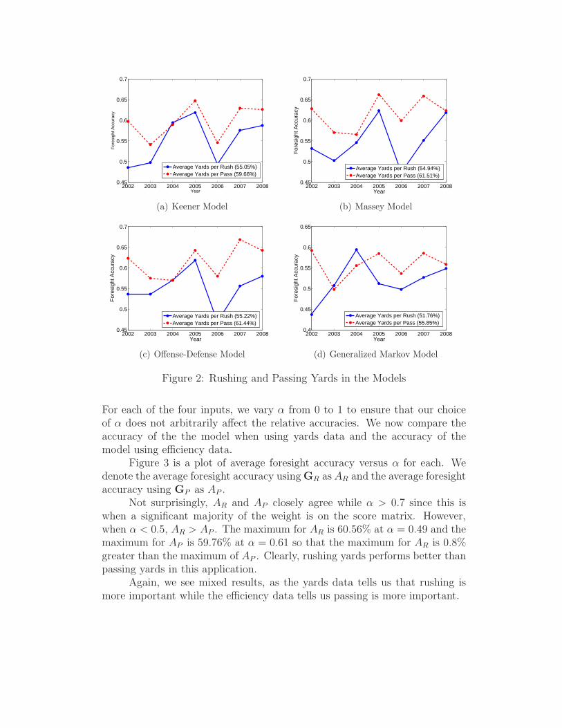
Now, Figure 2 shows the same plots, using average yards per rush andaverage yards per pass as input.

We can see that the average foresight accuracy of when using averageyards per pass is 4.61% higher in the Keener model, 6.57% higher in the

2002 2003 2004 2005 2006 2007 20080.45

0.5

0.55

0.6

0.65

0.7

Year

For

esig

ht A

ccur

acy

Rushing Yards 58.96%Passing Yards 55.44%

(a) Keener Model

2002 2003 2004 2005 2006 2007 20080.45

0.5

0.55

0.6

0.65

0.7

Year

For

esig

ht A

ccur

acy


(b) Massey Model

2002 2003 2004 2005 2006 2007 20080.45

0.5

0.55

0.6

0.65

Year

For

esig

ht A

ccur

acy


(c) Offense-Defense Model

2002 2003 2004 2005 2006 2007 20080.48

0.5

0.52

0.54

0.56

0.58

0.6

Year

For

esig

ht A

ccur

acy


(d) Generalized Markov Model

Figure 1: Rushing and Passing Yards in the Models

Massey model, 6.22% higher in the Offense-Defense model, and 4.09% higherin the Generalized Markov model, than the average foresight accuacy whenusing average yards per rush. Clearly, our results using yards and our resultsusing efficiencies conflict one another. The yards data implies that impliesthat rushing offense is more important while the efficiency data implies thatpassing offense is more important.

Since the Generalized Markov model is designed to use more than onestatistic, we next run it on a convex combination of scores and, individually,rushing yards, passing yards, average yards per rush and average yards perpass, as follows

GR = αS + (1 − α)R (15)

GP = αS + (1 − α)P (16)

Gr = αS + (1 − α)r and (17)

Gp = αS + (1 − α)p. (18)

2002 2003 2004 2005 2006 2007 20080.45

0.5

0.55

0.6

0.65

0.7

Year

For

esig

ht A

ccur

acy

Average Yards per Rush (55.05%)Average Yards per Pass (59.66%)

(a) Keener Model

2002 2003 2004 2005 2006 2007 20080.45

0.5

0.55

0.6

0.65

0.7

Year

For

esig

ht A

ccur

acy


(b) Massey Model

2002 2003 2004 2005 2006 2007 20080.45

0.5

0.55

0.6

0.65

0.7

Year

For

esig

ht A

ccur

acy


(c) Offense-Defense Model

2002 2003 2004 2005 2006 2007 20080.4

0.45

0.5

0.55

0.6

0.65

Year

For

esig

ht A

ccur

acy


(d) Generalized Markov Model

Figure 2: Rushing and Passing Yards in the Models

For each of the four inputs, we vary α from 0 to 1 to ensure that our choiceof α does not arbitrarily affect the relative accuracies. We now compare theaccuracy of the the model when using yards data and the accuracy of themodel using efficiency data.

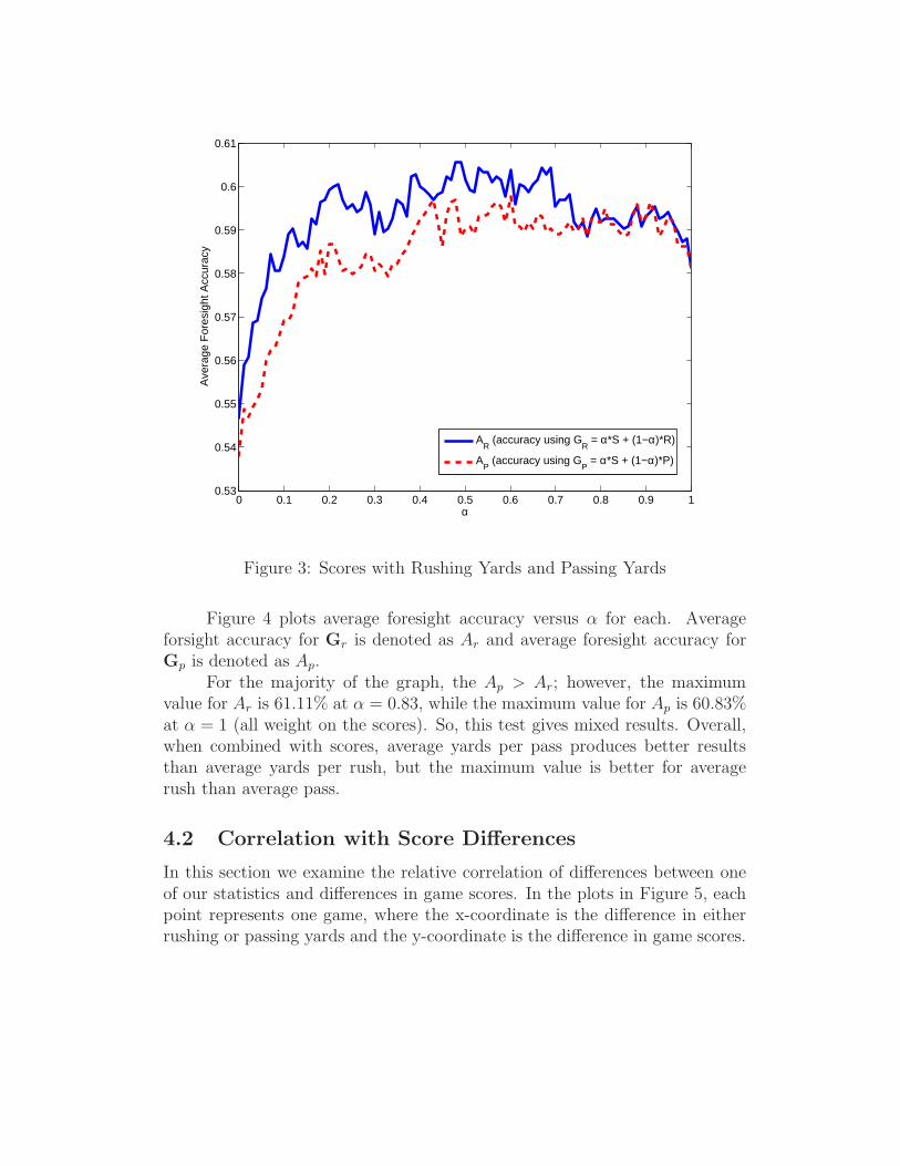
Figure 3 is a plot of average foresight accuracy versus α for each. Wedenote the average foresight accuracy using GR as AR and the average foresightaccuracy using GP as AP .

Not surprisingly, AR and AP closely agree while α > 0.7 since this iswhen a significant majority of the weight is on the score matrix. However,when α < 0.5, AR > AP . The maximum for AR is 60.56% at α = 0.49 and themaximum for AP is 59.76% at α = 0.61 so that the maximum for AR is 0.8%greater than the maximum of AP . Clearly, rushing yards performs better thanpassing yards in this application.

Again, we see mixed results, as the yards data tells us that rushing ismore important while the efficiency data tells us passing is more important.

0 0.1 0.2 0.3 0.4 0.5 0.6 0.7 0.8 0.9 10.53

0.54

0.55

0.56

0.57

0.58

0.59

0.6

0.61

α

Ave

rage

For

esig

ht A

ccur

acy

AR (accuracy using G

R = α*S + (1−α)*R)

AP (accuracy using G

P = α*S + (1−α)*P)

Figure 3: Scores with Rushing Yards and Passing Yards

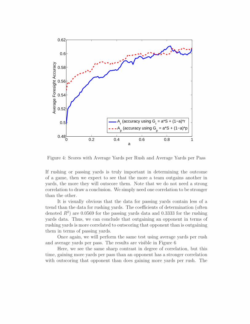
Figure 4 plots average foresight accuracy versus α for each. Averageforsight accuracy for Gr is denoted as Ar and average foresight accuracy forGp is denoted as Ap.

For the majority of the graph, the Ap > Ar; however, the maximumvalue for Ar is 61.11% at α = 0.83, while the maximum value for Ap is 60.83%at α = 1 (all weight on the scores). So, this test gives mixed results. Overall,when combined with scores, average yards per pass produces better resultsthan average yards per rush, but the maximum value is better for averagerush than average pass.

4.2 Correlation with Score Differences

In this section we examine the relative correlation of differences between oneof our statistics and differences in game scores. In the plots in Figure 5, eachpoint represents one game, where the x-coordinate is the difference in eitherrushing or passing yards and the y-coordinate is the difference in game scores.

0 0.2 0.4 0.6 0.8 10.48

0.5

0.52

0.54

0.56

0.58

0.6

0.62

a

Ave

rage

For

esig

ht A

ccur

acy

Ar (accuracy using G

r = a*S + (1−a)*r

Ap (accuracy using G

p = a*S + (1−a)*p

Figure 4: Scores with Average Yards per Rush and Average Yards per Pass

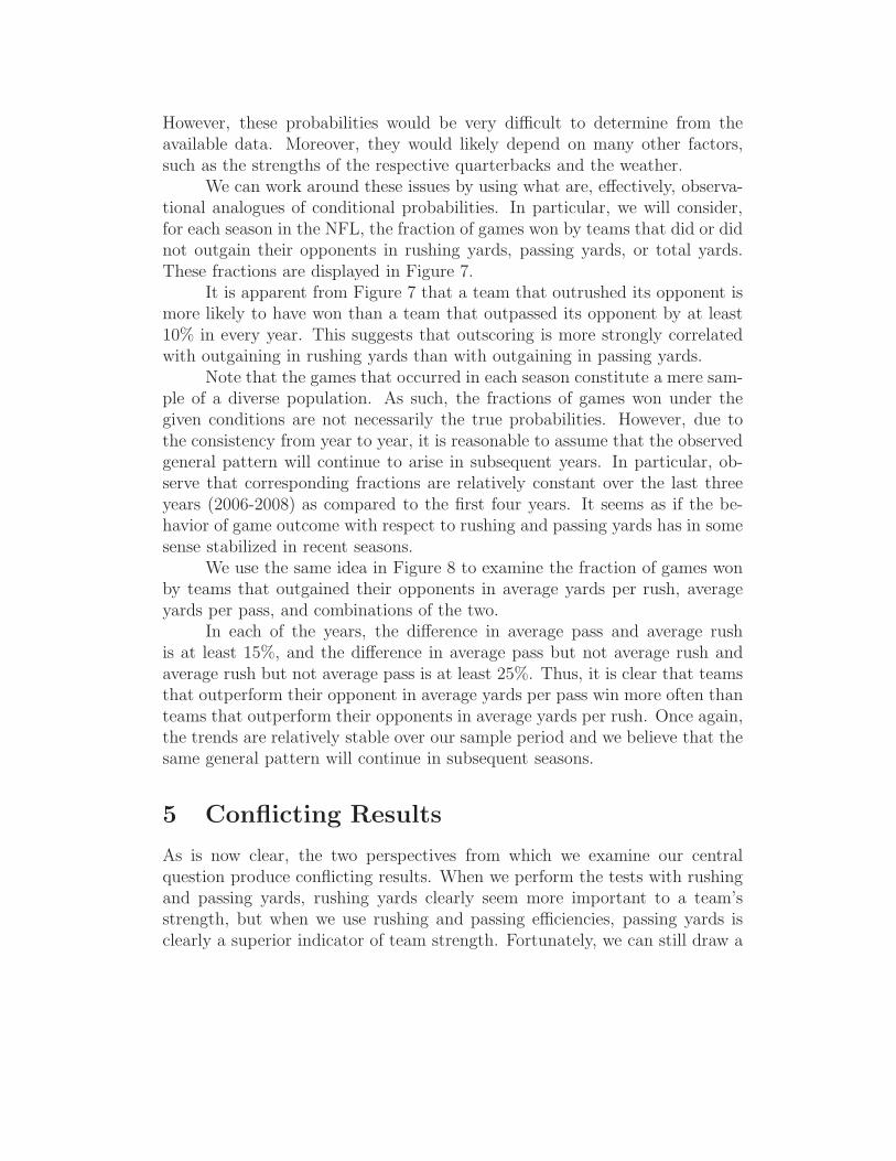
If rushing or passing yards is truly important in determining the outcomeof a game, then we expect to see that the more a team outgains another inyards, the more they will outscore them. Note that we do not need a strongcorrelation to draw a conclusion. We simply need one correlation to be strongerthan the other.

It is visually obvious that the data for passing yards contain less of atrend than the data for rushing yards. The coefficients of determination (oftendenoted R2) are 0.0569 for the passing yards data and 0.3333 for the rushingyards data. Thus, we can conclude that outgaining an opponent in terms ofrushing yards is more correlated to outscoring that opponent than is outgainingthem in terms of passing yards.

Once again, we will perform the same test using average yards per rushand average yards per pass. The results are visible in Figure 6

Here, we see the same sharp contrast in degree of correlation, but thistime, gaining more yards per pass than an opponent has a stronger correlationwith outscoring that opponent than does gaining more yards per rush. The

−400 −200 0 200 400−50

0

50

Passing Yards Difference

Sco

re D

iffer

ence

(a) Score Difference v. Passing Difference

−400 −200 0 200 400−50

0

50

Rushing Yards Difference

Sco

re D

iffer

ence

(b) Score Difference v. Rushing Difference

Figure 5: Least-Squares Plots with all Data Points

−10 −5 0 5 10 15−50

0

50

Difference in Average Yards per Pass

Sco

re D

iffer

ence

(a) Score Difference v. Passing Difference

−10 −5 0 5 10−50

0

50

Difference in Average Yards per Rush

Sco

re D

iffer

ence

(b) Score Difference v. Rushing Difference

Figure 6: Least-Squares Plots with all Data Points

value of R2 is 0.4701 for average yards per pass and 0.0324 for average yardsper rush.

4.3 Conditional Analysis

In order to analyze the relationship between rushing and passing yards fromanother viewpoint, we might consider certain conditional probabilities. Forexample, we might compare the conditional probability that a team outscoresits opponent given that it gains more rushing yards than its opponent withthe conditional probability that a team outscores its opponent given that itgains more passing yards than its opponent. Such a comparison would shednew light on the correlation between outscoring and outgaining in rushingyards as compared to that between outscoring and outgaining in passing yards.

However, these probabilities would be very difficult to determine from theavailable data. Moreover, they would likely depend on many other factors,such as the strengths of the respective quarterbacks and the weather.

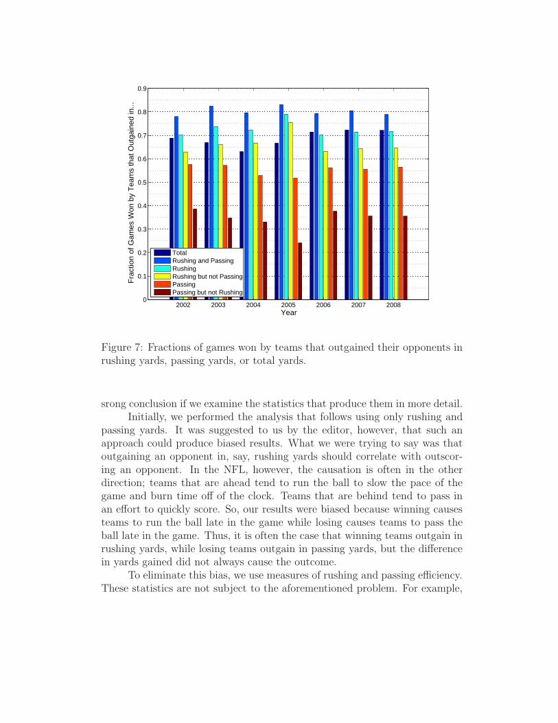
We can work around these issues by using what are, effectively, observa-tional analogues of conditional probabilities. In particular, we will consider,for each season in the NFL, the fraction of games won by teams that did or didnot outgain their opponents in rushing yards, passing yards, or total yards.These fractions are displayed in Figure 7.

It is apparent from Figure 7 that a team that outrushed its opponent ismore likely to have won than a team that outpassed its opponent by at least10% in every year. This suggests that outscoring is more strongly correlatedwith outgaining in rushing yards than with outgaining in passing yards.

Note that the games that occurred in each season constitute a mere sam-ple of a diverse population. As such, the fractions of games won under thegiven conditions are not necessarily the true probabilities. However, due tothe consistency from year to year, it is reasonable to assume that the observedgeneral pattern will continue to arise in subsequent years. In particular, ob-serve that corresponding fractions are relatively constant over the last threeyears (2006-2008) as compared to the first four years. It seems as if the be-havior of game outcome with respect to rushing and passing yards has in somesense stabilized in recent seasons.

We use the same idea in Figure 8 to examine the fraction of games wonby teams that outgained their opponents in average yards per rush, averageyards per pass, and combinations of the two.

In each of the years, the difference in average pass and average rushis at least 15%, and the difference in average pass but not average rush andaverage rush but not average pass is at least 25%. Thus, it is clear that teamsthat outperform their opponent in average yards per pass win more often thanteams that outperform their opponents in average yards per rush. Once again,the trends are relatively stable over our sample period and we believe that thesame general pattern will continue in subsequent seasons.

5 Conflicting Results

As is now clear, the two perspectives from which we examine our centralquestion produce conflicting results. When we perform the tests with rushingand passing yards, rushing yards clearly seem more important to a team’sstrength, but when we use rushing and passing efficiencies, passing yards isclearly a superior indicator of team strength. Fortunately, we can still draw a

2002 2003 2004 2005 2006 2007 20080

0.1

0.2

0.3

0.4

0.5

0.6

0.7

0.8

0.9

Year

Fra

ctio

n of

Gam

es W

on b

y T

eam

s th

at O

utga

ined

in...

TotalRushing and PassingRushingRushing but not PassingPassingPassing but not Rushing

Figure 7: Fractions of games won by teams that outgained their opponents inrushing yards, passing yards, or total yards.

srong conclusion if we examine the statistics that produce them in more detail.Initially, we performed the analysis that follows using only rushing and

passing yards. It was suggested to us by the editor, however, that such anapproach could produce biased results. What we were trying to say was thatoutgaining an opponent in, say, rushing yards should correlate with outscor-ing an opponent. In the NFL, however, the causation is often in the otherdirection; teams that are ahead tend to run the ball to slow the pace of thegame and burn time off of the clock. Teams that are behind tend to pass inan effort to quickly score. So, our results were biased because winning causesteams to run the ball late in the game while losing causes teams to pass theball late in the game. Thus, it is often the case that winning teams outgain inrushing yards, while losing teams outgain in passing yards, but the differencein yards gained did not always cause the outcome.

To eliminate this bias, we use measures of rushing and passing efficiency.These statistics are not subject to the aforementioned problem. For example,

2002 2003 2004 2005 2006 2007 20080

0.1

0.2

0.3

0.4

0.5

0.6

0.7

0.8

0.9

Year

Fra

ctio

n of

Gam

es W

on b

y T

eam

s th

at O

utpe

rfor

med

in...

Avg Pass and Avg RushAvg PassAvg Pass but not Avg RushAvg RushAvg Rush but not Avg PassNeither

Figure 8: Fractions of games won by teams that outperformed their opponentsin average yards per rush or average yards per pass.

a team behind for the whole game may pass the ball often and gain a dispro-portionate number of passing yards. However, the mere act of doing somethinga lot would not necessarily enhance their efficiency statistic, average yards perpass, since we divide by the total number of passing plays. Thus, we gain amuch better sense of how good the passing offense is, rather than just howmany yards they gained. We hold that this is a better measure of the strengthof a team’s offense than yards gained.

In light of these arguments, we will use the results obtianed when usingthe efficiencies to draw our conclusions. We have included all the informationin an attempt to more fully address the question and because the differentresults and the reasons for them are interesting in and of themselves.

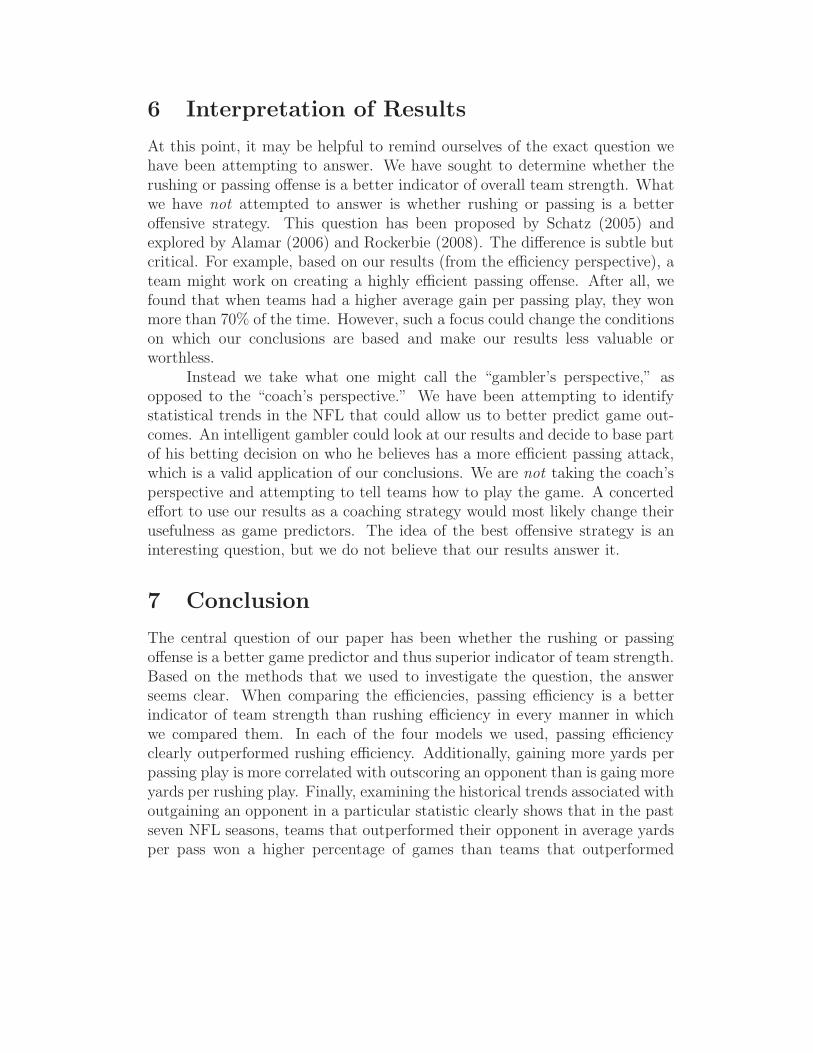
6 Interpretation of Results

At this point, it may be helpful to remind ourselves of the exact question wehave been attempting to answer. We have sought to determine whether therushing or passing offense is a better indicator of overall team strength. Whatwe have not attempted to answer is whether rushing or passing is a betteroffensive strategy. This question has been proposed by Schatz (2005) andexplored by Alamar (2006) and Rockerbie (2008). The difference is subtle butcritical. For example, based on our results (from the efficiency perspective), ateam might work on creating a highly efficient passing offense. After all, wefound that when teams had a higher average gain per passing play, they wonmore than 70% of the time. However, such a focus could change the conditionson which our conclusions are based and make our results less valuable orworthless.

Instead we take what one might call the “gambler’s perspective,” asopposed to the “coach’s perspective.” We have been attempting to identifystatistical trends in the NFL that could allow us to better predict game out-comes. An intelligent gambler could look at our results and decide to base partof his betting decision on who he believes has a more efficient passing attack,which is a valid application of our conclusions. We are not taking the coach’sperspective and attempting to tell teams how to play the game. A concertedeffort to use our results as a coaching strategy would most likely change theirusefulness as game predictors. The idea of the best offensive strategy is aninteresting question, but we do not believe that our results answer it.

7 Conclusion

The central question of our paper has been whether the rushing or passingoffense is a better game predictor and thus superior indicator of team strength.Based on the methods that we used to investigate the question, the answerseems clear. When comparing the efficiencies, passing efficiency is a betterindicator of team strength than rushing efficiency in every manner in whichwe compared them. In each of the four models we used, passing efficiencyclearly outperformed rushing efficiency. Additionally, gaining more yards perpassing play is more correlated with outscoring an opponent than is gaing moreyards per rushing play. Finally, examining the historical trends associated withoutgaining an opponent in a particular statistic clearly shows that in the pastseven NFL seasons, teams that outperformed their opponent in average yardsper pass won a higher percentage of games than teams that outperformed

their opponent in average yards per rush. The only evidence against our claimis the mixed results from the second application of the Generalized Markovmodel. Recall that though the accuracy using scores and passing efficiency wasgenerally higher, the maximum average foresight accuracy was higer usingscores and rushing efficiency than when using scores and passing efficiency.Thus, if one wishes to predict the outcome of a particular NFL game and cangauge the relative strengths of the two team’s rushing and passing games, oneis more likely to choose the winner if one picks the team with the strongerpassing game. For anyone serious about the business of game prediction, morevariables must be taken into account, but the relative strengths of the teams’passing games are certainly important to consider.

References

Benjamin C. Alamar. The Passing Premium Puzzle. Journal of Quantitative

Analysis in Sports, 2(4), 2006.

ESPN. NFL Expert Picks - Playoffs - Super Bowl, 2009. URLhttp://sports.espn.go.com/nfl/features/talent.

Anjela Y. Govan. Ranking Theory with Application to Popular Sports. PhDthesis, North Carolina State University, 2008.

Anjela Y. Govan, Amy N. Langville, and Carl D. Meyer. Offense-DefenseApproach to Ranking Team Sports. Journal of Quantitative Analysis in

Sports, 5(1), 2009.

James P. Keener. The Perron-Frobenius Theorem and the Ranking of FootballTeams. SIAM Review, 1993.

Kenneth Massey. Statistical Models Applied to the Rating of Sports Teams.1997.

Carl D. Meyer. Matrix Analysis and Applied Linear Algebra. Society forIndustrial and Applied Mathematics, Philadelphia, PA, 2000.

Duane W. Rockerbie. The Passing Premium Puzzle Revisited. Journal of

Quantitative Analysis in Sports, 4(2), 2008.

Aaron Schatz. Football’s Hilbert Problems. Journal of Quantitative Analysis

in Sports, 1(1), 2005.

Richard Sinkhorn and Paul Knopp. Concerning Nonnegative Matrices andDoubly Stochastic Matrices. Pacific Journal of Mathematics, 21(2):343–348, 1967.

journal of quantitative analysis in...

Documents