Journal of the Statistical and Social Inquiry Society of Ireland, Vol. XXIV, Part II, 1979/80, pp. 1-28.

ECONOMIES OF SCALE AND TECHNICAL CHANGEIN ELECTRICITY PRODUCTION IN IRELAND

M.J. HARRISON*

(Read before the Society, 8 November, 1979)

1. INTRODUCTION

Knowledge of the structure of production in public-utility enterprises is of considerableeconomic importance. Such things as the nature and extent of returns to scale andreturns to individual factor imputs, the degree of substitutability between inputs, and theextent of allocative inefficiency and X-inefficiency may have bearings on various issues atthe plant, firm and industry levels. For example, the nature and extent of returns to scaleare known to have important implications for, amongst other things, investment policiesin growing industries and the institutional arrangements necessary to achieve an optimalallocation of resources (Nerlove 1963, p. 167). But of course, whatever the particularconcern, the formulation of precise policy prescriptions or appraisals requires suitablequantificationof the production structure at the appropriate level.

The main purpose of this paper is to analyse the structure of production in the Irishelectricity supply industry at the level of the individual thermal generating station. Suchan analysis has not previously been carried out for Ireland, despite the abundance andavailability of good-quality data; but various econometric studies of the electric-powerindustry have been reported for several other countries, and most of these have made useof some explicit production function. This production function approach is adopted here.

More specifically, the study is based on the use of the so-called non-homothetic Leontiefproduction function which was developed recently by Lau and Tamura (1972). The primeobjective is to estimate the parameters of this function using pooled cross-section andtime-series data, and to assess its adequacy as a description of the thermal electricitygeneration process at the plant level. A second objective is to use the estimated parametersto investigate certain matters which may be of relevance and interest to policy-makers,such as how the scale of the plant affects the quantities used of each of four major inputs,namely, capital, fuel, energy and labour; how variations in the intensity of the use of theplant affect the quantities of inputs used; and whether and how the pattern of technicalchange in plants has affected the use of individual inputs. The analysis includes explicittesting of hypotheses concerning the homotheticity of the production structure, theconstancy of returns to scale, and the existence and Hicksian neutrality of embodied anddisembodied technical progress. It is hoped that such an econometric analysis will pro-vide a useful supplement to the considerable amount of engineering and other informationon electricity generation at plant level.

In addition to the econometric analysis, the paper contains a small amount of back-ground material. Section 2 contains a brief sketch of the Irish generation system and theelectricity production process; the latter may be viewed as providing the essential rationalefor the choice of production function. Section 3 contains a brief outline of the relevantearlier econometric research on electricity production, and a general account of the non-homothetic Leontief production function and its properties. Section 4 reports the

*The author is grateful to Mr. J.B. O'Donoghue, Director of Finance, ESB and Mr. H. Maume, Deputy-Head of Generation, ESB for helpful discussions and the unpublished data they provided; to JonathanHaughton and Sean Nolan for research assistance during the early stages of the project; and toProfessor D.F. McAleese and Mr. J.W. O'Hagan, Trinity College, Dublin, and a referee for helpfulcomments on an earlier draft of this paper.

I

econometric analysis proper. It includes a detailed account of the specification andmethodology for estimation of the particular model used, comments on the data availablefor individual generating stations and the derived data used for the analysis, and a discussionof the results.1 As will be seen, the main findings to emerge are that the chosen productionfunction describes the data well; that there are substantial economies in the use of labourand energy in electricity production, and smaller economies in the use of capital and fuel;and that the impact of embodied and disembodied technical change on the use of factorshas been slight. A summary and conclusion are given in Section 5. The conclusion includescomments on the value for policy purposes of the main findings of the analysis.

2. PRODUCTION OF ELECTRICITY IN IRELAND

The ESB Generation System2

The generation of electricity in Ireland — and its transmission, distribution and sale —is undertaken by the Electricity Supply Board (ESB), a corporation established understatute in 1927 and now the largest of the state-sponsored bodies and, in terms of capitalassets, probably the largest industrial concern in the country. However, due mainly toGovernment policy to utilise indigenous resources as far as possible, the generation systemof the ESB is essentially a small unit system. It currently comprises 28 generating stations- 18 thermal and 10 hydro - and has a total installed capacity of about 2,000 megawatts(MW), roughly four times more than what total capacity was in I960.3 Since the mid-1960s, when the scope for further feasible development of peat and conventional hydrogeneration diminished, the system has made increasing proportional use of thermal plants,especially oil-fired plants, and thermal installations now account for about 80 per cent ofthe total capacity and about 92 per cent of actual electricity production. Of the remain-ing capacity accounted for by hydro stations, over half is provided by the new 292 MWpumped storage station at Turlough Hill. Immediately prior to the commissioning of theTurlough Hill station the share of thermal capacity was about 87.5 per cent of the total.By comparison, the corresponding shares in 1950 and 1960 were about 53 per cent and69 per cent, respectively.

The present study is concerned solely with the production of electricity from thermalenergy sources, of which there are three in wide use by the ESB, namely, peat, coal andoil. While gas is expected to become increasingly important in the near future, only verysmall amounts have been used to date in the Poolbeg station in Dublin. Of the 18 thermalstations in the system, six are designed to burn sod peat, four to burn milled peat, one toburn sod peat and milled peat, one to burn Irish semi-bituminous coal, and the remainingsix to burn oil.4

In addition to differences in the type of fuel used, there are wide variations amongstthese plants with respect to age of equipment, capacity, and the number and sizes ofgenerating sets. Plant capacity, for example, varies from 5 MW, as in the case of each ofthe four sod peat stations in the West of Ireland, to 620 MW, the capacity of the Tarbertoil-fired station in County Kerry with an average capacity of approximately 112 MW perstation; the capacity of individual generating sets varies from 5 MW to 270 MW, thesize of the recently commissioned set in the Poolbeg oil-fired station in Dublin, although31 out of a total of 48 sets have a capacity of less than 20 MW. Only six sets have acapacity greater than 100 MW: one in the Great Island station in County Wexford, two inthe Tarbert station, and three in the Poolbeg Station.

There are, therefore, likely to be differences in the efficiencies of individual stations,even for a given type of fuel. Naturally, it is the older (pre-1964) stations, with theirsmaller sets, lower steam pressures, and higher labour requirements, that are the leastefficient. The more modern peat, and particularly oil, installations probably have signifi-cantly higher efficiencies, largely by virtue of their greater size and technically moreadvanced equipment.

The use of generating stations to meet a given demand for electricity, referred to asload-despatching, is influenced by the ESB's obligation to consume a certain amount of

native peat each year. However, subject to this constraint, and certain other physicalconstraints, such as those imposed by the breakdown of equipment or its shut-down formaintenance purposes, the ESB attempts to utilise its capacity so as to produce electricityas economically as possible. In practice this means that base load is covered by the modernoil-fired stations (and some conventional hydro stations) and the intermediate load rangeby the older oil and peat-fired stations, while peak load is covered by the North Wall oil-fired plant in Dublin (and by the hydro stations with storage facilities). One obviousresult of this load-despatching policy is that different plants are subject to differentdegrees of capacity utilisation. This is taken into consideration in the formulation of themodel in Section 4.

The Electricity Production Process5

The fundamental function of the generating system, of course, is to convert energyfrom the various sources into electricity. In the thermal stations, the same basic processis used to carry out this function. Briefly, the fuel is burned to produce hot gases whichare used, firstly, in an economiser to pre-heat feed-water entering the boilers, and secondly,in the boilers themselves to convert the water to steam. The temperature of the steamleaving the boilers is increased in a superheater and the steam is then used to operateturbines which turn the generators to produce the electricity. The exhaust steam, afterleaving the turbines, passes through a condenser and is converted back to water to bepumped, via the feed-water heater and economiser, back to the boilers.

For the purposes of this study it is convenient to distinguish four inputs to this pro-duction process, each being, in principle, a flow variable. Firstly, a capital input (C) whichaccounts for the service flow provided by the physical stock of equipment: the boilers,turbines, generators, pumps, etc. Secondly, a fuel or raw material input (F) which, as hasalready been mentioned, may be a flow of peat, coal or oil. Thirdly, an energy input (E)which accounts for the flow of power required to operate some equipment, such as fuel-handling machinery and pumps, and to provide lighting; power stations actually use aportion of their own output for these purposes. Fourthly, a labour input (L) whichaccounts for the flow of services provided by the staff that operate and maintain the plant.There is of course a single homogeneous flow of output (Q) from the production process.

The process is highly capital intensive and is subject to rigid technological requirementswhich preclude the ex post possibility of substitution of inputs for a given level of output.It is also thought to be characterised by substantial economies of scale and the availableevidence lends firm support for this view. It has, of course, as has already been mentioned,been influenced by the rapid technical progress experienced during recent years. Theactual degree of capacity utilisation varies amongst plants and is determined essentiallyby load-despatching policy.

3. ELECTRICITY PRODUCTION AND THE PRODUCTION FUNCTION

Previous StudiesThe production of thermal electricity at the plant level has been analysed in terms of

the production function concept by several authors. The work of Komiya (1962), Barzel(1964), Dhrymes and Kurz (1964), and Galatin (1968) is of particular relevance to thepresent study and will be referred to periodically throughout the paper. Their respectivesets of results, though based on data for the United States, constitute a valuable basis ofcomparison for the results presented in Section 4 and they will be referred to again inthat Section. Immediately following is a brief account of the basic approaches employedby these authors.

Komiya, using cross-section data, estimated production functions for several groups ofplants categorised by their technological vintage and fuel-type. He found that a substitutionmodel based on the Cobb-Douglas function was an unsatisfactory means of analysis. Amore successful model, which he called a 'limitational model', was based on a system ofinput demand equations relating capital, fuel and labour, respectively, to a measure of

plant capacity, as follows:

_fl. ix.X.=a .Q *N \ i = C, FandL, (1)

where X. denotes the quantity of the ith input per generating-unit (set) required at thecapacity level of operation, Q the average size of the generating-unit in megawatts, and Nthe number of generating-units in the same plant. The a., |3. and /x. are constants; theeconomic interpretation of such parameters is discussed, in relation to the actual modelemployed in the present study, in Section 4. The impact of technical change was assessedby Komiya on the basis of the differences in the estimated input functions for his variousvintage groups.

The studies of Barzel, Dhrymes and Kurz, and Galatin were also based on sets ofinput functions similar to (1), but they each incorporated modifications of specificationand employed various procedural innovations. In particular, Barzel introduced the degreeof capacity utilisation, measured by the observed load factor,6 into his specification, and,using cross-section and time-series data, attempted to quantify the effect of technicalchange by the use of dummy variables for the various vintages of plant. Dhrymes andKurz, unlike all the other authors, derived their equations explicitly, on the assumptionof exogenous demand and prices, and cost-minimising behaviour subject to the constraintimposed by the underlying production function, which they postulated to be of the CES-type. Thus their equations contained relative prices, as well as output, as explanatoryvariables. However, in the light of their initial estimates, which were based on cross-sectiondata on plants grouped by vintage and size, they replaced their original labour inputfunction by an equation akin to (1); by relating the labour requirement to output only,this better reflected the situation in electricity production, namely, that labour is not asubstitute for capital or fuel.7 Galatin, critical of various aspects of the previous studies,especially their neglect of the problem of 'machine-mix', formulated a model which tookexplicit account of machine-mix and degree of capacity utilisation. Indeed, for his fuelequation, he took the machine - i.e., the turbine-generator set and its associated systemof boilers and ancillary equipment — as his unit of observation, rather than the plant.However, like his capital and labour equations, the fuel equation had to be estimatedfrom data on plants, and this posed certain aggregation problems (see Galatin 1968, Sec.5.2). Largely because of these problems, Galatin used a linear functional form for hisequations rather than a form which was linear in the logarithms of the variables as previouswriters had done. His estimation was undertaken using cross-section and time-series dataon plants categorised according to vintage, size and fuel-type.

It is noteworthy that a similar functional form to (1) has been used in several studiesof production in other industries characterised by limited factor substitutability. Of thesestudies, the one by Lau and Tamura (1972) for the Japanese petrochemical industry isespecially significant in that it includes the first proof that a system of input functionssuch as (1) may be derived from cost minimisation subject to a production function con-straint. Previously, such formulations had been distinguished from those, such as theequations of Dhrymes and Kurz, that were derived on the explicit assumption of optimisingbehaviour (see, for example, Galatin 1968, Ch. 4). Moreover, Lau and Tamura present anexplicit derivation of the class of production functions underlying the derived inputfunctions, namely, the non-homothetic Leontief production function (hereafter NHLproduction function). A brief explanation of this function and its properties is given inthe following subsection.

The NHL Production FunctionThe NHL production function for an output-taking, cost-minimising undertaking,

which gives rise to input equations such as those in (1), may be written as

Q = 3>(X) = min [f H*)] , i = 1,2,3,. .. ,k, (2)i

where Q denotes the quantity of output, and X. the quantity of the ith input, f H-) *s a

generalised inverse of the function f.(.) which has the properties that fj(Q) is a positivereal-valued function, defined and finite for all finite Q > 0 with fj(O) = 0, and is a non-decreasing lower semicontinuous function in Q which becomes unbounded as Q becomesunbounded.8 Of course, the ff(Q) are just the right hand sides of the derived input demandfunctions for the k factors employed in the production process; these may be written asXj = f|(Q), i = 1,2,3,. . . ,k. Embodied and disembodied technical change may be incor-porated into the NHL production function simply by writing the f^Q) as functions ofplant vintage (v) and time (t) as well as of the quantity of output. The system of inputfunctions then becomes XL = f^Q/^t), i = 1,2,3,. . . k. Lau and Tamura (1972, p. 1174)show that on the assumption of Hicksian neutrality for both forms of technical changethis may be written as

X. = f.(Q,v,t) = fi*(Q)V(v)T(t). (3)

Underlying these formal definitions is a basically simple idea. Equation (2), in essence,merely states that the NHL production function is the kind of function which, in termsof the concepts of elementary economics, has L-shaped isoquants — hence the nameLeontief. Thus it has the property of zero elasticities of substitution between all pairs ofinputs, and the derived input demand functions are independent of prices. In fact, theNHL function is the most general production function with zero elasticities of substitution,and is a member of the CES class of functions. As its name implies, another property ofthe function is that it is not necessarily homothetic; that is, its expansion path is notnecessarily a straight line through the origin. Hence the optimal proportions of factorsmay vary across plants if plant output levels differ. Another property of the NHL produc-tion function is that the degree of returns to scale may be different for each factor input.Some further explanation of this last feature may be useful.

The 'technical' meaning of returns to scale relates to the impact on output of equi-' proportionate changes in the quantities of all inputs. In the context of the NHL productionfunction, however, an alternative interpretation of returns to scale is adopted. This,perforce, focuses on the effect on output of scale changes in the form of proportionalvariations in the quantities of all inputs corresponding to movements along a plant'sexpansion path. These proportional variations will not be equal, and the technical definitionof returns to scale will therefore not apply, unless the expansion path is a straight linethrough the origin, which, as has been stated, is not necessarily the case for a NHL pro-duction function. Incidentally, this alternative interpretation of the concept correspondswith the approach, sometimes used in economics, of relating returns to scale to thebehaviour of average costs.

4. ECONOMETRIC ANAL YSIS OF ESB PRODUCTION

Model SpecificationThe characteristics of the electricity production process in thermal plants, which were

described in Section 2, themselves suggest that a fixed factor proportions model is aplausible model for econometric analysis. The empirical findings of Komiya, Barzel,Dhrymes and Kurz, and Galatin, in particular, provide considerable support for this view;the theoretical work of Lau and Tamura reinforces it further. For the purposes of thisstudy, therefore, a NHL production structure was hypothesised for thermal electricitygeneration at the plant level in the Irish generation system. It does not follow of course,as Nerlove (1963, p. 173) has pointed out, that the NHL structure would necessarily bethe most appropriate to assume for a higher level of aggregation, such as the firm level.

The input demand functions which derive from the NHL production function, andwhich provide the means of estimating it, may take various forms. For this study, follow-ing Komiya, Barzel, and Dhrymes and Kurz, functions which are linear in the naturallogarithms of the variables were chosen. Apart from the computational convenience of

using log-linear or constant elasticity equations, there are sound theoretical reasons forpreferring this functional form as Haldi and Whitcomb (1967, pp. 375-376) have pointedout.

Unfortunately, there is not the same consensus as to the precise specification of thevariables that should enter the input functions. The formulation adopted here was basedon that used by Lau and Tamura, which allows explicitly for the presence of embodiedtechnical change. This form was chosen because, although pooled cross-section and time-series data were available, the number of thermal plants in Ireland is very much smallerthan the number in the United States, and consequently both the method of using severalvintage groups of plants, and the method of using vintage dummy variables, were con-sidered unfeasible with Irish data for degrees of freedom reasons. Unlike the Lau andTamura model, however, the model used in the present study also allows for the presenceof disembodied technical change. Thus, in accordance with equation (3), the basic systemof input equations postulated were as follows:

logeXipt = log.cn + /¥°geQpt + TiVp + 5.t + eipt

i = C , F , E , L , p = l , 2 , . . . , N , t = l , 2 , . . . , T , (4)

where X is plant input per time-period, Q is plant output, v is plant vintage, t is the time-period and e is an additive stochastic disturbance; i refers to the four inputs previouslydefined, p to the particular plant; the av j3., 7. and 8{ are unknown constants.

The unqualified use of output as an independent variable is not, however, entirelysatisfactory in the context of electricity generation, since plants of widely differing sizesmay produce a similar output, but without requiring the same amounts of inputs. It istherefore desirable to attempt to distinguish between the effects of size and the degree ofcapacity utilisation, especially, it seems, in the case of the labour, fuel and energy inputrelations. Size and utilisation factors can be introduced directly by means of the relation-ship between output and the capacity and load factor of a plant. For estimation purposes,therefore, the preferred system of input functions was of the form:

logeXipt = a*+ ftlog^ + XilogeL;t + 7ivp + Sjt + eipt> (5)

where Q* denotes plant capacity (size), and L* denotes the overall plant load factor;

Clearly, |3j > 1 implies the existence of diseconomies of size with respect to input i;j3j = 1 implies constant returns to size; j34 < 1 implies increasing returns to size. Similarly,X | > 1 , Xj=l, Xj <C 1 imply the existence, respectively, of diminishing, constant andincreasing returns to degree of capacity utilisation with respect to input i. Iffy f \ , thedecomposition of output into its capacity and load components is, of course, entirelyjustified. Also y>v 5{>0 implies, respectively, embodied and disembodied technicalretrogression; y-v 8{ = 0 implies zero technical change of both kinds; 7i? 6 j < 0 impliestechnical progress of both kinds. Furthermore, it can be verified (see Lau and Tamura1972, pp. 1174-1175) that given the type of specification in (5), a necessary and sufficientcondition for homotheticity is that for all i, j3j = \ = cx, where cx is a constant; a necessaryand sufficient condition for overall constant returns to size is j3j= 1, for all i, and anecessary and sufficient condition for overall constant returns to degree of capacityutilisation is \ = 1, for all i;9 a necessary and sufficient condition for Hicks neutraltechnical change of both kinds is that for all i, 7. = c2 and d{ = c3, where c2 and c3 areconstants; and a necessary and sufficient condition for zero technical change is y{ = d{ = 0for all i.

A specification of the properties of the stochastic disturbance term was chosen toyield a pooled cross-section and time-series model which allowed, for each input function,the possibility of heteroscedasticity and correlation amongst plants, and time-wise auto-correlation for individual plants, as follows:

E(e?,t) = aO), E(eipteip,t) = c$\ (p t P*X

a n d eiPt = ^ipeiP(M) + u i P f w h e r e u iPt ~ N(O,4>(p>),

and E(e ip(t.1)Uipt) = 0, E(u i p tu i pn) = * $ . (p t p*), (6)

E(uiptuips) = O(t?ts),

i = C,F,E,L, p,p* = 1,2,... ,N, t,s = 1,2,... ,T.

The initial value of e- v ei o , w a s assumed to have the properties €j o ^ N(O,$(pV1—p? ) and E(ej o€j * o ) = 4>(p)»/l-pj Pj * for p ̂ p*. The disturbance variance-covariance

matrix, £2j, for the ith input demand function of the model, may therefore be written, interms of the typical (pp*th) element, as

' w h e r e 2 . nT-11 Pip* Pip* Pip*

Pip ] P.ip* Pip"*2

(7)

A stoachastic specification similar to this is described in Kmenta (1971, pp. 512-513).Such a model is not only much more comprehensive, but, it would seem, much morerealistic for the purposes of analysing electricity production data than the kind of sto-chastic specifications used in previous studies. These previous specifications are alludedto in the following subsection.

Of the explanatory variables in the system of equations (5), which for the purposesof this study is viewed as relating to an ex post underlying NHL production function,vintage and time are of course exogenous. Plant size and load factor are also assumed tobe exogenous. Once a generating station is built, output from the plant, and hence itsload factor, are largely determined by the overall demand for electricity and the load-despatching policy of the generation authority. While for the firm as a whole the demandfor output from a given plant is clearly not exogenous, the view was taken, as in previousstudies, that at the level of the plant, output and load factor are determined by an exogenousdemand. Therefore the plant was assumed to behave essentially as an output-takingconcern which attempts to minimise its cost of production. This does not seem to be toofar out of line with stated ESB policy. It would, of course, be more difficult to sustainan argument that in the ex-ante choice of plant design, planned output (capacity) isexogenous.

It should perhaps be noted that the hypothesised input functions abstract from theproblem of the machine-mix of plants. As has already been mentioned, Galatin has beencritical of such formulations. However, due to the small number of Irish generatingstations, Galatin's approach to the problem, namely, of grouping plants by the numberand size of their turbine-generator sets, was not feasible for this study, and no alternativeapproach was found.

Model EstimationIn previous electricity production studies, ordinary least squares (OLS) has invariably

been used to estimate the coefficients of the input functions. Although little attentionseems to have been given to the stochastic specification of the functions, it may be pre-sumed that appropriate assumptions about the disturbance terms were made. Unfortunately,no test statistics relating to residual analysis were published by which to assess the validityof these assumptions, at least for the various production studies mentioned earlier. How-ever, Galatin did note that in the case of his fuel function, the classical assumptions are

violated by the presence of heteroscedasticity introduced by his aggregation methodology.It is perhaps more important to note that the studies which used OLS assumed, implicitly

at least, that no correlation existed between the disturbances of different input functions.If such correlation exists — and it seems reasonable to assume it does for a given plant, ifnot between plants — then OLS estimation of the separate input functions would be astatistically efficient technique to use only if all the input functions contained the sameexplanatory variables and there were no restrictions on their parameters. Otherwise themethod of estimating seemingly unrelated regressions due to Zellner (1962) would berequired for efficient estimation. In fact, neither Komiya, Barzel, nor Galatin used thesame set of explanatory variables for all their input functions, although they all usedOLS.10

In this study, this uniformity of input equations is assumed, so that estimation ofequations individually may be considered. Despite this, OLS would not yield efficientcoefficient estimates due to the nature of the stoachstic properties specified in (6). OLSwould, however, give estimates which were unbiased and consistent, and for practicalexpediency could be used. Theoretically, a preferable estimator would appear to be themodified Aitken estimator

Ai = (z'd-iiz)-Hz'^-i1xi), (8)

whose asymptotic variance-covariance matrix is

V(/ii) = (ZU i1Z)-1 , i = C,F,E,L, (9)

where Z is the NT X 5 matrix of pooled cross-section and time series observations on theexplanatory variables, including the dummy variable unity to account for the intercept,X. is the vector of NT observations on the i*h input, and SYj1 is the NT X NT estimateddisturbance variance-covariance matrix, and /ij = \a{ |3j \ 7j 5j J ' the vector of para-meter estimates, for the ith input function.

The following procedure based on OLS may be used to provide a matrix tt. whoseelements are consistent estimates of the elements of the unknown matrix £2.. Firstly, OLSis applied to all of the pooled data and the resulting residuals, e4 t , used to estimate p- by

the formula p ip = | e ip te ip(M)/ g e?p(t.1}, p = 1,2,. . . ,N, i = C,F,E,L. The p ip are con-

sistent estimates of the p i p . Secondly, the p- are used to transform the data to 'gener-

alised differences': xipt = Xipt-PipXip(t_1)5 q* = Q* -p ipQ*, etc. Thirdly, OLS is applied to

the transformed data and the residuals from this regression, "eipt, used to estimate the

variances and covariances of the eipt, that is, the o#) and a^*, by s£p)* = ^pWl-PipPip*'

where i>$* = j ^ e ipte ip* t/T-5-1, p,p* = 1,2,. . . ,N, i = C,F,E,L.

This approach to the estimation of (5) can be simplified by applying the modifiedAitken formulae to the transformed data, that is, by using the estimator

Ai= ( z ' ^ z y H z ^ x . ) , (10)

with the associated asymptotic variance-covariance matrix

^ 1 z y 1 , (11)

where z denotes the transformed explanatory data matrix and ^f the estimated variance-covariance matrix. The estimate ^ is of order N(T-l) X N(T-l) and, in terms of the

typical element, may be written * . = [<££$* I-r-i] »where IT.j is the identity matrix

of order T-1, and the <^* may be obtained as previously indicated. The orders of z andx. are similarly reduced by N due to the transformation of variables. In general the valueof Aj would not be expected to be identical to that of Ai? but the asymptotic properties ofthe two estimators are the same.

The approach is, of course, well-known, and has been discussed by Zellner (1962) andTelser (1964) who have shown that both variants of the estimator, (8) and (10), have thesame asymptotic properties as Aitken's estimator, that is, they are consistent, asymp-totically efficient and asymptotically normal.11 The gain in efficiency over OLS dependson the values of the off-diagonal elements in $2. (in the present case, the extent to whichthe o([K and p ip differ from zero), the correlation of the explanatory variables for dif-ferent Pcross-sectional units (plants), and on whether shift variables are included in theequation (see Zellner 1962, or Balestra and Nerlove, 1966, p. 597).

DataA considerable amount of reliable technical and production data on the Irish generating

stations is available from the annual reports of the ESB. Specifically, the reports give, foreach plant, information on its capacity in megawatts, its annual gross and net output, andhence its own consumption of electricity, in millions of kilowatt-hours (units), its annualpercentage plant load factor, its fuel type, its numbers of turbine-generating sets andboilers, as well as a small amount of works cost information. The reports do not containinformation on the fuel consumption, manning and capital cost of plants. However, theESB kindly made this additional information available to the author. The plant fuelconsumption figures provided were in thousands of tons per year, the labour figures werethe average number of employees in each plant per year, and the capital figures were thetotal capital cost of each plant sub-divided into the cost of buildings (wharfs, cooling-towers, etc.), equipment (turbines, boilers, etc.) and outdoor equipment (transmissionstation, fuel-handling, etc.).

For the purposes of analysis, the fuel input (XF) of a plant was measured in thousandsof tons of oil (or, in the case of peat and coal, oil-equivalents) per year; the energy input(XE) was taken to be the consumption of electricity by the plant measured, as published,in millions of units per year; the labour input (XL) was the number of man-years asprovided by the ESB. For the capital input (Xc) two alternative measures were used,namely, the overall cost of an installation deflated by the price index for capital goods,and the cost of indoor generating and ancillary equipment deflated by the price index fortransportable capital goods for use in industry, both indices having base 1953 = 100.12

For the explanatory variables, the following measures were used for each plant: for out-put (Q) the published figure for annual gross output in millions of units; for capacity(Q*) the published megawatt capacity figure, which is based on the name-plate ratings ofthe sets in a plant; for degree of capacity utilisation (L*) the published annual percentageplant load factor; for vintage (v) the year of installation of a plant, and for time (t) thedummy variable t = 1, 2, 3, . . . , T, with 1953 = 1.

It should be noted that of these various measures, those for labour, capital and capacitymay have serious shortcomings. For labour, 'average number of employees' is known tobe a potentially poor measure because, amongst other things, it takes no account ofdifferences in the length of the working day or week over time, nor of different types(operating, maintenance) and qualities of labour. It was used, as in previous studies, in theabsence of a readily available alternative.

Similarly, the problems associated with measuring the concept of the quantity ofcapital employed in a plant per time-period are well-known. The deflated value of thecost of capital would appear to be a suitable measure if the price index used as deflatoris the appropriate one; but an "appropriate" price index cannot be derived unless thequantity units for capital are already well-defined, which is the original problem. Measuresof capital used in other studies of electricity generation have included the number of setsand the installed capacity in a plant, but the former takes no account of differences insizes, and both ignore "quality" differences which may be important. Dhrymes and Kurz

(1964) used megawatt capacity times the sum of hours a plant was "hot", whether con-nected or not connected to load. Galatin (1968, p. 91) has criticised this measure andsuggested that the aggregate of capacity multiplied by the degree of utilisation in eachhour would be a better measure in the context of the Dhrymes and Kurz analysis. Thiskind of measure could not be used in the present study as the necessary information oncapacity utilisation per hour was not available to the author. Galatin himself, and Barzelbefore him, actually used the undeflated value of capital because of the unavailability ofwhat they considered to be a suitable deflator. In adopting the deflated capital cost asthe capital measure, the present study follows the approach of Komiya (1962).

The capacity measure, more surprisingly perhaps, may also be somewhat unsatisfactory,because name-plate ratings refer to the maximum output that can be achieved withoutover-heating. According to engineering studies, as Nerlove (1963, p. 181) has pointed out,generating units of the same size, general design and actual capability may show as muchas 20 per cent difference in rating. To the extent that this factor is significant, the plantload factor, used to measure the degree of capacity utilisation of plants, also becomesunreliable, of course. Since capacity and degree of capacity utilisation are explanatoryvariables, possible errors in their measurement are of particular concern in that they haveimportant implications for estimation. The likely impact of such errors on the results ofthe study is mentioned in the discussion in the following subsection.

The data on the remaining variables - X p , X£ , Q, v and t - are considered to be quitereliable and not prone to measurement error.

With the exception of the four small Western stations at Miltown Malbay, Screeb,Cahirsiveen and Gweedore, the observations on the variables were available for eachplant from its first full year of operation up to and including the year ending March,1976. In the case of the Western stations, only combined production and labour figureswere available. Therefore, having been commissioned within a year of each other, theywere regarded as a single operation for the purposes of analysis.

Analysis and ResultsIn accordance with the estimation methodology outlined earlier, the model as specified

by (5) and (6) was initially estimated by OLS regression using the pooled cross-sectionand time-series data on the thermal plants in the generating system. Because the charac-teristics of input demand functions may be expected to vary somewhat with the type offuel used — and the results of previous studies appear to confirm this - the data werestratified according to fuel-type and separate functions estimated for peat and oil plants.The single small coal-fired station at Arigna was excluded from the analysis. Moreover,even within the peat and oil categories, certain plants were excluded, and not all of theavailable observations on plants that remained in the sample were utilised. This wasessentially because use of the modified Aitken estimator - variant (8) or (10) — requiresthat the time-series on each plant contain the same number of observations. In fact, asmentioned in Section 2, there is considerable variation in the age of generating stations.

A further consideration was that in the interests of meaningful estimation, the vintage- i.e. year of installation - of each plant should adequately represent the state of thetechnology of production throughout the period covered by the data. In fact, manyplants have had additional generating sets installed since their original commissioning;and to the extent that the technical specification of these newer sets differs from thatof the original equipment, the notion of the vintage of a plant becomes difficult to define,and its representation by the year of initial installation difficult to interpret.

In view of these two considerations, the length (T) of the time-series for each fuelcategory was determined by the age in years of the newest plant, or the number of yearsin operation with equipment of the original vintage of the plant which operated for theshortest time with that equipment, whichever was the smaller, and provided a certainminimum number of observations was available. Thus, for the peat category, the valueof T was determined by the Lanesborough 'A' sod peat station, the period of operationbefore the installation of the Lanesborough 'B' milled peat equipment being 7 years. The

10

Lanesborough CB' plant was not included in the sample because from the date of itscommissioning, separate labour figures for it — and the Lanesborough 'A' plant — werenot available. The Ferbane milled peat station was not included because the 5 years ofoperation before additional equipment was installed was considered too short a period.For the oil category, T was determined by the Tarbert station on which there were 7annual observations available. The new oil-fired Poolbeg station was excluded becausethere were too few observations on it. In addition, the now obsolete, old Pigeon Housestand-by station was excluded from the analysis.

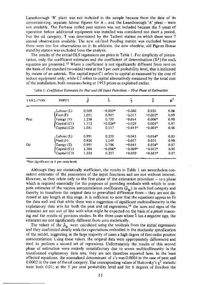
The results of the initial OLS regressions are given in Table 1. For simplicity of presen-tation, only the coefficient estimates and the coefficient of determination (R2) for eachequation are presented.13 Where a coefficient is not significantly different from zero onthe basis of the standard two-sided t-test at the 5 per cent probability level, this is indicatedby means of an asterisk. The capital input Cl refers to capital as measured by the cost ofindoor equipment only, while C2 refers to capital alternatively measured by the total costof the installation, both measures being at 1953 prices as explained earlier.

Table 1: Coefficient Estimates for Peat and Oil Input Functions - First Phase of Estimation

FUEL-TYPE

Peat

Oil

INPUT

Labour(L)Fuel (F)Energy (E)Capital (Cl)Capital (C2)

Labour(L)Fuel (F)Energy (E)Capital (Cl)Capital (C2)

0.5691.0511.2361.1121.051

0.9910.9260.9911.3041.331

X

-0.050*0.9070.755

-0.024*0.117

0.2531.1490.786

-0.006*0.257

7

-0.060-0.017-0.014-0.029-0.015*

-0.045-0.057-0.045-0.009*-0.030

6

0.050-0.002*

0.006*0.005*

-0.001*

-0.014*0.0310.034*

-0.012*-0.015*

R2

0.860.990.980.970.96

0.850.980.970.950.97

*Not significant at 5 per cent level.

Although they are statistically inefficient, the results in Table 1 are nevertheless con-sistent estimates of the parameters of the input functions and are not without interest.However, as they relate only to the first phase of the estimation procedure - to a phasewhich is required essentially for the purposes of providing residuals with which to com-pute estimates of the various autocorrelation coefficients (jSj ) in each fuel category andthereby to transform the original data to generalised difference form - they are not dis-cussed at any length at this stage. It is sufficient to note that the equations appear to fitthe data well and that while there was a suggestion of significant multicollinearity in theexplanatory data sets for both the peat and oil regressions,14 the sizes and signs of theestimates are not out of line with what might be expected on the basis of a priori reason-ing and the results of previous studies. In the three cases where X has a negative sign, theestimates are not significantly different from zero statistically.

The values of the p ip were calculated using the residuals from the initial regressionsand they conformed closely with the expectations embodied in the stochastic specificationof the model, suggesting in the large majority of cases a high degree of first-order positiveautocorrelation. Using these values, the original data were appropriately differenced andused to perform a second set of regressions. Unfortunately the results of this secondphase of estimation were entirely unsatisfactory due to severe multicollinearity in thetransformed explanatory data sets; they are not therefore reported here. In the leastaffected equations, the normalised determinant of z'z was 0.0004 in the case of peat and0.0002 in the case of the oil category. The corresponding values of Haitovsky's x2 statisticwere both 0.01; at the 5 per cent probability level and for 6 degrees of freedom the

11

critical value of chi-square is 12.59. The effect of this degree of multicollinearity was toproduce many implausible coefficient estimates with large standard errors, and so thisfirst attempt at estimation was abandoned.

In view of this, the first phase results take on a new significance and importance, des-pite their inefficiency. Rather than begin to draw conclusions from the figures in Table 1straightaway, however, a second attempt at efficient estimation was carried out. Afterall, several methods are available by which the problem of multicollinearity may becircumvented. Of these, two appeared to be feasible in the context of the present study.

First, the size of the sample may be increased, both by including plants that wereoriginally omitted and, in the case of the peat category, by increasing the length of thetime-series on each plant. Of course, in doing this, the problem of additional equipmentand plant vintage is introduced and any results have to be interpreted and treated withcare. Second, a variable or variables may be eliminated from the specification of the inputequations. The risk of misspecification which attaches to this course of action is well-known, but the procedure would appear to be acceptable for those equations in whicha coefficient is insignificantly different from zero on the basis of the initial regresssion,or, recalling the earlier discussion of specification, where j3 and A are not statisticallydifferent from each other, in which case equation (5) may be replaced by the originalequation (4). This latter approach would seem to be far more acceptable in the case ofthe equations for fuel and energy than for those of the other inputs.

It was decided to attempt the re-estimation of equations using a combination of thesetwo approaches. Specifically, extended samples were used to estimate equation (4) for allinputs in the two fuel categories; and in view of the results in Table 1, a modified form ofthis equation, with capacity replacing output, was also estimated in the case of the labourand capital inputs. Again, initial OLS regressions were carried out, p- values computedand the data transformed to generalised differences. A second set of OLS regressions wasthen performed on the transformed data. This time the second regressions were in generaljudged as econometrically satisfactory and so their residuals werejused to compute the^pp* v a^ues a n ^ thus to form the estimated covariance matrix \l/. Together with thetransformed data, this value of ^ was used in (10) and (11) to yield the final GLS esti-mates. Certain other statistics, including R2 values, were also computed as part of theGLS regression analyses.15

While the degree of autocorrelation, as indicated by the p ip values, was again high inalmost all cases at the first stage of the estimation procedure, the degree of heteroscedas-ticity indicated by the $Q* values at the second stage seemed only small. This wasreflected in the small differences between the second stage estimates and the third (andfinal) stage estimates of the coefficients in most of the equations. Because of this, onlythe results for the first and final phases of the estimation procedure are given in Tables 2and 3.

Finally, and mainly for purposes of comparison, the Komiya model and the Lau andTamura model were fitted to the data. The former model is defined by equation (1); thelatter may be represented by equation (4) with the term in time (t) deleted; both modelswere estimated by OLS regression using cross-section data only, as in the original studies.The full lists of coefficient estimates from these regressions are not reported here. How-ever, the estimates of the scale (size) coefficients, j3i5 are given - together with correspondingvalues selected from the previous tables - in Table 4. The table is divided into twosections to distinguish the models and estimates based on the use of gross output as anindependent variable from those based on the use of capacity. In the case of the pooledmodels, the final GLS estimates are given in brackets alongside the first phase OLSestimates.

As in the case of Table 1, the equations whose coefficients are given in Tables 2, 3 and4 were on the whole judged to be statistically satisfactory. The exceptions were the GLSlabour and capital (C2) equations for oil-fired stations in model (4) (Table 2), the labourequations for peat and oil plants in the modified formulation of model (4) (Table 3). andthe capital (Cl) equation for plants in the oil category in the Komiya model (Table 4).

12

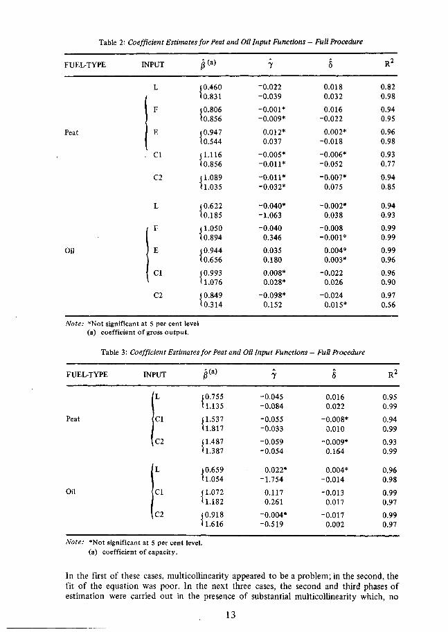
Table 2: Coefficient Estimates for Peat and Oil Input Functions - Full Procedure

FUEL-TYPE

Peat

Oil

INPUT

L

F

E

- Cl

C2

L

F

E

Cl

C2

0(a)

(0.460(0.831

(0.806(0.856

(0.947(0.544

(1.116(0.856

(1.089(1.035

(0.622(0.185

(1.050(0.894

(0.944(0.656

(0.993(1.076

(0.849*0.314

7

"0.022-0.039

-0.001*-0.009*

0.012*0.037

-0.005*-0.011*

-0.011*-0.032*

-0.040*-1.063

-0.0400.346

0.0350.180

0.008*0.028*

-0.098*0.152

5

0.0180.032

0.016-0.022

0.002*-0.018

-0.006*-0.052

-0.007*0.075

-0.002*0.038

-0.008-0.001*

0.004*0.003*

-0.0220.026

-0.0240.015*

R2

0.820.98

0.940.95

0.960.98

0.930.77

0.940.85

0.940.93

0.990.99

0.990.96

0.960.90

0.970.56

Note: *Not significant at 5 per cent level(a) coefficient of gross output.

Table 3: Coefficient Estimates for Peat and Oil Input Functions - Full Procedure

FUEL-TYPE

Peat

Oil

INPUT

L

Cl

C2

L

Cl

C2

0(a>

(0.755(1.135

(1.537(1.817

(1.487(1.387

(0.659(1.054

(1.072h.182(0.918(1.616

7

-0.045-0.084

-0.055-0.033

-0.059-0.054

0.022*-1.754

0.1170.261

-0.004*-0.519

5

0.0160.022

-0.008*0.010

-0.009*0.164

0.004*-0.014

-0.0130.017

-0.0170.002

R2

0.950.99

0.940.99

0.930.99

0.960.98

0.990.97

0.990.97

Note: *Not significant at 5 per cent level,(a) coefficient of capacity.

In the first of these cases, multicollinearity appeared to be a problem; in the second, thefit of the equation was poor. In the next three cases, the second and third phases ofestimation were carried out in the presence of substantial multicollinearity which, no

13

doubt, is the main reason for the unexpectedly high values of the final estimates of 0.In the case of the Komiya formulation, the fit of the equation was poor and the estimatedvalue of |8 insignificantly different from zero at the 5 per cent level as indicated by theasterisk in Table 4.

Table 4: Comparison of Estimates of the Scale (Size) Coefficient pfrom Pooledand Cross-Section Models

INPUT

L

F

E

Cl

C2

MODEL

(a) Independent Variable —

i Pooled Model - (4) [Table 2]( Lau and Tamura — LT

i(4)UT1(4)UT((4)UT((4)UT

PEAT

OUTPUT

0.460.76

0.811.18

0.951.16

1.120.85

1.090.86

(0.83)

(0.86)

(0.54)

(0.86)

(1.04)

OIL

0.62 (0.19)0.57

1.05 (0.89)1.06

0.99 (0.66)0.91

.0.99 (1.08)0.72

0.85 (0.31)0.72

Cl

C2

(b) Independent Variable - CAPACITY

Pooled Model - (5) [Table 1 ] 0.57 0.99Modified Pooled Model - M(5) [Table 3] 0.76 (1.14) 0.66 (1.05)Komiya - K 0.46 0.38

(5) 1.11 1.30M(5) 1.54 (1.82) 1.07 (1.18)

^ K 0.97 0.42*

(5) 1.05 1.33M(5) 1.49 (1.39) 0.92(1.62)

'K 1.00 0.73

*Not significant at 5 per cent level.

Hypothesis Tests and Discussion of ResultsThere is scope for considerable detailed testing and discussion of the results that have

been presented. However, the following comments concentrate on what are consideredto be some of the more substantive matters. First, certain issues which involve the testingof hypotheses about the nature of the entire production structure in thermal electricitygeneration are discussed, namely, the homotheticity of the structure and the nature ofoverall returns to scale and technical change. Second, there is a brief discussion of individualinput functions and of the economic interpretation and implications of their respectiveparameter estimates. Of course, consideration of both of these sets of topics presupposesthat the NHL production function provides some explanation for the Irish data.

The overall explanatory power of each of the models examined in the study wasassessed by means of the omnibus F-test of the null hypothesis, H o , that all of its para-meters are zero. Without exception, H o was rejected at the 5 per cent significance level.In the case of fitted models (5) and (4), which produced the results in Tables 1 and 2respectively - and which are the prime concern of this paper - the rejection was quitedecisive.

Having established that the NHL model does provide an explanation for the ESB data,

14

testing of the hypothesis of homotheticity followed using both the OLS results for model(5) and the GLS results for variant (4). The null hypothesis for this test corresponded tothe homotheticity condition given in Section 4, namely, that the coefficient of output,]3, has the same value for all input functions in a given fuel category. For both sets ofresults, the hypothesis was rejected. In the case of model (5), homotheticity in peat-firedgeneration was rejected rather more decisively than for oil-fired generation. This isreflected in the relatively low value of /3L for peat which, on the basis of the standardtwo-sided t-test of the difference between regression coefficients, is significantly differentfrom the j§ values for all of the other inputs at the 5 percent level. In the oil category,however, j3L is not statistically different from j§F, j8E and j§c at the 5 per cent level. Thereare similar differences in the A values for different inputs, though these were not testedformally.

The rejection of homotheticity is of considerable importance. For a fortiori, homo-geneity of the production structure, and hence overall constant returns to scale - and,indeed, overall increasing and overall decreasing returns to scale of any given degree -must also be rejected automatically. This is not to say, however, that the use of individualinputs may not be subject to constant returns to scale. This matter is considered below.

As can be seen from the prevalence of negative values for 7 and 5 in Tables 1, 2 and 3,there is a suggestion that embodied and disembodied technical progress has influenced theuse of the factors of production in both peat- and oil-fired generation. However, many ofthe estimates are not significantly different from zero, and those that are, are generallysmall. The few larger values of 7 and 6 in the GLS results in Tables 2 and 3 generallyrelate to those equations that have been mentioned as being unsatisfactory. On the basisof the results of models (5) and (4), the null hypothesis of overall zero technical change,and that of neutral technical change, could not in fact be rejected at the 5 per cent level.As with the result on overall constant returns to scale, this finding does not necessarilyimply that technical change has not had an impact on the use of individual inputs duringthe sample period. However, it is a somewhat unexpected result, and will be commentedon again in Section 5.

The explanatory power of the large majority of results for the individual input functionswere also highly significant on the basis of F-tests at the 5 per cent level. For example,in the case of the first OLS regressions for peat in model (5), the computed F valuesranged from 26 to 1082, while the 5 per cent critical value, F^7, is 2.63. In the case ofthe final GLS equations for peat in model (4), they ranged from 76 to 2547. Similar highvalues were recorded for the equations in the oil category. Only two equations fitted thedata poorly; these were referred to at the end of the last subsection.

In considering the individual input results, it is useful to bear in mind that to theextent that the data on independent variables are subject to errors of measurement,parameter estimates may be expected to be biased downwards. Attention was drawn tothe possibility of such errors in the measures of capacity and load factor in the subsectionon data. It may also be useful to distinguish between the 0 values for output and thoseobtained using capacity as an independent variable. In what follows, greater attention isconcentrated on the former, and the ex post interpretation of the production function.Finally, in view of the range of models used, no particular set of point estimates is singledout for special consideration. Rather, the emphasis is placed on the general orders ofmagnitude and mutual consistency of the different estimates of individual parameters. Inprinciple, of course, the estimates obtained from the full GLS procedure are favoured, butuse of the extended data set to obtain them gives rise to certain difficulties of interpre-tation as mentioned in the discussion of the empirical analysis in the previous subsection.

LabourIn model (4), the scale coefficient j§, i.e. the partial elasticity of the quantity of labour

used with respect to gross output, ranges from 0.46 to 0.83 in the case of peat, and 0.19to 0.62 in the case of oil. The values for this coefficient obtained using the Lau andTamura model lie within these ranges. Thus, as all of these values are considerably less

15

than unity, even ignoring the suspiciously low value of |3L = 0.185 for oil, a consistentindication of substantial economies of scale in the use of labour emerges, with the economiesbeing somewhat greater in the case of generation using oil.

The results for the size coefficient, obtained from the models involving capacity, alsoreflect economies of scale. In the case of peat, the range of values of 0 is 0.46 to 0.76 (dis-regarding the suspect GLS estimate) which is very similar to the range for the outputcoefficient. In the oil category, for which the range of 0 values is 0.38 to 0.99, the pictureis less clear. If the Komiya estimate is disregarded, however, the indications are thateconomies in the use of labour with respect to plant size are less pronounced than thosefor the use of labour with respect to output for a given plant size.

The values of the size coefficient for labour obtained by Komiya and Barzel, usingdata for the USA, were 0.50 to 0.60, and 0.63, respectively. While these figures aresimilar to those obtained in this study, it should be noted that they relate to coal and oil

, plants and, in the case of oil, to an earlier sample period.The finding of large economies in the (ex post) use of labour is quite in accord with

prior knowledge and expectations. For after a plant is installed, labour is almost a fixedfactor of production. This fact is vividly reflected in the estimated value of X, the partialelasticity of the quantity of labour used with respect to the degree of capacity utilisation,obtained from model (5). The value of X in the labour function for peat plants is zero,statistically; for oil-fired plants, it is 0.25. These figures compare quite closely with thecorresponding figure of 0.17 reported by Barzel; they mean that plants of equal size,operating at different levels of capacity, do not vary substantially in the amount oflabour used.

The values of the coefficient of embodied technical change, 7, are in almost all casesnegative, but small, as noted earlier. The implication of this is that embodied technicalprogress, or the reduction of the labour requirement in plants of a given size or scale ofoperation, but more recent vintage, has been quite modest on a year by year basis. Overa longer time period, however, the impact of embodied technical change is more notice-able. For example, the GLS estimate of-0.039 for peat plants in model (4) suggests thatthe amount of labour required by a plant installed in, say, 1960 was about 48 per centless than a plant installed in 1950, all other things being equal.16 Both Komiya and Barzelreported similar-sized vintage effects. Of course, when combined with an expansion ofscale, the decline in the labour requirement becomes substantial.

The estimated values of 5, where they are significant, are generally much smaller thanthose for 7, suggesting only slight disembodied technical change. Indeed, in all of thelabour functions in the oil category except the unsatisfactory GLS result in Table 2, thevalue of 5 is not significantly different from zero. This may be interpreted as indicatingno discernible change in labour quality or efficiency over the sample period.

FuelThe partial elasticity of the quantity of fuel used with respect to output, j§, ranges

from 0.81 to 0.86 in the case of peat stations, and from 0.89 to 1.05 in the case of oilplants, using model (4). The GLS estimates in each of these categories are significantlyless than unity on the basis of the standard t-test at the 5 per cent level, unlike theestimates from the Lau and Tamura model which are not significantly different fromunity at the 5 per cent level. Despite the closeness of the different numerical values, thereis therefore some doubt about whether fuel economies accompany higher levels of out-put. If they do, as suggested by the preferred GLS results, they are only slight.

The results for the size coefficient in model (5)— 1.05 and 0.93 for peat and oilplants, respectively — are not significantly different from unity, implying constantreturns to size in the case of both types of station. On the other hand, the load factorcoefficient, X = 0.91, is significantly less than unity in the case of peat plants, suggest-ing, like the GLS estimate of 0 in model (4), that there are slight fuel economies to berealised by increasing output and the level of utilisation of the capacity of peat plants.The X value for oil-fired stations is not significantly different from unity and therefore

16

does not lend similar support to the associated GLS estimate of the output coefficient.The X value is also not significantly different from the size coefficient /3 in model (5),which suggests that there is little to be gained by decomposing output into its capacityand load components in the fuel function for oil stations.

The weight of the evidence would suggest acceptance of the hypothesis of constantreturns to plant size. This result confirms expectations, no doubt. However, it differssomewhat from the findings of both Komiya and Barzel. Komiya estimated the sizecoefficient for fuel to be between 0.80 and 0.85; Barzel estimated it to be 0.89. In bothcases the values were significantly less than unity, although Barzel stated that the impor-tance of the economies implied by his result should not be overestimated (see his example:Barzel 1964, p. 137.)

The technical change coefficients, y and 5, in the fuel input functions are on thewhole smaller than those recorded for the labour input functions. In the case of embodiedtechnical change, i.e. the change in the fuel requirement resulting from different vintagesor qualities of equipment, the significant estimates of y are mainly negative. In the caseof disembodied technical change, which may be interpreted as the change in fuel quality,there are small negative and positive values of 5. Negative values indicate increases, andpositive values indicate decreases in fuel efficiency, respectively. It is not particularlysurprising to have observed both. In his American study, Barzel (1964, p. 139) alsoobserved falls and rises of fuel efficiency over time, of up to 10 per cent.

However, it is not the signs of the technical change coefficients that are of greatestinterest, so much as the general contrast between the sizes of the coefficients in the twofuel categories. For purposes of comparison, the final phase estimate of the fuel functionfor oil stations in Table 2 may be disregarded because, probably due to multicollinearity,it contains an unacceptably large positive value for y. The first phase estimate of thisequation is considered more reliable. Nevertheless, it may be seen that the 7 value for oilplants is still, relatively, very much larger than that for peat plants. The same may be saidabout the 7 values given in Table 1. The indications are that embodied technical progresshas been more significant for oil plants than for peat plants.

For example, consider the significant 7 values for peat and oil plants in Table 1. Thevalue of -0.017 for peat means that the difference in the fuel requirement for plantswhose vintage differs by a decade, is only 18 per cent, whereas the value of-0.057 meansthe corresponding difference for oil plants is about 75 per cent, all other things beingequal. Komiya's conclusion that "the improvement in thermal efficiency can be explainedprimarily by the increase in the scale of production rather than by the shift in the function"may hold in the Irish case for peat, but it does not appear to apply in the case of oil-fired generation.

Energy .The size coefficient for the energy function estimated using model (5) is indicative of

slight diseconomies of scale in the case of peat, the j§ value of 1.236 being significantlygreater than unity. In the case of oil plants, constant returns are indicated as the /3 valueof 0.991 is not significantly different from unity. In contrast, there are very clear indica-tions of economies in the use of energy when both types of plant are operated moreintensively, the partial elasticity with respect to degree of capacity utilisation being of theorder of 0.7 in both cases.

This last feature is reflected in the values of the output coefficient estimated usingmodel (4), although at the first stage of estimation the estimates are only slightly lessthan unity. At the final stage, however, they are markedly less and suggest economiescomparable with those for labour. On the other hand, the estimates obtained using theLau and Tamura model are much closer to unity, with constant returns in the case ofpeat plants and slight economies in the case of oil plants being suggested by hypothesistests at the 5 per cent level.

The values of the vintage and time coefficients for energy in both fuel categories arevery similar to the corresponding coefficients in the fuel input functions, at least in the

17

case of model (5). One may thus be led to very similar conclusions. However, in thecase of energy, it is not as easy to dismiss the GLS result for oil plants as it was in thecase of the^fuel function. There is therefore a conflict between the relatively large positivevalue for 7 given by model (4) and the smaller negative value of model (5). A similarsituation exists for peat plants, although the value of 7 from model (4), though positive,is not nearly so large as that for oil plants. The meaning of positive and negative values ofthese coefficients has already been stated. The same kind of conflict does not arise fromthe estimates of 5. Only one of these is significant at the 5 per cent level, namely, theGLS estimate in the peat category, and this, being negative and small, suggests that therehas been a slight increase in efficiency in the use of energy over time.

Energy functions were not estimated in any of the studies described in Section 3. Asfar as the author is aware, no other basis of comparison for the present estimated energyfunctions exists.

CapitalThe estimates of the coefficient of scale, fi, in those models which incorporate output

as an independent variable are similar for the Cl measure of capital based on the cost ofgenerating equipment only, and the C2 measure based on the total capital cost of plants.In the case of peat stations, the coefficient values range from 0.85 to 1.12, and in the caseof oil plants from 0.72 to 1.08, with neither the 1.12 figure nor the 1.08 figure beingsignificantly greater than unity. The coefficients are particularly close for the alternativecapital measures in the case of the Lau and Tamura formulation of the function. While,on the basis of the results for model (4), constant returns to scale cannot be ruled outfor either type of station, the overriding impression is one of slight economies of scalewith respect to the use of generating equipment and the total capital requirement. Thetotal capital economies appear to be somewhat greater in oil-fired generation than inpeat-fired production.

The same broad consistency between estimates based on the use of the two measuresof capital may be observed in the case of the models which employ capacity as an indepen-dent variable. In these cases, however, the indications are of diseconomies in real capitalrequirements. Values of j§ range from 0.97 to 1.54 for peat stations and 1.07 to 1.30 foroil stations when C1 is the dependent variable; and from 1.0 to 1.49 for peat stations and0.73 to 1.33 for oil stations when C2 is the dependent variable, with the figure of 0.73from the Komiya formulation being the only estimate which is significantly less thanunity at the 5 per cent level. There is some suggestion that the diseconomies are less foroil-fired plants than for peat-fired plants.

Such estimates of the partial elasticity of the real capital cost with respect to size(capacity) of plant are in conflict with expectations. They contrast sharply with the kindof value that would be expected on the basis of certain conventions used in engineeringfields to estimate the capital cost of plants of different sizes. In particular, they differconsiderably from 0.6, the so-called "six-tenths factor" proposed by Chilton(1960) andonce widely used by engineers. They are also greater - and in most cases significantlygreater — than the values of the corresponding parameter estimates obtained by Barzeland Komiya. Barzel's estimate was 0.82, while Komiya's was the range 0.80 to 0.85.These values are much closer to those of the coefficient of gross output obtained usingthe model (4) variant of the capital function in this study.

By contrast the estimates of X, the partial elasticity of the amount of capital servicesused with respect to degree of capacity utilisation, are entirely in accord with expec-tations. When C1 is used as the capital measure in model (5), X is not significantly differentfrom zero in both peat- and oil-fired production. The interpretation of this result is thatessentially the same flow of services is required of generating equipment whether a low ora high level of output is produced. On the other hand, when C2 is used as the measureof capital, X is 0.117 in the case of the capital function for peat plants, and 0.257 in thecase of that for the oil category. Although small, both of these values are significant atthe 5 per cent level and are similar to the value of 0.116 reported by Barzel. Thus, with

18

respect to total capital services, very large economies may be derived from higher levelsof capacity utilisation of peat and oil plants, as was found to be the case with respectto labour.

Finally, the coefficients 7 and 5, relating to technical change, are quite small, as in theother equations. The majority of statistically significant values of 7 are negative, indicatingembodied technical progress. The majority of significant values of 5, however, are positive.While this may seem a rather surprising result, it is noteworthy that Komiya also reportedsimilar small positive shifts in his capital function. Their meaning is that disembodiedtechnical change has been negative, that is, there has been a move over time in the directionof plants of the same size requiring more capital. The implication of the existence ofthese opposite signs is that in certain of the capital functions, embodied and disembodiedtechnical change have had a cancelling rather than a mutually reinforcing impact on theuse of capital.

5. CONCLUDING REMARKS

This study was motivated by an interest in applying a relatively new concept of pro-duction theory to a concrete situation. The concept — the non-homothetic Leontiefproduction function — would appear to be very well suited to application to any industrywhose production process is characterised by limited factor substitutability. The case ofelectricity production at plant level in Ireland was chosen because econometric analysisof production in that industry had not previously been undertaken; because good-qualitydata are readily available for plants in the industry; and because several studies of electricityproduction have been done for other countries and it seemed useful to compare resultsfor Ireland with their findings. It was not the intention to relate the exercise to an examina-tion of any particular policy issue that might confront the ESB. However, as was stated inSection 1, there are several kinds of economic issues on which quantitative informationabout the production process may have a bearing. Some of these issues, and the extentof the practical relevance of the results reported in this paper, are briefly discussed below.But first, the main findings of the analysis are summarised.

The NHL production function for electricity generation was estimated in terms of asystem of derived factor input equations using an econometric methodology based onpooled cross-section and time-series data. The equations appear to fit the data well. Onthe basis of the estimates of the scale parameters, the hypothesis of homotheticity, andhence overall constant returns to scale was rejected. In fact, the results clearly suggestthe existence of increasing returns to scale in electricity production at plant level, withsubstantial economies with respect to the labour and energy inputs, lesser economies withrespect to the capital input, and slight economies with respect to the fuel input. All ofthese results are in accordance with previous findings on thermal electricity productionin other countries. However, the results on the capital input function incorporating capacityas an explanatory variable are at variance with the results of previous studies, and withcertain assumptions used by some engineers in estimating the capital cost of plants ofdifferent sizes. Similarly, there is an unexpected result for peat-fired stations in the energyfunction incorporating capacity, which suggests the possibility of slight diseconomieswith respect to plant size. Both of these findings perhaps warrant further investigation.

The estimates of the parameter associated with capacity utilisation are quite in accordwith expectations, suggesting sizeable increasing returns to labour, energy and capital asthe degree of capacity utilisation of a plant increases, and approximately constant returnswith respect to the use of fuel. In contrast, the impact of embodied and disembodiedtechnical change, as measured by the estimates of the coefficients of plant vintage andtime, was found to be unexpectedly small. Indeed, while in a few cases the reduction inthe quantity of an input required to produce a given level of output is not negligible overa sufficiently long time period, the hypothesis of overall zero technical change could notbe rejected.

Comparing results for the two types of plant examined, the scale economies associated

19

with labour were found to be larger for oil plants than for peat plants. But in general, thedifferences between the estimated parameter values of the production structures of thetwo types of plant were not found to be large.

The results seem to show clearly that the scale effect is probably a far more importantfactor in improving the production efficiency of plants than pure technical change. This isnot to say, of course, that technical change has played only a small part in improvingefficiency; that is patently not the case. Rather, it suggests acceptance of the view, expressedby Komiya (1962, p. 166), that "The fact that it has become possible to build larger andlarger generating units realising the benefit of increasing returns is to be considered as themajor achievement of technological progress in this industry." No doubt such a viewwould be widely accepted amongst those concerned with the operation of the electricitysupply industry in Ireland. Therefore, in providing econometric confirmation of this view,the results may not be without interest for them. It is hoped, however, that the individualnumerical estimates of the actual extent of returns to scale and technical progress —though the first of their kind for Ireland and therefore still somewhat tentative — may beof rather more interest than that. Such knowledge may be useful for its own sake, butmore important, it may have relevance for various factors which the plant operator maywish to take into account in formulating policy. Therefore, in conclusion, some of thepossible applications of the results, and the kinds of policy issue on which they mighthave a bearing, are briefly considered.

Using the estimates of the derived input demand equations, it is possible, of course, togive numerical substance to the underlying production function as specified in equation(2). However, there seems little to be gained from this as information about the natureof the production structure is available directly from the estimated input functions.Therefore it would appear to be potentially much more profitable to examine furtherthe direct use of these equations; but it is also possible to make important indirect use ofthem through the derivation of cost functions. It is not the aim here to undertake asystematic exploration of these possibilities, but simply to suggest and comment on someof them.

Thus, for example, the input equations may be used directly to provide an indicationof the optimal relative factor intensities of plants. Using the notation of Section 3, thesemay be written as XJ/XJ = f^O/iX), i f j , for a given output level from a given type ofplant. In principle, knowledge of optimal factor proportions is clearly a matter of impor-tance for the efficient operation of plants. Similarly, in addition to what has already beeninferred about returns to scale and technical change, individual parameter estimates maybe used to obtain various other measures, such as of the increasing capital intensiveness ofplants. Hence, although a substitution model was not used, the ratio of the scale para-meters for capital and labour, for example, would appear to indicate a significant long-runtrend of substitution of capital for labour. Such considerations as the importance ofreturns to scale and the likely factor bias of technical change may be of some relevancefor planning activities. In particular, they would seem to have some bearing on suchquestions as whether fewer but larger power stations should be constructed even at therisk of increasing vulnerability, and the estimation of future demand for labour.

From the individual input functions, it is a routine task to derive cost equations, givenfactor prices. Therefore the results of this study provide a means of deriving estimates ofthe total operating cost and capital cost of plants of a given fuel-type, which may operateat varying degrees of capacity. Such cost information may be of value in formulatingcapital investment policy. It should be stressed, however, that econometric cost informationwould only be one small ingredient in the investment decision-making process. The actualprocess is, of course, highly complex. It is complicated, for example, by the fact thatbecause the life-span of capital in the industry is so long, optimisation over a substantialperiod of time is required. Faced by uncertain demands and a life of capital of say 20years, an acceptable optimisation procedure would involve that choice of plant which,for a set of exogenous demands, minimises the present value of expected costs. Moreover,the requirements of reserve capacity to meet the problem of "outage", i.e. breakdown

20

and maintenance, the relationship between total capacity and peak load, and tariff policyand revenue considerations, not to mention the recent surge of interest in nuclear genera-tion, would also complicate the process.

Therefore, without wishing to exaggerate their value, the results of econometric pro-duction studies may shed some useful light on various kinds of policy issue. To theextent that the statistical results of this study are accepted, it is hoped that they mightbe of some help in analysing some of the matters that have been referred to, or, at least,that they might be considered a worthwhile basis for further research by those involvedwith the Irish electricity industry.

REFERENCES

BALESTRA, P. and M. NERLOVE, 1966. "Pooling Cross Section and Time Series Data in the Esti-mation of a Dynamic Model: The Demand for Natural Gas", Econometrica, 34, 3, 585-612.

BARZEL, Y., 1964. "The Production Function and Technical Change in the Steam Power Industry",Journal of Political Economy, 72, 2,133-150.

BOOTH, J.L., 1966. Fuel and Power in Ireland: Part II, Electricity and Turf, Economic and SocialResearch Institute, Paper No. 34, Dublin.

CHILTON, C.H., 1960. " 'Six-Tenths Factor' Applies to Complete Plant Costs", in Chilton, C.H. (Ed.),Cost Engineering in Process Industries, New York: McGraw-Hill Book Company.

DESAI, M., 1916. Applied Econometrics, Oxford: Philip Allan Publishers Limited.DESHPANDE, M.V., 1966. Elements of Electrical Power Station Design, London: Pitman.DHRYMES, PJ. and M. KURZ, 1965. "Technology and Scale in Electricity Generation", Econo-

metrica, 32, 3,287-315.ESB INVESTIGATION COMMITTEE, 1972. Report by the E.S.B. Investigation Committee, Dublin,

Stationery Office.ESB Annual Report, Dublin: Electricity Supply Board (various issues).GALATIN, M., 1968. Economies of Scale and Technical Change in Thermal Power Generation,

Amsterdam: North-Holland Publishing Company.HAITOVSKY, Y., 1969. "Multicollinearity in Regression Analysis: Comment", Review of Economics

and Statistics, 51,4,486-489.HALDI, J. and D. WHITCOMB, 1967. "Economies of Scale in Industrial Plants", Journal of Political

Economy, 75, 4, 373-385.Irish Statistical Bulletin, Dublin: Central Statistics Office (various issues).KMENTA, J., 1911. Elements of Econometrics, New York: The Macmillan Company.KOMIYA, R., 1962. "Technological Progress and the Production Function in the United States Steam

Power Industry", Review of Economics and Statistics, 44, 2, pp. 156-166.LAU, L.J. and S. TAMURA, 1972. "Economies of Scale, Technological Progress, and the Nonhomo-

thetic Leontief Production Function: An Application to the Japanese Petrochemical ProcessingIndustry", Journal of Political Economy, 80, 6, pp. 1167-1187.

NEARY, J.P., 1972. "A Multiple-Option Regression Program for use in Econometric Research",E.S.R.I. Memorandum No. 76, Dublin: Economic and Social Research Institute.

NERLOVE, M., 1963. "Returns to Scale in Electricity Supply", in Christ, C.F. et ah, Measurementin Economics: Studies in Mathematical Economics and Econometrics in Memory of Yehuda Grun-feld, Stanford: Stanford University Press, pp. 167-198.

TELSER, L.G., 1964. "Iterative Simultaneous Estimation of Sets of Linear Regressions", Journal ofthe American Statistical Association, 59, 307, pp. 845-862.

ZELLNER, A., 1962. "An efficient Method of Estimating Seemingly Unrelated Regressions and Testsfor Aggregation Bias", Journal of the American Statistical Association, 57, 298, pp. 348-368.

FOOTNOTES

1. In preparing Section 4, I was faced with a dilemma. I was conscious, on the one hand, of thetechnical, though mostly routine, nature of much of the material it contains, and, on the otherhand, of the fairly general nature of the audience. Therefore, at the risk of being somewhattedious to those familiar with the type of econometric approach used, I have dwelt at rathergreater length on the methodology and results than I would have done had the paper been pre-pared for a more specialised audience. I hope I have struck a reasonable balance.

2. For further details see Booth (1966, Part IIA, especially pp. 9-14), and ESB Investigation Com-mittee (1972, Appendix 1, pp. 2-5).

3. Unless stated otherwise, the statistics given in this Section are based on figures contained in theESB Annual Report for the year ended 31st March, 1976.

4. The names of the stations, their locations and technical specifications are given in ESB AnnualReport (1976, Appendix 6, pp. 4041).

21

5. For greater detail see, for example, Deshpande (1966).6. The load factor = total annual KWh./ (installed KW. x total annual hours) x 100 = percentage of

time a plant is utilised during a year, where KWh. stands for kilowatt-hour, the standard unit ofelectricity output, and KW. stands for kilowatt, a unit of capacity.

7. A survey and critique of the studies of Komiya, Barzel, and Dhrymes and Kurz, and others, iscontained in Galatin (1968, Ch. 4). A summary of Komiya's methodology and results is alsoavailable in Desai (1976, pp. 160-167).

8. These properties are discussed and illustrated by Lau and Tamura (1972, pp. 1170-1171).9. A necessary and sufficient condition for overall constant returns to scale (i.e. to plant output)

follows as ft = \ = 1, for all i, which is equivalent to ft = 1, for all i, in model (4).10. The system of input functions developed by Dhrymes and Kurz gave rise to very serious estimation

problems, quite apart from the nature of the disturbances, and these were approached by an"informal" estimation procedure based on the use of two-stage least squares (see Dhrymes andKurz 1964, p. 294, fn. 5). The Zellner method was used by Lau and Tamura (1972, pp. 1179-1180).

11. See also Kmenta (1971, pp. 513-514).12. The source of the price indices was Irish Statistical Bulletin, Central Statistics Office, Dublin

(various issues).13. The practice of presenting a minimum of statistical detail is followed throughout this Section.

Fuller details are available from the author.14. Multicollinearity was tested for by using the X2-test of Haitovsky (1969) at the 5 per cent sig-

nificance level.15. The GLS computer program, and the programs for all intermediate calculations, were written by

the author. The OLS program used was the modified IBM package of Neary (1972). The machineused was the IBM 360 model 44 at Trinity College, Dublin.

16. The natural antilogarithm of (10 x 0.039) = 1.477.

DISCUSSION

A.G. Kelly: I am happy to propose the vote of thanks to Mr. Harrison for his very interest-ing paper, and to express my appreciation of the quality of the work behind this research.

The engineer manager measures the success or failure in economies of scale and technicalchange in power stations under three main headings - efficiency, cost and reliability.

— As proof that the ESB is successful in efficiency of production of electricity, referto the World's Top Ten Power Stations on efficiency (Kelly 1977) where PoolbegStation is fifth in the world and best in Europe; this is despite the small size ofthis station.

— The cost of completed installations is compared with others around the world. Asan example, we have not found a similar station that compared with the 500 MWTarbert B which was completed at £92/KW in 1975/1976. The final cost of theunit of electricity to the consumer is the ultimate measure of "efficiency". Onthis, the ESB compares favourably with other European utilities and has beencheapest on domestic charges over the past decade. This is without the benefitsof interconnection with nearby utilities.

— Reliability of production is compared with other power station units of plant inthe world. An analysis (Kelly 1979) shows that few units of plant attain a loadfactor of over 80 per cent. The ESB has regularly exceeded this figure, e.g., atPoolbeg and Lanesborough B stations.

The overall system load factor is a measure of good planning, design, rates ofcharge, operation and maintenance. The ESB figure is 56 per cent; the USA is49 per cent—but was 57 per cent in 1957 and has gradually deteriorated.With interconnection with GB or N. Ireland (the present connection has beensevered for some years) our figure could be even better. The load factor of a unitof plant is more important than the efficiency of the unit, e.g., for a coal-firedunit operating at 5,000 hrs/year, 2-weeks extra operation per year is equivalent to\Vi per cent on efficiency; to improve Wi per cent on efficiency in design is notpossible but to design for further reliability certainly is practicable.

22

Now for some detailed comments on the actual paper:

Plant Ratings: The USA and UK ratings used are varied from year to year thus yieldingfalse results. The study (Kelly 1979) has corrected for these. All ESB figures are genuine.

Labour: Certainly, the men/MW of plant has decreased rapidly over the years; this willcontinue with further automation. Indeed, the total staff in the ESB is less in 1979 than1971 even though the output is far higher.

The number of persons employed is, on its own, just a measure of the number ofpersons employed.

Capital: No rule of thumb can be used to say that doubling the unit size increases thecost by a certain amount.

There is always an upper limit to size, e.g., the cost of a 5,000 MW single unit is notknown because such a unit cannot be made. The 250 MW units now operating in Irelandwere not possible years ago. Thus, the capital cost rises rapidly as we approach the upperlimit of technological development.

Economies of Scale: Economy of scale disappears (Kelly 1979) below 1,000 MW; theeconomic size of unit is presently in the range 250 to 350 MW.

The study by Mr. Harrison on economy of production by size of power stations usingpeat gives a false result. This is because, for example, Ferbane 90 MW station has smallerunits of plant than Shannonbridge 40 MW station which has a larger unit (40 MW).

Oddly enough, future improvements in efficiency will be on smaller units used in com-bined cycle plants. The cost of construction of such smaller units is also lower — soeconomy of scale is upset.

Load Factor: is assumed by the author to depend only on despatching policy. Unfor-tunately, similar sized units, e.g., 40 MW units in peat stations have not equal reliability;some are excellent and would match the world's best but others are not so excellent. Thisdepends mainly on the design by different manufacturers.

It is axiomatic that production costs reduce with increasing load factor. It is notnecessary to do a statistical study to discover that "with zero load factor, the cost perunit produced is infinite."

Fuel: The efficiency of use of fuel had attained a maximum of 40 per cent (on netcalorific value) and the higher efficiencies were attained in the range of sizes 100 MW-200 MW in Ireland/UK (Kelly 1979). This upper limit to efficiency has existed for manyyears.

However, a new technological development has introduced an improvement. This isthe development of the combined cycle plant such as the new ESB power plant at Marina,Co. Cork. The new limit for efficiency has now quickly risen to over 45 per cent.

The efficiency of production of a 40 MW peat unit is shown by the fact that overallcost of a unit of electricity is only 75 per cent of that from the smaller 20 MW units; yetthe author does not arrive at this conclusion from the statistical study because of the useof total plant rather than units of plant as the basic item examined.

Other investigators (Niebo 1979) attempted to deduce results from statistics of theUSA unit results. The results were mostly statistically inconclusive.

Comment: The data used for Ireland could profitably be compared with a larger poolsuch as the USA, for which all data are available.

This study by the author is a very interesting statistical exercise. The fact that theengineering data and constraints mentioned here are not allowed for, and that thus theconclusions tentatively put forward are often incorrect, does not detract from this.

If the author wished to proceed to correct the study to conform with engineeringrealities, the ESB would be more than pleased to co-operate.

23

REFERENCES

KELLY, A.G., 1977. "World's Top Ten Power Stations for 1975 or Nearest Fiscal Year", Combustion,September 1977, p. 15.

KELLY, A.G., 1979. "Economic Unit Size", Institution of Mechanical Engineers Paper No. C65/79,Proceedings of Conference "Making Steam Plant Pay", Harrogate, England, 1979, pp. 99-107.

NIEBO, R.J., 1979. "Power Plant Productivity Trends and Improvement Possibilities", Combustion,January 1979, pp. 12-21.

Colm McCarthy: Mr. President, Ladies and Gentlemen: It is a pleasure to have the oppor-tunity to second the vote of thanks to Mr. Harrison on this evening's paper. There havebeen only a few production function studies on Irish data and this is the first attempt tomodel the production of electricity. I will confine my remarks to just two areas — theeconometric issues raised by Mr. Harrison's paper, and some of the economic issuesraised by the power generation industry generally.

The log-log formulation of the input demand equations has the implication that Mr.Harrison's no-substitution assumption suppresses variables from a Cobb-Douglas input(factor) demand specification. With Q = f(K,L) in the familiar notation, the Cobb-Douglasfactor demand equations are, for K say, of the form

logK = aQ + a^ogQ + a2logL (1)

while Mr. Harrison's choice of functional form (which is arbitrary) would yield

logK = b0+b1logQ (2)

Thus the force of the Leontief specification is that the demand for each input is indepen-dent of the demands for the other inputs, i.e. that a2 in (1) is zero. It would hardly beinteresting to test for the presence of substitution possibilities in the context of (1), sincethe Cobb-Douglas elasticity of substitution is unity. Such a high figure would be amazingfor the type of productive process described by Mr. Harrison. However, the possibilitythat the elasticity of substitution is non-zero might be worth testing for in a framework,such as CES or its extensions, where it is permitted to take on small values.

The assumption that the units of observation are cost-minimising is not as innocuousas it might appear. If they are not, and this is a problem common to all production studies,there is a kind of identification problem. In the present context it would involve inferring,from the input demand functions, that the I^shaped isoquants were located further fromthe origin than they would be for a plant that truly minimised costs. As with any identi-fication problem, extraneous information will resolve the difficulty. If we knew thatthere was a consistent 10 per cent excess usage of a particular factor, a simple re-scalingwould permit identification of the true relationship describing the technology of produc-tion. But no such simple alternative assumption is available. This problem has consequencesfor the conclusions one may draw about such matters as homotheticity, since any size-related pattern in excess usage of particular factors would interfere with the parameterestimates on which the tests are based.

Mr. Harrison's remark that independent variable errors may bias coefficient estimatestowards zero is well taken, but the prevalence of multicollinearity in his data is notedseveral times. Coefficient estimates tend to explode in the presence of multicollinearityand it is difficult to see what the joint impact of multicollinearity and data-errors might be.

The literature on pooling time-series and cross-sections has tended to concentrate ondeveloping GLS methods to deal with heteroscedasticity — Mr. Harrison's finding is thatautocorrelation may be more important. To the extent that a simplification of the GLSprocedure is desirable and may be necessary for computational feasability, it would beuseful if one could develop some generalisations about the circumstances in which oneor other "disease" is likely to be dominant. If the time series are untrended and the cross-section units of equal size, for example, it might be legitimate to ignore heteroscedasticity

24

altogether.Turning to the economics of power generation generally, and the policy issues which

it raises, there are several areas in which research seems called for. Aside from the workwhich Susan Scott has undertaken recently, and which is highly aggregative, I am notaware of any econometric evidence on electricity demand in Ireland. Both for forecastingand as an aid to pricing policy, it would be desirable to know more in this area.

The construction of the Turlough Hill project could be seen as an attempt to dealwith the peak load problem from the supply side. It would be interesting to contrast theeconomics of a supply-side solution of this problem with those of a demand-side solution,based on peak-load pricing.

A third area of inquiry which may be worthy of attention concerns the choice ofprimary energy sources and of plant sizes in electric power supply. Choice of one energysource and one huge plant might minimise costs under certainty: given the likelihood ofvariation in the relative prices of fuels and the risks of plant shutdowns for technical orindustrial relations reasons, there is a kind of portfolio diversification incentive.

The final item in this arbitrary list concerns the pricing of inputs. There has long beena place on the research agenda for this item given the policy adopted in regard to turf.The decision to use Kinsale gas for electricity generation, and the policy adopted inrelation to the taxation of oil products generally, have made the issue more importantin recent times.

I am aware that the ESB may well have undertaken economic studies in these andother areas for internal consumption, but there has been very little in the public domain.

John W.O'Hagan: I would like to raise three issues resulting both from Mr. Harrison'spaper and from the replies by Mr. Kelly and Mr. McCarthy. The first issue concerns thisproblem of the different meanings assigned by economists and engineers to the wordefficiency. I would like to hear some comment from the engineers present on the ratherrestricted definition of efficiency used in some of Mr. Kelly's charts and I would like toask whether other aspects of efficiency have been looked at in the papers that Mr. Kellyhas mentioned. Second, I wonder if Mr. McCarthy's suggestion of using other CES pro-duction functions, apart from the NHL and Cobb-Douglas functions, could be extendedto include production functions not in the CES class? The last issue I would like to raiseconcerns the use of plant load factor as an explanatory variable in the paper, particularlyin the input demand equations for labour and capital. I find it difficult to envisage how,a priori, there could be any relationship between load factor and the demand for labourand capital and, as such, this variable should not, perhaps, have been included.

May I take this opportunity of warmly associating myself with Mr. Kelly's vote ofthanks to Mr. Harrison. A rather difficult paper, researched with the meticulous care andrigorous standards that we now associate with Mr. Harrison's work, was presented in amost interesting manner.

Patrick Honohan: The difficulty in disentangling the respective effects of scale and tech-nological progress on factor demand is particularly important in this study which, afterall, is focused on exactly these effects. That technological progress seems to have manifesteditself in the availability of larger plant sizes certainly presents an econometric problem. Iwonder whether experimentation with different functional forms, or other representationsof technological progress than those used, might perhaps have allowed for the separateidentification of the two effects.

Reply by MJ. Harrison: I am most grateful to the Society for giving me the opportunityof presenting my paper this evening, and to those who spoke on the paper for theirvarious comments. All but one of the speakers made some points which are not directlyrelated to the subject of the paper. Mr. Kelly's remarks on how engineers assess theefficiency, costs and reliability of electricity production by international comparisonswere interesting and informative. I agree fully with Mr. McCarthy's view that there would

25

seem to be considerable scope for further research into other areas of the economics ofpower generation in Ireland, not least into the demand for electricity; and I sympathisewith Mr. O'Hagan's concern about the engineers' use of the concept of efficiency. In myreply, however, I propose to confine my attention to those points which were directedtowards, or have a bearing on, specific aspects of the paper.

With regard to Mr. Kelly's detailed comments, I am interested and pleased to hear thatthe ESB figures on plant ratings are considered accurate. For this means that my commentson the possible shortcomings of the measures of capacity and degree of capacity utilisationused in the paper are probably unduly pessimistic, and my concern for the associatedbias in parameter estimates largely unwarranted. I am also pleased to hear what Mr. Kellyhad to say about capital cost. In the paper I express some surprise at the values I obtainedfor the coefficient of size in the capital equations, which in almost all cases are greaterthan unity, indicating diseconomies of scale, and greater than the corresponding figuresobtained in the USA. However, given that the American figures were obtained in the1960s, and given what Mr. Kelly has said, the finding now seems less surprising. Presumablythe stations with the 250 MW sets (a 270 MW set in the case of Poolbeg) are using setssufficiently close to the technological limit for unit size, mentioned by Mr. Kelly, for thediseconomies in capital cost to have manifested themselves in my results.

I am very much aware of the problems caused by different generating stations havingdifferent numbers of differently-sized units. Indeed, much of the force of the critique ofproduction studies put forward by Galatin (1968), to which I alluded at the start ofSection 3, was directed at this problem, referred to by Galatin as the "machine-mix"problem. Given the data available to me, however, I was not, as stated in the paper, in aposition to adopt a feasible alternative approach which would make due allowance formachine-mix. Despite this, I am not convinced that my findings on the relative economyof the smaller peat stations is totally fortuitous, as Mr. Kelly's remark on the matterappears to suggest.

I would dispute Mr. Kelly's suggestion that I assume in the paper that load factordepends only on despatching policy. I do say that degree of capacity utilisation is deter-mined essentially by load-despatching policy, but, aware of both forced and planned"outage", I also draw attention in Section 2 to the possibility of breakdown of equipmentand its shut-down for maintenance purposes. Lest Mr. Kelly's unreferenced quotation beascribed to me, I also have to quibble with his other point concerning load factor. First,it may well be "axiomatic" that unit costs decline as load factor increases, just as it is"axiomatic" that in the case of most goods the quantity purchased per unit time decreasesas price increases, ceteris paribus. This, surely, does not make attempts to quantify therates at which these changes take place unnecessary. Second, the statistical study I reportin the paper was not directly concerned with production costs at all, and certainly notwith what is stated in Mr. Kelly's quotation. Incidentally, it is not surprising, therefore,that I do not arrive at the conclusion concerning overall costs of a unit of electricitywhich Mr. Kelly refers to under the heading Fuel. To say that I do not arrive at thisconclusion for the reason stated by Mr. Kelly would seem to me to be a non sequitur,although, as I have already mentioned, I acknowledge the difficulties and implications ofthe machine-mix problem for the achievement of my actual aims as set out in Section 1.

It would be interesting to derive the cost structure implied by my results, of course.As mentioned in Section 5 of the paper, this would not be difficult. Were it to be done,my suspicion is that the resulting ratio of generating costs for a 40 MW peat station tothose of a 20 MW peat station would not be too far out of line with that which Mr. Kellyquotes.

While the paper does contain some comparisons of my results for Ireland with similar,though rather older, results for the USA, I agree with Mr. Kelly that it would be usefulto make comparisons using more recent data on the larger number of American, andperhaps British, power stations. I do not have any immediate plans to refine my studyand/or to carry out such comparisons, but should I return to do more econometric workon electricity production, I should be eager to avail of Mr. Kelly's kind offer of co-

26

operation from the ESB on matters of engineering detail and data provision.Mr. McCarthy began by commenting on my choice of functional form for the input

equations and suggesting that it might be useful to employ some other form to allow forthe possibility of non-zero elasticity of substitution between factors. I have no doubtthat this would be appropriate for a study undertaken at the level of the firm, or at plantlevel if the concern was with the ex ante production function. However, as stated inSection 4 of the paper, I was primarily concerned with the ex post production function.Given the nature of the electricity production process, and the not insubstantial body ofempirical results obtained for other countries using various functional forms, includingthe CES function, I am not sure that substitution models warrant serious considerationas models of the ex post production function, and I remain satisfied with zero substitutionas a maintained hypothesis for the purposes of my study.

Incidentally, while I agree that there is inevitably an element of arbitrariness in thechoice of any functional form for an economic relationship, my choice of log-log was nottotally arbitrary. First, the choice was based on the theoretical rationale of Haldi andWhitcombe (1967) to which I referred in Section 4 of the paper. This rationale is par-ticularly compelling in the case of the capital equation, I feel. For, without going into thedetail of the argument, the relationship between the amount of material required to buildequipment, and the capacity of the equipment, is invariably close to a geometrical one.Second, in many previous studies of electricity production, log-log formulations haveperformed well by comparison with alternative formulations.

In view of these various points concerning functional form, I would want to have verygood reasons before trying other forms in what, otherwise, would be a totally arbitrarymanner. Does Mr. O'Hagan, for example, have strong feelings about why my chosenfunctional form might not be the most appropriate, and has he any specific suggestionsas to what kind of functions, not in the CES class, might constitute a superior alternative?The problem of untangling the effects of scale and technological change on factor utilisationmay well be a good enough reason, as Dr. Honohan suggests. I am not aware of otherfunctional forms having been used in the literature specifically to try to effect thisseparation, nor, I confess, of any potential types of equation that would allow this to beachieved. The matter would, undoubtedly, seem to deserve further consideration.

Mr. McCarthy raises a number of other points which would apply to most econo-metric studies of production. The point about the possibility of X-inefficiency and theassociated problems of identifying the production surface and hence drawing conclusionsabout its precise nature from my parameter estimates is well-taken. Unfortunately, as hesays, there is no easy way of circumventing this problem. I certainly did not have thekind of extraneous information he mentions to resolve the matter. What I did have, how-ever, were statements from the ESB on the basis of which I felt able to use the assumptionof cost-minimisation in the operation of plants as a not too unrealistic approximation.

Mr. McCarthy raised an interesting question concerning the likely consequences of thesimultaneous occurrence of errors in variables and multicollinearity. As far as this study isconcerned, however, it seems from what Mr. Kelly has said about the accuracy of theESB plant capacity figures that errors in variables may be much less of a problem than Ioriginally thought it might have been, as I indicated earlier. Furthermore, I took care tocheck on the incidence of multicollinearity at all stages of estimation; indeed, it will berecalled that I abandoned my first attempt at estimation entirely due to what I consideredan unacceptably high prevalence of the problem. Contrary to what Mr. McCarthy suggests,multicollinearity did not seem to be a problem in obtaining my final estimates. The fewequations in which it was detected in large measure were recorded in Section 4 of thepaper.

I agree with Mr. McCarthy's remark on the potential usefulness of some kind of guide-lines on the likely relative significance of autocorrelation and heteroscedasticity incircumstances in which pooled cross-section and time-series data may be available, if suchguidelines could be devised. It might be the case that heteroscedasticity tends to be slightwhere the cross-section units are of similar size, but the interesting thing about my finding

27

on the matter is that heteroscedasticity was slight, contrary to expectation, in a situationin which the cross-section units were of widely varying sizes. On the other hand the cross-section sample was quite small. I feel that the prospect of being able to ascertain the kindof guidelines Mr. McCarthy envisages is, in fact, remote.

Mr. O'Hagan's point concerning the use of load factor as a variable in the input equationsmight, perhaps, be met by debating the validity of his a priori view of the relationships.For example, it is not obvious to me, particularly in view of what Mr. Kelly has saidabout reliability of plant and the difficulty of achieving high load factors, that it wouldnot require a larger amount of labour to deal with the increased problems of breakdownand servicing that may reasonably be assumed to be associated with the maintenance ofa higher load factor. However, my use of load factor in the labour and capital equationswas not based on a priori considerations so much as statistical expediency; and while itis, I believe, an important variable in the fuel and energy functions - and my resultswould seem to provide confirmation of this - load factor could, I agree, have beenexcluded from the labour and capital functions. But, given the stochastic specification ofthe model, such exclusion would have meant that efficient estimation of individualequations using ordinary least squares would not have been possible. Rather, as mentionedin the paper, efficient estimation would have required Zellner's method for seeminglyunrelated regressions. Not having a readily available computer program for Zellner'smethod, I chose not to exclude load factor essentially in the interests of simple, yetefficient, estimation based on the use of ordinary least squares regression. Incidentally,it transpired that the estimated coefficients of load factor in the labour and capitalequations were all small, as expected, and most were not significantly different fromzero at the 5 per cent probability level.

It is well-known that inclusion of superfluous variables in an equation does not giverise to any bias in the least squares estimates of the parameters. However, it does entailsome cost, of course, namely that the fit of the equation would almost certainly appearbetter than it would be without the additional variables.

In conclusion, I would do no more than reiterate my thanks to all those who con-tributed to the discussion of my paper this evening.

28