JOURNAL OF XX, VOL. X, NO. X, JANUARY XXXX 1

Formal and Compositional Analysis of PowerSystems using Reachable Sets

Matthias Althoff

Abstract—Power system stability analysis becomes more im-portant in the presence of ever increasing variations in operatingconditions. Traditionally, the operation of power systems isverified for specific operating conditions. In this work, thestability analysis is performed for a set of operating conditionsusing reachability analysis, which makes it possible to computethe bounds of all possible system trajectories. Thus, reachabilityanalysis can be used to rigorously check specifications. Contraryto previous work, the presented approach does not requiremodel simplifications when the system is described by semi-explicit, nonlinear, index-1 differential-algebraic equations. Themain obstacle in reachability analysis is the scalability towardslarger systems, which is addressed by investigating compositionaltechniques. As a result, transient stability and variable energyproduction can be analyzed for the IEEE 14-bus and 30-busbenchmark systems, for which the computation times are ordersof magnitude faster than the simulation of all cases starting inthe corners of the set of possible initial states.

Index Terms—Reachability analysis, stability analysis, com-positional analysis, power systems, transient stability analysis,uncertain energy production, differential-algebraic equations,formal verification.

I. I NTRODUCTION

The ongoing trend towards decentralized power generationwith a considerable share of renewable energy sources resultsin a less predictable operation of power systems. New anal-ysis techniques are required to consider all possible futurebehaviors to ensure a reliable operation of power systems.In this paper, reachability analysis is proposed as a formaltechnique to verify if specifications are met under uncertainoperating conditions. Reachability analysis computes theset ofall possible (infinitely many) trajectories of a dynamic modelwhen the uncertainty of initial states, time-varying inputs, andparameters is bounded by sets.

This work focuses on large deviations from the initial oper-ating condition, such that small-signal analysis techniques canno longer be applied [1, Chap. 12]. The dominant technique inpower systems for model-based analysis of large disturbancesis numerical simulation, which is easy to implement, butcan only provide satisfying results when the actual operatingcondition is known and there are no parametric and inputuncertainties. The knowledge of the actual operating conditionrequires constant simulation of the system for a set of probablecontingencies when new SCADA (Supervisory Control AndData Acquisition) measurements are available at a cycle timeof around 10-30 minutes [2]. Due to increasingly varying

Matthias Althoff is with the Department of Computer Science,Technische Universitat Munchen, 85748 Garching, Germany, email:althoff@tum.de

Manuscript received month day, year; revised month day, year.

operating conditions, the measurements at the last cycle mighthave considerably drifted. In order to rigorously considerthosedrifts, one has to assume a set of possible initial states coveringchanges between SCADA updates. However, the number ofrequired simulations grows exponentially with the numberof state, input, and parametric variables due to a necessarygridding of the multidimensional set bounding all variables.Besides the exponential complexity, numerical simulationisnot a formal technique, i.e., one cannot certify whether theeffect of a control action complies with the system specifica-tion: 1) it does not show that all states (infinitely many) ofan initial set return to the operating point, and 2) it is unclearfor how long a simulation has to be run until a particulartrajectory can be considered stable. The aforementioned issuesare alleviated by faster simulation using parallel-in-space [3]–[5] and parallel-in-time algorithms [6] and by Monte Carlosimulation [7]–[9] to address uncertain prediction.

Instead of explicitly simulating the behavior for stabilityanalysis, direct methods compute regions in the state spacefrom which the system state returns to the original operatingpoint [10]–[12]. Those regions are essential to quickly checkif control actions are capable of stabilizing the system withoutrequiring time-consuming simulations. Direct methods requireLyapunov functions, which can only be found for simplifiedsystem dynamics using network preserving and network reduc-tion methods, where the latter is the dominant technique, seee.g. [10]–[15]. While network preserving methods work withordinary differential equations (ODEs), network preservingmethods use more general models described by differential-algebraic equations (DAEs) [16]–[19]. A challenge for bothisto find the so-calledcritical value of the Lyapunov functionto underapproximate the region of attraction. Especially forsystems with several generators, the critical value is ratherconservative, resulting in an underapproximation of the regionof attraction [10], [11]. Another disadvantages of direct meth-ods is that one cannot check if phase, voltage, and frequencyconstraints are met since direct methods only analyze if asteady state of a disturbed system is eventually reached.

Reachability analysis is a complementary analysis techniquebesides simulation techniques and direct methods. Differingfrom simulation techniques, reachability analysis can provewhether system specifications are fulfilled in the presence ofuncertainties, such as uncertain initial states and uncertaininputs/disturbances. Direct methods are a formal techniquesince they can guarantee stability when the initial state startsin the computed region of attraction. However, other thanreachability analysis, direct methods cannot formally verifywhether constraints are met (e.g. whether frequencies and volt-ages remain within permitted ranges). Since formal analysis of

JOURNAL OF XX, VOL. X, NO. X, JANUARY XXXX 2

the nonlinear dynamics of power systems is undecidable [20],one cannot compute exact reachable sets for this system class,requiring instead the computation of an overapproximationofthe reachable set, which includes all behaviors of the modeledsystem. However, when the overapproximation is too large,one might not be able to verify the system although allspecifications are met in reality. General literature reviews onreachability analysis of dynamic systems can be found in [21]–[24]. Most previous work on reachability analysis in powersystems has been limited to small problems due to the initialcomputational costs of first attempts. In [25], [26], reachabilityanalysis is performed for a single-machine-infinite-bus systemmodeled by ordinary differential equations with only2 statevariables. A slightly larger double-machine-infinite-bussystemwith 2 buses described by ODEs resulting in5 state variables isconsidered in [27], where simulations are performed to approx-imate the reachable set resulting in a non-formal approach,i.e.one cannot prove that the controller meets the specificationsunder all eventualities. A 3-bus system is considered in [28] toinvestigate effects on wind variability. More recent work of thesame authors considers the effects of wind variability for the39-bus New England system model [29] and similar studieson the effect of uncertain energy production on frequencydeviation are studied in [30] for a reduced-order model ofthe U.S. power system. The computations in [28]–[30] aresimplified by linearizing the system dynamics so that theresults are not overapproximative anymore and thus do notqualify for formal analysis.

To the best knowledge of the author, none of the previousmethods for reachability analysis of power systems considersthe original DAE system arising in power system modeling,instead relying on simplification of the system dynamics toordinary differential equations. In the previous work of theauthor [31], a new method is presented which can computethe reachable set of the original DAE systems. The approachproposed in [31] has a complexity ofO(n5), where n isthe number of state variables. Although the complexity ispolynomial, the analysis of large systems results in enormouscomputational costs. In this work, the computational costsaredrastically reduced by investigating compositional techniques,making it possible to compute reachable sets of the IEEE 30-bus benchmark system in less time compared to the IEEE14-bus version when no compositional techniques are ap-plied. Another extension compared to [31] and other previousworks is the investigation of the effect of uncertain energyproduction–not only on frequency, but also on bus voltage andphase under consideration of nonlinear effects.

II. PROBLEM FORMULATION

We consider power systems that can be modeled as a setof semi-explicit, nonlinear, index-1 DAEs, which applies toalmost all power systems (see e.g. [32]). For brevity of the pre-sentation it is assumed that the parameters of the power systemare known and constant over time, resulting in a set of time-invariant DAEs. Extensions required for uncertain parametersare presented in [33]. The vectors of differential variables,algebraic variables, and inputs are respectively denoted by

x ∈ Rnd , y ∈ Rna , andu ∈ Rm, wherend, na, andm are thecorresponding numbers of variables. For a set of consistentinitial statesR(0) and a set of possible inputs/disturbancesU ,the system equations are

x = f(x(t), y(t), u(t)),

0 = g(x(t), y(t), u(t)),(1)

where[xT (0), yT (0)]T ∈ R(0), u(t) ∈ U . The initial state isconsistent wheng(x(0), y(0), u(0)) = 0 and it is assumedthat (1) has a unique solutionγ(t, x(0), y(0), u(·)) for allconsistent initial statesx(0), y(0) and all piecewise continuousinput trajectoriesu(·), where u(t) refers to an input at aspecific point in timet. No other assumption besides uniquesolutions are required. The goal of this work is to computethe reachable setRe([0, tf ]) of (1) for a time interval[0, tf ]:

Re([0, tf ]) ={

γ(t, x(0), y(0), u(·))∣∣∣[xT (0), yT (0)]T ∈ R(0),

{

u(t) ∈ U , t ∈ [0, tf ]}

.

The superscripte on Re([0, tf ]) denotes the exact reachableset, which cannot be computed for nonlinear DAE systems asmentioned in the introduction [20]. For this reason, algorithmsare presented which compute as tight as possible overap-proximationsR([0, tf ]) ⊇ Re([0, tf ]). For simplification, theexpressionreachable setis used even whenoverapproximativereachable setsare computed. For later derivations, the projec-tion of the reachable set onto the coordinates of differentialvariables is denoted byRd([0, tf ]) and onto the algebraic vari-ables byRa([0, tf ]). Since reachable sets contain the union ofall possible simulations, the same types of analysis performedwith simulations can be performed with reachable sets. Notethat reachability can in principle also be applied to chaoticsystems [34]. In this work, the focus is on transient stabilityanalysis and the effects of uncertain energy production.

III. PRELIMINARIES

The presented approach is based on known techniquesfor computing reachable sets of linear differential inclusions,which are recapitulated in this section. Reachable set computa-tions are typically performed iteratively for short time intervals

τk := [tk, tk+1].

In this work, constant-size time intervalstk := k r are used tofocus on the main innovations, wherek ∈ N is the time stepandr ∈ R+ is referred to as the time increment. An extensionto variable time increments is described in [35].

The iterative computation of reachable sets for linearsystems requires set-based addition orMinkowski addition(X⊕Y := {x+y|x ∈ X , y ∈ Y}) and set-based multiplication(X ⊗ Y := {x y|x ∈ X , y ∈ Y}). Note that the symbolfor set-based multiplication is often omitted for simplicity ofnotation, and that one or both operands can be singletons. Abrief description of the main steps for obtaining reachablesetsfor a single time interval is provided below.

In this section, the reachability analysis of linear differentialinclusion ˙x ∈ Ax(t) ⊕ U is recapitulated, wherex ∈ Rnd ,A ∈ Rnd×nd , and U ⊂ Rnd is a set of uncertain inputs. A

JOURNAL OF XX, VOL. X, NO. X, JANUARY XXXX 3

tilde is used for the variables of the linear differential inclusionto distinguish the variables from the ones of the originalnonlinear DAEs. For further computations, some variables andsets are introduced:uc is the center ofU , U∆ := U ⊕ (−uc)is the deviation ofU from the centeruc, the reachable set ofthe affine dynamics ˙x = Ax(t) + uc is Rd

a(t), the reachableset of the particular solution due to the uncertain inputU∆ isRd

p(U∆, t), and the partial reachable set correcting the initialassumption that trajectories are straight lines betweentk andtk+1 is Rd

ǫ . According to [23], the reachable set for a timeinterval τk is computed as shown in Fig. 1:

1) Starting fromRd(tk), compute the set of all solutionsRd

a(tk+1) for the affine dynamics ˙x = Ax(t) + uc attime tk+1.

2) Obtain the convex hull ofRd(tk) and Rda(tk+1) to

approximate the reachable set for the time intervalτk.3) ComputeRd(τk) by considering uncertain inputs by

addingRdp(U∆, r) and accounting for the curvature of

trajectories by addingRdǫ .

Rd(tk)

Rda(tk+1)

convex hull ofRd(tk), Rd

a(tk+1)

Rd(τk)

➀ ➁ ➂

enlarge-ment

Fig. 1. Steps for computing the reachable set for a linear system.

Using r = tk+1 − tk, the solution ofRda(tk+1) is

Rda(tk+1) = eArRd(tk) +

∫ r

0

eA(r−t) dt uc

︸ ︷︷ ︸

=:xp(r)

,

wherexp(r) is bounded by integrating the finite Taylor serieseAr =

∑ηi=0(Ar)i/(i!) up to orderη to which the remainder

Ep(r) is added:

xp(r) ∈( η∑

i=0

Airi+1

(i+ 1)!⊕ Ep(r)

)

︸ ︷︷ ︸

=:Γ(r)

uc.

The remainder can be overapproximated by an interval matrixEp(r) := [−W (r) r,W (r) r], i.e., by a matrix with lowerand upper bounds on each element, whereW (r) = e|A|r −∑η

i=0|A|iri

i! . For later derivations,W (r) := W (r)r is alsointroduced. The required enlargement of the convex hull (see3rd step in Fig. 1) is achieved by addingRd

ǫ to account forthe curvature of trajectories fromRd(tk) to Rd

a(tk+1) (see[23]) and by adding the reachable setRd

p(U∆, r) due to theuncertain and convex input setU∆ (see [36]):

Rdǫ :=

(F ⊗Rd(tk)

)⊕(F ⊗ uc

)

Rdp(U∆, r) :=

η⊕

i=0

(

Ai ri+1

(i + 1)!U∆

)

⊕([−W (r), W (r)] ⊗ |U∆|

),

with

F :=

(η⊕

i=2

[(

i−ii−1 − i

−1

i−1

)

ri, 0] Ai

i!

)

⊕ [−W (r),W (r)]

F :=

(η+1⊕

i=2

[(

i−ii−1 − i

−1

i−1

)

ri, 0] Ai−1

i!

)

⊕ [−W (r), W (r)].

The absolute value|U∆|i := sup{|ui|∣∣u ∈ U∆

}is defined

elementwise. The reachable sets for the next point in time andtime interval are obtained by combining all previous results(see [36]):

Rd(tk+1) :=eArRd(tk)⊕ Γ(r)uc ⊕Rdp(U∆, r),

Rd(τk) :=CH(Rd(tk), e

ArRd(tk)⊕ Γ(r)uc

)

⊕Rdǫ ⊕Rd

p(U∆, r),

(2)

whereCH() returns the convex hull. Throughout this work,zonotopes are used to represent the reachable sets. How-ever, the proposed algorithms and computations apply to allkinds of set representations. Zonotopes are used since theycan efficiently represent reachable sets in high-dimensionalspaces while operations required for reachability analysis canefficiently be applied to them. Details on the definition ofzonotopes and operations on them are described in Sec. VI.

IV. REACHABILITY ANALYSIS OF NONLINEAR DAESYSTEMS

Other than for linear systems, no closed-form solutionexists for general nonlinear DAEs. In order to exploit theefficient methods of the previous section based on the closed-form solution of linear systems, an abstraction of the originalnonlinear DAEs to linear differential inclusions is performedfor each consecutive time intervalτk. The linear differentialinclusions are computed such that the resulting abstractionis strictly overapproximative, i.e. it contains all behaviors ofthe original dynamics. By re-computing the abstraction foreach time interval, the overapproximation remains small andaccurate results are obtained while traversing the nonlinearstate space far away from the original operating point.

A. Abstraction to Linear Differential Inclusions

The abstraction of the nonlinear DAEs to linear differentialinclusions is based on linearizing the system dynamics andadding the linearization errors as uncertain input. For a concisenotation, the vectorz := [xT , yT , uT ]T , the linearizationpoint z∗ := [x∗T , y∗T , u∗T ]T , and Rz := R(τk) × U areintroduced. To efficiently obtain a suitable linearizationpoint,the volumetric centerscd, ca, cu of the setsRd(tk), Ra(tk),and U , are introduced. In a previous work it is shown thatthe center of the reachable set of the current time intervalis the best linearization point when the linearization error iscomputed via an evaluation of the Lagrange remainder usingbounds on absolute values [33, Prop. 2]. Although a refinedtechnique is used for the linearization error computation inthis work, the center of the reachable set remains the bestchoice for the linearization error. To circumvent the problem

JOURNAL OF XX, VOL. X, NO. X, JANUARY XXXX 4

that the reachable set is required for an optimal lineariza-tion point, which in turn is required for the computation ofthe reachable set, the center of the differential variablesisapproximated by a one-step Euler integration. This yieldsx∗ = cd + 0.5r · f(cd, ca, cu), where the step size is0.5rbecause the center of the reachable setRd(τk) for the timeinterval τk is expected to be reached after half the intervalduration of tk+1 − tk = r from the centercd of Rd(tk).Besides the linearization point of the dynamic variables, thelinearization point of the inputs is chosen asu∗ = cu andthe linearization point of the algebraic part is computed suchthat it is consistent with the constraint0 = g(x∗, y∗, u∗)using the Newton-Raphson method. The linearization of theoriginal dynamics in (1) is performed using a first-order Taylorexpansion with Lagrangian remainder:

xi = fi(z(t)) ∈ fi(z∗) +

∂fi(z)

∂z

∣∣∣z=z∗

(z(t)− z∗)

⊕

{1

2(z(t)− z∗)T

∂2fi(z)

∂z2

∣∣∣z=ξ

(z(t)− z∗)

∣∣∣∣ξ, z(t) ∈ Rz

}

︸ ︷︷ ︸

=:Ldi

,

0 = gj(z(t)) ∈ gj(z∗) +

∂gj(z)

∂z

∣∣∣z=z∗

(z(t)− z∗)

⊕

{1

2(z(t)− z∗)T

∂2gj(z)

∂z2

∣∣∣z=ξ

(z(t)− z∗)

∣∣∣∣ξ, z(t) ∈ Rz

}

︸ ︷︷ ︸

=:Laj

,

(3)

whereLdi denotes the projection ofLd onto theith coordinate.

The Lagrangian remaindersLd and La enclose all higher-order terms ifz∗, ξ, z(t) ∈ Rz [37, p. 87]. For subsequentderivations, it is required to separate the effects from differ-ential variables, algebraic variables, and inputs. Therefor, thefollowing sub-matrices of the Jacobians are introduced:

∂f(z)

∂z

∣∣∣z=z∗

= [A, C, B],∂g(z)

∂z

∣∣∣z=z∗

= [D, F, E], (4)

where A ∈ Rnd×nd , B ∈ Rnd×m, C ∈ Rnd×na , D ∈Rna×nd , E ∈ Rna×m, F ∈ Rna×na , and nd, na,m arethe number of differential, algebraic, and input variables,respectively. Inserting the abbreviationz = [xT , yT , uT ]T

and the matricesA-F into (3), and introducingHd,(i)(ξ) :=∂2fi(z)∂z2 )

∣∣z=ξ

, Ha,(j)(ξ) :=∂2gj(z)∂z2 )

∣∣z=ξ

, Rz∆ := Rz ⊕ (−z∗),

ν(t) := z(t)− z∗, yields

x ∈f(z∗) +A(x(t) − x∗

︸ ︷︷ ︸

=:∆x(t)

) +B(u(t)− u∗

︸ ︷︷ ︸

=:∆u(t)

) + C(y(t)− y∗︸ ︷︷ ︸

=:∆y(t)

)

⊕{1

2σ∣∣∣σi = νTHd,(i)(ξ)ν, ξ ∈ Rz , ν ∈ Rz

∆

}

, (5)

0 ∈g(z∗) +D(x(t) − x∗

︸ ︷︷ ︸

=:∆x(t)

) + E(u(t)− u∗

︸ ︷︷ ︸

=:∆u(t)

) + F (y(t)− y∗︸ ︷︷ ︸

=:∆y(t)

)

⊕{1

2φ∣∣∣φj = νTHa,(j)(ξ)ν, ξ ∈ Rz , ν ∈ Rz

∆

}

. (6)

Note thatF is invertible because of the index-1 property, sothat one can reformulate (6) to

∆y(t) ∈ −F−1(

g(z∗) +D∆x(t) + E∆u(t))

(7)

⊕{

−1

2F−1φ

∣∣∣φj = νTHa,(j)(ξ)ν, ξ ∈ Rz , ν ∈ Rz

∆

}

.

Inserting (7) into (5) results in a differential inclusion

x ∈f(z∗) +A∆x(t) +B∆u(t)

− CF−1(g(z∗) +D∆x(t) + E∆u(t)

)⊕ L

=(w + A∆x(t) + B∆u(t))⊕ L,

(8)

where

w := f(z∗)− CF−1g(z∗), (9)

A := A− CF−1D, B := B − CF−1E,

and

L ={1

2(σ − CF−1φ)

∣∣∣σi = νTHd,(i)(ξ)ν,

φj = νTHa,(j)(ξ)ν, ξ ∈ Rz , ν ∈ Rz∆

}

.(10)

One can further simplify (8) by combining the singletonwand the setsB(U ⊕ (−u∗)) andL to a new setU :

˙x ∈ Ax(t)⊕ U , (11)

x(t) := ∆x(t), U := w ⊕ B(U ⊕ (−u∗)) ⊕ L.

The obtained differential inclusion can be solved as describedin Sec. III. Still remaining is the determination of linearizationerrors.

B. Computation of the Linearization Error

The problem with evaluating (11) is that the set of lin-earization errorsL is not known in advance, consequentlyUis unknown, as well. As an initial guess the most recentlycomputed linearization errorL is enlarged by a user-definedfactorλL ∈ R+ around the volumetric centercL of L:

L = cL ⊕ λL(L ⊕ (−cL)). (12)

In the event that the enclosure assumption (L ⊇ L) is notcorrect after computing the reachable set and the associatedset of linearization errors,L has to be further enlarged. Inorder to bound the set of linearization errors, one additionallychecks ifL ⊆ Lmax, whereLmax is set by the user. If theabove inclusion is not fulfilled, the reachable set has to be splitin order to reduce the linearization error or the time incrementr has to be reduced.

The set of linearization errorsL is computed based on thereachable setRd(τk) of the linear differential inclusion (11)after replacing the input setU by U = w⊕B(U⊕(−u∗))⊕L,which considers the linearization error assumptionL insteadof L. After applying the procedures in Sec. III on the lineardifferential inclusion (11), one obtains the reachable setofthe differential variablesRd(τk). For computing the set oflinearization errors, the reachable set of the differential andalgebraic variables is required, which can be solely recon-structed by the reachable set of the differential variables. This

JOURNAL OF XX, VOL. X, NO. X, JANUARY XXXX 5

is achieved by firstly starting withx(t) = x∗ + ∆x(t) andy(t) = y∗ + ∆y(t), secondly replacing∆y(t) with (7), andthirdly substituting specific values by sets:

R(τk) =

[x∗

y∗ − F−1g(z∗)

]

⊕

[I

−F−1D

]

(Rd(τk)− x∗)

⊕

[0

−F−1E

]

(U − u∗)⊕

[0

−F−1

]

La.

(13)

The reachable setR(τk) is used to compute the set oflinearization errorsL as presented in [31]. The computa-tion of the linearization error is the bottleneck in terms ofcomputational costs of the presented approach. When usingzonotopes as a set representation, all operations requiredfor the reachability analysis excluding the linearizationerrorcomputation have complexityO(n3), wheren is the numberof dynamic and algebraic variables. The linearization errorcomputation, however, has complexityO(n5). For this rea-son, compositional techniques are investigated to scale theapproach to larger power systems as presented in the nextsection. The overall algorithm of all previously mentionedsteps is presented in Alg. 1.

Algorithm 1 reachNext(Rd(tk),L,U , A, B, w, r,Lmax, λL)

Require: Previous setRd(tk), previous linearization errorL, input setU , linearized system matrixA, linearizedinput matrixB, constant inputw, time incrementr, max.linearization errorLmax, factorλL

Ensure: Rd(tk+1),R(τk), split1: repeat2: L = cL ⊕ λL(L ⊕ (−cL)) (see (12))3: U = w ⊕ B(U ⊕ (−u∗))⊕ L (see (11))4: computeRd(τk) using (2) based onU5: computeR(τk) using (13)6: computeL by evaluating (10) according to [31]7: until L ⊆ L ∨ L * Lmax

8: if L * Lmax then9: split = true

10: else11: split = false12: U = w ⊕ B(U ⊕ (−u∗))⊕ L (see (11))13: computeRd(tk+1)using (2) based onU14: end if

V. COMPOSITIONAL REACHABLE SET COMPUTATION

In order to improve the scalability of the proposed reacha-bility analysis, two compositional techniques are investigated.One of them is to split the power grid into subsystems forwhich the reachable set is computed separately. The othertechnique compositionally computes the set of linearizationerrors, while abstracting the dynamics to linear differentialinclusions using the full model.

Before applying compositional analysis techniques, one hasto partition the power system into subsystems. Partitioningof power systems is a well-known problem for differentaspects of power systems. Examples include coherency-based

decomposition [38], [39] and graph-based decomposition [40].Since this work focuses on the compositional computationof reachable sets for a given partition, we assume that areasonable partition is already provided, where transmissionlines are the interfaces. Since the transmission lines are thesubsystem interfaces, the bus phase angles and the bus voltageare internal variables when the bus is within the subsystem,and a system input otherwise. The assignment of the variablesto the dynamic and algebraic state vectorsx, y as well as tothe input vectoru are described in Sec. VII-A.

A. Compositional Reachable Set Computation

This subsection describes the first option investigated forcompositional analysis by splitting the power system intosubsystems. The reachable set of each subsystem is computedas presented in Alg. 1. The input sets representing inputs tothecomplete system are known, however, the input sets originat-ing from the interfaces of the subsystem are unknown. Theydepend on the reachable set of neighboring subsystems, whichin turn depend on the reachable sets of other subsystems.The basic idea for breaking this mutual dependence apart issimilar to the computation of the linearization error. First, theinterface inputs of theith subsystems are enlarged by a factorλU (analogously to (12))

U (i) = c(i)U ⊕ ((λU − 1)Λ(i) + I)(U (i) ⊕ (−c

(i)U )), (14)

whereΛ is a diagonal matrix that contains ones for indicescorresponding to interface inputs and zeros otherwise. Basedon the system inputU (i), the reachable set of the corre-sponding subsystem is computed as presented in Alg. 1. Foraggregating the reachable sets of the complete system bypartial reachable setsR(i)(τk) of the ith subsystem, matricesΦ(i) are introduced, which map the local states of theith

subsystem to the states of the full system. The matricesΦ(i)

contain ones when states are correlated, and zeros otherwise,so that the complete reachable set is obtained using theCartesian product:

R(τk) = Φ(1)R(1)(τk)×Φ(2)R(2)(τk)×. . .×Φ(ns)R(ns)(τk),(15)

wherens is the number of subsystems and the computation oflinear maps and Cartesian products of zonotopes is performedas presented in Sec. VI. In order to check if the assumption onthe set of interface inputs is correct for all subsystems, furthermatricesΥ(i) are introduced, which map the states of thecomplete system to the interface inputs of theith subsystem.Again, the matrix contains ones for corresponding states andinterface inputs and zeros otherwise. If

∀i : Υ(i)R(τk) ⊆ Λ(i)U (i)

the assumption is overapproximative and thus valid. Other-wise, one has to re-apply the enlargement in (14) for thesubsystems that violate the assumption. This procedure issummarized in Alg. 2 under the assumption that no split isrequired.

JOURNAL OF XX, VOL. X, NO. X, JANUARY XXXX 6

Algorithm 2 reachNextCompositional(R(i),d(tk), λU ,U(i),

otherInputsToReachNext)

Require: Previous setR(i),d(tk) and input setU (i) for eachsubsystem, factorλU , otherInputsToReachNext).

Ensure: R(i),d(tk+1),R(τk)1: ∀i : inputEnclosure(i) = false

2: repeat3: for i = 1 . . . ns do4: if inputEnclosure(i) == false then5: obtain U (i) based onU (i) using (14)6: Alg. 1 based onU (i) → R(i),d(tk+1),R

(i)(τk)7: end if8: end for9: R(τk) = Φ(1)R(1)(τk)× . . .× Φ(ns)R(ns)(τk)

10: for i = 1 . . . ns do11: if Υ(i)R(τk) ⊆ Λ(i)U (i) then12: inputEnclosure(i) = true

13: else14: inputEnclosure(i) = false

15: end if16: U (i) = Λ(i)U (i) ⊕ (I − Λ(i))U (i)

17: end for18: until ∀i : inputEnclosure(i) == true

B. Compositional Linearization Error Computation

In some power systems, generators might be strongly cor-related, resulting in unsatisfactory overapproximationsof thecompositional algorithm in Alg. 2. Since most of the compu-tation time is spent on evaluating the linearization error,onecould only compute the linearization error compositionally,while maintaining all the correlations for the reachable setcomputation in Alg. 1.

Using a decomposition of the full system into subsystemsas in the previous subsection, the Lagrangian remainder in(10) is evaluated compositionally. For this purpose, the set ofinput values from subsystem interfaces has to be consideredresulting in the set of inputs for each subsystem as proposedin (14). The partial Lagrange remainders of theith subsystemdenoted byL(i) are combined to the complete Lagrangeremainder as for the reachable set in (15):

L(τk) = Φ(1)L(1)(τk)×Φ(2)L(2)(τk)× . . .×Φ(ns)L(ns)(τk).

As previously mentioned, the Lagrange remainder has com-plexity O(n5), where n is the number of state variables,whereas all other operations have complexityO(n3) whenusing zonotopes as the set representation. Thus, the com-positional computation of the linearization error has similarcomputational savings than the completely compositional com-putation as presented in the previous subsection.

VI. SET REPRESENTATION BYZONOTOPES

So far, all set-based computations have been introducedindependently of the set representation so that all kinds ofset representations can be used in principle. Typical set repre-sentations are: polytopes [41], zonotopes [42], ellipsoids [43],

support functions [44], and oriented hyperrectangles [45]. Asshown in Sec. III, the set operations required for reachabilityanalysis of linear systems are matrix and interval matrix mul-tiplication, Minkowski addition, absolute value computation,and convex hull. All of these can be efficiently computedusing zonotopes, which makes zonotopes very attractive forreachability computations of linear systems [42], [46].

Definition VI.1 (Zonotope) Given a centerc ∈ Rn and so-called generatorsg(i) ∈ Rn, a zonotope is defined as

Z :={

x ∈ Rn∣∣∣x = c+

p∑

i=1

βig(i), βi ∈ [−1, 1]

}

We write in shortZ = (c, g(1), . . . , g(p)) and define the orderof a zonotope asρ := p

n, wherep is the number of generators.

A zonotope can be seen as the Minkowski addition of linesegments[−1, 1]g(i), which provides an intuition of how azonotope is constructed as presented in Fig. 2.

c

g(1) g(2) g(3)

c⊕ g(1) c⊕ g(1) ⊕ g(2) c⊕ g(1) ⊕ g(2) ⊕ g(3)

constructiondirection

”⊕””⊕”

Fig. 2. Step-by-step construction of a two-dimensional zonotope.

The multiplication with a matrixM ∈ Ro×n and theMinkowski addition of two zonotopesZ1 = (c, g(1), . . .,g(p1)) andZ2 = (d, h(1), . . ., h(p2)), are a direct consequenceof the zonotope definition (see [47]):

Z1 ⊕Z2 = (c+ d, g(1), . . . , g(p1), h(1), . . . , h(p2))

M ⊗Z1 = (M c,M g(1), . . . ,M g(p1))(16)

Additionally, the convex hull ofZ1 andeArZ1 is required (see[46]):

CH(Z1, eArZ1) ⊆

1

2(c1 + eArc1, g

(1) + eArg(1), . . . , g(p1) + eArg(p1),

c1 − eArc1, g(1) − eArg(1), . . . , g(p1) − eArg(p1)).

(17)

After introducing the matrix of generatorsG =[g(1), . . . , g(p)

]and the alternative notation of a zonotope by

Z = (c,G), the Cartesian product of two zonotopesZ1 = (c,G) andZ2 = (d, H) is

Z1 ×Z2 =

([cd

]

,

[G 0

0 H

])

,

where0 is a matrix of zeros of proper dimension. For themultiplication of an interval matrixM with a zonotope, thematrix M is split into a real-valued matrixM ∈ Rn×n andan interval matrix with radiusS ∈ Rn×n, such thatM =

JOURNAL OF XX, VOL. X, NO. X, JANUARY XXXX 7

M ⊕ [−S, S]. After introducingSj as thej th row of S, theresult is overapproximated as shown in [23, Theorem 3.3] by

MZ1 ⊆(MZ1 ⊕ [−S, S]Z1)

⊆(Mc1,Mg(1), . . . ,Mg(p1), h(1), . . . , h(n))

h(i)j =

{

Sj(|c|+∑p1

k=1 |g|(k)), for i = j

0, for i 6= j.

The overapproximative result of a quadratic mapZQ ⊇{ϕ|ϕi = xTQ(i)x, x ∈ Z1} for a discrete set of matricesQ(i) ∈ Rn×n, i = 1 . . . n, is computed according to [48] as

ZQ = (d, h(1), . . . , h(σ))

with σ =(p+22

)− 1 generators, the centerdi = cTQ(i)c +

0.5∑p

s=1 g(s)TQ(i)g(s) and the generators

j =1 . . . p : h(j)i =cTQ(i)g(j) + g(j)

TQ(i)c

j =1 . . . p : h(p+j)i =0.5g(j)

TQ(i)g(j)

l =

p−1∑

j=1

p∑

k=j+1

1 : h(2p+l)i =g(j)

TQ(i)g(k) + g(k)

TQ(i)g(j)

The complexity of constructing this overapproximation withrespect to the dimensionn is O(n5).

VII. C ASE STUDIES

The introduced methods are applied to the transient stabilityanalysis of power systems and to the analysis of uncertaintyin renewable energy production. Transient stability analysisrequires considering the nonlinearities of the dynamics sincethe operating condition is strongly perturbed. The analysis ofthe effects of uncertain energy production is presented in [28]–[30], but without considering nonlinear effects in contrast tothe work presented here.

A. Power System Modeling

The mathematical models used for the case studies arestandard models. The generator dynamics is borrowed from[28] and the power grid models are the IEEE 14-bus and30-bus benchmark systems [49]. The dynamic variables ofthe ith generator are the generator phase angleδi [rad], theangular velocityωi [rad/s], and the torqueTm,i [p.u.] (p.u.:per unit). The commanded power productionPc,i [p.u.] is asystem input. The generator phase anglesδi = δi − Θs arechosen relative to the slack bus angleΘs which has a constantangular velocityωs (in the previous work [31], the phase of thefirst generator is chosen as the reference phase). The dynamicequations of the chosen generator model are according to [28]:

δi = ωi − ωs

ωi = −Di

Mi

(ωi − ωs) +1

Mi

Tm,i −1

Mi

Pg,i

Tm,i = −1

TSV,iRD,iωs

(ωi − ωs)−1

TSV,i

Tm,i +1

TSV,i

Pc,i.

(18)

Parameters of each generator are the rotational inertiaMi

[MJ/Hz2], the damping coefficientDi [s/rad], the time constant

of the governorTSV,i [s], and the proportional gain of thegovernor 1

RD,i[-]. For simplicity, the same model is used for

all generators and synchronous condensers, where the latterare generators that produce no active power. The parametervalues are chosen identical to [28] for each generator andsynchronous condensers and are listed in Tab. I.

The power flow equations are obtained using standardmethods, see e.g. [50, p.174]. The algebraic variables of theith bus are the absolute value of the bus voltageVi [p.u], thephase angle of the bus voltageΘi [rad], the active powerPi

[p.u.], the reactive powerQi [p.u.], and the generator voltageEi [p.u.] if the bus is connected to a generator. The busphase angles with respect to the slack bus are denoted byΘi = Θi − Θs. The buses are connected via admittancesYij = Yji, where i and j are the indices of the connectedbuses. The admittance from the generator to theith generatorbus is Yg,i, where |Yg,i| [p.u.], Ψg,i = ∠Yg,i [rad] are theabsolute values and phase angles, respectively. The absolutevalue and the angle of the admittances are denoted by|Yij |andΨij = ∠Yij , respectively. The active and reactive powerof each bus results from the generator productionPg,i, Qg,i

and a demand of that nodePd,i, Qd,i. The parameters of thepower grid are chosen according to the corresponding IEEEbenchmark problem and can be found in [49].

The numbering of the power network buses is renumberedfrom the original IEEE benchmark problems, whereNg is thenumber of generators andNl is the number of load buses. Inthis work, the first bus (i = 1) is connected to a generator andserves as the slack bus. Further, the power system hasNg so-calledgenerator buses, which are connected to the generators.Those buses (including the slack bus) produce active andreactive power according to the following equations (see [50]):

Pg,i = EiVi|Yg,i| cos(Ψg,i + δi −Θi)− V 2i |Yg,i| cos(Ψg,i),

Qg,i = −EiVi|Yg,i| sin(Ψg,i + δi −Θi) + V 2i |Yg,i| sin(Ψg,i).

The remainingNl buses are referred to asload buses(i =Ng + 1 . . .Ng + Nl). The power flow equations as in [50,p.174] of each bus are

Pi = Pg,i + P dg,i + Pd,i

=

Ng+Nl∑

j=1

ViVj |Yij | cos(Ψij +Θj −Θi),

Qi = Qg,i +Qdg,i +Qd,i

= −

Ng+Nl∑

j=1

ViVj |Yij | sin(Ψij +Θj −Θi),

(19)

wherePg,i andQg,i are the active and reactive power producedby generators with the dynamics according to (18), whileP d

g,i

andQdg,i are directly injected active and reactive powers from

renewable energy sources. The power drop-out of theith powerplant is modeled by setting the active and reactive power in(19) and (18) to zero (Pg,i = 0, Qg,i = 0). In order towrite the power system in the standard form of time-invariant,semi-explicit, index-1 DAEs as presented in (1), the dynamic,algebraic, and input variables are renamed. The followingassignments are for a specific subsystem, i.e., the number of

JOURNAL OF XX, VOL. X, NO. X, JANUARY XXXX 8

generators busesNg and the number of load busesNl arespecific to the considered subsystem. Additionally, the numberof cut transmission linesNi for the considered subsystemis introduced. It is also required to consider variables ofneighboring subsystems. Thej th voltage of thekth subsystemis denoted byVk,j and an analogous notation is used forΘk,j .The function[k, j] = h(i) returns the subsystem numberk ofwhich the bus with numberj is connected to the consideredsubsystem andi takes integers up to the number of cuttransmission lines (i = 1 . . .Ni), thus providing the first,second, and further input sources. The algebraic variablesareassigned as follows:

i = 1 . . .Ng : yi = Ei,i = 1 . . .Nl : yNg+i = VNg+i,i = 2 . . . (Ng +Nl) : yNg+Nl+i−1 = Θi.

Note thatΘ1 is not considered in the above assignment sinceit is the phase of the slack bus and thus always0. The dynamicvariables are

i = 1 . . .Ng : xi = δi,i = 1 . . .Ng : xNg+i = ωi,i = 1 . . .Ng : x2Ng+i = Tm,i,

and the inputs are assigned as follows:

i = 1 . . .Ng : ui = Pc,i,i = 1 . . . (Ng +Nl) : uNg+i = P d

g,i,

i = 1 . . . (Ng +Nl) : u2Ng+Nl+i = Qdg,i,

i = 1 . . .Ni, [k, j] = h(i) : u3Ng+2Nl+i = Vk,j ,

i = 1 . . .Ni, [k, j] = h(i) : u3Ng+2Nl+Ni+i = Θk,j .

When theith power plant is not on the grid, the variableEi

is removed from (19), (18), and is no longer an unknownvariable. We replaceyi = Ei by yi = Vi during the powerdrop-out, since the power plant can no longer control thevoltage at theith bus. All equations are automatically generatedby symbolic computations in MATLAB to exclude errorsduring manual implementation.

TABLE IPARAMETERS OF THE GENERATORS.

∀i: Mi Di |Yg,i| Ψg,i TSV,i RD,i ωs1

15π0.04 5 −π

21 0.05 120π

B. Transient Stability Analysis

The transient stability analysis is performed as follows.After a pre-fault phase of0.1 s, the power plant producingthe most power is taken off the grid (e.g. caused by a shortcircuit) for 0.03 s and afterwards reconnected. In the post-faultphase, the dynamics is computed until all continuous statevariables reach the set of initial states. In all case studies, thecenter of the initial set is the steady state solution denotedby a superscripted zero. For all power generators the initialphase isδi(0) ∈ δ0i ⊕ 0.005 · [−1, 1], the initial rotationalspeed isωi(0) ∈ ω0

i ⊕ 0.1 · [−1, 1], and the initial torque isTm,i(0) ∈ T 0

m,i ⊕ 0.001 · [−1, 1].The first case study is based on the IEEE 14-bus benchmark

system, enhanced by the generator dynamics as introduced in

0.2 0.3 0.4 0.5374

375

376

377

378

379

380

δ1

ω1

−0.06 −0.04 −0.02 00.398

0.399

0.4

0.401

0.402

0.403

δ2

Tm

,2

(a) Projections on differential variables of the 14-bus system.

1.055 1.06 1.065 1.07−0.245

−0.24

−0.235

−0.23

−0.225

−0.22

−0.215

E3

Θ3

fault-on

1.052 1.054 1.056

−0.28

−0.275

−0.27

−0.265

−0.26

−0.255

E9

Θ9

fault-on

(b) Projections on algebraic variables of the 14-bus system.

0.4 0.6 0.8−0.02

−0.01

0

0.01

0.02

δ1

δ2

−0.02 0 0.02

376.7

376.8

376.9

377

377.1

377.2

377.3

δ2ω2

(c) Projections on differential variables of the 30-bus system.

1.1 1.2 1.3−0.085

−0.08

−0.075

−0.07

−0.065

E2

Θ2

fault-on

0.978 0.98 0.982

−0.185

−0.18

−0.175

−0.17

−0.165

V28

Θ28

fault-on

(d) Projections on algebraic variables of the 30-bus system.

Fig. 3. Selected projections of reachable sets for transient stability analysis.Black lines show random simulations, gray areas show reachable sets, andthe white box the initial set. For algebraic variables, darkgray represents pre-fault and post-fault sets, light gray represents fault-on sets, and medium grayrepresents sets for all fault phases obtained by compositionally computing thelinearization error.

Sec. VII-A. In that case study, it is investigated whether itisbetter to compute the reachable set of subsystems as describedin Sec. V-A, or to compute the linearization error composi-tionally as described in Sec. V-B. For that purpose, the powersystem is split into two subsystems as shown in Fig. 5. The

JOURNAL OF XX, VOL. X, NO. X, JANUARY XXXX 9

separate computation of the subsystems results in an explosionof the reachable set after0.27 s in the considered case study(not illustrated due to space limitations). This is becausethetransmission line voltages and phase angles between interfacesof subsystems can be chosen arbitrarily within the uncertainsets U (i). This includes trajectories that excite oscillations,whereas all variables are correlated for the complete system,such that those behaviors are excluded in reality. However,when computing the linearization error compositionally, cor-relations between states are preserved. This is demonstratedby comparing the results of the monolithic and compositionallinearization error computation for selected projectionsof thereachable set in Fig. 3. Although a different shade of gray isused to plot the reachable sets of the compositional approachfor the linearization error computation, the difference canonly be observed after zooming in for most projections. Theaccuracy of the results in Fig. 3 is indicated by simulationsofsystem trajectories from randomly chosen initial states, whichare plotted as black lines. Note that the results for the algebraicvariables jump after the pre-fault and fault-on phase sincethe system model switches. Besides the 14-bus system, thecompositional linearization error computation is also studiedfor the IEEE 30-bus benchmark system. Using the samegenerator models and parameters as for the 14-bus system, thereachable sets for the 30-bus system are presented in Fig. 3 forthe full system and the partition into four subsystems (a figureshowing the subsystems is not shown due to space limitations).Again, the overapproximation is marginal for most variables.

Although the overapproximation of the compositional com-putation of the linearization error is small, the savings incomputation time are significant. This is because the lineariza-tion error computation consumes around90% of the overallcomputation time. Thus, the compositional linearization errorcomputation is clearly preferred over the compositional com-putation of the reachable set, since the latter results in signifi-cant overapproximation, while the savings in computationaltime are comparable for both methods. The computationaltimes until all states return to the initial set (return time)using the compositional linearization error computation arelisted in Tab. II for the considered case studies when thelinearization errors of subsystems are computed in parallelusing 4 cores. All computations are performed in MATLABon an Intel XEON X5690 processor with3.47 Ghz. Note thatthe 30-bus system can be computed in less time than the14-bus system when using compositional linearization errorcomputation with four subsystems. Considering that a singlesimulation takes around1.5 s using the ode15s solver inMATLAB, the simulations of all corner cases of the 30-bussystem with18 dynamic variables requires218 simulations,which requires a computation time of393216 s, which takesaround100 times longer than the formal analysis.

C. Critical Clearing Time

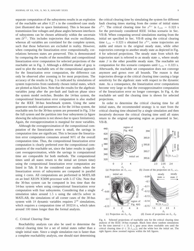
Reachability analysis can also be used to determine thecritical clearing time for a set of initial states rather than asingle initial state. Since a single simulation run is faster thana complete reachability analysis, one should start determining

the critical clearing time by simulating the system for differentfault clearing times starting from the center of initial statesx0,c. The critical clearing time forx0,c is tcrit = 0.323 sfor the previously considered IEEE 14-bus scenario in Sec.VII-B. When computing several simulations starting from theinitial set specified in Sec. VII-B using the critical clearingtime tcrit = 0.323 s obtained forx0,c, some trajectories arestable and return to the original steady state, while othertrajectories converge to another steady state as depicted in Fig.4 for selected projections. The steady state from which thetrajectories start is referred to as steady stateα, where steadystateβ is the other possible steady state. The reachable setcomputation for this scenario computes untiltcrit = 0.323 s.Afterwards, the reachable set computation does not convergeanymore and grows over all bounds. The reason is thattrajectories diverge at the critical clearing time causinga largesensitivity for the algebraic state with respect to the dynamicstate. As a consequence, the linearization error computationsbecome very large so that the overapproximative computationof the linearization error no longer converges. In Fig. 4, thereachable set until the clearing time is shown for selectedprojections.

In order to determine the critical clearing time for allinitial states, the recommended strategy is to start from thecritical clearing time obtained by a single simulation and theniteratively decrease the critical clearing time until all statesreturn to the original operating region as presented in Sec.VII-B.

0 2 4

320

340

360

380

400

420

440

δ1

ω1

initial set

region ofFig. 4(b)

(a) Projection onδ1, ω1.

2.3 2.35 2.4

393.6

393.7

393.8

393.9

394

δ1

ω1

R([0, tcrit])

steadystate

α

steadystate

β

(b) Zoom of the projection onδ1, ω1.

0 2 4 6−0.15

−0.1

−0.05

0

0.05

δ1

δ2

R([0,t c

rit])

initial set

region ofFig. 4(d)

(c) Projection onδ1, δ2.

1.5 2 2.5 3−0.15

−0.14

−0.13

−0.12

−0.11

−0.1

−0.09

δ1

δ2

R([0, tcrit])

steadystateα

steadystateβ

(d) Zoom of projection onδ1, δ2.

Fig. 4. Selected projections of reachable sets for the critical clearing timeanalysis of the IEEE 14-bus example. Black lines show randomsimulationsfor the time intervalt ∈ [0, 4] s, gray areas show reachable sets until thecritical clearing time (t ∈ [0, tcrit]), and the white box the initial set. Theright figures show zoomed regions within the left figures.

JOURNAL OF XX, VOL. X, NO. X, JANUARY XXXX 10

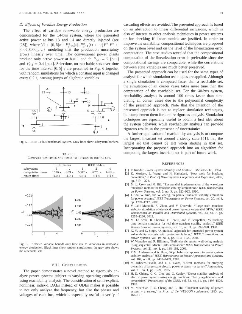
D. Effects of Variable Energy Production

The effect of variable renewable energy production aredemonstrated for the 14-bus system, where the generatedactive power at bus13 and 14 are directly injected (see[28]), where∀t ∈ [0, 5]s : P d

g,13(t), Pdg,14(t) ∈ { t

5P∗|P ∗ ∈

[0.04, 0.06]p.u.} modeling that the production uncertaintygrows linearly over time. The conventional power plantsproduce only active power at bus1 and 2: Pc,1 = 2 [p.u.]andPc,2 = 0.4 [p.u.]. Selections on reachable sets over timefor the time interval[0, 5] s are presented in Fig. 6 togetherwith random simulations for which a constant input is changedevery0.2 s, causing jumps of algebraic variables.

GG

GG

G

1

23

7 6

4

12 13 14

11 10

9 5

8

Fig. 5. IEEE 14-bus benchmark system. Gray lines show subsystem borders.

TABLE IICOMPUTATION TIMES AND TIMES TO RETURN TO INITIAL SET.

IEEE 14-bus IEEE 30-bussubsystems 1 2 1 2 4computation times 1536 s 853 s 5002 s 2025 s 1428 sreturn times 4.0 s 4.0 s 4.4 s 4.4 s 4.4 s

0 2 4

−0.24

−0.23

−0.22

−0.21

t

δ4

0 2 4

1.088

1.089

1.09

1.091

1.092

t

E4

Fig. 6. Selected variable bounds over time due to variationsin renewableenergy production. Black lines show random simulations, the gray area showsthe reachable sets.

VIII. C ONCLUSIONS

The paper demonstrates a novel method to rigorously an-alyze power systems subject to varying operating conditionsusing reachability analysis. The consideration of semi-explicit,nonlinear, index-1 DAEs instead of ODEs makes it possibleto not only analyze the frequency, but also the phases andvoltages of each bus, which is especially useful to verify if

cascading effects are avoided. The presented approach is basedon an abstraction to linear differential inclusions, whichisalso of interest to other analysis techniques in power systemsor for checking if linear models are justified. In order toimprove the scalability, compositional techniques are proposedon the system level and on the level of the linearization errorcomputation. The case studies revealed that the compositionalcomputation of the linearization error is preferable sincethecomputational savings are comparable, while the correlationsbetween state variables are much better preserved.

The presented approach can be used for the same types ofanalysis for which simulation techniques are applied. Althougha single simulation is computed faster than a reachable set,the simulation of all corner cases takes more time than thecomputation of the reachable set. For the30-bus system,reachability analysis is around100 times faster than sim-ulating all corner cases due to the polynomial complexityof the presented approach. Note that the intention of thepresented approach is not to replace simulation techniques,but complement them for a more rigorous analysis. Simulationtechniques are especially useful to obtain a first idea aboutthe system behavior, while reachability analysis can providerigorous results in the presence of uncertainties.

A further application of reachability analysis is to computethe largest invariant set around a steady state [51], i.e., thelargest set that cannot be left when starting in that set.Incorporating the proposed approach into an algorithm forcomputing the largest invariant set is part of future work.

REFERENCES

[1] P. Kundur,Power System Stability and Control. McGraw-Hill, 1994.[2] K. Morison, L. Wang, and H. Hamadani, “New tools for blackout

prevention,” inProc. of Power Systems Conference and Exposition, 2006,pp. 319 – 324.

[3] M. L. Crow and M. Ilic, “The parallel implementation of the waveformrelaxation method for transient stability simulations,”IEEE Transactionson Power Systems, vol. 5, no. 3, pp. 922–932, 1990.

[4] J. Shu, W. Xue, and W. Zheng, “A parallel transient stability simulationfor power systems,”IEEE Transactions on Power Systems, vol. 20, no. 4,pp. 1709–1717, 2005.

[5] V. Jalili-Marandi, Z. Zhou, and V. Dinavahi, “Large-scale transientstability simulation of electrical power systems on parallel GPUs,”IEEETransactions on Parallel and Distributed Systems, vol. 23, no. 7, pp.1255–1266, 2012.

[6] M. La Scala, R. Sbrizzai, F. Torelli, and P. Scarpellini,“A trackingtime domain simulator for real-time transient stability analysis,” IEEETransactions on Power Systems, vol. 13, no. 3, pp. 992–998, 1998.

[7] X. Yu and C. Singh, “A practical approach for integrated power systemvulnerability analysis with protection failures,”IEEE Transactions onPower Systems, vol. 19, no. 4, pp. 1811–1820, 2004.

[8] W. Wangdee and R. Billinton, “Bulk electric system well-being analysisusing sequential Monte Carlo simulation,”IEEE Transactions on PowerSystems, vol. 21, no. 1, pp. 188–193, 2006.

[9] P. M. Anderson and A. Bose, “A probabilistic approach to power systemstability analysis,”IEEE Transactions on Power Apparatus and Systems,vol. 102, no. 8, pp. 2430–2439, 1983.

[10] M. Ribbens-Pavella and F. J. Evans, “Direct methods forstudyingdynamics of large-scale electric power systems – a survey,”Automatica,vol. 21, no. 1, pp. 1–21, 1985.

[11] H.-D. Chiang, C.-C. Chu, and G. Cauley, “Direct stability analysis ofelectric power systems using energy functions: Theory, applications, andperspective,”Proceedings of the IEEE, vol. 83, no. 11, pp. 1497–1529,1995.

[12] M. Moechtar, T. C. Cheng, and L. Hu, “Transient stability of powersystem – a survey,” inProc. of the WESCON conference, 1995, pp.166–171.

JOURNAL OF XX, VOL. X, NO. X, JANUARY XXXX 11

[13] L. F. C. Alberto, F. H. J. R. Silva, and N. G. Bretas, “Direct methodsfor transient stability analysis in power systems: State ofart and futureperspectives,” inProc. of the IEEE Porto Power Tech Conference, 2001.

[14] U. Gabrijel and R. Mihalic, “Direct methods for transient stabilityassessment in power systems comprising controllable series devices,”IEEE Transactions on Power Systems, vol. 17, no. 4, pp. 1116–1122,2002.

[15] L. F. C. Alberto and H.-D. Chiang, “An uniform approach for directtransient stability analysis of electric power systems,” in Proc. of theIEEE Power & Energy Society General Meeting, 2009, pp. 1–7.

[16] A. R. Bergen, D. J. Hill, and C. L. de Marcot, “Lyapunov functionfor multimachine power systems with generator flux decay andvoltagedependent loads,”International Journal of Electrical Power & EnergySystems, vol. 8, no. 1, pp. 2–10, 1986.

[17] P. W. Sauer, A. K. Behera, M. A. Pai, J. R. Winkelman, and J. H. Chow,“Trajectory approximation for direct energy methods that use sustainedfaults with detailed power system models,”IEEE Transactions on PowerSystems, vol. 4, no. 2, pp. 499–506, 1989.

[18] I. A. Hiskens and D. J. Hill, “Energy functions, transient stabilityand voltage behavior in power systems with nonlinear loads,” IEEETransactions on Power Systems, vol. 4, no. 4, pp. 1525–1533, 1989.

[19] Y. Zou, M.-H. Yin, and H.-D. Chiang, “Theoretical foundation ofthe controlling UEP method for direct transient-stabilityanalysis ofnetwork-preserving power system models,”IEEE Transactions on Cir-cuits and Systems I: Fundamental Theory and Applications, vol. 50,no. 10, pp. 1324–1336, 2003.

[20] A. Platzer and E. M. Clarke, “The image computation problem in hybridsystems model checking,” inHybrid Systems: Computation and Control,ser. LNCS 4416. Springer, 2007, p. 473486.

[21] E. Asarin, T. Dang, G. Frehse, A. Girard, C. Le Guernic, and O. Maler,“Recent progress in continuous and hybrid reachability analysis,” inProc. of the 2006 IEEE Conference on Computer Aided Control SystemsDesign, 2006, pp. 1582–1587.

[22] C. Le Guernic, “Reachability analysis of hybrid systems with linearcontinuous dynamics,” Ph.D. dissertation, Univerite Joseph Fourier,2009.

[23] M. Althoff, “Reachability analysis and its applicationto the safety assessment of autonomous cars,” Disserta-tion, Technische Universitat Munchen, 2010, http://nbn-resolving.de/urn/resolver.pl?urn:nbn:de:bvb:91-diss-20100715-963752-1-4.

[24] S. Kaynama, “Scalable techniques for the computation of viable andreachable sets,” Ph.D. dissertation, The University of British Columbia,2012.

[25] L. Jin, H. Liu, R. Kumar, J. D. McCalley, N. Elia, and V. Aj-jarapu, “Power system transient stability design using reachability basedstability-region computation,” inProc. of the 37th Annual North Amer-ican Power Symposium, 2005, pp. 338–343.

[26] L. Jin, R. Kumar, and N. Elia, “Reachability analysis based transientstability design in power systems,”Electrical Power and Energy Systems,vol. 32, pp. 782–787, 2010.

[27] Y. Susuki, T. Sakiyama, T. Ochi, T. Uemura, and T. Hikihara, “Verifyingfault release control of power system via hybrid system reachability,” inProc. of the 40th North American Power Symposium, 2008.

[28] Y. C. Chen and A. D. Domınguez-Garcıa, “Assessing theimpact of windvariability on power system small-signal reachability,” in Proc. of theInternational Conference on System Sciences, 2011, pp. 1–8.

[29] ——, “A method to study the effect of renewable resource variability onpower system dynamics,”IEEE Transactions on Power Systems, vol. 27,no. 4, pp. 1978–1989, 2012.

[30] H. N. Villegas Pico, D. C. Aliprantis, and E. C. Hoff, “Reachabilityanalysis of power system frequency dynamics with new high-capacityHVAC and HVDC transmission lines,” inProc. of the IREP Bulk PowerSystem Dynamics and Control Symposium, 2013.

[31] M. Althoff, M. Cvetkovic, and M. Ilic, “Transient stability analysis byreachable set computation,” inProc. of the IEEE PES Conference onInnovative Smart Grid Technologies Europe, 2012.

[32] J. Machowski, J. Bialek, and J. Bumby,Power System Dynamics:Stability and Control. Wiley, 2008.

[33] M. Althoff, O. Stursberg, and M. Buss, “Reachability analysis of nonlin-ear systems with uncertain parameters using conservative linearization,”in Proc. of the 47th IEEE Conference on Decision and Control, 2008,pp. 4042–4048.

[34] K. Makino and M. Berz, “Rigorous integration of flows andODEs usingTaylor models,” inProc. of Symbolic-Numeric Computation, 2009, pp.79–84.

[35] G. Frehse, C. L. Guernic, A. Donze, S. Cotton, R. Ray, O.Lebeltel,R. Ripado, A. Girard, T. Dang, and O. Maler, “SpaceEx: Scalableverification of hybrid systems,” inProc. of the 23rd InternationalConference on Computer Aided Verification, ser. LNCS 6806. Springer,2011, pp. 379–395.

[36] M. Althoff, C. Le Guernic, and B. H. Krogh, “Reachable set compu-tation for uncertain time-varying linear systems,” inHybrid Systems:Computation and Control, 2011, pp. 93–102.

[37] M. Berz and G. Hoffstatter, “Computation and application of Taylorpolynomials with interval remainder bounds,”Reliable Computing,vol. 4, pp. 83–97, 1998.

[38] S. B. Yusof, G. J. Rogers, and R. T. H. Alden, “Slow coherency basednetwork partitioning including load buses,”IEEE Transactions on PowerSystems, vol. 8, no. 3, pp. 1375–1382, 1993.

[39] E. De Tuglie, S. M. Iannone, and F. Torelli, “A coherencyrecognitionbased on structural decomposition procedure,”IEEE Transactions onPower Systems, vol. 23, no. 2, pp. 555–563, 2008.

[40] C. S. Chang, L. R. Lu, and F. S. Wen, “Power system networkparti-tioning using tabu search,”Electric Power Systems Research, vol. 49,no. 1, pp. 55–61, 1999.

[41] A. Chutinan and B. H. Krogh, “Computational techniquesfor hybridsystem verification,”IEEE Transactions on Automatic Control, vol. 48,no. 1, pp. 64–75, 2003.

[42] A. Girard, C. Le Guernic, and O. Maler, “Efficient computation ofreachable sets of linear time-invariant systems with inputs,” in HybridSystems: Computation and Control, ser. LNCS 3927pl. Springer, 2006,pp. 257–271.

[43] A. B. Kurzhanski and P. Varaiya, “Ellipsoidal techniques for reachabilityanalysis,” in Hybrid Systems: Computation and Control, ser. LNCS1790. Springer, 2000, pp. 202–214.

[44] A. Girard and C. Le Guernic, “Efficient reachability analysis for linearsystems using support functions,” inProc. of the 17th IFAC WorldCongress, 2008, pp. 8966–8971.

[45] O. Stursberg and B. H. Krogh, “Efficient representationand computationof reachable sets for hybrid systems,” inHybrid Systems: Computationand Control, ser. LNCS 2623. Springer, 2003, pp. 482–497.

[46] A. Girard, “Reachability of uncertain linear systems using zonotopes,” inHybrid Systems: Computation and Control, ser. LNCS 3414. Springer,2005, pp. 291–305.

[47] W. Kuhn, “Rigorously computed orbits of dynamical systems withoutthe wrapping effect,”Computing, vol. 61, pp. 47–67, 1998.

[48] M. Althoff and B. H. Krogh, “Avoiding geometric intersection opera-tions in reachability analysis of hybrid systems,” inHybrid Systems:Computation and Control, 2012, pp. 45–54.

[49] University of Washington, “Power systems test case archive,” http://www.ee.washington.edu/research/pstca/, University of Washington.

[50] P. Schavemaker and L. van der Sluis,Electrical Power System Essentials.Wiley, 2008.

[51] S. V. Rakovic, P. Grieder, M. Kvasnica, D. Q. Mayne, andM. Morari,“Computation of invariant sets for piecewise affine discrete time systemssubject to bounded disturbances,” inProc. of the 43rd IEEE Conferenceon Decision and Control, 2004, pp. 1418–1423.

Matthias Althoff is assistant professor in computerscience at Technische Universitat Munchen, Ger-many. He received the diploma engineering degreein Mechanical Engineering in 2005, and the Ph.D.degree in Electrical Engineering in 2010, both fromTechnische Universitat Munchen, Germany. From2010 to 2012 he was a postdoctoral researcher atCarnegie Mellon University, Pittsburgh, USA, andfrom 2012 to 2013 an assistant professor at Tech-nische Universitat Ilmenau, Germany. His researchinterests include formal verification of continuous

and hybrid systems, reachability analysis, planning algorithms, nonlinearcontrol, automated vehicles, and power systems.