jss mahavidyapeetha jss science & technology … · department of mechanical engineering design...

Department of Mechanical Engineering Design Lab Manual

Sri Jayachamarajendra College of Engineering, Mysuru-06

JSS MAHAVIDYAPEETHA

JSS SCIENCE & TECHNOLOGY UNIVERSITY

(JSSS&TU) FORMERLY SRI JAYACHAMARAJENDRA COLLEGE OF ENGINEERING

MYSURU-570006

DEPARTMENT OF MECHANICAL ENGINEERING

Design Laboratory Manual VI Semester B.E. Mechanical Engineering

USN :_______________________________________

Name:_______________________________________

Roll No: __________ Sem __________ Sec ________

Course Name ________________________________

Course Code _______________________________



DEPARTMENT OF MECHANICAL ENGINEERING

VISION OF THE DEPARTMENT

Department of mechanical engineering is committed to prepare graduates, post graduates and

research scholars by providing them the best outcome based teaching-learning experience and

scholarship enriched with professional ethics.

MISSION OF THE DEPARTMENT

M-1: Prepare globally acceptable graduates, post graduates and research scholars for their

lifelong learning in Mechanical Engineering, Maintenance Engineering and Engineering

Management.

M-2: Develop futuristic perspective in Research towards Science, Mechanical Engineering

Maintenance Engineering and Engineering Management.

M-3: Establish collaborations with Industrial and Research organizations to form strategic and

meaningful partnerships.

PROGRAM SPECIFIC OUTCOMES (PSOs)

PSO1 Apply modern tools and skills in design and manufacturing to solve real world

problems.

PSO2 Apply managerial concepts and principles of management and drive global economic

growth.

PSO3 Apply thermal, fluid and materials fundamental knowledge and solve problem

concerning environmental issues.

PROGRAM EDUCATIONAL OBJECTIVES (PEOS)

PEO1: To apply industrial manufacturing design system tools and necessary skills in the field

of mechanical engineering in solving problems of the society.

PEO2: To apply principles of management and managerial concepts to enhance global

economic growth.

PEO3: To apply thermal, fluid and materials engineering concepts in solving problems

concerning environmental pollution and fossil fuel depletion and work towards

alternatives.



PROGRAM OUTCOMES (POS)

PO1 Engineering knowledge: Apply the knowledge of mathematics, science, engineering

fundamentals, and an engineering specialization to the solution of complex engineering

problems.

PO2 Problem analysis: Identify, formulate, review research literature, and analyze complex

engineering problems reaching substantiated conclusions using first principles of

mathematics, natural sciences, and engineering sciences.

PO3 Design/development of solutions: Design solutions for complex engineering problems and

design system components or processes that meet the specified needs with appropriate

consideration for the public health and safety, and the cultural, societal, and environmental

considerations.

PO4 Conduct investigations of complex problems: Use research-based knowledge and research

methods including design of experiments, analysis and interpretation of data, and synthesis

of the information to provide valid conclusions.

PO5 Modern tool usage: Create, select, and apply appropriate techniques, resources, and modern

engineering and IT tools including prediction and modeling to complex engineering activities

with an understanding of the limitations.

PO6 The engineer and society: Apply reasoning informed by the contextual knowledge to assess

societal, health, safety, legal and cultural issues and the consequent responsibilities relevant

to the professional engineering practice.

PO7 Environment and sustainability: Understand the impact of the professional engineering

solutions in societal and environmental contexts, and demonstrate the knowledge of, and

need for sustainable development.

PO8 Ethics: Apply ethical principles and commit to professional ethics and responsibilities and

norms of the engineering practice.

PO9 Individual and team work: Function effectively as an individual, and as a member or leader

in diverse teams, and in multidisciplinary settings.

PO10 Communication: Communicate effectively on complex engineering activities with the

engineering community and with society at large, such as, being able to comprehend and

write effective reports and design documentation, make effective presentations, and give and

receive clear instructions.

PO11 Project management and finance: Demonstrate knowledge and understanding of the

engineering and management principles and apply these to one‟s own work, as a member and

leader in a team, to manage projects and in multidisciplinary environments.

PO12 Life-long learning: Recognize the need for, and have the preparation and ability to engage in

independent and life-long learning in the broadest context of technological change.



DESIGN LABORATORY

Subject Code : ME67L No. of Credits : 0-0-1.5

No. of Contact Hours / Week : 03

CIE Marks

: 50 Total No. of Contact Hours : 39

COURSE OBJECTIVES:

1. To demonstrate the concepts discussed in Design of Machine Elements, Mechanical Vibrations &

Dynamics of Machines courses.

2. To visualize and understand the development of stresses in structural members and experimental

determination of stresses in members utilizing the optical method of reflected photo-elasticity.

COURSE CONTENT

Part-A

1. Determination of natural frequency of a spring mass system.

2. Determination of natural frequency logarithmic decrement, damping ratio and damping Co-efficient in a single

degree of freedom vibrating systems (longitudinal and torsional)

3. Determination of critical speed of rotating shaft.

4. Balancing of rotating masses.

Part-B

5. Determination of fringe constant of Photo-elastic material using Circular disk subjected diametric

compression, Pure bending specimen (four point bending)

6. Determination of equilibrium speed, sensitiveness, power and effort of Porter/Hartnell Governor.

7. Determination of pressure distribution in Journal bearing

8. Experiments on Gyroscope (Demonstration only)

REFERENCE BOOKS:

1. “Shigley‟s Mechanical Engineering Design”, Richards G. Budynas and J. Keith Nisbett, McGraw-Hill

Education, 10th

Edition, 2015.

2. “Design of Machine Elements”, V.B. Bhandari, TMH publishing company Ltd. New Delhi, 2nd

Edition 2007.

3. “Theory of Machines”, Sadhu Singh, Pearson Education, 2nd

Edition, 2007.

4. “Mechanical Vibrations”, G.K. Grover, Nem Chandand Bros, 6th

Edition, 1996.

COURSE OUTCOMES:

Upon completion of this course, students should be able to:

CO1 To practically relate to concepts discussed in Design of Machine Elements, Mechanical Vibrations &

Dynamics of Machines courses.

CO2 To measure strain in various machine elements using strain gauges and determine strain induced in a

structural member using the principle of photo-elasticity.



CONTENTS Experiment No. Name of the Experiment Page No.

1. Spring Mass System

1-6

2. Torsional Viscous Damper System

7-11

3. Spring Mass Damper System

12-13

4. Critical Speed Of Shaft Or Whirling Of Shaft

14-21

5. Spring Controlled Governor

22-25

6. Balancing Of Rotating Masses

26-31

7. Journal Bearing Test Rig

32-37

8. Photo Elastic Test Bench

38-42

9. Gyroscope

43-47



Experiment #1

SPRING MASS SYSTEM

Aim:

1. To determine the spring constant of the given spring.

2. To determine the natural frequency and compare the same with the

Theoretical frequency of:

a. Springs in parallel

b. Spring Mass System

c. Spring in Series

Apparatus: Springs, Rigid Frame, Scale, Stop Watch, Pan and Weights.

Theory: Students should write about static equilibrium position, natural frequency,

derive expression for natural frequency for free vibrating body, derive expression

for springs in series and parallel.



Equation of Motion: Natural Frequency

Above figure shows a simple undamped spring-mass system, which is assumed to

move only along the vertical direction. It has one degree of freedom (DOF), because

its motion is described by a single coordinate x.

When placed into motion, oscillation will take place at the natural frequency 𝑓𝑛 which

is a property of the system. We now examine some of the basic concepts associated

with the free vibration of systems with one degree of freedom.

Newton's second law is the first basis for examining the motion of the system. As

shown in Figure. The deformation of the spring in the static equilibrium position is ∆,

and the spring force 𝑘∆ is equal to the gravitational force w acting on mass „m‟

k∆= 𝑤 = 𝑚𝑔

By measuring the displacement x from the static equilibrium position, the forces

acting on „m’ are 𝑘 ∆ + 𝑥 and „𝑤’. With „𝑥’ chosen to be positive in the downward

direction, all quantities - force, velocity, and acceleration are also positive in the

downward direction.

We now apply Newton's second law of motion to the mass m:

𝑚𝑥 𝐹 = 𝑤 − 𝑘(∆ + 𝑥)

and because 𝑘∆= 𝑤, we obtain :

𝑚𝑥 = −𝑘𝑥 where 𝜔𝑛 2 =

𝜆

𝑚

𝑥 + 𝜔𝑛2

and we conclude that the motion is harmonic. A homogeneous second order linear

differential equation has the following general solution:

𝒙 = 𝑨𝐬𝐢𝐧𝝎𝒏 𝒕 + 𝑩𝐜𝐨𝐬𝝎𝒏𝒕

where „A‟ and „B’ are the two necessary constants. These constants are evaluated

from initial conditions 𝑥 0 and𝑥 0 ,

𝒙 = 𝒙 𝟎

𝝎𝒏𝐬𝐢𝐧𝝎𝒏𝒕 + 𝒙 𝟎 𝐜𝐨𝐬𝝎𝒏 𝒕



The natural period of the oscillation is established from, 𝜔𝑛𝑡 = 2𝜋 or

𝒕 = 𝟐𝝅 𝒎

𝒌

and the natural frequency is

𝒇𝒏 = 𝟏

𝒕=

𝟏

𝟐𝝅 𝒌

𝒎

These quantities can be expressed in terms of the static deflection „∆‟ by observing ,

𝑘∆ = 𝑚𝑔. Thus natural frequency can be expressed in terms of the static deflection

„∆‟ as

𝒇𝒏 = 𝟏

𝟐𝝅 𝒈

∆

Note that 𝜏, 𝑓𝑛 and 𝜔𝑛 , depend only on the mass and stiffness of the system, which

are properties of the system.

Spring in Series 𝟏

𝒌𝒆𝒒=

𝟏

𝒌𝟏+

𝟏

𝒌𝟐

Springs in parallel 𝒌𝒆𝒒 = 𝒌𝟏 + 𝒌𝟐



Procedure:

1. To determine the spring stiffness:

a. Take the initial length of the spring.

b. Fix the spring to the frame and the pan to the other end of the spring.

c. The spring stretches due to pan weight. Take the final length.

d. Add weights to the pan and take the final length of the spring.

corresponding to the weights added and tabulate the results.

e. The above procedure is repeated for other springs.

Sl

NO.

Weight in

Kgs

Initial

Length in

mm

Final

Length in

mm

Static

deflection in

mm

Spring

stiffness in

N/mm

Average

spring

stiffness in

N /mm

1.

2.

3.

𝑘∆ = 𝑤 = 𝑚𝑔

𝒌 = 𝒎𝒈

∆ N/ mm

2. To determine the natural frequency of spring mass system and

compare it with the theoretical frequency:

Procedure:

a. Fix the spring to the rigid frame and attach pan to it.

b. Stretch the pan down and release it. The system oscillates. Note down the time

taken for 10 oscillations.

c. Repeat the above step with different weights on the pan and tabulate the

results.



Sl

No.

Weight in

Kgs

Times taken

for 10

oscillations in

sec

Frequency =

𝒏/𝒕 CPS or HZ

Theoretical

frequency in

CPS or HZ

Error= theoretical

frequency- actual

frequency

K = spring stiffness used in the experiment in N /mm

𝒇𝒏 = 𝟏

𝑻=

𝟏

𝟐𝝅

𝒌

𝒎 in cps or Hz

3. To determine the natural frequency of spring mass system for springs in

series and compare it with the theoretical frequency:

Procedure:

a. Fix the spring to the rigid frame. Attach the second spring to the first spring

and attach pan to it.

b. Stretch the pan down and release it. The system oscillates. Note down the

time taken for 10 oscillations.


results

Where 𝑘𝑒 is the equivalent spring stiffness in N /mm

𝒇𝒏 = 𝟏

𝑻=

𝟏

𝟐𝝅

𝒌𝒆

𝒎 in CP or Hz

Sl

No.

Weight in

Kgs

Times taken for

10 oscillations

in sec

Frequency =

𝒏/𝒕 CPS or HZ

Theoretical

frequency in

CPS or HZ

Error =

theoretical

frequency-

actual

frequency



4. To determine the natural frequency of spring mass system for

springs in Parallel and compare it with the theoretical frequency:

Procedure:

a. Fix the spring to the rigid frame. Attach the second spring parallel to the first

spring. Insert a rod and attach pan at the center of the rod.

b. Stretch the pan down and release it. The system oscillates. Note down the

time taken for 10 oscillations.


results.

Sl

No.

Weight in

Kgs

Times taken for

10 oscillations

in sec

Frequency =

𝒏/𝒕 CPS or HZ

Theoretical

frequency in

CPS or HZ

Error=Theoretical

frequency- actual

frequency

Specimen Calculation:

Natural frequency, (theoretical) 𝜔𝑛 = 𝑘𝑒

𝑚 rad /sec

𝒇𝒏 = 𝟏

𝑻=

𝟏

𝟐𝝅 𝒌𝒆

𝒎

Inference of the Results:



Experiment #2

TORSIONAL VISCOUS DAMPER SYSTEM

Aim: To determine the natural frequency of the damped system, logarithmic

decrement, damping ratio and damping factor for different depth of

immersion of the disc in a viscous medium (OIL).

Apparatus: Torsional system with a rod and disc attached to the rigid frame, an

oil bath and weights to increase the depth of immersion.

Theory: Students have to write about damping and its effect on the system,

different types of damping, derive expression for logarithmic decrement

and establish a relation between logarithmic decrement and damping

ratio.

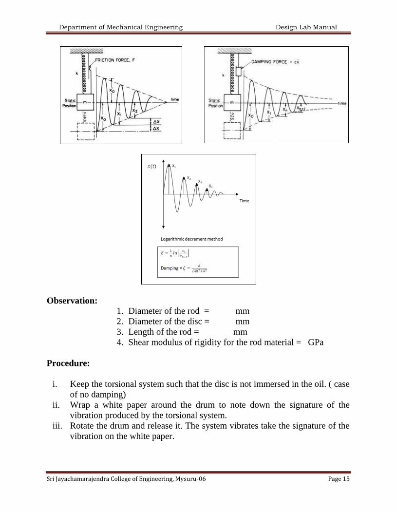
Viscous Damping

It is encountered by bodies moving at moderate speed through liquid. This type of

damping leads to a resisting force proportional to the velocity. The damping force

𝐹𝑑 ∝ 𝑑𝑥

𝑑𝑡

𝐹𝑑 = 𝑐𝑥

„c‟ is the constant of proportionality and is called viscous damping Co-efficient.

With the dimension of N-S/m



Coulomb Damping

This type of damping arises from sliding of dry surfaces. The friction force is

nearly constant and depends upon the nature of sliding surface and normal pressure

between them as expressed by the equation of kinetic friction

𝐹 = 𝜇𝑁

Where 𝜇 = co-efficient of friction

N = normal force

Solid or structural Damping

This is due to internal friction within the material itself. Experiment indicates that

the solid damping differs from viscous damping in that it is independent of

frequency and proportional to maximum stress of vibration cycle.

Slip or Intrefacial damping

Energy of vibration is dissipated by microscopic slip on the interfaces of machine

parts in contact under fluctuating loads. Microscopic slip also occurs on the

interface of the machine elements having various types of joints. This type is

essentially of a linear type.



Observation:

1. Diameter of the rod = mm

2. Diameter of the disc = mm

3. Length of the rod = mm

4. Shear modulus of rigidity for the rod material = GPa

Procedure:

i. Keep the torsional system such that the disc is not immersed in the oil. ( case

of no damping)

ii. Wrap a white paper around the drum to note down the signature of the

vibration produced by the torsional system.

iii. Rotate the drum and release it. The system vibrates take the signature of the

vibration on the white paper.



iv. Raise the oil drum so as to dip the disc of the torsional system in the oil to

produce viscous damping. This is done by placing weights below the drum.

Twist the drum and take down the signature on the white paper.

v. Repeat the procedure for three depths of immersion and tabulate the results.

vi. Plot a graph of depth of immersion V/S damping coefficient.

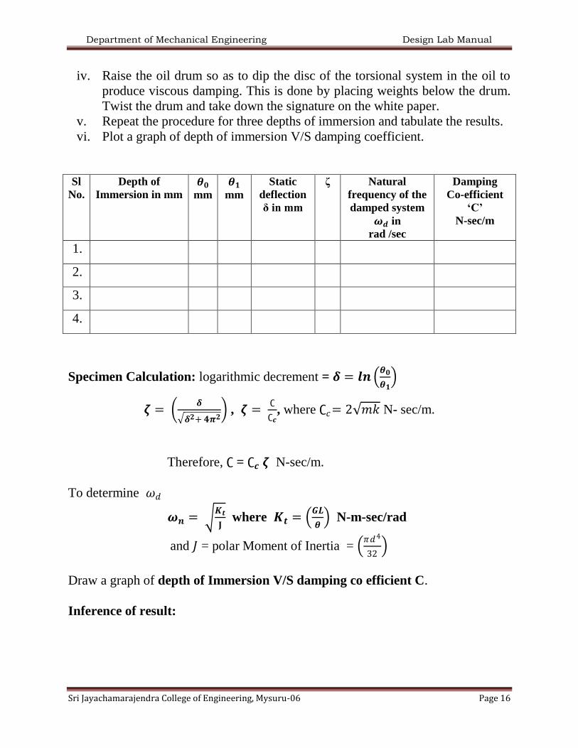
Sl

No.

Depth of

Immersion in mm

𝜽𝟎

mm

𝜽𝟏

mm

Static

deflection

δ in mm

ζ Natural

frequency of the

damped system

𝝎𝒅 in

rad /sec

Damping

Co-efficient

‘C’

N-sec/m

1.

2.

3.

4.

Specimen Calculation: logarithmic decrement = 𝜹 = 𝒍𝒏 𝜽𝟎

𝜽𝟏

𝜻 = 𝜹

𝜹𝟐+ 𝟒𝝅𝟐 , 𝜻 =

∁

∁𝒄, where ∁𝑐= 2 𝑚𝑘 N- sec/m.

Therefore, ∁ = ∁𝒄 𝜻 N-sec/m.

To determine 𝜔𝑑

𝝎𝒏 = 𝑲𝒕

𝐉 where 𝑲𝒕 =

𝑮𝑳

𝜽 N-m-sec/rad

and 𝐽 = polar Moment of Inertia = 𝜋𝑑4

32

Draw a graph of depth of Immersion V/S damping co efficient C.

Inference of result:



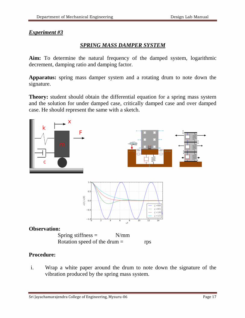
Experiment #3

SPRING MASS DAMPER SYSTEM

Aim: To determine the natural frequency of the damped system, logarithmic

decrement, damping ratio and damping factor.

Apparatus: spring mass damper system and a rotating drum to note down the

signature.

Theory: student should obtain the differential equation for a spring mass system

and the solution for under damped case, critically damped case and over damped

case. He should represent the same with a sketch.

Observation:

Spring stiffness = N/mm

Rotation speed of the drum = rps

Procedure:

i. Wrap a white paper around the drum to note down the signature of the

vibration produced by the spring mass system.



ii. Place a weight on the pan and release the system to vibrate. Take the

signature on the rotating drum.

iii. Repeat the procedure for three weights and tabulate the results.

iv. Plot a graph of depth of immersion V/S damping coefficient.

Sl

No.

Mass in

kg

Wave

length

λ in m

θ0

mm

θ1

mm

Static

deflection

δ in mm

𝜻 Natural

frequency

of the

damped

system 𝝎𝒅

in rad /sec

Damping

Co-efficient ‘C’

N-sec/m

1.

2.

3.

4.

Specimen Calculation: 𝒇𝒅 = 𝑽

𝝀 cps or Hz.

where 𝑉 = velocity in m/sec and λ is in m

logarithmic decrement = 𝜹 = 𝒍𝒏𝜽𝟎

𝜽𝟏

𝜁 = 𝛿

𝛿2+4𝜋2 , 𝜻 =

𝑪

𝑪𝒄 where 𝑪𝒄 = 𝟐 𝒎𝒌 N- sec/m

Therefore, 𝑪 = 𝑪𝒄 𝜻 N-sec/m.

Inference of result:



Experiment #4

CRITICAL SPEED OF SHAFT OR WHIRLING OF SHAFT

Aim: To determine the critical speed of the shaft.

Apparatus: Disc mounted at the center of a rotating shaft, the shaft is supported in

bearings, a motor is coupled to the shaft and the motor is connected to the variac

for speed adjustment. A stroboscope is provided to note down the speed of the

shaft.

Theory: students are expected to write about critical speed of shat or whirling of

shaft or whipping of shaft and it importance. The student should derive an

expression for critical speed of shat and discuss the four conditions in critical speed

of shaft.



𝚾

𝒆=

𝒎𝝎𝑴

𝒌𝑴− 𝝎𝟐

𝟐

+ 𝒄𝑴𝝎

𝟐

𝚾

𝒆

𝑴

𝒎=

𝝎𝝎𝒏

𝟏 − 𝝎𝝎𝒏

𝟐

𝟐

+ 𝟐𝜻𝝎𝝎𝒏

𝟐

Since, 𝒄

𝒎= 𝟐𝜻𝝎𝒏 and 𝝎𝒏 =

𝒌

𝒎

𝐭𝐚𝐧𝝓 = 𝟐𝜻 𝝎 𝝎𝒏

𝟏 − 𝝎𝝎𝒏

𝟐

𝒄𝝎

𝒌 −𝒎𝝎𝟐



Critical (Whirling) Speed of Shafts

Introduction

For a rotating shaft there is a speed at which, for any small initial deflection, the

centripetal force is equal to the elastic restoring force. At this point the deflection

increases greatly and the shaft is said to “whirl”. Below and above this speed this

effect is very much reduced. This critical (whirling speed) is dependent on the

shaft dimensions, the shaft material and the shaft loads. The critical speed is the

same as the frequency of traverse vibrations.

The critical speed „𝑁𝑐 ′of a shaft is simply

𝑁𝑐 =

𝑘𝑚

2𝜋

Where m = the mass of the shaft assumed concentrated at single point.

„k‟ is the stiffness of the shaft to traverse vibrations

For a horizontal shaft this can be expressed as

𝑁𝑐 =

𝑔

𝑦

2𝜋

Where y = the static deflection at the location of the concentrated mass.

Symbols m = Mass (kg) E =Young‟s Modulus (N/m

2)

Nc = critical speed (rev/s ) I = Second Moment of Area (m4)

g = acceleration due to gravity (m.s-2

) y = deflection from δ with shaft

rotation

O = centroid location δ = static deflection (m)

G = Centre of Gravity location ω = angular velocity of shaft (rads/s)

L = Length of shaft



Theory

Consider a rotating horizontal shaft with a central mass (m) which has a centre of

gravity (G) slightly away from the geometric centroid (O)

The centrifugal force on the shaft = m ω 2(y + e) and the inward pull exerted by the

shaft y =48𝐸𝐼

𝐿3 The more general formulae for the restoring traverse force of the

beam is y (K EI / L 3) where K = a constant depending on the position of the mass

and the end fixing conditions.

Equating these forces…

When the denominator = 0, that is [ KEI / m ω 2 L

3 ] = 1 , the deflection becomes

infinite and whirling takes place.

The whirling or critical speed is therefore.

For a simply supported beam with a central mass K = 48. See examples below

Substituting ω c 2 for KEI /mL

3 in the above equation for y results in the following

equation which relates the angular velocity with the deflection.



This is plotted below.

This curve shows the deflection of the shaft (from the static deflection position) at

any speed ω in terms of the critical speed.

When ω < ωc the deflection y and e have the same sign that is G lies outside of

O. When ω > ωc then y and e are of opposite signs and G lies between the centre

of the rotating shaft and the static deflection curve. At high speed G will move

such that it tends to coincide with the static deflection curve.

Cantilever rotating mass

Mass of shaft neglected

Central rotating mass- Long Bearings




Central rotating mass – Short Bearings


Non-Central rotating mass – Short Bearings


Cantilevered Shaft

m = mass /unit length

Shaft Between short bearings




Shaft Between long bearings


Combined loading

This is known as Dunkerley‟s method an is based on the theory of superposition….



Procedure:

i. Measure the distance between the supports and fix the disc at the center of

the shaft.

ii. Slowly rotate the variac so as to rotate the shaft.

iii. Keep on observing for the vibration on the shaft.

iv. When the shaft starts vibrating observe the amount of vibration in the shaft.

v. Note down the speed at which the shaft vibrates violently. This will be the

critical speed of the shaft.

vi. Repeat the procedure at least three times and note down the critical speed.

Tabulate the result and compare it with the theoretical critical speed.

Sl No. Critical speed in rpm ( actual) Critical speed

theoretical in rpm

Error

1.

2.

3.

Inference:



Experiment # 5

SPRING CONTROLLED GOVERNOR

Aim: To determine the equilibrium speed at different radius of rotation and to

draw the controlling force diagram.

Apparatus: Governor, Motor and Variance.

Theory:

The function of governor is, in all operating conditions, to adjust the fuel injection

pump and ensure the stable operation of diesel engine at regulated speed when the

load changes. The loads and speeds of cars, tractors and diesel engine are

constantly changing. Climbing automobiles and sailing ships are often influenced

by wind, water and other environmental factors, which leads to changes in engine

load. If the ship is in a rough sea, the storm may make the ship swing left and right,

after and forth, sometimes, even the propeller expose in the air and the load reduce

suddenly, then if the supplication of the fuel can‟t be reduced in time, the speed of

the engine will escalate suddenly, and lead to “runaway”. Conversely, a sudden

increase in engine load, particularly in the low-speed operation, if the oil

supplication cannot increase promptly, the engine may stops working. As the

engine load changes large and quickly, it is difficult for manual control of fuel

supplication, and even impossible. In order to adjust the fuel supplication to the

load changes automatically, and ensure stabled engine operation, governor is

equipped.

In addition, in the diesel generators, to ensure the stable voltage and constant speed

operation, diesel is also equipped with governors. In short, the functions of

governor can be summarized as follows:

To prevent speeding diesel (runaway) operation-control the maximum speed;

Ensure stable operation at low speed-control minimum stable speed; control the

engine run at regulated speed. With the load outside changes, automatically adjust

fuel supplication; ensure the engine always operates at regular speed stabile.

According to the different control mechanism, governor can be classified into:



Dead weight governor and Spring Controlled governor. Dead weight governors are

Porter and Proell Governor Hatnell Governor is a spring controlled governors.

Note: The student is expected to derive an express for spring controlled governor

used in the set up. The student should also write about sensitiveness, equilibrium

speed, isochronisms and stability and effort of a governor.



Total lift = (x1+x2) = (b θ1+ b θ2)

= b (θ1+ θ2)

= b ((𝑟−𝑟1)

𝑎+

(𝑟2−𝑟)

𝑎) =

𝑏

𝑎 (𝑟2 − 𝑟1)

s2-s1 = Total lift × s = 𝑏

𝑎 (𝑟2 − 𝑟1) s

∴ (Fc)2 -(Fc)1 = 𝑏

𝑎

2 (𝑟2−𝑟1)

2 s

or stiffness of spring 's' = 2 𝑎

𝑏

2 (Fc )2 −(Fc )1

(𝑟2−𝑟1)

Observations:

Mass of each ball = Kg

Height of the sleeve = mm

Radius of Rotation= mm

Procedure: Take the various dimension of the governor like radius of rotation,

height of the sleeve and ball weight.

1. Using the variance increase the speed of the governor. The fly balls fly out and the

sleeve is lifted. Not down the radius of rotation and the sleeve lift for that

particular speed of the governor.



2. Repeat the above step for different speeds and tabulate the results

Sl No. Speed in rpm Radius of

rotation in mm

Sleeve lift in

mm

Centrifugal Force

in N

1.

2.

3.

4.

Inference:



Experiment # 6

BALANCING OF ROTATING MASSES

Aim: To determine the balancing mass for the disturbing mass in the same plane

and balancing of disturbing masses in different planes.

Apparatus: Balancing mass set up, weights and variance.

Theory: Consider a shaft rotating with an angular velocity „ω‟. If a mass, m is

attached to that shaft, it exert a centrifugal force on the shaft which tends the shaft

to bend or to vibrate it. This is an undesirable phenomenon in the case of a rotating

shaft and in order to avoid these things, we are using the technique of Balancing of

Rotating Masses. By this process, another mass is attached to the opposite side of

the first mass so that the centrifugal force created by the second mass cancels out

that produced by the first mass. By this, the vibrations in the shaft can be avoided.

The process of selecting and using the second mass in such a manner that its effect

counter acts the effect of centrifugal force of the first mass is known as the

Balancing of Rotating Masses.

The balancing of rotating masses at various situations is described below:

1. Balancing of Single Rotating Mass by a single mass rotating in the same plane:

The figure shows the situation of balancing of a single rotating mass by a single

mass rotating in the same plane. According to the situation,

FC1 = FC2

http://www.spectrose.com/wp-content/uploads/2012/08/BM-1.jpg



→ m1r1(ω)2= m2r2(ω)

2

→ m1r1 = m2r2

2. Balancing of Single Rotating Mass by Two rotating masses in different planes:

The figure shows the situation of balancing of a single rotating mass by Two

rotating masses in different planes. According to the situation, two considerations

can be taken into account.

a) FC = FC1+FC2

→ mr(ω)2 = m1r1(ω)

2 + m2r2(ω)

2

→mr = m1r1 + m2r2

Taking Moment about P:

FC1*d = FC*d2

→m1r1d = mrd2

→m1r1 = mr(d2/d)

Taking Moment about Q:

FC2*d = FC*d1

→m2r2d = mrd1

→m2r2 = mr(d1/d)

http://www.spectrose.com/wp-content/uploads/2012/08/BM2-copy.jpg



b)

FC+FC2 = FC1

→mr+m2r2 = m1r1

Taking Moments about P:

→m1r1 = mr(d2/d)

Taking Moments about Q:

→ m2r2 = mr(d1/d)

There are many other situations where balancing of rotating masses should be

done. Examples are:

3. Several masses rotating in the same plane.

4. Several masses rotating in different planes.

These situations will be considered in the coming posts.



http://www.spectrose.com/wp-content/uploads/2012/08/BM3-copy.jpg



Static (Single Plane) Balance -

mbRbx = - S(miRix) from i = 1 to n

mbRby = - S(miRiy) from i = 1 to n

fb = arctan[(mbRby)/(mbRbx)]

mbRbx = [(mbRbx)2 + (mbRby)

2]

1/2

mb = balance mass

Rb = radial distance to CG of balance mass

mi = i th point mass

Ri = radial distance to CG of the i th point mass

fb = angle of rotation of balance mass CG with respect to the reference

axis.

x, y = subscripts that designate orthogonal components

Two balance masses are added (or subtracted), one each on planes A and B.

mBRBx = - S(miRixli) from i = 1 to n

mBRBy = - S(miRiyli) from i = 1 to n

mARAx = - S(miRix) - mBRBx from i = 1 to n

mARAy = - S(miRiy) - mBRBy from i = 1 to n

mA = balance mass in the A plane

mB = balance mass in the B plane

RA = radial distance to CG of balance mass

RB = radial distance to CG of balance mass

fA, fB, RA, RB are found using relationships in Static Balance above



Ignoring the weight of the tire and its reactions at 1 and 2,

F1x + F2x mARAxw2 + mBRBxw

2 = 0

F1y + F2y mARAyw2 + mBRByw

2 = 0

F1x l1 + F2x l2 + mBRBxw2

lB = 0

F1y l1 + F2y l2 + mBRByw2

lB = 0

mBRBx = (F1x l1 + F2x l2)/( lBw2)

mBRBy = (F1y l1 + F2y l2)/( lBw2)

mARAx = (F1x + F2x)/(w2) - mbRBx

mARAy = (F1y + F2y)/(w2) - mbRBy


Sri Jayachamarajendra College of Engineering, Mysuru-06 Page 3

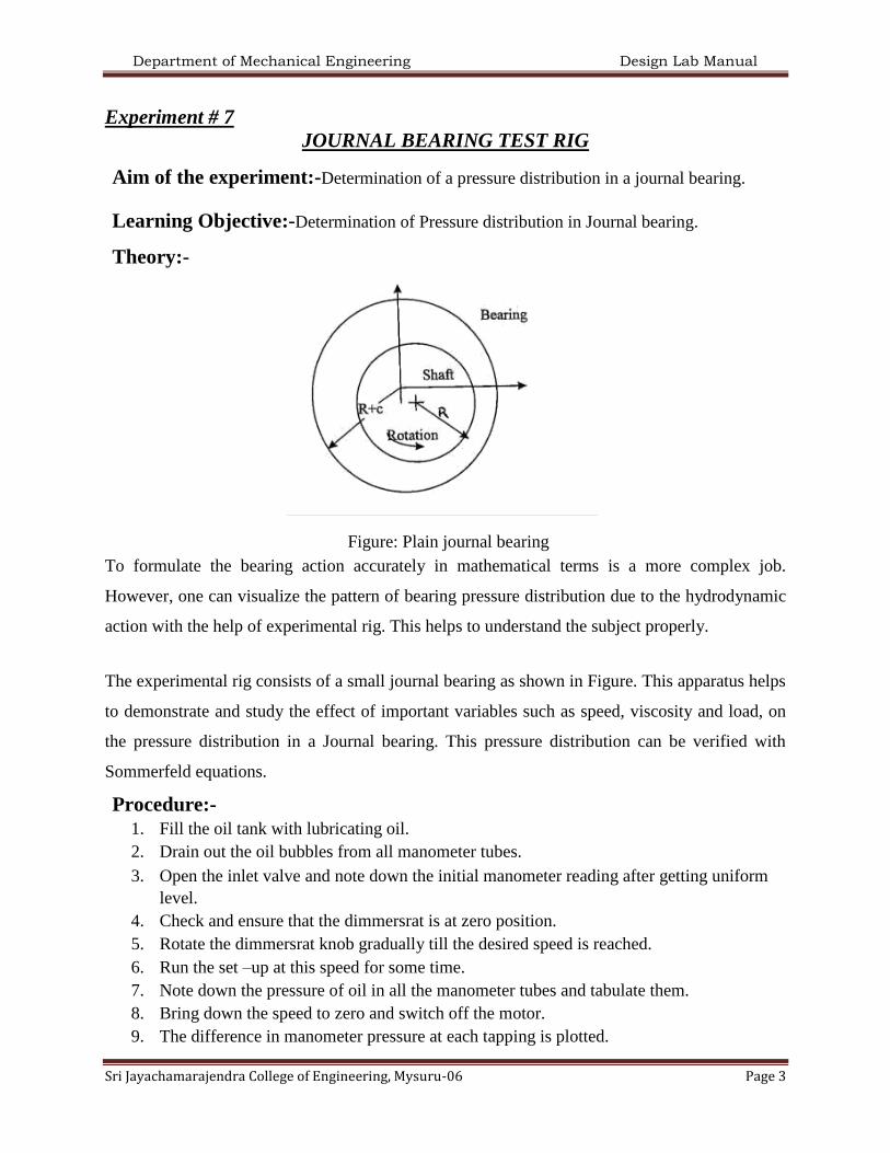
Experiment # 7

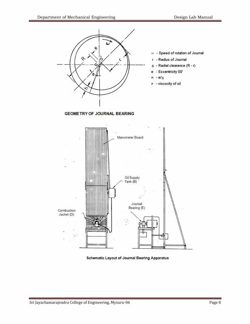
JOURNAL BEARING TEST RIG

Aim of the experiment:-Determination of a pressure distribution in a journal bearing.

Learning Objective:-Determination of Pressure distribution in Journal bearing.

Theory:-

Figure: Plain journal bearing

To formulate the bearing action accurately in mathematical terms is a more complex job.

However, one can visualize the pattern of bearing pressure distribution due to the hydrodynamic

action with the help of experimental rig. This helps to understand the subject properly.

The experimental rig consists of a small journal bearing as shown in Figure. This apparatus helps

to demonstrate and study the effect of important variables such as speed, viscosity and load, on

the pressure distribution in a Journal bearing. This pressure distribution can be verified with

Sommerfeld equations.

Procedure:-

1. Fill the oil tank with lubricating oil. 2. Drain out the oil bubbles from all manometer tubes. 3. Open the inlet valve and note down the initial manometer reading after getting uniform

level. 4. Check and ensure that the dimmersrat is at zero position. 5. Rotate the dimmersrat knob gradually till the desired speed is reached. 6. Run the set –up at this speed for some time. 7. Note down the pressure of oil in all the manometer tubes and tabulate them. 8. Bring down the speed to zero and switch off the motor. 9. The difference in manometer pressure at each tapping is plotted.



THEORY OF JOURNAL BEARINGS

The mathematical analysis of the behaviour of a journal in a bearing fails into two

distinct categories as given in the appendix to this Manual. They are:

1. Hydrodynamics of fluid flow between plates.

2. Journal bearing analysis where the motion of the journal in the oil film is considered.

According to equation the Sommerfield pressure function (when the velocity of the eccentricity

and the whirl speed of the journal are both zero is given by :

222

2ω

ocosθon(1

cosθonsinθinnx

)n(2δ

r6μPP

Where P is the pressure of the oil film at the point measured clockwise from the line of common

centers (oo‟) and P = Po at = 0 and = (refer to Fig. No. 2)

Note : Some books on lubication gives the sommerfield function with a negative sign for n.

This is true if it is measured from the point of minimum thickness of the oil films that is

)cos1(h n

Maximum pressure occurs at 22

3Cos

n

nm

Hence minimum pressure occurs at the point = -em. The total load (P) on the journal is given

by equation (acting perpendicular the line of centers oo‟)

222

3

1

1

n2

nx

δ

rμ12P

nx

L

Where L is width of the bearing and the total force along oo‟ is zero.

The total tractional couple „M‟ necessary to rotate the journal is given by

22

23

1)n(2

2n1x

δ

rμ4M

n

L

Note:

i) When comparing the above expressions for pressures, loads and so on, with experimental

data obtained from the small journal bearing rig, must be measured from the point where

the thickness of the oil films is maximum and in the anti clockwise direction.



ii) P-Po = 0 at = 0 and =

i.e. P = Po at 180° apart from zero.

That is on the pressure curve (head of oil/angular position) select two points of equal

pressure 180 apart. Of these two points take as Origin the point where the thickness of the oil

film is greater, and measure anti clockwise to plot the Summerfield pressure curve -after

determining graphically the values of 'n' from:

22

3

n

nmCos

and the value of „k‟ in

Where „K‟ has some units of dimensions as „P‟, „n‟ is non-dimensional.

Determine the pressure distribution in the oil film of the bearing for various speeds and

a) Plot the Cartesian and polar pressure curves for various speeds.

222

3

1

1

2

12

nx

n

nx

LwrP

And compare with load on the bearing. Determination of Tractional torque.

LOAD ON BEARING:

01. Total vertical load on bearing at N.R.P.M.

= Dry weight of bearing + weight added + weight of balancing load.

= 1.375 Kg. + 2 x 0.1150 Kg. + added weight Nil.

= 1.6775 Kg.

02. Referring to Fig. No.4, the mean positive pressure head of oil above supply head -

= (35.5 + 24 +12 + 8 +5 +2 +60 + 177 + 130)/10 = 45.5 cms.

Load carried by oil pressure on projected area of bearing –

= 45.5 x density of oil x (2R) L

= 45.5 x 0.8539 x 5.5 x 6.8

= 1.450 Kg.

Note: The underlined figures are recorded from graph and balanced are practical results.

03. Maximum theoretical load on Journal is „P‟.



2221

1

2

12

nn

nx

LrP

oilofdensityxn

LrxK

2

3

1

2

8539.08.01

8.62

5142.325.24

2x

xxxx

P = 3.724Kgs.

04. Tractional Torque = Balancing weight J x Length of arm of the weight L.

Table – 1

TYPICAL RESULTS w.r.t.

MANOMETER TUBES

Ps = Supply head =

Weight of bearing =

TABLE –2

PRESSURE HEAD OF OIL

FILM ABOVE HEAD

(P-Ps) cm. : _________

Shaft Speed:_________ Rev/.min.

TUBE No.

1

2

3

4

5

6

7

8

9

10

12

A

B

C

D

TUBE No.

1

2

3

4

5

6

7

8

9

10

12

A

B

C

D

Note : PO = Supply head of Oil.



OBSERVATIONS:

The Summerfield pressure function agrees with the experimental pressure curve within

reasonable limits as indicated in Fig. Any deviations between the experimental and theoretical

curves can be due to:

01. Human error in taking readings, for example in deciding whether or not the oil levels in

the manometer are absolutely steady before taking a reading.

02. The theoretical analysis is based on the assumption that the thickness of the oil film h =

+ e cos which is true only if the radial clearance is very small. In practical journal

bearings this assumption is true but this test rig = 2.5 mm which is very large. This has

been purposely done so that the oil film profile is clearly visible.

03. The total weight of the bearing is = 1.375 Kg. It can be seen that the oil in the bearing

does not carry this full weight, a part of the weight appears to be taken by the seal, and

the flexible plastic tubes attached to the bearing.



Experiment # 8

PHOTO ELASTIC TEST BENCH

Aim: To determine the fringe constant and stress concentration Factor for the

given Specimen using photo elastic test bench.

Apparatus:

Theory: Photoelasticity is an experimental method to determine the stress

distribution in a material. The method is mostly used in cases where mathematical

methods become quite cumbersome. Unlike the analytical methods of stress

determination, photoelasticity gives a fairly accurate picture of stress distribution,

even around abrupt discontinuities in a material. The method is an important tool

for determining critical stress points in a material, and is used for determining

stress concentration in irregular geometries.

The method is based on the property of birefringence exhibited by certain

transparent materials. Birefringence is a property where a ray of light passing

through a birefringent material experiences two refractive indices. The property of

birefringence (or double refraction) is observed in many optical crystals. Upon the

http://en.wikipedia.org/wiki/Stress_analysis



http://en.wikipedia.org/wiki/Birefringence

http://en.wikipedia.org/wiki/Refractive_index

http://en.wikipedia.org/wiki/Crystal



application of stresses, photoelastic materials exhibit the property of birefringence,

and the magnitude of the refractive indices at each point in the material is directly

related to the state of stresses at that point. Information such as maximum shear

stress and its orientation are available by analyzing the birefringence with an

instrument called polariscope.

When a ray of light passes through a photoelastic material, its electromagnetic

wave components gets resolved along the two principal stress directions and each

of these components experiences different refractive indices due to the

birefringence. The difference in the refractive indices leads to a relative phase

retardation between the two components. Assuming a thin specimen made of

isotropic materials, where two-dimensional photoelasticity is applicable. The

magnitude of the relative retardation is given by the stress-optic law:[3]

𝛥 = 2𝜋𝑡

λ C(σ1 − σ2)

where Δ is the induced retardation, C is the stress-optic coefficient, t is the

specimen thickness, σ1 and σ2 are the first and second principal stresses,

respectively. The retardation changes the polarization of transmitted light. The

polariscope combines the different polarization states of light waves before and

after passing the specimen. Due to optical interference of the two waves, a fringe

pattern is revealed. The number of fringe order N is denoted as

N = Δ/2π

which depends on relative retardation. By studying the fringe pattern one can

determine the state of stress at various points in the material.

http://en.wikipedia.org/wiki/Electromagnetic_radiation

http://en.wikipedia.org/wiki/Stress_%28mechanics%29

http://en.wikipedia.org/wiki/Phase_%28waves%29

http://en.wikipedia.org/wiki/Hooke%27s_law

http://en.wikipedia.org/wiki/Photoelasticity#cite_note-3

http://en.wikipedia.org/wiki/Interference_%28wave_propagation%29



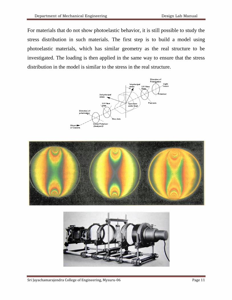
For materials that do not show photoelastic behavior, it is still possible to study the

stress distribution in such materials. The first step is to build a model using

photoelastic materials, which has similar geometry as the real structure to be

investigated. The loading is then applied in the same way to ensure that the stress

distribution in the model is similar to the stress in the real structure.



Experiment # 9

GYROSCOPE

AIM: To study the gyroscopic behavior of rotating masses and verify the gyroscopic

relationship.

Apparatus: Gyroscope, weights, stop watch, tachometer, spirit level

Fig. 10: Schematic representation of Gyroscope axis and aircraft

Theory: For theory answer the following questions

1. Write a short note on gyroscope.

2. What do you understand by gyroscopic couple? Derive a formula for its magnitude.

3. Explain the application of gyroscopic principles to aircrafts.

4. Discuss the effect of the gyroscopic couple on a two wheeled vehicle when taking a turn.

The earliest observation and studies on gyroscopic phenomenon carried out during Newton‟s

time. These were made in the context of the motion of our planet which in effect in a massive

gyroscopic. The credit of the mathematical foundation of the principles of gyroscopic motion

goes to Euler who derived at set of dynamic equation relating applied mechanics and moment

inertia, angular acceleration and angular velocity in many machines, the rotary components are

forced to turn about their axis other than their own axis of rotation and gyroscopic effects are

thus setup. The gyroscopes are used in ships to minimize the rolling & pitching effects of water.

A Gyroscope is a spinning body mounted universally to turn with an angular velocity of

precession in a direction at right angles to the direction of the moment causing it but its center of

gravity will be in a fixed position.

The gyroscope has 2 degrees of freedom. The first axis is OX called spin axis on which the body

is spinning. The second axis is OY called Torque axis. Third axis OA is called precession axis on

which the body moves opposing the original motion. All the 3 axis are mutually perpendicular.

Such a combined effect is known as Gyroscopic effect.



The analyses of gyroscopic principles are based on Newton‟s Laws of Motion and inertia. When

the rotor is spinned, the gyroscope exhibits the following two important characteristics:

1. Gyroscopic Inertia 2. Precession

Applications: The gyroscopic principle is used in an instrument or toy known as gyroscope. The

gyroscopes are installed in ships in order to minimize the rolling and pitching effects of waves.

They are also used in aeroplanes, monorail cars, gyrocompasses etc.

Gyroscopic Inertia: I = 1

2m𝑟2 =

1

2

𝜔𝑑

𝑔(𝐷

2) ^2 Kg-𝑚2

Where, m= mass of disc

𝑊𝑑 = wt of disc

D= dia of disc

Precession: When a force is applied to the gyroscope about the horizontal axis it may be found

that the applied force meets with resistance and that the gyro, instead of turning about the

horizontal axis, turns about its vertical axis and vice versa. It follows right hand thumb rule. Thus

the change in direction of plane of rotation of rotor is known as precession.

Velocity of Spin:

𝜔 =2𝜋𝑛

60 𝑟𝑎𝑑/𝑠 Where n = speed of motor in rpm

Velocity of Precession:

𝜔𝒑 =

𝑑𝜃

𝑑𝑡

= 𝝅𝜽

𝟏𝟖𝟎 rad/s Where 𝜃 = angle of precession, t= time for precession

Gyroscopic Couple: The couple generated due to change in direction of angular velocity of

rotor is called gyroscopic couple.

𝐶𝑔 = I𝜔𝜔𝑝 , N-m

Applied Torque: The torque applied to change the direction of angular velocity rotor is called

applied torque.

𝐶𝑎 = W.a. Where W = wt placed in the wt. stud, a= its distance from center of disc.

Angular momentum: C = I𝜔

Effect of the Gyroscopic Couple on an Aeroplane:

1. When the aeroplane takes a right turn under similar conditions. The effect of the reactive

gyroscopic couple will be to dip the nose and raise the tail of the aeroplane.

2. When the engine or propeller rotates in anticlockwise direction when viewed from the rear or

tail end and the aeroplane takes a left turn, then the effect of reactive gyroscopic couple will

be to dip the nose and raise the tail of the aeroplane.

3. When the aeroplane takes a right turn under similar conditions as mentioned in note 2 above,

the effect of reactive gyroscopic couple will be to raise the nose and dip the tail of the

aeroplane.



4. When the engine or propeller rotates in clockwise direction when viewed from the front and

the aeroplane takes a left turn, then the effect of reactive gyroscopic couple will be to raise

the tail and dip the nose of the aeroplane.

5. When the aeroplane takes a right turn under similar conditions as mentioned in note 4 above,

the effect of reactive gyroscopic couple will be to raise the nose and dip the tail of the

aeroplane.

The effect of gyroscopic couple on the naval ship in the following three cases :

1- Steering 2- Pitching and 3- Rolling

APPLICATIONS: The gyroscopic principle is used in an instrument or toy known as

gyroscope. The gyroscopes are installed in ships in order to minimize the rolling and pitching

effects of waves. They are also used in aeroplanes, monorail cars, gyrocompasses etc.

Effect of the Gyroscopic Couple on a Naval ship during Steering:-

1. When the ship steers to the right under similar conditions as discussed above, the effect of

the reactive gyroscopic couple will be to raise the stern and lower the bow.

2. When the rotor rotates in the anticlockwise direction, when viewed from the stern and the

ship is steering to the left, then the effect of reactive gyroscopic couple will be to lower the

bow and raise the stern.

3. When the ship is steering to the right under similar conditions as discussed in note 2 above,

then the effect of reactive gyroscopic couple will be to raise the bow and lower the stern.

4. When the rotor rotates in the clockwise direction when viewed from the bow or fore end and

the ship is steering to the left, then the effect of reactive gyroscopic couple will be to raise the

stern and lower the bow.

5. When the ship is steering to the right under similar conditions as discussed in note 4 above,

then the effect of reactive gyroscopic couple will be to raise the bow and lower the stern.

6. The effect of the reactive gyroscopic couple on a boat propelled by a turbine taking left or

right turn is similar as discussed above.

Effect of the Gyroscopic Couple on a Naval ship during Pitching:-

1. The effect of the gyroscopic couple is always given on specific position of the axis of spin,

i.e. whether it is pitching downwards or upwards.

2. The pitching of a ship produces forces on the bearings which act horizontally and

perpendicular to the motion of the ship.

3. The maximum gyroscopic couple tends to shear the holding-down bolts.

4. The angular acceleration during pitching.

α = d2θ/dt

2 = -Φ(ω1)

2 sin ω1t (Differentiating dθ/dt with respect to t)



The angular acceleration is maximum, if sin ω1t = 1

Therefore Maximum angular acceleration during pitching,

αmax = Φ(ω1)2

Effect of the Gyroscopic Couple on a Naval ship during Rolling:- We know that, for the

effect of gyroscopic couple to occur, the axis of precession should always be perpendicular to the

axis of spin. If, however, the axis of precession becomes parallel to the axis of spin, there will be

no effect of the gyroscopic couple acting on the body of the ship.

In case of rolling of a ship, the axis of precession (i.e. longitudinal axis) is always parallel to the

axis of spin for all positions. Hence, there is no effect of the gyroscopic couple acting on the

body of a ship.

Procedure of conduction of experiment:

1. Connect the motor of the gyroscope to an A.C. supply through dimmer stat.

2. Using spirit level, check the rotor for vertical position. Adjust the balance weight slightly if

required using the bottom clamp screws.

3. Set the dimmer at zero position and put ON the supply.

4. Start the motor by applying the voltage of around 170(for instant build up of voltage) and

then reduce gradually.

5. Adjust the rotor speed if required

6. Note down the rotor speed with the help of a tachometer when it becomes steady.

7. Place the required wt. on the wt. stud and at the same instant start the stop watch. Note down

the time required for degree of precession.

8. Repeat the procedure for different weights and precessions.

9. Measure and record the distance between the center of the disc and center of weight stud.

10. Tabulate the results.

11. Determine and compare the gyroscopic couple with that of applied torque and plot the

following curves:

i. Calibration curve ii. Gyroscopic couple Vs Precession.

Observations:

Rotor Diameter = 245 mm

Rotor thickness = 10 mm

M.I. of all Rotating Parts = 0.02986 Nm- sec

2



Distance from centre of Disc

to Centre of Dead Weights = 0.155 m

Motor speed Max = 6000 rpm

Speed of

motor

N rpm

Applied

load W

Angle of

precession

Degrees

Time taken

for

precession

„t‟ Sec

Angular

velocity

rad / s

Torque

applied

T Nm

Experiment

velocity of

precession

Pe rad / s

Theoretical

velocity of

precession

PT

rad / s

Kg N

60

60

60

60

Specimen calculations:

Angular Velocity of rotor 60

2 N

Gyroscopic couple (or) Torque Applied rWT N-m

Experimental Velocity of precision, t

Pe

180

rad/sec

Theoretical Velocity of Precision,

I

TPt rad/sec

Result:

Percentage error between applied torque and gyroscopic couple is: ____________

jss mahavidyapeetha jss science & technology … · department of mechanical engineering design...

Documents