julia: a fresh approach to numerical computing · julia: a fresh approach to numerical computing 67...

SIAM REVIEW c© 2017 Society for Industrial and Applied MathematicsVol. 59, No. 1, pp. 65–98

Julia: A Fresh Approach toNumerical Computing∗

Jeff Bezanson†

Alan Edelman‡

Stefan Karpinski§

Viral B. Shah†

Abstract. Bridging cultures that have often been distant, Julia combines expertise from the diversefields of computer science and computational science to create a new approach to numericalcomputing. Julia is designed to be easy and fast and questions notions generally held tobe “laws of nature” by practitioners of numerical computing:

1. High-level dynamic programs have to be slow.2. One must prototype in one language and then rewrite in another language for speed

or deployment.3. There are parts of a system appropriate for the programmer, and other parts that are

best left untouched as they have been built by the experts.

We introduce the Julia programming language and its design—a dance between special-ization and abstraction. Specialization allows for custom treatment. Multiple dispatch,a technique from computer science, picks the right algorithm for the right circumstance.Abstraction, which is what good computation is really about, recognizes what remains thesame after differences are stripped away. Abstractions in mathematics are captured ascode through another technique from computer science, generic programming.

Julia shows that one can achieve machine performance without sacrificing human con-venience.

Key words. Julia, numerical, scientific computing, parallel

AMS subject classifications. 68N15, 65Y05, 97P40

DOI. 10.1137/141000671

Contents

1 Scientific Computing Languages: The Julia Innovation 661.1 Julia Architecture and Language Design Philosophy . . . . . . . . . . 67

∗Received by the editors December 18, 2014; accepted for publication (in revised form) December16, 2015; published electronically February 7, 2017.

http://www.siam.org/journals/sirev/59-1/100067.htmlFunding: This work received financial support from the MIT Deshpande Center for Technological

Innovation, the Intel Science and Technology Center for Big Data, the DARPA XDATA program, theSingapore MIT Alliance, an Amazon Web Services grant for JuliaBox, NSF awards CCF-0832997,DMS-1016125, and DMS-1312831, VMware Research, a DOE grant with Dr. Andrew Gelman ofColumbia University for petascale hierarchical modeling, grants from Saudi Aramco thanks to AliDogru and Shell Oil thanks to Alon Arad, and a Citibank grant for High Performance Banking DataAnalysis, Chris Mentzel, and the Gordon and Betty Moore Foundation.†Julia Computing, Inc. ([email protected], [email protected]).‡CSAIL and Department of Mathematics, Massachusetts Institute of Technology, Cambridge, MA

02139 ([email protected]).§New York University, New York, NY 10012, and Julia Computing, Inc. (stefan@juliacomputing.

com).

65

http://www.siam.org/journals/s

mailto:[email protected]





66 JEFF BEZANSON, ALAN EDELMAN, STEFAN KARPINSKI, AND VIRAL B. SHAH

2 A Taste of Julia 682.1 A Brief Tour . . . . . . . . . . . . . . . . . . . . . . . . . . . . . . . . 682.2 An Invaluable Tool for Numerical Integrity . . . . . . . . . . . . . . . 722.3 The Julia Community . . . . . . . . . . . . . . . . . . . . . . . . . . . 74

3 Writing Programs With and Without Types 743.1 The Balance between Human and the Computer . . . . . . . . . . . . 743.2 Julia’s Recognizable Types . . . . . . . . . . . . . . . . . . . . . . . . 743.3 User’s Own Types Are First Class Too . . . . . . . . . . . . . . . . . . 753.4 Vectorization: Key Strengths and Serious Weaknesses . . . . . . . . . 763.5 Type Inference Rescues “For Loops” and So Much More . . . . . . . . 78

4 Code Selection: Run the Right Code at the Right Time 784.1 Multiple Dispatch . . . . . . . . . . . . . . . . . . . . . . . . . . . . . 794.2 Code Selection from Bits to Matrices . . . . . . . . . . . . . . . . . . . 81

4.2.1 Summing Numbers: Floats and Ints . . . . . . . . . . . . . . . 814.2.2 Summing Matrices: Dense and Sparse . . . . . . . . . . . . . . 82

4.3 The Many Levels of Code Selection . . . . . . . . . . . . . . . . . . . . 834.4 Is “Code Selection” Traditional Object Oriented Programming? . . . . 854.5 Quantifying the Use of Multiple Dispatch . . . . . . . . . . . . . . . . 864.6 Case Study for Numerical Computing . . . . . . . . . . . . . . . . . . 87

4.6.1 Determinant: Simple Single Dispatch . . . . . . . . . . . . . . . 884.6.2 A Symmetric Arrow Matrix Type . . . . . . . . . . . . . . . . . 89

5 Leveraging Design for High Performance Libraries 905.1 Integer Arithmetic . . . . . . . . . . . . . . . . . . . . . . . . . . . . . 905.2 A Powerful Approach to Linear Algebra . . . . . . . . . . . . . . . . . 91

5.2.1 Matrix Factorizations . . . . . . . . . . . . . . . . . . . . . . . 915.2.2 User-Extensible Wrappers for BLAS and LAPACK . . . . . . . 92

5.3 High Performance Polynomials and Special Functions with Macros . . 935.4 Easy and Flexible Parallelism . . . . . . . . . . . . . . . . . . . . . . . 945.5 Performance Recap . . . . . . . . . . . . . . . . . . . . . . . . . . . . . 96

6 Conclusion 97

References 97

1. Scientific Computing Languages: The Julia Innovation. The original nu-merical computing language was Fortran, short for “Formula Translating System,”released in 1957. Since those early days, scientists have dreamed of writing high-level,generic formulas and having them translated automatically into low-level, efficientcode, tailored to the particular data types they need to apply the formulas to. For-tran made historic strides toward the realization of this dream, and its dominance inso many areas is a testament to its success.

The landscape of computing has changed dramatically over the years. Modernscientific computing environments such as Python [34], R [12], Mathematica [21],Octave [25], MATLAB [22], and Scilab [10], to name a few, have grown in popularityand fall under the general category known as dynamic languages or dynamically typedlanguages. In these programming languages, programmers write simple, high-levelcode without any mention of types like int, float, or double that pervade staticallytyped languages such as C and Fortran.

JULIA: A FRESH APPROACH TO NUMERICAL COMPUTING 67

Many researchers today work in dynamic languages. Still, C and Fortran remainthe gold standard for performance for computationally intensive problems. As muchas the dynamic language programmer misses out on performance, though, the C andFortran programmer misses out on productivity. An unfortunate outcome is thatthe most challenging areas of numerical computing have benefited the least fromthe increased abstraction and productivity offered by higher-level languages. Theconsequences have been more serious than many realize.

Julia’s innovation lies in its combination of productivity and performance. Newusers want a quick explanation as to why Julia is fast and want to know whethersomehow the same “magic dust” could also be sprinkled on their favorite traditionalscientific computing language. Julia is fast because of careful language design andthe right combination of carefully chosen technologies that work very well with eachother. This article demonstrates some of these technologies using a number of exam-ples. Celeste serves as an example for readers interested in a large-scale applicationthat leverages 8,192 cores on the Cori Supercomputer at Lawrence Berkeley NationalLaboratory [28].

Users interact with Julia through a standard REPL (real-eval-print loop environ-ment such as Python, R, or MATLAB), by collecting commands in a .jl file, or bytyping directly in a Jupyter (JUlia, PYThon, R) notebook [15, 30]. We invite thereader to follow along at http://juliabox.com using Jupyter notebooks or by down-loading Julia from http://julialang.org/downloads.

1.1. Julia Architecture and Language Design Philosophy. Many popular dy-namic languages were not designed with the goal of high performance in mind. Afterall, if you wanted really good performance you would use a static language, or so saidthe popular wisdom. Only with the increasing need in the day-to-day life of scientificprogrammers for simultaneous productivity and performance has the need for highperformance dynamic languages become pressing. Unfortunately, retrofitting an ex-isting slow dynamic language for high performance is almost impossible, specificallyin numerical computing ecosystems. This is because numerical computing requiresperformance-critical numerical libraries, which invariably depend on the details of theinternal implementation of the high-level language, thereby locking in those internalimplementation details. For example, you can run Python code much faster than thestandard CPython implementation using the PyPy just-in-time (JIT) compiler, butPyPy is currently incompatible with NumPy and the rest of SciPy.

Another important point is that just because a program is available in C orFortran, it may not run efficiently from the high-level language.

The best path to a fast, high-level system for scientific and numerical computing isto make the system fast enough that all of its libraries can be written in the high-levellanguage in the first place. The JuMP.jl [20] package for mathematical programmingand the Convex.jl [33] package for convex optimization are great examples of thesuccess of this approach—in each case the entire library is written in Julia and usesmany Julia language features described in this article.

The Two Language Problem. As long as the developers’ language is harder tograsp than the users’ language, numerical computing will always be hindered. Thisis an essential part of the design philosophy of Julia: all basic functionality must bepossible to implement in Julia—never force the programmer to resort to using C orFortran. Julia solves the two language problem. Basic functionality must be fast:integer arithmetic, for loops, recursion, floating-point operations, calling C functions,and manipulating C-like structs. While these features are not only important for

http://juliabox.com

http://julialang.org/downloads


numerical programs, without them you certainly cannot write fast numerical code.“Vectorization languages” like Python+NumPy, R, and MATLAB hide their for loopsand integer operations, but they are still there, inside the C and Fortran, lurkingbeneath the thin veneer. Julia removes this separation entirely, allowing the high-levelcode to “just write a for loop” if that happens to be the best way to solve a problem.

We believe that the Julia programming language fulfills much of the Fortrandream: automatic translation of formulas into efficient executable code. It allowsprogrammers to write clear, high-level, generic and abstract code that closely re-sembles mathematical formulas, yet produces fast, low-level machine code that hastraditionally only been generated by static languages.

Julia’s ability to combine these levels of performance and productivity in a singlelanguage stems from the choice of a number of features that work well with each other:

1. An expressive type system, allowing optional type annotations (section 3).2. Multiple dispatch using these types to select implementations (section 4).3. Metaprogramming for code generation (section 5.3).4. A dataflow type inference algorithm allowing types of most expressions to be

inferred [2, 4].5. Aggressive code specialization against run-time types [2, 4].6. JIT compilation [2, 4] using the LLVM compiler framework [18], which is also

used by a number of other compilers such as Clang [6] and Apple’s Swift [32].7. Julia’s carefully written libraries that leverage the language design, i.e., points

1 through 6 above (section 5).Points 1, 2, and 3 above are features especially for the human user, and they are

the focus of this paper. For details about the features related to language implemen-tation and internals such as those in points 4, 5, and 6, we direct the reader to ourearlier work [2, 4]. The feature in point 7 brings everything together to enable thebuilding of high performance computational libraries in Julia.

Although a sophisticated type system is made available to the programmer, itremains unobtrusive in the sense that one is never required to specify types, andneither are type annotations necessary for performance. Type information flows nat-urally through the program due to dataflow type inference.

In what follows, we describe the benefits of Julia’s language design for numeri-cal computing, allowing programmers to more readily express themselves while alsoobtaining performance.

2. A Taste of Julia.

2.1. A Brief Tour.

In[1]: A = rand(3,3) + eye(3) # Familiar Syntax

inv(A)

# The result of the final expression is displayed in Out[1]

Out[1]: 3x3 Array{Float64,2}:0.698106 -0.393074 -0.0480912

-0.223584 0.819635 -0.124946

-0.344861 0.134927 0.601952

The output from the Julia prompt says that A−1 is a two-dimensional matrix ofsize 3× 3 and contains double precision floating-point numbers.

Indexing of arrays is performed with brackets with index origin 1. It is also pos-sible to compute an entire array expression and then index into it, without assigning


the expression to a variable:

In[2]: x = A[1,2]

y = (A+2I)[3,3] # The [3,3] entry of A+2I

Out[2]: 2.601952

In Julia, I is a built-in representation of the identity matrix, without any explicitforming of the identity matrix as is commonly done using commands such as “eye.”(“eye,” a homonym of “I,” is used in such languages as MATLAB, Octave, Go’s matrixlibrary, Python’s NumPy, and Scilab.)

Julia has symmetric tridiagonal matrices as a special type. For example, we maydefine Gil Strang’s favorite matrix (the second-order difference matrix; see Figure 1)in a way that uses only O(n) memory.

Fig. 1 Gil Strang’s favorite matrix is strang(n) = SymTridiagonal(2*ones(n),-ones(n-1)). Juliaonly stores the diagonal and off-diagonal. (Picture taken in Gil Strang’s classroom.)

In[3]: strang(n) = SymTridiagonal(2*ones(n),-ones(n-1))

strang(7)

Out[3]: 7x7 SymTridiagonal{Float64}:2.0 -1.0 0.0 0.0 0.0 0.0 0.0

-1.0 2.0 -1.0 0.0 0.0 0.0 0.0

0.0 -1.0 2.0 -1.0 0.0 0.0 0.0

0.0 0.0 -1.0 2.0 -1.0 0.0 0.0

0.0 0.0 0.0 -1.0 2.0 -1.0 0.0

0.0 0.0 0.0 0.0 -1.0 2.0 -1.0

0.0 0.0 0.0 0.0 0.0 -1.0 2.0

A commonly used notation to express the solution x to the equation Ax = b isA\b. If Julia knows that A is a tridiagonal matrix, it uses an efficient O(n) algorithm:

In[4]: strang(8)\ones(8)


Out[4]: 8-element Array{Float64,1}:4.0

7.0

9.0

10.0

10.0

9.0

7.0

4.0

Note the Array{ElementType,dims} syntax. In the above example, the elementsare 64-bit floats or Float64’s. The 1 indicates it is a one-dimensional vector.

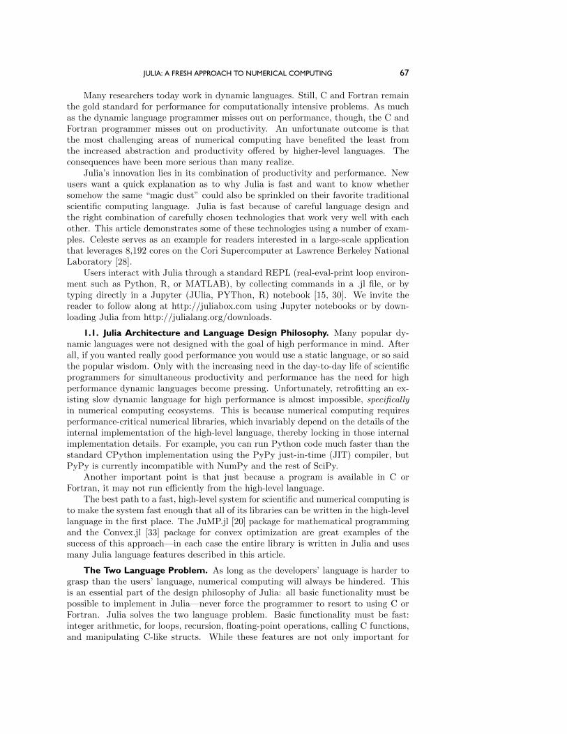
Consider the sorting of complex numbers. Sometimes it is handy to have a sortthat generalizes the real sort. This can all be done by sorting first by the real part,and where there are ties, sort by the imaginary part. Other times it is handy to usethe polar representation, which sorts by radius then by angle. By default, complexnumbers are incomparable in Julia.

If a numerical computing language “hardwires” its sort to be one or the other,it misses an opportunity. A sorting algorithm need not depend on the details ofwhat is being compared or how it is done so. One can abstract away these details,thereby enabling the reuse of a sorting algorithm for many different situations. Onecan specialize later. Thus, alphabetizing strings, sorting real numbers, and sortingcomplex numbers in two or more ways can all be done using the same code.

In Julia, one can turn a complex number w into an ordered pair of real numbers (atuple of length 2) such as the Cartesian form (real(w),imag(w)) or the polar form(abs(w),angle(w)). Tuples are then compared lexicographically. The sort commandtakes an optional “less-than” operator, lt, which is used to compare elements whensorting.

In[5]: # Cartesian comparison sort of complex numbers

complex compare1(w,z) = (real(w),imag(w)) < (real(z),imag(z))

sort([-2,2,-1,im,1], lt = complex compare1 )

Out[5]: 5-element Array{Complex{Int64},1}:-2+0im

-1+0im

0+1im

1+0im

2+0im

In[6]: # Polar comparison sort of complex numbers

complex compare2(w,z) = (abs(w),angle(w)) < (abs(z),angle(z))

sort([-2,2,-1,im,1], lt = complex compare2)

Out[6]: 5-element Array{Complex{Int64},1}:1+0im

0+1im

-1+0im

2+0im

-2+0im


To be sure, experienced computer scientists tend to suspect that there is nothingnew under the sun. The C function qsort() takes a compar function, so there isnothing really new there. Python also has custom sorting with a key; MATLAB’ssort is more basic. The real contribution of Julia, as will be fleshed out further in thisarticle, is that its design allows custom sorting to be high performance, flexible, andcomparable with implementations that are often written in C.

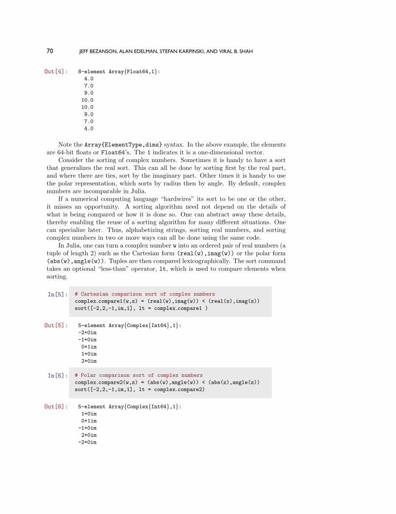
The next example that we have chosen for this introductory taste of Julia is aquick plot of Brownian motion, in two ways. The first uses the Python Matplotlibpackage for graphics, which is popular for users coming from Python or MATLAB.The second uses Gadfly.jl, another very popular package for plotting. Gadfly wasbuilt completely in Julia by Daniel Jones and was influenced by the much-admired“Grammar of Graphics” (see [36] and [35]).1 Many Julia users find Gadfly moreflexible and prefer its aesthetics. Julia plots can also be manipulated interactivelywith sliders and buttons using its Interact.jl package.2 The Interact.jl package webpage contains many examples of interactive visualizations.3

In[7]: Pkg.add("PyPlot") # Download the PyPlot package

using PyPlot # load the functionality into Julia

for i=1:5

y=cumsum(randn(500))

plot(y)

end

1See tutorial at http://gadflyjl.org2https://github.com/JuliaLang/Interact.jl3https://github.com/JuliaLang/Interact.jl/issues/36

http://gadflyjl.org

https://github.com/JuliaLang/Interact.jl

https://github.com/JuliaLang/Interact.jl/issues/36


In[8]: Pkg.add("Gadfly") # Download the Gadfly package

using Gadfly # load the functionality into Julia

n = 500

l = ["First", "Second", "Third"]

c = [colorant"yellow",colorant"cyan",colorant"magenta"]

p = [layer(x=1:n, y=cumsum(randn(n)), Geom.line,

Theme(default_color=i)) for i in c ]

labels=(Guide.xlabel("Time"),Guide.ylabel("Value"),

Guide.title("Brownian Motion Trials"),

Guide.manual_color_key("Legend", l, c))

Gadfly.plot(p...,labels...)

Time0 100 400 500

FirstSecondThird

Trial

Valu

e

-60

-40

-20

0

20

Brownian Motion Trials

300200

The ellipses on the last line of text above are known as a splat operator. Theelements of the vector p and the tuple labels are inserted individually as argumentsto the plot function.

2.2. An Invaluable Tool for Numerical Integrity. One popular feature of Juliais that it gives the user the ability to “kick the tires” of a numerical computation. Wethank Velvel Kahan for the sage advice4 concerning the importance of this feature.

The idea is simple: a good engineer tests his or her code for numerical stability. InJulia this can be done by changing the IEEE rounding modes. There are five modes tochoose from, yet most engineers silently choose only the RoundNearest mode defaultavailable in many numerical computing systems. If a difference is detected, one canalso run the computation in higher precision. Kahan [16] writes:

Can the effects of roundoff upon a floating-point computation be assessedwithout submitting it to a mathematically rigorous and (if feasible at all)time-consuming error-analysis? In general, No. . . .

4Personal communication, January 2013, in the Kahan home, Berkeley, California.


Though far from foolproof, rounding every inexact arithmetic operation(but not constants) in the same direction for each of two or three directionsbesides the default To Nearest is very likely to confirm accidentally exposedhypersensitivity to roundoff. When feasible, this scheme offers the bestBenefit/Cost ratio.

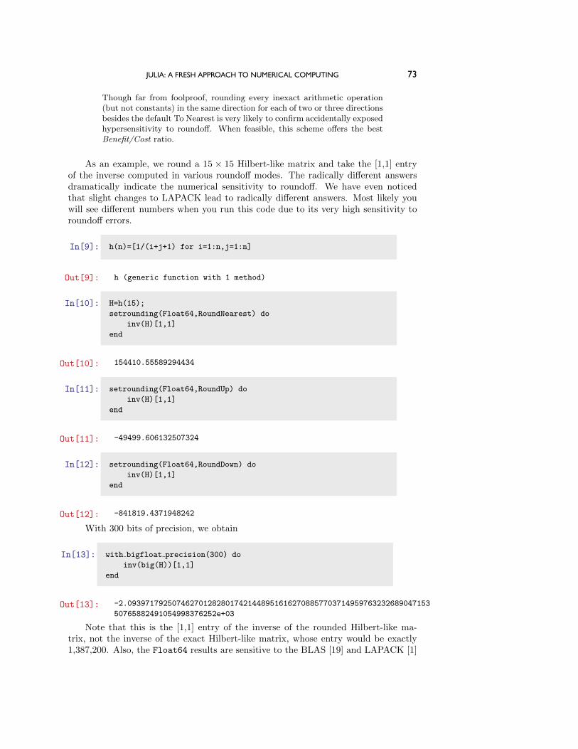
As an example, we round a 15 × 15 Hilbert-like matrix and take the [1,1] entryof the inverse computed in various roundoff modes. The radically different answersdramatically indicate the numerical sensitivity to roundoff. We have even noticedthat slight changes to LAPACK lead to radically different answers. Most likely youwill see different numbers when you run this code due to its very high sensitivity toroundoff errors.

In[9]: h(n)=[1/(i+j+1) for i=1:n,j=1:n]

Out[9]: h (generic function with 1 method)

In[10]: H=h(15);

setrounding(Float64,RoundNearest) do

inv(H)[1,1]

end

Out[10]: 154410.55589294434

In[11]: setrounding(Float64,RoundUp) do

inv(H)[1,1]

end

Out[11]: -49499.606132507324

In[12]: setrounding(Float64,RoundDown) do

inv(H)[1,1]

end

Out[12]: -841819.4371948242

With 300 bits of precision, we obtain

In[13]: with bigfloat precision(300) do

inv(big(H))[1,1]

end

Out[13]: -2.09397179250746270128280174214489516162708857703714959763232689047153

50765882491054998376252e+03

Note that this is the [1,1] entry of the inverse of the rounded Hilbert-like ma-trix, not the inverse of the exact Hilbert-like matrix, whose entry would be exactly1,387,200. Also, the Float64 results are sensitive to the BLAS [19] and LAPACK [1]


libraries, and may differ on different machines with different versions of Julia. Forextended precision, Julia uses the MPFR library [9].

2.3. The Julia Community. Julia has been under development since 2009, and apublic release was announced in February of 2012. It is an active open source projectwith over 500 contributors and is available under the MIT License [23] for open sourcesoftware. Over 2 million unique visitors have visited the Julia website since then, andJulia has now been adopted as a teaching tool in dozens of universities around theworld.5 The community has contributed over 1200 Julia packages. While it was nur-tured at the Massachusetts Institute of Technology, it is really the contributions fromexperts around the world that make it a joy to use for numerical computing. It isalso recognized as a general purpose computing language, unlike traditional numericalcomputing systems, allowing it to be used not only to prototype numerical algorithms,but also to deploy those algorithms and even serve results to the rest of the world. Agreat example of this is Shashi Gowda’s Escher.jl package,6 which makes it possiblefor Julia programmers to build beautiful interactive websites in Julia and serve up theresults of a Julia computation from the web server, without any knowledge of HTMLor JavaScript. Another such example is “Sudoku-as-a-Service,”7 by Iain Dunning,where a Sudoku puzzle is solved using the optimization capabilities of the JuMP.jl Ju-lia package [20] and made available as a web service. This is exactly why Julia is beingincreasingly deployed in production environments in businesses, as is seen in varioustalks at JuliaCon.8 These use cases utilize Julia’s capabilities not only for mathemat-ical computation, but for building web APIs, database access, and much more.

3. Writing Programs With and Without Types.

3.1. The Balance between Human and the Computer. Graydon Hoare, authorof the Rust programming language [29], defined programming languages succinctly inan essay on Interactive Scientific Computing [11]:

Programming languages are mediating devices, interfaces that try to strikea balance between human needs and computer needs. Implicit in that isthe assumption that human and computer needs are equally important, orneed mediating.

A program consists of data and operations on data. Data is not just the input file,but everything that is held—an array, a list, a graph, a constant—during the life of theprogram. The more the computer knows about this data, the better it is at executingoperations on it. Types are exactly this metadata. Describing this metadata, thetypes, takes real effort for the human. Statically typed languages such as C andFortran are at one extreme, where all types must be defined and are statically checkedduring the compilation phase. The result is excellent performance. Dynamically typedlanguages dispense with type definitions, which leads to greater productivity but lowerperformance as the compiler and the runtime cannot benefit from the type informationthat is essential to producing fast code. Can we strike a balance between the human’spreference to avoid types and the computer’s need to know?

3.2. Julia’s Recognizable Types. Many users of Julia may never need to knowabout types for performance. Julia’s type inference system often does all the work,giving performance without type declarations.

5http://julialang.org/community6https://github.com/shashi/Escher.jl7http://iaindunning.com/2013/sudoku-as-a-service.html8http://www.juliacon.org

http://julialang.org/community

http://www.juliacon.org


Julia’s design allows for the gradual learning of concepts, where users start in amanner that is familiar to them and, over time, learn to structure programs in the“Julian way”—a term that implies well-structured readable high performance Juliacode. Julia users coming from other numerical computing environments have a notionthat data may be represented as matrices that may be dense, sparse, symmetric,triangular, or of some other kind. They may also, though not always, know thatelements in these data structures may be single or double precision floating-pointnumbers, or integers of a specific width. In more general cases, the elements withindata structures may be other data structures. We introduce Julia’s type system usingmatrices and their number types:

In[14]: rand(1,2,1)

Out[14]: 1x2x1 Array{Float64,3}:[ :, :, 1] =

0.789166 0.652002

In[15]: [1 2; 3 4]

Out[15]: 2x2 Array{Int64,2}:1 2

3 4

In[16]: [true; false]

Out[16]: 2-element Array{Bool,1}:true

false

We see a pattern in the examples above. Array{T,ndims} is the general form ofthe type of a dense array with ndims dimensions whose elements themselves have aspecific type T, which is of type double precision floating point in the first example,a 64-bit signed integer in the second, and a boolean in the third example. Therefore,Array{T,1} is a one-dimensional vector (first class objects in Julia) with element typeT and Array{T,2} is the type for two-dimensional matrices.

It is useful to think of an array as a generic N-dimensional object that may containelements of any type T. Thus, T is a type parameter for an array that can take on manydifferent values. Similarly, the dimensionality of the array ndims is also a parameterfor the array type. This generality makes it possible to create arrays of arrays. Forexample, using Julia’s array comprehension syntax, we create a two-element vectorcontaining 2× 2 identity matrices:

In[17]: a = [eye(2) for i=1:2]

Out[17]: 2-element Array{Array{Float64,2},1}:

3.3. User’s Own Types Are First Class Too. Many dynamic languages for nu-merical computing have traditionally contained an asymmetry, with built-in typeshaving much higher performance than any user-defined types. This is not the case


with Julia, where there is no meaningful distinction between user-defined and “built-in” types.

We have mentioned so far a few number types and two matrix types: Array{T,2},the dense array with element type T, and SymTridiagonal{T}, the symmetric tridi-agonal with element type T. There are also other matrix types for other structures in-cluding SparseMatrixCSC (compressed sparse columns), Hermitian, Triangular, Bidi-agonal, and Diagonal. Julia’s sparse matrix type has an added flexibility, that it cango beyond storing just numbers as nonzeros, and can instead store any other Juliatype as well. The indices in SparseMatrixCSC can also be represented as integers ofany width (16-bit, 32-bit, or 64-bit). All these different matrix types, available asbuilt-in types to a user downloading Julia, are implemented completely in Julia andare in no way any more or less special than any other types a user may define in theirown program.

For demonstration purposes, we now create a symmetric arrow matrix type thatcontains a diagonal and the first row A[1,2:n]. Oce could also throw an ArgumentEr-ror if the ev vector was not one shorter in length than the dv vector.

In[18]: # Type Parameter Example (Parameter T)

# Define a Symmetric Arrow Matrix Type with elements of type T

type SymArrow{T}dv::Vector{T} # diagonal

ev::Vector{T} # 1st row[2:n]

end

# Create your first Symmetric Arrow Matrix

S = SymArrow([1,2,3,4,5],[6,7,8,9])

Out[18]: SymArrow{Int64}([1,2,3,4,5],[6,7,8,9])

The parameter in the array refers to the type of each element of the array. Codecan and should be written independently of the type of each element.

In section 4.6.2, we develop the symmetric arrow example much further. TheSymArrow matrix type contains two vectors, one each for the diagonal and the first row,and these vectors contain elements of type T. In the type definition, the type SymArrowis parametrized by the type of the storage element T. By doing so, we have created ageneric type, which refers to a universe of all arrow matrices containing elements ofall types. The matrix S is an example where T is Int64. When we write functionsin section 4.6.2 that operate on arrow matrices, those functions themselves will begeneric and applicable to the entire universe of arrow matrices we have defined here.

Julia’s type system allows for abstract types, concrete “bits” types, compositetypes, and immutable composite types. All of these types can have parameters andusers may even write programs using unions of them. We refer the reader to fulldetails about Julia’s type system in the types chapter in the Julia manual.9

3.4. Vectorization: Key Strengths and Serious Weaknesses. Users of tradi-tional high-level computing languages know that vectorization improves performance.Do most users know exactly why vectorization is so useful? It is precisely because,

9See http://docs.julialang.org/en/latest/manual/types/

http://docs.julialang.org/en/latest/manual/types/


by vectorizing, the user has promised the computer that the type of an entire vectorof data matches the very first element. This is an example where users are willingto provide type information to the computer without even knowing that is what theyare doing. Hence, it is an example of a strategy that balances the computer’s needswith the human’s.

From the computer’s viewpoint, vectorization means that operations on datahappen largely in sections of the code where types are known to the runtime system.The runtime has no idea about the data contained in an array until it encountersthe array. Once encountered, the type of the data within the array is known, andthis knowledge is used to execute an appropriate high performance kernel. Of course,what really occurs at runtime is that the system figures out the type and then reusesthat information through the length of the array. As long as the array is not toosmall, all the extra work incurred in gathering type information and acting upon itat run time is amortized over the entire operation.

The downside of this approach is that the user can achieve high performanceonly with built-in types. User-defined types end up being dramatically slower. Therestructuring for vectorization is often unnatural, and at times not possible. Weillustrate this with an example of a cumulative sum computation. Note that due tothe size of the problem, the computation is memory bound, and one does not observethe case with complex arithmetic to be twice as slower than the real case, even thoughit is performing twice as many floating point operations.

In[19]: # Sum prefix (cumsum) on vector w with elements of type T

function prefix{T}(w::Vector{T})for i=2:size(w,1)

w[i]+=w[i-1]

end

w

end

We execute this code on a vector of double precision real numbers and doubleprecision complex numbers and observe something that may seem remarkable: similarrun times in each case.

In[20]: x = ones(1 000 000)

@time prefix(x)

y = ones(1 000 000) + im*ones(1 000 000)

@time prefix(y);

Out[20]: elapsed time: 0.003243692 seconds (80 bytes allocated)

elapsed time: 0.003290693 seconds (80 bytes allocated)

This simple example is difficult to vectorize, and hence is often provided as a built-in function in many numerical computing systems. In Julia, the implementation isvery similar to the snippet of code above and runs at speeds similar to C. While Juliausers can write vectorized programs as in any other dynamic language, vectorizationis not a prerequisite for performance. This is because Julia strikes a different balance


between the human and the computer when it comes to specifying types. Julia allowsoptional type annotations, which are essential when writing libraries but not for end-user programs that are exploring algorithms or a dataset.

Generally, in Julia, type annotations are not used for performance, but purelyfor code selection (see section 4). If the programmer annotates their program withtypes, the Julia compiler will use that information. However, in general, user codeoften includes minimal or no type annotations, and the Julia compiler automaticallyinfers the types.

3.5. Type Inference Rescues “For Loops” and So Much More. A key compo-nent of Julia’s ability to combine performance with productivity in a single languageis its implementation of dataflow type inference [24, 17, 4]. Unlike type inference al-gorithms for static languages, this algorithm is tailored to the way dynamic languageswork: the typing of code is determined by the flow of data through it. The algorithmworks by walking through a program, starting with the types of its input values, and“abstractly interpreting” it: instead of applying the code to values, it applies thecode to types, following all branches concurrently and tracking all possible states theprogram could be in, including all the types each expression could assume.

The dataflow type inference algorithm allows programs to be automatically an-notated with type bounds without forcing the programmer to explicitly specify types.Yet, in dynamic languages it is possible to write programs which inherently cannot beconcretely typed. In such cases, dataflow type inference provides what bounds it can,but these may be trivial and useless—i.e., they may not narrow down the set of possi-ble types for an expression at all. However, the design of Julia’s programming modeland standard library are such that a majority of expressions in typical programs canbe concretely typed.

A lesson of the numerical computing languages is that one must learn to vectorizeto get performance. The mantra is “for loops” are bad, vectorization is good. Indeedone can find the following mantra on p.72 of the 1998 Getting Started with MATLABmanual (and other editions):

Experienced MATLAB users like to say “Life is too short to spend writingfor loops.”

It is not that “for loops” are inherently slow in themselves. The slowness comesfrom the fact that in the case of most dynamic languages, the system does not haveaccess to the types of the variables within a loop. Since programs often spend much oftheir time doing repeated computations, the slowness of a particular operation due tolack of type information is magnified inside a loop. This leads to users often talkingabout “slow for loops” or “loop overhead.”

4. Code Selection: Run the Right Code at the Right Time. Code selection orcode specialization from one point of view is the opposite of the code reuse enabledby abstraction. Ironically, viewed another way, it enables abstraction. Julia allowsusers to overload function names and select code based on argument types. This canhappen at the highest and lowest levels of the software stack. Code specialization letsus optimize for the details of the case at hand. Code abstraction lets calling codes,even those not yet written or perhaps not even imagined, work on structures thatmay not have been envisioned by the original programmer.


We see this as the ultimate realization of the famous 1908 quip that

Mathematics is the art of giving the same name to different things.10

by noted mathematician Henri Poincare.In the next section we provide examples of how “plus” can apply to so many

objects, such as floating-point numbers or integers. It can also apply to sparse anddense matrices. Another example is the use of the same name, “det,” for determinant,for the very different algorithms that apply to very different matrix structures. The useof overloading not only for single argument functions, but also for multiple argumentfunctions, is already a powerful abstraction.

4.1. Multiple Dispatch. Multiple dispatch is the selection of a function imple-mentation based on the types of each argument of the function. It is not only a nicenotation to remove a long list of “case” statements, but is also part of the reason forJulia’s speed. It is expressed in Julia by annotating the type of a function argumentin a function definition with the following syntax: argument::Type.

Mathematical notations that are often used in print can be difficult to employ inprograms. For example, we can teach the computer some natural ways to multiplynumbers and functions. Suppose that a and t are scalars, and f and g are functions,and we wish to define the following operations:

1. Number x Function = scale output: a ∗ g is the function that takes xto a ∗ g(x);

2. Function x Number = scale argument : f ∗ t is the function that takesx to f(tx); and

3. Function x Function = composition of functions: f ∗ g is the functionthat takes x to f(g(x)).

If you were a mathematician who does not program, you would not see the fuss.If, however, you wanted to implement this in your favorite computer language, youmight immediately see the benefit. In Julia, multiple dispatch makes all three uses of

10A few versions of Poincare’s quote are relevant to Julia’s power of abstraction and numericalcomputing. They are worth pondering:

It is the harmony of the different parts, their symmetry, and their happy adjustment; itis, in a word, all that introduces order, all that gives them unity, that enables us to obtaina clear comprehension of the whole as well as of the parts. Elegance may result fromthe feeling of surprise caused by the unlooked-for occurrence of objects not habituallyassociated. In this, again, it is fruitful, since it discloses thus relations that were untilthen unrecognized. Mathematics is the art of giving the same names to different things.

(http://www.nieuwarchief.nl/serie5/pdf/naw5-2012-13-3-154.pdf)

One example has just shown us the importance of terms in mathematics; but I couldquote many others. It is hardly possible to believe what economy of thought, as Machused to say, can be effected by a well-chosen term. I think I have already said somewherethat mathematics is the art of giving the same name to different things. It is enoughthat these things, though differing in matter, should be similar in form, to permit of theirbeing, so to speak, run in the same mould. When language has been well chosen, one isastonished to find that all demonstrations made for a known object apply immediately tomany new objects: nothing requires to be changed, not even the terms, since the nameshave become the same.

(http://www-history.mcs.st-andrews.ac.uk/Extras/Poincare Future.html)

http://www.nieuwarchief.nl/serie5/pdf/naw5-2012-13-3-154.pdf

http://www-history.mcs.st-andrews.ac.uk/Extras/Poincare_Future.html


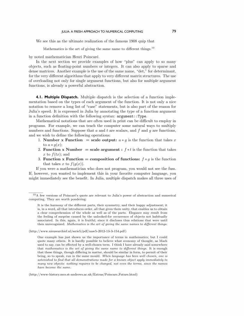
Fig. 2 Gauss quote hanging from the ceiling of the longstanding Boston Museum of Science Math-ematica Exhibit.

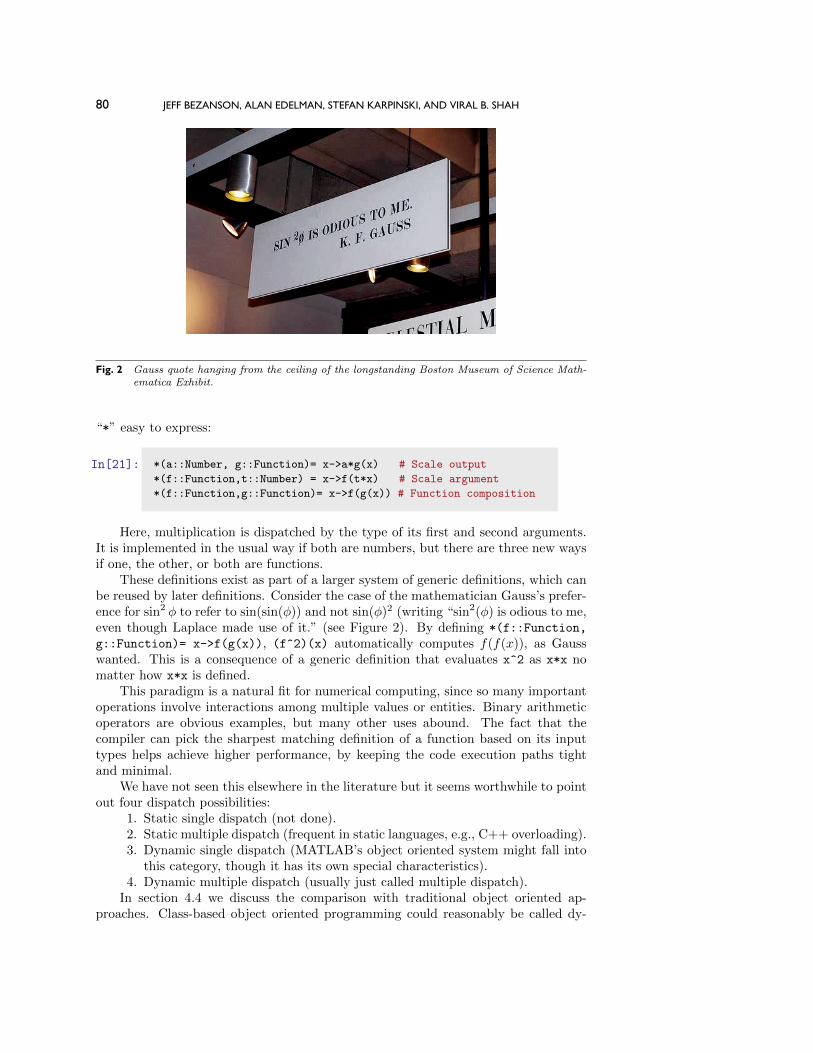
“*” easy to express:

In[21]: *(a::Number, g::Function)= x->a*g(x) # Scale output

*(f::Function,t::Number) = x->f(t*x) # Scale argument

*(f::Function,g::Function)= x->f(g(x)) # Function composition

Here, multiplication is dispatched by the type of its first and second arguments.It is implemented in the usual way if both are numbers, but there are three new waysif one, the other, or both are functions.

These definitions exist as part of a larger system of generic definitions, which canbe reused by later definitions. Consider the case of the mathematician Gauss’s prefer-ence for sin2 φ to refer to sin(sin(φ)) and not sin(φ)2 (writing “sin2(φ) is odious to me,even though Laplace made use of it.” (see Figure 2). By defining *(f::Function,

g::Function)= x->f(g(x)), (f^2)(x) automatically computes f(f(x)), as Gausswanted. This is a consequence of a generic definition that evaluates x^2 as x*x nomatter how x*x is defined.

This paradigm is a natural fit for numerical computing, since so many importantoperations involve interactions among multiple values or entities. Binary arithmeticoperators are obvious examples, but many other uses abound. The fact that thecompiler can pick the sharpest matching definition of a function based on its inputtypes helps achieve higher performance, by keeping the code execution paths tightand minimal.

We have not seen this elsewhere in the literature but it seems worthwhile to pointout four dispatch possibilities:

1. Static single dispatch (not done).2. Static multiple dispatch (frequent in static languages, e.g., C++ overloading).3. Dynamic single dispatch (MATLAB’s object oriented system might fall into

this category, though it has its own special characteristics).4. Dynamic multiple dispatch (usually just called multiple dispatch).

In section 4.4 we discuss the comparison with traditional object oriented ap-proaches. Class-based object oriented programming could reasonably be called dy-


namic single dispatch, and overloading could reasonably be called static multipledispatch. Julia’s dynamic multiple dispatch approach is more flexible and adaptablewhile still retaining powerful performance capabilities. Julia programmers often findthat dynamic multiple dispatch makes it easier to structure their programs in waysthat are closer to the underlying science.

4.2. Code Selection from Bits to Matrices. Julia uses the same mechanism forcode selection at all levels, from the top to the bottom.

f Function Operand TypesLow-Level “+” Add Numbers {Float , Int}High-Level “+” Add Matrices {Dense Matrix , Sparse Matrix}

“ * ” Scale or Compose {Function , Number }

4.2.1. Summing Numbers: Floats and Ints. We begin at the lowest level. Math-ematically, integers are thought of as being special real numbers, but on a computer,an Int and a Float have two very different representations. Ignoring for a momentthat there are even many choices of Int and Float representations, if we add two num-bers, code selection based on numerical representation is taking place at a very lowlevel. Most users are blissfully unaware of this code selection, because it is hiddensomewhere that is usually off-limits. Nonetheless, one can follow the evolution of thehigh-level code all the way down to the assembler level, which will ultimately revealan ADD instruction for integer addition and, for example, the AVX11 instructionVADDSD12 for floating-point addition in the language of x86 assembly level instruc-tions. The point here is that ultimately two different algorithms are being called, onefor a pair of Ints and one for a pair of Floats.

Figure 3 takes a close look at what a computer must do to perform x+y dependingon whether (x,y) is (Int,Int), (Float,Float), or (Int,Float), respectively. In the firstcase, an integer add is called, while in the second case a float add is called. In thelast case, a promotion of the int to float is implemented with the x86 instructionVCVTSI2SD,13 and then the float add follows.

It is instructive to build a Julia simulator in Julia itself.

In[26]: # Simulate the assembly level add, vaddsd, and vcvtsi2sd

commands

add(x::Int ,y::Int) = x+y

vaddsd(x::Float64,y::Float64) = x+y

vcvtsi2sd(x::Int) = float(x)

In[27]: # Simulate Julia’s definition of + using ⊕# To type ⊕, type as in TeX, \oplus and hit the <tab> key

⊕(x::Int, y::Int) = add(x,y)

⊕(x::Float64,y::Float64) = vaddsd(x,y)

⊕(x::Int, y::Float64) = vaddsd(vcvtsi2sd(x),y)

⊕(x::Float64,y::Int) = y ⊕ x

In[28]: methods(⊕)

11AVX: Advanced Vector eXtension to the x86 instruction set12VADDSD: Vector ADD Scalar Double-precision13VCVTSI2SD: Vector ConVerT Doubleword (Scalar) Integer to (2) Scalar Double Precision

Floating-Point Value


In[22]: f(a,b) = a + b

Out[22]: f (generic function with 1 method)

In[23]: # Ints add with the x86 add instruction

@code_native f(2,3)

Out[23]: push RBP

mov RBP, RSP

add RDI, RSI

mov RAX, RDI

pop RBP

ret

In[24]: # Floats add, for example, with the x86 vaddsd instruction

@code_native f(1.0,3.0)

Out[24]: push RBP

mov RBP, RSP

vaddsd XMM0, XMM0, XMM1

pop RBP

ret

In[25]: # Int + Float requires a convert to scalar double precision,

hence

# the x86 vcvtsi2sd instruction

@code_native f(1.0,3)

Out[25]: push RBP

mov RBP, RSP

vcvtsi2sd XMM1, XMM0, RDI

vaddsd XMM0, XMM1, XMM0

pop RBP

ret

Fig. 3 While assembly code may seem intimidating, Julia disassembles readily. Armed withthe code native command in Julia and perhaps a good list of assembler commands suchas may be found on http://docs.oracle.com/cd/E36784 $01$/pdf/E36859.pdf or http://en.wikipedia.org/wiki/X86 instruction listings, one can really learn to see the details of codeselection in action at the lowest levels. More importantly, one can begin to understand thatJulia is fast because the assembly code produced is so tight.

Out[28]: 4 methods for generic function ⊕:⊕ (x::Int64,y::Int64) at In[23]:3

⊕ (x::Float64,y::Float64) at In[23]:4

⊕ (x::Int64,y::Float64) at In[23]:5

⊕ (x::Float64,y::Int64) at In[23]:6

4.2.2. Summing Matrices: Dense and Sparse. We now move to a much higherlevel: matrix addition. The versatile “+” symbol lets us add matrices. On a com-puter, dense matrices are (usually) contiguous blocks of data with a few parameters

http://docs.oracle.com/cd/E36784_$01$/pdf/E36859.pdf

http://en.wikipedia.org/wiki/X86_instruction_listings

http://en.wikipedia.org/wiki/X86_instruction_listings


attached, while sparse matrices (which may be stored in many ways) require storageof index information one way or another. If we add two matrices, code selection musttake place depending on whether the summands are (dense,dense), (dense,sparse),(sparse,dense), or (sparse,sparse).

While this is at a much higher level, the basic pattern is unmistakably the sameas that of section 4.2.1. We show how to use a dense algorithm in the implementationof ⊕ when either A or B (or both) are dense. A sparse algorithm is used when bothA and B are sparse.

In[29]: # Dense + Dense

⊕(A::Matrix, B::Matrix) =

[A[i,j]+B[i,j] for i in 1:size(A,1),j in 1:size(A,2)]

# Dense + Sparse

⊕(A::Matrix, B::AbstractSparseMatrix) = A ⊕ full(B)

# Sparse + Dense

⊕(A::AbstractSparseMatrix,B::Matrix) = B ⊕ A # Use Dense + Sparse

# Sparse + Sparse is best written using the long form function definition:

function ⊕(A::AbstractSparseMatrix, B::AbstractSparseMatrix)

C=copy(A)

(i,j)=findn(B)

for k=1:length(i)

C[i[k],j[k]]+=B[i[k],j[k]]

end

return C

end

We have eight methods for the function ⊕, four for the low-level sum, and fourmore for the high level:

In[30]: methods(⊕)

Out[30]: 8 methods for generic function ⊕:⊕ (x::Int64,y::Int64) at In[23]:3

⊕ (x::Float64,y::Float64) at In[23]:4

⊕ (x::Int64,y::Float64) at In[23]:5

⊕ (x::Float64,y::Int64) at In[23]:6

⊕ (A::Array{T,2},B::Array{T,2}) at In[29]:1

⊕ (A::Array{T,2},B::AbstractSparseArray{Tv,Ti,2}) at In[29]:1

⊕ (A::AbstractSparseArray{Tv,Ti,2},B::Array{T,2}) at In[29]:1

⊕ (A::AbstractSparseArray{Tv,Ti,2},B::AbstractSparseArray{Tv,Ti,2})

4.3. The Many Levels of Code Selection. In Julia, as in mathematics, functionsare as important as the data they operate on, their arguments, and perhaps even moreso. We can create a new function foo and gave it six definitions depending on thecombination of types. In the following example we sensitize unfamiliar readers withterms from computer science language research. It is not critical that these terms beunderstood all at once.


In[31]: # Define a generic function with 6 methods.

# In Julia generic functions are far more convenient than the

# multitude of case statements seen in other languages. When Julia

# sees foo, it decides which method to use, rather than first seeing

# and deciding based on the type.

foo() = "Empty input"

foo(x::Int) = x

foo(S::String) = length(S)

foo(x::Int, S::String) = "An Int and a String"

foo(x::Float64,y::Float64) = sqrt(x^2+y^2)

foo(a::Any,b::String)= "Something more general than an Int and a String"

# The function name foo is overloaded. This is an example of

# polymorphism.

# In the jargon of computer languages this is called ad-hoc

# polymorphism.

# The multiple dynamic dispatch idea captures the notion that the

# generic function is deciphered dynamically at runtime. One of the

# six choices will be made or an error will occur.

Out[31]: foo (generic function with 6 methods)

Any one instance of foo is a method. The collection of six methods is referred toas a generic function. The word “polymorphism” refers to the use of the same name(foo, in this example) for functions with different types. Contemplating the Poincarequote in footnote 5, it is handy to reason about everything to which you are giving thesame name. In actual coding, one tends to use the same name when the abstractionmakes a great deal of sense, so we use the same name “+” for ints, floats, dense, andsparse matrices. Methods are grouped into generic functions.

While mathematics is the art of giving the same name to seemingly differentthings, a computer eventually has to execute the right program in the right circum-stance. Julia’s code selection operates at multiple levels in order to translate a user’sabstract ideas into efficient execution. A generic function can operate on several ar-guments, and the method with the most specific signature matching the arguments isinvoked. It is worth crystallizing some key aspects of this process:

1. The same name can be used for different functions in different circumstances.For example, select may refer to the selection algorithm for finding the kthsmallest element in a list, or to select records in a database query, or simplyto a user-defined function in a user’s own program. Julia’s namespaces allowthe usage of the same vocabulary in different circumstances in a simple waythat makes programs easy to read.

2. A collection of functions that represent the same idea but operate on differentstructures are naturally referred to by the same name. The particular methodcalled is based entirely on the types of all the arguments—this is multipledispatch. The function det may be defined for all matrices at an abstractlevel. However, for reasons of efficiency, Julia defines different methods fordifferent types of matrices, depending on whether they are dense or sparse orhave a special structure such as diagonal or tridiagonal.

3. Within functions that operate on the same structure, there may be furtherdifferences based on the different types of data contained within. For example,whether the input is a vector of Float64 values or Int32 values, the norm


\* Polymorphic Java Example. Method defined by types of two arguments. *\

public class OverloadedAddable {

public int addthem(int i, int f} {

return i+f;

}

public double addthem(int i, double f} {

return i+f;

}

public double addthem(double i, int f} {

return i+f;

}

public double addthem(double i, double f} {

return i+f;

}

}

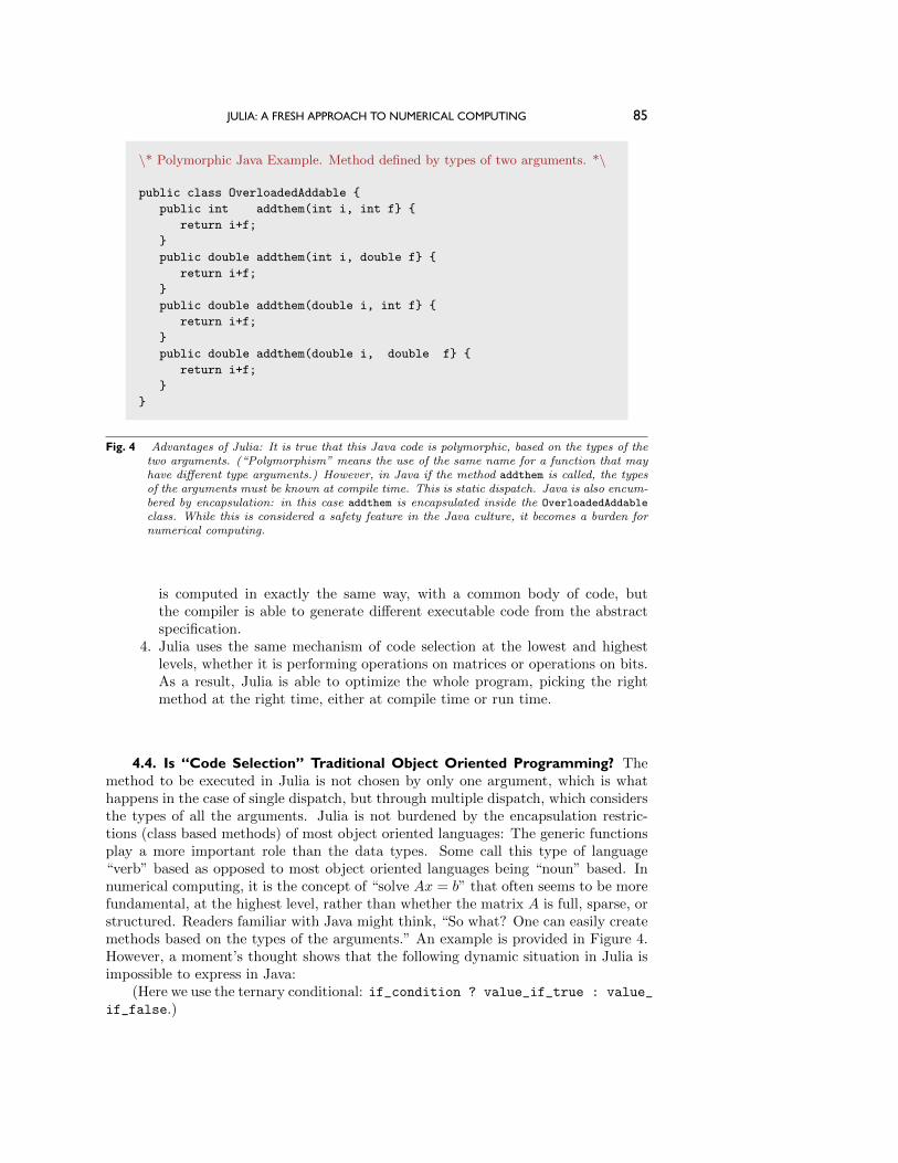
Fig. 4 Advantages of Julia: It is true that this Java code is polymorphic, based on the types of thetwo arguments. (“Polymorphism” means the use of the same name for a function that mayhave different type arguments.) However, in Java if the method addthem is called, the typesof the arguments must be known at compile time. This is static dispatch. Java is also encum-bered by encapsulation: in this case addthem is encapsulated inside the OverloadedAddable

class. While this is considered a safety feature in the Java culture, it becomes a burden fornumerical computing.

is computed in exactly the same way, with a common body of code, butthe compiler is able to generate different executable code from the abstractspecification.

4. Julia uses the same mechanism of code selection at the lowest and highestlevels, whether it is performing operations on matrices or operations on bits.As a result, Julia is able to optimize the whole program, picking the rightmethod at the right time, either at compile time or run time.

4.4. Is “Code Selection” Traditional Object Oriented Programming? Themethod to be executed in Julia is not chosen by only one argument, which is whathappens in the case of single dispatch, but through multiple dispatch, which considersthe types of all the arguments. Julia is not burdened by the encapsulation restric-tions (class based methods) of most object oriented languages: The generic functionsplay a more important role than the data types. Some call this type of language“verb” based as opposed to most object oriented languages being “noun” based. Innumerical computing, it is the concept of “solve Ax = b” that often seems to be morefundamental, at the highest level, rather than whether the matrix A is full, sparse, orstructured. Readers familiar with Java might think, “So what? One can easily createmethods based on the types of the arguments.” An example is provided in Figure 4.However, a moment’s thought shows that the following dynamic situation in Julia isimpossible to express in Java:

(Here we use the ternary conditional: if_condition ? value_if_true : value_

if_false.)


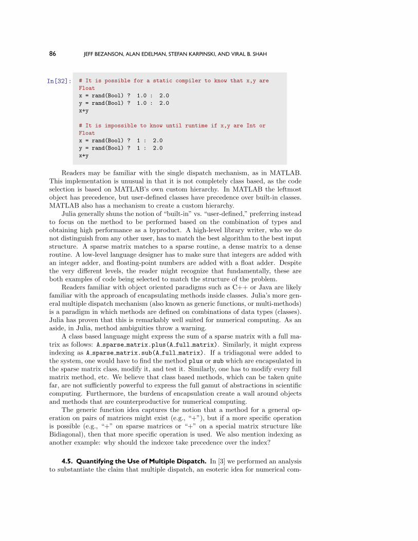
In[32]: # It is possible for a static compiler to know that x,y are

Float

x = rand(Bool) ? 1.0 : 2.0

y = rand(Bool) ? 1.0 : 2.0

x+y

# It is impossible to know until runtime if x,y are Int or

Float

x = rand(Bool) ? 1 : 2.0

y = rand(Bool) ? 1 : 2.0

x+y

Readers may be familiar with the single dispatch mechanism, as in MATLAB.This implementation is unusual in that it is not completely class based, as the codeselection is based on MATLAB’s own custom hierarchy. In MATLAB the leftmostobject has precedence, but user-defined classes have precedence over built-in classes.MATLAB also has a mechanism to create a custom hierarchy.

Julia generally shuns the notion of “built-in” vs. “user-defined,” preferring insteadto focus on the method to be performed based on the combination of types andobtaining high performance as a byproduct. A high-level library writer, who we donot distinguish from any other user, has to match the best algorithm to the best inputstructure. A sparse matrix matches to a sparse routine, a dense matrix to a denseroutine. A low-level language designer has to make sure that integers are added withan integer adder, and floating-point numbers are added with a float adder. Despitethe very different levels, the reader might recognize that fundamentally, these areboth examples of code being selected to match the structure of the problem.

Readers familiar with object oriented paradigms such as C++ or Java are likelyfamiliar with the approach of encapsulating methods inside classes. Julia’s more gen-eral multiple dispatch mechanism (also known as generic functions, or multi-methods)is a paradigm in which methods are defined on combinations of data types (classes).Julia has proven that this is remarkably well suited for numerical computing. As anaside, in Julia, method ambiguities throw a warning.

A class based language might express the sum of a sparse matrix with a full ma-trix as follows: A sparse matrix.plus(A full matrix). Similarly, it might expressindexing as A sparse matrix.sub(A full matrix). If a tridiagonal were added tothe system, one would have to find the method plus or sub which are encapsulated inthe sparse matrix class, modify it, and test it. Similarly, one has to modify every fullmatrix method, etc. We believe that class based methods, which can be taken quitefar, are not sufficiently powerful to express the full gamut of abstractions in scientificcomputing. Furthermore, the burdens of encapsulation create a wall around objectsand methods that are counterproductive for numerical computing.

The generic function idea captures the notion that a method for a general op-eration on pairs of matrices might exist (e.g., “+”), but if a more specific operationis possible (e.g., “+” on sparse matrices or “+” on a special matrix structure likeBidiagonal), then that more specific operation is used. We also mention indexing asanother example: why should the indexee take precedence over the index?

4.5. Quantifying the Use of Multiple Dispatch. In [3] we performed an analysisto substantiate the claim that multiple dispatch, an esoteric idea for numerical com-


Table 1 A comparison of Julia (1208 functions exported from the Base library) to other languageswith multiple dispatch. The “Julia operators” row describes 47 functions with special syntax(binary operators, indexing, and concatenation). Data for other systems are from [26]. Theresults indicate that Julia is using multiple dispatch far more heavily than previous systems.

Language DR CR DoS

Gwydion 1.74 18.27 2.14OpenDylan 2.51 43.84 1.23CMUCL 2.03 6.34 1.17SBCL 2.37 26.57 1.11McCLIM 2.32 15.43 1.17Vortex 2.33 63.30 1.06Whirlwind 2.07 31.65 0.71NiceC 1.36 3.46 0.33LocStack 1.50 8.92 1.02Julia 5.86 51.44 1.54Julia operators 28.13 78.06 2.01

puting from computer languages, finds its killer application in scientific computing.We wanted to answer for ourselves the question of whether there was really anythingdifferent about how Julia uses multiple dispatch.

Table 1 gives an answer in terms of dispatch ratio (DR), choice ratio (CR), anddegree of specialization (DoS). While multiple dispatch is an idea that has been cir-culating for some time, its application to numerical computing appears to have sig-nificantly favorable characteristics compared to previous applications.

To quantify how heavily a language feature is used, we use the following met-rics [26]:

1. Dispatch ratio: The average number of methods in a generic function.2. Choice ratio: For each method, the total number of methods over all generic

functions it belongs to, averaged over all methods. This is essentially the sumof the squares of the number of methods in each generic function, divided bythe total number of methods. The intent of this statistic is to give moreweight to functions with a large number of methods.

3. Degree of specialization: The average number of type-specialized argumentsper method.

Table 1 shows the mean of each metric over the entire Julia Base library, showinga high degree of multiple dispatch compared with corpora in other languages [26].Compared to most multiple dispatch systems, Julia functions tend to have a largenumber of definitions. To see why this might be so, it helps to compare resultsfrom a biased sample of common operators. These functions are the most obviouscandidates for multiple dispatch, and as a result their statistics climb dramatically.Julia is focused on numerical computing, and so is likely to have a large proportionof functions with this characteristic.

4.6. Case Study for Numerical Computing. The complexity of linear algebrasoftware has been nicely captured in the context of LAPACK and ScaLAPACK byDemmel, Dongarra et al. [7] and is reproduced verbatim here:

(1) for all linear algebra problems

(linear systems, eigenproblems, ...)

(2) for all matrix types

(general, symmetric, banded, ...)


(3) for all data types

(real, complex, single, double, higher precision)

(4) for all machine architectures

and communication topologies

(5) for all programming interfaces provide the

(6) best algorithm(s) available in terms of

performance and accuracy ("algorithms"

is plural because sometimes no single

one is always best)

In the language of computer science, code reuse is about taking advantage ofpolymorphism. In the general language of mathematics it’s about taking advantageof abstraction, or the sameness of two things. Either way, programs are efficient,powerful, and maintainable if programmers are given powerful mechanisms to reusecode.

Increasingly, the applicability of linear algebra has gone well beyond the worldof floating-point numbers. These days linear algebra is performed on high precisionnumbers, integers, elements of finite fields, and rational numbers. There will always bea special place for the BLAS and the performance it provides for floating-point num-bers. Nevertheless, linear algebra operations transcend any one data type. One mustbe able to write a general implementation and, as long as the necessary operationsare available, the code should just work [27]. That is the power of code reuse.

4.6.1. Determinant: Simple Single Dispatch. In traditional numerical comput-ing there are people with special skills known as library writers. Most users are, well,just users of libraries. In this case study, we show how anybody can dispatch a newdeterminant function based solely on the type of the argument.

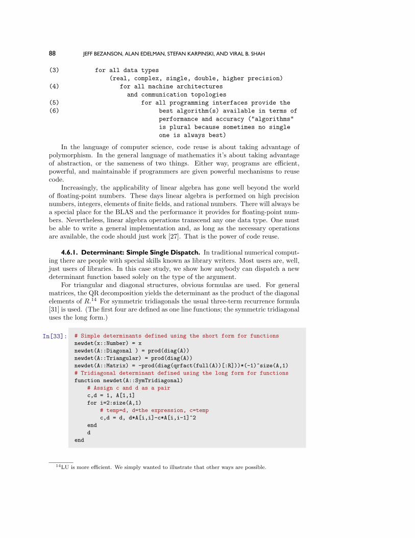
For triangular and diagonal structures, obvious formulas are used. For generalmatrices, the QR decomposition yields the determinant as the product of the diagonalelements of R.14 For symmetric tridiagonals the usual three-term recurrence formula[31] is used. (The first four are defined as one line functions; the symmetric tridiagonaluses the long form.)

In[33]: # Simple determinants defined using the short form for functions

newdet(x::Number) = x

newdet(A::Diagonal ) = prod(diag(A))

newdet(A::Triangular) = prod(diag(A))

newdet(A::Matrix) = -prod(diag(qrfact(full(A))[:R]))*(-1)^size(A,1)

# Tridiagonal determinant defined using the long form for functions

function newdet(A::SymTridiagonal)

# Assign c and d as a pair

c,d = 1, A[1,1]

for i=2:size(A,1)

# temp=d, d=the expression, c=temp

c,d = d, d*A[i,i]-c*A[i,i-1]^2

end

d

end

14LU is more efficient. We simply wanted to illustrate that other ways are possible.


We have illustrated a mechanism to select a formula at run time based on theinput type.

4.6.2. A Symmetric Arrow Matrix Type. There exist matrix structures andoperations on those matrices. In Julia, these structures exist as Julia types. Julia hasa number of predefined matrix structure types: (dense) Matrix, (compressed sparsecolumn) SparseMatrixCSC, Symmetric, Hermitian, SymTridiagonal, Bidiagonal,Tridiagonal, Diagonal, and Triangular are all examples of its matrix structures.

The operations on these matrices exist as Julia functions. Familiar examplesof operations are indexing, determinant, size, and matrix addition. Since matrixaddition takes two arguments, it may be necessary to reconcile two different typeswhen computing the sum.

In the following Julia example, we illustrate how the user can add symmetricarrow matrices to the system, and then add a specialized det method to computethe determinant of a symmetric arrow matrix efficiently. We build on the symmetricarrow type introduced in section 3.3.

In[34]: # Define a Symmetric Arrow Matrix Type

immutable SymArrow{T} <: AbstractMatrix{T}dv::Vector{T} # diagonal

ev::Vector{T} # 1st row[2:n]

end

In[35]: # Define its size

importall Base

size(A::SymArrow, dim::Integer) = size(A.dv,1)

size(A::SymArrow)= size(A,1), size(A,1)

Out[35]: size (generic function with 52 methods)

In[36]: # Index into a SymArrow

function getindex(A::SymArrow,i::Integer,j::Integer)

if i==j; return A.dv[i]

elseif i==1; return A.ev[j-1]

elseif j==1; return A.ev[i-1]

else return zero(typeof(A.dv[1]))

end

end

Out[36]: getindex (generic function with 168 methods)

In[37]: # Dense version of SymArrow

full(A::SymArrow) =[A[i,j] for i=1:size(A,1), j=1:size(A,2)]

Out[37]: full (generic function with 17 methods)

In[38]: # An example

S=SymArrow([1,2,3,4,5],[6,7,8,9])


Out[38]: 5x5 SymArrow{Int64}:1 6 7 8 9

6 2 0 0 0

7 0 3 0 0

8 0 0 4 0

9 0 0 0 5

In[39]: # det for SymArrow (external dispatch example)

function exc prod(v) # prod(v)/v[i]

[prod(v[[1:(i-1),(i+1):end]]) for i=1:size(v,1)]

end

# det for SymArrow formula

det(A::SymArrow) = prod(A.dv)-sum(A.ev.^2.*exc prod(A.dv[2:end]))

Out[39]: det (generic function with 17 methods)

The above Julia code uses the formula det(A) =∏ni=1 di −

∑ni=2 e

2i

∏2≤j 6=i≤n dj ,

valid for symmetric arrow matrices where d is the diagonal and e is the first rowstarting with the second entry.

In some numerical computing languages, a function might begin with a lot ofargument checking to pick which algorithm to use. In Julia, one creates a number ofmethods. Thus, newdet as defined by In [33] on a diagonal is one method for newdet,and newdet on a triangular matrix is a second method. In practice, one would overloaddet itself as shown in In [39] for SymArrow matrices: det on a SymArrow is a newmethod for det. (See section 4.6.1.)

We have now seen a number of examples of code selection for single dispatch, i.e.,the selection of code based on the type of a single argument. We might notice that asymmetric arrow plus a diagonal does not require operations on full dense matrices.The code below starts with the most general case, and then allows for specializationfor the symmetric arrow and diagonal sum:

In[40]: # SymArrow + Any Matrix: (Fallback: add full dense arrays )

+(A::SymArrow, B::Matrix) = full(A)+B

+(B::Matrix, A::SymArrow) = A+B # Define B+A as A+B

# SymArrow + Diagonal: (Special case: add diagonals, copy

off-diagonal)

+(A::SymArrow, B::Diagonal) = SymArrow(A.dv+B.diag,A.ev)

+(B::Diagonal, A::SymArrow) = A+B

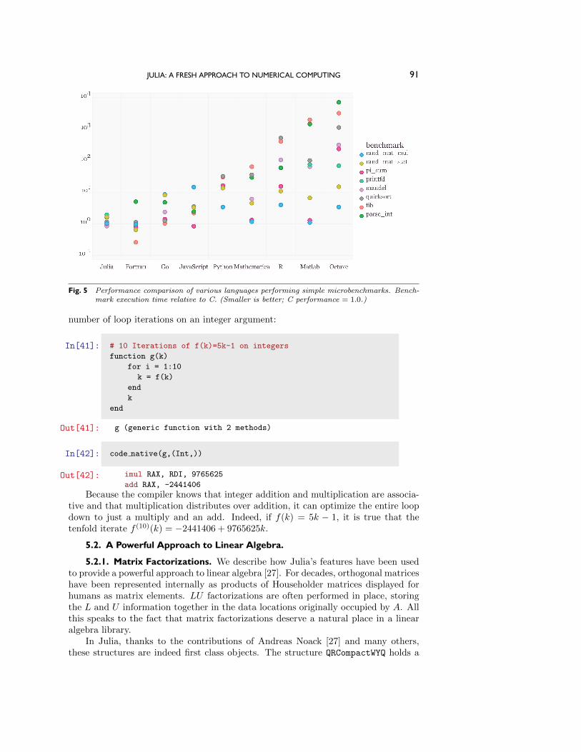
5. Leveraging Design for High Performance Libraries. Seemingly innocuousdesign choices in a language can have profound, pervasive performance implications.These are often overlooked in languages that were not designed from the beginningto be able to deliver excellent performance. See Figure 5. Other aspects of languageand library design affect the usability, composability, and power of the provided func-tionality.

5.1. Integer Arithmetic. A simple but crucial example of a performance-criticallanguage design choice is integer arithmetic. Consider what happens if we make a fixed


Fig. 5 Performance comparison of various languages performing simple microbenchmarks. Bench-mark execution time relative to C. (Smaller is better; C performance = 1.0.)

number of loop iterations on an integer argument:

In[41]: # 10 Iterations of f(k)=5k-1 on integers

function g(k)

for i = 1:10

k = f(k)

end

k

end

Out[41]: g (generic function with 2 methods)

In[42]: code native(g,(Int,))

Out[42]: imul RAX, RDI, 9765625

add RAX, -2441406

Because the compiler knows that integer addition and multiplication are associa-tive and that multiplication distributes over addition, it can optimize the entire loopdown to just a multiply and an add. Indeed, if f(k) = 5k − 1, it is true that thetenfold iterate f (10)(k) = −2441406 + 9765625k.

5.2. A Powerful Approach to Linear Algebra.

5.2.1. Matrix Factorizations. We describe how Julia’s features have been usedto provide a powerful approach to linear algebra [27]. For decades, orthogonal matriceshave been represented internally as products of Householder matrices displayed forhumans as matrix elements. LU factorizations are often performed in place, storingthe L and U information together in the data locations originally occupied by A. Allthis speaks to the fact that matrix factorizations deserve a natural place in a linearalgebra library.

In Julia, thanks to the contributions of Andreas Noack [27] and many others,these structures are indeed first class objects. The structure QRCompactWYQ holds a


compact Q and an R in memory. Similarly, an LU holds an L and a U in packed formin memory. Through the magic of multiple dispatch, we can solve linear systems,extract the pieces, and do least squares directly on these structures.

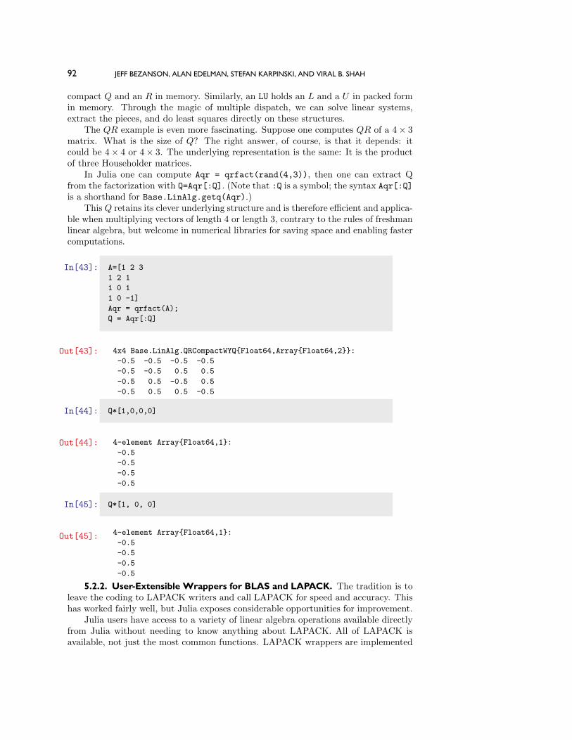
The QR example is even more fascinating. Suppose one computes QR of a 4× 3matrix. What is the size of Q? The right answer, of course, is that it depends: itcould be 4× 4 or 4× 3. The underlying representation is the same: It is the productof three Householder matrices.

In Julia one can compute Aqr = qrfact(rand(4,3)), then one can extract Qfrom the factorization with Q=Aqr[:Q]. (Note that :Q is a symbol; the syntax Aqr[:Q]

is a shorthand for Base.LinAlg.getq(Aqr).)This Q retains its clever underlying structure and is therefore efficient and applica-

ble when multiplying vectors of length 4 or length 3, contrary to the rules of freshmanlinear algebra, but welcome in numerical libraries for saving space and enabling fastercomputations.

In[43]: A=[1 2 3

1 2 1

1 0 1

1 0 -1]

Aqr = qrfact(A);

Q = Aqr[:Q]

Out[43]: 4x4 Base.LinAlg.QRCompactWYQ{Float64,Array{Float64,2}}:

-0.5 -0.5 -0.5 -0.5

-0.5 -0.5 0.5 0.5

-0.5 0.5 -0.5 0.5

-0.5 0.5 0.5 -0.5

In[44]: Q*[1,0,0,0]

Out[44]: 4-element Array{Float64,1}:

-0.5

-0.5

-0.5

-0.5

In[45]: Q*[1, 0, 0]

Out[45]: 4-element Array{Float64,1}:

-0.5

-0.5

-0.5

-0.5

5.2.2. User-Extensible Wrappers for BLAS and LAPACK. The tradition is toleave the coding to LAPACK writers and call LAPACK for speed and accuracy. Thishas worked fairly well, but Julia exposes considerable opportunities for improvement.

Julia users have access to a variety of linear algebra operations available directlyfrom Julia without needing to know anything about LAPACK. All of LAPACK isavailable, not just the most common functions. LAPACK wrappers are implemented


fully in Julia code, using ccall,15 which does not require a C compiler and can becalled directly from the interactive Julia prompt.

Consider the Cholesky factorization by calling LAPACK’s xPOTRF. It uses Julia’smetaprogramming facilities to generate four functions, corresponding to the xPOTRF

functions for Float32, Float64, Complex64, and Complex128 types. The call to theFortran functions is wrapped in ccall.

In[46]: # Generate calls to LAPACK’s Cholesky for double, single, etc.

# xPOTRF refers to POsitive definite TRiangular Factor

# LAPACK signature: SUBROUTINE DPOTRF( UPLO, N, A, LDA, INFO )

* UPLO (input) CHARACTER*1

* N (input) INTEGER

* A (input/output) DOUBLE PRECISION array, dimension (LDA,N)

* LDA (input) INTEGER

* INFO (output) INTEGER

# Generate Julia method potrf!

for (potrf, elty) in # Run through 4 element types

((:dpotrf_,:Float64),

(:spotrf_,:Float32),

(:zpotrf_,:Complex128),

(:cpotrf_,:Complex64))

# Begin function potrf!

@eval begin

function potrf!(uplo::Char, A::StridedMatrix{$elty})

lda = max(1,stride(A,2))

lda==0 && return A, 0

info = Array(Int, 1)

# Call to LAPACK:ccall(LAPACKroutine,Void,PointerTypes,JuliaVariables)

ccall(($(string(potrf)),:liblapack), Void,

(Ptr{Char}, Ptr{Int}, Ptr{$elty}, Ptr{Int}, Ptr{Int}),

&uplo, &size(A,1), A, &lda,

info)

return A, info[1]

end

end

end

chol(A::Matrix) = potrf!(’U’, copy(A))

5.3. High Performance Polynomials and Special Functions with Macros. Ju-lia has a macro system that provides custom code generation, providing performancethat is otherwise difficult to achieve. A macro is a function that runs at parse time,takes symbolic expressions in, and returns transformed expressions out, which areinserted into the code for later compilation. For example, a library developer hasimplemented an @evalpoly macro that uses Horner’s rule to evaluate polynomialsefficiently. Consider

In[47]: @evalpoly(10,3,4,5,6)

15http://docs.julialang.org/en/latest/manual/calling-c-and-fortran-code/

http://docs.julialang.org/en/latest/manual/calling-c-and-fortran-code/


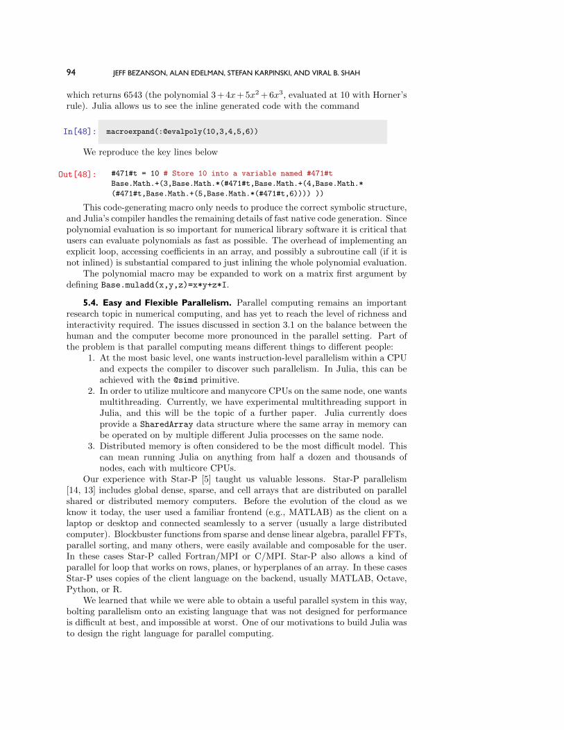
which returns 6543 (the polynomial 3 + 4x+ 5x2 + 6x3, evaluated at 10 with Horner’srule). Julia allows us to see the inline generated code with the command

In[48]: macroexpand(:@evalpoly(10,3,4,5,6))

We reproduce the key lines below

Out[48]: #471#t = 10 # Store 10 into a variable named #471#t

Base.Math.+(3,Base.Math.*(#471#t,Base.Math.+(4,Base.Math.*

(#471#t,Base.Math.+(5,Base.Math.*(#471#t,6)))) ))

This code-generating macro only needs to produce the correct symbolic structure,and Julia’s compiler handles the remaining details of fast native code generation. Sincepolynomial evaluation is so important for numerical library software it is critical thatusers can evaluate polynomials as fast as possible. The overhead of implementing anexplicit loop, accessing coefficients in an array, and possibly a subroutine call (if it isnot inlined) is substantial compared to just inlining the whole polynomial evaluation.

The polynomial macro may be expanded to work on a matrix first argument bydefining Base.muladd(x,y,z)=x*y+z*I.

5.4. Easy and Flexible Parallelism. Parallel computing remains an importantresearch topic in numerical computing, and has yet to reach the level of richness andinteractivity required. The issues discussed in section 3.1 on the balance between thehuman and the computer become more pronounced in the parallel setting. Part ofthe problem is that parallel computing means different things to different people:

1. At the most basic level, one wants instruction-level parallelism within a CPUand expects the compiler to discover such parallelism. In Julia, this can beachieved with the @simd primitive.

2. In order to utilize multicore and manycore CPUs on the same node, one wantsmultithreading. Currently, we have experimental multithreading support inJulia, and this will be the topic of a further paper. Julia currently doesprovide a SharedArray data structure where the same array in memory canbe operated on by multiple different Julia processes on the same node.

3. Distributed memory is often considered to be the most difficult model. Thiscan mean running Julia on anything from half a dozen and thousands ofnodes, each with multicore CPUs.

Our experience with Star-P [5] taught us valuable lessons. Star-P parallelism[14, 13] includes global dense, sparse, and cell arrays that are distributed on parallelshared or distributed memory computers. Before the evolution of the cloud as weknow it today, the user used a familiar frontend (e.g., MATLAB) as the client on alaptop or desktop and connected seamlessly to a server (usually a large distributedcomputer). Blockbuster functions from sparse and dense linear algebra, parallel FFTs,parallel sorting, and many others, were easily available and composable for the user.In these cases Star-P called Fortran/MPI or C/MPI. Star-P also allows a kind ofparallel for loop that works on rows, planes, or hyperplanes of an array. In these casesStar-P uses copies of the client language on the backend, usually MATLAB, Octave,Python, or R.

We learned that while we were able to obtain a useful parallel system in this way,bolting parallelism onto an existing language that was not designed for performanceis difficult at best, and impossible at worst. One of our motivations to build Julia wasto design the right language for parallel computing.


Julia provides many facilities for parallelism, which are described in detail in theJulia manual.16 Distributed memory programming in Julia is built on two primitives—remote calls that execute a function on a remote processor and remote references thatare returned by the remote processor to the caller. These primitives are implementedcompletely within Julia. On top of them, Julia provides a distributed array datastructure, a pmap implementation, and a way to parallelize independent iterations ofa loop with the @parallel macro, all of which can parallelize code in distributedmemory. These ideas are exploratory in nature, and we only discuss them here to em-phasize that well-designed programming language abstractions and primitives allowone to express and implement parallelism completely within the language.

We proceed with one example that demonstrates parallel computing at work andshows how one can impulsively grab a large number of processors and explore theirproblem space quickly.

In[49]: addprocs(1024) # define on every processor

@everywhere function stochastic(β=2,n=200)h=n^-(1/3)

x=0:h:10

N=length(x)

d=(-2/h^2 .-x) + 2sqrt(h*β)*randn(N) # diagonal

e=ones(N-1)/h^2 # subdiagonal

eigvals(SymTridiagonal(d,e))[N] # smallest negative eigenvalue

end

In[50]: using StatsBase

using PyPlot

println("Sequential version")

t = 10000

for β=[1,2,4,10,20]z = fit(Histogram, [stochastic(β) for i=1:t], -4:0.01:1).weights

plot(midpoints(-4:0.01:1), z/sum(z)/0.01)

end

16http://docs.julialang.org/en/latest/manual/parallel-computing/

http://docs.julialang.org/en/latest/manual/parallel-computing/


Suppose we wish to perform a complicated histogram in parallel. We use anexample from random matrix theory, (but it could easily have been from finance), thecomputation of the scaled largest eigenvalue in magnitude of the so-called stochastic

Airy operator: [8] d2

dx2 − x+ 12√βdW. This is the usual finite difference discretization

of d2

dx2 − x with a “noisy” diagonal.We illustrate an example of the famous Tracy–Widom law being simulated with

Monte Carlo experiments for different values of the inverse temperature parameter β.The simulation on one processor is fuzzy and unfocused, as compared to the samesimulation on 1024 processors, which is sharp and focused and runs in exactly thesame wall clock time as the sequential run.

In[51]: # Readily adding 1024 processors sharpens the Monte Carlo simulation,

# computing 1024 times as many samples in the same time

In[52]: println("@parallel version")

@everywhere t = 10000

for β=[1,2,4,10,20]z = @parallel (+) for p = 1:nprocs()

fit(Histogram, [stochastic(β) for i = 1:t], -4:0.01:1).weights

end

plot(midpoints(-4:0.01:1), z/sum(z)/0.01)

end

5.5. Performance Recap. In the early days of high-level numerical computinglanguages, the thinking was that the performance of the high-level language did notmatter so long as most of the time was spent inside the numerical libraries. Theselibraries consisted of blockbuster algorithms that would be highly tuned, makingefficient use of computer memory, cache, and low-level instructions.

What the world learned was that only a few codes spent a majority of theirtime in the blockbusters. Most codes were being hampered by interpreter overheads,stemming from processing more aspects of a program at run time than are strictlynecessary.

As we explored in section 3, one of the hindrances to completing this analysisis type information. Programming language design thus becomes an exercise in bal-ancing incentives to the programmer to provide type information and the ability ofthe computer to infer type information. Vectorization is one such incentive system.


Existing numerical computing languages would have us believe that this is the onlysystem or, even if there are others, that somehow this is the best system.

Vectorization at the software level can be elegant for some problems. There aremany matrix computation problems that look beautiful vectorized. These programsshould be vectorized. Other programs require heroics and skill to vectorize, sometimesproducing unreadable code all in the name of performance. These programs we objectto vectorizing. Still other programs cannot be vectorized very well, even with heroics.The Julia message is to vectorize when it is natural, producing nice code. Do notvectorize in the name of speed.

Some users believe that vectorization is required to make use of special hardwarecapabilities such as SIMD instructions, multithreading, GPU units, and other formsof parallelism. This is not strictly true, as compilers are increasingly able to applythese performance features to explicit loops. The Julia message remains the same:vectorize when natural, when you feel it is right.

6. Conclusion. We built Julia to meet our needs for numerical computing, andit turns out that many others wanted exactly the same thing. At the time of writ-ing, not a day goes by when we don’t learn that someone new has picked up Juliaat universities and companies around the world, in fields as diverse as engineering,mathematics, physical and social sciences, finance, biotech, and many others. Morethan just a language, Julia has become a place for programmers, physical scientists,social scientists, computational scientists, mathematicians, and others to pool theircollective knowledge in the form of online discussions and code.

Acknowledgments. Julia would not have been possible without the enthusiasmand contributions of the Julia community17 and of MIT during early years of its de-velopment. We thank Michael La Croix for his beautiful Julia display macros. We areindebted at MIT to Jeremy Kepner, Chris Hill, Saman Amarasinghe, Charles Leiser-son, Steven Johnson, and Gil Strang for their collegial support, which not only allowedfor the possibility of an academic research project to update technical computing, butmade it more fun, too.

REFERENCES

[1] E. Anderson, Z. Bai, C. Bischof, S. Blackford, J. Demmel, J. Dongarra, J. Du Croz,A. Greenbaum, S. Hammarling, A. McKenney, and D. Sorensen, LAPACK Users’Guide, 3rd ed., SIAM, Philadelphia, PA, 1999. (Cited on p. 73)

[2] J. Bezanson, Abstraction in Technical Computing, Ph.D. thesis, Massachusetts Institute ofTechnology, MA, 2015. (Cited on p. 68)

[3] J. Bezanson, J. Chen, S. Karpinski, V. B. Shah, and A. Edelman, Array operators usingmultiple dispatch, in ARRAY’14: Proceedings of ACM SIGPLAN International Workshopon Libraries, Languages, and Compilers for Array Programming, ACM, New York, 2014,pp. 56:56–56:61. (Cited on p. 86)

[4] J. Bezanson, S. Karpinski, V. B. Shah, and A. Edelman, Julia: A Fast Dynamic Languagefor Technical Computing, preprint, arXiv:1209.5145 [cs.PL], 2012. (Cited on pp. 68, 78)

[5] R. Choy and A. Edelman, Parallel MATLAB: Doing it right, Proc. IEEE, 93 (2005), pp. 331–341. (Cited on p. 94)

[6] Clang: A C Language Family Frontend for LLVM, http://clang.llvm.org/. (Cited on p. 68)[7] J. W. Demmel, J. J. Dongarra, B. N. Parlett, W. Kahan, M. Gu, D. S. Bindel,

Y. Hida, X. S. Li, O. A. Marques, E. J. Riedy, C. Vomel, J. Langou, P. Luszczek,J. Kurzak, A. Buttari, J. Langou, and S. Tomov, Prospectus for the Next LA-PACK and ScaLAPACK Libraries, Tech. report 181, LAPACK Working Note, 2007,http://www.netlib.org/lapack/lawnspdf/lawn181.pdf. (Cited on p. 87)

17https://github.com/JuliaLang/julia/graphs/contributors

https://arxiv.org/abs/1209.5145

http://clang.llvm.org/

http://www.netlib.org/lapack/lawnspdf/lawn181.pdf


[8] A. Edelman and B. Sutton, From Random Matrices to Stochastic Operators, J. Statist.Phys., 127 (2007), pp. 1121–1165. (Cited on p. 96)

[9] The GNU MPFR Library, http://www.mpfr.org/. (Cited on p. 74)[10] C. Gomez, ed., Engineering and Scientific Computing with Scilab, Birkhauser, Boston, 1999.

(Cited on p. 66)[11] G. Hoare, Technicalities: Interactive Scientific Computing #1 of 2: Pythonic Parts, http:

//graydon2.dreamwidth.org/3186.html, 2014. (Cited on p. 74)[12] R. Ihaka and R. Gentleman, R: A language for data analysis and graphics, J. Comput.

Graph. Statist., 5 (1996), pp. 299–314. (Cited on p. 66)[13] Interactive Supercomputing, Star-p user guide. http://www-math.mit.edu/∼edelman/

publications/star-p-user.pdf. (Cited on p. 94)[14] Interactive Supercomputing, Getting Started with Star-P: Taking Your First Test-Drive,

http://www-math.mit.edu/∼edelman/publications.php, 2006. (Cited on p. 94)[15] The Jupyter Project, http://jupyter.org/. (Cited on p. 67)[16] W. Kahan, How Futile Are Mindless Assessments of Roundoff in Floating-Point Computa-

tion?, http://www.cs.berkeley.edu/∼wkahan/Mindless.pdf, 2006. (Cited on p. 72)[17] M. A. Kaplan and J. D. Ullman, A scheme for the automatic inference of variable types, J.

ACM, 27 (1980), pp. 128–145, https://doi.org/10.1145/322169.322181. (Cited on p. 78)[18] C. Lattner and V. Adve, LLVM: A compilation framework for lifelong program analysis and

transformation, in Proceedings of the 2004 International Symposium on Code Generationand Optimization (CGO’04), Palo Alto, CA, 2004, ACM, New York, 2004, pp. 75–86.(Cited on p. 68)

[19] C. L. Lawson, R. J. Hanson, D. R. Kincaid, and F. T. Krogh, Basic linear alge-bra subprograms for Fortran usage, ACM Trans. Math. Softw., 5 (1979), pp. 308–323,https://doi.org/10.1145/355841.355847. (Cited on p. 73)

[20] M. Lubin and I. Dunning, Computing in Operations Research using Julia,INFORMS J. Comput., 27 (2015), pp. 238–248, https://doi.org/10.1287/ijoc.2014.0623;arXiv preprint: http://dx.doi.org/10.1287/ijoc.2014.0623. (Cited on pp. 67, 74)

[21] Mathematica, http://www.mathematica.com. (Cited on p. 66)[22] MATLAB, http://www.mathworks.com. (Cited on p. 66)[23] The MIT License, http://opensource.org/licenses/MIT. (Cited on p. 74)[24] M. Mohnen, A graph-free approach to data-flow analysis, in Compiler Construction, R. Hor-

spool, ed., Lecture Notes in Comput. Sci. 2304, Springer, Berlin, Heidelberg, 2002, pp. 185–213. (Cited on p. 78)

[25] M. Murphy, Octave: A free, high-level language for mathematics, Linux J., 1997 (1997),326884, http://dl.acm.org/citation.cfm?id=326876.326884. (Cited on p. 66)

[26] R. Muschevici, A. Potanin, E. Tempero, and J. Noble, Multiple dispatch in practice, inProceedings of the 23rd ACM SIGPLAN Conference on Object-Oriented ProgrammingSystems Languages and Applications, OOPSLA ’08, ACM, New York, 2008, pp. 563–582,https://doi.org/10.1145/1449764.1449808. (Cited on p. 87)

[27] A. Noack, Fast and Generic Linear Algebra in Julia, Tech. report, MIT, Cambridge, MA,2015. (Cited on pp. 88, 91)

[28] J. Regier, K. Pamnany, R. Giordano, R. Thomas, D. Schlegel, J. McAuliffe, and Prab-hat, Learning an Astronomical Catalog of the Visible Universe through Scalable BayesianInference, preprint, arXiv:1611.03404 [cs.DC], 2016. (Cited on p. 67)

[29] Rust, http://www.rust-lang.org/. (Cited on p. 74)[30] H. Shen, Interactive notebooks: Sharing the code, Nature Toolbox, 515 (2014), pp. 151–152,

http://www.nature.com/news/interactive-notebooks-sharing-the-code-1.16261. (Cited onp. 67)

[31] G. Strang, Introduction to Linear Algebra, Wellesley-Cambridge Press, Wellesley, MA, 2003,https://books.google.com/books?id=Gv4pCVyoUVYC. (Cited on p. 88)

[32] Swift, https://developer.apple.com/swift/. (Cited on p. 68)[33] M. Udell, K. Mohan, D. Zeng, J. Hong, S. Diamond, and S. Boyd, Convex optimiza-

tion in Julia, in SC14 Workshop on High Performance Technical Computing in DynamicLanguages, 2014; preprint, arXiv:1410.4821 [math.OC], 2014. (Cited on p. 67)

[34] S. van der Walt, S. C. Colbert, and G. Varoquaux, The NumPy Array: A Structure forEfficient Numerical Computation, CoRR, abs/1102.1523, 2011. (Cited on p. 66)

[35] H. Wickham, ggplot2, http://ggplot2.org/. (Cited on p. 71)[36] L. Wilkinson, The Grammar of Graphics (Statistics and Computing), Springer-Verlag, New

York, 2005. (Cited on p. 71)

http://www.mpfr.org/

http://graydon2.dreamwidth.org/3186.html

http://graydon2.dreamwidth.org/3186.html

http://www-math.mit.edu/~edelman/publications/star-p-user.pdf

http://www-math.mit.edu/~edelman/publications/star-p-user.pdf

http://www-math.mit.edu/~edelman/publications.php

http://jupyter.org/

http://www.cs.berkeley.edu/~wkahan/Mindless.pdf

https://doi.org/10.1145/322169.322181

https://doi.org/10.1145/355841.355847

https://doi.org/10.1287/ijoc.2014.0623

http://dx.doi.org/10.1287/ijoc.2014.0623

http://www.mathematica.com

http://www.mathworks.com

http://opensource.org/licenses/MIT

http://dl.acm.org/citation.cfm?id=326876.326884

https://doi.org/10.1145/1449764.1449808

https://arXiv.org/abs/1611.0304

http://www.rust-lang.org/

http://www.nature.com/news/interactive-notebooks-sharing-the-code-1.16261

https://books.google.com/books?id=Gv4pCVyoUVYC

https://developer.apple.com/swift/

http://arxiv.org/abs/1410.4821

http://dblp.uni-trier.de/rec/html/journals/corr/abs-1102-1523

http://ggplot2.org/

julia: a fresh approach to numerical computing · julia: a fresh approach to numerical computing 67...

Documents