Julia Minguillon , Jaume Pujol , Kenneth Zeger

Universitat Autonoma de Barcelona, Bellaterra, Spain

University of California, San Diego

ABSTRACT

In this paper we present a progressive classification scheme for a document layout recognition system (background, text andimages) using three stages. The first stage, preprocessing, extracts statistical information that may be used for backgrounddetection and removal. The second stage, a tree based classifier, uses a variable block size and a set of probabilistic rules toclassify segmented blocks. When a block cannot be classified at a given block size because contains more than one class, it issplit in four sub-blocks that are independently classified. The third stage, postprocessing, uses the label map generated in thesecond stage with a set of context rules to label unclassified blocks, trying also to solve some of the misclassification errors thatmay have been generated during the previous stage.

The progressive scheme used in the second and third stages allows the user to stop the classification process at any blocksize, depending on his requirements. Experiments show that a progressive scheme combined with a set of postprocessing rulesincreases the percentage of correctly classified blocks and reduces the number of block computations.

Keywords: progressive classification trees, wavelet packets, document analysis

1. INTRODUCTION

Image classification plays an important role in areas such as medical imaging, aerial recognition, remote sensing, and documentlayout recognition, the subject of study of this paper. Document layout recognition is an important issue for users due to thegrowth of document storage and transmission systems such as scanners and fax machines. Image coding is a good solutionto reduce both storage requirements and transmission time. Most lossy compression systems used in image coding, suchas the JPEG standard , suffer from serious problems when images containing text are coded. An adaptive coding schemeusing different coding techniques for different image contents can improve global image quality using the appropriate codingtechnique for each image region. Therefore, systems managing mixed data such as scanners, fax machines, or printers canexploit a document layout recognition system to improve both compression and image quality. OCR systems would alsotake advantage of such a system in order to detect the text areas that need to be processed, avoiding computations over areascontaining no text.

In this paper we describe a block-based progressive scheme using classification trees (CART) and a set of postprocessingrules. Our goal is to create a robust document layout recognition system that can be used as a first stage in an adaptive codingscheme. The main idea is to differentiate background from text blocks and image blocks. In an adaptive coding scheme,background blocks need not be stored, because they contain no important information, and text blocks can be coded using adifferent technique that the one used for image blocks, for example.

This paper is organized as follows. The next section, Sect. 2, describes the architecture of the document layout recognitionsystem mentioned above. In Sect. 3 we present the results of our experiments using a set of real images scanned from severalletters, magazines and newspapers including images and text in different sizes and types. Finally, the conclusions of this paperare in Sect. 4.

email: jminguillon@ccd.uab.es, jpujol@ccd.uab.es, zeger@ucsd.edu

2. SYSTEM ARCHITECTURE

The classifier we develop in this paper is a block-based classifier based on the following idea: larger blocks can be betterclassified than smaller blocks because they contain more information, reducing also the total number of blocks to be processed.If a block cannot be classified at a given size because it contains more than one class, it is labeled as mixed class, then it is splitin four sub-blocks and the classification process is repeated for each sub-block. This process stops when a small enough blocksize is reached and no mixed blocks are found.

To build a progressive classifier such as mentioned above we have divide the classification process into three stages. Thefirst stage, called preprocessing, extracts information from the image that will be used in later stages, and preparing the imageto be classified, segmenting it in blocks. The second stage is a classification process that assigns a label to each block, using aspecial label for blocks that cannot be classified at that block size. The third stage, called postprocessing, uses the label mapgenerated by the classification stage and decides to change or not some labels depending on a set of rules. Classification andpostprocessing stages are repeated dividing the block size in each iteration, until all blocks are classified (at the smallest blocksize or before). Finally, generated labels are grouped in a bottom-up fashion to yield a quad-tree decomposition as the classifierresult. We will describe each one of the stages in which our classifier is designed separately, giving appropriate directions forsystem tuning depending on user requirements.

2.1. Preprocessing stage

Usually, images are preprocessed having two goals in mind: firstly, to detect and remove image defects caused by an incorrectscanning, and secondly, to simplify classifier tasks. Therefore, many classification systems assume images to be scanned withno defects such as skewing, for example. Another use of preprocessing is background detection and removal. Nevertheless, animage may have multiple backgrounds or a variable background (another image or a business logo, for example) and thereforeglobal background detection and removal is not an easy issue. Furthermore, in a single-scan scenario such as with a fax or ahand-held scanner, it may be important to perform the entire classification process without having to read the image twice.

In order to ensure our robust system is capable of handling small user mistakes, we have trained the classifier with imagesthat have not been preprocessed. The images that form the training set suffer from small skewing, false backgrounds caused byscanning images smaller than the scanning area, and other typical user mistakes. We wanted our system to solve these kinds ofmistakes in the classification and postprocessing stages, instead of using an expensive preprocessing stage. Nevertheless, whenpreprocessing is feasible and preprocessed images are fed into the classification system, better results are obtained.

Therefore, in this stage we only segment the image in small blocks, and then the rightmost and bottommost blocks arepadded to ensure all blocks are the same size. Color images are converted to 8 bpp grayscale images, and no further prepro-cessing is applied.

2.2. Classification and regression trees

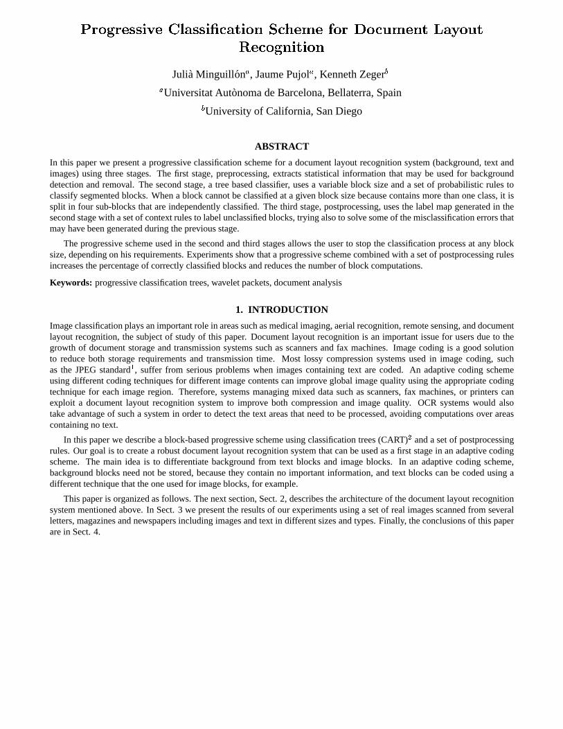
Classification and regression trees (CART) have been extensively used for data classification, such as in medical imaging,remote sensing, and character recognition. Classification trees iteratively partition the input space by applying a sequenceof questions to an input vector until a final question is answered and then a class is assigned to such vector. Fig. 1 showsan example of a classification tree. This is the tree generated for the first block size ( ), and despite its simplicity, itclassifies of blocks with accuracy. In this tree each internal node is a simple comparison , as orthogonalhyperplanes are used for space partitioning. Leaves are labeled data sets using four classes: background (B), text (T), graphicsor image (G), and mixed or undetermined (M).

Training a classification tree is a supervised process requiring a labeled training set. Each block is a -dimensional vectorrepresented by a mixture of spatial and transformed features. Vectors in the training set have been manually labeled by a

human, so the real label for each vector is also known.

A classification tree consists of a set of internal nodes and a set of leaves. Internal nodes are splitting hyperplanes thatdecide the path that an element being classified follows from the root of the tree until a leaf is reached. Each hyperplane isa partition of the -dimensional space as follows

(1)

where is a threshold which determines the side of the hyperplane an element resides.

M B G

M

T M

Figure 1. Example of a classification tree. This tree is used as the first classifier for blocks.

Leaves are labeled data sets containing a mixture of elements from different classes. A leaf is called perfect or pure whenit only contains elements from one class. The set of all leaves of a tree is represented by . In general, the optimal classifierin the sense of minimizing the Bayes risk consists of labeling a data set as

(2)

where is the cost of misclassifying an element of class as class , and is the proportion of elements of class in. This labeling strategy minimizes the misclassification error of a labeled data set.

Other authors propose the use of tree structured vector quantizers (TSVQ) for combining classification and compression ,but TSVQ suffers from a drawback when images containing a mixture of text and photos are coded. Text can often be lost in thecoded image because of insufficient codebook resolution. Furthermore, TSVQ is more expensive than CART due to the costof computing the closest codeword instead of using a splitting hyperplane (which can be a simple comparison). Therefore, wechose CART because of its simplicity and because it yields information about the internal structure of the data being classified,through an inspection of the splitting hyperplanes that form the final classification tree.

2.2.1. Classifier performance

Classifier performance is typically measured by the percentage of correctly classified blocks ( , where is thepercentage of misclassified blocks), although the Bayes risk ( ) would be a more realistic measure, because it includes in itsdefinition the misclassification cost matrix used during the training process (see Sect. 2.2.4). The Bayes risk of a tree isdefined by

and (3)

Here is the number of classes, represents the class assigned by a tree to an element , and is the true classof such element.

2.2.2. Classification features

In , a model is used with only two features, although these features include image-dependent parameters and other hiddenparameters. In contrast, we use a different tree for each stage. All trees are built using the same set of features, which consists ofa mixture of spatial features and some energy and entropy related coefficients computed after an S-Transform wavelet packetis applied to each block to be classified. This is not the case for the last stage ( ), where a DCT replaces the S-Transform.

From each block we extract a total of twenty-four spatial features including basic statistical descriptors (range, mean,median, variance, etc), fractal dimensionality, , and block histogram shape, among others. Although this set may seem com-putationally very expensive, it is not really a drawback. For example, the tree computed for the first classification stage usesonly two spatial features, so there is no need to compute the rest. An important issue in block-based image classification is thedetermination of good classification features, so we decided to compute a large set of spatial features and then select the best

ones through internal tree structure inspection. As expected, each block size needed a different set of spatial features, althoughall trees shared a common subset, showing the importance of some spatial features in image classification for document layoutrecognition systems.

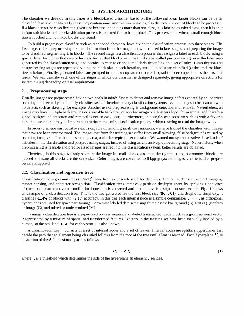
Wavelet transforms and wavelet packets have been used in image segmentation successfully. We chose the S-Transformbecause of its reordering properties, that allow us to save computations from a classification stage and reuse them in the next,using the wavelet packet decomposition showed in Fig. 2. We use two levels of decomposition but we do not apply the secondlevel in the LL quadrant, and we do not compute any energy or entropy coefficients in the LL quadrants of the second leveldecomposition. The S-Transform is interesting because it allows us to compute an approximation of the first derivative in bothdirections, using only integer operations.

Figure 2. Wavelet packet decomposition.

Once the S-Transform has been applied to a block, we compute some energy and entropy related coefficients using thetransformed block histogram. The main idea is to detect high energy coefficients in text blocks, caused by text intrinsiccharacteristics, using the entropy as an indicator of histogram shape.

If a DCT based coding scheme such as JPEG follows the classification process, it is very interesting to replace the S-Transform wavelet packet by a DCT, in order to avoid unnecessary computations. Despite its simplicity, the DCT hasbeen successfully used in other block-based classification schemes . In this case, after the DCT has been applied, we computean energy coefficient defined as

(4)

where is the subset of coefficients with higher text discrimination power .

2.2.3. Tree design

We use four trees, one tree for each block size, instead of a unique tree, in order to exploit different image characteristics ateach different block size. Furthermore, each tree uses a different set of spatial features, showing intrinsic differences betweendifferent block sizes. For example, class probabilities are different at each level, in particular the mixed class. There areof blocks labeled as mixed in the first classification stage, and this percentage decreases to for the third classificationstage, and is zero for the last. The ratio between background and non-background blocks also increases as block size is reduced,so the use of different trees and postprocessing rules at each stage allows us to extract the most important classification featuresbetter.

We start with an initial block size of and the classification process is halted at a block size of . Our training setconsists of images scanned at 150 dpi, and our experiments show that using a larger block size ( or even )for the first classification stage is almost useless, because only a few blocks are classified. Therefore, if images were scannedat 300 dpi, it would be interesting to use a first classification stage with a larger block size, such as , for example.We stop the classification process at a block size of because we assume that a coding stage follows the classifier, but alsobecause at such a small block size it is difficult to classify well, even for a human. Normal size text does not fit in a blockat 150 dpi, and text and graphics may easily confuse the classifier.

2.2.4. Training parameters

Some important parameters remain hidden during the training and pruning stages of a classification tree. These parametersdetermine the growing and pruning algorithms behavior.

Tree creation process has two stages, growing and pruning. First, a tree is grown using the training set, until a perfect(also called pure) tree is obtained, that is, all its leaves are data sets with elements in one class only. Such a tree yields a zeromisclassification error for the training set, but almost certainly overfits the corpus and test sets. Therefore, this tree needs tobe pruned back using the corpus set to ensure a good tree that does not suffer from underfitting or overfitting. Pruning is doneusing the BFOS algorithm , which prunes to a subtree with a maximum misclassification error/number of leaves ratio.

During the growing process, only orthogonal hyperplanes are used. Although this may be inefficient for splitting data setswith internal linear dependences, it simplifies the tree structure and allows the user to do a further inspection of which featuresare important for classification. Moreover, internal nodes represent simple decisions that can be efficiently coded, becauseEq. (1) is reduced to a single comparison. To compute a splitting hyperplane for a given data set, the variable that yields themaximum decrease in tree impurity (using entropy as goodness of split measure) is chosen .

During pruning, when a subset is pruned back and is replaced by a data set (a leaf), it is labeled according to the label thatminimizes the misclassification error computed during the training stage, as shown in Eq. (2). Then, a threshold conditionon the misclassification error computed for the labeled data set is used to relabel it as mixed class when its misclassificationerror exceeds some value. We have used a fixed threshold for all four sets, but it could be set to larger values forsmaller block sizes. We tested several values for and the best results were obtained using or .Therefore, pruned trees may be further simplified pruning back those subtrees that have all their leaves labeled with the sameclass (concretely, mixed class). This might generate very small pruned subtrees, so we still need another constraint to ensurewe do not generate pruned trees that do not have enough labeled data sets covering all possible classes (including mixed classor not).

The misclassification cost matrix used in our experiments is shown in Tab. 1. We used different misclassification costsfor different classes because we assume the text class (T) is more important than the image class (G), in order to preserve moretext from misclassification. For example, in case of misclassification it is better to consider text as image than to consider it asbackground. Mixed class (M) has the lowest misclassification class because it is better to delay classification than to make amistake. Similar matrices are used in other papers in literature .

B T G M

B 0 2 1.5 1

T 2 0 1.5 1

G 2 1.5 0 1

M 1.5 1 1 0

Table 1. Misclassification cost matrix.

2.3. Postprocessing rules

After each classification stage, a label map is generated as the classifier result. But even using the mixed class for uncertainblocks, some elements may have been misclassified. Then, a set of postprocessing rules is applied to each label to reduce thispossibility. This can be done in two different ways: changing a label to mixed class to avoid possible classifier mistakes, orchanging it to another class than mixed to solve classifier uncertainty. Therefore, we could classify rules as passive, whenthey only delay classification, or active, when they introduce new labels. In order to reduce misclassification errors, the twofirst classification stages use only passive rules, and a mixture of passive and active rules is used in the last two stages. Thelast classification stage has to resolve all possible unclassified blocks from previous stages, but this can be done by combiningpassive and active rules. In such case, passive rules are always applied before active rules trying to minimize the number ofclassification mistakes.

The strategy mentioned above is a top-down approach, that is, it starts at the largest block size and repeats until the smallestblock size is reached, increasing the size of the label map. Then, when an image has been completely classified, a bottom-upapproach is performed to generate a quad-tree decomposition of the label map, grouping similar labels regardless of background.

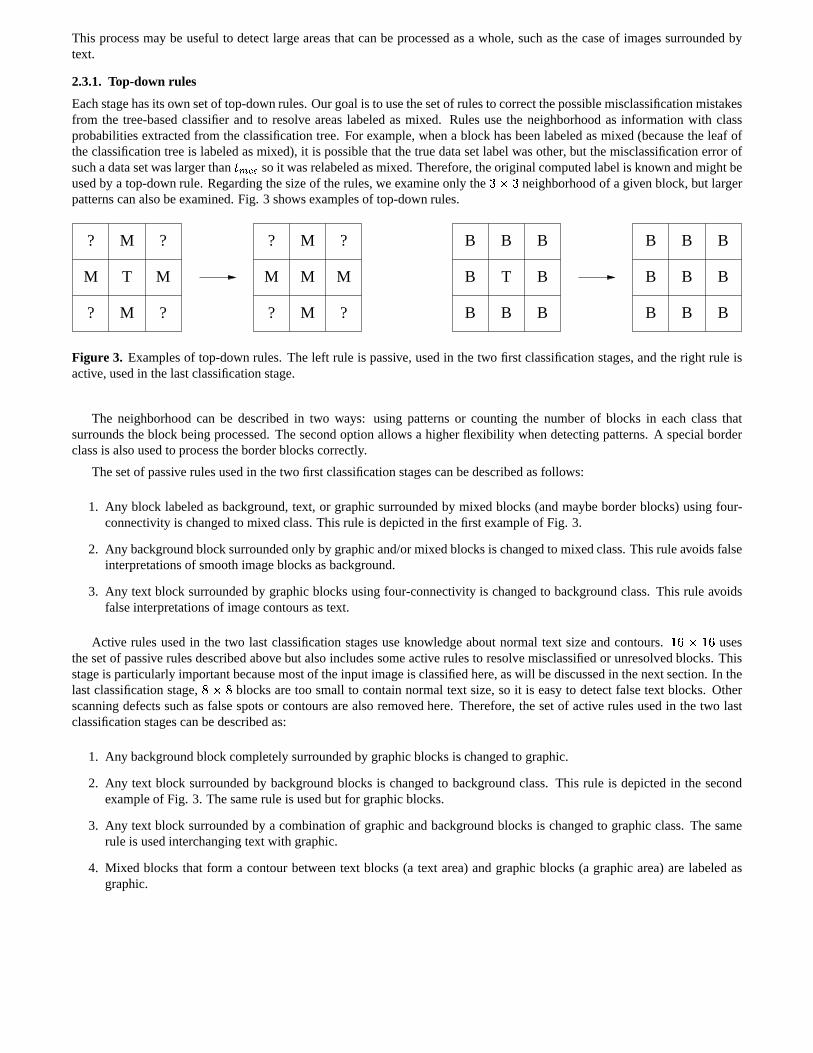
This process may be useful to detect large areas that can be processed as a whole, such as the case of images surrounded bytext.

2.3.1. Top-down rules

Each stage has its own set of top-down rules. Our goal is to use the set of rules to correct the possible misclassification mistakesfrom the tree-based classifier and to resolve areas labeled as mixed. Rules use the neighborhood as information with classprobabilities extracted from the classification tree. For example, when a block has been labeled as mixed (because the leaf ofthe classification tree is labeled as mixed), it is possible that the true data set label was other, but the misclassification error ofsuch a data set was larger than so it was relabeled as mixed. Therefore, the original computed label is known and might beused by a top-down rule. Regarding the size of the rules, we examine only the neighborhood of a given block, but largerpatterns can also be examined. Fig. 3 shows examples of top-down rules.

?

M

? M ?

?

M

? M ?

B B

B B

B

B B B

B B

B B

B

B B B

M ?

M T

M ?

M M T B

Figure 3. Examples of top-down rules. The left rule is passive, used in the two first classification stages, and the right rule isactive, used in the last classification stage.

The neighborhood can be described in two ways: using patterns or counting the number of blocks in each class thatsurrounds the block being processed. The second option allows a higher flexibility when detecting patterns. A special borderclass is also used to process the border blocks correctly.

The set of passive rules used in the two first classification stages can be described as follows:

1. Any block labeled as background, text, or graphic surrounded by mixed blocks (and maybe border blocks) using four-connectivity is changed to mixed class. This rule is depicted in the first example of Fig. 3.

2. Any background block surrounded only by graphic and/or mixed blocks is changed to mixed class. This rule avoids falseinterpretations of smooth image blocks as background.

3. Any text block surrounded by graphic blocks using four-connectivity is changed to background class. This rule avoidsfalse interpretations of image contours as text.

Active rules used in the two last classification stages use knowledge about normal text size and contours. usesthe set of passive rules described above but also includes some active rules to resolve misclassified or unresolved blocks. Thisstage is particularly important because most of the input image is classified here, as will be discussed in the next section. In thelast classification stage, blocks are too small to contain normal text size, so it is easy to detect false text blocks. Otherscanning defects such as false spots or contours are also removed here. Therefore, the set of active rules used in the two lastclassification stages can be described as:

1. Any background block completely surrounded by graphic blocks is changed to graphic.

2. Any text block surrounded by background blocks is changed to background class. This rule is depicted in the secondexample of Fig. 3. The same rule is used but for graphic blocks.

3. Any text block surrounded by a combination of graphic and background blocks is changed to graphic class. The samerule is used interchanging text with graphic.

4. Mixed blocks that form a contour between text blocks (a text area) and graphic blocks (a graphic area) are labeled asgraphic.

5. Finally, blocks that remain unclassified in the last stage ( ) are labeled using the original label computed during thetraining stage, as shown in Eq. (2).

This set of rules ensures classification of all remaining unclassified blocks, thus minimizing the number of misclassifiedblocks. Nevertheless, it is virtually impossible to achieve a performance of of correctly classified blocks because a fewmistakes happen in the last postprocessing stage. Usually, the most common mistake is the misclassification of some parts oftext of large size or special font text as graphic. This could be only solved applying very high level rules involving informationabout what text size and/or font is considered text or graphic, which is beyond of the scope of this paper.

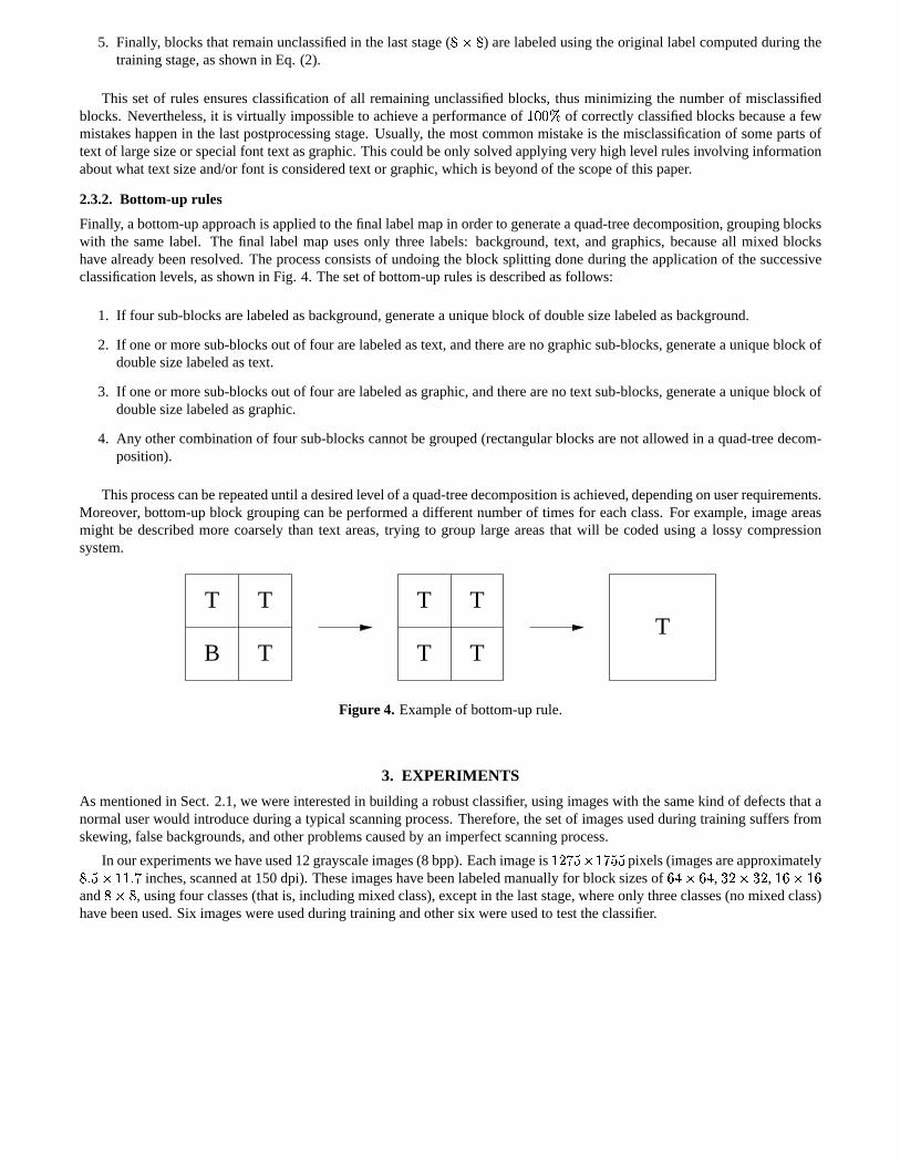
2.3.2. Bottom-up rules

Finally, a bottom-up approach is applied to the final label map in order to generate a quad-tree decomposition, grouping blockswith the same label. The final label map uses only three labels: background, text, and graphics, because all mixed blockshave already been resolved. The process consists of undoing the block splitting done during the application of the successiveclassification levels, as shown in Fig. 4. The set of bottom-up rules is described as follows:

1. If four sub-blocks are labeled as background, generate a unique block of double size labeled as background.

2. If one or more sub-blocks out of four are labeled as text, and there are no graphic sub-blocks, generate a unique block ofdouble size labeled as text.

3. If one or more sub-blocks out of four are labeled as graphic, and there are no text sub-blocks, generate a unique block ofdouble size labeled as graphic.

4. Any other combination of four sub-blocks cannot be grouped (rectangular blocks are not allowed in a quad-tree decom-position).

This process can be repeated until a desired level of a quad-tree decomposition is achieved, depending on user requirements.Moreover, bottom-up block grouping can be performed a different number of times for each class. For example, image areasmight be described more coarsely than text areas, trying to group large areas that will be coded using a lossy compressionsystem.

TTT

T T

T T

TB

Figure 4. Example of bottom-up rule.

3. EXPERIMENTS

As mentioned in Sect. 2.1, we were interested in building a robust classifier, using images with the same kind of defects that anormal user would introduce during a typical scanning process. Therefore, the set of images used during training suffers fromskewing, false backgrounds, and other problems caused by an imperfect scanning process.

In our experiments we have used 12 grayscale images (8 bpp). Each image is pixels (images are approximatelyinches, scanned at 150 dpi). These images have been labeled manually for block sizes of , ,

and , using four classes (that is, including mixed class), except in the last stage, where only three classes (no mixed class)have been used. Six images were used during training and other six were used to test the classifier.

Block minimum average maximum

size length length length

Progressive classification scheme

11 6 2 2.76696 4

27 14 2 4.16826 6

21 11 3 3.71954 6

[a,b] 35 18 2 4.73452 8

Non-progressive classification scheme

[*] 1441 721 3 8.55861 38

Table 2. Tree sizes for progressive and non-progressive classification schemes.

3.1. Tree statistics

Five trees were grown, one for each block size using information from previous levels such as the kind of blocks left unclassifiedin the previous stage, and another tree that is a classifier, marked with an asterisk in Tab. 2. Our goal is to compare theperformance of the progressive classification scheme and a classical block-based classifier, comparing both tree classificationcost and accuracy.

It can be seen from Tab. 2 that the trees that form part of the progressive classifier are small when compared to the non-progressive tree. It is possible to reduce the size of the non-progressive tree, but this imposes an increase in misclassificationerror.

3.2. System performance with no postprocessing

Tab. 3 shows the progressive classification results when no postprocessing stage is applied after each classification stage.stands for the percentage of correctly classified blocks, and is the Bayes risk as defined by Eq. (3). Notice that this cannotbe considered a valid classifier because the last stage ( [a] as shown in Tab. 3) does not classify all remaining blocks fromprevious stages. Nevertheless, we will use this tree instead of the tree using only three classes ( [b]) because it yields ahigher percentage of correctly classified blocks as a starting point to apply the set of postprocessing rules. We remark that afterthe last classification tree ( ) is applied, decreases slightly. Other experiments using blocks display the samedrawback, pointing out that this block size may not be a good choice.

Block Processed Classified Classified

size blocks blocks (stage) blocks (total)

Progressive classification scheme

3360 0.559077

7856 0.425833

21052 0.189441

[a] 27892 0.148996

[b] 27892 0.110990

Non-progressive classification scheme

[*] 211200 0.136849

Table 3. Classifier results with no postprocessing stage.

Another important result we can infer from Tabs. 2 and 3 is that although it is possible to build a single tree for imageclassification using a unique block size of , this tree yields worse results in both cost and accuracy, particularly Bayes risk,which we consider more important. Similar results for non-progressive classifiers can be found in .

If we use the tree with only three classes ( [b]), the number of blocks processed is the sum of the blocks processedin each stage, yielding a total of 60160 blocks, instead of 211200 blocks that need the non-progressive classifier ( [*]),that is, approximately only of blocks. The progressive classifier needs a total of 429238 comparisons (each visit of aninternal node is a comparison), while the non-progressive classifier needs a total of 1807578 comparisons, that is, only aof comparisons are needed. Furthermore, the trees used in the progressive classifier use only a few classification features each,while the non-progressive tree uses almost the whole set of spatial features, increasing classification process cost.

3.3. System performance with postprocessing

Tab. 4 shows the results of the progressive classification scheme after the set of postprocessing rules has been applied after eachclassification stage. In this case all remaining blocks are classified in the last stage, because the last set of rules used ensuresthis fact. It can be seen that the two first stages ( and ) only delay classification, decreasing the percentage ofclassified blocks and increasing the percentage of correctly classified blocks. On the other hand, the third and fourth stagesresolve all blocks that remain unclassified and remove most of the misclassification mistakes from previous stages. Notice thatthe third stage combined with a set of postprocessing rules significantly improves classifier results, classifying more and betterthan the previous cases with no postprocessing. On the contrary, the fourth stage increases misclassification error with respectto the third one, although it still decreases the Bayes risk.

Block Processed Classified Classified

size blocks blocks (stage) blocks (total)

3360 0.562946

7968 0.429811

21756 0.177547

[a] 25832 0.103203

Table 4. Classifier results with postprocessing stage.

Regarding the robustness of the classifier, it is shown in Tab. 5. It can be seen that most images are classified with apercentage of correctly classified blocks within a narrow set of values around the system average performance ( ). In itis stated that the percentage of correctly classified blocks is around or even sometimes , but this figure decreasesto for certain images. They do not provide classification results before postprocessing, so the importance of such astage cannot be easily determined. If we feed our classifier with preprocessed images with no false backgrounds, we achieve apercentage of correctly classified blocks up to a .

Image 1 2 3 4 5 6

Table 5. Classifier results variability.

An example is shown in Fig. 5. The first image shows the original image as it was scanned from a letter, with no preprocess-ing. It can be seen that this image suffers from a false background caused by an incorrect scanning process, and other problemslike noise due to letter quality paper and folds. The second image shows the output label map with no postprocessing. There area few blocks that remain unclassified, mostly caused by image noise and area contours. Notice the three horizontal lines causedby folds and false background, for example. Finally, the third image shows the same label map once the set of postprocessingrules described in Sect. 2.3 has been applied. It can be seen that all noise spots have been removed and a high percentage ofmisclassified blocks have been corrected. Nevertheless, a few mistakes can still be found in large or special font text areas, suchas business logos. Lines caused by false backgrounds would not appear if a better scanning process was performed.

4. CONCLUSIONS

In this paper we have presented a robust system for document layout recognition based on classification and regression treesand a set of postprocessing rules.

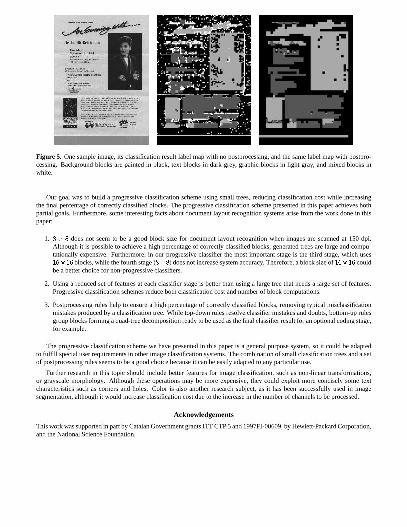
Figure 5. One sample image, its classification result label map with no postprocessing, and the same label map with postpro-cessing. Background blocks are painted in black, text blocks in dark grey, graphic blocks in light gray, and mixed blocks inwhite.

Our goal was to build a progressive classification scheme using small trees, reducing classification cost while increasingthe final percentage of correctly classified blocks. The progressive classification scheme presented in this paper achieves bothpartial goals. Furthermore, some interesting facts about document layout recognition systems arise from the work done in thispaper:

1. does not seem to be a good block size for document layout recognition when images are scanned at 150 dpi.Although it is possible to achieve a high percentage of correctly classified blocks, generated trees are large and compu-tationally expensive. Furthermore, in our progressive classifier the most important stage is the third stage, which uses

blocks, while the fourth stage ( ) does not increase system accuracy. Therefore, a block size of couldbe a better choice for non-progressive classifiers.

2. Using a reduced set of features at each classifier stage is better than using a large tree that needs a large set of features.Progressive classification schemes reduce both classification cost and number of block computations.

3. Postprocessing rules help to ensure a high percentage of correctly classified blocks, removing typical misclassificationmistakes produced by a classification tree. While top-down rules resolve classifier mistakes and doubts, bottom-up rulesgroup blocks forming a quad-tree decomposition ready to be used as the final classifier result for an optional coding stage,for example.

The progressive classification scheme we have presented in this paper is a general purpose system, so it could be adaptedto fulfill special user requirements in other image classification systems. The combination of small classification trees and a setof postprocessing rules seems to be a good choice because it can be easily adapted to any particular use.

Further research in this topic should include better features for image classification, such as non-linear transformations,or grayscale morphology. Although these operations may be more expensive, they could exploit more concisely some textcharacteristics such as corners and holes. Color is also another research subject, as it has been successfully used in imagesegmentation, although it would increase classification cost due to the increase in the number of channels to be processed.

Acknowledgements

This work was supported in part by Catalan Government grants ITT CTP 5 and 1997FI-00609, by Hewlett-Packard Corporation,and the National Science Foundation.

REFERENCES

1. G. K. Wallace, “The JPEG still picture compression standard,” Communications of the ACM ACM-34, pp. 30–44, Apr.1991.

2. L. Breiman, J. H. Friedman, R. A. Olshen, and C. J. Stone, Classification and Regression Trees, Wadsworth InternationalGroup, 1984.

3. K. O. Perlmutter, N. Chaddha, J. B. Buckheit, R. M. Gray, and R. A. Olshen, “Text segmentation in mixed-mode imagesusing classification trees and transform tree-structured vector quantization,” in Proceedings of the IEEE InternationalConference on Acoustics, Speech and Signal Processing, vol. 4, pp. 2231–2234, 1996.

4. K. O. Perlmutter, S. M. Perlmutter, R. M. Gray, R. A. Olshen, and K. L. Oehler, “Bayer risk weighted vector quantiza-tion with posterior estimation for image compression and classification,” IEEE Transactions on Image Processing IP-5,pp. 347–360, Feb. 1996.

5. J. Li and R. M. Gray, “Text and picture segmentation by the distribution analysis of wavelet coefficients,” in Proceedingsof the IEEE International Conference on Image Processing, 1998.

6. J. Li and R. M. Gray, “Context based multiscale classification of images,” in Proceedings of the IEEE InternationalConference on Image Processing, 1998.

7. A. Said and W. A. Pearlman, “An image multiresolution representation for lossless and lossy compression,” IEEE Trans-actions on Image Processing IP-5, pp. 1303–1310, Sept. 1996.

8. N. Chaddha, R. Sharma, A. Agrawal, and A. Gupta, “Text segmentation in mixed-mode images,” in Proceedings of the28th Asilomar Conference on Signals, Systems and Computers, vol. 2, pp. 1356–1361, 1995.

9. B. B. Chaudhuri and N. Sarkar, “Texture segmentation using fractal dimension,” IEEE Transactions on Pattern Analysisand Machine Intelligence PAMI-17, pp. 72–77, Jan. 1995.

10. A. Laine and J. Fan, “Texture classification by wavelet packet signatures,” IEEE Transactions on Pattern Analysis andMachine Intelligence PAMI-15, pp. 1186–1191, Nov. 1993.

11. N. Chaddha and A. Gupta, “Text segmentation using linear transforms,” in Proceedings of the 29th Asilomar Conferenceon Signals, Systems and Computers, vol. 2, pp. 1447–1451, 1996.

12. P. A. Chou, T. Lookabaugh, and R. M. Gray, “Optimal pruning with applications to tree-structured source coding andmodeling,” IEEE Transactions on Information Theory IT-35, pp. 299–315, Mar. 1989.