Using genetic algorithms to solve complex problems

Julius van der Werf

School of Rural Science and AgricultureUniversity of New England

Armidale, Australia

Complex Problems

• Multi-dimensional• Multi-objective• Multiple local optima• Flat surfaces• Non-differentiable• Variables are highly interactive• Messy

complex (animal) production problems

• Optimal resource allocation– Feeding strategies– Logistics of supply

– Total Resource Management: TRM

complex animal breeding problems

• Breeding program design– Mate selection– Development of synthetics / genetic resources

TGRM• Breeding objectives

– Non-linear profit space– Selection index weights (incl. QTL)

• Modeling – multiple QTL models– Growth models – Haplotype configuration

Solving complex problems

• Non-random numerical techniques(deterministic search algorithms)

– Linear programming– Dynamic Programming– Optimal Control Theory– Simplex algorithm

tedious

Solving complex problems

• All deterministic search algorithms

– Need to break the ‘curse of multidimensionality’

• Exhaustive (finite) search algorithms

– Job increases exponentially with problem size

Random search or stochastic algorithms

• Efficient

• Optimal solution not guaranteed – But……..

Perform better than other algorithms in complex problems à Real Time solutions

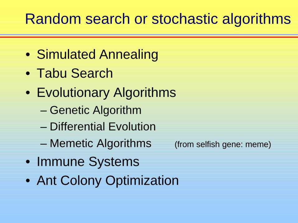
Random search or stochastic algorithms

• Simulated Annealing• Tabu Search• Evolutionary Algorithms

– Genetic Algorithm– Differential Evolution– Memetic Algorithms (from selfish gene: meme)

• Immune Systems• Ant Colony Optimization

Genetic Algorithms

• GA = “Get away with Algebra”• 30 years old

• Fitness = f(x) – x = vector with parameters

– Repeated cycles of mutationrecombinationselectionmating of parents

The Theory of Evolution

• Fitness selection• Mutation

– To create variation– Need just enough, but limited– Can it work by itself?

• The value of sex

• Recombination helps• Selection…………………….etc

As geneticists we know how powerful the concept is!

Genetic Algorithm

Recombination

11 3 0 21 5 3 19 0 21 41

49Mutation

11 4 3 0 1 3 11 26 26 0

1 2 3 4 5 6 7 8 9 10Female No. (= 'locus')

'Allele' = male allocated for breeding

• Each individual is a ‘genotype’ = possible solution

• Each genotype leads to a certain outcome (phenotype)

‘locus’

‘chr

omos

ome’

Evolutionary algorithms

• Genetic Algorithm – 70-ties

• Differential Evolution

– Price and Storn, 1997: “Dr. Dobbs Journal”

– Simple and powerful – (19 lines of C++ code)

Recombination

11 3 0 21 5 3 19 0 21 41

49Mutation

11 4 3 0 1 3 11 26 26 0

1 2 3 4 5 6 7 8 9 10

Female No. (= 'locus')

'Allele' = male allocated for breeding

Differential Evolution• Propagation is through haploids with only some sex

– Each candidate is replaced by the best of• itself • mix of itself and a competitor

• Mutation– It perturbates specific variance for each variable!

i.e. not a ‘standard random noise’ around each variable

• Recombination– For each allele change the proportions in the mix– Complementary means of creating viable vectors

• Select highest function value

The DE Algorithm

Sample base populationFor generation = 1 to maxgens

Next generation

The DE Algorithm

Sample base populationFor generation = 1 to maxgens

For individual = 1 to N_individualsDraw a challenger (from 3 pop’n members)

Compare fitness of challenger and individualReplace individual if challenger wins

Next individualNext generation

The DE Algorithm

Sample base populationFor generation = 1 to maxgens

For individual = 1 to N_individualsDraw a challenger (from 3 pop’n members)For j = 1 to N_loci

Draw allele from challenger or individualNext LocusCompare fitness of challenger and individualReplace individual if challenger wins

Next individualNext generation

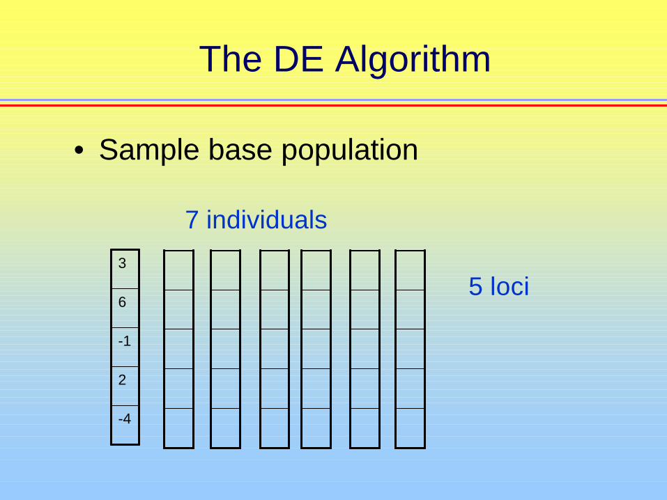
The DE Algorithm

-4

2

-1

6

3

• Sample base population

5 loci

7 individuals

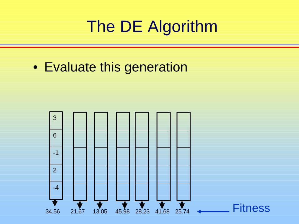
The DE Algorithm

-4

2

-1

6

3

• Evaluate this generation

Fitness34.56 21.67 45.9813.05 28.23 41.68 25.74

The DE Algorithm

-4

2

-1

6

3

• Next generation: Each individual is challenged

34.56

Xi = targetCompetes with

XT = trial,

XT = XC + F.(XA-XB)

Replace Xi with XT

If higher fitness

X1……….. XA XBXC

The DE Algorithm

-4

2

-1

6

3

34.56

Xi = target Competes with XT = XC + F.(XA-XB)

Xi XA XBXC

MutatorF= 0.4 ~ 1.2

-= + F

Xi(i) à XT(i)

If rnd > CR

Xi(i) à Xi(i)

If rnd<CRCrossoverSample alleles from target as well

as competitor CR ~ 0.8

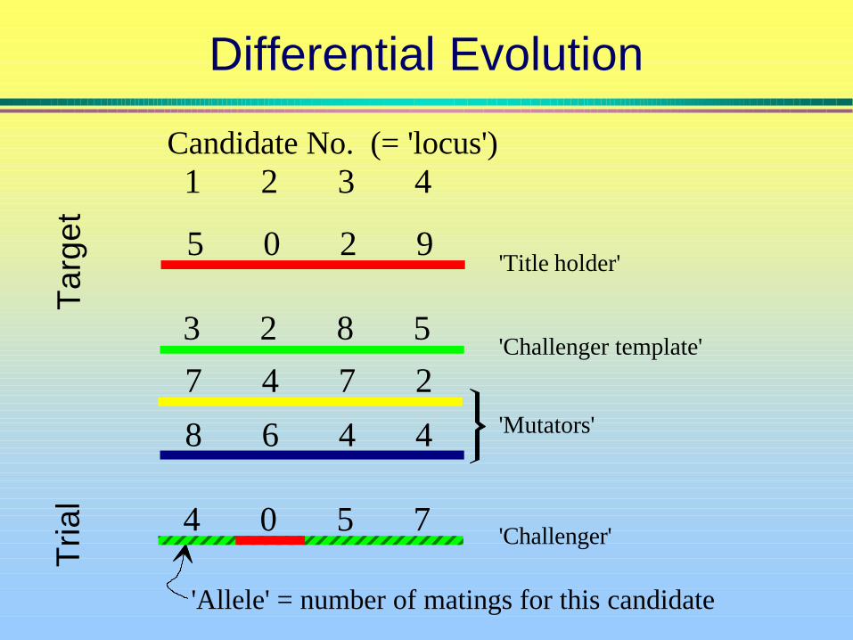
Differential Evolution

Candidate No. (= 'locus')

'Allele' = number of matings for this candidate

1 2 3 4

7 4 7 2

5 0 2 9

3 2 8 5

8 6 4 4

4 0 5 7

'Title holder'

'Challenger template'

'Mutators'

'Challenger'

Targ

etTr

ial

ExampleMax of f(x1,x2) = 0.2*x1

2 +1.45*x1

+0.035*(-0.2*x24 +3.45*x2

3 -5*x22+50*x2 +3)

Generation 0

Indiv 1Indiv 2Indiv 3Indiv 4Indiv 5Indiv 6Indiv 7Indiv 8Indiv 9Indiv 10

x1 x2 f(x1,x2)2.055 0.334 2.8100.795 -2.104 -4.5896.220 2.747 6.978-4.860 2.607 -6.4763.145 2.090 6.550-4.546 4.112 0.0113.626 2.905 8.8012.046 4.620 15.3003.714 -4.438 -21.7474.496 3.058 9.136

Example

Next generation: each individual (target) is challenged (trial), and replaced if trial > target

x1 x2 f(x1,x2)2.055 0.334 2.8100.795 4.250 12.3926.220 2.747 6.978-4.860 2.607 -6.4763.145 2.090 6.550-4.546 4.112 0.0113.626 2.905 8.8012.046 4.620 15.3003.714 3.775 11.9194.496 3.058 9.136

Generation 1x1 x2 f(x1,x2)

2.055 0.334 2.8100.795 -2.104 -4.5896.220 2.747 6.978-4.860 2.607 -6.4763.145 2.090 6.550-4.546 4.112 0.0113.626 2.905 8.8012.046 4.620 15.3003.714 -4.438 -21.7474.496 3.058 9.136

Generation 0

Example

x1 x2 f(x1,x2)3.359 12.495 62.1953.049 12.541 62.1076.892 12.407 60.1185.354 12.491 61.6145.216 12.358 61.7564.586 12.264 62.0693.534 12.237 62.2423.531 12.047 62.0944.587 12.168 62.0223.818 12.347 62.256

x1 x2 f(x1,x2)5.356 12.125 61.5754.897 12.541 61.8500.491 12.783 59.8580.491 12.123 60.2087.790 12.962 57.9142.973 9.680 51.256-5.128 7.638 20.550-0.100 12.314 59.4885.355 12.548 61.5680.490 11.565 59.156

Generation 8 Generation 24

x1 x2 f(x1,x2)3.636 12.331 62.2643.629 12.330 62.2643.624 12.344 62.2643.619 12.322 62.2643.630 12.335 62.2643.636 12.330 62.2643.633 12.336 62.2643.608 12.328 62.2643.642 12.343 62.2643.607 12.336 62.264

Generation 16

Note: More variance for x1!

Differential Evolution

• Mutation– It perturbates specific variance for each variable!

‘population derived noise’– Not a ‘standard random noise’ around each variable

• Recombination– ‘knowledge sharing operator’

• Efficiently shuffle information about successful combination • à focus on most promising area of a solution space

– Complementary means of creating viable vectors– Uniform vs non-uniform crossover

Applying the DE Algorithm

Sample base populationFor generation = 1 to maxgens

For individual = 1 to N_individualsDraw a challenger (from 3 pop’n members)For j = 1 to N_loci

Draw allele from challenger or individualNext LocusCompare fitness of challenger and individualReplace individual if challenger wins

Next individualNext generation

The problem is evaluated in a subroutine

Which Problems are good for a DE to solve?

• Complex• When f(x1, x2, …xn) is relatively easy to

evaluate, but not easy to optimize (need derivatives etc.)

• Problem representation is usually the challenge!– Minimize vs maximize– Avoid redundancy– Efficiently use sample space– Can use ranks in allocation problems