july 2015 doc.: ieee 802.15-15-0500-02-007a project: ieee ... · project: ieee p802.15 working...
TRANSCRIPT
doc.: IEEE 802.15-15-0500-02-007a
Submission
July 2015
Roberts [Intel]Slide 1
Project: IEEE P802.15 Working Group for Wireless Personal Area Networks (WPANs)
Submission Title: LOS Link Budget
Date Submitted: July 2015
Source: Rick Roberts [Intel]
Address
Voice: 503-712-5012, E-Mail: [email protected]
Re:
Abstract:
Purpose:
Notice: This document has been prepared to assist the IEEE P802.15. It is offered as a basis for
discussion and is not binding on the contributing individual(s) or organization(s). The material in this
document is subject to change in form and content after further study. The contributor(s) reserve(s) the right
to add, amend or withdraw material contained herein.
Release: The contributor acknowledges and accepts that this contribution becomes the property of IEEE
and may be made publicly available by P802.15.

doc.: IEEE 802.15-15-0500-02-007a
Submission
July 2015
Roberts [Intel]Slide 2
This document is a revision of work originally presented to IEEE802.15.7 in September 2009.

doc.: IEEE 802.15-15-0500-02-007a
Submission
July 2015
Roberts [Intel]Slide 3
This contribution is in response to the call for channel models and address
the line-of-sight OCC channel.
Intel believes that for many OCC usages, a channel model is not needed
because there is no implied guaranteed quality of service since the light
source is a signal of opportunity. If performance is not adequate then the
user needs to move closer to the source to improve the signal-to-noise
ratio. However, the automotive use case is an exception (has a QoS
requirement) and will be given additional emphasis in the presentation.

doc.: IEEE 802.15-15-0500-02-007a
Submission
July 2015
Roberts [Intel]Slide 4
ToC
• Radiometric (Physical) vs. Photometric (Visual)
• Path loss due to line-of-sight (LOS) light propagation
• Beam Divergence
• Atmospheric Attenuation Due to Fog
• Propagation Path Loss
• 850 nm NIR specific analysis
• Appendix A: Ascertaining the LED parameters of interest
• Appendix B: Calculating integrated spectral flex density
• Appendix C: Receiver noise density calculations
• Appendix D: Solid angle path loss model
• Appendix E: RX aperture and magnification factor
• Appendix F: Fog diffusion ‘glow’

doc.: IEEE 802.15-15-0500-02-007a
Submission
July 2015
Roberts [Intel]Slide 5
Radiometric (Physical) vs. Photometric (Visual)

doc.: IEEE 802.15-15-0500-02-007a
Submission
July 2015
Roberts [Intel]Slide 6
LED Detector
Diode
Eyeball
A white LED spews
optical power across a
range of wavelengths
(mW/Hz)
The human eye and the detector diode have different frequency responses and hence
perceive the same LED source differently.

doc.: IEEE 802.15-15-0500-02-007a
Submission
July 2015
Roberts [Intel]Slide 7
For data link budgets we want to use Radiometric units
For illumination applications we want to use Photometric units (which include the
frequency response of the human eye)
Most VIS LED vendors generally only provide Photometric data since illumination
is the market today and the use of VIS LEDs for data is an obscure usage.
Radiometric
(Physical)
Photometric
(Visual)
Total Flux Watts (W) lumens (lm)
Flux Density W/cm2 lm/cm2
Source Intensity W/sr candela = lm/sr
Illuminance Lux (lx) = lm/m2
Irradiance W/m2
Units

doc.: IEEE 802.15-15-0500-02-007a
Submission
July 2015
Roberts [Intel]Slide 8
Best way to determine optical power and spectrum
… measure it using a known aperture sensor!
Often IR LED vendors will provide radiometric data for LEDs intended for
communications. Appendix A discusses a method to convert photometric units
to radiometric units, but it is not recommended by the author. It is felt that the
better method is to obtain radiometric data by measurement.

doc.: IEEE 802.15-15-0500-02-007a
Submission
July 2015
Roberts [Intel]Slide 9
Path loss due to line-of-sight (LOS)
light propagation

doc.: IEEE 802.15-15-0500-02-007a
Submission
July 2015
Roberts [Intel]Slide 10
An image sensor is an array of photodiodes behind a lens.
A single photodiode behind a lens can be considered an
image sensor with just one pixel. Thus, the analysis of this
degenerate case, to a first degree approximation, serves to
analyze each photodiode in an image sensor.
Spherical Light Source

doc.: IEEE 802.15-15-0500-02-007a
Submission
July 2015
Roberts [Intel]Slide 11
In either case the total received flux (watts) of the
light source with respect to the tangential normal
within the field of view is to be determined.
Planer Light Source

doc.: IEEE 802.15-15-0500-02-007a
Submission
July 2015
Roberts [Intel]Slide 12
When determining the tangential normal transmitted spectral flux density (watts per unit
area per wavelength W/m2nm), there are obviously two cases to consider: 1) area of the
source exceeds the FOV; 2) FOV exceeds the area of the source.
Case 1: Use the average flex density within the FOV.
Case 2: Use the total available flex since the total source area is within the FOV.

doc.: IEEE 802.15-15-0500-02-007a
Submission
July 2015
Roberts [Intel]Slide 13
The area of the aperture opening determines the amount of light entering the camera.
The total flex entering the camera is the product of the aperture area and the
irradiance flex density.
http://electronics.howstuffworks.com/cameras-photography/tips/aperture1.htm

doc.: IEEE 802.15-15-0500-02-007a
Submission
July 2015
Roberts [Intel]Slide 14

doc.: IEEE 802.15-15-0500-02-007a
Submission
July 2015
Roberts [Intel]Slide 15
-+
+Vshutter/aperture
PD
The detector diode
current is integrated to
provide the energy per
bit in Joules.
A=C/sC=J/V
J

doc.: IEEE 802.15-15-0500-02-007a
Submission
July 2015
Roberts [Intel]Slide 16
300 n
m 800 nmTotal
Current
Light
Source
Spectrum
Photodiode
Responsivity
The total current is given as the integral
over wavelength of the source spectrum
weighted by the photodiode wavelength
dependent responsivity. Appendix B
provides the mathematical details.

doc.: IEEE 802.15-15-0500-02-007a
Submission
July 2015
Roberts [Intel]Slide 17
Beam Divergence

doc.: IEEE 802.15-15-0500-02-007a
Submission
July 2015
Roberts [Intel]Slide 18
Beam Divergence
Spherical Source Planar Source
D1 D2
Surface power density is inversely
proportional to the surface area
increase: see slide 20 for details.
Preferably, the light intensity
divergence should be supplied by the
vendor. The alternative is to
measure the divergence and then use
the estimates presented on slide 22.

doc.: IEEE 802.15-15-0500-02-007a
Submission
July 2015
Roberts [Intel]Slide 19
Camera aperture on diverged surface power density
Spherical Source Planar Source
D1 D2
The camera aperture is projected on to the increased surface
area, of which the surface area has reduced power density.

doc.: IEEE 802.15-15-0500-02-007a
Submission
July 2015
Roberts [Intel]Slide 20
Spherical Bulb Beam Divergence
D1 D2
𝐷𝑖𝑠𝑝𝑒𝑟𝑠𝑖𝑜𝑛 𝐿𝑜𝑠𝑠 = 10 ∙ 𝑙𝑜𝑔10𝐴2𝐴1
= 20 ∙ 𝑙𝑜𝑔10𝐷2𝐷1
For a spherical bulb, the dispersion loss is proportional to the increase
in distance squared (similar to RF with an isotropic radiator).
For a spherical source, all illuminated pixels are orthonormal since
they fall within the field of view.

doc.: IEEE 802.15-15-0500-02-007a
Submission
July 2015
Roberts [Intel]Slide 21
Light Panel Beam Divergence
A1A2
Squaring both sides

doc.: IEEE 802.15-15-0500-02-007a
Submission
July 2015
Roberts [Intel]Slide 22
Observations on panel light dispersion:
1. dispersion is proportional to dispersion angle
2. dispersion increases as distance squared
3. dispersion is inversely proportional to the size of the panel
4. the area ratio 1.0
𝐷𝑖𝑠𝑝𝑒𝑟𝑠𝑖𝑜𝑛 𝐿𝑜𝑠𝑠 = 10 ∙ 𝑙𝑜𝑔10𝐴2𝐴1

doc.: IEEE 802.15-15-0500-02-007a
Submission
July 2015
Roberts [Intel]Slide 23
The light panel source case can also experience
additional loss due to camera viewing angle.
A precise analysis would require vendor data on the light panel angular radiation.
Lacking such data, an approximation can be made as
Angular Loss ≈ 10 ∙ 𝑙𝑜𝑔10 𝑐𝑜𝑠 ∅ .

doc.: IEEE 802.15-15-0500-02-007a
Submission
July 2015
Roberts [Intel]Slide 24
Atmospheric Attenuation Due to Fog

doc.: IEEE 802.15-15-0500-02-007a
Submission
July 2015
Roberts [Intel]Slide 25
Comparison of laser beam propagation at 785 nm and 1550 nm in fog and haze for optical wireless communications;
Isaac I. Kim, Bruce McArthur, and Eric Korevaar; www.ece.mcmaster.ca/~hranilovic/woc/resources/local/spie2000b.pdf
From the paper by Kim, et. al. …
Λ 𝑑𝐵𝑘𝑚 = 10 ∙ 𝑙𝑜𝑔10 𝑒
3.91𝑉
𝜆550 𝑛𝑚
−𝑞
where V = visibility in km
= wavelength in nm
q = the size distribution of the scattering particles
= 1.6 for high visibility (V > 50 km)
= 1.3 for average visibility (6 km < V < 50 km)
= 0.16 V + 0.34 for haze visibility (1 km < V < 6 km)
= V – 0.5 for mist visibility (0.5 km < V < 1 km)
= 0 for fog visibility (V < 0.5 km)
For the most part, the distances of interest are much less than a kilometer so we can
express this on a per meter basis as
Λ 𝑑𝐵𝑚 = 0.01 ∙ 𝑙𝑜𝑔10 𝑒
3.91𝑉
𝜆550 𝑛𝑚
−𝑞

doc.: IEEE 802.15-15-0500-02-007a
Submission
July 2015
Roberts [Intel]Slide 26
clearhazefog
Fog and Haze Attenuation by Wavelength

doc.: IEEE 802.15-15-0500-02-007a
Submission
July 2015
Roberts [Intel]Slide 27
heavy fog light fog
Fog and Haze Attenuation by Wavelength

doc.: IEEE 802.15-15-0500-02-007a
Submission
July 2015
Roberts [Intel]Slide 28
Fog causes light scattering in all
directions causing a “glow” about the
main beam. Appendix F provides an
estimate of the impact of the fog
diffusion glow in regards to multi-
camera operation.
Example assumptions …
• Wavelength: 850 nm
• Beam Radius: 1m
• Off beam distance “d”: 3m
• Standoff length “L”: 10m

doc.: IEEE 802.15-15-0500-02-007a
Submission
July 2015
Roberts [Intel]Slide 29
Propagation Path Loss

doc.: IEEE 802.15-15-0500-02-007a
Submission
July 2015
Roberts [Intel]Slide 30
Propagation Loss (dB) = Dispersion Loss (dB) + Angular Loss (dB) + (dB/m) distance (m)
Ingested Flex (W) = Source Flex Density Propagation Loss (ratio)
The signal-to-noise ratio (SNR) is defined as the ratio of the ingested flex to the
receiver noise. The receiver noise can be either calculated or measured. Given
real hardware, it is probably easier to measure the noise than calculate it since
such calculations would require extensive knowledge of the receiver structure.
Nevertheless, appendix C outlines a method of doing the calculations.
It should be noted that when calculating the propagation loss, the magnification
factor can cause a lower spatial power density at the image sensor
(approximated in appendix E) that is inversely proportional to the square of the
magnification factor. The impact is application and modem scheme dependent
and needs to be evaluated on a per case basis.

doc.: IEEE 802.15-15-0500-02-007a
Submission
July 2015
Roberts [Intel]Slide 31
850 nm NIR specific analysis
doc.: IEEE 802.15-15-0500-02-007a
Submission
July 2015
Roberts [Intel]Slide 32
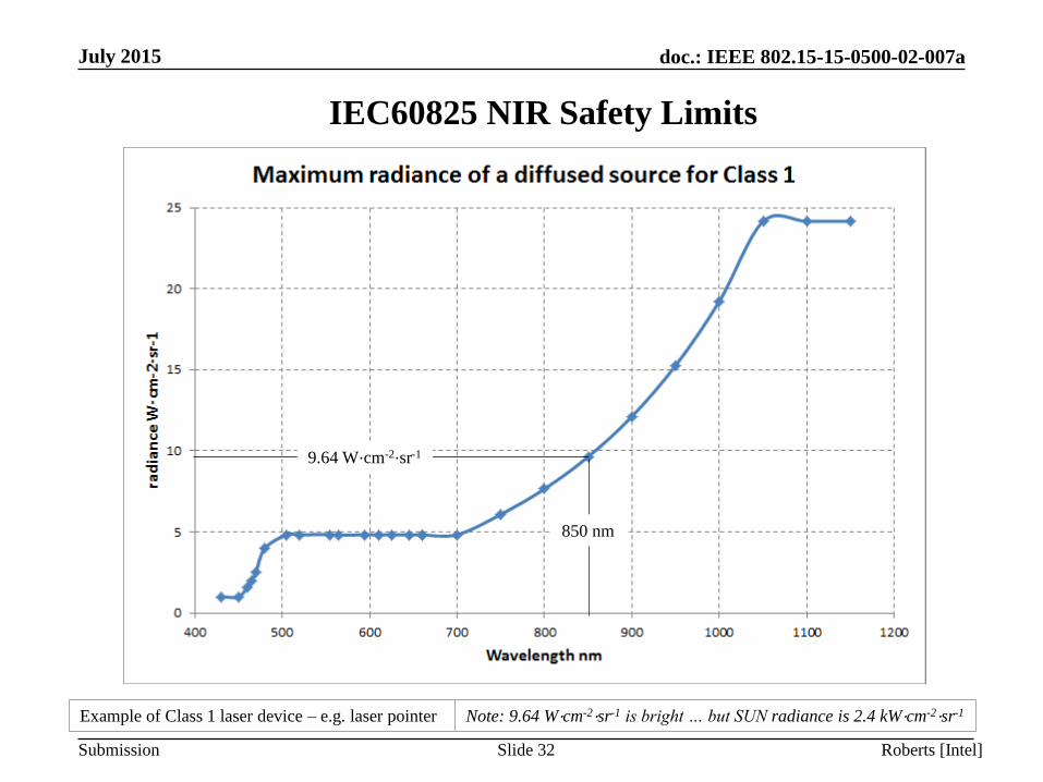
IEC60825 NIR Safety Limits
850 nm
9.64 W⋅cm-2⋅sr-1
Example of Class 1 laser device – e.g. laser pointer Note: 9.64 W⋅cm-2⋅sr-1 is bright … but SUN radiance is 2.4 kW⋅cm-2⋅sr-1

doc.: IEEE 802.15-15-0500-02-007a
Submission
July 2015
Roberts [Intel]Slide 33
ATX = 1 cm2
Adet
Interpretation of IEC60825 NIR Safety Limits
=1 det2
detdet, 1 AD
D
ATX
D
To a first order approximation …
… how much power is ingested by the detector?
WD
AAsr
srcm
WcmAP TXTXTX
2
detdet,2
2
det 6.96.9
Interpretation for a ATX = 1 cm2
2
det
D
ALchannel WAP TXTX 6.9
See appendix D for more discussion
on source intensity using solid angles.

doc.: IEEE 802.15-15-0500-02-007a
Submission
July 2015
Roberts [Intel]Slide 34
Receiver noise floor is a mixture of thermal noise and shot noise.
)()()( fSfSfS thermalshottotal
The biggest contributor to shot noise is the ambient solar spectral irradiance on a bright sunny day.
Receiver Noise
Sun spectral irradiance at 850 nm (sea level): 90 uW/cm2/nm
Short noise is caused by the random arrival time of photons from a light source.

doc.: IEEE 802.15-15-0500-02-007a
Submission
July 2015
Roberts [Intel]Slide 35
Impact of Fog Attenuation

doc.: IEEE 802.15-15-0500-02-007a
Submission
July 2015
Roberts [Intel]Slide 36
Dense Fog Thick Fog Moderate Fog
DD
ALLL mdBfogdBchanneldBtotal
2
detlog10
0.01
0.1
1
10
0 0.1 0.2 0.3 0.4 0.5 0.6 0.7 0.8 0.9 1
Att
en
ua
tio
n d
B/m
Visibility (V) km
850 nm Attenuation Per Meter in Fog

doc.: IEEE 802.15-15-0500-02-007a
Submission
July 2015
Roberts [Intel]Slide 37
Reaction Time and Stopping Distance ImplicationsAssumptions:
- road coefficient of friction: 0.8
- reaction time: 2.5 secs (typical)
- road grade: level
0
50
100
150
200
250
0 20 40 60 80 100 120 140 160
Vis
ibili
ty D
ista
nce
me
ters
km/hr
Visibility Distance vs. Speed
active cruise control range*
*http://www.bmw.com/com/en/insights/technology/technology_guide/articles/active_cruise_control_stop_go.html
http://easycalculation.com/engineering/civil/vehicle-stopping-distance.php
Automotive Industry
Dilemma: what to do
when the sensor
technology out performs
the human eye? Do we
encourage blind driving?

doc.: IEEE 802.15-15-0500-02-007a
Submission
July 2015
Roberts [Intel]Slide 38
Example Link Analysis ATX = cm2Adet = cm2
D
A detailed 850 nm link budget will be presented
as part of the Intel proposal to IEEE802.15.7r1.

doc.: IEEE 802.15-15-0500-02-007a
Submission
July 2015
Roberts [Intel]Slide 39
Appendices

doc.: IEEE 802.15-15-0500-02-007a
Submission
July 2015
Roberts [Intel]Slide 40
Appendix A
Ascertaining the LED parameters of interest
On the following pages, equation (2.2.1) and Figure 2.1.1 are from the book
Introduction to Solid-State Lighting by A. Zukauskas, et.al. The equation
relates the power spectral distribution S() (W/nm) to luminous flux v (lm).

doc.: IEEE 802.15-15-0500-02-007a
Submission
July 2015
Roberts [Intel]Slide 41
V() is the relative luminous efficiency function defined by CIE and given in the table
(from internet) and curve (from the book Fig 2.1.1)
780
380
683 ( ) ( )
nm
t t
nm
F S V d The LED total luminous flux Ft (lumens) is given as (2.2.1)
Sometimes it is convenient to use a Gaussian curve fitting for V() (from internet)
2285.4( 0.559)( ) 1.019 : inV e m ,
Find transmitted power and spectral density
Fig 2.1.1

doc.: IEEE 802.15-15-0500-02-007a
Submission
July 2015
Roberts [Intel]Slide 42
'( ) ( )t t tS c S
Typically we only know a normalized spectral curve St’() instead of St() in (2.2.1). Denote
their relation as St()=ct St’() with an unknown scaling factor ct that can be found from
780
'
380
683 ( ) ( )
tt nm
t
nm
Fc
S V d
Warm White
Neutral White
Cool White
780
'
380
683 ( ) ( )
nm
t t t
nm
F c S V d
Remark:
The above step to find St() can be
skipped if St() can be either
measured using a spectrometer or
supplied by the LED vendor.
780
380
( )
nm
t t
nm
P S d
H
L

doc.: IEEE 802.15-15-0500-02-007a
Submission
July 2015
Roberts [Intel]Slide 43
A normalized spatial luminous intensity distribution gt() is provided by a vendor.
We need to find the axial intensity I0 that is defined as the luminous intensity
(candelas) on the axis of the source (zero solid angle). Since the luminous flux Ft
is also a spatial integral of spatial luminous intensity in addition to spectral integral
we used before, we have the following relationmax max
0 0
0 0
* ( ) 2 ( )sint t tF I g d I g d
max0
0
2 ( )sin
t
t
FI
g d
where max and max are the source beam solid
angle and maximum half angle respectively and
max=2(1-cosmax).
normalized spatial luminous intensity distribution
Find transmitter luminous spatial intensity distribution I0 gt()
Note: if the axial intensity is provided by
the vendor then one only need convert
the intensity from candelas to watts/sr.

doc.: IEEE 802.15-15-0500-02-007a
Submission
July 2015
Roberts [Intel]Slide 44
Appendix B
Calculating Integrated Spectral Flex Density

doc.: IEEE 802.15-15-0500-02-007a
Submission
July 2015
Roberts [Intel]Slide 45
Flu
x /
ba
nd
wid
th (
W/n
m)
LED Spectrum
(white LED)
2
21150
250
)()()( RdLRSP
nm
nm
RX
Where T() is the transmitter power spectral density (W/nm)
R() is the detector responsivity (A/W at )
L() is the propagation loss (loss at )
The detector diode vendors are
giving us the info we needThis is the information we need
from the LED vendor
For best performance we want the detector spectral responsivity to be “matched” to
the LED spectral density. In general this is hard to due, especially for white LEDs.

doc.: IEEE 802.15-15-0500-02-007a
Submission
July 2015
Roberts [Intel]Slide 46
Appendix C
Receiver Noise Density Calculations
doc.: IEEE 802.15-15-0500-02-007a
Submission
July 2015
Roberts [Intel]Slide 47
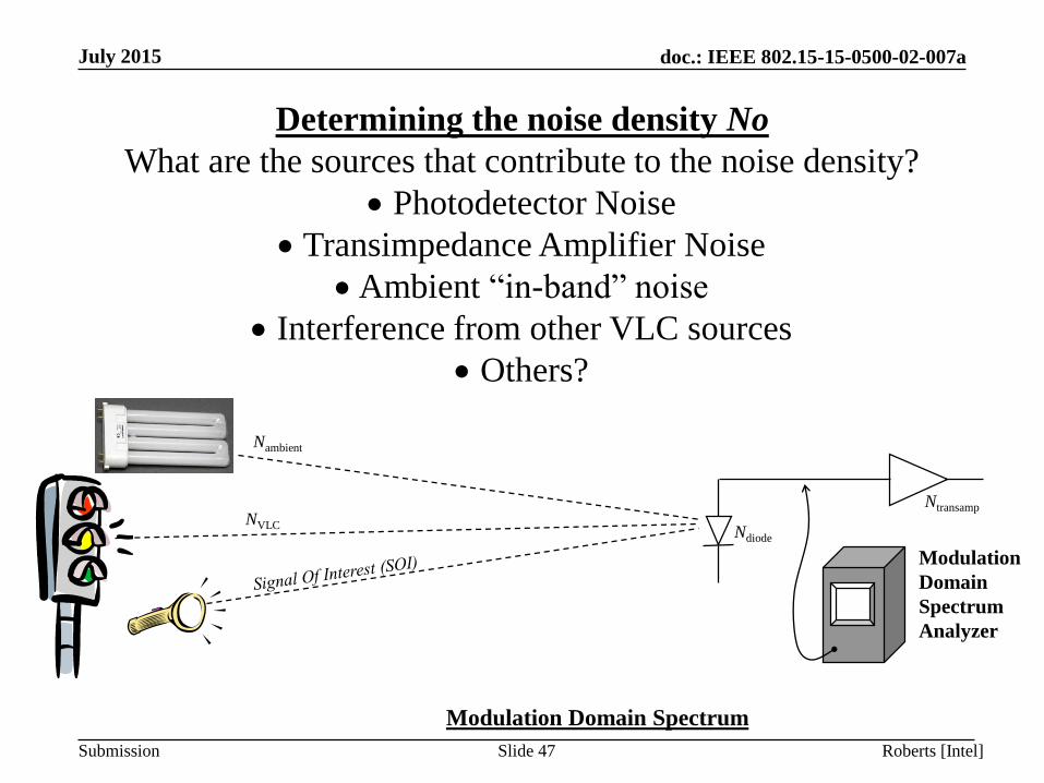
Determining the noise density No
What are the sources that contribute to the noise density?
Photodetector Noise
Transimpedance Amplifier Noise
Ambient “in-band” noise
Interference from other VLC sources
Others?
Ndiode
Ntransamp
Nambient
NVLC
Modulation Domain Spectrum
Modulation
Domain
Spectrum
Analyzer

doc.: IEEE 802.15-15-0500-02-007a
Submission
July 2015
Roberts [Intel]Slide 48
Ambient “In-Band” Noise Floor
This probably has to be empirically
measured for many different environments

doc.: IEEE 802.15-15-0500-02-007a
Submission
July 2015
Roberts [Intel]Slide 49
Interference from other VLC sources
For OCC this source of noise is unlikely because of
the angle-of-arrival mapping of the lens because the
interferer would have to be on the same angular
vector as the desired noise source. In general, an
interfering source will form an image elsewhere on
the image sensor and can be spatially filtered out.

doc.: IEEE 802.15-15-0500-02-007a
Submission
July 2015
Roberts [Intel]Slide 50
CL
R2
2 2 2 ( ) 4shotnpd thermal D S B SHi i i q I I I kT R
q is the electron charge (1.6e-19 coulombs)
ID is the dark current
IS is the signal current
IB is the background light induced current
B is the bandwidth (B=1 Hz for N0)
k is Boltzmann’s constant (1.38e-23 J/K)
T is the Kelvin temperature (~290 K)
RSH is the shunt resistance
The detector itself contributes a noise density Ndiode (W/ Hz)
(A/ Hz)
R2C2

doc.: IEEE 802.15-15-0500-02-007a
Submission
July 2015
Roberts [Intel]Slide 51
TI OPA111
R2=10e6 ohms
Transimpedance
Amplifier Noise Analysis
Ref. TI/Burr-Brown Application Bulletin SBOA060
“Noise Anaysis of FET Transimpedance Amplifiers”
Assume R3=0
http://focus.ti.com/lit/an/sboa060/sboa060.pdf

doc.: IEEE 802.15-15-0500-02-007a
Submission
July 2015
Roberts [Intel]Slide 52
The resistors and capacitors form
critical corner frequencies as shown
below:
2
2 2
1
2f
R C
2121 ||||2
1
CCRRfa
TI OPA111

doc.: IEEE 802.15-15-0500-02-007a
Submission
July 2015
Roberts [Intel]Slide 53
Typically op-amps have three noise regions … the above noise regions are for the TI
OPA111 op-amp. It is anticipated most outdoor VLC implementations will be
bandpass systems operating in noise region 3.
Noise Regions for the
TI OPA228

doc.: IEEE 802.15-15-0500-02-007a
Submission
July 2015
Roberts [Intel]Slide 54
The approximation output noise is given by
niRn NNNN 00
3
00
2
2
12
3
3
0 1
C
CKN n
20 4kTRN R
where
2
2
22
2
22
0 4)(2 RRkTIIIqiRiiN SHBSDnopnpdnop
in

doc.: IEEE 802.15-15-0500-02-007a
Submission
July 2015
Roberts [Intel]Slide 55
Then electrical SNR is
( ) ( ) ( )rH
rL
sig r f DI S R R d
The signal current is given as
2
2
2
2
2
2
12
3
2
2
04)(241
/)()()(
RRkTIIIqikTRC
CK
RatedLRSR
N
E
SHBSDnop
b
rH
rL

doc.: IEEE 802.15-15-0500-02-007a
Submission
July 2015
Roberts [Intel]Slide 56
2
2
2
2
2
2
12
3
2780
380
2
04)(241
/)()()(
RRkTIIIqikTRC
CK
RatedLRSR
N
E
SHBSDnop
nm
nmb
Hz
V
Hz
V 22
Hz
VsV
sA
J
s
sV
A
J
A
VK
K
J 2
Hz
V
A
V
Hz
A 222
Hz
VsVV
sC
CV
A
C
A
VAC
2222
2
2
/
Hz
V
sW
AW
A
V 22
1
1
Eb/No Dimensional Analysis
AVs
JW
sA
J
A
WV
s
CA
sA
J
A
V2
sHz
1
KT
KJk
coulombsCq
/
)(
Hz
V
AV
AV
KK
J 22

doc.: IEEE 802.15-15-0500-02-007a
Submission
July 2015
Roberts [Intel]Slide 57
Appendix D
Solid angle path loss model

doc.: IEEE 802.15-15-0500-02-007a
Submission
July 2015
Roberts [Intel]Slide 58
α
β
θmax
D
r
Transmitter
Receiver
LOS Link Model
The receiver distance to the source is D
The receiver aperture radius is r and receiver area is Ar
The angle between receiver normal and source-receiver line is
The angle between source beam axis and source-receiver line (viewing
angle) is
The solid angle of the receiver seen by the source is r

doc.: IEEE 802.15-15-0500-02-007a
Submission
July 2015
Roberts [Intel]Slide 59
The luminous angular intensity of the source at the receiver direction is
I0gt(), and therefore the receiver ingested luminous flux Fr=I0gt()r.
The luminous path loss can be represented as
where r is the receiver solid angle which satisfies Arcos()D2r .
max max max
0
2
0
0 0 0
( ) ( ) ( ) cos
2 ( )sin 2 ( )sin 2 ( )sin
t r t r t rrL
t
t t t
I g g g AFL
FI g d g d D g d
Power path loss Lp can be proven equal to luminous path loss LL as follows:
Optical power can be written as
In LOS free space propagation, path loss is assumed independent of
wavelength. Power path loss can be represented as Lp=S2()/S1()=P2/P1.
Luminous flux is related to S() as , which is
linear with S()
Therefore, LL=F2/F1=Lp.
( )H
L
P S d
683 / ( ) ( )H
L
F lm W S V d

doc.: IEEE 802.15-15-0500-02-007a
Submission
July 2015
Roberts [Intel]Slide 60
Now that we have known the optical power loss due to LOS propagation,
we can obtain the received optical spectral density from transmitter optical
spectral density as
Suppose we use a photodiode detector to
receive the signal light. We can obtain the
electrical power of the signal as
( ) ( ) ( )r p t L tS L S L S
The detector diode vendors are
giving us the info we need
Received optical power , ( ) ( ) rH
rL
r o r fP S R d
Find received optical and electrical power
( )D
qR
hc
21150
,
250
( ) ( ) ( )
nm
r e r r D L
nm
P S R R d R
f
where Sr() is the received light power spectral density (W/nm)
Rr() is the receiver filter spectral response
RD() is the detector responsivity (A/W at )

doc.: IEEE 802.15-15-0500-02-007a
Submission
July 2015
Roberts [Intel]Slide 61
ideal
typical
Exemplary Optical Filter Response
http://www.newport.com/images/webclickthru-EN/images/2226.gif

doc.: IEEE 802.15-15-0500-02-007a
Submission
July 2015
Roberts [Intel]Slide 62
Summary of key steps to obtain received optical
power and electrical power
• Calculate transmitter (source) optical power from given luminous
flux Ft (lumens) and normalized spectral curve St’()
• Find the transmitter axial intensity I0 from given luminous flux Ft
and luminous spatial intensity distribution gt()
• Find receiver ingested luminous flux Fr from receiver solid angle
and transmitter luminous spatial intensity distribution I0 gt()
• Find the luminous path loss LL from Ft and Fr
• Prove power path loss Lp is equal to luminous path loss LL from
which to find received optical power spectral curve Sr()
• Calculate received optical power and electrical power

doc.: IEEE 802.15-15-0500-02-007a
Submission
July 2015
Roberts [Intel]Slide 63
Appendix E
RX aperture and magnification factor
doc.: IEEE 802.15-15-0500-02-007a
Submission
July 2015
Roberts [Intel]Slide 64
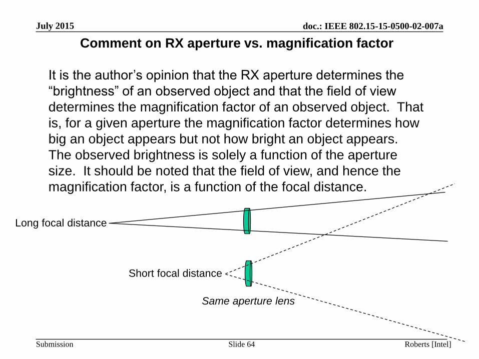
Comment on RX aperture vs. magnification factor
It is the author’s opinion that the RX aperture determines the
“brightness” of an observed object and that the field of view
determines the magnification factor of an observed object. That
is, for a given aperture the magnification factor determines how
big an object appears but not how bright an object appears.
The observed brightness is solely a function of the aperture
size. It should be noted that the field of view, and hence the
magnification factor, is a function of the focal distance.
Same aperture lens
Long focal distance
Short focal distance

doc.: IEEE 802.15-15-0500-02-007a
Submission
July 2015
Roberts [Intel]Slide 65
Magnification factor and power density
When viewing a light source, the magnification factor impacts the spatial
power density projected onto the image sensor. As mentioned previously, the
aperture determines how much power is ingested, but the magnification factor
(which is a function of the focal length) determines the image power density.
Case 2 … more magnification
• longer focal length
• image appears larger
• lower power density
Assumptions
• constant aperture
• ingested power is constant
Case 1 … less magnification
• shorter focal length
• image appears smaller
• higher power density

doc.: IEEE 802.15-15-0500-02-007a
Submission
July 2015
Roberts [Intel]Slide 66
∆𝑃𝐷= 𝑃 𝜋 ∙ 𝑀𝑟 2
𝑃 𝜋 ∙ 𝑟2=
1
𝑀2
The change in power density PD is related to magnification factor M as
The change in power density is inversely proportional to the square of
the magnification factor.

doc.: IEEE 802.15-15-0500-02-007a
Submission
July 2015
Roberts [Intel]Slide 67
Appendix F
Fog diffusion ‘glow’
“

doc.: IEEE 802.15-15-0500-02-007a
Submission
July 2015
Roberts [Intel]Slide 68
Fog causes light scattering in all directions. Forward scattering is
realized when the light initially reflects backwards then reflects one or
more times towards the forward direction. The net result is the light
appears to have a radial glow about an intense inner beam that is
attenuated as per Kim’s equation. The intensity of the radial glow is
inversely proportional to the Kim attenuation; that is, the inner core
attenuation is due to diffused light causing the radial glow.
Beam

doc.: IEEE 802.15-15-0500-02-007a
Submission
July 2015
Roberts [Intel]Slide 69
Inner Core Attenuation as per Kin’s modified equation (negative gain ratio) …
Α 𝑘𝑚 𝑏𝑒𝑎𝑚 = 𝑒−
3.91𝑉
𝜆550 𝑛𝑚
−𝑞
Proportional total glow intensity approximation (ratio) …
Α 𝑘𝑚 𝑔𝑙𝑜𝑤 = 1 − 𝑒−
3.91𝑉
𝜆550 𝑛𝑚
−𝑞
The intensity of the glow off the main beam is proportional to the ratio squared of the
beam radius r to the distance d.
r
d
The glow at the point of interest is approximated as:
Ratio: Α 𝑘𝑚 𝑝𝑜𝑖𝑛𝑡_𝑔𝑙𝑜𝑤 =𝑟
𝑑
21 − 𝑒
−3.91
𝑉
𝜆
550 𝑛𝑚
−𝑞
dB: Α 𝑑𝐵/𝑘𝑚 𝑝𝑜𝑖𝑛𝑡_𝑔𝑙𝑜𝑤 = 10 ∗ 𝑙𝑜𝑔10𝑟
𝑑
21 − 𝑒
−3.91
𝑉
𝜆
550 𝑛𝑚
−𝑞

doc.: IEEE 802.15-15-0500-02-007a
Submission
July 2015
Roberts [Intel]Slide 70
The signal to glow ratio (i.e. ratio between a point in the main beam with radius r to a
point off the main beam at distance d) is given as (for 1 km distance) …
𝑅 𝑘𝑚 𝑆𝐺𝑅 =𝑒−
3.91𝑉
𝜆550 𝑛𝑚
−𝑞
𝑟𝑑
21 − 𝑒
−3.91𝑉
𝜆550 𝑛𝑚
−𝑞 =𝑑
𝑟
2𝑒−
3.91𝑉
𝜆550 𝑛𝑚
−𝑞
1 − 𝑒−
3.91𝑉
𝜆550 𝑛𝑚
−𝑞
𝑅𝑑𝐵 𝑘𝑚 𝑆𝐺𝑅 = 10 ∗ 𝑙𝑜𝑔10𝑑
𝑟
2𝑒−
3.91𝑉
𝜆550 𝑛𝑚
−𝑞
1 − 𝑒−
3.91𝑉
𝜆550 𝑛𝑚
−𝑞 .
These results need to be scaled for arbitrary (presumably less) distance.

doc.: IEEE 802.15-15-0500-02-007a
Submission
July 2015
Roberts [Intel]Slide 71
The SGR results (signal to glow ratio) are currently for 1 km distance but needs to be
scaled for more practical shorter distances, and the results should also include the
directivity introduced by the camera’s field of view. We can realize the former by
introducing an exponential scaling term based upon the operational distance L and the
latter by approximating the field of view via an inverse cosine scaling term.
Beam Camera #1
Camera #2
d
L

doc.: IEEE 802.15-15-0500-02-007a
Submission
July 2015
Roberts [Intel]Slide 72
The modified SGR results are then given by
𝑅 𝑘𝑚 𝑆𝐺𝑅 =𝑑
𝑟
2
∙𝑒−
3.91𝑉
𝜆550 𝑛𝑚
−𝑞 𝐿 1000
1 − 𝑒−
3.91𝑉
𝜆550 𝑛𝑚
−𝑞 𝐿 1000
∙1
𝑐𝑜𝑠 𝑡𝑎𝑛−1𝑑𝐿
.
The results are expressed in dBs as
𝑅𝑑𝐵 𝑘𝑚 𝑆𝐺𝑅 = 10 ∗ 𝑙𝑜𝑔10𝑑
𝑟
2
∙𝑒−
3.91𝑉
𝜆550 𝑛𝑚
−𝑞 𝐿 1000
1 − 𝑒−
3.91𝑉
𝜆550 𝑛𝑚
−𝑞 𝐿 1000
∙1
𝑐𝑜𝑠 𝑡𝑎𝑛−1𝑑𝐿
.

doc.: IEEE 802.15-15-0500-02-007a
Submission
July 2015
Roberts [Intel]Slide 73
-10
-5
0
5
10
15
20
25
30
35
40
0.01 0.1 1 10
Sig
na
l to
Glo
w R
atio
dB
Visibility (V) Km
Signal to Glow Ratio
Example assumptions …
• Wavelength: 850 nm
• Beam Radius: 1m
• Off beam distance “d”: 3m
• Standoff length “L”: 10m