jumps in rank and expected returns: introducing varying cross-sectional risk

7/28/2019 Jumps in Rank and Expected Returns: Introducing Varying Cross-sectional Risk

http://slidepdf.com/reader/full/jumps-in-rank-and-expected-returns-introducing-varying-cross-sectional-risk 1/33

Jumps in Rank and Expected Returns:

Introducing Varying Cross-sectional Risk∗

Gloria González-RiveraDepartment of Economics

University of California, Riverside

Tae-Hwy LeeDepartment of Economics

University of California, Riverside

Santosh MishraDepartment of EconomicsOregon State University

Abstract

We propose an extension of the meaning of volatility by introducing a measure, namely theVarying Cross-sectional Risk (VCR), that is based on a ranking of returns. VCR is definedas the conditional probability of a sharp jump in the position of an asset return within thecross-sectional return distribution of the assets that constitute the market, which is representedby the Standard and Poor’s 500 Index (SP500). We model the joint dynamics of the cross-sectional position and the asset return by analyzing (1) the marginal probability distribution of a sharp jump in the cross-sectional position within the context of a duration model, and (2) theprobability distribution of the asset return conditional on a jump, for which we specify diff erentdynamics in returns depending upon whether or not a jump has taken place. As a result, the

marginal probability distribution of returns is a mixture of distributions. The performance of our model is assessed in an out-of-sample exercise. We design a set of trading rules that areevaluated according to their profitability and riskiness. A trading rule based on our VCR modelis dominant providing superior mean trading returns and accurate Value-at-Risk forecasts.

Key words : Cross-sectional position, Duration, Leptokurtosis, Momentum, Mixture of normals,Nonlinearity, Risk, Trading rule, VaR, VCR.

JEL Classi fi cation : C3, C5, G0.



1 Introduction

Economists, investors, regulators, decision makers at large face uncertainty in a daily basis. While

most of us share an intuitive notion on the meaning of uncertainty, which involves future events and

their probability of occurrence, the measurement of uncertainty depends on who you are and what

you do. For instance, financial economists and econometricians for most part equate uncertainty

with risk, risk with volatility, and volatility with variance (or any other measure of dispersion).

Investors and regulators are not only concerned with measures of volatility but also they monitorthe tails of the probability distribution of returns. Regulators worry about catastrophic or large

losses that can jeopardize the health of the financial system of the economy. Decision theorists

deal with volatility measures only in particular instances since the variance may not be a sufficient

statistic to summarize the risk faced by an agent, and often they claim that an ordinal measure of

risk, i.e. the construction of a ranking of assets, may be sufficient for an agent to make a rational

choice under uncertainty (Granger, 2002).

In this paper we put forward a diff erent measure of volatility that combines the views of the

variance advocates with those of the ranking advocates. For financial assets, our conception of risk

is based on an ordinal measure (the cross-sectional ranking of an asset in relation to its peers) and

on a cardinal measure (the univariate conditional volatility of the asset). A graphical introduction

to our main idea is contained in Figure 1, where we present a stylized description of the problem that

we aim to analyze. Let yi,t be the asset excess return of firm i at time t, and zi,t the cross-sectional

position (percentile ranking) of this return in relation to all other assets that constitute the market.

For every t, we observe the realizations of all asset returns, and for each asset, we assign a cross

sectional position zi,t. For one period to the next, the cross-sectional position changes. In Figure

1, we draw a histogram to represent the ranking of realized asset returns, which is time-varying.

Our objective is to model the dynamics of the cross-sectional position jointly with the dynamics

of the asset return. To illustrate the diff erent dynamics of yi,t and zi,t, we choose four points in

time. Consider the movements of yi,t and zi,t going from t1 to t4. We observe that from t1 to t2,

the market overall has gone down as well as the return and the cross-sectional position of asset



We are interested in this notion of relative risk. Note that the time series yi,t conveys univariate

information about asset i but the time series zi,t implicitly conveys information about the full

market and, in this sense, it is a multivariate measure.

We set our problem as to model the joint distribution of the return and the probability of a

(sharp) jump (J i,t) in the cross-sectional position of the asset zi,t, i.e. f (yi,t, J i,t|F t−1) where F t−1 is

an information set up to time t − 1. Since f (yi,t, J i,t|F t−1) = f 1(J i,t|F t−1)f 2(yi,t|J i,t,F t−1), our task

will be accomplished by modelling the marginal distribution of the jump and the conditional dis-

tribution of the return. The former provides the conditional probability of jumping cross-sectional

positions, which we call the time-Varying Cross-sectional Risk (VCR). It is straightforward to

understand that VCR is time-varying because it depends on an information set that changes over

time, and that it conveys cross-sectional information because it depends on the position of the asset

in relation to its peers. We say that is risk because the probability of a sharp jump in cross-sectional

positions is an assessment of the chances of being a winner or a loser within the available set of assets in the market.

On modelling f 1(J i,t|F t−1), our paper also connects with the recent literature in microstructure

of financial markets and duration analysis (Engle and Russell, 1998). This line of research aims to

model events (e.g., trades) and waiting times between events. The traditional question in duration

analysis is what is the expected length of time between two events given some information set. In

this paper, the event is the jump in the cross-sectional position of the asset return, however, when

we model the expected duration between jumps or its mirror image —the conditional probability

of the jump—, our analysis is performed in calendar time as in Hamilton and Jordà (2002). Given

some information set, the question of interest is what is the likelihood that tomorrow there will be

a sharp change in the position of this firm in relation to the cross-sectional distribution of returns.

This calendar time approach is necessary because asset returns are reported in calendar time (days,

weeks, etc.) and it has the advantage of incorporating other information available in calendar time.

Furthermore, the modelling of f 1(J i,t|F t−1) also connects with the financial literature on “mo-

mentum”. At time t, a typical momentum strategy consists of buying stocks that have performed



near future, that is winners (losers) continue to be winners (losers). It is natural to think that this

type of persistence or time patterns must be a target for statistical modeling and may be exploited

from a forecasting point of view. If we model the conditional probability of a sharp jump in cross

sectional position and calculate its inverse, we are assessing the conditional expected duration of a

high (low) position in the cross-sectional ranking of assets.

The ultimate justification of any time series model is its forecasting ability. The model that

we propose is highly nonlinear and its performance is assessed in an out-of-sample exercise within

the context of investment decision making. We consider two criteria. In the first, we deal with an

investor whose interest is to maximize profits of a portfolio long in stocks. The second criterion is

to consider an investor who worries about potential large losses and wishes to add a Value-at-Risk

evaluation to her trading strategy. Profitability and riskiness are the two coordinates in the mind

of the investor. We design a set of trading rules that will be compared in the two aforementioned

criteria. The statistical comparison is performed within the framework of White’s (2000) realitycheck, which controls for potential data snooping biases. A trading rule that exploits the one-step

ahead forecast of the cross-sectional positions of asset returns will be shown to be clearly superior

to other rules based on more standard models.

The organization of the paper is as follows. In section 2, we provide our strategy for the joint

modelling of asset returns and jumps in the cross-sectional position. We present the estimation

results for a sample of weekly returns of those SP500 firms that have survived for the last ten years.

In section 3, we assess the out-of-sample performance of our model. We explain the trading rules,

loss functions, and the statistical framework to compare diff erent trading rules. Finally, in section

4 we conclude.

2 Cross-sectional position and expected returns

In this section, we propose a bivariate model of expected returns and jumps in the ranking of a

given asset within the cross-sectional distribution of asset returns.

Let yi,t be the return of the ith firm at time t, and yi,tM i=1 be the collection of asset returns of



to the return of the ith firm. We write

zi,t ≡ M −1M X j=1

1(y j,t ≤ yi,t), (1)

where 1(·) is the indicator function, and for M large, zi,t ∈ (0, 1] In Figure 1, zi,t is the shaded

area of the cross-sectional histogram of returns. We say that a (sharp) jump in the cross-sectional

position of the ith firm has occurred when there is a minimum (upwards or downwards) movement

of 0.5 in the cross-sectional position of the return of the ith firm. We define such a jump as a binary

variable

J i,t ≡ 1(|zi,t − zi,t−1| ≥ 0.5). (2)

The choice of the magnitude of the jump is not arbitrary. The sharpest jump that we could consider

is 0.5. In every time period, we need to allow for the possibility of jumping, either up or down,

in the following period regardless of the present position of the asset. For instance, if we choose

a jump greater than 0.5, say 0.7, and zi,t = 0.4, then the probability of jumping up or down in

the next time period is zero. Note that the defined jump does not imply that the return will be

above or below the median. As an example, if zi,t−1 = 0.4 and zi,t = 0.6, then J i,t = 0 but the

return at time t will be above the cross-sectional median of returns. However, if J i,t = 1, then

the asset return has moved either above or below the median. Note that an upward (downward)

jump implies neither a higher (lower) return, nor a larger (smaller) variance. This is so because the

cross-sectional position is the result of the interaction of the relative movements of all individual

assets in the market. Moreover our definition of jump is diff erent from the jump process that

can be defined in the univariate return process (e.g., Aït-Sahalia 2003). Our jump is a jump in

cross-sectional positions, which implicitly depends on numerous univariate return processes.

Our objective is to model the conditional joint probability density function of returns and jumps

f (yi,t, J i,t|F t−1; θ), where F t−1 is the information set up to time t−1, which contains past realizations

of returns, jumps, and cross-sectional positions. To simplify notation, we drop the subindex i but

in the following analysis should be understood that the proposed modelling is performed for every



where θ = (θ0

1 θ0

2)0. For a sample yt, J tT t=1, the joint log-likelihood function is

T Xt=1

log f (yt, J t|F t−1; θ) =T Xt=1

log f 1(J t|F t−1; θ1) +T Xt=1

log f 2(yt|J t,F t−1; θ2).

Let us call L1(θ1) =PT

t=1 log f 1(J t|F t−1; θ1) and L2(θ2) =PT

t=1 log f 2(yt|J t,F t−1; θ2). The max-

imization of the joint log-likelihood function can be achieved by maximizing L1(θ1) and L2(θ2)

separately without loss of efficiency if the parameter vectors θ1 and θ2 are “variation free” in the

sense of Engle et al. (1983) as is the case in our set-up below.

2.1 Modelling the cross-sectional jump f 1(J t|F t−1; θ1)

In order to model the conditional probability of jumping, we define a counting process N (t) as the

cumulative number of jumps up to time t, that is, N (t) =Pt

n=1 J n. This is a non-decreasing step

function that is discontinuous to the right and to the left and for which N (0) = 0. Associated with

this counting process, we define a duration variable DN (t) as the number of periods between two

jumps. Note that because our interest is to model the jump jointly with returns and these are

recorded in a calendar basis (daily, weekly, monthly, etc.), the duration variable needs to be defined

in calendar time instead of event time as is customary in duration models. The question of interest

is, what is the probability of a sharp jump at time t in the cross-sectional position of the ith firm

asset return given all available information up to time t − 1? This is the conditional hazard rate pt

pt ≡ Pr(J t = 1|F t−1) = Pr(N (t) > N (t − 1)|F t−1), (3)

which we call the time-varying cross-sectional risk (VCR). From (3), we note that VCR is time-

varying because it depends on the information set F t−1, and it is cross-sectional because J t depends

on the positioning of the asset return in relation to the other firms in the market. Furthermore,

because J t = 1, VCR assesses the possibility of being in the upper tail (winner) or in the lower

tail (loser) of the cross-sectional distribution of asset returns. In this sense, we called this measure

“risk”.

It is easy to see that the probability of jumping and duration must have an inverse relationship.



specify an autoregressive conditional hazard (ACH) model.1 A general ACH model is specified as

ΨN (t) =mX

j=1

α jDN (t)− j +rX

j=1

β jΨN (t)− j. (4)

Since pt is a probability, it must be bounded between zero and one. This implies that the conditional

duration must have a lower bound of one. Furthermore, working in calendar time has the advantage

that we can incorporate information that becomes available between jumps and can aff ect the

probability of jumping in future periods. We can write a general conditional hazard rate as

pt = [ΨN (t−1) + δ 0

X t−1]−1, (5)

where X t−1 is a vector of relevant calendar time variables such as past cross-sectional positions and

past returns.

The log-likelihood function L1(θ1) = PT t=1 log f 1(J t|F t−1; θ1) corresponding to a sample of

observed jumps in the cross-sectional position is

L1(θ1) =T Xt=1

[J t log pt(θ1) + (1 − J t) log(1 − pt(θ1))] , (6)

where θ1 = (α0,β 0, δ 0)0 is the parameter vector for which the log-likelihood function is maximized.

2.2 Modelling the return conditional on jumps f 2(yt|J t,F t−1; θ2)

We assume that the return to the ith firm asset may behave diff erently depending upon the occur-

rence of a sharp jump. If a sharp jump has occurred, the return was pushed either towards the

lower tail or upper tail of the cross-sectional distribution of returns. In relation to the market, this

asset becomes either a loser or a winner. A priori, one may expect diff erent dynamics in these two

states. A general specification is

f 2(yt|J t,F t−1; θ2) =

½N (µ1,t, σ21,t) if J t = 1,

N (µ0,t, σ20,t) if J t = 0,(7)

where µt is the conditional mean and σ2t is the conditional variance, potentially diff erent depending



skewed (right skewed) distribution of returns would be appropriate when a downward (upward)

jump has taken place. This is not the case. Remember that whether a jump happens is a function

of the state of the market. One may think of a bullish market where a downward jump in the

cross-sectional position of a particular asset could be associated with a high return (in the right

tail of the return distribution), and on the contrary, in a bearish market an upward jump may be

associated with a low return (in the left tail of the return distribution). Consequently, our assump-

tion of symmetry (normality) is justified whether the jump is upward or downward. However, more

complex distributions can be assumed.

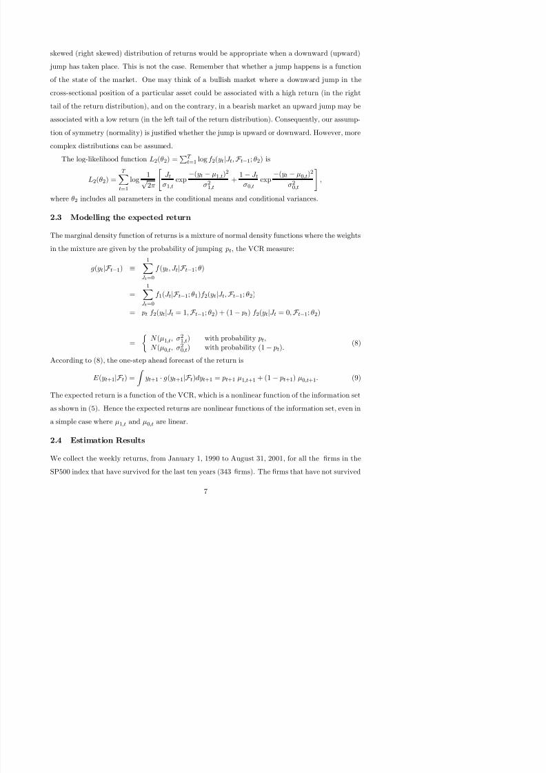
The log-likelihood function L2(θ2) =PT

t=1 log f 2(yt|J t,F t−1; θ2) is

L2(θ2) =T Xt=1

log1√ 2π

"J tσ1,t

exp−(yt − µ1,t)

2

σ21,t+

1 − J tσ0,t

exp−(yt − µ0,t)

2

σ20,t

#,

where θ2 includes all parameters in the conditional means and conditional variances.

2.3 Modelling the expected return

The marginal density function of returns is a mixture of normal density functions where the weights

in the mixture are given by the probability of jumping pt, the VCR measure:

g(yt|F t−1) ≡1X

J t=0

f (yt, J t|F t−1; θ)

=1X

J t=0

f 1(J t|F t−1; θ1)f 2(yt|J t,F t−1; θ2)

= pt f 2(yt|J t = 1,F t−1; θ2) + (1 − pt) f 2(yt|J t = 0,F t−1; θ2)

=

½N (µ1,t, σ21,t) with probability pt,

N (µ0,t, σ20,t) with probability (1 − pt).(8)

According to (8), the one-step ahead forecast of the return is

E (yt+1|F t) =

Z yt+1 · g(yt+1|F t)dyt+1 = pt+1 µ1,t+1 + (1 − pt+1) µ0,t+1. (9)

The expected return is a function of the VCR, which is a nonlinear function of the information set

h i (5) H th t d t li f ti f th i f ti t i



during this period are usually very volatile firms and tend to reside in the tails of the cross-sectional

distribution of asset returns, thus they will not aff ect substantially the cross-sectional positions of

the surviving firms. The total number of observations is 599. In Table 1, we summarize the un-

conditional moments (mean, standard deviation, coefficient of skewness, and coefficient of kurtosis)

for the 343 firms. The frequency distribution of the unconditional mean seems to be bimodal with

two well defined groups of firms, a cluster with a negative mean return of approximately −0.25%,

and another with a positive mean return of 0.25%. For the unconditional standard deviation, the

median value is 4.37. The median coefficient of skewness is 0.01, with most of the firms exhibiting

moderate to low asymmetry. All the firms have a large coefficient of kurtosis with a median value is

5.23. We calculate the Box-Pierce statistic to test for up to fourth order autocorrelation in returns

and we find mild autocorrelation for about one-third of the firms. However, the Box-Pierce test

for up to fourth order autocorrelation in squared returns indicates strong dependence in second

moments for all thefi

rms in the SP500 index.

[Table 1 about here]

2.4.1 The duration model

For 343 firms, we fit a conditional duration model as in (4) and (5). The information set con-

sists of past durations, past returns and past cross-sectional positions : DN (t)− j, yt− j , zt− j for j = 1, 2, . . . . The duration time series for every firm is characterized by clustering — long (short)

durations are followed by long (short) durations — and, consequently the specification of an ACH

model may be warranted. We maximize the log-likelihood function (6) with respect to the pa-

rameter vector θ1 = (α0,β 0, δ 0)0. We estimate diff erent lag structures (linear and nonlinear) of the

information set and, based on standard model selection criteria (t-statistics and log-likelihood ratio

tests), we obtain the following final specification

pt = [ΨN (t−1) + δ 0

X t−1]−1,

ΨN (t) = αDN (t)−1 + β ΨN (t)−1,



firms. All the parameters are statistically significant at the customary 5% level with the exception

of δ 4, for which do not report its frequency distribution.


For α, the median is 0.36 with 90% of the firms having an α below 0.48. For β , its frequency

distribution is highly skewed to the right with a median of 0.06 and with 90% of the firms having a

β below 0.25. The median persistence is 0.45 and for 90% of the firms, the persistence is below 0.63.

The estimates δ 2 and δ 3 have opposite signs, the former is positive and the latter is negative with

δ 2 being larger in magnitude than δ 3. The eff ect of δ 2 and δ 3 in expected duration depends on the

interaction between the cross-sectional position and the sign of the return. There are four possible

scenarios. For instance, when the past asset return is positive and below (above) the median

market return, its expected duration is longer (shorter) and the probability of a sharp jump is

smaller (larger), other things equal. On the contrary, when the past asset return is negative

and below (above) the median market return, its expected duration is shorter (longer) and the

probability of a sharp jump is larger (smaller), other things equal. Both δ 2 and δ 3 have a very

skewed cross-sectional frequency distributions. For δ 2, the median value is 0.15 with 90% of the

firms having a δ 2 below 0.55. For δ 3, the median value is −0.11 with 90% of the firms having a

δ 3 above -0.45. Roughly speaking, for a representative firm with median parameter estimates, the

expected duration is between 4 and 5 weeks, and since E ( pt) ≥ [E (ΨN (t−1)+δ 0

X t−1)]−1 by Jensen’s

inequality, a lower bound for the expected VCR is between 0.20 and 0.25.

In the last section of Table 2, we also report the median estimates of the parameters of the

duration model for the industrial sectors that are represented in the SP500 index. There are ten

sectors in the index, which have been reduced to eight. 2 The largest shares correspond to the

Consumer Goods sector with 28% of the SP500 companies, and the Information Technology sector

with 21% of the firms. The smallest share corresponds to the Energy sector with 5% of the firms.

The column denoted as α + β provides the median persistence in duration for each sector. A

high persistence implies longer expected durations, thus a lower probability of a sharp jump. The



of the calendar variables on the probability of a jump. Ceteris paribus, a low absolute value of the

estimate denotes a lower tendency of the asset return to move towards the median of the market.

As the volatile stocks are usually found in the tails of the cross-sectional distribution of the market,

a low absolute value of the estimate implies a tendency to remain in the lower or upper tail of

the cross-sectional distribution. We find that the Information Technology sector has the smallest

absolute values of δ 2 and δ 3 and the Utilities sector the largest, indicating that the latter is a

median performer compared to the former which has a tendency to move towards the tails of the

cross-sectional distribution of returns. The joint eff ect of duration persistence and impact of the

calendar variables is summarized in the column labeled ˆ pt, which is the median probability of a

sharp jump in each sector. Not surprisingly, the Information Technology sector has the largest

median probability with ˆ pt = 0.30, which means that about every three weeks these stocks jump

from the top (bottom) to the bottom (top) of the cross-sectional distribution of the market. On

the other side of the spectrum, we have the Utilities sector with the smallest median probabilityˆ pt = 0.11, which implies jumps every nine weeks approximately.

2.4.2 The nonlinear model for conditional returns

We proceed to estimate (7). Since this model is already nonlinear, we restrict the specification of the

conditional mean and conditional variance in each state (J t = 1 or J t = 0) to parsimonious linear

functions of the information set. After customary specification tests, the preferred specification of

the conditional first two moments is

µ1,t ≡ E (yt|F t−1, J t = 1) = ν 1 + γ 1yt−1 + η1zt−1,

µ0,t ≡ E (yt|F t−1, J t = 0) = ν 0 + γ 0yt−1 + η0zt−1,

σ2

1,t= σ2

0,t= σ2

t

= E (ε2

t

|F t−1, J t) = ω + ρε2

t−1

+ τσ2

t−1

,

(10)

where εt−1 ≡ (yt−1 − µ1,t−1)J t−1 + (yt−1 − µ0,t−1)(1 − J t−1). We arrive to this specification by

implementing a battery of likelihood ratio tests for the two null hypotheses:

H1 : µ1,t = µ0,t and H

2 : σ21,t = σ20,t.



normals. Within our model (10), the well known unconditional leptokurtosis of asset returns is

explained by the mixture of distributions.

The estimation results for the 343 firms are summarized in Table 3. We report the cross-sectional

frequency distributions of the parameters estimates of the conditional mean and conditional vari-

ance. The majority of the parameters are statistically significant at the 5% level.


When we consider asset returns for which a sharp jump has taken place, the impact of past

returns, γ 1, is predominantly negative (in 75% of the firms γ 1 < 0). The eff ect of past cross-

sectional positions, η1, is clearly negative for all the firms. These signs are expected. Consider

an asset for which a sharp jump has taken place (J t = 1), and whose past return has been going

down (∆yt−1 < 0). A movement down in past returns implies that the likelihood of a sharp jump

increases. Given that we are considering an asset for which a sharp jump is happening, we should

expect that the most likely direction of the jump is up, thus increasing the present expected return.

The same type or argument goes through when we consider movements in the cross-sectional

position. When there is no jump, the marginal eff ect of past returns, γ 0, on expected returns could

be positive or negative across the firms with a median value of 0.15. On the contrary, the marginal

eff ect of past cross-sectional positions, η0

, is clearly positive. This means that asset returns who

move up in the cross-sectional ranking of firms, but who have not experienced a sharp jump, tend

to have an increase in their expected returns, other things equal. For individual firms we observe

that |γ 1| > |γ 0| and |η1| > η0, which is consistent with the notion that, most of the time, sharp

jumps in cross-sectional positions must be associated with large movements in expected returns.

The median value of γ 1 is −1.11 compared to the median of γ 0 that is 0.15; and the median of

η1 is −0.61 compared to the median of η0 that is 0.37. We also report the median estimates for

every industrial sector represented in the SP500 index. The most salient feature is the behavior of

the Utilities sector. The median estimate of γ 1(γ 0) is very small (large) compared to that of other

sectors meaning that jumps in the Utilities sector are not very frequent corroborating the results of



is 0.93, with a median value for ρ of 0.06 and a median value for τ of 0.87. A leverage eff ect in

the conditional variance does seem to be warranted, the diff erent specifications of the conditional

mean across states take care of potential asymmetries in returns. We run standard diagnostic

checks such as the Box-Pierce statistics for autocorrelation in residuals, squared residuals, and

standardized squared residuals and we conclude that the residuals, standardized residuals, and

standardized squared residuals seem to be white noise. The specification (10) passes standard

diagnostic checks for model adequacy. However, given the nonlinearity of the model, a more drastic

check on the validity of the model is the assessment of its forecasting performance, which we analyze

in the following section.

3 Out-of-sample evaluation of the VCR model

In this section we assess the performance of the proposed VCR model within the context of invest-

ment decision making. We consider two major scenarios. First, we deal with an investor whose

interest is to maximize profits from trading stocks. We assume that her trading strategy — what to

buy, what to sell — depends on the forecast returns based on the VCR model in (9) and (10). This

trading strategy will be called VCR-Mixture Position Trading Rule and it is based on the one-step

ahead forecast of individual asset returns based on the VCR model. The superiority of the proposed

specification depends on its potential ability to generate larger profits than those obtained with

more standard models. In the second scenario, in addition to the profits (returns), the investor

wishes to assess potential large losses by adding a Value-at-Risk evaluation of her trading strategy.

In this case, the modelling of the conditional variance becomes also relevant. Both scenarios provide

an out-of-sample evaluation of the VCR model.

We proceed as follows. For each firm i in the market (343 firms), we compute the one-step

ahead forecast yi,t+1 of the return as in (9). The sequence of one-step ahead forecasts is obtained

with a “rolling” sample. For a sample size of T and with the first R observations, we estimate

the parameters of the model θR and compute the one-step ahead forecast yi,R+1(θR). Next, using

observations 2 to R + 1, we estimate the model again to obtain θR+1 and calculate the one-step



is,

zi,t+1 = M −1M X j=1

1(y j,t+1 ≤ yi,t+1), t = R, . . . , T − 1,

and buys the top K performing assets if their return is above the risk-free rate. In every subsequent

out-of-sample period (t = R, . . . , T − 1), the investor revises her portfolio, selling the assets that

fall out of the top performers and buying the ones that rise to the top, and she computes the

one-period portfolio return

πt+1 = K −1M X j=1

y j,t+1 · 1(z j,t+1 ≥ zK t+1), t = R, . . . , T − 1,

where zK t+1 is the cutoff cross-sectional position to select the K best performing stocks such that

PM j=1 1(z j,t+1 ≥ zK

t+1) = K . We form a portfolio with the top 1% performers in the SP500 index.

Every asset in the portfolio is weighted equally.

3.1 Competing trading rules

To evaluate the out-of-sample performance of the VCR model, we compare it with that of various

competing models.

A simple alternative to the VCR-mixture rule may be constructed by imposing H1 : µ1,t = µ0,t

in (10). This trading rule assesses the importance of the nonlinearity in expected returns. It will be

called Position Trading Rule because it takes into account the cross-sectional position of an asset

while it ignores the nonlinearity of the model (mixture of normal densities) for expected returns.

The one-step ahead forecast for every asset in the market is obtained from a linear specification of

the conditional mean where the regressors are past returns and past cross-sectional positions. As

in the previous rule, the ordinal position is predicted and a rolling sample scheme is used to obtainthe sequence of one-step ahead forecasts. The investor follows the same strategy as before buying

the top five performing assets and revising her portfolio in every period.

The third trading rule is a buy-and-hold strategy of the market portfolio. At the beginning of

h f i i l h i b h SP500 i d d h ld i il h d f h i l



previous price, and the best forecast for the return of any given asset is zero. Hence πt = 0 for any

t and any asset.

In summary, these four trading rules aim to assess the predictability of stock returns: the VCR-

Mixture Position Trading Rule claims that stock returns are non-linearly predictable, the Position

Trading Rule claims that stock returns are linearly predictable, the Random Walk Hypothesis

claims that stock returns are non-predictable, and the Buy-and-Hold-the-Market Trading Rule

claims that actively managed portfolios have no advantage over passively index investing.

3.1.1 Technical trading rules

In addition to the above four models, we also consider four classes of technical trading rules con-

sidered by Sullivan, Timmermann and White (1999). All the trading rules are based on the SP500

index. For each of the four technical trading rules below, we consider four parameterization.

Filter-Rule (x): If the weekly closing price of a particular security moves up at least x per cent,

buy and hold the security until its price moves down at least x per cent from a subsequent high,

at which time simultaneously sell and go short. The short position is maintained until the weekly

closing price rises at least x per cent above a subsequent low at which time one covers and buys.

The neutral position is obtained by liquidating a long position when the price decreases y percent

from the previous high, and covering a short position when the price increases y percent from the

previous low. We apply one of the rules of Sullivan et al. (1999) to define subsequent high (low).

A subsequent high (low) is the highest (lowest) closing price achieved while holding a particular

long (short) position. We also allow for the holding of the asset for c weeks ignoring any signals

generated from the market. We consider x : 0.05, 0.10, 0.20, 0.50, y = 0.5x, and c = 1.

Moving-Average-Rule (l, s): This rule involves going long (short) when the short period moving

average (s) rises above (falls below) the long period moving average (l). Its idea is to smooth outthe series and locate the initiation of trend (when s penetrates l). We consider four sets of local

moving averages with (l, s) : (10, 2), (20, 2), (10, 4), (20, 4), a fixed percentage band filter to rule

out false signals with the band b = 0.05 for all cases, and c = 1 as for the filter rule.

Ch l B k O t R l ( ) A h l i id t h th hi h th i



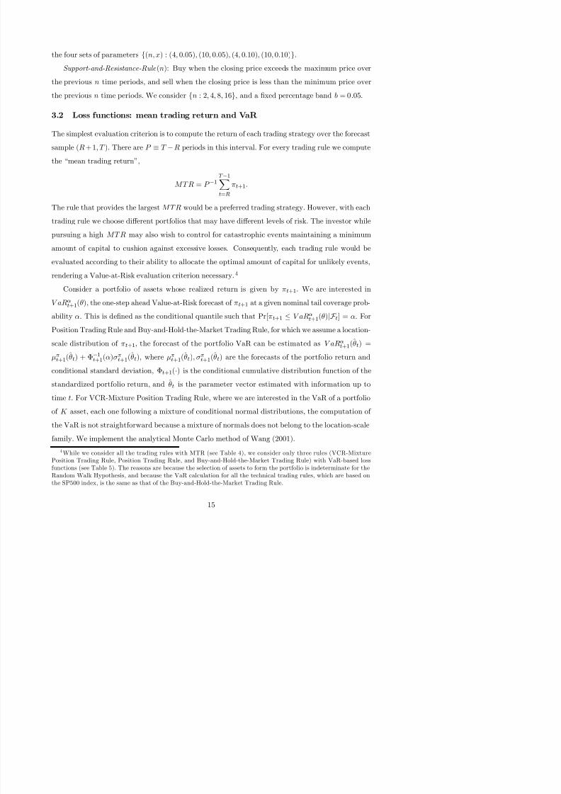
the four sets of parameters (n, x) : (4, 0.05), (10, 0.05), (4, 0.10), (10, 0.10).

Support-and-Resistance-Rule (n): Buy when the closing price exceeds the maximum price over

the previous n time periods, and sell when the closing price is less than the minimum price over

the previous n time periods. We consider n : 2, 4, 8, 16, and a fixed percentage band b = 0.05.

3.2 Loss functions: mean trading return and VaR

The simplest evaluation criterion is to compute the return of each trading strategy over the forecast

sample (R + 1, T ). There are P ≡ T −R periods in this interval. For every trading rule we compute

the “mean trading return”,

M T R = P −1T −1Xt=R

πt+1.

The rule that provides the largest M T R would be a preferred trading strategy. However, with each

trading rule we choose diff erent portfolios that may have diff erent levels of risk. The investor while

pursuing a high MT R may also wish to control for catastrophic events maintaining a minimum

amount of capital to cushion against excessive losses. Consequently, each trading rule would be

evaluated according to their ability to allocate the optimal amount of capital for unlikely events,

rendering a Value-at-Risk evaluation criterion necessary.4

Consider a portfolio of assets whose realized return is given by πt+1. We are interested in

V aRα

t+1(θ), the one-step ahead Value-at-Risk forecast of πt+1 at a given nominal tail coverage prob-

ability α. This is defined as the conditional quantile such that Pr[πt+1 ≤ V aRα

t+1(θ)|F t] = α. For

Position Trading Rule and Buy-and-Hold-the-Market Trading Rule, for which we assume a location-

scale distribution of πt+1, the forecast of the portfolio VaR can be estimated as V aRα

t+1(θt) =

µπt+1(θt) + Φ−1t+1(α)σπt+1(θt), where µπt+1(θt),σπt+1(θt) are the forecasts of the portfolio return and

conditional standard deviation, Φt+1(·) is the conditional cumulative distribution function of the

standardized portfolio return, and θt is the parameter vector estimated with information up to

time t. For VCR-Mixture Position Trading Rule, where we are interested in the VaR of a portfolio

of K asset, each one following a mixture of conditional normal distributions, the computation of



We evaluate the trading rules according to three VaR-based loss functions. The first loss function

aims to minimize the amount of capital to put aside (that is required to protect the investor against

a large negative return), the second loss function assesses which trading rule provides the correct

predicted tail coverage probability, and the third loss function is based on quantile estimation and

it evaluates which trading rule provides the best estimate of the VaR.

The first loss function V 1 sets the mean predicted “minimum required capital”, M RC αt+1(θt),

V 1 ≡ P −1

T −1Xt=R

M RC α

t+1(θt) ' P −1

T −1Xt=R

V aRα

t+1(θt).

A formula for MRC α as a function of V aRα with α = 0.01 is set by the Bassel Accord. See Jorion

(2000, p. 65). We approximate the formula by setting M RC α ' V aRα. Over the forecast period,

the trading rule that provides the lowest amount of capital to put aside will be preferred.

The second loss function V 2 aims to choose the trading rule that minimizes the diff erence between

the nominal and the empirical lower tail probability. It is an out-of-sample evaluation criterion

based on the likelihood ratio statistic of Christoff ersen (1998). Over the forecast interval (R +1, T ),

consider the following counts n1 =PT −1

t=R 1(πt+1 < V aRα

t+1(θt)) and n0 = P − n1. If the V aRα has

been correctly forecasted, n0 must be P × (1 − α) and n1 equals to P × α. In fact, the predictive

likelihood function of α given a sample

n1(πt+1 < V aRα

t+1(θt))

oT −1

t=Ris L(α) = (1 − α)n0αn1 and

the maximum likelihood estimator of α is α = n1/P. If we were to test for the null hypothesis thatE [1(πt+1 ≤ V aRα

t+1(θt))] = α, the likelihood ratio test 2(log L(α) − log L (α)) would be a suitable

statistic. The loss function V 2 is based on this statistic, and it is a distance measure between α and

α. A trading rule that minimizes V 2 will be preferred.

V 2 ≡ P −1 [2 log L(α) − 2log L (α)]

= P −1T −1Xt=R

2·1(πt+1 < V aRα

t+1(θt))log αα

+ 1(πt+1 > V aRα

t+1(θt)) log 1 − α1 − α

¸.

The third loss function V 3 chooses the trading rule that minimizes the objective function used

in quantile estimation (Koenker and Bassett, 1978)



3.3 Reality check

The question of interest is, among the twenty trading rules, which one is the best? Each ruleproduces diff erent forecasts that are evaluated according to the four loss functions introduced in

the previous subsection: −M TR , V 1, V 2, and V 3.5 The best trading rule is the one that provides

the minimum loss. However, for every loss function, how can we tell when the diff erence among

the losses produced by each trading rule is statistically significant? Furthermore, is a pairwise

comparison among the trading rules sufficient? Note that all trading rules are based on the same

data, and that their forecasts are not independent. We need a statistical procedure to assess whether

the diff erence among the losses is significant while, at the same time, taking into account any forecast

dependence across trading rules and controlling for potential biases due to data snooping. This

procedure is the “reality check” proposed by White (2000). Suppose that we choose one of the

trading rules as a benchmark. We aim to compare the loss of the remaining trading rules to that

of the benchmark. We formulate a null hypothesis that the trading rule with the smallest loss is no

better than the benchmark rule. If we reject the null hypothesis, there is at least one competing

trading rule that produces smaller loss than the benchmark. A brief sketch of the formal testing

procedure follows.

Let l be the number of competing trading rules (k = 1, . . . , l) to compare with the benchmark

rule (indexed as k = 0). For each trading rule k, one-step predictions are to be made for P periodsfrom R + 1 through T using a rolling sample, as explained in the previous sections. Consider a

generic loss function L(Y, θ) where Y consists of variables in the information set. In our case, we

have four loss functions: −M TR , V 1, V 2, and V 3. The best trading rule is the one that minimizes

the expected loss. We test a hypothesis about an l × 1 vector of moments, E (f ), where f ≡ f (Y, θ)

is an l × 1 vector with the kth element f k = L0(Y, θ)

−Lk(Y, θ), θ

≡plim θT , and L0(·, ·) is the

loss under the benchmark rule, Lk(·, ·) is the loss provided by the kth trading rule. A test for a

hypothesis on E (f ) may be based on the l×1 statistic f ≡ P −1PT −1

t=R f t+1, where f t+1 ≡ f (Y t+1, θt).

Our interest is to compare all the trading rules with a benchmark. An appropriate null hypoth-

esis is that all the trading rules are no better than a benchmark, i.e., H0 : max1≤k≤l E (f k) ≤ 0. This



is positive. Suppose that√

P (f − E (f ))d→ N (0,Ω) as P (T ) → ∞ when T → ∞, for Ω positive

semi-definite. White’s (2000) test statistic for H0 is formed as V ≡

max1≤k≤l√

P f k, which con-

verges in distribution to max1≤k≤lGk under H0, where the limit random vector G = (G1, . . . , Gl)0

is N (0,Ω). However, as the null limiting distribution of max1≤k≤lGk is unknown, White (2000,

Theorem 2.3) shows that the distribution of √

P (f ∗ − f ) converges to that of √

P (f − E (f )), where

f ∗ is obtained from the stationary bootstrap of Politis and Romano (1994). By the continuous

mapping theorem this result extends to the maximal element of the vector√

P (f ∗ − f ) so that the

empirical distribution of V ∗ = max1≤k≤l √ P (f ∗k − f k) is used to compute the p-value of V (White,

2000, Corollary 2.4). This p-value is called the “Reality Check p-value”.

3.4 Evaluation of trading rules

The out-of-sample performance of the aforementioned trading rules is provided in Tables 4 and

5. In Table 4, the trading rules are evaluated according to the MT R function, and in Table 5

according to the three VaR-based loss functions. In both cases, the in-sample size for the rolling

estimation is R = 300, and the out-of-sample forecast horizon is P = 299. The stationary bootstrap

(with smoothing parameter 0.25,which corresponds to the mean block length of 4) is implemented

with 1000 bootstrap resamples.6 In the first column of each table, we report the benchmark trading

rule to which the remaining rules will be compared.


In Table 4, we report the value of MTR function for each trading strategy. The VCR-Mixture

Position Trading Rule produces a mean trading return of 0.264 that is twice as much as the next

most favorable rule, which is the Position Trading Rule. This one and the Buy-and-Hold-the-

Market Rule produce similar results. We also find that all the technical trading rules are clearly

dominated by the VCR-Mixture Position rule, even though some of the Filter Rules and one of

the Support-and-Resistance Rule produce similar mean trading returns to those of the Position

Trading Rule and the Buy-and-Hold-the-Market Trading Rule. The statistical diff erence among



Following upon some of the criticisms of the profitability of momentum strategies, the superior

MTR of the VCR-Mixture Position Trading Rule may be the result of forming portfolios that are

very risky and consequently, the profits we observe are just due to a compensation for risk. We

have calculated the beta of each stock through a CAPM-type time series regression and, over each

period of the forecasting interval (299 periods), we have computed the average beta of the selected

portfolio of winner stocks. Since we are dealing with SP500 companies, the average beta of the

stocks in the index is about one but there are stocks with betas as high as 4.9. For the winner

portfolio, in one-third of the forecasting periods, the average beta is less than 1.1; in half of the

periods, the average beta is less than 1.4; and in about one-third of the periods is greater than 1.8.

Hence, the VCR-Mixture Position Trading Rule tends to pick up stocks over the full spectrum of

risk. As for the industrial nature of the five winner stocks that form the portfolio, we find that

the Information Technology sector (the riskiest according to the VCR model) is chosen 16% of the

time and the Utilities sector (the least risky) is chosen 10% of the time.

7

Thus, if our strategy werebased solely on the choice of risky asset, we would have expected to choose Information Technology

stocks more frequently.


In Table 5, we report the out-of-sample performance of the three trading rules evaluated ac-

cording to the loss functions V 1, V 2, and V 3, for two tail nominal probabilities α = 1% and α = 5%.

The results for α = 1% and 5% are virtually identical for all the three loss functions. With respect

to V 1, the Position Trading Rule seems to dominate statistically the remaining two rules providing

the least amount of required capital. However, when we consider V 2, the same rule performs very

poorly because it estimates the tail coverage rate of 7.2% at a nominal rate of 1%, and 14.0% at a

nominal rate of 5%. Thus, the smallest MRC of the Position Trading Rule comes at the expense

of a high tail failure rate. The VCR-Mixture Position Trading Rule delivers the best tail coverage,

estimating a tail coverage probability of 1.3% at a nominal rate of 1% and 4.3% at a nominal rate

of 5%. The White p-value confirms that this is the dominant rule in V 2. With respect to the loss



In addition to the four loss functions reported in Tables 4 and 5, we have also computed the

mean squared forecast errors (MSFE) of the returns, P −1PT −1t=R M −1PM

i=1(yi,t+1−

yi,t+1)2, and the

MSFE of the cross-sectional positions, P −1PT −1

t=R M −1PM

i=1(zi,t+1−zi,t+1)2. Based on these MSFE

losses, we compare the VCR-Mixture Position Trading Rule and the Position Trading Rule. With

the Position Trading Rule as the benchmark, the reality check p-values for both of the MSFE loss

functions are 0.000, clearly indicating that the VCR-Mixture Position Trading Rule is better than

the Position Trading Rule and thus underlying the importance of nonlinearity in the conditional

mean of the return process due to the VCR-weighted mixture.

4 Conclusions

Uncertainty, risk, and volatility aim to describe random events faced by economic agents, to which

we attach a probability of occurrence. Within this general context, we have added a new perspective

to the meaning of volatility. We have departed from the more classical meaning of volatility,

measured by a variance (or any other measure of dispersion), and we have added an ordinal measure,

the cross-sectional position of an asset return in relation to its peers. The meaning of volatility

that we put forward is a combination of a time-varying variance and a time-varying probability

of jumping positions in the cross-sectional return distribution of the assets that constitute the

market. The latter conveys a notion of interdependence among assets, implicitly revealing market

information, and in this sense, it has a multivariate flavor. Our task has been to investigate the

relevance of this approach.

For individual assets, we have modelled the joint dynamics of the cross-sectional position and

the asset return by analyzing (1) the marginal probability distribution of a sharp jump in the cross-

sectional position, and (2) the probability distribution of the asset return conditional on a jump.

The former is conducted within the context of a duration model, and the latter assumes that there

are diff erent dynamics in returns depending upon whether or not a jump has occurred. We have

estimated and tested the proposed models with weekly returns of those SP500 corporations that

have survived in the index from January 1, 1990 to August 31, 2001. The estimation results for the



probability of a sharp jump of 20-25%. Furthermore, we found that the expected return is a function

of past cross-sectional positions and that there are diff erent dynamics when the return is either at

extreme positions (top or bottom of the cross-sectional distribution) or at intermediate positions.

From an investor’s point of view, the most relevant question is how useful this model is. We

have designed an out-of-sample exercise where we have judged the adequacy of our model in two

dimensions: profitability and risk monitoring. Twenty diff erent trading rules, some model-based

and some technical rules, are compared within the statistical framework of White’s reality check,

which controls for potential biases due to data snooping. The VCR-Mixture Position Trading Rule

based on the one-step ahead forecast of our proposed model dominates all standard alternative

trading rules. It provides superior mean trading returns and accurate Value-at-Risk forecasts.

We summarize this research by underlining our main contribution. The conditional probability

of jumping cross-sectional positions is forecastable. This is possible because there is a persistence

on return performance. That is, assets that perform well (poorly) in the past, keep performing well(poorly) in the near future. We have called this probability Varying Cross-sectional Risk because

it provides an assessment of the chances of being a winner or a looser within the available set of

assets.



References

Aït-Sahalia, Yacine (2003), “Disentangling Diff

usion from Jumps”, forthcoming in the Journal of Financial Economics.

Christoff ersen, Peter F. (1998), “Evaluating Interval Forecasts,” International Economic Review ,

39, 841-862.

Engle, Robert F., David F. Hendry, and J.-F. Richard (1983), “Exogeneity”, Econometrica , 51,

277-304.

Engle, Robert F. and Jeff rey R. Russell (1998), “Autoregressive Conditional Duration: A NewModel for Irregularly Spaced Transaction Data,” Econometrica, 66, 1127-1162.

Granger, Clive W. J. (2002), “Some Comments on Risk”, Journal of Applied Econometrics , 17(5),

447-456.

Hamilton, James D. and Oscar Jordà (2002), “A Model of the Federal Funds Target,” Journal of

Political Economy, 110, 1135-1167.

Jegadeesh, Narasimhan and Sheridan Titman (1993), “Returns to Buying Winners and SellingLosers: Implications for Stock Market Efficiency”, Journal of Finance, 48, 65-91.

Jorion, Philippe (2000), Value at Risk , 2ed., McGraw-Hill.

Koenker, Roger and Gilbert Bassett, Jr. (1978), “Regression Quantiles”, Econometrica , 46(1),

33-50.

Lintner, John (1965), “The Valuation of Risky Assets and the Selection of Risky Investment in

Stock Portfolios and Capital Budget”, Review of Economics and Statistics, 47, 13-37.

Markowitz, Harry (1952), “Portfolio Selection”, Journal of Finance, 7, 77-99.

Politis, Dimitris N. and Joseph P. Romano (1994), “The Stationary Bootstrap”, Journal of Amer-

ican Statistical Association , 89, 1303-1313.

Sharpe, William (1964), “Capital Asset Prices: A Theory of Market Equilibrium under Conditions

of Risk”, Journal of Finance, 19, 425-442.Sullivan, Ryan, Allan Timmermann, and Halbert White (1999), “Data Snooping, Technical Trad-

ing Rule Performance, and the Bootstrap,” Journal of Finance , 54, 1647-1692.

Wang, Jin (2001), “Generating Daily Changes in Market Variables Using a Multivariate Mixture of

Normal Distributions”, Proceedings of the 2001 Winter Simulation Conference , B.A., Peters,



Table 1

Descriptive Statistics of Weekly Returns of the SP500 firms

January 1, 1990-August 31, 2001

Cross-sectional frequency distribution of unconditional moments

0

4

8

1216

20

24

28

32

36

-1.0 -0.5 0.0 0.5

Series: MEAN

Sample 1 343

Observations 343

Mean -0.007470

Median -0.016200

Maximum 0.771030

Minimum -0.964030

Std. Dev. 0.291280

Skewness -0.134563

Kurtosis 2.735350

Jarque-Bera 2.036118

Probability 0 .361296

0

10

20

30

40

50

60

70

2 4 6 8 10 12 14

Series: STD. DEVIATION

Sample 1 343

Observations 343

Mean 4.734877

Median 4.372920

Maximum 13.53324

Minimum 2.475010

Std. Dev. 1.583924

Skewness 1.911303

Kurtosis 8.657083


Probabil ity 0.000000

0

20

40

60

80

100

-2.5 0.0 2.5

Series: SKEWNESS

Sample 1 343

Observations 343

Mean -0.009417

Median 0.014850

Maximum 4.706040

Minimum -4.086720

Std. Dev. 0.681469

Skewness -0.173610

Kurtosis 17.02490

Jarque-Bera 2812.864Probability 0 .000000

240

280

320Series: KURTOSIS

Sample 1 343

Observations 343



Table 2

Cross-sectional frequency distribution of the estimates of the duration model

1411311211

'

1)(1)()(

1

1)1(1

)5.0(1)5.0(1

]'[)|1Pr(

−−−−−−

−−

−

−−−

+>+≤+=

+=+===

t t t t t t

t N t N t N

t t N t t t

z z y z y X

D

X F J p

δδδδδ

βψαψ

δψ

0

10

20

30

40

50

0.2 0.3 0.4 0.5 0.6

Series: ALPHA

Sample 1 343

Observations 343

Mean 0.371292

Median 0.364000

90% percentile 0.485000

Maximum 0.598000

Minimum 0.167000

Std. Dev. 0.081061

Skewness 0.309177

Kurtosis 2.814036


Probability 0.050823

0

20

40

60

80

100

120

140Series: BETA

Sample 1 343

Observations 343

Mean 0.098172

Median 0.056000


Maximum 0.724000

Minimum 0.010000

Std. Dev. 0.110893

Skewness 1.780148

Kurtosis 6.773379





0

10

20

30

40

50

60

0 2 4 6 8 10

Series: DELTA1

Sample 1 343

Observations 343

Mean 2.621921

Median 2.325000

90%percentile 4.757000

Maximum 10.23000

Minimum 0.008000Std. Dev. 1.580073

Skewness 1.480903

Kurtosis 6.378431



50

60

70Series: DELTA3

Sample 1 343

Observations 343

Mean -0.181584

Table 2 (cont.)

Cross-sectional frequency distribution of the estimates of the duration model

0

10

20

30

40

50

60

0.00 0.25 0.50 0.75 1.00 1.25

Series: DELTA2

Sample 1 343

Observations 343

Mean 0.218213

Median 0.146000


Maximum 1.369000

Minimum -0.027000Std. Dev. 0.223472

Skewness 1.804511

Kurtosis 7.277704





Table 2 (cont.)

Duration Model

Median parameter estimates for the industry sectors represented in the SP500 index

1411311211

'

1)(1)()(

1

1)1(1

)5.0(1)5.0(1

]'[)|1Pr(

−−−−−−

−−

−−−−

+>+≤+=

+=

+===

t t t t t t

t N t N t N

t t N t t t

z z y z y X

D

X F J p

δδδδδ

βψαψ

δψ

Sector % of firms βα ˆˆ + 2δ 3δ t p

Consumer Goods 28.3 0.455 0.162 -0.107 0.221

Energy 5.2 0.434 0.178 -0.198 0.239

Finance 12.5 0.457 0.221 -0.083 0.211

Health Care 7.0 0.444 0.103 -0.075 0.251

Industrials 12.8 0.455 0.193 -0.132 0.205

Information Technology 20.7 0.399 0.081 -0.056 0.301Material 6.7 0.484 0.120 -0.128 0.223

Utilities 6.7 0.548 0.214 -0.416 0.109

All sectors 100.0 0.455 0.146 -0.105 0.220



Table 3

Cross-sectional frequency distribution of the estimates

of the nonlinear model for expected returns

)1)(()(

0),(

1),();,|(

11,0111,111

12122

10100,0

11111,1

2

,,

2

,1,1

212

−−−−−−−

−−

−−

−−

−

−−+−=

++=

++=

++=

=

==

t t t t t t t

t t t

t t t

t t t

t t ot o

t t t

t t t

J y J ywith

z y

z y

J if N

J if N F J y f

µµε

τσρεωσ

ηγνµ

ηγνµ

σµ

σµθ

Conditional mean parameter estimates

0

5

10

15

20

25

-5.0 -2.5 0.0 2.5

Series: GAMMA1

Sample 1 343

Observations 343

Mean -1.137347

Median -1.114000

Maximum 2.809000

Minimum -6.194000

Std. Dev. 1.551645

Skewness -0.057839

Kurtosis 2.728742



4

8

12

16

20

24

28

32

-1.00 -0.75 -0.50 -0.25

Series: ETA1

Sample 1 343

Observations 343

Mean -0.606776

Median -0.609000

Maximum -0.227000

Minimum -1.030000

Std. Dev. 0.131909

Skewness 0.043542

Kurtosis 3.086106


Probability 0 .898370

30

40

50

60Series: GAMMA_0

Sample 1 343

Observations 343

Mean 0.108840

Median 0.149000

Maximum 4.394000

Minimum -6.06900020

30

40

50Series: ETA_0

Sample 1 343

Observations 343

Mean 0.373184

Median 0.370000

Maximum 1.305000

Minimum -0.071000

Std D 0 167893



Table 3 (cont.)

Conditional variance parameter estimates

0

4

8

12

16

20

24

28

0.0 0.5 1.0 1.5 2.0 2.5 3.0 3.5

Series: OMEGA

Sample 1 343

Observations 343

Mean 1.099802

Median 0.956000

Maximum 3.847000Minimum 0.072000

Std. Dev. 0.724246

Skewness 0.951112

Kurtosis 3.860637



0

20

40

60

80

100

120

0.0 0.1 0.2 0.3 0.4

Series: RHO

Sample 1 343

Observations 343

Mean 0.068586

Median 0.063000

Maximum 0.438000

Minimum 0.010000

Std. Dev. 0.043179

Skewness 2.707263Kurtosis 19.34593



30

40

50

60

70Series: TAU

Sample 1 343

Observations 343

Mean 0.825708

Median 0.866000

Maximum 0.980000

Minimum 0.126000

Std. Dev. 0.131893



Table 3 (cont.)

Expected Returns Model

Median parameter estimates for the industry sectors represented in the SP500 index

)1)(()(

0),(

1),();,|(

11,0111,111

12

122

10100,0

11111,1

2

,,

2

,1,1

212

−−−−−−−

−−

−−

−−

−

−−+−=

++=

++=

++=

=

==

t t t t t t t

t t t

t t t

t t t

t t ot o

t t t

t t t

J y J ywith

z y

z y

J if N

J if N F J y f

µµε

τσρεωσ

ηγνµ

ηγνµ

σµ

σµθ

Sector % of

firms1γ 0γ 1η 0η τρ ˆˆ +

Consumer Goods 28.3 -1.389 -0.073 -0.585 0.378 0.922

Energy 5.2 -1.025 0.145 -0.629 0.363 0.953

Finance 12.5 -0.660 0.519 -0.661 0.356 0.942

Health Care 7.0 -1.801 -0.121 -0.611 0.395 0.921

Industrials 12.8 -1.430 -0.166 -0.596 0.372 0.953

Information Technology 20.7 -1.405 0.196 -0.595 0.444 0.928

Material 6.7 -1.069 0.557 -0.601 0.349 0.921Utilities 6.7 0.116 0.987 -0.729 0.110 0.953

All sectors 100.0 -1.110 0.149 -0.609 0.370 0.930



Table 4

Out-of-sample evaluation of the trading rules

Loss function: Mean Trading Return

Benchmark trading rule MTR White p-value

VCR-Mixture Position Rule 0.264 1.000

Position Rule 0.131 0.079

Buy-and-Hold-the-Market Rule 0.115 0.072

Random Walk Hypothesis 0.000 0.000Filter-Rule (0.05) 0.062 0.008

Filter-Rule (0.10) 0.057 0.008

Filter-Rule (0.20) 0.119 0.077

Filter-Rule (0.50) 0.109 0.067

Moving-Average Rule (10, 2) 0.024 0.000

Moving-Average Rule (20, 2) -0.036 0.000

Moving-Average Rule (10, 4) 0.006 0.001Moving-Average Rule (20, 4) -0.009 0.000

Channel-Break-Out Rule (4, 0.05) 0.029 0.001


Channel-Break-Out Rule (4, 0.10) -0.006 0.000


Support-and-Resistance Rule (2) 0.124 0.040

Support-and-Resistance Rule (4) 0.006 0.000

Support-and-Resistance Rule (8) 0.040 0.000Support-and-Resistance Rule (16) 0.072 0.004

Notes: The mean trading return (MTR) represents the profit accrued from the respectivetrading rules. The out-of-sample horizon is P=299 and the in-sample horizon is R=300.

In each row, we present the trading rule selected as the benchmark with its correspondingMTR and the White reality check p-value for testing the null hypothesis that the

remaining trading rules are not any better than the benchmark rule. A large reality check p-value indicates that the null hypothesis cannot be rejected. For example, when theVCR-Mixture Position Rule is the benchmark, the reality check p-value 1.000 means that

this benchmark rule is not dominated by any of the other 19 alternative trading rules.



Table 5

Out-of-sample evaluation of the trading rules

Loss function: Value-at-Risk calculations

Panel 1. 01.0=α

Benchmark trading rule

V1 White p-value

V2 α White p-value

V3 White p-value

VCR-MixturePosition

1.952 0.000 0.007 0.013 1.000 0.025 0.996

Position 0.980 1.000 0.097 0.072 0.000 0.038 0.101

Buy-and-Hold-the-Market

2.351 0.000 0.040 0.029 0.000 0.040 0.042

Panel 2. 05.0=α

Benchmark

trading rule

V1 White

p-value

V2 α White

p-value

V3 White

p-value

VCR-Mixture

Position

1.395 0.000 0.019 0.043 1.000 0.073 0.998

Position 0.565 1.000 0.171 0.140 0.002 0.101 0.034

Buy-and-Hold-the-

Market

1.625 0.000 0.055 0.081 0.000 0.141 0.000

Notes: The out-of-sample period is P=299 and the in-sample period is R=300. V 1 , V 2 ,

and V 3 represent the values of the three VaR-based loss functions: MRC, coverage failure

rate, and goodness of fit in quantile estimation.α denotes the empirical failure rate at the

nominal rate α . The White reality check p-value corresponds to the test with a null

hypothesis that the remaining trading rules are not any better than the benchmark rule. Alarge reality check p-value indicates that the null hypothesis cannot be rejected. For

example, when the VCR-Mixture Position Trading Rule is the benchmark, the p-valuesare very large in terms of V 2 and V 3 , implying that this benchmark trading rule is not

dominated by the two alternative trading rules. In terms of V 1, the reality check p-value is0.0 and thus it is dominated by the alternative rules.



M

y y

z

M

j

t it j

t i

∑=

≤

=1

,,

,

)(111

1

1t

it

y

2t 3t 4t

R e t u r n s

Jump in ranking

No jump in ranking

Figure 1

Stylized description of the modelling problem

21

21

,,

,,

t it i

t it i

z z

y y

>

>

43

43

,,

,,

t it i

t it i

z z

y y

=

<

32

32

,,

,,

t it i

t it i

z z

y y

<

>

Cross-sectional histogramof realized returns (market)

jumps in rank and expected returns: introducing varying cross-sectional risk

Documents