Just Hire your Spouse: Empirical Evidence from a New Type of Political Favoritism Niklas Potrafke and Björn Kauder

Just hire your spouse:

Empirical evidence

from a new type of political favoritism

Björn Kauder1 ifo Institute

Niklas Potrafke2

University of Munich ifo Institute

8 April 2014

Abstract

We investigate a new type of political favoritism. Some members of the Bavarian parliament

hired relatives as office employees to be paid by taxpayers’ money. One of the best predictors

to favor relatives was being a member of parliament (MP) for few years and thus still having

outside options from politics. We investigate whether being involved in the scandal

influenced re-election prospects and voter turnout. The results do not show that being

involved in the scandal influenced the outcome and voter turnout of the 2013 state elections.

We propose three explanations: (i) the Bavarian state election was a test run of the German

federal election, (ii) the state government made a quite good job clarifying failings, (iii) in

June 2013, a tremendous flooding eclipsed the political scandal.

Keywords: political scandal, favoritism, re-election prospects, voter turnout

JEL Classification: D72

1 ifo Institute, Ifo Center for Public Finance and Political Economy, Poschingerstr.5, D-81679 Munich, Germany, Phone: + 49 89 9224 1331, Fax: + 49 89 907795 1331, E-mail: kauder@ifo.de 2 ifo Institute, Ifo Center for Public Finance and Political Economy, Poschingerstr.5, D-81679 Munich, Germany, Phone: + 49 89 9224 1319, Fax: + 49 89 907795 1319, E-mail: potrafke@ifo.de

2

1. Introduction

Political scandals often have extensive consequences. Scandals influence, for example,

politicians’ election prospects. When an incumbent experiences discredit, a pertinent question

is whether the incumbent will be re-elected. In a similar vein, challengers may not even have

a chance to become elected. Severe scandals bring individual political careers to an end.3

Political scandals have various facets: financial scandals include tax evasion, moral

scandals include sexual misconduct.4 Prominent examples of sexual misconduct are President

Bill Clinton’s affair with Monica Lewinsky and Dominique Strauss-Kahn’s sexual assault to a

cleaning lady. In 1998, Bill Clinton did not resign as president of the United States, and

because he was in his second term, did not need to fear his re-election. By contrast,

Dominique Strauss-Kahn’s political career abruptly ended. Strauss-Kahn was the managing

director of the International Monetary Fund and was expected to run as the presidential

candidate of the French Socialists having the best chances to win the 2011 French presidential

elections.

Experts examine political scandals and favoritism and elaborate on characteristics of

good and bad politicians.5 Good politicians have been described to be well educated and non-

corrupt. Good politicians are expected to be not involved in political scandals and favoritism.

When scandals occur, an issue is how politicians, especially party leaders or prime ministers,

deal with political scandals of their party or cabinet members (Dewan and Myatt 2007). When

a minister involved in a scandal heeds the call to resign, a government’s popularity may rise

(Dewan and Dowding 2005).6

In April 2013, Germany’s largest state Bavaria experienced a new political scandal

of favoritism. Members of the Bavarian parliament (Landtag) had hired relatives as office

3 In Japan, “the standard way of dealing with a scandal was to resign from the party and official posts but run again in the next elections“ (Nyblade and Reed 2008: 930). 4 Politicians either act corruptly for material gain or for electoral gain (Nyblade and Reed 2008). 5 In India, favoritism has been shown to improve economic outcomes in privileged electoral districts (Novosad and Asher 2013). 6 Doherty et al. (2011) examine scandalous behavior and the official’s responsibilities.

3

employees paid by the Bavarian parliament. The scandal became public because the expert in

German parliamentary affairs Hans Herbert von Arnim published a book elaborating on how

Bavarian politicians benefit from being in office (Arnim 2013). In 2000, the Bavarian

parliament tightened the state law. Members of the parliament were no longer allowed to hire

spouses, children, or parents as office employees.7 An interim arrangement allowed

employing relatives that had already assisted before the tightening of the law. But even 13

years after the interim arrangement was introduced, some MPs still employed close relatives.

Employing these relatives did not offend against the law but certainly smacked of exploiting

taxpayers’ money.

The state elections in Bavaria on 15 September 2013 and the German federal

elections on 22 September 2013 attached a great deal of importance to this scandal.

Politicians involved in the scandal realized the political hazard: some politicians who had

hired relatives repaid the relatives’ salaries immediately or donated the amounts. Some MPs

considered hiring relatives as legitimate in earlier times, but acknowledged that nowadays

MPs should not hire relatives. Although three parties are involved in the scandal, it is

conceivable that the reigning conservative Christian Social Union (CSU) incurred the largest

loss of votes. About 70% of the involved politicians are CSU members. The opposition

parties tried to exploit the scandal to increase their election prospects and replace the

predominant CSU-led state government.

The scandal in Bavaria has been a top issue in the German media for many weeks.8

We examine what determined the probability of having favored relatives and how the scandal

influenced the outcome and voter turnout of the 2013 state elections.

7 The law still allowed employing relatives other than spouses, children, and parents. In May 2013 the Bavarian parliament decided to also prohibit employing these relatives as of June 2013. 8 The media play a key role in (de)lighting political scandals. Ideologically biased media that favor the incumbent or challenger have incentives to hype or understate scandals.

4

2. Favoritism and scandals

Which incentives do MPs have to engage in favoritism? Politicians may view extracting rents

as justified from a public servants perspective. When a politician has served the state for a

long time it may give rise to a give-and-take perspective. This is all the more the case when

favoritism is common among MPs.9 Hiring relatives e.g. as office assistants is such a case of

favoritism.

Politicians and their assistants are likely to cooperate better when assistants are

acquaintances. Managers have been shown to favor employees that they personally know and

that these employees favor the manager in their decisions (Brandts and Solà 2010). Hiring

relatives is efficient when being relatives improves the collaboration. Hiring relatives is

favoritism when the collaboration does not improve. In Italy, public sector employees have

been shown to favor their children in gaining access to public sector positions (Scoppa

2009).10

In deciding on whether or not to engage in favoritism politicians consider the

probability of detection. When the media discovers a case of favoritism the political career

may end. The media or the party can force the politician to resign. It is also conceivable that

the political career ends because the politician is elected out of office. In Spain, incumbents

lost up to 14% of votes when incumbents have been accused with corruption and press

coverage has been substantial (Costas-Pérez et al. 2012).11 Scandals involving the incumbent

have also been shown to reduce trust in local politicians (Solé-Ollé and Sorribas-Navarro

2013). In Japan, candidates have been shown to have lost 1.34% of votes in the 1990 election

9 Gino et al. (2009) portray the nexus between an individual’s unethical behavior and unethical behavior of other individuals. 10 Prendergast and Topel (1996) examine how favoritism in firms influences employees’ compensation. Bramoullé and Goyal (2013) discuss the origins and consequences of favoritism. Parker (2005) investigates how reputational capital influences opportunistic behavior. 11 Puglisi and Snyder (2011) examine how newspapers‘ ideology influences media coverage of scandals in the United States. Bowler and Karp (2004) discuss how scandals influence the regard for political institutions.

5

because of scandals. In Great Britain, candidates have been shown to have lost 1.14% of votes

in the 1997 election because of scandals (Reed 1999).

Politicians’ opportunity costs are likely to influence politicians’ decisions to hire

relatives. Politicians who have been enrolled in politics for a long time face different

incentives as compared to politicians who just started their career. Politicians who just started

their political career still have outside options on the labor market. Consequently, for

politicians who just started their career extracting rents is a barely risky way to increase

income. By contrast, politicians who have been enrolled in politics for a long time hardly

have outside options on the labor market and experience a higher risk to hire relatives: when

the affair leaks out, the politician likely has to retire. We therefore expect politicians who

have been enrolled in politics for a long time to hire relatives to a lesser extent. We also

expect politicians in leading positions to hire relatives to a lesser extent, because politicians in

leading positions have more to lose. Learning effects are also likely to influence hiring

decisions: experienced politicians may understand better the risks associated with favoritism.

How politicians’ characteristics influence hiring relatives and how voters punish politicians

affected by the scandal remains as an empirical question.

3. Institutional background

3.1 The Bavarian political party landscape

The conservative CSU has dominated politics in Bavaria for decades.12 The leftist Social

Democratic Party (SPD) did not play an important role in Bavaria. All state prime ministers –

except one SPD prime minister between 1954 and 1957 – were members of the CSU.

The much smaller Free Democratic Party (FDP) formed a coalition with the CSU in

the 2008-2013 legislative period. Before 2008 the CSU was in power without any coalition

12 In other German states the conservatives are not represented by the CSU but by their sister party, the Christian Democratic Union (CDU). No party competition emerges between the CDU and the CSU and they form one faction in the federal parliament.

6

partner for 42 years. Figure 1 portrays the predominant role of the CSU in Bavarian state

elections. Only before 1966 the CSU formed coalitions with partners such as the SPD and the

FDP. Since 1986 the Greens (Bündnis 90/Die Grünen) and since 2008 the Free Voters (Freie

Wähler) are represented in the parliament. The vote share of the Greens never exceeded 10%.

The vote share of the Free Voters hardly exceeded 10%.

3.2 Bavarian state elections

In Bavarian state elections voters cast two votes in a personalized proportional representation

system. The first vote determines which candidate obtains the direct mandate in one of the 90

electoral districts with bare majority. The second vote sorts politicians on their party lists. The

first and second votes determine how many seats the individual parties receive in parliament.

Each party that received at least 5% of the first and second votes obtains a number of the 180

seats in the parliament according to the party’s first and second vote share. Candidates voted

into the parliament with the first vote (direct mandate) obtain their seats first. Candidates from

party lists obtain the remaining seats. When the number of direct mandates exceeds the

party’s vote share in a region, the party obtains excess mandates, and the other parties obtain

equalizing mandates.

4. Good and bad politicians: empirical analysis

4.1 MPs hiring relatives

The Bavarian president of parliament, Barbara Stamm, published a list including the MPs that

have employed spouses, children, or parents within the 2008-2013 and the two preceding

legislative periods (Stamm list, published on 3 May 2013). The list includes 79 (out of 360)

MPs from the 2008-2013 and the two preceding legislative periods. Three politicians from

this list have died in between, 54 are members of the reigning Christian Social Union (CSU),

20 are members of the Social Democratic Party (SPD), one is a member of the Greens

7

(Bündnis 90/Die Grünen), and one left the Greens to become an independent MP.13 MPs from

the 2008-2013 coalition partner of the CSU, the Free Democratic Party (FDP), and MPs from

the Free Voters (Freie Wähler) were not affected by the scandal. 17 politicians from the

Stamm list were still MPs in the 2008-2013 legislative period (all CSU members); three of

them were even ministers in the 2008-2013 government. The SPD and Greens politicians

from the Stamm list left the parliament at the latest in 2008. 16 of the MPs involved in the

scandal hired relatives only during the year 2000, shortly before the interim arrangement took

effect. It is conceivable that these MPs hired relatives though or because they knew that hiring

relatives was going to be forbidden. To be sure, some MPs also hired relatives other than

spouses, children, or parents. Hiring relatives other than spouses, children, or parents did not

violate the law. We do, however, not include relatives other than spouses, children, or parents

because MPs who hired them did not appear on the Stamm list; but these politicians were also

criticized in the public debate.

4.2 Descriptive statistics

We use data from the Centre of Bavarian History, the Bavarian Statistical Office, the

Bavarian parliament, and personal websites of the MPs. We only include those MPs in the

data set which were MPs at some time between 1998 (beginning of the Stamm list) and the

interim arrangement from December 2000 (see Section 1). It is not possible that MPs other

than from the time between 1998 and the interim arrangement from December 2000 were

included in the Stamm list. We therefore do not have MPs from the FDP and the Free Voters

in our data set, because the FDP and the Free Voters were not represented in the parliament

between 1998 and 2000. To be sure, we do not include politicians in the data set who became

MPs after the year 2000, as these MPs were not able to hire relatives according to the interim

13 We do not know the names of those three (CSU and SPD) MPs on the list that died in between. We therefore consider these MPs in the empirical analysis as not having hired relatives. We do not know the educational achievement of one SPD MP; because this MP hired a relative, the number of SPD MPs that hired relatives reduces to 19 in our data set.

8

arrangement. The sample thus reduces to 205 out of 360 MPs.14 Tables 1 and 2 show

descriptive statistics.

Figure 2 shows the shares of the parties’ MPs that employed relatives. The share of

CSU MPs that hired relatives (44%) is higher than the share of SPD MPs that hired relatives

(28%). The share of the Greens MPs that hired relatives is substantially smaller (8%). The

FDP and the Free Voters did not employ relatives. A t-test on means shows that there is a

significant difference between CSU and SPD politicians in hiring relatives. We reject the

hypothesis of no difference between CSU and SPD politicians with a t-value of 2.77.

4.3 Empirical strategy

The probit model has the following form:

Hired relativei = α + βYears MPi + Σj γj Personal characteristicsij + Σk δkPartyik

+ Σl εlRegionil+ ui

with i=1,…,205; j=1,…,8; k=1,2; l=1,…,6

where Hired relativei describes whether MP i has hired relatives and assumes the value one

when the MP i was on the Stamm list and zero otherwise. Years MPi describes the number of

years from MPs first election into parliament until the year 2000 (when an MP decided to hire

relatives). We include other control variables: Years in a partyi describes the number of years

since the MP’s beginning of membership in a political party until the year 2000.15 Agei

describes the age of the MP at the end of the year 2000. The dummy variable Femalei

14 The sample is larger than the regular number of MPs in the 1998-2003 legislative period because of successors of retired MPs. 15 We also consider membership in a youth organization of a political party as a membership in a political party. When an MP changed the party, we consider the beginning of membership in her/his first party.

9

assumes the value one for female MPs.16 Educationi describes the highest educational

achievement of an MP: the variable assumes the value one for having visited a school, the

value two for a completed vocational training (Berufsausbildung), the value three for a master

craftsman (Meister), the value four for a university of applied sciences degree

(Fachhochschulabschluss), the value five for a university degree, and the value six for a

PhD.17 The dummy variable Direct mandatei assumes the value one for MPs elected into the

parliament with the first vote in the 1998-2003 legislative period (see section 3.2). The

dummy variable Ministeri assumes the value one for MPs who were a minister at the end of

the year 2000. The dummy variable State secretaryi assumes the value one for MPs who were

a state secretary at the end of the year 2000. The dummy variable Leading party positioni

assumes the value one for MPs who were party leader or regional party leader in the end of

the year 2000.18 Partyik describes dummy variables for the CSU and the SPD (reference

category: Greens and independent MPs).19 Regionil describes dummy variables for the regions

where the individual MPs have been elected (reference category: Oberbayern), and ui

describes an error term. We estimate a probit model with standard errors robust to

heteroskedasticity (Huber/White/sandwich standard errors – see Huber 1967 and White

1980).

4.4 Regression results

Tables 3 and 4 show that the number of years being an MP influenced hiring relatives

(coefficient estimates in Table 3 and marginal effects in Table 4). The estimate in column (1)

of Table 4 indicates that a politician who was in the Bavarian parliament for a long time had a

16 Geys and Mause (in press) describe to which extent male and female legislators differ. 17 Our coding thus assumes a linear relation between the educational achievements. For parsimony reasons we do not include dummy variables for each educational achievement in the baseline model. 18 We do not include regional party leaders of the Greens because the Greens did not provide complete data on regional party leaders in 2000 upon request. 19 When an MP changed the party or became an independent MP, all dummy variables assume the value zero. There are two independent MPs in our data set.

10

lower probability of hiring relatives. The effect is statistically significant at the 10% level.

The numerical meaning of the effect is that one additional year in parliament decreased the

probability of hiring relatives by 1.0 percentage points. When the years in parliament variable

increased by one standard deviation (somewhat more than seven years), the probability of

hiring relatives decreased by about 7.2 percentage points. The years since the beginning of

membership in a political party negatively influenced the probability of hiring relatives. The

effect is statistically significant at the 10% level. One additional year since the beginning of

membership in a political party decreased the probability of hiring relatives by 1.0 percentage

points. Older MPs were more likely to hire relatives. The effect is statistically significant at

the 1% level. The numerical meaning of the effect is that being one year older increased the

probability of hiring relatives by 1.3 percentage points. The effects of years in parliament,

years in a party, and age indicate that politicians were likely to hire relatives when they had

little experience in the political business and when they were of higher age (lateral entrants);

young career politicians were, by contrast, less likely to hire relatives. Being a female MP and

the level of education do not turn out to be statistically significant at conventional levels. Also

being elected into parliament with the first vote (direct mandate), being a minister, and being

a state secretary does not turn out to be statistically significant. Holding a leading party

position decreased the probability of hiring relatives. The effect is statistically significant at

the 5% level. The numerical meaning of the effect is that being party leader or regional party

leader decreased the probability of hiring relatives by 34.0 percentage points. CSU

membership increased the probability of hiring relatives. The effect is statistically significant

at the 5% level. The numerical meaning of the effect is that being a CSU member increased

the probability of hiring relatives by 32.5 percentage points as compared with the Greens and

independent MPs (reference category). SPD membership does not turn out to be statistically

significant. The electoral districts also influenced the probability of hiring relatives. The

probability of hiring relatives was lowest in Oberbayern (reference category); the probability

11

was highest in Schwaben and Unterfranken. The effects are statistically significant at the 1%

level. Being a politician from Schwaben or Unterfranken increased the probability of hiring

relatives by 43.0 percentage points and 37.2 percentage points. The probability of hiring

relatives was also higher in the Oberpfalz and Oberfranken. The effects are statistically

significant at the 5% level. The numerical meaning of the effects is that being a politician

from the Oberpfalz or Oberfranken increased the probability of hiring relatives by about 26

percentage points. The effects of Niederbayern and Mittelfranken lack statistical significance

at conventional levels.

Column (2) includes MPs that have not reported when they became a party member.

Including MPs that have not reported when they became a party member allows examining all

205 observations in the data set. The estimate again indicates that a politician who has been in

the Bavarian parliament for a long time had a lower probability of hiring relatives. The effect

is statistically significant at the 10% level. The numerical meaning of the effect is that one

additional year in parliament decreased the probability of hiring relatives by 0.9 percentage

points. Older MPs were again more likely to hire relatives. The effect is statistically

significant at the 10% level. Being one year older increased the probability of hiring relatives

by 0.7 percentage points. Being a female MP, the level of education, and whether the MP

obtained a direct mandate lacks statistical significance. Also being a minister and being a state

secretary does not turn out to be statistically significant at conventional levels. Holding a

leading party position decreased the probability of hiring relatives. The effect is statistically

significant at the 5% level. The numerical meaning of the effect is that being party leader or

regional party leader decreased the probability of hiring relatives by 36.3 percentage points.

CSU membership positively influenced the probability of hiring relatives. The effect is

statistically significant at the 5% level. The numerical meaning of the effect is that being a

CSU member increased the probability of hiring relatives by 30.1 percentage points as

compared with the Greens and independent MPs (reference category). SPD membership does

12

not turn out to be statistically significant. Inferences of the electoral district variables do not

change as compared with column (1).

4.5 Robustness tests

We tested whether the results are driven by including/excluding those MPs who hired

relatives in the year 2000. In the sample with 178 observations, excluding the MPs who hired

relatives in the year 2000 renders the years in a party variable and the CSU variable to lack

statistical significance (replicating column (1) of Table 4). In the sample with 205

observations, excluding the MPs who hired relatives in the year 2000 renders the years MP

variable and the CSU variable to lack statistical significance. The female variable is, however,

statistically significant (replicating column (2) of Table 4).

It is conceivable that re-election prospects influenced whether an MP hired relatives.

An MP may well expect her/his re-election when the vote margin in the last election was

large.20 Controlling for the 1998 vote margin reduces, however, the sample size to 85 and

104, because controlling for vote margin includes only MPs elected as direct candidates (see

Section 3.2). The vote margin variable does not turn out to be statistically significant. When

the vote margin variable is included, the effects of years MP, years in a party, age, and

leading party position lack statistical significance. We reran our baseline model with the

subsample for which the vote margin variable is available: the effects of years MP, years in a

party, age, and leading party position lack statistical significance. Inferences thus change

when we reduce the sample from 205 to 104 or from 178 to 85 observations.

20 Geys (2013) discusses how election cycles influence outside activities of MPs in the UK and shows a particularly strong election effect for MPs in marginal seats.

13

5. Election effects: empirical analysis

5.1 Vote shares and voter turnout

The conservative CSU won the state elections on 15 September 2013 and received 48% of the

votes. As in the 2008 election, the CSU won all districts except one in the 2013 election. We

examine how the scandal influenced the vote share of the CSU by comparing every individual

district in the elections 2008 and 2013. As the SPD and Greens MPs who hired relatives left

the parliament at the latest in 2008, we consider no other party than the CSU when we

examine how the scandal influenced the election outcome. We directly investigate how the

scandal influenced a politician’s re-election when the individual politician ran for office again

after she/he experienced the scandal.21 When the scandal brought a politician’s career to an

end, or a politician would have ended her/his career in any event – the scandal

notwithstanding – we cannot compare the individual vote of the elections in 2008 and 2013.

We thus also compare the vote share of the CSU in districts affected by the scandal with the

vote share of the CSU in districts not affected by the scandal, independent of the party’s

candidate. It is conceivable that the scandal also influenced voter turnout as a result of

disenchantment with politics. We therefore examine how the scandal influenced voter turnout

by comparing the elections 2008 and 2013 in every individual district.

5.2 Descriptive statistics

We use data from the Centre of Bavarian History, the Bavarian Statistical Office, the

Bavarian parliament, and personal websites of the MPs. We only include those (73 out of 91)

districts that have not been adjusted between the 2008 and the 2013 state elections. Tables 5

and 6 show descriptive statistics. The samples include 88 and 146 observations.

21 In districts that were not adjusted between the 2008 and the 2013 state elections, 50% of the MPs who hired relatives and 63% of the MPs who did not hire relatives stood for re-election. A t-test on means shows that there is no significant difference between MPs who hired relatives and MPs who did not hire relatives in the decision to stand for re-election. We do not reject the null hypothesis of no difference between MPs who hired relatives and MPs who did not hire relatives with a t-value of 0.94.

14

Figure 3 shows polls for the 2008-2013 legislative period. The scandal arose in

April/May 2013 and as Figure 3 shows CSU vote intentions declined from about 49% to

about 46% in April/May 2013. The CSU recovered slowly from the scandal. The CSU vote

share was 47% and 48% in July and August 2013. Figure 4 shows the first vote share of the

CSU in the state elections 2008 and 2013, for districts being and not being affected by the

scandal. The CSU first vote share increased from 45% to 49% in scandal districts and from

43% to 47% in other districts. A t-test on means shows that there is no significant difference

between scandal districts and other districts in the CSU first vote share change. We do not

reject the null hypothesis of no difference between scandal districts and other districts with a

t-value of 0.42. Figure 5 shows the total vote share (sum of first and second votes) of the CSU

in the state elections 2008 and 2013, for districts being and not being affected by the scandal.

The CSU total vote share increased from 47% to 50% in scandal districts and from 44% to

48% in other districts. A t-test on means shows that there is no significant difference between

scandal districts and other districts in the CSU total vote share change. We do not reject the

null hypothesis of no difference between scandal districts and other districts with a t-value of

1.56. Figure 6 shows the voter turnout in the state elections 2008 and 2013, for districts being

and not being affected by the scandal. The voter turnout increased from 58% to 64% in both

scandal districts and other districts. A t-test on means shows that there is no significant

difference between scandal districts and other districts in the voter turnout change. We do not

reject the null hypothesis of no difference between scandal districts and other districts with a

t-value of 0.39.

15

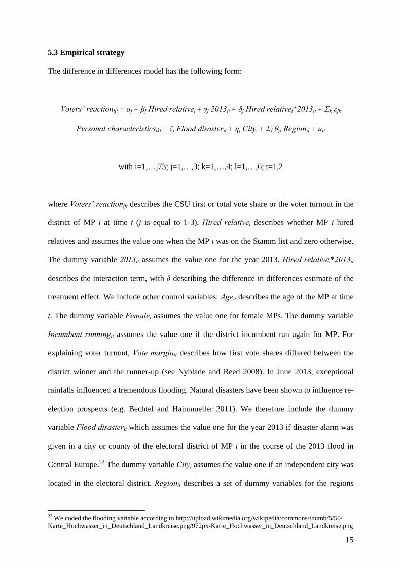
5.3 Empirical strategy

The difference in differences model has the following form:

Voters’ reactionijt = αj + βjHired relativei + γj 2013it + δj Hired relativei*2013it + Σk εjk

Personal characteristicsikt+ ζj Flood disasterit + ηj Cityi + Σl θjlRegionil + uit

with i=1,…,73; j=1,…,3; k=1,…,4; l=1,…,6; t=1,2

where Voters’ reactionijt describes the CSU first or total vote share or the voter turnout in the

district of MP i at time t (j is equal to 1-3). Hired relativei describes whether MP i hired

relatives and assumes the value one when the MP i was on the Stamm list and zero otherwise.

The dummy variable 2013it assumes the value one for the year 2013. Hired relativei*2013it

describes the interaction term, with δ describing the difference in differences estimate of the

treatment effect. We include other control variables: Ageit describes the age of the MP at time

t. The dummy variable Femalei assumes the value one for female MPs. The dummy variable

Incumbent runningit assumes the value one if the district incumbent ran again for MP. For

explaining voter turnout, Vote marginit describes how first vote shares differed between the

district winner and the runner-up (see Nyblade and Reed 2008). In June 2013, exceptional

rainfalls influenced a tremendous flooding. Natural disasters have been shown to influence re-

election prospects (e.g. Bechtel and Hainmueller 2011). We therefore include the dummy

variable Flood disasterit which assumes the value one for the year 2013 if disaster alarm was

given in a city or county of the electoral district of MP i in the course of the 2013 flood in

Central Europe.22 The dummy variable Cityi assumes the value one if an independent city was

located in the electoral district. Regionil describes a set of dummy variables for the regions

22 We coded the flooding variable according to http://upload.wikimedia.org/wikipedia/commons/thumb/5/50/ Karte_Hochwasser_in_Deutschland_Landkreise.png/972px-Karte_Hochwasser_in_Deutschland_Landkreise.png

16

where the individual MPs were elected (reference category: Oberbayern), and uit describes an

error term. We estimate a difference in differences model with standard errors robust to

heteroskedasticity (Huber/White/sandwich standard errors – see Huber 1967 and White

1980).

5.4 Regression results

The results in Table 7 do not show that the scandal influenced the CSU vote share as

measured by the 2013 and the 2008 state election results. The estimate in column (1) of Table

7 considers the CSU first vote results and thus only includes those MPs and MP candidates

that have been elected in 2008 (and re-elected in 2013) into parliament with the first vote. The

results do not indicate that the scandal was associated with the CSU share of first votes: the

interaction term between Hired relativei and 2013 does not turn out to be statistically

significant at conventional levels. The results do also not indicate a scandal district specific

effect (Hired relativei) or that the CSU first vote share was higher or lower in 2013. The age

of the MP or MP candidate, whether the MP or MP candidate is female, and whether the MP

or MP candidate is the incumbent do not turn out to be statistically significant.23 The CSU

first vote share increased when the district was affected by the 2013 flood disaster. The effect

is statistically significant at the 1% level. The numerical meaning of the effect is that when

the district was affected by the flood the CSU first vote share increased by 6.8 percentage

points. The magnitude of the effect resembles the 7 percentage points effect for the 2002 Elbe

flooding (Bechtel and Hainmueller 2011). The CSU first vote share decreased when an

electoral district included an independent city. The effect is statistically significant at the 1%

level. The numerical meaning of the effect is that the CSU first vote share decreased by 4.6

percentage points when an electoral district included an independent city. The electoral

23 To be sure, the incumbent variable assumes the value one for all MPs in the year 2013 because we include only MPs that have been elected in 2008 (and re-elected in 2013). The incumbent variable assumes, however, the value zero for the year 2008 when the MP candidate was not elected in the year 2003.

17

districts also influenced the CSU first vote share. The CSU first vote share was higher in the

Oberpfalz, Oberfranken, Unterfranken, and Schwaben as compared to Oberbayern (reference

category). The effects are statistically significant at the 1% level. The numerical meaning of

the effects is that the CSU obtained in the Oberpfalz 10.5 percentage points, in Oberfranken

6.3 percentage points, in Unterfranken 5.2 percentage points, and in Schwaben 3.9 percentage

points more first votes as compared to Oberbayern. The CSU first vote share was also higher

in Niederbayern. The effect is statistically significant at the 10% level. The numerical

meaning of the effect is that the CSU obtained in Niederbayern 3.3 percentage points more

first votes as compared to Oberbayern. The effect of Mittelfranken lacks statistical

significance at conventional levels.

The estimate in column (2) of Table 7 considers the CSU total vote results and

includes all electoral districts, also those where the MP candidate changed between 2008 and

2013. The results do not indicate that the scandal was associated with the CSU share of total

votes: the interaction term between Hired relative and 2013 does not turn out to be

statistically significant at conventional levels. The results do also not indicate a scandal

district specific effect (Hired relative). The CSU total vote share was higher in 2013. The

effect is statistically significant at the 1% level. The numerical meaning of the effect is that

the CSU total vote share increased by 2.9 percentage points as compared to 2008. The effects

of the age and gender of the MP or MP candidate and whether she/he was the incumbent lack

statistical significance. The CSU total vote share increased when the district was affected by

the 2013 flood disaster. The effect is statistically significant at the 1% level. The numerical

meaning of the effect is that when the district was affected by the flood the CSU total vote

share increased by 5.9 percentage points. The CSU total vote share decreases when an

electoral district includes an independent city. The effect is statistically significant at the 1%

level. The numerical meaning of the effect is that the CSU total vote share decreased by 5.2

percentage points when an electoral district included an independent city. The CSU total vote

18

share also differed across regions: The CSU total vote share was highest in Oberpfalz,

Unterfranken, and Schwaben. The effects are statistically significant at the 1% level. The

numerical meaning of the effects is that the CSU obtained in the Oberpfalz 7.5 percentage

points, in Unterfranken 6.0 percentage points, and in Schwaben 4.9 percentage points more

total votes as compared to Oberbayern (reference category). The CSU total vote share was

also higher in Oberfranken and Niederbayern. The effects are statistically significant at the

5% and 10% level. The numerical meaning of the effects is that the CSU obtained in

Oberfranken 3.8 percentage points and in Niederbayern 2.3 percentage points more total votes

as compared to Oberbayern. The effect of Mittelfranken lacks statistical significance at

conventional levels.

The estimate in column (1) of Table 8 considers voter turnout and includes all

electoral districts. The results do not indicate that the scandal was associated with voter

turnout: the interaction term between Hired relative and 2013 does not turn out to be

statistically significant at conventional levels. The scandal district specific effect (Hired

relative) does not turn out to be statistically significant. The results do, however, indicate that

voter turnout was higher in 2013. The effect is statistically significant at the 1% level. The

numerical meaning of the effect is that voter turnout increased by 6.2 percentage points as

compared to 2008. The effects of the age and gender of the MP or MP candidate, and whether

the MP or MP candidate was the incumbent lack statistical significance. The effect of the vote

margin between the winner and the runner-up of the district and the effect of the flood disaster

do also not turn out to be statistically significant at conventional levels. Voter turnout

decreased when an electoral district included an independent city. The effect is statistically

significant at the 1% level. The numerical meaning of the effect is that voter turnout

decreased by 3.1 percentage points when an electoral district included an independent city.

Voter turnout differed across the electoral districts and was highest in Oberbayern (reference

category); voter turnout was lower in Niederbayern, Schwaben, and Unterfranken. The effects

19

are statistically significant at the 1% level. In Niederbayern voter turnout was 6.1 percentage

points, in Schwaben 4.9 percentage points, and in Unterfranken 2.9 percentage points lower

as compared to Oberbayern. Voter turnout was also lower in Oberfranken. The effect is

statistically significant at the 10% level. The numerical meaning of the effect is that voter

turnout was 1.8 percentage points lower in Oberfranken as compared to Oberbayern. The

effects of the Oberpfalz and Mittelfranken do not turn out to be statistically significant at

conventional levels.

5.5 Robustness tests

We tested whether the scandal influenced the other parties’ vote shares. We replicated the

regressions described in Table 7 with the vote shares of the SPD, the Greens, the FDP, and the

Free Voters as dependent variable. The results do, however, not indicate that other parties

benefitted in districts where the CSU hired relatives.

We tested how MPs who hired relatives during the year 2000 influenced the CSU vote

share and voter turnout. We thus considered only those MPs who hired relatives during the

year 2000 as being affected by the scandal. The results do, however, not change as compared

to considering all MPs who hired relatives as being affected by the scandal (except the

Oberfranken dummy in the voter turnout regression). We also tested whether the results are

driven by including/excluding the MPs who hired relatives in the year 2000. Excluding the

MPs who hired relatives in the year 2000 in the CSU first vote share regression renders the

2013 variable to be statistically significant at the 10% level. Excluding the MPs who hired

relatives in the year 2000 in the voter turnout regression renders the flood disaster and the

Oberpfalz variables to be statistically significant at the 10% level.

20

6. Conclusion

The family scandal in Bavaria 2013 has been a prime example for favoritism in politics. One

of the best predictors to favor relatives was being an MP for few years. Politicians who have

been in the parliament for few years may still have outside options from politics and therefore

did not hazard their lifework by hiring relatives. By contrast, politicians who devoted their

lives to politics were more hesitant hiring relatives. One may well conclude that these results

provide evidence for too low salaries of MPs. Empirical evidence has shown that the political

entry decision of citizens depends on the opportunity costs (Caselli and Morelli 2004;

Messner and Polborn 2004), and that politicians’ performance depends on politicians’

remuneration (Besley 2004). In Finland, a wage increase has been shown to increase the share

of parliamentary candidates with higher education among female candidates, but not among

male candidates (Kotakorpi and Poutvaara 2011). In Italy, higher wages have been shown to

attract more educated mayor candidates, and that better paid politicians improve efficiency

(Gagliarducci and Nannicini 2013). Politicians with higher ex-ante quality, such as previous

market income, have been shown to be more likely to run in contestable districts (Galasso and

Nannicini 2011). In Germany, MPs have been shown to benefit from a wage gap of 35-65%

as compared to executives in the private sector; the calculation of the wage gap, however,

includes politicians’ outside earnings. The wage gap of politicians has been shown to be zero

as compared with top level executives in the private sector (Peichl et al. 2013). The frequent

use of secondary income opportunities by MPs supports our interpretation of too low salaries

of MPs.24

The results do not show that the scandal influenced the election outcome and voter

turnout. Three explanations spring to mind why being involved in the scandal did not

influence re-election prospects and voter turnout. First, the Bavarian state election on 15

24 For a survey on moonlighting by politicians see Geys and Mause (2013). Gagliarducci et al. (2010) examine the relation between politicians’ ability, income from the private sector, and commitment among members of the Italian parliament. Besley and Larcinese (2011) discuss the determinants of UK MPs’ expense claims.

21

September 2013 was a test run of the German federal election on 22 September 2013. State

elections induce signaling effects for the federal elections. Because the Bavarian electorate

has more conservative views than the average German electorate, Bavarian voters wanted to

give the CDU/CSU encouragement and prevent a left-wing federal government. Second, the

conservative Bavarian government made a quite good job dealing with the scandal and

clarifying failings. The conservative faction leader immediately resigned. The conservative

president of parliament compiled a list of all MPs involved in the scandal. Many MPs repaid

the relatives’ salaries. Third, in June 2013, exceptional rainfalls influenced a tremendous

flooding. The state government again proved competent crisis management. The natural

disaster eclipsed the political scandal.

22

References

Arnim, Hans Herbert von (2013), Die Selbstbediener: Wie bayerische Politiker sich den Staat

zur Beute machen, Heyne Verlag, München.

Bechtel, Michael M. and Jens Hainmueller (2011), How lasting is voter gratitude? An

analysis of the short- and long-term electoral returns to beneficial policy, American

Journal of Political Science 55, 851-867.

Besley, Timothy (2004), Paying politicians: Theory and evidence, Journal of the European

Economic Association 2, 193-215.

Besley, Timothy and Valentino Larcinese (2011), Working or shirking? Expenses and

attendance in the UK parliament, Public Choice 146, 291-317.

Bowler, Shaun and Jeffrey A. Karp (2004), Politicians, scandals, and trust in government,

Political Behavior 26, 271-287.

Bramoullé, Yann and Sanjeev Goyal (2013), Favoritism, mimeo.

Brandts, Jordi and Carles Solà (2010), Personal relations and their effect on behavior in an

organizational setting: An experimental study, Journal of Economic Behavior &

Organization 73, 246-253.

Caselli, Francesco and Massimo Morelli (2004), Bad politicians, Journal of Public Economics

88, 759-782.

Costas-Pérez, Elena, Albert Solé-Ollé and Pilar Sorribas-Navarro (2012), Corruption

scandals, voter information, and accountability, European Journal of Political

Economy 28, 469-484.

Dewan, Torun and Keith Dowding (2005), The corrective effect of ministerial resignations on

government popularity, American Journal of Political Science 49, 46-56.

Dewan, Torun and David P. Myatt (2007), Scandal, protection, and recovery in the cabinet,

American Political Science Review 101, 63-77.

Doherty, David, Conor M. Dowling and Michael G. Miller (2011), Are financial or moral

scandals worse? It depends, Political Science & Politics 44, 749-757.

Gagliarducci, Stefano and Tommaso Nannicini (2013), Do better paid politicians perform

better? Disentangling incentives from selection, Journal of the European Economic

Association 11, 369-398.

Gagliarducci, Stefano, Tommaso Nannicini and Paolo Naticchioni (2010), Moonlighting

politicians, Journal of Public Economics 94, 688-699.

Galasso, Vincenzo and Tommaso Nannicini (2011), Competing on good politicians,

American Political Science Review 105, 79-99.

23

Geys, Benny (2013), Election cycles in MPs’ outside interests? The UK house of commons,

2005-2010, Political Studies 61, 462-472.

Geys, Benny and Karsten Mause (2013), Moonlighting politicians: A survey and research

agenda, Journal of Legislative Studies 19, 76-97.

Geys, Benny and Karsten Mause (in press), Are female legislators different? Exploring sex

differences in German MPs' outside interests, Parliamentary Affairs.

Gino, Francesca, Shahar Ayal and Dan Ariely (2009), Contagion and differentiation in

unethical behavior – the effect of one bad apple on the barrel, Psychological Science

20, 393-398.

Huber, Peter J. (1967), The behavior of maximum likelihood estimates under nonstandard

conditions, Proceedings of the Fifth Berkeley Symposium on Mathematical Statistics

and Probability, 221-233.

Kotakorpi, Kaisa and Panu Poutvaara (2011), Pay for politicians and candidate selection: An

empirical analysis, Journal of Public Economics 95, 877-885.

Messner, Matthias and Mattias K. Polborn (2004), Paying politicians, Journal of Public

Economics 88, 2423-2445.

Novosad, Paul and Sam Asher (2013), Politics and local economic growth: Evidence from

India, mimeo.

Nyblade, Benjamin and Steven R. Reed (2008), Who cheats? Who loots? Political

competition and corruption in Japan, 1947-1993, American Journal of Political

Science 52, 926-941.

Parker, Glenn R. (2005), Reputational capital, opportunism, and self-policing in legislatures,

Public Choice 122, 333-354.

Peichl, Andreas, Nico Pestel and Sebastian Siegloch (2013), The politicians’ wage gap:

Insights from German members of parliament, Public Choice 156, 653-676.

Prendergast, Canice and Robert H. Topel (1996), Favoritism in organizations, Journal of

Political Economy 104, 958-978.

Puglisi, Riccardo and James M. Snyder, Jr. (2011), Newspaper coverage of political scandals,

Journal of Politics 73, 931-950.

Reed, Steven R. (1999), Punishing corruption: The response of the Japanese electorate to

scandals, in O. Feldman, ed., Political psychology in Japan: Behind the nails that

sometimes stick out (and get hammered down), Nova Science Publishers, Commack,

New York, 131-148.

24

Scoppa, Vincenzo (2009), Intergenerational transfers of public sector jobs: A shred of

evidence on nepotism, Public Choice 141, 167-188.

Solé-Ollé, Albert and Pilar Sorribas-Navarro (2013), Does exposure to corruption erode trust

in government? Evidence from a matched sample of local scandals in Spain, mimeo.

White, Halbert (1980), A heteroskedasticity-consistent covariance matrix estimator and a

direct test for heteroskedasticity, Econometrica 48, 817-838.

25

Figure 1: The CSU is the predominant party in Bavaria

Figure 2: Only MPs from CSU, SPD, and Greens hired relatives

Number of MPs that hired relatives: CSU: 54, SPD: 19, Greens: 1. T-test on means (difference between CSU and SPD) with t-value 2.77.

26

Figure 3: The CSU lost in polls after the scandal arose in April/May 2013

The last observation describes the 2013 state elections result. Figure 4: The CSU obtained more first votes in both scandal and other districts

Number of scandal districts: 8, number of other districts: 36. T-test on means (difference between scandal districts and other districts) with t-value 0.42.

27

Figure 5: The CSU obtained more total votes in both scandal and other districts

Number of scandal districts: 16, number of other districts: 57. T-test on means (difference between scandal districts and other districts) with t-value 1.56. Figure 6: Voter turnout increased in both scandal and other districts

Number of scandal districts: 16, number of other districts: 57. T-test on means (difference between scandal districts and other districts) with t-value 0.39.

28

Table 1: Descriptive statistics (hiring relatives; sample including Years in a party)

Obs. Mean Std. Dev. Min Max Hired relative 178 0.37 0.48 0 1Years MP 178 9.53 7.16 0 30Years in a party 178 26.91 8.09 3 45Age 178 51.90 7.85 29 65Female 178 0.25 0.44 0 1Education 178 3.96 1.56 1 6Direct mandate 178 0.48 0.50 0 1Vote margin 85 0.22 0.12 0.00 0.52Minister 178 0.05 0.22 0 1State secretary 178 0.04 0.19 0 1Leading party position 178 0.06 0.23 0 1CSU 178 0.57 0.50 0 1SPD 178 0.35 0.48 0 1Greens 178 0.07 0.25 0 1Niederbayern 178 0.08 0.27 0 1Oberbayern 178 0.35 0.48 0 1Oberpfalz 178 0.10 0.30 0 1Oberfranken 178 0.10 0.29 0 1Mittelfranken 178 0.13 0.34 0 1Unterfranken 178 0.10 0.30 0 1Schwaben 178 0.13 0.34 0 1

FDP and Free Voters are not in the data set, because their MPs did not hire relatives.

29

Table 2: Descriptive statistics (hiring relatives; sample excluding Years in a party)

Obs. Mean Std. Dev. Min Max Hired relative 205 0.37 0.48 0 1Years MP 205 10.32 7.64 0 30Age 205 52.55 8.07 29 69Female 205 0.22 0.42 0 1Education 205 4.00 1.56 1 6Direct mandate 205 0.51 0.50 0 1Vote margin 104 0.23 0.12 0.00 0.52Minister 205 0.05 0.23 0 1State secretary 205 0.03 0.18 0 1Leading party position 205 0.05 0.23 0 1CSU 205 0.60 0.49 0 1SPD 205 0.33 0.47 0 1Greens 205 0.06 0.24 0 1Niederbayern 205 0.10 0.30 0 1Oberbayern 205 0.33 0.47 0 1Oberpfalz 205 0.09 0.29 0 1Oberfranken 205 0.10 0.30 0 1Mittelfranken 205 0.14 0.34 0 1Unterfranken 205 0.11 0.32 0 1Schwaben 205 0.14 0.34 0 1

FDP and Free Voters are not in the data set, because their MPs did not hire relatives.

30

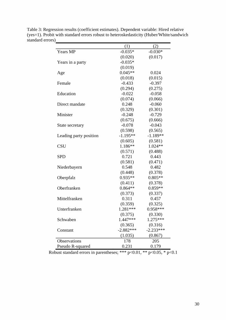
Table 3: Regression results (coefficient estimates). Dependent variable: Hired relative (yes=1). Probit with standard errors robust to heteroskedasticity (Huber/White/sandwich standard errors)

(1) (2) Years MP -0.035* -0.030* (0.020) (0.017) Years in a party -0.035* (0.019) Age 0.045** 0.024 (0.018) (0.015) Female -0.433 -0.397 (0.294) (0.275) Education -0.022 -0.058 (0.074) (0.066) Direct mandate 0.248 -0.060 (0.329) (0.301) Minister -0.248 -0.729 (0.675) (0.666) State secretary -0.078 -0.043 (0.598) (0.565) Leading party position -1.195** -1.189** (0.605) (0.581) CSU 1.186** 1.024** (0.571) (0.488) SPD 0.721 0.443 (0.581) (0.471) Niederbayern 0.548 0.482 (0.448) (0.378) Oberpfalz 0.935** 0.805** (0.411) (0.378) Oberfranken 0.864** 0.859** (0.373) (0.337) Mittelfranken 0.311 0.457 (0.359) (0.325) Unterfranken 1.281*** 0.958*** (0.375) (0.330) Schwaben 1.447*** 1.275*** (0.365) (0.316) Constant -2.882*** -2.233*** (1.035) (0.867) Observations 178 205 Pseudo R-squared 0.231 0.179

Robust standard errors in parentheses; *** p<0.01, ** p<0.05, * p<0.1

31

Table 4: Regression results (marginal effects). Dependent variable: Hired relative (yes=1). Probit with standard errors robust to heteroskedasticity (Huber/White/sandwich standard errors)

(1) (2) Years MP -0.010* -0.009* (0.006) (0.005) Years in a party -0.010* (0.005) Age 0.013*** 0.007* (0.005) (0.004) Female -0.121 -0.119 (0.078) (0.078) Education -0.006 -0.018 (0.021) (0.020) Direct mandate 0.071 -0.018 (0.093) (0.092) Minister -0.070 -0.222 (0.192) (0.201) State secretary -0.022 -0.013 (0.170) (0.172) Leading party position -0.340** -0.363** (0.170) (0.175) CSU 0.325** 0.301** (0.133) (0.123) SPD 0.192 0.131 (0.137) (0.132) Niederbayern 0.160 0.150 (0.131) (0.118) Oberpfalz 0.273** 0.251** (0.113) (0.113) Oberfranken 0.255** 0.270*** (0.105) (0.100) Mittelfranken 0.089 0.140 (0.102) (0.098) Unterfranken 0.372*** 0.300*** (0.094) (0.096) Schwaben 0.430*** 0.398*** (0.091) (0.084) Observations 178 205

Robust standard errors in parentheses; *** p<0.01, ** p<0.05, * p<0.1

32

Table 5: Descriptive statistics (election effects; sample excluding changed MP candidates)

Obs. Mean Std. Dev. Min Max First vote share CSU 2008 44 0.43 0.05 0.30 0.54First vote share CSU 2013 44 0.48 0.06 0.33 0.63Hired relative 88 0.18 0.39 0 12013 88 0.50 0.50 0 1Age 88 51.59 8.81 32 70Female 88 0.14 0.35 0 1Incumbent running 88 0.85 0.36 0 1Flood disaster 88 0.13 0.33 0 1City 88 0.43 0.50 0 1Niederbayern 88 0.16 0.37 0 1Oberbayern 88 0.32 0.47 0 1Oberpfalz 88 0.02 0.15 0 1Oberfranken 88 0.07 0.25 0 1Mittelfranken 88 0.14 0.35 0 1Unterfranken 88 0.11 0.32 0 1Schwaben 88 0.18 0.39 0 1 Table 6: Descriptive statistics (election effects; sample including changed MP candidates)

Obs. Mean Std. Dev. Min Max Total vote share CSU 2008 73 0.44 0.05 0.30 0.54Total vote share CSU 2013 73 0.48 0.06 0.34 0.61Voter turnout 2008 73 0.58 0.04 0.49 0.66Voter turnout 2013 73 0.64 0.04 0.52 0.74Hired relative 146 0.22 0.42 0 12013 146 0.50 0.50 0 1Age 146 51.00 9.11 31 70Female 146 0.17 0.38 0 1Incumbent running 146 0.69 0.46 0 1Vote margin 146 0.26 0.10 0.03 0.52Flood disaster 146 0.12 0.32 0 1City 146 0.34 0.48 0 1Niederbayern 146 0.12 0.33 0 1Oberbayern 146 0.33 0.47 0 1Oberpfalz 146 0.03 0.16 0 1Oberfranken 146 0.07 0.25 0 1Mittelfranken 146 0.16 0.37 0 1Unterfranken 146 0.11 0.31 0 1Schwaben 146 0.18 0.38 0 1

33

Table 7: Regression results. Dependent variable: Vote share CSU. Difference in differences with standard errors robust to heteroskedasticity (Huber/White/sandwich standard errors)

(1) First vote share CSU

(2) Total vote share CSU

Hired relative*2013 0.010 -0.002 (0.023) (0.017) Hired relative 0.005 0.008 (0.019) (0.010) 2013 0.018 0.029*** (0.011) (0.008) Age 0.000 -0.000 (0.001) (0.000) Female 0.017 0.008 (0.012) (0.009) Incumbent running 0.017 0.009 (0.020) (0.010) Flood disaster 0.068*** 0.059*** (0.024) (0.015) City -0.046*** -0.052*** (0.011) (0.008) Niederbayern 0.033* 0.023* (0.019) (0.013) Oberpfalz 0.105*** 0.075*** (0.022) (0.013) Oberfranken 0.063*** 0.038** (0.015) (0.017) Mittelfranken 0.015 0.012 (0.015) (0.011) Unterfranken 0.052*** 0.060*** (0.014) (0.011) Schwaben 0.039*** 0.049*** (0.013) (0.011) Constant 0.395*** 0.436*** (0.040) (0.025) Observations 88 146 R-squared 0.582 0.545

Robust standard errors in parentheses; *** p<0.01, ** p<0.05, * p<0.1

34

Table 8: Regression results. Dependent variable: Voter turnout. Difference in differences with standard errors robust to heteroskedasticity (Huber/White/sandwich standard errors)

(1) Hired relative*2013 -0.004 (0.013) Hired relative 0.002 (0.010) 2013 0.062*** (0.007) Age 0.000 (0.000) Female 0.009 (0.009) Incumbent running -0.006 (0.008) Vote margin 0.018 (0.036) Flood disaster -0.014 (0.012) City -0.031*** (0.006) Niederbayern -0.061*** (0.011) Oberpfalz -0.027 (0.018) Oberfranken -0.018* (0.010) Mittelfranken -0.008 (0.009) Unterfranken -0.029*** (0.007) Schwaben -0.049*** (0.009) Constant 0.608*** (0.018) Observations 146 R-squared 0.642

Robust standard errors in parentheses; *** p<0.01, ** p<0.05, * p<0.1