Just starting out: Learning and equilibrium in a new

market∗

Ulrich Doraszelski

University of Pennsylvania

Gregory Lewis

Microsoft Research and NBER

Ariel Pakes

Harvard University and NBER

February 5, 2016

Abstract

We document the evolution of the newly created market for frequency response

within the UK electricity system over a six-year period. Firms competed in price while

facing considerable initial uncertainty about market demand and rival behavior. We

show that over time prices stabilized, converging to a rest point that is consistent

with equilibrium play, and then adjusted to subsequent changes in the market quite

quickly. We draw on models of fictitious play and adaptive learning to analyze how

this convergence occurs and show that these models predict behavior better than Nash

equilibrium prior to convergence.

∗We are grateful to Paul Auckland and Graham Hathaway of National Grid and Ian Foy of Drax Power

for useful conversations about this project. We have benefited from discussions with Joseph Cullen, Drew

Fudenberg, Mar Reguant and Frank Wolak, and from the comments of seminar participants at Boston

College, Cornell, Duke, Harvard/MIT, Kellogg, and the NBER Productivity Lunch and IO Program Meeting.

Rebecca Diamond, Duncan Gilchrist, Matthew Hlavacek, Daniel Pollmann, Sean Smith, Amanda Starc, and

Wei Sun have all provided excellent research assistance.

1 Introduction

What do competing agents or firms do when their environment changes? Answering this

question is necessary for making predictions about market evolution following policy changes

or changes to market institutions. The approach to analyzing changes used in empirical

work is typically based on computing counterfactual equilibria. However, convergence to

equilibrium after a perturbation may not be swift or indeed certain, and the adjustment

mechanism may well be integral in determining which among alternative possible equilibria

the market converges to. Understanding how firms adjust and the ensuing learning process

is thus central to the analysis of environmental changes.

This paper offers a case study of a newly deregulated market, the frequency response (FR)

market in the UK. Initially, firms faced tremendous uncertainty both about the determi-

nants of demand and about what their rivals would do. We explore how this demand and

strategic uncertainty manifest themselves in the behavior of firms from “day one,” tracing

their behavior over the next six years.

Broadly speaking, FR is a product required by the system operator to keep the electricity

system running smoothly. Historically, electricity generating firms had been obligated to

provide FR to the system operator at a fixed price. Deregulation created a market in which

firms are allowed to bid for providing FR, thus setting the stage for price competition. An

attractive feature of this market is that the demand for FR and the set of market participants

were, at least in the first three and a half years, relatively stable, so that bid changes can be

plausibly attributed to learning rather than changes in the environment.

The first part of the paper documents bidding behavior over time. We distinguish three

phases in the evolution of the FR market. The early phase of the FR market is characterized

by heterogeneous bidding behavior and frequent and sizeable adjustments of bids. Some firms

appear to experiment with their bids. Other firms appear to “follow the leader”. Yet other

firms do not change their bids at all for many months. The price of FR exhibits a noticeable

upward trend during the early phase that culminates in a “price bubble.” During the middle

phase of the FR market, this trend reverses itself. Competition between firms drives the

highest bids down, leading to a dramatic reduction in the range of bids. Adjustments of

bids are less frequent and smaller than in the early phase. By the time the FR market

enters its late phase, it appears to have reached a “rest point.” This rest point is consistent

with a complete information Nash equilibrium, and we show that thereafter firms adjust

1

quickly to periodically occurring smaller changes in the market environment. The industrial

organization literature routinely assumes that equilibrium reasserts itself, so finding that it

does in a particular example is reassuring (and to the best of our knowledge ours is the first

paper to empirically analyze the convergence process). On the other hand, the FR market

can only be considered to have converged to a rest point after three and a half to four years

of monthly strategic interaction.

The second part of the paper analyzes in more detail how this convergence occurs through

the “lens” of alternative learning models. To do so we first estimate the demand and cost

primitives under a relatively weak rationality assumption that we view as appropriate for

the late phase of the FR market. This enables us to estimate profits for any vector of bids.

Assuming actual bids are determined by perceptions of likely profits, we can then analyze

how the realizations of competitors’ bids and demand impact a firm’s perceptions of the

profitability of alternative strategies. To structure our analysis of strategic uncertainty about

rival bids we use fictitious play models in which firms form their beliefs based on past observed

rival behavior (Brown 1951). To structure our analysis of firms’ perceptions about demand we

use adaptive learning models in which these perceptions are grounded in a statistical analysis

of the data they have available to them when they form their bids (Sargent 1993, Evans and

Honkapohja 2001, Evans and Honkapohja 2013). We judge alternative parameterizations

of our learning models by comparing both their “one-step-ahead” and “multi-period” bid

predictions to the actual bids.

The heterogeneous behavior and experimentation by some firms in the early phase of our data

is hard to rationalize with these models, so we focus our analysis of learning models on the last

two phases. During the middle phase, the best-fitting models are those in which firms more

heavily weight recent rival behavior in forming beliefs about rivals’ actions and adaptively

learn about the price elasticity. In this phase the predictions from the learning models are

noticeably better than those from a complete information Nash equilibrium where all agents

know the demand parameters. Moreover the learning models make predictions which lead to

what seems to be the “rest point” that we observe in the later period. So, with some caveats

we point out below, our work is broadly supportive of these learning models - models that

have previously only been tested in lab experiments.

In contrast, during the late phase the equilibrium model fits the data about as well as the

best learning models. Since there are a series of changes in the market environment in the last

phase and environmental changes were largely absent in the earlier phases, the performance

2

of the equilibrium model during this phase is quite striking. Of course by the later phase

firms had been able to acquire quite a bit of information about their rivals reaction functions,

and this seems to have enabled them to adjust quickly to the environmental changes.

Related literature. Our paper is closely related to a large body of work in micro, macro

and experimental economics. Going back to Cournot (1838), there has been work on the

theory of learning in normal-form and, more recently, extensive-form games. This literature

mainly aims to derive conditions on the underlying game under which the canonical models

of belief-based learning (including fictitious play (Brown 1951)), and reinforcement learning

imply convergence to equilibrium (Milgrom and Roberts 1991, Fudenberg and Kreps 1993,

Borgers and Sarin 1997, Hart and Mas-Colell 2000). Belief-based learning starts with the

premise that players keep track of the history of play and form beliefs about what their rivals

will do in the future based on their past play. Reinforcement learning assumes that strategies

are “reinforced” by their past payoffs and that the propensity to choose a strategy depends

in some way on its stock of reinforcement. These models also select out among alternative

possible equilibria (Lee and Pakes 2009).

Experimental economists have pushed this theoretical literature further by using lab exper-

iments to determine which learning models best describe how people actually learn (Erev

and Roth 1998). On the one hand, this has resulted in the development of more general

models such as experience-weighted attraction learning (Camerer and Ho 1999) and models

with sophisticated learners who try to influence how other players learn (Camerer, Ho and

Chong 2002). On the other hand, there is a growing consensus that telling apart belief-based

learning from reinforcement learning is difficult in practice (Salmon 2001).

A second, distinct, theoretical literature considers behavior when agents have only partial

knowledge of the environment in which they operate. There is a long literature in applied

mathematics and statistics analyzing bandit problems, in which forward-looking agents trade

off “exploration” versus “exploitation” (Robbins 1952). Easley and Kiefer (1988) have an-

alyzed under what conditions such optimizing agents learn the true parameters governing

the data generating process. Economists have also contributed to this literature by analyz-

ing what happens when multiple agents compete in a partially known environment, noting

informational free-riding incentives (Bolton and Harris 1999, Keller, Rady and Cripps 2005)

and incentives to “signal jam” (Riordan 1985, Mirman, Samuelson and Urbano 1993).

Macroeconomists largely think about learning in terms of expectation formation. The in-

3

fluential idea of adaptive learning (Sargent 1993, Evans and Honkapohja 2001, Evans and

Honkapohja 2013) posits that agents proceed like an econometrician and use the available

data to estimate a model of the economy and a rule for forming expectations. The central

question is whether the economy reaches a rational-expectations equilibrium under these

learning rules. Big shocks can have persistent effects through changing the agents’ “data

sets” (Venkateswaran, Veldkamp and Kozlowski 2015). There is a corresponding experimen-

tal literature on expectation formation (Fehr and Tyran 2008, Anufriev and Hommes 2012).

We combine models for beliefs about competitors’ play with models for learning about the

underling structural parameters and provide empirical evidence on how well they fit the

data. There is existing theoretical work on how firms learn about demand (Rothschild

1974, Bergeman and Valimaki 1996, Bergeman and Valimaki 2006, Bernhardt and Taub

2015), but little empirical work. What empirical work there is in the industrial organization

and marketing literatures has largely been about how consumers experiment to learn their

demand for experience goods (Erdem and Keane 1996, Ackerberg 2003, Dickstein 2013) or

how firms learn about their cost function (Benkard 2000, Griliches 1957, Porter 1995, Conley

and Udry 2010, Zhang 2010, Covert 2013, Newberry 2013).

There has been a little empirical work assessing whether behavior in new markets converges

to some notion of equilibrium, but no structured analysis of how convergence occurs. Joskow,

Schmalensee and Bailey (1998) study the emissions rights market that was created by the

1990 Clean Air Act Amendments, concluding that the market “had become reasonably

efficient” (p. 669) within four years. Sweeting (2007) examines the electricity spot market

in England and Wales between 1995 and 2000, and finds evidence of tacit collusion between

the two largest generators. Hortacsu and Puller (2008) look at the electricity spot market in

Texas from 2001 to 2003, following a restructuring that introduced a uniform-price auction.

They find that firms with large stakes made bids that were close to optimal, while small

players deviated significantly.

Structure of paper. In Sections 2 and 3 we describe the FR market, our data, and offer

some descriptive evidence on how this market evolved over time. Section 4 outlines our

strategy for estimating the demand and cost primitives. In Section 5 we consider how well

different learning models fit the data, before concluding in Section 6. Additional information

on the construction of the data are contained in the data appendix. The online appendix

presents several robustness checks and extensions.

4

Ratcliffe on Soar Kingsnorth

BM Unit Rats-2 Rats-1 Rats-3 Rats-4 Kino-1 Kino-2 Kino-3

Station Name

E.On Uk Party Name

Timeline

Gate closure: T – one hour Contractual positions

submitted

Forward contracts (98% of volume)

Balancing Mechanism (2%

of volume) APX spot

market

OTC forward contracts

Ofgem regulator

National Grid

Real-time

UK Electricity System

Mandatory Frequency Response

Simultaneously:

Balances supply and demand

Maintains system

frequency

Transmits

Distribution Companies

Consumers

Figure 1: Overview of the UK electricity market.

2 The FR market

We begin with an overview of the UK electricity market. It is a network of generators

and distributors, connected by a transmission grid. This grid is owned and operated by a

company called National Grid plc (NG). NG is responsible for the transmission of electricity

from the generators to the distributors, as well as the balancing of supply and demand in

real time. Figure 1 summarizes the UK electricity market.

The unit of exchange in this market is a given amount of power supplied for a half-hour (mea-

sured in megawatt hours (MWh)). About 98% of electricity is sold through bilateral forward

contracts between generators and distributors. These contracts can be formed months or

even years in advance. There are also shorter term contracts (both day ahead and day of)

which are often traded on power exchanges. One hour prior to the settlement period, both

5

generators and distributors must submit their contracted positions to NG, as well as bids

and offers indicating the terms under which they are willing to be repositioned. NG then

acts to equate supply and demand over the settlement period by accepting bids and offers, in

something akin to a multi-unit discriminatory auction. This process is called the balancing

mechanism (BM), and it accounts for the remaining 2% of electricity sales. The generators

bidding in the BM are called BM units. A power station typically consists of multiple BM

units, and multiple stations may be owned by the same firm. The BM units belonging to

the same station tend to be identical.

Frequency response. NG is obligated by government regulation to maintain a system

frequency within a one-percent band of 50 Hertz (Hz, the number of cycles per second).

System frequency is determined in real time by imbalances between the supply and demand

of electricity. The higher demand is relative to supply, the lower the system frequency is,

and vice versa. Imbalances occur due to shocks that cannot be corrected in advance through

the BM. To balance the supply and demand in real time, NG instructs one or more BM units

into FR mode. Once in this mode, NG can rapidly adjust the energy production of the BM

unit using so-called governor controls.

NG is required by government regulation to hold a certain amount of FR capacity at all

times.1 This response requirement is based on risk-response curves that assess the likelihood

and magnitude of possible shocks given the total amount of electricity demanded. As the

total amount of electricity demanded evolves, NG instructs BM units in and out of FR mode

to satisfy its response requirement. To the best of our knowledge, the response requirement

remained unchanged over the sample period.2

FR services are thus a second product, distinct from electricity, that BM units can sell to

NG, and the FR market is distinct from the main market (comprised of the BM and bilateral

1There are in fact three types of FR. Primary response is additional energy from a BM unit that isavailable ten seconds after an event and can be sustained for a further twenty seconds. Secondary responseis additional energy that is available within thirty seconds for up to thirty minutes. High response is areduction of energy within thirty seconds. These responses are technologically constrained and correspondto dilating the steam valve (primary), increasing the supply of fuel (secondary), and decreasing the supply offuel (high). For historical reasons, BM units are instructed into FR mode in the combinations primary-highand primary-secondary-high. To simplify the presentation and analysis, we aggregate the three types of FR;see the data appendix for details.

2We have checked the publicly available minutes of all meetings of the Balancing Services Standing Group(comprising representatives of the generators and NG) and found no discussion of a change in the responserequirement.

6

Figure 2: Holding payment for high response by day pre and post CAP047. Source: NationalGrid.

forward contracts). Providing FR is costly: a BM unit in FR mode incurs additional wear

and tear as it may have to make rapid adjustments to its energy production in response to

supply and demand shocks. It also runs less efficiently, with a degraded heat rate. The BM

unit is compensated by NG by a holding payment and an energy response payment. The

holding payment is per unit of FR capacity and paid for the time that it is called into FR

mode regardless of whether the BM unit has to adjust its energy production in response

to supply and demand shocks. The energy response payment compensates the BM unit for

actual adjustments to its energy production.3 The energy response payment is considered

by industry insiders to be a relatively small source of profit.

Deregulation. Our interest in FR stems from a change in the way the holding payment is

determined. This changed occurred with the enactment of an amendment to the Connection

and Use of System Code called CAP047 and “went live” on November 1, 2005. Pre CAP047,

providing FR was mandatory, and the holding payment was at an administered price which

had been fairly constant over time (see Figure 2). CAP047 replaced the mandatory provision

of FR with a market.

In this market, a BM unit tenders a (scalar) bid each month for providing FR. The bid

3If the BM unit produces more energy than it was initially contracted to in the BM, NG pays it 125% ofthe current market price per additional unit of energy; if the BM unit produces less energy, it pays NG 75%of the current market price.

7

for the next month is submitted before the 20th of the current month, well in advance of

electricity production, and consists of a price per unit of FR capacity (measured in £/MWh).

Its bid commits the BM unit to offer FR at a fixed price over the next month. If called upon

by NG, the BM unit is paid a holding payment equal to its bid times the number of MWh

it provides (i.e., it gets “paid-as-it-bids”). The number of MWh is the product of its FR

capacity at its current operating position when instructed into FR mode (measured in MW)

and the time spent in FR mode (measured in hours).4

NG can call upon any BM unit at any time, and often does not choose the lowest bidders

to provide FR. Instead, it simultaneously accepts bids in the BM and instructs BM units

into FR mode to equate supply and demand and maintain the mandated amount of FR

capacity in the most cost-effective way. In practice, the cost minimization problem that

jointly governs the FR market and the BM is solved in real time by a proprietary linear

program running on a supercomputer. NG may not choose the lowest bids for at least two

reasons (in addition to transmission constraints). First, BM units differ in the precision of

their governor controls, and NG may prefer to call upon more expensive but more precise

BM units. The precision of a BM unit is thus a source of product differentiation. Second,

because the FR capacity of a BM unit depends on its operating position, NG may prefer

to call upon a BM unit operating in the middle of its range, with plenty of FR capacity,

rather than a BM unit operating at the extremes of its range. Indeed, NG may first alter

the operating position of the BM unit by taking over part of its obligations in the BM before

instructing the BM unit into FR mode. As a result, a BM unit does not have to withhold

generating capacity from the main market in order to participate in the FR market.5

The market for FR was proposed by RWE Npower Renewables Ltd., one of the largest firms

in the UK electricity market. This proposal was opposed by NG, who argued that since its

4More precisely, the quantity that the BM unit delivers if instructed into FR mode varies with its currentoperating position and system deviation according to a specific contract between the BM unit and NG thatis largely fixed over the sample period. This contract takes the form of a 5× 3 matrix for each type of FR(see footnote 1) that specifies the quantity delivered at five deload points (operating positions) and threesystem deviations (0.2Hz, 0.5Hz, and 0.8Hz away from 50Hz). At other deload points and deviations, thequantity is determined by linear interpolation. The matrices are proprietary information, but selected entriesare published by NG in the capability data (see the data appendix). For over 80% of the BM units, theobserved entries do not change over the sample period.

5Our data shows that BM units can — and do — contract out all of their capacity in the forward marketwhile still actively participating in the FR market. We thank Frank Wolak for pointing out to us that inmany other countries the FR market is run separately from the BM. As a result, a BM unit has to withholdgenerating capacity to participate in the FR market. Because of the resulting opportunity cost, the holdingpayment is an order of magnitude larger than in the UK.

8

demand for FR is regulated and thus inelastic, firms would be able to exploit their market

power and the price of FR would rise. The government regulator dismissed these concerns,

and on November 1, 2005 introduced CAP047. Figure 2 shows that NG had every reason to

worry about CAP047, as the holding payment doubled within the year.

From the pre-CAP047 period, firms had an understanding of the response requirement NG

is obligated to satisfy and the relative desirability of their BM units, as well as the cost of

providing FR. However, firms were uncertain of the demand for their FR services because

they did not know how their rivals would bid in the auction. In addition to this ”strategic

uncertainty”, the firms faced demand uncertainty in that they did not know how price

sensitive NG was. Our goal is to understand how firms learned to bid in the presence of this

uncertainty, and how this contributed to the evolution of the holding payment in Figure 2.

Data. Our analysis focuses on the first six years of the operation of the FR market from

November 2005 to October 2011. We collected most of our data from two public sources.

Our data on the FR market comes from NG. For the post-CAP047 period we have the bids

submitted by each BM unit at a monthly level and the quantities provided of each type of

FR (in MWh, see footnote 1) by each BM unit at a daily level. The combination of bid and

quantity data allows us to calculate the holding payment received by each BM unit.

Our data on the BM comes from Elexon Ltd. Elexon is contracted by the government

regulator to manage measurement and financial settlement in the BM. For every BM unit

we have data on the bids and acceptances in the BM every half-hour. In combination with

data on the contracted position that the BM unit submits to NG one hour prior to the

settlement period, this allows us to assess the operating position of the BM unit.

Finally, we collected data on ownership and characteristics of power stations and fuel prices

from various sources. See the data appendix for further details on data sources as well as

sample and variable construction.

Market participants. There are 130 BM units grouped into 61 power stations owned by

29 firms. The FR market is mildly concentrated with a ten-firm-concentration ratio of just

over 80% and an HHI of 76.5. Table 1 summarizes revenue in the FR market for the ten

largest firms over the first six years of the market’s existence.

The largest firm, Drax, had over 20% of the FR market and earned about £100,000,000

9

Table 1: Firms with the largest frequency response revenues

Rank Firm name Num Units Total Revenue CumulativeOwned Revenue Share (%) Share (%)

1 Drax Power Ltd. 6 99.4 23.8 23.82 E.ON UK plc 20 67 16 39.93 RWE plc 23 48.4 11.6 51.64 Eggborough Power Ltd 4 29.8 7.1 58.75 Keadby Generation Ltd 9 24.2 5.8 64.56 Barking Power Ltd 2 17.8 4.2 68.87 SSE Generation Ltd 4 15.2 3.6 72.58 Jade Power Generation Ltd 4 15 3.6 76.19 Centrica plc 8 14.7 3.5 79.610 Seabank Power Ltd 2 14 3.3 83

Inflation-adjusted revenue in millions of british pounds (base period is October 2011). There is informationon 72 months in the data. The number of units owned is the maximum ever owned by that firm during thesample period.

over the sample period, or about £1,400,000 per month. Drax is a single-station firm,

while the next two largest firms, E.ON and RWE, are multi-station firms. Anecdotally,

Drax’s disproportionate share is attributable to having a relatively new plant, with accurate

governor controls, making it attractive for providing FR. The smallest firm, Seabank, still

makes around £200,000 per month. This suggests that the FR market was big enough that

firms may have been willing to devote time to actively managing their bidding strategy, at

least when the profitability of the market became apparent. Indeed, in 2006 Drax hired a

trader to specifically deal with the FR market.6 Within a year, Drax’s revenue from the FR

market increased more than threefold.

Supply and demand of FR. The demand for and supply of FR are relatively stable over

most of the sample period, which makes studying learning and convergence to equilibrium

much easier. We argue this using a sequence of figures. Starting with the demand for FR,

the left panel of Figure 3 plots the monthly quantity of FR. Though this series is clearly

volatile, it is no more volatile at the beginning than at the end of the period we study (and

as we show in Section 3, the bids are). The right panel of Figure 3 shows some evidence of

modest seasonality.

6Source: private discussion with Ian Foy, Head of Energy Management at Drax.

10

600

800

1000

1200

1400

Mar

ket v

olum

e: m

onth

ly to

tal (

thou

sand

s)

2006m4 2007m4 2008m4 2009m4 2010m4 2011m4 2012m4Date

050

01,

000

1,50

0M

arke

t vol

ume:

mon

thly

mea

n by

mon

th o

f yea

r (t

hous

ands

)

Jan Feb Mar Apr May Jun Jul Aug Sep Oct Nov Dec

Figure 3: MFR quantity by month (left panel) and on average by month-of-year.

050

010

0015

00M

arke

t vol

ume:

mon

thly

tota

l (th

ousa

nds)

2006m4 2007m4 2008m4 2009m4 2010m4 2011m4 2012m4Date

MFR FFR

01

23

45

Pou

nds/

MW

h

Jul 2005 Jul 2007 Jul 2009 Jul 2011 Jul 2013Date

Gas Price Coal PriceOil Price

Figure 4: MFR and FFR quantities by month (left panel) and fuel prices (right panel).

In addition to the mandatory frequency response (MFR) that is the focus of this paper,

NG uses long-term contracts with BM units to procure FR services. This is known as firm

frequency response (FFR). Figure 4 plots the monthly quantity of FFR and, for comparison

purposes, that of MFR (see also the left panel of Figure 3). The quantity of FFR remains

relatively stable over our sample period up until July 2010, when it almost doubles and

thereafter remains stable at the new level.

Turning from the demand to the supply of FR, the right panel of Figure 4 plots quarterly

fuel prices paid by power stations in the UK over time. Fuel prices may matter for the FR

market in that they change the “merit order” in the main market. For example, when gas

is relatively expensive, gas-powered BM units may be part-loaded and therefore available

11

5254

5658

6062

Num

ber

of a

ctiv

e st

atio

ns

2006m4 2007m4 2008m4 2009m4 2010m4 2011m4 2012m4Date

.7.8

.91

Qua

ntity

sha

re o

f alw

ays

activ

e un

its

2006m4 2007m4 2008m4 2009m4 2010m4 2011m4 2012m4Date

Figure 5: Number of active power stations by month (left panel) and market share of always-active power stations (right panel).

for FR, whereas coal-powered BM units may be operating at full capacity and thus require

repositioning in the BM in preparation for providing FR. Though there are some upward

trends in oil and — to a lesser extent — gas prices, they are largely confined to the end of

the sample period.

Finally, a BM unit can opt out of the FR market by submitting an unreasonably high bid.

The left panel of Figure 5 plots the number of “active” power stations over time, where we

define a station as active if one of its BM units submits a competitive bid of less than or

equal to £23/MWh (see Appendix A.2 for details). The number of active stations fluctuates

a bit, ranging from 53 to 61 over the sample period. In the first four years of the FR market,

the fluctuations are relatively small and none of the stations who become active or inactive

is particularly large. The right panel of Figure 5 shows that the share of stations that are

always active is steady at around 95%. There are some larger fluctuations in last two years

of the FR market.

In sum, until the middle of 2009, the physical environment and demand and supply conditions

are stable. After that date, FFR plays a larger role and the number of active power stations

rises, as do oil and gas prices. Thus, at least prior to the middle of 2009 any volatility in

bids is unlikely to be caused by changes in demand or supply conditions.

12

34

56

78

Bid

s ov

er ti

me

2006m4 2007m4 2008m4 2009m4 2010m4 2011m4 2012m4Date

Average accepted bid Average bid (unweighted)

Figure 6: Quantity-weighted and unweighted FR price by month. Weights are based inmonth t.

3 Evolution of the FR market

Our discussion divides the evolution of the FR market into three phases that differ no-

ticeably in bidding behavior. Figure 6 shows the average monthly price of FR, computed

as the quantity-weighted average bids, with vertical lines separating the three phases. For

comparison purposes, Figure 6 also shows the unweighted average bids.

During the early phase from November 2005 to February 2007, the price exhibits a noticeable

upward trend, moving from an initial price of £3.1/MWh to a final price of £7.2/MWh. The

upward trend culminates in a “price bubble.” During the middle phase from March 2007 to

May 2009, this trend reverses itself and the price falls back down to £4.8/MWh. From June

2009 to the end of our study period in October 2011 there is no obvious trend at all. While

there are fluctuations during this late phase, they are smaller, and the price stays in the

range of £4.3/MWh to £5.1/MWh. The sharper movements in one direction are relatively

(to the prior periods) quickly ”corrected” by movements in the opposite direction.

The movements in the price of FR in the early phases in Figure 6 occurred despite the

relative stability of the demand and supply conditions (see Section 2), and are too persistent

to be driven by seasonality in the demand for FR. Although there are some changes in FFR

and an upward trend in the number of active power stations as well as in the oil and gas

13

prices, most of that action occurs towards the end of the sample period, when the price of FR

has become quite stable. We therefore look for an alternative explanation for the changes in

bidding behavior over time. In particular since none of the participants in this market had

any experience bidding into it, it seems unlikely that they had strong priors about how their

competitors would bid, or how their allocation of FR would vary with their bid conditional

on how their competitors would bid. We begin with a summary of how bidding behavior

changed from one phase to the next. After providing the overview, we look more closely at

the role of individual power stations.

Early or rising-price phase (November 2005 – February 2007). In the early or

rising-price phase, firms change the bids of their BM units more often and by larger amounts

(in absolute value) than in the middle and late phases. On average, the bids of 4 out of 10

BM units change each month by between £1/MWh and £3/MWh (conditional on changing).

This is illustrated in Figures 7 and 8.

In addition to changing their bids more often and by noticeably larger amounts, firms tender

very different bids in the early phase. Figure 9 shows that the range of bids as measured by

the variance of bids across BM units is an order of magnitude larger than in the middle and

late phases.

Comparing the left and right panels of Figure 10 shows that most of the variance stems

from differences in bids between firms (across-firm variance, right panel) rather than from

differences between BM units within firm (within-firm variance, left panel). What within-

firm variance there is, is highest in the early phase and then declines, suggesting that firms

initially experimented by submitting different bids for their BM units, and that such exper-

imentation became less prevalent over time.

Figure 11 shows the monthly bids of the eight largest power stations by revenue in the FR

market. The top left panel provides a more detailed look at the early phase. In line with

the wide range of bids documented in Figure 9 and the right panel of Figure 10, the levels

and trends of the bids are quite different across stations. Firms seem to experiment with

different bids during the early phase of the FR market. Barking, Peterhead and Seabank bid

very high early on — pricing themselves out of the market — and then drift back down into

contention. The remaining stations start low and then gradually ramp up. The big increase

in bids by Drax during late 2006 and early 2007 leads to the “price bubble” in Figure 6.

14

0.2

.4.6

.8P

roba

bilit

y of

bid

cha

nge

2006m4 2007m4 2008m4 2009m4 2010m4 2011m4 2012m4Date

Volume−weighted Unweighted

Figure 7: Quantity-weighted and unweighted probability of a bid change between month tand t− 1. Weights are based in month t− 1.

Middle or falling-price phase (March 2007 – May 2009). In the middle or falling-

price phase, firms change the bids of their BM units less often and by much smaller amounts

(in absolute value) than in the early phase. As Figures 7 and 8 illustrate on average the bids

of 3 out of 10 BM units change each month by around £1/MWh (conditional on changing).

Figure 9 shows that the range of bids is much narrower than in the early phase.

The top right panel of Figure 11 provides more detail. The “price bubble” bursts when

Seabank and Barking sharply decrease their bids and steal significant market share from

Drax. Drax follows Seabank and Barking down, and this inaugurates intense competition and

the noticeable downward trend in the price of FR in Figure 6. Experiments with increased

bids are not successful. Drax, for example, increased its bid at the end of 2007 for exactly

two months, giving its rivals an opportunity to see its increased bid and follow suit. When

no one did, Drax decreased its bid.

The dominant trend in the top right panel of Figure 11 is for the bids of the different power

stations to move toward one another. Stations that entered the middle phase with relatively

high bids decreased their bids while the firms that entered the phase with relatively low bids

maintained those bids. This intense competition generated the marked decrease in the range

of bids in Figure 9.

15

01

23

45

Cha

nges

in b

ids

whe

n ch

angi

ng

2006m4 2007m4 2008m4 2009m4 2010m4 2011m4 2012m4Date

Volume−weighted Unweighted

Figure 8: Quantity-weighted and unweighted absolute value of bid change conditional onchanging between month t and t− 1. Weights are based on month t− 1 and are zero if theBM unit’s bid did not change.

Late or stable-price phase (June 2009 – October 2011). In the late or stable-price

phase, firms change the bids for their BM units as often as in the middle or falling-price phase,

but by much smaller amounts (in absolute value). As Figures 7 and 8 illustrate, on average,

the bids of 3 out of 10 BM units change each month by around £0.5/MWh (conditional on

changing). Figure 9 shows that the range of bids is again much narrower than in either of

the earlier phases. The bottom panel of Figure 11 provides more detail. While bids at some

power stations continue to fall (Rats and Cottam), others are more erratic or rise (Drax and

Eggborough), and others are almost completely flat (Peterhead). Overall, however, the bids

of the different stations are noticeably closer to one another in this phase. By the time the

FR market has entered its late phase, the impression prevails that it has reached a “rest

point” that is periodically perturbed by small changes in the physical environment.

Summary. The early phase of the FR market is characterized by heterogeneous bidding

behavior and frequent and sizable adjustments of bids. During the middle and late phases,

bids grow closer and the frequency and size of adjustments to bids falls.

In the early phase firms had no prior experience of bidding in this market. One may therefore

expect that the firms who think the market is a profit opportunity to experiment with their

16

010

2030

Bid

s: c

ross

−un

it va

rianc

e (a

ctiv

e un

its)

2006m4 2007m4 2008m4 2009m4 2010m4 2011m4 2012m4Date

Volume−weighted Unweighted

Figure 9: Quantity-weighted and unweighted variance in bids across BM units by month.Weights are based in month t.

bids. This view is consistent with a comment by Ian Foy, head of energy management at

Drax, who stated: “The initial rush by market participants to test the waters having no

history to rely upon; to some extent it was guess work, follow the price of others and try

to figure out whether you have a competitive edge.” Apparently the different firms pursue

different strategies with at least some firms responding to rivals’ experiments. As a result

a model able to explain bidding behavior in this period is likely to have to allow firms to

consider the gains from alternative experiments in a competitive environment; a task beyond

the scope of this paper.

We view the middle or falling-price phase as a period of firms learning about how best to

maximize current profits. That is, we treat the middle phase as a period dominated by firms

bidding to “exploit” perceived profit opportunities rather than to experiment. Section 5

analyzes this phase by integrating some familiar learning models.

Finally, we view the late or stable-price phase as the FR market having reached an under-

standing of the behavior of competitors, the resulting allocation of FR, and the likely impact

of changes in the physical environment. As a result, firms are able to adjust with quick small

changes to the perturbations which occurred in the late phase.

17

01

23

With

in f

irm v

aria

nces

ove

r tim

e

2006m4 2007m4 2008m4 2009m4 2010m4 2011m4 2012m4Date

Volume−weighted Unweighted

010

2030

40A

cros

s fi

rm v

aria

nces

ove

r tim

e

2006m4 2007m4 2008m4 2009m4 2010m4 2011m4 2012m4Date

Volume−weighted Unweighted

Figure 10: Quantity-weighted and unweighted variance in bids within a firm (left panel) andacross firms (right panel). The right panel shows quantity-weighted variance across firmsin the quantity-weighted mean firm bids and the unweighted variance across firms in theunweighted mean firm bids.

4 Demand and cost estimation

In this section we model and estimate the demand and cost primitives under a relatively

weak rationality assumption. These serve as an input to the learning models we use in

Section 5 to better understand the data from the middle and later phases of the FR market.

4.1 Demand

We estimate a generously parameterized logit model at the BM unit-month level to approxi-

mate the market shares that are being generated by the proprietary linear program that NG

solves in real time to satisfy its response requirement by instructing BM units into FR mode.

We focus on the J = 72 BM units owned by the ten largest firms in Table 1.7 Together

these “inside goods” account for just over 80% of revenue in the FR market. We treat the

remaining BM units as parts of the “outside good.”

In addition to parsimoniously parameterizing own- and cross-price elasticities when there

are this many goods, an advantage of using a logit model for market shares is that it avoids

having to model market size. As the right panel of Figure 3 shows, the monthly quantity of

FR is seasonal. A disadvantage of using a logit model is that it cannot account for a BM

7Due to non-competitive or missing bids, we subsume 10 of the 82 BM units into the outside good.

18

12345678910Weighted average bid 20

05m

1020

06m

120

06m

420

06m

720

06m

1020

07m

1D

ate

Bar

king

Cot

tam

Con

nah’

s Q

uay

Dra

xE

ggbo

roug

hP

eter

head

Rat

sS

eaba

nk

12345678910Weighted average bid

2007

m1

2007

m7

2008

m1

2008

m7

2009

m1

2009

m7

Dat

e

Bar

king

Cot

tam

Con

nah’

s Q

uay

Dra

xE

ggbo

roug

hP

eter

head

Rat

sS

eaba

nk12345678910

Weighted average bid

2009

m7

2010

m1

2010

m7

2011

m1

2011

m7

Dat

e

Bar

king

Cot

tam

Con

nah’

s Q

uay

Dra

xE

ggbo

roug

hP

eter

head

Rat

sS

eaba

nk

Fig

ure

11:

Quan

tity

-wei

ghte

dav

erag

ebid

sof

the

larg

est

pow

erst

atio

ns

by

mon

th.

Nov

emb

er20

05–

Feb

ruar

y20

07(t

ople

ftpan

el),

Mar

ch20

07–

May

2009

(top

righ

tpan

el),

and

June

2009

–O

ctob

er20

11(b

otto

mpan

el).

Sta

tion

sra

nke

dby

reve

nue

inth

eF

Rm

arke

tduri

ng

earl

yan

dm

iddle

phas

es.

Bid

sar

ece

nso

red

abov

eat

£10

/MW

hto

impro

vevis

ual

pre

senta

tion

.

19

unit’s receiving a zero share in a month, and there are many zeros since units are unavailable

for FR when undergoing maintenance, or running at full capacity etc. We deal with these

zeros by combining our logit model with a probit model that predicts whether the BM unit

receives positive share (a more detailed analysis of this issue is provided in the appendix).

We will say that that BM unit is “eligible” when it receives positive share.

Model. Let i index firms, j BM units, and t months. In month t− 1 firm i submits a bid

bj,t for BM unit j in month t. Let Ji denote the indices of the BM units that are owned by

firm i and bi,t = (bj,t)j∈Ji the bids for these BM units. We adopt the usual convention to

denote the bids for all BM units in month t by bt = (bi,t, b−i,t).

Let sj,t denote the market share of BM unit j in month t and s0,t = 1−∑

j sj,t the market

share of the outside good. Let ej,t = 1(sj,t > 0) be the indicator for BM unit j being

eligible for providing FR services — and thus having a positive market share — in month

t. Accounting for eligibility, we specify a logit model for the market share of BM unit j in

month t as

sj,t =ej,t exp (α ln bj,t + βxj,t + γj + µt + ξj,t)

1 +∑

k ek,t exp (α ln bk,t + βxk,t + γk + µt + ξk,t), (1)

where γj and µt are BM-unit and month fixed effects and xj,t and ξj,t are observable and

unobservable (to the econometrician) characteristics of BM unit j in month t.

The month fixed effect µt subsumes any time-varying characteristics of the outside good.

The BM-unit fixed effect γj captures the time-invariant preferences of NG for a BM unit

due to, e.g., the precision of its governor controls and transmission constraints. In addition

to its bid bj,t, BM unit j has time-varying observed characteristics, xj,t, and a time varying

unobserved characteristic, ξj,t, in month t which are meant to capture the main time varying

forces that influence demand in the FR market. The observable characteristics xj,t include

two controls for the operating position of the BM unit, namely the fraction of the month

the BM unit is fully loaded and the fraction of the month it is part-loaded. As discussed in

Section 2, NG uses long-term contracts to procure FFR services that may be a substitute

for MFR services. To capture this, xj,t further includes a dummy for whether BM unit j is

under contract with NG in month t and provides positive FFR volume. Finally, we allow

the unobservable characteristics ξj,t to follow an AR(1) process with

ξj,t = ρξj,t−1 + νj,t,

20

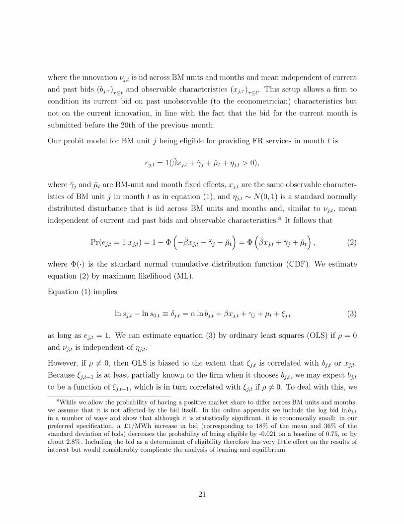
where the innovation νj,t is iid across BM units and months and mean independent of current

and past bids (bj,τ )τ≤t and observable characteristics (xj,τ )τ≤t. This setup allows a firm to

condition its current bid on past unobservable (to the econometrician) characteristics but

not on the current innovation, in line with the fact that the bid for the current month is

submitted before the 20th of the previous month.

Our probit model for BM unit j being eligible for providing FR services in month t is

ej,t = 1(βxj,t + γj + µt + ηj,t > 0),

where γj and µt are BM-unit and month fixed effects, xj,t are the same observable character-

istics of BM unit j in month t as in equation (1), and ηj,t ∼ N(0, 1) is a standard normally

distributed disturbance that is iid across BM units and months and, similar to νj,t, mean

independent of current and past bids and observable characteristics.8 It follows that

Pr(ej,t = 1|xj,t) = 1− Φ(−βxj,t − γj − µt

)= Φ

(βxj,t + γj + µt

), (2)

where Φ(·) is the standard normal cumulative distribution function (CDF). We estimate

equation (2) by maximum likelihood (ML).

Equation (1) implies

ln sj,t − ln s0,t ≡ δj,t = α ln bj,t + βxj,t + γj + µt + ξj,t (3)

as long as ej,t = 1. We can estimate equation (3) by ordinary least squares (OLS) if ρ = 0

and νj,t is independent of ηj,t.

However, if ρ 6= 0, then OLS is biased to the extent that ξj,t is correlated with bj,t or xj,t.

Because ξj,t−1 is at least partially known to the firm when it chooses bj,t, we may expect bj,t

to be a function of ξj,t−1, which is in turn correlated with ξj,t if ρ 6= 0. To deal with this, we

8While we allow the probability of having a positive market share to differ across BM units and months,we assume that it is not affected by the bid itself. In the online appendix we include the log bid ln bj,tin a number of ways and show that although it is statistically significant, it is economically small: in ourpreferred specification, a £1/MWh increase in bid (corresponding to 18% of the mean and 36% of thestandard deviation of bids) decreases the probability of being eligible by -0.021 on a baseline of 0.75, or byabout 2.8%. Including the bid as a determinant of eligibility therefore has very little effect on the results ofinterest but would considerably complicate the analysis of leaning and equilibrium.

21

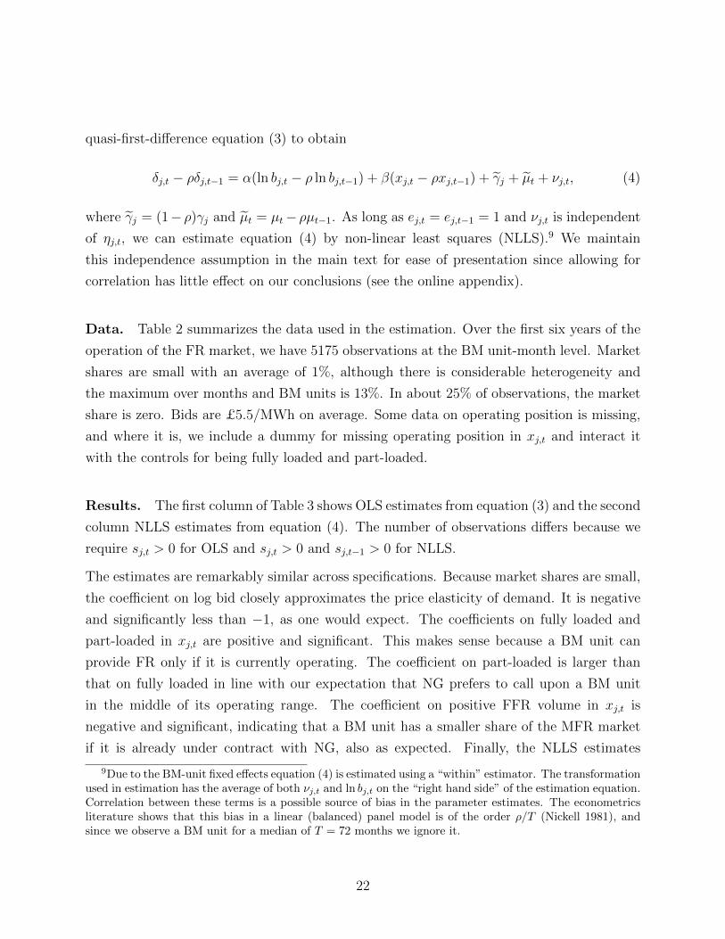
quasi-first-difference equation (3) to obtain

δj,t − ρδj,t−1 = α(ln bj,t − ρ ln bj,t−1) + β(xj,t − ρxj,t−1) + γj + µt + νj,t, (4)

where γj = (1− ρ)γj and µt = µt− ρµt−1. As long as ej,t = ej,t−1 = 1 and νj,t is independent

of ηj,t, we can estimate equation (4) by non-linear least squares (NLLS).9 We maintain

this independence assumption in the main text for ease of presentation since allowing for

correlation has little effect on our conclusions (see the online appendix).

Data. Table 2 summarizes the data used in the estimation. Over the first six years of the

operation of the FR market, we have 5175 observations at the BM unit-month level. Market

shares are small with an average of 1%, although there is considerable heterogeneity and

the maximum over months and BM units is 13%. In about 25% of observations, the market

share is zero. Bids are £5.5/MWh on average. Some data on operating position is missing,

and where it is, we include a dummy for missing operating position in xj,t and interact it

with the controls for being fully loaded and part-loaded.

Results. The first column of Table 3 shows OLS estimates from equation (3) and the second

column NLLS estimates from equation (4). The number of observations differs because we

require sj,t > 0 for OLS and sj,t > 0 and sj,t−1 > 0 for NLLS.

The estimates are remarkably similar across specifications. Because market shares are small,

the coefficient on log bid closely approximates the price elasticity of demand. It is negative

and significantly less than −1, as one would expect. The coefficients on fully loaded and

part-loaded in xj,t are positive and significant. This makes sense because a BM unit can

provide FR only if it is currently operating. The coefficient on part-loaded is larger than

that on fully loaded in line with our expectation that NG prefers to call upon a BM unit

in the middle of its operating range. The coefficient on positive FFR volume in xj,t is

negative and significant, indicating that a BM unit has a smaller share of the MFR market

if it is already under contract with NG, also as expected. Finally, the NLLS estimates

9Due to the BM-unit fixed effects equation (4) is estimated using a “within” estimator. The transformationused in estimation has the average of both νj,t and ln bj,t on the “right hand side” of the estimation equation.Correlation between these terms is a possible source of bias in the parameter estimates. The econometricsliterature shows that this bias in a linear (balanced) panel model is of the order ρ/T (Nickell 1981), andsince we observe a BM unit for a median of T = 72 months we ignore it.

22

Table 2: Summary Statistics (top 10 firms only)

Mean Std. Dev. Min MaxShare 0.011 0.016 0.000 0.131Eligibility 0.752 0.432 0.000 1.000Bid 5.453 2.759 1.515 21.003Fully loaded 0.133 0.236 0.000 0.997Part loaded 0.551 0.373 0.000 1.000Missing operating position 0.115 0.319 0.000 1.000Positive FFR volume 0.007 0.085 0.000 1.000Number of observations 5175

Summary statistics on the frequency response market. An observation is a bmunit-month, and the sample isrestricted to units owned by the top 10 biggest firms (ranked by revenue over the sample period). Eligibilityis an indicator for a bmunit receiving positive share. Fully loaded is the fraction of time the unit’s finalphysical notification is that it is fully loaded (i.e. operating at or close to capacity). Part loaded is thecorresponding fraction when it is operating below capacity. FFR volume is the quantity of FR providedthrough firm frequency response contracts (i.e. outside of this market).

from equation (4) in the second column of Table 3 provide evidence of persistence in the

unobservable characteristics ξj,t as the AR(1) coefficient ρ is positive and significant.

The third column of Table 3 shows ML estimates from equation (2). They are in line with

our logit model for market shares. In particular, the coefficients on fully loaded and part-

loaded are positive and significant, indicating that a BM unit is more likely to be eligible for

providing FR services if it is up and running.

To assess goodness of fit, we predict the market share of BM unit j in month t conditional on

sj,t > 0. To do so, we sample independently and uniformly from the empirical distribution

of residuals ξj,t for the OLS specification in equation (3) and from the empirical distribution

of residuals νj,t for the NLLS specification in equation (4).10 In both cases we repeatedly

10In the latter case, we proceed as follows: We first obtain the residuals νj,t along with the estimated

parameters α and β from equation (4). We then rewrite equation (3) as δj,t−α ln bj,t−βxj,t = γj +µt+ ξj,t,

substitute in α and β, and estimate by OLS. This yields the residuals ξj,t along with the estimated BM-unit

and month fixed effects γj and µt. We simulate ξj,t by substituting ξj,t−1 and a draw from the empiricaldistribution of residuals νj,t into the law of motion ξj,t = ρξj,t−1 + νj,t. If BM unit j has a zero share inmonth t− 1 so ξj,t−1 is missing, then we go back to the first month τ1 < t− 1 such that sj,τ1 > 0 and we goforward to the first month τ2 > t− 1 such that sj,τ2 > 0. We assume that νj,l = ν for all l = τ1, . . . , τ2 and

solve the equations ξj,t−1 = ρt−1−τ1ξj,τ1 + ν∑t−1−τ1−1l=0 ρl and ξj,τ2 = ρτ2−t+1ξj,t−1 + ν

∑τ2−tl=0 ρl for ν and

ξj,t−1. If missing for a stretch at the beginning so that τ1 is not defined, then we use the second equationalone with ν = 0; if missing for a stretch at the end so that τ2 is not defined, then we use the first equationalone with ν = 0.

23

Table 3: Demand System Estimates

Market Share EligibilityOLS NLLS ML

Log bid -1.648*** -1.614***(0.132) (0.119)

Fully loaded 1.666*** 1.949*** 2.501***(0.220) (0.182) (0.355)

Part loaded 2.111*** 2.234*** 2.168***(0.156) (0.139) (0.335)

Positive FFR volume -0.794*** -0.587** -0.500(0.200) (0.245) (0.461)

Unit and Month FE yes yes yesρ – 0.41 –s.e. ρ – 0.03 –Estimated R2 (of shares) 0.49 0.67 –N 3831 3509 5175

In the first two columns, the dependent variable is the log ratio of the share to the outside good share. Inthe last column it is an indicator for eligibility. The second market share specification allows for an AR(1)process in the error term, and we estimate the quasi-first-differenced equation by non-linear least squares(we provide an estimate of the autocorrelation coefficient ρ and the standard error of that estimate). TheR2 measure reported is for the fit of predicted versus actual shares (again omitting zero-share observations).Standard errors are clustered by bmunit. Significance levels are denoted by asterisks (* p < 0.1, ** p < 0.05,*** p < 0.01).

sample to integrate out over the empirical distribution of residuals. The logit model fits the

data reasonably well. Comparing realized and our predicted market shares from equation (3)

and equation (4), we get an estimated R2 of 0.49 and 0.67. This reinforces the importance

of persistence in the unobservable characteristics ξj,t and prompts us to take the NLLS

estimates from equation (4) in the second column of Table 3 as our leading estimates.

Figure 12 shows that the fit is good even for the largest power stations, whose market shares

change quite dramatically from one month to the next. This indicates that the good fit is

not solely a consequence of having BM-unit fixed effects.11

11We have done a number of robustness checks. The most notable is that the estimate for α decreasesfrom −1.614 in the middle column of Table 3 to −1.801 if we instrument for ln bj,t in equation (4). To doso, we first regress ln bj,t on δj,t−1, ln bj,t−1, xj,t, xj,t−1, and BM-unit and month fixed effects γj and µt and

predict ln bj,t. We then replace ln bj,t by ln bj,t in equation (4) and estimate by NLLS. While the estimatefor α decreases, the estimate for β remains virtually unchanged. We find the same if we additionally includebj,t−2 in the first-stage regression. These changes are not large enough to affect our conclusions.

24

.1.2

.3.4

.5S

hare

0 20 40 60 80Month

DRAXX

0.0

5.1

.15

.2.2

5S

hare

0 20 40 60 80Month

EGGPS0

.05

.1.1

5.2

Sha

re

0 20 40 60 80Month

RATS

0.0

5.1

.15

.2S

hare

0 20 40 60 80Month

BARK

Figure 12: Goodness of fit. Realized (blue, solid) and predicted (red, dashed) market shareby month for the four largest power stations Drax (top left panel), Eggborough (top rightpanel), Ratcliffe (bottom left panel), and Barking (bottom right panel).

4.2 Cost

Since the firms we are modeling have been providing FR for a long time, we assume that they

know their cost. However, we as researchers do not. With demand estimated, we therefore

turn to estimating cost since cost is an input to the learning models in Section 5.

The main source of cost is the additional wear and tear that a BM unit incurs while in FR

mode, which we expect to be relatively stable over time. Let cj denote the constant marginal

cost of BM unit j for providing FR. The realized profit of firm i in month t is

πi,t =∑j∈Ji

(bj,t − cj)Mtsj(bt, xt, ξt, et; θ0), (5)

25

where Mt is market size in month t and our notation emphasizes that the market share of

BM unit j in month t depends on the bids bt, characteristics xt and ξt, eligibilities et of

all BM units, as well as on the true parameters θ0 of the demand system. In contrast to

market share, market size Mt is independent of bids bt because the response requirement NG

is obligated to satisfy is exogenously determined by government regulation as a function of

the demand for electricity.

We estimate the marginal cost ci = (cj)j∈Ji for the BM units that are owned by firm i from

the bidding behavior of the firm in the late or stable-price phase of the FR market from

June 2009 to October 2011. We maintain that a firm’s bidding behavior stems from the firm

“doing its best” in the sense of choosing its bid to maximize its expected profit conditional

on the information available to it. More formally, the bids bi,t of firm i in month t ≥ 44

maximize the firms’ perception of expected profit conditional on the information it has at

its disposal at the time the bid is submitted:

maxbi,tEb−i,t,ξt,et,θt

[∑j∈Ji

(bj,t − cj)Mtsj(bt, xt, ξt, et; θt)

∣∣∣∣Ωi,t−1

], (6)

where in a slight abuse of notation we use Ωi,t−1 to denote both the firm’s perceptions and

its information per se. The notation in equation (6) is designed to stress the two main

sources of uncertainty that a firm faces, namely (i) strategic uncertainty about its rivals’

bids b−i,t and (ii) demand uncertainty generated by the realizations of ξt and et and the fact

that the parameters θt of the demand model may not be known (so to the firm the demand

parameters are a random variable). Using the information available to it, the firm forms

perceptions about b−i,t, ξt, et, and θt.12 These perceptions underlie the expectation operator

Eb−i,t,ξt,et,θt [·|Ωi,t−1] in equation (6). How perceptions are formed is the central question for

the learning models that we turn to in Section 5, but for now we remain agnostic.

Equation (6) does imply that the firm believes its current bids do not impact future profit,

and because of this rules out most models of experimentation. It is therefore not an ap-

propriate characterization of the bidding behavior in the early phase of the FR market. It

also rules out collusive equilibria, since in that case firms would act to maximize a different

objective function. We come back to the possibility of collusion below.

12We make the simplifying assumption that the firm has perfect foresight about market size Mt and thecharacteristics xt to avoid modeling their perceptions about these objects.

26

Equation (6) implies that the bids bi,t of firm i in month t ≥ 44 solve the first-order conditions

Eb−i,t,ξt,et,θt

[Mtsk(bt, xt, ξt, et; θt) +

∑j∈Ji

(bj,t − cj)Mt∂sj(bt, xt, ξt, et; θt)

∂bk,t

∣∣∣∣Ωi,t−1

]= 0, ∀k ∈ Ji.

(7)

Since we have not specified how the firm forms its perceptions, the system of first-order

conditions in equation (7) does not provide the restrictions needed for estimating marginal

cost (our ci). To derive an estimator for ci we use a relatively weak rationality assumption

that restricts perceptions in a way that we view as appropriate for the late phase.

By the time the FR market enters the late phase, a firm has had ample opportunity to

observe how its rivals bid as well as the resulting allocation of market shares. There are

changes in the physical environment during the late period, and these do cause changes in

bids, but we assume that the firm’s bids are by now free of bias. That is, we find our estimate

of ci by first substituting the realized market size Mt and market shares si,t = (sj,t)j∈Ji for

the BM units that are owned by firm i as well as our estimate α from Table 3 into equation

(7) and then setting the time-average of the first-order conditions for months t ≥ 44 to zero,

or1

29

T=72∑t=44

[Mtsk,t +

∑j∈Ji

(bj,t − cj)Mt (1(k = j)− sk,t)αsj,tbk,t

]= 0, ∀k ∈ Ji, (8)

where we have substituted out for the derivatives in equation (7) using the properties of

the logit and 1(·) is the indicator function. We estimate ci by solving this system of |Ji|equations for the |Ji| unknowns. This is straightforward because the equations are linear in

the unknowns.

Given the behavioral assumption in equation (6), a sufficient condition for our estimation

procedure to yield a consistent estimate of ci as the time horizon T → ∞ are that (i) our

estimate of θ is consistent for that parameter, (ii) the firm’s perceptions about b−i,t, ξt, et,

and θt lead to an unbiased estimate of the time-averaged first-order conditions in equation

(8) as T →∞, and (iii) values of ci different from the true marginal cost ci lead to values of

the time-averaged first-order conditions that are bounded away from zero as T →∞.13

The behavioral assumption in equation (6) is standard: the econometrician has to under-

stand the incentives faced by the firm in order to use the implications of the firm’s actions

13Formally, let yi,t ≡ (Mt, bi,t, si,t) and define hk(ci, α, yi,t) ≡ Mtsk,t +∑j∈Ji

(bj,t − cj)Mt (1(k = j)− sk,t) αsj,tbk,t, and h(ci, α, yi,t) ≡

[h1(ci, α, yi,t), . . . , h

Ji(ci, α, yi,t)]′

. Let

27

in estimation. The consistency condition (i) and the identification condition (iii) are also

standard (if the objective function cannot asymptotically distinguish the true marginal cost

from alternative values identification is hopeless). But notice that we have not specified

how a firm forms its perceptions. We do not have to assume that the market is in a “ratio-

nal expectations” equilibrium or that the environment necessarily reaches some sort of rest

point (neither the actual nor the perceived distribution of bids have to be stationary). We

do, however, require that the average of the firm’s perceptions of its first-order conditions

converges to the true average over time. Although we think of this as a weak rationality

condition, determining which learning models satisfy it is a problem that we leave to future

research. However, in the appendix we show that a sufficient condition for such convergence

is that the subjective probability distribution underlying the firm’s perceptions converges

weakly to the objective probability distribution (uniformly across information sets).

Results: estimates. The average of the marginal costs cj that we estimate for the J = 72

BM units owned by the ten largest firms is £1.40/MWh, with a standard deviation of

£0.66/MWh across BM units.14 The estimates are reasonably precise, with an average

standard error of £0.04/MWh. By comparison, pre CAP047 the “cost reflective” adminis-

tered price was around £1.7/MWh.15 Since we expect some markup to be built into the

administered price, the marginal costs we recover are in the right ballpark.

Table 4 shows the average marginal cost for the BM units belonging to the eight largest

power stations. They are quite reasonable and vary between £1.04/MWh and £1.6/MWh

across stations. The standard deviation of marginal cost within a station is very small, on

the same order as the standard error of the estimates. Most of the variation in marginal cost

is therefore across stations.

hTi,t(ci) = h(ci, αT , yi,t) and hei,t(ci) = Eb−i,t,ξt,et,θt [h(ci, α, yi,t)|Ωi,t−1]. We require that

‖T−1T∑

t=44

(hTi,t(ci)− hei,t(ci)

)‖ = op(1) and sup

‖ci−ci‖≥ε‖T−1

T∑t=44

hTi,t(ci)‖−1 = Op(1), ∀ε > 0,

where ‖ · ‖ is the Euclidean norm, op(1) indicates convergence in probability to zero, and Op(1) indicatesstochastically bounded. The proof of consistency follows from Theorem 3.1 in Pakes and Pollard (1989).

14Because one BM unit has zero share during the late phase, we impute its marginal cost with that of theother BM unit in the same power station.

15We have two sources: Figure 2 and a document prepared just prior to CAP047 by NG for Ofgem, thegovernment regulator (www.ofgem.gov.uk/ofgem-publications/62273/8407-21104ngc.pdf). It states inparagraph 5.3 that the holding payment is “of the order of £5/MWh” for the bundle of primary, secondary,and high response, implying an average of £1.67/MWh per type of FR.

28

Table 4: Cost estimates for the top 8 stations (by total revenue)

Station # Units Fuel Vintage Mean Std. Dev. (within station)

Barking 2 CCGT 1994 1.2 .01Connah’s Quay 4 CCGT 1996 1.04 .03Cottam 4 Coal 1969 1.35 .04Drax 6 Coal 1974 1.06 .04Eggborough 4 Coal 1968 1.53 .06Peterhead 1 CCGT 2000 1.54 0Ratcliffe 4 Coal 1968 1.33 .06Seabank 2 CCGT 1998 1.59 .01

Summary statistics on the unit-specific cost estimates derived from solving the firm first order conditionarising from the demand system, reported as the within-station average cost and standard deviation incosts.

Table 5 shows the result of regressing marginal cost on the characteristics of the BM units.

As expected, a (typically smaller) BM unit using dual fuel or oil has lower cost than a BM

unit using other fuel types. Moreover, although not statistically significant, the estimates

suggest that a BM unit of later vintage has lower cost.

Results: residuals. Using our estimates, we evaluate month-for-month the realized value

of the profit derivative Mtsk,t+∑

j∈Ji (bj,t − cj)Mt (1(k = j)− sk,t) αsj,tbk,t

in equation (8). For

simplicity, we call this value a “residual.” By construction, the residual is zero on average

across months for all BM units in the late phase of the FR market. Figure 13 shows the time

series of the average residual across BM units. It contrasts the early and middle phases in

the left panel with the late phase of the FR market in the right panel. The average residual

starts well above zero in the early phase before falling below zero in the middle phase. The

standard deviation falls throughout, consistent with our earlier discussion of convergence.

In the late phase, the average residual is above zero in some months and below zero in others

and the standard deviation does not exhibit a trend. Interestingly, even after the substantial

increase in FFR volume that occurs in July 2010 (see again Figure 4, we indicate July 2010

with a dashed line in the right panel of Figure 13) and changes in participation during this

phase (see Figure 5), the average residual continues to be zero and the standard deviations

are still an order of magnitude smaller than in the early phase of the FR market. Apparently

in the late phase firms adjust to changes in their environment quite quickly. This is quite

different than the behavior in the earlier phases.

29

Table 5: Projecting costs onto unit characteristics

Cost estimateUnit vintage -0.015

(0.017)Dual Fuel -0.819*

(0.466)Large Coal -0.463

(0.429)Medium Coal -0.683

(0.544)Oil -0.967**

(0.397)

R2 0.13N 71

The dependent variable is the cost estimate cj . The omitted fuel type is combined cycle gas turbines (CCGT).One observation is dropped because of missing vintage data. Significance levels are denoted by asterisks (*p < 0.1, ** p < 0.05, *** p < 0.01).

We also examine whether the residuals are autocorrelated. The first three columns of Table 6

display the coefficients from separate regressions of the residual on its lagged value for each

of the three phases of the FR market, including BM-unit fixed effects in all regressions. In

the last three columns we further restrict attention to observations in which the BM unit’s

bid changed between months.

We find significant autocorrelation in all regressions but the last. Assuming our specification

and cost estimates are correct, this indicates that some firms are making systematic mistakes.

This may reflect persistent differences between a firm’s perceptions of its expected profits

and reality. This makes particular sense in the early and middle phases of the FR market

where firms had little experience and behaved quite differently.

At the same time, it is striking how the R2 falls over the three phases of the FR market,

indicating that the lagged value explains progressively less of the variation in the residual.

In the third phase, we find significant autocorrelation using all observations (third column),

but that essentially disappears when we restrict attention to observations in which the BM

unit’s bid changed between months (last column). Our interpretation of this is that by the

end firms have reasonably accurate perceptions, and when they choose to update their bids

they do so in a way that accounts for the information contained in the lagged residual.

30

050

0010

000

2005m7 2006m7 2007m7 2008m7 2009m7monthyear

Average residual Standard deviation of residuals

−10

000

1000

2000

3000

2009m7 2010m1 2010m7 2011m1 2011m7monthyear

Average residual Standard deviation of residuals

Figure 13: Average and standard deviation of residuals during the early and middle phases(left panel) and late phase (right panel). In the right panel, the dotted line indicates July2010, when FFR volume nearly doubles.

Timing of bid changes and ex-post profitability. One of the striking empirical reg-

ularities of the data is that some firms take a far more active approach to bidding than

others. This is documented in Table 7, where we count the number of months in which a

firm updated the bid of any of its BM units. E.ON, Barking, and Centrica change their bids

in more than half of the months, but the remainder of the top 10 firms (notably including

Drax) make changes far less frequently. The frequency of bid changes is not significantly

correlated with firm size as measured by realized profit over the full sample period: the three

most active firms are ranked second, sixth and tenth in terms of firm size.

To get a sense of how costly this infrequent adjustment may be, we use our demand and

cost estimates to compute a firm’s the ex-post optimal bid b∗i,t given the realizations of b−i,t,

ξt, and et. The ex-post optimal bid can be computed without committing to a particular

model of how the firm forms perceptions, and therefore allows us to offer statistics that are

more “model-free” than those in the learning analysis below. We moreover define the ex-post

lost profit as the difference between profit at the ex-post optimal bid b∗i,t and profit at the

observed bid bi,t.

Somewhat surprisingly, the ex-post lost profit does not allow us to explain the timing of bid

changes. We would expect firms to be more likely to adjust their bids in months where the

ex-post lost profit is large, but we find no statistically significant support for this in any of

a number of probit regressions that explore different plausible specifications.

31

Table 6: Autocorrelation in residuals

Early Middle Late Early Middle LateAll Bid changes only

Lagged residual 0.542*** 0.343*** 0.445*** 0.389*** 0.126*** 0.029(0.087) (0.050) (0.063) (0.059) (0.042) (0.080)

R2 0.63 0.48 0.20 0.74 0.38 0.08N 1080 1931 2088 355 449 401

The dependent variable is the residual in the FOC at the estimated costs. Controls are the lagged residualand unit fixed effects. The regressions with bid changes only include only observations in which the unit’sbid was different from its bid in the previous period. Standard errors are clustered by unit. Significancelevels are denoted by asterisks (* p < 0.1, ** p < 0.05, *** p < 0.01).

However, the ex-post optimal bid helps to explain the direction in which firms adjust their

bids, conditional on adjusting. The “matched direction” column in Table 7 indicates the

percentage of times that such adjustments are in the direction of the ex-post optimal bid

(share-weighting across the BM units within a firm). It is well above 50% for many firms.

For the most active firms we match the direction less often, consistent with our account of

firms “exploring” during the early phase of the FR market.

To measure how much money the firms have “left on the table” we look at the ex-post lost

profit over the full sample period as a percentage of realized profit in the sixth column of

Table 7. The magnitudes are generally small, which is striking given that the ex-post optimal

bid is computed using data the firms did not know at the time they made their bids.

For example, RWE plc rarely updated its bids and slowly tracked the market upwards.

As a result, we estimate that they lost £768,000 or 3.06% over six years. While this is

enough money that we may expect RWE plc to pay more attention and update its bids more

frequently, it is perhaps not enough to justify hiring a full-time employee to study the FR

market and optimize bidding.

Contrast these small ex-post profit differences with the average absolute difference between

a firm’s (share-weighted) average bid and the ex-post optimal bid, shown in the last two

columns in absolute and relative terms. These magnitudes are much larger, with most firms

placing bids that are around 15% to 20% away from their ex-post optimal bids.

This suggests a possible reason why we have been unable to explain the timing of bid changes:

some firms are paying infrequent attention to the FR market and making sensible but not

32

Table 7: Profit Statistics

Months Matched Total Ex-Post Ex-Post Ex-PostRank Firm name Changed Direction Profit Lost Bid Bid

(%) Profit (%) Diff. Diff. (%)

1 Drax Power Ltd. 23 80 68.4 2.03 1.1 202 E.ON UK plc 52 67 44.4 2.01 .76 143 RWE plc 15 86 25.1 3.06 .93 234 Eggborough Power Ltd 18 58 18.2 1.43 .84 175 Keadby Generation Ltd 17 80 14.9 5.12 1.03 196 Barking Power Ltd 57 49 11.8 6.17 .65 157 Jade Power Generation Ltd 15 54 10 4.74 1.24 248 SSE Generation Ltd 17 62 9.4 .47 .42 89 Seabank Power Ltd 9 89 9.1 8.21 1.14 2010 Centrica plc 42 73 8.7 2.59 .92 18

Months changed indicates the total number of months in which a firm changed the bid of one or more of theirunits. Matched direction indicates the share-weighted percent of bid changes that are in the same directionas our estimated ex-post-optimal bid. Ex-post lost profit indicates the share-weighted percent increase inprofit by taking the estimated ex-post-optimal bid instead of the actual bid. Ex-post bid difference indicatesthe share-weighted average absolute difference between the ex-post-optimal and actual bids, in absolute andrelative terms.

necessarily optimal adjustments when they do. This combination of rational inattention

(Sims 2003) and “satisficing” behavior (Simon 1955) may have been optimal along the ob-

served path of play given the firms’ various human resource and institutional constraints.

Yet, as Akerlof and Yellen (1985) have noted, even small departures from perfect rationality

may lead to aggregate behavior that is quite different from equilibrium and thus hard to

predict with equilibrium models. To investigate bidding incentives during the disequilibrium

phase of the observed play, we need the learning models that we outline in Section 5 below.

Collusion? Before doing so, we briefly examine the possibility of collusion between the

firms in our data. We try two different approaches. The first is to look for coordination in

the timing and direction of bid changes across BM units, as this could be a sign of collusion

being established or breaking down. To capture timing, we define a dummy for BM unit

j changing its bid between months t − 1 and t and, to capture direction, another dummy

for the BM unit increasing its bid. We compute all pairwise correlations between BM units

in the dummy for a BM unit changing its bid and in the dummy for a BM unit increasing

33

01

23

45

6D

ensi

ty

−1 −.75 −.5 −.25 0 .25 .5 .75 1R

01

23

45

6D

ensi

ty

−1 −.75 −.5 −.25 0 .25 .5 .75 1R

01

23

45

6D

ensi

ty

−1 −.75 −.5 −.25 0 .25 .5 .75 1R

01

23

45

6D

ensi

ty

−1 −.75 −.5 −.25 0 .25 .5 .75 1R

Figure 14: Top left is within-firm correlation in bid changes; top right is across-firm correla-tion in bid changes; bottom left is within-firm correlation in direction of change (conditionalon both changing); bottom right is across-firm correlation in directions.

its bid (conditional on both BM units in the pair changing their bids). In Figure 14 we

plot the distribution of correlation coefficients separately for BM units owned by the same

firm (“within firm”, left panels) and for BM units owned by different firms (“across firms”,

right panels). Note that we expect some across-firm correlation in both the timing and the

direction of bid changes due to common shocks to demand.

The within-firm correlations for the timing and direction of bid changes in the left panels

are positive and substantial. This reinforces our contention that decisions are centralized

at the level of the firm rather than made at the level of the BM unit. The right panels

show correlations pretty much evenly distributed around zero, consistent with independent

decision making across firms.

Our second approach is more direct: we assume particular collusive arrangements and infer

34

costs given the assumed conduct. Specifically, we re-solve equation (8) for the cost vector

that is consistent with observed play during the late phase of the FR market under the

assumption that the top 10 firms colluded and maximized the combined profits of all their

BM units. This yields an estimated average cost of £-9.8/MWh for the BM units, which is

negative and clearly implausible. The estimates are negative because demand is relatively

inelastic, and so rationalizing the bids in the face of increased market power requires firms

to have low costs. When we repeat the exercise assuming that only the top 3 firms collude,

the implied average costs are £-0.25/MWh, still negative. This suggests that there is little

or ineffective collusion during the late phase of the FR market. While we cannot rule

out collusion in the earlier phases — and indeed we believe Drax attempted to establish a

tacit collusive arrangement in the middle phase — the lack of significant bid correlation is

suggestive evidence against this.

Repositioning in the BM. One might worry that equation (5) does not reflect the full

set of incentives a firm faces, as it does not account for the profit that accrues to a BM unit

as it is repositioned in the BM in preparation for providing FR. In the online appendix, we

incorporate these incentives. Using additional data on the BM, we first model and estimate

demand for repositioning. Extending equation (8), we then simultaneously estimate the

marginal cost of providing FR and a markup on repositioning. The estimated markup is

very small and not statistically different from zero, and the marginal cost of providing FR

does not change materially from that reported earlier in this section.

The markup partly reflects the amount of attention paid to the profit from repositioning

when deciding on the FR bid. Our estimate may thus be explained by the fact that FR bids

and bids in the BM are made by different people within the firm, and those deciding on FR

bids may not pay attention to the BM. This is consistent with our conversations with Ian

Foy, who told us that people in the industry do not think of repositioning incentives when

deciding on FR bids.

5 Learning and equilibrium

In this section we consider how well different learning models fit the data. We noted in

Section 3 that realistically accounting for the bidding behavior in the early phase of the FR

35

market requires an explanation for the heterogeneity in the way firms learn and a model that

allows for experimentation. These are topics we do not tackle here. Instead, we consider

models of the bidding behavior in the middle and late phase of the FR market. The middle

phase is characterized by a convergence of bids in a relatively stable physical environment

whereas there are several environmental changes in the late phase.

Our learning models capture the two main sources of uncertainty that a firm faces, namely:

(1) strategic uncertainty about its rivals’ bids b−i,t, and (2) demand uncertainty generated

by the realizations of ξt and et and by the fact that the parameters θ of the logit model

may not be known. As noted in Section 1, the literature traditionally uses different types

of models for how a firm forms perceptions about rivals’ bids and for how the firm forms

perceptions about demand, and so do we. Our learning models combine fictitious play as a

model for learning about rival’s bids, and adaptive learning about demand.

Recall that prior to CAP047 providing FR was mandatory, so at the start of our study firms

already had quite a bit of experience with demand and cost. We therefore assume throughout

that firms know the marginal cost c of all BM units, the AR(1) process generating ξt, the

objective probability distribution of et, and the BM-unit fixed effects γ = (γj)j=1,...,J . The

latter capture the time-invariant preferences of NG for the different BM units. However,

there is reason to think firms had to learn about other aspects of demand. In particular,

since prior to CAP047 the holding payment was at an administered price which had been

fairly constant over time, firms may not have been able to assess the sensitivity of NG

to the bids they submit, a sensitivity captured by the parameter α in our model. They

may also have been uncertain about the parameter β to the extent that the time-varying

characteristics xj,t mattered differently for NG post CAP047. Finally, firms may have been

uncertain about the month fixed effect µt that subsumes any time-varying characteristics of

the outside good.

As a baseline we also compute a complete information Nash equilibrium. The literature

often refers to this rational-expectations model, so how it compares to our learning models

is of some interest.

5.1 Complete information Nash equilibrium

The assumptions underlying a complete information Nash Equilibrium are more restrictive

than those we needed for estimation in the cost estimation section: the bids b∗t of all BM

36

units solve the system of J equations

Eξt,et

[Mtsk(b

∗t , xt, ξt, et; θ0) +

∑j∈Ji

(b∗j,t − cj

)Mt

∂sj(b∗t , xt, ξt, et; θ0)

∂bk,t

∣∣∣∣Mt, xt, ξt−1, θ0, c

]= 0, ∀k = 1, . . . , J.

(9)

The notation Eξt,et [·|·] in equation (9), in contrast to Eb−i,t,ξt,et,θt [·|·] in equation (6), is

meant to indicate that the expectation is computed with respect to the objective probability

distribution of ξt and et conditional on the information available to firm i in month t − 1

when it submits its bids bi,t for month t. We assume that the firm has perfect foresight

about market size Mt, the observable characteristics xt, and that the marginal cost c of all

BM units are common knowledge. In addition, we condition the expectation operator on the

unobservable characteristics ξt−1 with the implicit understanding that ξj,t follows the AR(1)

process ξj,t = ρξj,t−1 + νj,t with ρ known. Finally, we abstract from uncertainty about the

parameters of the demand system for now and condition the expectation operator on θ0.

Later on we extend the complete information Nash equilibrium to accommodate adaptive

adaptive learning about demand.

Note that the expectation operator in equation (9) does not condition on b−i,t. While the

best response of firm i depends on its perceptions of its rivals’ bids, in a complete information

Nash equilibrium these perceptions are consistent with actual play. A complete information

Nash equilibrium is thus obtained by solving the above J equations in the J unknowns b∗t .

To make equation (9) practical we replace ξt−1, θ0, and c by our estimates of those objects and

evaluate the expectation operator using Monte Carlo integration. To this end we generate a

random sample(ξ

(s)t , e

(s)t

)s=1,...,S

with S = 50, 000 and replace the expectation operator by

the corresponding sample average. To obtain ξ(s)j,t , we sample independently and uniformly

from the empirical distribution of residuals νj,t from the NLLS specification in equation (4)

(for further details see again footnote 10). To obtain e(s)j,t , we sample independently from a

Bernoulli distribution with success probability Pr(ej,t = 1|xj,t) as specified in equation (2).

5.2 Learning models

We now explain in detail how in our learning models a firm forms perceptions about rivals’

bids and perceptions about demand.

37

Perceptions about rivals’ bids: fictitious play. Belief-based learning starts with the

premise that players keep track of the history of play and form beliefs about what their rivals

will do in the future based on their past play. We consider fictitious play as a leading example

of belief-based learning.16 In particular, we assume that in month t− 1 when firm i chooses

its bids bi,t it believes that its rivals’ bids b−i,t are sampled from the empirical distribution

of their past play. To account for correlation in the bids of firm i’s rivals, we sample an

entire vector of rivals’ bids. Since firm i may believe that its rivals’ bids b−i,t are more

similar to more recent observations, we allow for geometrically declining sampling weights.

In particular, we assign sampling weight δt−τ−1 to rivals’ bids b−i,τ in month τ ≤ t−1, where

δ ∈ [0, 1] is a decay parameter, and then normalize so the sampling weights sum to one. For

month τ = t−1, t−2, t−3, . . . the sampling weight is therefore proportional to 1, δ, δ2, . . ..17

We let F (δ) denote our model of fictitious play with decay parameter δ. Note that δ = 1

indicates no decay and δ = 0 full decay. Adaptive best response thus arises as a special case

of fictitious play for δ = 0. Under F (0) firm i believes that its rivals’ bids b−i,t in month t

are equal to its rivals’ bids b−i,t−1 in month t− 1 with certainty. In the other extreme, under

F (1) all past observations are weighted equally.

Perceptions about demand: adaptive learning. To account for uncertainty about de-

mand in addition to uncertainty about rivals’ bids, we allow a firm to adaptively learn about

the parameters θ of the logit model. Developed in the macroeconomics literature, adaptive

learning stipulates that agents learn about parameters in the same way as econometricians:

by using the available data to estimate them. As more data becomes available over time,

agents update their estimates.18

We focus on a simple form of adaptive learning that assumes that firms use the regression

procedure described in Section 4.1 and the data available to them to estimate the parameters

they are uncertain about (in month t−1 when preparing their bids bt for month t firms only

have data for month τ ≤ t − 2 at their disposal because NG does not publish quantities

for a month until the very end of the month). We refer to the estimates obtained in this

manner as the “sequential” estimates for month t and distinguish them from the “full-sample”

estimates obtained in Section 4.1. We assume throughout that firms ignore any uncertainty

16For a discussion of fictitious play and its possible variants see Fudenberg and Levine (1998).17In nine instances the bid bj,t of BM unit j in month t is missing. To facilitate sampling, we impute it

by going back in time to the first month τ < t such that bj,τ is not missing.18For a detailed treatment of adaptive learning see Evans and Honkapohja (2001).

38

in the sequential estimates so that their perceptions are a point mass on those estimates.

We noted above that there is reason to think that firms may have been uncertain about

the price sensitivity parameter α, about the coefficient β on the time-varying characteristics

xj,t, and about the month fixed effect µt. Accordingly, we distinguish four combinations of

parameters that firms may have been uncertain about, namely α, α and β, α and µt, and

α, β, and µt. Our notation for and implementation of adaptive learning for these four cases

plus the baseline case that abstracts from demand uncertainty is as follows:

1. A(α): Using data for month τ ≤ t − 2 and fixing β, ρ, γ, and (µτ )τ≤t−2 at the full-

sample estimates in Table 3, estimate equation (4) by OLS to obtain the sequential

estimate α(t) for month t.

2. A(α, β): Using data for month τ ≤ t − 2 and fixing ρ, γ, and (µτ )τ≤t−2 at the full-

sample estimates, estimate equation (4) by OLS to get the sequential estimates α(t)

and β(t) for month t.

3. A(α, µt): Using data for month τ ≤ t − 2 and fixing β, ρ, and γ at the full-sample

estimates, estimate equation (4) by OLS to obtain the sequential estimates α(t) and(µ(t)

τ

)τ≤t−2

for month t. Using data for month τ ≤ t − 2 and fixing β and γ at the

full-sample estimates and α at the sequential estimate for month t, estimate equation

(3) by OLS to obtain the sequential estimates(µ

(t)τ

)τ≤t−2

(for more details see footnote

10). Extrapolate µ(t)t = µ

(t)t−2 to obtain the sequential estimate µ

(t)t for month t.

4. A(α, β, µt): Using data for month τ ≤ t − 2 and fixing ρ and γ at the full-sample

estimates, estimate equation (4) by OLS to obtain the sequential estimates α(t), β(t),

and

(µ(t)

τ

)τ≤t−2

for month t. Using data for month τ ≤ t− 2 and fixing γ at the full-

sample estimate and α and β at the sequential estimates for month t, estimate equation

(3) by OLS to obtain the sequential estimates(µ

(t)τ

)τ≤t−2

. Extrapolate µ(t)t = µ

(t)t−2 to

obtain the sequential estimate µ(t)t for month t.

5. A(∅): Fix all parameters θ at the full-sample estimates in Table 3.

Predictions. We combine fictitious play with adaptive learning to make predictions. We

measure fit by comparing our predictions to the observed bids. We make two kinds of

39

predictions. The first is one-period predictions: for each month t during the second and

third phases, we take the data available to the firms at the time they bid (which includes

bids (br)r≤t−1 and market shares (sr)r≤t−2) and predict their bids. This corresponds to the

thought experiment of predicting the next move of a player in a game and is analogous to

the one-step-ahead predictions used to assess predictive accuracy in the experimental and

computational literatures (Erev and Roth 1998, Fershtman and Pakes 2012).

However, industrial organization analysts are often asked to predict how prices evolve for

many periods following a policy change or a change in market institutions. So we also

consider multi-period predictions in which we sequentially predict bids and market shares

and then overwrite the observed data with our predictions as we go. To see how these differ,

consider the following example: if the strategic model specifies that firms best respond to last

period’s bids, and we predict in period t that BM unit 1 bids 7 but it actually bids 11, then in

the one-period prediction exercise we predict that in period t+1 the other firms best respond

to the actual bid of 11, but in the multi-period prediction exercise they best respond to the

simulated bid of 7. This allows the possibility that our multi-period predictions increasingly

diverge from the observed data. Indeed, if the model is correct, then the variance of the

prediction error should grow with the distance between the base period and the period for

which we are predicting.

A fictitious play model F (δ) with δ ∈ [0, 1] and an adaptive learning model A(y) with

y ∈ α, (α, β), (α, β, µt), ∅ together with available data Dt determine a predicted bid b(δ,y)i,t

for firm i in month t. That bid b(δ,y)i,t solves the system of Ji equations

Eb−i,t,ξt,et,θt

[Mtsk(b

(δ,y)i,t , b−i,t, xt, ξt, et, θt)

+∑j∈Ji

(b

(δ,y)j,t − cj

)Mt

∂sj(b(δ,y)i,t , b−i,t, xt, ξt, et, θt)

∂bk,t

∣∣∣∣F (δ), A(y), Dt

]= 0, ∀k ∈ Ji. (10)

The notation Eb−i,t,ξt,et,θt [·|·] indicates that the expectation operator is with respect to the

subjective probability distributions of b−i,t and θt induced by F (δ) and A(y). To make

equation (10) practical we replace ξt−1 and c in Dt by our estimates. In the single-period

prediction exercises, we estimate θt for the adaptive learning model A(y) as detailed above

using the observed data for month τ ≤ t − 2. We evaluate the remaining random variables

in the expectation operator by drawing samples(b

(s)−i,t, ξ

(s)t , e

(s)t

)s=1,...,S

with S = 50, 000,

40

Table 9: Different Learning Models for Middle phase: Single-period predictions.

Average Diff: Predicted and Actual Bid Mean Square Error

A(∅) A(α) A(α, µ) A(α, β) A(α, β, µ) A(∅) A(α) A(α, µ) A(α, β) A(α, β, µ)F(0) -0.21 -0.11 1.42 0.61 1.02 1.23 1.21 4.67 2.20 3.22F(0.5) -0.20 -0.10 1.44 0.62 1.03 1.23 1.22 4.72 2.23 3.26F(1) -0.47 -0.38 1.10 0.31 0.70 1.55 1.43 3.01 1.53 2.09Eq. -0.42 -0.29 1.90 0.67 1.29 1.36 1.26 6.70 2.29 4.13

∗ F (x) denotes fictitious play with δ = x. A(x) denotes adaptive learning where all parametersexcept x are known and x is sequentially estimated. All statistics are share-weighted.

proceeding as in Section 5.1 for sampling ξ(s)j,t and e

(s)j,t . We sample b−i,t according to F (δ) on

the data bss≤t−1.

The multi-period prediction exercises are identical except for the data Dt: for any model

(F (δ), A(y)) we replace the observed bids and market shares during the second and third

phases with our predictions b(δ,y)t , thus changing what firms observe.19 This has two effects.

First, when sampling b−i,t according to F (δ), we now sample our predicted bids. Second,

when estimating θt, the dataset used for estimation now contains our predicted bids and

market shares. These effects generate differences between the single- and multi-period pre-

dictions. For reasons that will become clear below, for the multi-period prediction exercises

we only consider the adaptive learning models A(∅) and A(α).

5.3 Results

We measure the predictive accuracy of our various fictitious play and adaptive learning

models in two ways: using (i) the share weighted average difference between the predicted

and actual bids, where we average over BM units and months and (ii) the share weighted

mean square error of prediction. The share weighted average error may be a useful measure

if the goal is to predict the overall cost of the FR market to NG. The mean square error is

a traditional way of assessing goodness of fit. We begin with discussing how well different

learning models fit the data from the middle phase of the FR market and then move on to

the late phase.

19To predict market shares we use the estimated parameter vector θ regardless of the adaptive learningmodel A(y), as it is our best guess for that parameter.

41

Table 10: Different Learning Models for Middle phase: Multi-period predictions.

Average Diff: Predicted and Actual Bid Mean Square Error

A(∅) A(α) A(∅) A(α)F(0) -0.41 -0.21 1.31 1.22F(0.5) -0.39 -0.20 1.26 1.19F(1) -0.53 -0.38 1.46 1.33Eq. -0.42 -0.29 1.36 1.26

∗ F (x) denotes fictitious play with δ = x. A(x) denotes adaptive learning where all parametersexcept x are known and x is sequentially estimated. All statistics are share-weighted.

Middle or falling-price phase (March 2007 – May 2009). The two panels of Tables

9 and 10 summarize the share weighted average and mean square error for the middle phase

of the FR market in single-period and multi-period predictions respectively. Each panel

provides a two-way classification: The columns pertain to the baseline case A(∅) that ab-

stracts from demand uncertainty and the adaptive learning models A(α), A(α, β), A(α, µt),

and A(α, β, µt) (last three only in the single-period case). The rows pertain to the fictitious

play models F (0) (full decay or adaptive best response), F (0.5) (some decay), and F (1) (no

decay) and the complete information Nash equilibrium.

Starting with the single-period predictions, the 2 × 2 sub-matrix in the top left corner of

each panel of Table 9 has the smallest (in absolute value) entries. This pattern is starkest

in the average error in the left panel but also clearly present in the mean square error in the

right panel. Hence, under both accuracy measures, the preferred model for perceptions about

rivals’ bids is either F (0) or F (0.5). The preferred model for perceptions about demand is

either the baseline case A(∅) that abstracts from demand uncertainty or the adaptive learning

model A(α) that accounts for firms being uncertain about the price sensitivity parameter α,

with the average error indicating a slight preference for A(α) over A(∅). Extending adaptive

learning to additional parameters noticeably worsens goodness of fit under both accuracy

measures.

We have attempted to more finely determine the decay parameter δ in the fictitious play

model by conducting a grid search over δ = 0, 0.1, . . . , 1. While we obtain the smallest mean

square error at δ = 0.3, there is very little difference in mean square error as δ ranges from

0 to 0.6. Hence, all we can say is that the data from the middle phase of the FR market

appears to favor a fictitious play model in which firms rely disproportionately on more recent

observations to form beliefs about rivals’ bids.

42

A striking feature of Table 9 is that under both accuracy measures the fictitious play mod-

els F (0) and F (0.5) fit the data better than the complete information Nash equilibrium

irrespective of the particular adaptive learning model.

The complete information Nash equilibrium limits the range of the predicted price of FR.

This is perhaps unsurprising because ultimately only changes in the demand and cost primi-

tives can effect changes in the Nash equilibrium. In contrast, adaptive learning adds another

source of fluctuations in the predicted price of FR as perceptions about demand change with

more data becoming available to firms over time.

Turning to the multi-period predictions in Table 10, we see a qualitatively similar pattern.

The fictitious play models F (0) and F (0.5) continue to fit better than equilibrium, though

the differences in fit are in most cases smaller. Once again, F (0) and F (0.5) are hard to

distinguish.

One can more clearly compare single and multi-period predictions in Figure 15, where we

compare the time series of the predicted price under the model (F (0), A(α)) (the plot for

(F (0.5), A(α)) is similar) to the actual price and the complete information Nash equilibrium.

The single-period predictions matches the path better, which makes sense since they use

realized rather than predicted bids in making predictions. However, it is remarkable that

the multi-period predictions fit so well given that errors in predicting behavior have the

potential to accumulate as they form the basis for subsequent predictions. Instead, the

multi-period predictions roughly match the slow decline in prices that we see in the data.

This is not the case absent adaptive learning: according to the multi-period predictions from

the model (F (0), A(∅)), bids reach equilibrium levels within a few periods. However, if the

firm’s demand perceptions continue to evolve adaptively under the adaptive learning model

A(α), then it takes some time for the bids to reflect the actual value of α and this provides

a closer match to the data.

Late or stable-price phase (June 2009 - October 2011). Tables 11 and 12 are the

analogs for the late phase to Tables 9 and 10. The first thing to note from Table 11 and

Table 12 is that the mean square errors for both the single and the multi-period predictions

are much smaller than those for the middle phase. The mean square errors for either A(∅)or A(α) and either F (0) or F (.5) are about a third of the middle phase values, and they are

even a smaller fraction for the equilibrium predictions and other adaptive learning models.

Recall that, in contrast to the other phases, the late phase witnessed a number of changes in

43

Month15 20 25 30 35 40 45

Pric

e pe

r U

nit

4

4.5

5

5.5

6

6.5

7

7.5

Share-Weighted Multi-Period Estimated Bids [Best Response, Alpha Unknown]Share-Weighted Multi-Period Estimated Bids [Best Response, All Known]Share-Weighted Single-Period Estimated Bids [Best Response, Alpha Unknown]Share-Weighted Single-Period Estimated Bids [Equilibrium, All Known]Share-Weighted Actual Bids [Actual Price]

Figure 15: Predicted and actual FR price by month. Share-weighted average computedfrom bids predicted by fictitious play F (0) with adaptive learning A(α) in both single andmulti-period simulations, complete information Nash equilibrium without demand uncer-tainty A(∅), and actual bids. Middle phase.

the physical environment, so the improvement in fit may be surprising. On the other hand,

by the late phase firms had a lot of information on the likely responses of their competitors,

and this may have enabled quick adjustments to the environmental perturbations.

For the late phase it is more difficult to determine a preferred model for perceptions about

rivals’ bids from Table 11 and 12. While the data appear to favor the fictitious play models

F (0) and F (0.5) over F (1), both F (0) and F (0.5) are essentially indistinguishable from

the complete information Nash equilibrium. When we attempted to more finely determine

the decay parameter δ in the fictitious play model, there was a slight preference for δ = 0

(adaptive best response) in the single-period predictions but the difference from increasing δ

only becomes noticeable for δ > 0.6. In the late phase perceptions about competitors seem

to have “settled down,” and equilibrium predictions fit quite well.

It is similarly difficult to determine a preferred model for perceptions about demand. Looking

at the single-period models in Table 11, under both accuracy measures, the baseline case A(∅)

44

Table 11: Different Learning Models for Late phase: Single Period Predictions∗.

Average Diff: Predicted and Actual Bid Mean Square Error

A(∅) A(α) A(α, µ) A(α, β) A(α, β, µ) A(∅) A(α) A(α, µ) A(α, β) A(α, β, µ)F(0) 0.21 0.21 0.23 0.25 0.15 0.40 0.40 0.44 0.48 0.43F(0.5) 0.22 0.22 0.24 0.26 0.15 0.41 0.41 0.44 0.50 0.44F(1) 0.32 0.33 0.35 0.37 0.26 0.52 0.53 0.58 0.64 0.55Eq. 0.25 0.25 0.29 0.30 0.16 0.42 0.42 0.49 0.52 0.42

∗ F (x) denotes fictitious play with δ = x. A(x) denotes adaptive learning where all parametersexcept x are known and x is sequentially estimated. All statistics are share-weighted.

Table 12: Different Learning Models for Late phase: Multi-period predictions∗.

Average Diff: Predicted and Actual Bid Mean Square Error

A(∅) A(α) A(∅) A(α)F(0) 0.23 0.31 0.40 0.46F(0.5) 0.23 0.30 0.40 0.45F(1) 0.23 0.31 0.42 0.49Eq. 0.25 0.25 0.42 0.42

∗ F (x) denotes fictitious play with δ = x. A(x) denotes adaptive learning where all parametersexcept x are known and x is sequentially estimated. All statistics are share-weighted.

that abstracts from demand uncertainty and the adaptive learning models A(α), A(α, β),

and A(α, µt) are very similar to one another. The surprise is that the adaptive learning

model A(α, β, µt) has the smallest average error in predicting the (share weighted) average

bid (irrespective of the particular fictitious play model). Recall that our logit model for

market shares is an approximation of the true underlying demand. During the late phase

small changes in the physical environment occur periodically. Although the true underlying

demand is stationary, our best approximation to it may not be in light of these changes. A

possible explanation for the fact that A(α, β, µt) has the smallest average error may therefore

be that A(α, β, µt) has more free parameters than the other adaptive learning models and is

thus able to provide a better approximation to the demand systems when there are changes

in the institutional environment.

Figure 16 is the analog for the late phase to Figure 15. It shows clearly that in this phase both

the single and multi-period predictions from the model (F (0), A(∅)) make similar predictions

to the complete information Nash equilibrium. Thus the multi-period predictions converge

to the complete information Nash equilibrium, and at a rate that matches what we observe

45

Month40 45 50 55 60 65 70 75

Pric

e pe

r U

nit

4

4.5

5

5.5

6

6.5

7

7.5

Share-Weighted Multi-Period Estimated Bids [Best Response, Alpha Unknown]Share-Weighted Multi-Period Estimated Bids [Best Response, All Known]Share-Weighted Single-Period Estimated Bids [Best Response, Alpha Unknown]Share-Weighted Multi-Period Estimated Bids [Equilibrium, All Known]Share-Weighted Actual Bids [Actual Price]

Figure 16: Predicted and actual FR price by month. Share-weighted average computedfrom bids predicted by fictitious play F (0) with adaptive learning A(α) in both single andmulti-period simulations, complete information Nash equilibrium without demand uncer-tainty A(∅), and actual bids. Middle phase.

in the data. Convergence is not generally guaranteed under fictitious play (Fudenberg and

Levine 1998), so this is an indication that our pricing game is “well-behaved.”

Summary. Different models may be appropriate for different periods in an industry’s

evolution. In periods shortly after a major change in the environment, it may be better to

rely on models that allow for learning than to rely on equilibrium for one’s understanding of

— and one’s predictions for — behavior. This is true of the middle phase of the FR market

for single-period predictions and to an even larger extent for multi-period predictions, as

fictitious play models provided a substantially better fit than standard equilibrium notions.

We also observe in our data that incorporating uncertainty about demand through adaptive

learning models improves predictions for the middle phase. Moreover, all of the learning

models make multi-period predictions that converge and are virtually indistinguishable from

equilibrium predictions for the third phase. On the other hand, in the third phase of the FR

46

market, after firms had more experience interacting with their competitors, the equilibrium

model performs about as well as the best fitting learning models, and this occurs despite

smaller environmental changes that were largely absent in the earlier phases.

6 Conclusion

We have analyzed the evolution of the FR market in the UK following its deregulation. We

find that the market converged to a rest point after about three and a half years or 42 periods

of interaction. This rest point is consistent with a complete information Nash equilibrium

in that cost estimates derived using this assumption are plausible. There is substantial

heterogeneity in how the main market participants approach this rest point. Early on some

firms experiment, while others are more cautious and make infrequent adjustments. During

the middle phase, firm behavior is more predictable: bid predictions from fictitious play

models in which firms best respond to recent rival behavior are able to explain a substantial

share of the bid variance. The fit is further improved by allowing for adaptive learning

about the price parameter. These models match the observed bids better than assuming

equilibrium play; equilibrium predictions approach the rest point more rapidly than actual

play does. Moreover, the combination of best fitting learning models seems to converge to

a Nash equilibrium which is very close to the play we observe in the final phase. In the

final phase, that is after firms had quite a bit of data on the play of their competitors, the

equilibrium predictions fit about as well as the best fitting learning models and seem to

adjust rapidly to further changes in the environment.

Our empirical “case study” supports the idea that in stable environments play will generally

converge to a Nash equilibrium. This is consistent with the theory of learning in games, and

the corresponding idea that equilibrium play is a good prediction for the long-run outcome

of a game with strategic players. But for predicting short-run play following a change in

the environment, there are a variety of potential approaches. Here we find that models of

fictitious play and adaptive learning outperform full-information equilibrium predictions, at

least in the second phase of the data, and lead to behavior which is almost indistinguishable

from the actual play in the final period we study. This lends empirical support to these

learning models, which to the best of our knowledge have thus far only been tested in the

lab. We would thus argue that some thought is warranted before imposing equilibrium play

in counterfactual analysis, especially when a short-term prediction is needed.

47

Finally, we note that firms were heterogeneous in their activity levels in a way that is hard

to explain through profit motives alone. Firms also did not fully optimize their bids, but

this cost them little in forgone profits. This suggests that organizational analysis — or at

least some robustness to organizational inertia and imperfect optimization — would also be

helpful in predicting market evolution.

References

Ackerberg, Daniel A., “Advertising, Learning, and Consumer Choice in Experience Good

Markets: An Empirical Examination,” International Economic Review, 2003, 44 (3),

1007—1040.

Akerlof, George and Janet Yellen, “Can Small Deviations from Rationality Make Sig-

nificant Differences to Economic Equilibria?,” The American Economic Review, 1985,

75 (4), 708–720.

Anufriev, Mikhail and Cars Hommes, “Evolutionary Selection of Individual Expec-

tations and Aggregate Outcomes in Asset Pricing Experiments,” American Economic

Journal: Microeconomics, 2012, 4 (4), 35–64.

Benkard, C. Lanier, “Learning and Forgetting: The Dynamics of Aircraft Production,”

American Economic Review, 2000, 90 (4), 1034–1054.

Bergeman, Dirk and Juuso Valimaki, “Learning and Strategic Pricing,” Econometrica,

1996, 64 (5), 1125–1149.

and , “Dynamic Price Competition,” Journal of Economic Theory, 2006, 127,

232–263.

Bernhardt, Dan and Bart Taub, “Learning About Common and Private Values in

Oligopoly,” Rand Journal of Economics, 2015, 46 (1), 66–85.

Bolton, Patrick and Christopher Harris, “Strategic Experimentation,” Econometrica,

1999, 67 (2), 349–374.

Borenstein, Severin, James B. Bushnell, and Frank A. Wolak, “Measuring Mar-

ket Inefficiencies in California’s Restructured Wholesale Electricity Market,” American

Economic Review, 2002, 92 (5), 1376–1405.

48

Borgers, Tilman and R. Sarin, “Learning Through Reinforcement and Replicator Dy-

namics,” Journal of Economic Theory, 1997, 77 (1–14).

Brown, G.W., “Iterative Solutions of Games by Fictitious Play,” in T.C. Koopmans, ed.,

Activity Analysis of Production and Allocation, Wiley, 1951.

Camerer, Colin and Teck-Hua Ho, “Experienced-Weighted Attraction Learning in Nor-

mal Form Games,” Econometrica, jul 1999, 67 (4), 827–874.

, , and Juin-Kuan Chong, “Sophisticated Experience-Weighted Attraction

Learning and Strategic Teaching in Repeated Games,” Journal of Economic Theory,

2002, 104, 837–874.

Conley, Timothy and Christopher Udry, “Learning About a New Technology: Pineap-

ple in Ghana,” American Economic Review, 2010, 100 (1), 35–69.

Cournot, Antoine Augustine, Recherches sur les principes mathmatiques de la thorie des

richesses, Paris: Hachette, 1838.

Covert, Thomas, “Learning About Hydraulic Fracturing in the North Dakota Bakken

Shale,” Working Paper, Harvard University 2013.

Dickstein, Michael, “Efficient Provision of Experience Goods: Evidence from Antidepres-

sant Choice,” Working Paper, Stanford University 2013.

Easley, David and Nicholas M Kiefer, “Controlling a Stochastic Process with Unknown

Parameters,” Econometrica, September 1988, 56 (5), 1045–64.

Erdem, Tulin and Michael P. Keane, “Decision-Making under Uncertainty: Capturing

Dynamic Brand Choice Processes in Turbulent Consumer Goods Markets,” Marketing

Science, 1996, 15 (1), 1–20.

Erev, Ido and Alvin E. Roth, “Predicting How People Play Games: Reinforcement

Learning in Experimental Games with Unique, Mixed Strategy Equilibria,” American

Economic Review, 1998, 88 (4), 848–881.

Evans, George W. and Seppo Honkapohja, Learning and Expectations in Macroeco-

nomics, Princeton University Press, 2001.

49

and , “Learning as a Rational Foundation for Macroeconomics and Finance,”

in Roman Frydman and Edmund S. Phelps, eds., Rethinking Expectations: The Way

Forward for Macroeconomics, Princeton University Press, 2013.

Fehr, Ernst and Jean-Robert Tyran, “Limited Rationality and Strategic Interactions:

The Impact of the Strategic Environment on Nominal Inertia,” Econometrica, 2008, 76

(2), 353–394.

Fershtman, Chaim and Ariel Pakes, “Dynamic Games with Asymmetric Information:

A Framework for Empirical Work,” Quarterly Journal of Economics, 2012, 127 (4),

1611–1661.

Fudenberg, Drew and David Kreps, “Learning Mixed Equilibria,” Games and Economic

Behavior, 1993, 5, 320–67.

and David Levine, The Theory of Learning in Games, Cambridge, MA: MIT Press,

1998.

Griliches, Zvi, “Hybrid Corn: An Exploration in the Economics of Technological Change,”

Econometrica, 1957, 25 (4), 501–522.

Hart, Sergiu and Andreu Mas-Colell, “A Simple Adaptive Procedure Leading to Cor-

related Equilibrium,” Econometrica, 2000, 68 (5), 1127–1150.

Heckman, James, “Sample Selection Bias as a Specification Error,” Econometrica, 1979,

47 (1).

Hortacsu, Ali and Steven L. Puller, “Understanding Strategic Bidding in Multi-unit

Auctions: A Case Study of the Texas Electricity Spot Market,” Rand Journal of Eco-

nomics, 2008, 39 (1), 86–114.

Joskow, Paul L., Richard Schmalensee, and Elizabeth M. Bailey, “The Market for

Sulfur Dioxide Emissions,” American Economic Review, 1998, 88 (4), 669–685.

Keller, Godfrey, Sven Rady, and Martin Cripps, “Strategic Experimentation with

Exponential Bandits,” Econometrica, 2005, 73 (1), 39–68.

Lee, Robin S. and Ariel Pakes, “Multiple Equilibria and Selection by Learning in an

Applied Setting,” Economics Letters, 2009, 104 (1), 13–16.

50

Milgrom, Paul and John Roberts, “Adaptive and Sophisticated Learning in Normal-

Form Games,” Games and Economic Behavior, 1991, 3, 82–100.

Mirman, Leonard J., Larry Samuelson, and Amparo Urbano, “Duopoly Signal

Jamming,” Economic Theory, 1993, 3, 129–149.

Newberry, Peter, “An Empirical Study of Observational Learning,” Working Paper, Penn

State 2013.

Nickell, Stephen, “Biases in Dynamic Models with Fixed Effects,” Econometrica, 1981, 49

(6), 1417–1426.

Pakes, Ariel and David Pollard, “Simulation and the Asymptotics of Optimization

Estimators,” Econometrica, sep 1989, 57 (5), 1027–1057.

Porter, Robert H., “The Role of Information in U.S. Offshore Oil and Gas Lease Auc-

tions,” Econometrica, 1995, 63 (1), 1–27.

Riordan, Michael H., “Imperfect Information and Dynamic Conjectural Variations,” Rand

Journal of Economics, 1985, 16 (1), 41–50.

Robbins, Herbert, “Some Aspects of the Sequential Design of Experiments,” Bulletin of

the American Mathematical Society, 1952, 58 (5), 527–535.

Rothschild, Michael, “A Two-Armed Bandit Theory of Market Pricing,” Journal of Eco-

nomic Theory, 1974, 74, 185–202.

Salmon, Timothy C., “An Evaluation of Econometric Models of Adaptive Learning,”

Econometrica, 2001, 69 (6), 1597–1628.

Sargent, Thomas J., Bounded Rationality in Macroeconomics, Oxford University Press,

1993.

Simon, Herbert A., “A Behavioral Model of Rational Choice,” Quarterly Journal of Eco-

nomics, 1955, 69 (1).

Sims, Christopher A., “Implications of rational inattention,” Journal of Monetary Eco-

nomics, 2003, 50, 665–690.

51

Sweeting, Andrew, “Market Power in the England and Wales Wholesale Electricity Mar-

ket 1995-2000,” Economic Journal, 2007, 117 (520), 654–685.

Venkateswaran, Venky, Laura Veldkamp, and Julian Kozlowski, “The Tail that

Wags the Economy: Belief-Driven Business Cycles and Persistent Stagnation,” Techni-

cal Report 2015.

Wolak, Frank A., “Identification and Estimation of Cost Functions Using Observed Bid

Data: An Application to Electricity,” in Mathias Dewatripont, Lars Peter Hansen,

and Stephen J. Turnovsky, eds., Advances in Econometrics: Theory and Applications,

Cambridge University Press, 2003, pp. 133–169.

, “Quantifying the Supply-Side Benefits from Forward Contracting in Wholesale Elec-

tricity Markets,” Journal of Applied Econometrics, 2007, 22 (7), 1179–1209.

Zhang, Juanjuan, “The Sound of Silence: Observational Learning in the U.S. Kidney

Market,” Marketing Science, 2010, 29 (2), 315–335.

A Appendix

A.1 Belief convergence

We prove here that if our estimate of θ is consistent for that parameter and if the firm’s

subjective probability distribution converges weakly to the objective probability distribution

(uniformly across information sets), then:∥∥∥∥∥T−1

T∑t=44

(hTi,t(ci)− hei,t(ci)

)∥∥∥∥∥ = op(1)

where the notation follows footnote 13. As noted there, this is one of the two conditions

needed for consistency of the cost estimator (the other is an identification condition).

Let firm i have a subjective probability measure P i,t(b−i,t, ξt, et, θt∣∣Ωi,t−1) underlying Eb−i,t,ξt,et,θt [·|Ωi,t−1],

so that Eb−i,t,ξt,et,θt [f(u)|Ωi,t−1] =∫f(u)dP i,t(u|Ωi,t−1). Let α0 denote the true price param-

52

eter. Then by the triangle inequality:∥∥∥∥∥T−1

T∑t=44

(hTi,t(ci)− hei,t(ci)

)∥∥∥∥∥ ≤∥∥∥∥∥T−1

T∑t=44

(h(ci, αT , yi,t)− h(ci, α0, yi,t))

∥∥∥∥∥+

∥∥∥∥∥T−1

T∑t=44

(h(ci, α0, yi,t)− h0

i,t(ci))∥∥∥∥∥

+

∥∥∥∥∥T−1

T∑t=44

(h0i,t(ci)− hei,t(ci)

)∥∥∥∥∥where h0

i,t(ci) = E[h(ci, α, yi,t)|Ωi,t−1] and E[·|Ωi,t−1] denotes the expectation with respect

to the objective probability measure (which puts point mass on α = α0). By assumption,

plimT→∞αT = α0, so the first term converges to zero by the continuous mapping theorem.

The second term converges in probability to zero by a WLLN, since each term in the sum-

mation is a mean zero random variable, independent of the previous term because of the

conditioning on Ωi,t−1. The third term converges in probability to zero since P i,t(·|Ωi,t−1)

weakly converges to the objective probability measure, uniformly in Ωi,t−1; h is continuous

and bounded; and so hei,t(ci) ≡∫h(ci, α, yi,t)dP

i,t(α, yi,t|Ωi,t−1) →p E[h(ci, α, yi,t)|Ωi,t−1] =

h0i,t(ci). Convergence of the sequence of individual terms implies convergence of the sequence

of averages. Then since the RHS converges in probability to zero, so does the LHS.

A.2 Data appendix

Data sources. Since a redesign on November 1, 2013, the data website of NG is available at

http://www2.nationalgrid.com/UK/Industry-information/Electricity-transmission-operational-data/

Data-explorer/Outcome-Energy-Services/. The data on the FR market is available

under the tab “Frequency Response — FFR & Mandatory.” We downloaded our data

from a previous version of the NG data website. In those cases detailed below where

the data is no longer available on the NG data website, it is available from the authors

on request. NG used to publish Seven Year Statements detailing their projections of en-

ergy supply and demand and upcoming challenges. These used to be available at http:

//www.nationalgrid.com/uk/Electricity/SYS/archive/.

• Bids: We obtained FFR bid data directly from the NG data website. The relevant file

is labeled “Prices.” Currently, a version is available that starts in January 2007 and is

53

updated every month. From the old version of the data website, we downloaded one file

for the period from November 2005 to January 2010, and another file for January 2007

to July 2013. These files contain monthly bids (in £/MWh) by every BM unit with

mandatory FR provision requirements separately for the market segments primary,

secondary, and high. The combined data period from the two files is November 2005

to July 2013.

• Capabilities: We obtained FR capabilities data directly from the NG data website.

The relevant file is labeled “Capabilities.” Currently, a version is available that starts in

January 2006 and is updated every month. From the old version of the data website, we

downloaded one file for the period from November 2005 to January 2010, and another

file for January 2006 to August 2013. The former file reports that November and

December 2005 are not available, so only the latter file is relevant, since it contains all

the data that is available. The file contains monthly response capabilities by every BM

unit with mandatory FR provision requirements separately for the market segments

primary, secondary, and high. For the market segment primary, response capabilities

in MWh are given at 0.2Hz, 0.5Hz, and 0.8Hz, while for the market segments secondary

and high, only response capabilities at 0.2Hz and 0.5Hz are listed. In each case, the

column on the right represents the maximum over the operating range. These values

are constant over the sample period for more than 80% of the generators. The data

period is January 2006 to August 2013.

• Quantities: We obtained FR quantity data directly from the NG data website. Un-

fortunately, the new data website no longer provides historic quantities, and only a file

that holds quantities from August 2013 is available. We downloaded monthly quan-

tity files for November 2005 thru June 2013. Each of these files contains one month

of daily holding quantities in MWh by every BM unit with mandatory FR provision

requirements separately for the market segments primary, secondary, and high. The

combined data period of these monthly files is November 2005 to June 2013.

• Main market: Elexon publishes all messages submitted to the Balancing Mechanism

Reporting System on a given day at http://www.bmreports.com/. An example for a

daily file is http://www.bmreports.com/tibcodata/tib_messages.2003-01-01.gz.

Each file collects the messages submitted as part of the BM on a given day. These

messages contain information on final physical notification (FPN), maximum export

54

limit (MEL), bid-offer data (BOD), or bid-offer acceptance level (BOAL) for typically

a half-hour interval.

• Electricity demanded: We take information on electricity demanded from NG at

http://www.nationalgrid.com/uk/Electricity/Data/Demand+Data/. The data is

stored in a sequence of excel spreadsheets, each of which has the quantity demanded

on a given day.

• Firm frequency response: We obtain information on FFR from the reports pub-

lished at http://www2.nationalgrid.com/UK/Industry-information/Electricity-transmission-operational-data/

Report-explorer/Services-Reports/. The data is stored in a sequence of excel

spreadsheets published monthly, each of which has FFR volumes by day.

• Fuel type: We take fuel type information from appendix F1 of the Seven-Year

Statement prepared by NG in 2011 at http://nationalgrid.com/NR/rdonlyres/

3B1B4AE4-2368-4B6E-8DA4-539A67EAD41F/47211/NETSSYS2011AppendixF1.xls. The

sheet “F-2,” corresponding to table F.2, provides fuel type for every BM unit listed

under the column “Plant type.” For an additional eleven stations, we take information

on fuel type from Variable Pitch at http://www.variablepitch.co.uk/grid/.

• Fuel prices: The UK Department of Energy and Climate Change publishes quarterly

and annual prices of fuels purchased by power generators and of gas at UK delivery

points. A file titled “Average prices of fuels purchased by the major UK power produc-

ers and of gas at UK delivery points (QEP 3.2.1)” is available at https://www.gov.uk/

government/statistical-data-sets/prices-of-fuels-purchased-by-major-power-producers.

The sheet “Quarterly” contains the quarterly price of coal, oil, and gas, measured in

pence per kilowatt hour (KWh), in columns D, F, and G.

• Vintage: We take fuel type information from appendix F1 of the Seven-Year State-

ment prepared by NG in 2011 at http://nationalgrid.com/NR/rdonlyres/3B1B4AE4-2368-4B6E-8DA4-539A67EAD41F/

47211/NETSSYS2011AppendixF1.xls. The sheet “F-2,” corresponding to table F.2,

provides vintages for most BM units under the column “Commissioning Year.” The

cell is empty for almost all hydro power stations, so we take this information from the

website of the British Hydropower Association at http://www.british-hydro.org/.

For an additional eleven power stations we take this information from Wikipedia

(5), from press releases prepared by the respective operator (5), and the website

55

www.scottish-places.info (1). We are missing vintage for FAWN-1, which is con-

nected with the Esso refinery in Fawley.

• Ownership: After registration on https://www.elexonportal.co.uk/, information

on the registered party is contained in the file reg_bm_units.csv available under

“Operational Data”→ “Registration Information”→ “Registered BM units” or under

https://www.elexonportal.co.uk/REGISTEREDBMUNITS. It is based on registration

data at the Central Registration Agency and under “Party Name,” it lists the registered

party. We downloaded a version of this file on December 29, 2009, and July 15, 2013,

but there were no conflicts.

Sample and variable construction. The unit of observation is BM unit by month. We

consider the time period November 2005 to October 2011. We include BM units in the

analysis if they provided positive FR quantity in at least one of these months. We aggregate

quantities for the three market segments primary, secondary, and high (see footnote 1) by

summing daily quantities across segments and days. For BM unit j in month t we thus

obtain FR quantity as

qj,t =∑

k=P,S,H

∑τ∈t

qk,τ,j,t,

where k indexes market segments and τ days, and we abuse notation to denote as τ ∈ t the

days in month t. The FR bids are constructed as quantity-weighted averages of segment-

specific bids, where the weights are constant and given by the overall quantities of the three

segments over the sample period:

bj,t =

( ∑k=P,S,H

Qkbk,j,t

)/Q,

where Qk =∑

j

∑t

∑τ∈t qk,τ,j,t and Q = QP +QS +QH .

Because a bid above £23/MWh is only accepted 12 times in our dataset of over 9000 obser-

vations, we label such a bid non-competitive; we otherwise label the bid competitive. One

reason to opt out of the FR market by submitting a non-competitive bid is that the BM

unit undergoes maintenance that month. Modeling maintenance and other reasons a BM

unit opts out of the FR market is beyond the scope of this paper, and throughout we simply

drop the corresponding observations. We also drop observations if the bid is missing.

56

Online Appendix for “Just starting out: Learning and

equilibrium in a new market”

Ulrich Doraszelski

University of Pennsylvania

Gregory Lewis

Microsoft Research and NBER

Ariel Pakes

Harvard University and NBER

February 5, 2016

A.1 Selection

Selection on observables. To investigate selection on observables, we extend the probit

model in equation (2) to include the log bid ln bj,t:

Pr(ej,t = 1|bj,t, xj,t) = 1− Φ(−α ln bj,t − βxj,t − γj − µt

)= Φ

(α ln bj,t + βxj,t + γj + µt

).

(11)

Table 13 shows ML estimates. In the first column, we exclude the observable characteristics

xj,t; in the second column, we include them. In the third column, the bid enters more

flexibly through a series of dummies for bj,t being in each decile of the distribution of bids.

The coefficient on log bid ln bj,t is statistically significant, as are half of the decile coefficients

in the flexible specification. However, as noted in the main text, the impact of the log bid

ln bj,t is economically small.

Selection on unobservables. To examine selection on unobservables, we revert to the

probit model in equation (2). We allow for correlation between νj,t and ηj,t (and hence

ξj,t and ηj,t) and assume that they are iid across BM units and months and jointly normal

distributed as (νj,t

ηj,t

)∼ N

((0

0

),

(σ2 λσ

λσ 1

)).

It follows that

E (νj,t|ej,t = ej,t−1 = 1, xj,t)

= E(νj,t|ηj,t > −βxj,t − γj − µt, ηj,t−1 > −βxj,t−1 − γj − µt−1, xj,t

)= E

(νj,t|ηj,t > −βxj,t − γj − µt, xj,t

)= λσ

φ(−βxj,t − γj − µt

)1− Φ

(−βxj,t − γj − µt

) = λσφ(βxj,t + γj + µt

)Φ(βxj,t + γj + µt

) ,where φ(·) and Φ(·) are the standard normal probability density function (PDF) and CDF.

Hence, E (νj,t|ej,t = ej,t−1 = 1, xj,t) 6= 0 as long as λ 6= 0 and there is correlation between νj,t

1

and ηj,t.

Estimating equation (4) requires adding an inverse Mills ratio selection correction (Heckman

1979). Table 14 shows the resulting NLLS estimates. The coefficient on the inverse Mills

ratio is significant but the remaining coefficients are very similar to our leading estimates in

Table 3.

2

Table 13: Determinants of positive volume

Indicator for positive shareLog bid -0.302* -0.526***

(0.165) (0.203)Fully loaded 2.604*** 2.591***

(0.365) (0.349)Part loaded 2.277*** 2.436***

(0.344) (0.300)Positive FFR volume -0.581 -0.527

(0.481) (0.451)Bid decile 2 -0.003

(0.360)Bid decile 3 0.442

(0.314)Bid decile 4 -0.430

(0.360)Bid decile 5 -0.699**

(0.326)Bid decile 6 -0.959***

(0.335)Bid decile 7 -0.729**

(0.356)Bid decile 8 -0.693**

(0.341)Bid decile 9 -0.443

(0.317)Bid decile 10 -0.866***

(0.320)Unit and Month FE yes yes yesFlexible bid controls no no yesN 5175 5175 5175

An observation is a unit-month, and the dependent variable is an indicator for a unit having positive volume.Inactive units are omitted. The regressors are the bid (either in logs, or with indicators for the bid being indecile bins) , the fraction of time the unit’s final physical notification is that it is fully loaded (i.e. operatingat capacity) and part loaded (i.e. operating below capacity); and whether the unit is under a firm frequencyresponse contract. Standard errors are clustered by bmunit. Significance levels are denoted by asterisks (*p < 0.1, ** p < 0.05, *** p < 0.01).

3

Table 14: Demand System Estimates

Log share ratioQFD

Log bid -1.649***(0.117)

Fully loaded 1.580***(0.226)

Part loaded 1.927***(0.185)

Positive FFR volume -0.573**(0.246)

Millsratio -0.517***(0.182)

Unit and Month FE yesρ 0.40s.e. ρ 0.03N 3509

The dependent variable is the log ratio of the unit share to the outside good share (an observation is aunit-month), coded as missing where the share is zero and omitted in estimation. The specification allowsfor an AR(1) process in the error term, and we estimate the quasi-first-differenced equation by non-linearleast squares (we provide an estimate of the autocorrelation coefficient ρ and the standard error of thatestimate). Standard errors are clustered by bmunit. Significance levels are denoted by asterisks (* p < 0.1,** p < 0.05, *** p < 0.01).

4

A.2 Repositioning in the BM

In this section, we account for the profit that accrues to a BM unit as it is repositioned in the

BM in preparation for providing FR. The BM is a multi-unit discriminatory auction that is

held every half-hour. Prior to this auction, a BM unit submits its contracted position to NG

along with its bid. A bid in the BM is essentially a supply curve that is centered at the BM

unit’s contracted position. This supply curve is described by price-quantity pairs through

which the BM unit can offer to increase its energy production in up to five increments above

its contracted position. If NG accepts an offer, the BM unit is paid by NG accordingly. The

supply curve is further described by up to five price-quantity pairs through which the BM

unit can bid to decrease its energy production below its contracted position. If NG accepts

a bid, the BM unit pays NG accordingly.

The BM in other countries has been studied in great detail by Borenstein, Bushnell and

Wolak (2002), Wolak (2003, 2007), Sweeting (2007), and Hortacsu and Puller (2008). In line

with our focus on the FR market, we work with a much simpler model of the BM that is

designed to merely give us a sense of the profit that accrues to a BM unit as it is repositioned

in the BM and how that profit changes with its bid for providing FR. We proceed in two steps.

First, we estimate a demand model for repositioning. To account for the interdependency

between the BM and the FR market, we include the bid for providing FR in the demand

model. Second, to obtain profit, we estimate the markup in the BM jointly with the cost of

providing FR.

Data. For every BM unit we have data on bids and offers (up to ten price-quantity pairs),

contracted position, and actual position every half-hour. The quantity of upward reposition-

ing q+j,τ of BM unit j in half-hour τ effected through the BM is therefore the larger of zero

and the difference between actual and contracted position; the quantity of downward repo-

sitioning q−j,τ is the larger of zero and the difference between contracted and actual position.

Market size M+τ =

∑j q

+j,τ and M−

τ =∑

j q−j,τ is the total amount of upward, respectively,

downward repositioning in half-hour τ .

We face two problems with the data. First, if BM unit j is not repositioned up or down in

the BM in half-hour τ , then q+j,τ = 0, respectively, q−j,τ = 0. This happens quite frequently,

and we account for it in our demand model. Second, the bids and offers can take on extreme

values. This sometimes happens even though the BM unit is repositioned so that q+j,τ > 0

5

or q−j,τ > 0. Hence, taken at face value, the bids and offers imply an implausibly huge profit.

We deal with this by directly estimating the markup rather than marginal cost in the BM.

The only place in which the offers are used in what follows is to construct a grid of 24 prices

for upward repositioning as follows: Pooling across all BM units and half-hours, we consider

the distribution of offers and take the 4th through 96th percentiles. We proceed analogously

to fix a grid of 24 prices for downward repositioning.

Demand. As with the FR market, the “inside goods” are the J = 72 BM units owned

by the ten largest firms in Table 1 and the “outside good” encompasses the remaining BM

units. To simplify the exposition, we focus on the demand for upward repositioning. The

demand for downward repositioning is analogous.

Let s+j,τ denote the market share of upward repositioning of BM unit j in half-hour τ and

s+0,τ = 1−

∑j s

+j,τ the market share of the outside good. Let e+

j,τ = 1(s+j,τ > 0) be the indicator

for BM unit j being eligible for repositioning in the BM — and thus having a positive market

share — in half-hour τ . Accounting for eligibility, we use a logit model for the market share

of BM unit j in half-hour τ with

s+j,τ =

e+j,τ exp

(α+ ln bj,t + β+x+

j,τ + γ+j + ξ+

j,τ

)1 +

∑k e

+k,τ exp

(α+ ln bk,t + β+x+

k,τ + γ+k + ξ+

k,τ

) . (12)

γ+j is a BM-unit fixed effect. bj,t is the bid for providing FR of BM unit j in the month t to

which half-hour τ belongs. x+j,τ are controls that parsimoniously represent the supply curves

that the BM units bid in the BM. We include in x+j,τ the hypothetical market share of BM

unit j in half-hour τ at each of the 24 prices in the grid for upward repositing.1 Finally, ξ+j,τ

is a disturbance that, we assume, is mean independent of bj,t and x+j,τ . This rules out that a

firm conditions its bid in the BM on ξ+j,τ .

We use a probit model for BM unit j being eligible for repositioning in the BM in half-hour

τ with

e+j,τ = 1(α+ ln bj,t + β+x+

j,τ + γ+j + η+

j,τ > 0).

γ+j is a BM-unit fixed effect. bj,t is the bid for providing FR of BM unit j in the month t to

1From its supply curve we can infer a hypothetical quantity of upward repositioning for BM unit j inhalf-hour τ at any given price. We compute the hypothetical market share of BM unit j in half-hour τ fromthe hypothetical quantities of all BM units, irrespective of whether they are part of the inside or outsidegoods.

6

which half-hour τ belongs. x+j,τ contains additional half-hour-of-day (same for each day), day-

of-week (same for each week), week-of-year (same for each year), and year fixed effects and

controls that parsimoniously represent the supply curves that the BM units bid in the BM.

We include in x+j,τ the lowest offer of BM unit j in half-hour τ along with the corresponding

quantity. Next we compute the distribution of lowest offers of all BM units (irrespective of

whether they are part of the inside or outside goods) in half-hour τ . We include in x+j,τ ten

dummies for the decile in which the lowest offer of BM unit j in half-hour τ falls. We proceed

similarly for the quantity corresponding to the lowest offer and include in x+j,τ another ten

dummies for the decile in which the quantity corresponding to the lowest offer of BM unit

j in half-hour τ falls. Finally, η+j,τ ∼ N(0, 1) is a standard normally distributed disturbance

that, we assume, is mean independent of bj,t and x+j,τ and independent across BM units and

half-hours.

It follows that

Pr(e+j,τ = 1|bj,t, x+

j,τ ) = 1− Φ(−α+ ln bj,t − β+x+

j,τ − γ+j

)= Φ

(α+ ln bj,t + β+x+

j,τ + γ+j

),

(13)

where Φ(·) is the standard normal CDF. We estimate equation (13) by ML. Moreover,

equation (12) implies

ln s+j,τ − ln s+

0,τ ≡ δ+j,τ = α+ ln bj,t + β+x+

j,τ + γ+j + ξ+

j,τ

as long as e+j,τ = 1. We assume ξ+

j,τ and η+j,τ are independent of each other and estimate by

OLS.

Results. Tables 16 and 17 show our estimates for the logit model in equation (12) and the

probit model in equation (13). In the first and third columns, we exclude the controls x+j,τ

and x+j,τ ; in the second and fourth columns, we include them. The number of observations

differs because we require sj,t > 0 for OLS.

The coefficient on log FR bid ln bj,t is significantly different from zero and negative in the

logit model in equation (12) and the probit model in equation (13), both for upward and

downward repositioning. This indicates that a BM unit that submits a low FR bid is more

likely to be repositioned in the BM and also by larger amounts, presumably so that it can

provide FR services. However, the impact is economically small. For example, in the logit

7

Table 16: Repositioning Share Analysis

Log relative share of repositioning(if positive)Upward repositions Downward repositions

logFRbid -0.086*** -0.108*** -0.076*** -0.100***N 260482 260482 885659 885659R2 0.57 0.58 0.53 0.54

In the first pair of regressions, the dependent variable is the log share ratio ofupward repositioning volume; in the next two columns, it is the correspond-ing log share ratio of downward repositioning volume. Controls for the shareof volume that a uniform auction would assign this unit based on its offers(upward) and bids (downward) at a set of 24 increasing prices are included inthe second and fourth columns, although their coefficients are omitted. Unitfixed effects are included in all specifications. Significance levels are denotedby asterisks (* p < 0.1, ** p < 0.05, *** p < 0.01), and standard errors areclustered by half-hour periods (an observation is a unit-half-hour).

Table 17: Repositioning Probit Analysis

Probability of RepositioningUpward repositions Downward repositions

logFRbid -0.05789*** -0.04886*** -0.20162*** -0.10188***Closest bid/offer price -0.00000* 0.00000***Closest bid/offer quantity -0.00011*** 0.00162***N 1511736 1511735 1511740 1508635

Estimates from a 20% random sample of observations. In the first pair of regressions, the dependent variable isthe indicator variable of whether a unit get repositioned upward; in the next two columns, it is the correspondingindicator for downward repositions. Controls for the bid/offer closest to the current contracted position areshown; dummies for the percentile of the bid and offer (relative to contemporaenous offers) are included in thesecond and fourth columns but suppressed. Month-of-year, day-of-week and hour-of-day dummies fixed effectsare included in all specifications. Significance levels are denoted by asterisks (* p < 0.1, ** p < 0.05, ***p < 0.01).

model in equation (12), the elasticity of market share with respect to FR bid is on the order

of -0.1, compared to around -1.6 in the FR market.

Markup and profit. To simplify the exposition, we again focus on upward reposition-

ing. Conditional on eligibility (or in realization), the market share of BM j in half-hour

τ is s+j (bt, x

+τ , ξ

+τ , e

+τ ; θ+), as defined on the right-hand side of equation (12). We use the

shorthands x+τ =

(x+j,τ

)j=1,...,J

, ξ+τ =

(ξ+j,τ

)j=1,...,J

, and e+τ =

(e+j,τ

)j=1,...,J

. θ+ denotes the

parameters of the logit model in equation (12). Unconditionally (or in expectation), the

8

market share of BM j in half-hour τ is

s+j (bt, x

+τ , ξ

+τ , x

+τ ; θ+, θ+) =

∑e+τ ∈0,1J

s+j (bt, x

+τ , ξ

+τ , e

+τ ; θ+)w+(bt, x

+τ , e

+τ ; θ+),

where

w+(bt, x+τ , e

+τ ; θ+) ≡

∏l=1,...,J

Φ(α+ ln bl,t + β+x+

l,τ + γ+l

)e+l,τ (1− Φ

(α+ ln bl,t + β+x+

l,τ + γ+l

))1−e+l,τ

(14)

and the summation is over all 2J possible values of e+τ . θ+ denotes the parameters of the

probit model in equation (13).

We assume that the profit that accrues to BM unit j as it is repositioned in the BM over

the course of month t (again unconditionally or in expectation) can be written as

µj∑τ∈t

(M+

τ s+j (bt, x

+τ , ξ

+τ , x

+τ ; θ+, θ+) +M−

τ s−j (bt, x

−τ , ξ

−τ , x

−τ ; θ−, θ−)

),

where we abuse notation to denote as τ ∈ t the half-hours in month t. µj is a common

markup for upward and downward repositioning. If NG accepts an offer to increase energy

production, then the BM unit is paid by NG according to its offer but bears the cost of the

additional fuel. If NG accepts a bid to decrease energy production, then the BM unit pays

NG according to its bid but saves on fuel cost. Because bids and offers are under the control

of the firm owning the BM unit, we expect the markup to be nonnegative.

Recalling that Ji denotes the indices of the BM units that are owned by firm i, the profit of

firm i in the BM over the course of month t (again unconditionally or in expectation) is∑j∈Ji

µj∑τ∈t

(M+

τ s+j (bt, x

+τ , ξ

+τ , x

+τ ; θ+, θ+) +M−

τ s−j (bt, x

−τ , ξ

−τ , x

−τ ; θ−, θ−)

).

We are interested in how this profit changes with the bid for providing FR. Recall that the

bid for the current month is submitted before the 20th of the previous month while bidding

in the BM takes place during the current month. We simplify and assume that in preparing

its bid for providing FR a firm ignores ∂x+τ∂bj,t

, ∂x+τ∂bj,t

, ∂x−τ∂bj,t

, and ∂x−τ∂bj,t

for all τ ∈ t. In essence,

this says that the firm ignores that through its bid for providing FR it can influence the

9

competitive landscape for the subsequent bidding in the BM. Under some conditions the

envelope theorem ensures that this assumption is satisfied with respect to the bids and offers

for the BM units that are owned by the firm. We emphasize, however, that this assumption

has bite with respect to the bids and offers for the BM units that are owned by the firm’s

rivals.

It remains to compute∂s+j (bt,x

+τ ,ξ

+τ ,x

+τ ;θ+,θ+)

∂bk,tand

∂s−j (bt,x−τ ,ξ

−τ,x−τ ;θ−,θ−)

∂bk,t. We have

∂s+j (bt, x

+τ , ξ

+τ , x

+τ ; θ+, θ+)

∂bj,t=

∑e+τ ∈0,1J

(s+j (bt, x

+τ , ξ

+τ , e

+τ ; θ+)

(1− s+

j (bt, x+τ , ξ

+τ , e

+τ ; θ+)

) α+

bj,t

+s+j (bt, x

+τ , ξ

+τ , e

+τ ; θ+)

α+φ(α+ ln bj,t + β+x+

j,τ + γ+j

)bj,t

(Φ(α+ ln bj,t + β+x+

j,τ + γ+j

)+ e+

j,τ − 1))w+(bt, x

+τ , e

+τ ; θ+)

for k = j and

∂s+j (bt, x

+τ , ξ

+τ , x

+τ ; θ+, θ+)

∂bk,t=

∑e+τ ∈0,1J

(− s+

j (bt, x+τ , ξ

+τ , e

+τ ; θ+)s+

k (bt, x+τ , ξ

+τ , e

+τ ; θ+)

α+

bk,t

+s+j (bt, x

+τ , ξ

+τ , e

+τ ; θ+)

α+φ(α+ ln bk,t + β+x+

k,τ + γ+k

)bk,t

(Φ(α+ ln bk,t + β+x+

k,τ + γ+k

)+ e+

k,τ − 1))w+(bt, x

+τ , e

+τ ; θ+)

for k 6= j. Note that these derivatives are themselves expectations over eligibility e+τ using

probability weights w+(bt, x+τ , e

+τ ; θ+).

To jointly estimate the marginal cost of providing FR and the markup on repositioning oper-

ations, we adjust the estimation equation (8) as follows: When we substitute in realizations

and parameter estimates, then the bids bi,t of firm i in month t ≥ 44 during the late phase

10

satisfy the system of equations2

1

29

72∑t=44

[(Mtsk(bt, xt, ξt, et; θ) +

∑j∈Ji

(bj,t − cj)Mtsj(bt, xt, ξt, et; θ) (1(k = j)− sk(bt, xt, ξt, et; θ))α

bk,t

+∑j∈Ji

µj∑τ∈t

(M+

τ

(s+j (bt, x

+τ , ξ

+τ , e

+τ ; θ+)

(1(k = j)− s+

k (bt, x+τ , ξ

+τ , e

+τ ; θ+)

) α+

bk,t

+s+j (bt, x

+τ , ξ

+τ , e

+τ ; θ+)

α+φ(α+ ln bk,t + β+x+

k,τ + γ+k

)bk,t

(Φ(α+ ln bk,t + β+x+

k,τ + γ+k

)+ e+

k,τ − 1))

+M−τ

(s−j (bt, x

−τ , ξ

−τ , e

−τ ; θ−)

(1(k = j)− s−k (bt, x

−τ , ξ

−τ , e

−τ ; θ−)

) α−bk,t

+s−j (bt, x−τ , ξ

−τ , e

−τ ; θ−)

α−φ(α− ln bk,t + β−x−k,τ + γ−k

)bk,t

(Φ(α− ln bk,t + β−x−k,τ + γ−k

)+ e−k,τ − 1

))))⊗ (1, fk,t−1)

]= 0, ∀k ∈ Ji,

where ⊗ denotes the Kronecker product, 1 the constant, and fk,t−1 the fuel price relevant

for BM unit k in month t− 1. We omit distinguishing between parameters and estimates to

simplify the notation.

These 2|Ji| equations not only require that the first-order conditions are on average correct

in the late phase but also that they are uncorrelated with the lagged fuel price that is known

to the firm at the time it prepares its current FR bid. To facilitate the estimation, we assume

the markup is common across BM units and firms and solve the resulting overdetermined

system of linear equations by OLS.

Results. Accounting for repositioning incentives has a relatively small impact on the esti-

mated marginal costs of providing FR: as Table 18 shows, the average across BM units falls

from £1.41/MWh to £1.36/MWh. The estimated markup is not significantly different from

zero.

2We make the simplifying assumption that the firm has perfect foresight about M+t = (M+

τ )τ∈t, M−t =

(M−τ )τ∈t, x+t = (x+τ )τ∈t, x

+t = (x+τ )τ∈t, x

−t = (x−τ )τ∈t, and x−t = (x−τ )τ∈t.

11

Table 18: Cost Estimates with Repositioning Incentives

Without repositioning With repositioning

Average marginal cost 1.40 1.36Main market markup – -0.0014s.e. markup – 0.0041

Cost and markup estimates, with and without accounting for repositioning. Estimation is by generalizedmethod of moments. The first column estimates are the same as those discussed in the main text.

12