Juvenile Crime and the Four-Day School Week

Stefanie Fischer ∗

Cal Poly State University, San Luis Obisposjfische@calpoly.edu

Daniel ArgyleFiscalNote

daniel@fiscalnote.com

July 18, 2016

Abstract

Little is known regarding the extent to which school changes youth criminal behavior inthe short-term, if at all, and even less in known on this issue in rural areas. We leverage aunique policy, the adoption of the four-day school week across rural counties and years inColorado, a school schedule that is becoming more common nationwide especially in ruralareas, to examine the causal link between school and youth crime. Those affected by thepolicy spend the same number of hours in school each week as students on a typical five-day week, however treated students have Friday off. This policy allows us to learn about twoaspects of the school-crime relationship that have previously been unstudied; one, the effects ofa more frequent and long lasting schedule change on short-term crime, and two, the impact thatschool has on youth crime in rural areas. Our difference-in-difference estimates indicate thatswitching all students in a county from a five-day week to a four-day week increases juvenilearrests for property crimes, in particular larceny, by about 73%. We show that larceny andproperty crimes increase on all days of the week and are not driven by crime shifting from oneday to another, i.e. Wednesday to Friday.

JEL Codes: R1, H7, I0, I2, H4Keywords: Crime, Inequality, Rural Public Policy, Education Policy

∗Corresponding author, please direct all comments and questions to sjfische@calpoly.edu.

2

1 Introduction

How does school attendance influence a youth’s decision to engage in crime? The Office of Juve-

nile Justice and Delinquency Prevention reports that the majority of juvenile crimes are committed

during non-school hours; they peak between 3 p.m. and 6 p.m. (Snyder and Sickmund, 2006). As

such, a common belief among parents, policymakers, and school officials is that lengthening the

time students are in school or expanding youth programs will keep youth out of trouble. While the

intuition behind this belief is reasonable, little is known regarding the extent to which school or

youth program participation changes youth criminal behavior in the short-term, if at all, and even

less is known about the school-crime relationship in rural areas (U.S. Department of Justice).

Establishing the causal link between school attendance and youth crime is challenging because

often the unobservable characteristics of an individual that determine school attendance – such

as patience, risk aversion, or motivation to name a few – also influence criminal behavior. One

way to isolate the contemporaneous relationship between school and crime, however, is to exploit

variation in school schedules. In this paper we leverage the adoption of the four-day school week

policy across rural counties and years within the state of Colorado, one of the states where the

four-day week is most common. The four-day school schedule is often implemented in rural areas;

those affected by the policy spend the same number of hours in school each week as students on

a standard five-day week, however treated students typically have Friday off. Gaining a better

understanding of the impact of permanent schedule changes on criminal behavior has important

policy implications since many school districts throughout the U.S. have started to experiment with

alternative schedules – i.e. year-round school or four-day weeks, etc. – in an attempt to cut costs

and/or boost student performance.

Using data on reported crimes by day-of-the-week and aggregating to the county-year level,

we show that on average property crimes in treated counties increase as a result of the policy. In

particular, larceny crimes increase substantially when four-day school weeks are adopted. Our

results show that overall larceny and property crimes increase on all days of the week and are not

driven by displacement, i.e. crime shifting from Wednesday to Friday. Alternatively, we find no

3

statistically significant evidence that juvenile drug or violent crime rates change. Our results are

consistent with a 2011 report from the U.S. Department of Justice that shows larceny is the most

common juvenile crime, especially in rural areas.1

This study builds upon a growing body of literature aimed at understanding the short-term

effects of school attendance on youth crime. Existing studies estimate the relationship between

school attendance and juvenile crime using random, short-term disruptions to school schedules in

urban areas (Jacob and Lefgren (2003), Luallen (2006), and Akee, Halliday and Kwak (2014)).

Our study adds to the existing work on schooling and crime by exploiting permanent changes to

school schedules in rural counties.

There are several ways in which a four-day school week could affect juvenile crime patterns

in a rural area. On the one hand, crime may decrease as a result of the policy. Because students

on a four-day week go to school longer on the days school is in session and because it is well

documented that juvenile crime peaks between 3 p.m. and 6 p.m., it is possible that the four-day

week schedule reduces juvenile crime. Assuming that parents work a standard 9 a.m. to 5 p.m. job,

effectively, with this schedule, the number of days in which a student is unsupervised during peak

crime committing hours is reduced; students are now in school during this time Monday-Thursday.

On the other hand, switching students to a four-day week schedule may increase juvenile crime.

These students now have a full weekday off per week and are likely unsupervised, particularly if

their parent(s) are at work. During this “day off” students likely spend time with friends. It is

possible that during this unsupervised and unstructured time, some students or groups of students

get into trouble. It is also possible that these delinquent behaviors spillover to other days of the

week as well, particularly if students are developing poor habits on this regularly occurring day

off. For instance, if this increase in unsupervised and unstructured “hang out” time leads to more

social gatherings on other days, then the policy could affect crime on any day of the week in the

1Property crime is defined as the unlawfully taking of property from the possession of another without the use offorce, threat or fraud and comprises several types of theft including larceny, burglary, arson and motor vehicle theft.Larceny is the most common type of property crime committed by juveniles and includes shoplifting, pick-pocketing,bicycle theft, theft from a vehicle including vehicle parts, or theft from a building or structure where no break in wasinvolved.

4

treated counties.

The paper proceeds as follows. In Section 2 we provide a review of the current literature

on the effects of school attendance on crime and the four-day school week policy. Section 3

and Section 4 describe the data and empirical framework respectively. The baseline results are

presented in Section 5, and Section 6 provides evidence that the findings persist across a variety of

alternative specifications. Section 7 concludes.

2 Juvenile Crime and Four-Day School Week Policies

2.1 Related Literature

There is a line of empirical research examining the relationship between education and criminal

behavior. A majority of this work focuses on the longer-run effects of educational attainment on

crime.2 Among these studies that have estimated a causal relationship, the general finding is that

more education reduces subsequent criminal behavior (Lochner, 2004; Lochner and Moretti, 2004;

Berthelon and Kruger, 2011). These results, however, provide little insight into the contempora-

neous effect of school attendance on youth crime because adult crime is temporally distinct from

school attendance.

To this point, there is a growing body of literature aimed at understanding the short-term effects

of school attendance on youth crime to which our study will contribute. Studies of this nature

typically rely on exogenous variation in day-to-day school attendance.3 In the foundational paper,

Jacob and Lefgren (2003) use teacher in-service days to estimate a causal relationship between

school attendance and crime in urban settings. They find that juvenile property crime declines by

14% on days when school is in session but violent crime for this same group increases by 28%

2See Lochner (2010) for a thorough discussion of the education and crime literature.3An exception is Anderson (2014) which uses the minimum drop-out age and finds a negative relationship between

education and youth arrests. Additionally, a related body of literature relies on experimental interventions in after-school programs to determine the impact of school attendance on youth criminal activity. Insight from these studies islimited due to selective participation; programs of this nature are typically not mandatory and those most at risk mayavoid them (see Cross, Gottfredson, Wilson, Rorie and Connell (2009); Rodríguez-Planas (2012)).

5

percent on school days.

In a follow-on study, Luallen (2006) exploits school attendance variation caused by teacher

strikes – which resulted in canceled school days. He finds that juvenile property crimes increase

on days with strikes but violent crimes decline, and that the results are solely driven by urban areas.

Akee et al. (2014) estimate the school-crime relationship based on public school teacher furlough

days in Hawaii and find that time off from school is associated with significantly fewer juvenile

crimes.

In contrast to the three existing studies listed above, the day-to-day variation in school schedule

used in this paper – the adoption of the four-day school week – allows one to learn about the

short-term effects of a more permanent and intentional schedule change on youth crime. This

schedule change is distinct because (1) families are made aware of the change in advance and, in

principle, have more time to plan compared to changes brought on by strikes or furloughs which

occur more spontaneously, and (2) this change occurs each week throughout the school year rather

than affecting only a handful of weeks. Furthermore, because four-day school weeks are primarily

adopted in rural areas to save on transportation costs, we are able to shed light on the short-term

effects of school on crime for a group that has received relatively little attention.

2.2 Four-Day School Week Policies

As of 2008, seventeen states have a portion of their schools on a four-day week school schedule.4

The primary motivation for states to implement this policy is to reduce transportation costs, which

are especially salient for rural schools. The four-day school week became particularly popular

during the energy crisis in the 1970s, at which time many states began changing laws regarding

the number of days spent in school. Over the following decades there was a slow shift towards the

four-day week schedule in rural districts.

4Starting with South Dakota in the 1930s, the following states have schools on the four-day week: Arizona,California, Colorado, Idaho, Kansas, Kentucky, Louisiana, Michigan, Minnesota, Montana, New Mexico, Oregon,South Dakota, Texas, Utah, Wisconsin and Wyoming. However, many of these programs are very limited. Seehttp://www.ncsl.org/research/education/school-calendar-four-day-school-week-overview.aspx for background on spe-cific state legislation regarding four-day schools.

6

During this period the Colorado legislature changed their law from a mandatory number of

school days to a mandatory number of hours, enabling districts in the state to adopt a four-day

school week. To compensate for one fewer day of instruction, those on the four-day week schedule

attend school for more hours per day and/or more days in the year. As of 2009, 20% of stu-

dents in Colorado attend four-day week schools. Of the schools that have switched in Colorado,

roughly 80% are on a Monday through Thursday schedule with Fridays off with the remainder on

a Tuesday-Friday schedule with Mondays off.

Given that cost considerations are central to the decision to switch, research on four-day school

weeks has primarily focused on financial savings. Grau and Shaughnessy (1987), using data from

ten school districts in New Mexico, document that districts operating on a four-day week expe-

rience a 10%-25% savings on fuel, electricity and transportation costs. Griffith (2011) examines

six school districts that are either on the four-day week or in transition to that schedule and finds

that the policy yields a maximum of about 5.5% savings.5 Despite their growing prevalence, little

work has been done to understand the impact of four-day school weeks on students. To the best of

our knowledge, the only study at this point which evaluates the impact of four-day school weeks

is Anderson and Walker (2014). Their analysis focuses on the state of Colorado and they find a

modest, but statistically significant, positive relationship between the policy and elementary school

students’ math and reading test scores. Their findings suggest that switching to a four-day week

does not compromise student achievement, and may even improve it.

3 Data

We combine several data sources for our analysis which includes 47 rural counties in Colorado for

the years 1993-2009. Because four day schools are primarily undertaken in rural areas and there

5Four day school weeks have been of interest in popular media as well and journalists have gone to some effortto examine specific cases of the policy change. A TIME Magazine article (Kingsbury, 2008) reports that some ruralschool districts experienced large savings on transportation, utility, and insurance costs as a result of the policy and aWall Street Journal article (Herring, 2010) sheds light on the savings that the policy has brought to a rural district inGeorgia.

7

exists almost no variation in school schedules across urban areas, we restrict our analysis to rural

counties only.6 For our purposes, a county is defined as rural if it is not part of a metropolitan sta-

tistical area (MSA).7 Data indicating which schools are on a four-day school week and the timing

of when they switch from a five-day schedule to a four-day schedule come from the Colorado De-

partment of Education.8 We link these schools with counties since crime data is aggregated to the

county level.9 Nearly one-third of all rural counties have at least one school that is on a four-day

school week and approximately 20% of students attend a school on this schedule.

We use the Common Core of Data (CCD) from the National Center for Education Statistics,

which contains the universe of Colorado schools, to obtain total student population by county and

several measures of student body composition including the percent white, the percent on free or

reduced lunch and the student/teacher ratio. The CCD and the list of four-day schools are combined

to obtain the treatment variable: the percentage of students in grades 6 through 12 on a four-day

school week.10 We use these grades because juveniles age 11-17 account for over 99% of juvenile

crimes reported in Colorado.

We use two crime datasets. The first is county level arrests from the Colorado Department of

Public Safety. This dataset contains reported arrests by crime type and by county in each year

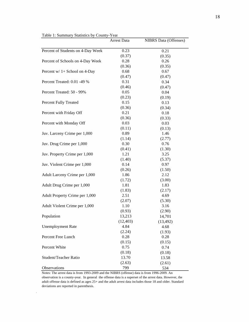
for the entire sample, 1993 through 2009. Summary statistics are reported in Table 1 (column 1).

This dataset has the advantage of covering all arrests in Colorado. However, since it is aggregated

annually the timing does not match up perfectly with the treatment variable which is reported

by academic years. The second data source is the National Incident Based Reporting System

(NIBRS) program. NIBRS provides detailed information on reported crimes at the incident level,

6Less than 5% of the total student body in urban areas are affected by the policy compared to 20% in rural areas.Including urban counties in the analysis will introduce noise, which is generated by smaller changes in student popu-lation, into the treatment variable. We want our estimates to reflect changes due to policy adoption. That said, whilethere are some minor differences, the results are largely the same when urban counties are included.

7The MSAs omitted are Denver, Boulder, Greeley, Colorado Springs, Fort Collins, Pueblo, and Grand Junction.Other possible definitions of rural, such as population counts or only omitting the Denver MSA, have been consideredand have little influence on the estimated results.

8We thank Mark Anderson of Montana State University for helping us obtain this dataset.9While there is crime data available at more granular jurisdictional level than counties, these jurisdictions do not

overlap in any consistent way with school boundaries.10The results are similar if we use all students on a four-day school week regardless of age and percentage of schools

on a 4 day week.

8

including the date of the crime. This allows us to match the reported crimes with the treatment

variable by academic year and avoid a timing problem. Reported crimes are a superset of arrests

because they include people who are cited for a crime without actually being arrested, which is a

common occurrence. The number of offenses is aggregated to the county level to match the level

of treatment and the other dataset.

In addition to providing detailed data on individual crimes, an advantage of the NIBRS data

is that it flags the exact date of the offense and includes detailed demographic characteristics of

the offenders. This level of detail allows us to precisely identify juveniles in the sample as well

as examine changes in crime by day-of-the-week. Unfortunately, Colorado has only been fully

participating in the NIBRS program since 1997, so the data are not available for the entire sample

period. As such, all regressions using NIBRS data include the years 1997 through 2009. Addi-

tionally, while the data covers most of Colorado, there are some agencies (approximately 10% of

agencies covering approximately 10% of the state’s population) who do not participate in the pro-

gram, reducing the number of rural counties in the NIBRS sample to 43.11 Column 2 of Table 1

contains summary statistics for offenses from NIBRS.

The crime outcomes studied include property crimes, violent crimes, and drug violations. Prop-

erty crime is a general category consisting of larceny, breaking and entering, grand theft auto, and

arson. Violent crimes include homicide, sexual assault, robbery, and assault. Drug crimes are a

separate category. Some incidents reported in the NIBRS dataset involve more than one offense

(i.e. breaking and entering while in possession of illegal drugs). In these cases we count the inci-

dent in both categories. While this results in some double counting of incidents, the alternatives are

less palatable. Dropping all of these incidents results in a substantial loss of data. Some systems

use a hierarchy such that an incident is categorized as its most “severe” offense type; however,

these distinctions are often arbitrary and can result in under-counting of some kinds of crimes,

especially drug offenses.

11While we are able to adjust the sample by dropping agencies that do not fully participate in NIBRS, any remainingunderreporting should cause the coefficient to be biased downwards, as the number of reported crimes would be lowerthan actual number of crimes in the county.

9

4 Empirical Framework

We estimate the following difference-in-difference model

Yct = β0 +β1Tct +X ′ctα + γc +δt + εct (1)

where Yct is a count of crimes (arrests or offenses depending on the dataset) in county c and in

year t. Tct is the percent of students in a county-year that are on a four-day school week schedule,

and Xct is a vector of time varying county-year level covariates (unemployment, percent of students

in county eligible for free lunch, race, and student/teacher ratio). γc is a county level fixed effect,

δt is a year fixed effect to account for temporal changes in crime over the 16 year time horizon,

and εct is the usual error term. The treatment variable Tct is constructed by dividing the total

number of students in grades 6-12 in a county who are on the four-day week in a given year by the

total number of students in grades 6-12 in a county-year. We exclude summer months because no

students are treated during this time.

Given that crime (the outcome) is reported as a count, estimating the above model with a

standard Ordinary Least Squares approach is not appropriate as there is a large share of county-

year observations with a zero-count on juvenile crimes. That is, crime is positively skewed.12 In

fact, Ordinary Least Squares yields negative fitted values for 22% of the observations highlighting

the importance of a count model in this analysis. We instead estimate the model using Fixed-

Effects Poisson Quasi-Maximum Likelihood (QMLE); a model often used to accommodate count

data with an excess number of zeros (Hausman, Hall and Griliches (1984), Osgood (2000)).13 To

account for the fact that each county has a different population, and therefore a different potential

for crime, we include total population as the exposure variable in the Poisson regressions.14 Finally,

12Aggregating to the county-year-day of week level of crime, as we do in the second part of the analysis, onlyfurther exacerbates the issue of the high incidence of zero-count observations.

13Sometimes a log transformation is used when an outcome is positively skewed but, due to the large number ofzero-count crime observations, this approach is not sufficient.

14Although youth crime is a preferable exposure variable, due to the 10% of non-participating agencies in theNIBRS dataset we are not able to use it, instead the exposure variable is the population provided by NIBRS whichadjusts for the non-compliers. In order to make estimates comparable across datasets, total population in a count-yearis the exposure variable used with the arrest data as well. Note, we obtain similar results when we use youth populationas the exposure with the arrest data.

10

we report cluster-robust standard errors to account for overdispersion and within county correlation

of the dependent variable (Wooldridge (1999)).15

Anecdotally, there is little reason to believe that the adoption of the policy is in response to

crime patterns in a given county or correlated with unobservable time varying county characteris-

tics that also correlate with juvenile crime; two issues which would undermine the causal interpre-

tation of the policy’s effect. In Colorado, the schools that have adopted a four-day school week

most often cite financial savings as the reason (Grau and Shaughnessy, 1987; Donis-Keller and

Silvernail, 2009; Anderson and Walker, 2014). The Colorado Department of Education states that

four-day schedules are almost entirely adopted by schools in rural districts that serve a dispersed

group of students because they can save on transportation costs. Other reasons schools have de-

cided to switch include parent support, improved attendance, and increased academic performance.

We return to this issue in Section 6 and show that our results hold up to several placebo tests.

5 Results

5.1 County-Year

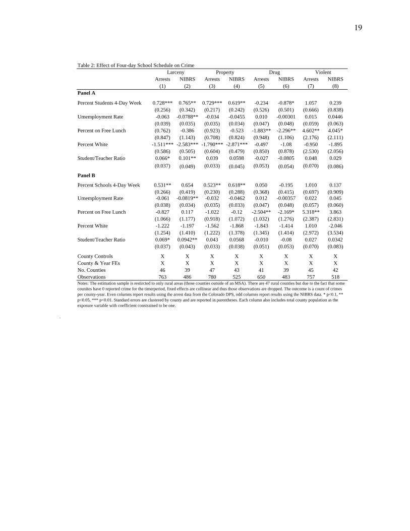
Table 2 reports regression coefficient estimates obtained from the arrest data in the odd num-

bered columns and results obtained from the reported offense data (NIBRS) in the even numbered

columns. Four crime outcomes (for both arrests and offenses) are included in each table: larceny,

property crime, drug violations and violent crime. Panel A reports results for a specification that

defines the treatment as the percent of students in a county-year who are on a four-day week while

Panel B reports results for an alternative way to define the treatment, the percent of schools in

a county-year who are on a four-day week schedule. The results in columns 1 and 2 – for both

Panel A and Panel B – show a significant increase in juvenile larceny arrests and offenses. A 10%

increase in the share of students in a county on a four-day week schedule leads to an increase in

15The QML estimator only restricts the within-county mean and variance to be equal, so a majority of the overdis-persion present in the juvenile crime data is accounted for without robust standard errors.

11

larceny crimes by about 7%.

Columns 3 and 4 report the estimated effect of the policy on all property crime. Since larceny

is part of property crime, it is not surprising that the effects are similar to the larceny estimates but

slightly smaller in magnitude. Students who have an additional day off during the week may be

more likely to engage in minor offenses such as shoplifting and other petty theft, while property

crimes such as arson and breaking and entering are less affected. The aggregation of all of these

crimes may account for the fact that property crime shows a somewhat smaller positive coefficient.

Finally, for both arrests and offenses the estimated effects of the percent of students on a four-day

school week on drug violations and violent crimes (columns 5-8) are, for the most part, statistically

insignificant. The varied findings across the different crime outcomes highlights the importance of

disaggregating by crime type. Uncovering how the policy affects each type of crime, if at all, and

through which channel helps provide a more comprehensive understanding of the impact of the

four-day school week schedule.

5.2 Day-of-the-Week

Aggregating NIBRS data to the day-of-the-week, county, year level allows one to examine the

effects of the four-day school week policy on specific days. Table 3 reports the corresponding

summary statistics for this level of aggregation. One reason to examine crime patterns at this finer

level is to learn more about the mechanism that underlies the main findings. Does crime increase on

all days of the week or specific days? A crime spike on Friday due to an increase in the number of

students who are treated on Friday would be consistent with the commonly accepted notion “ideal

hands are the devil’s workshop”. Put differently, students who are kept busy and supervised stay

out of trouble. If, however, crime is increasing on other days of the week as well, then likely there

are some spillover effects of the policy. Spillover effects may be particularly salient in our setting

given the distinct nature of the four-day week policy relative to other school schedule changes

used in the literature. Students on a four-day week schedule have an additional day-off per week

every week of the school year, as such, it is quite possible they are developing strong social groups

12

on this day – potentially carrying out devious behaviors together – which leads to gatherings and

devious behavior on other days of the week as well. Along these lines, because of the regular day

off associated with this policy, habit formation may play an important role; students may form poor

habits, either with a social group or individually, that carry-over to other days of the week.

To investigate this, we estimate the following model using Fixed-Effects Poisson QML:

Yctd = β0+β1T Fct +β2T Mct +7

∑d=1

θdT Fct ∗ψd +7

∑d=1

µdT Mct ∗ψd +X ′ctα+γc+δt +ψd +εctd (2)

where ψd is a set of dummy variables indicating the day of the week (Wednesday is the omitted

day). T Fct and T Mct are the percent of students in a county-year treated on Friday and Monday

respectively. Both treatment variables are also interacted with each day of the week which are

represented by the following vectors, ∑7d=1 θdT Fct ∗ψd and ∑

7d=1 µdT Mct ∗ψd . Other controls

included are defined in the previous section.

Table 4 presents the effect of having Friday off by day of the week.16 There appears to be no

evidence that crime differentially increases on a particular day. The policy does not cause crime to

increase on Friday (the day students have off) any more than any other day of the week. Instead,

youth larceny and property crimes appear to be higher as a result of having Friday off on all days of

the week. One possible explanation for this result is that because we are analyzing rural counties,

there are too few observations in a given county/year/day cell to detect any differences across days.

Another explanation is that students who have an “extra” day off per week not only increase their

unlawful behavior on their day off, but this also spills over to other days of the week. Similar to

the county-year results in Table 2, we find no consistent changes in drug or violent crimes due to

the policy, either overall or on any given day of the week.

6 Robustness Checks

The results reported so far are robust to alternative definitions of rural and are available upon

request. Two additional robustness checks – a robustness check using adult crime and a county-

16Appendix Table A1 reports the full set of point estimates for Equation 2.

13

year placebo test – are examined in this section.

To ensure that the treatment variable is not picking up some underlying change, such as changes

in the local economy or law enforcement practices, we run identical models using adult (age 25+)

crime as the outcome.17 If juvenile crime is only increasing in areas because of the treatment (the

four-day week policy), then the relationship between the percent of juveniles on a four-day week

in a given county-year and adult crimes should not be statistically different from zero. Table 5,

which is formatted the same as Table 2, contains the results for adult arrests and adult offenses at

the county-year level. Neither dataset (arrests or offenses) indicates a significant effect for adult

crime, supporting the idea that a four-day school week policy is uniquely impacting juveniles and

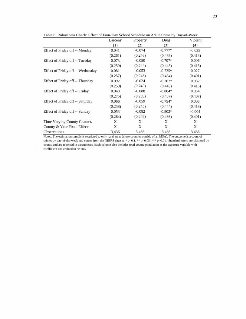
is not a proxy for other unobserved changes in the county. Table 6 reports results for adult crime by

day-of-week. While there appears to be no effect of the policy on adult larceny, property crimes,

or violent crimes, there is some evidence (statistically significant at the 10% level) that adult drug

crimes decrease. 18

Ideally, we would like to provide a standard event study that often accompanies a difference-

in-difference estimation strategy as another way to check for exogeneity of the treatment. However

given the structure of the policy and the availability of crime data, this setting does not lend itself

to this type of analysis. First, since crime data in Colorado are only available starting in 1993, and

schools started adopting the four-day week in the 1970s, we do not have a pretreatment period for a

majority of the treated counties. Additionally, treatment intensity can increase over time; the share

of students in a county who are treated can and does increase over the sample period for many of

the counties.

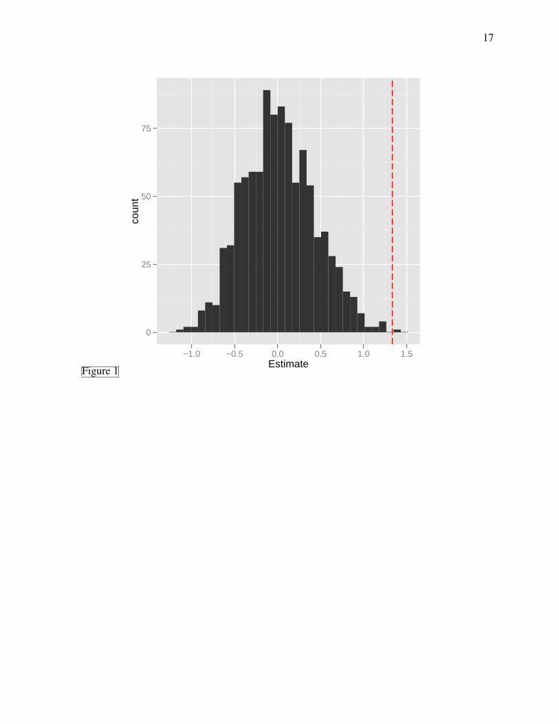
Instead, as an additional sensitivity test we conduct a county level placebo analysis. Coun-

ties are randomly reassigned the percent on a four-day week (the treatment variable) of a different

county. This reassignment maintains the characteristics of the treatment profile, the treatment turns

on and can increase over time, but the timing of treatment has been randomly reassigned. If our

17Individuals ages 18-25 are left out of these models. Some 18 year-olds are still in high school (and are thereforein the treated population) and those just out of high school are likely to socialize with treated individuals and may beindirectly affected by treatment.

18Table A2 reports the full set of estimates for adults by day-of-week.

14

main results are really capturing the effect of the policy on crime, the results for this specifica-

tion should reveal no relationship between the treatment and crime outcome since the reassigned

treatment does not reflect the true percent in that county-year who are treated. Figure 1 shows

the distribution of the estimated coefficients of the treatment variable from estimating Equation 1

1,000 times, each time with random reassignment of the treatment profile. The actual estimate is

indicated with a red dashed line. The median estimate of the effect and the associated statistics are

both essentially 0, which strongly suggests our observed effect is not an artifact of the estimation

strategy.

7 Discussion and Conclusion

In this paper we show that the implementation of the four-day school week in rural areas leads

to an increase in youth property crime, particularly larceny, while drug and violent crimes appear

unaffected. The property and larceny results are qualitatively similar to those found in Jacob

and Lefgren (2003) and Luallen (2006) but are somewhat larger. This difference is unsurprising

given that the variation in school schedule exploited in this setting is more frequent and permanent

than that in previous work, giving the treated students more “time off”. Moreover, unlike the

previous two studies, we do not find any effects of school on short-term violent crime. Again

differences in the findings across these studies are largely attributable to differences in the settings

studied. As stated by the United States Department of Justice, violent crime rates are much higher

in urban areas and both Jacob and Lefgren (2003) and Luallen (2006) rely on data from more urban

settings. Overall, these results are informative in that they highlight the fact that policymakers

should consider the unintended consequences before implementing such a schedule.

15

ReferencesAkee, Randall Q, Timothy J Halliday, and Sally Kwak, “Investigating the Effects of Furlough-

ing Public School Teachers on Juvenile Crime in Hawaii,” Economics of Education Review,2014, 42, 1–11.

Anderson, D Mark, “In school and out of trouble? The minimum dropout age and juvenile crime,”Review of Economics and Statistics, 2014, 96 (2), 318–331.

Anderson, Mark and Mary Beth Walker, “Does Shortening the School Week Impact StudentPerformance? Evidence from the Four-Day School Week,” Education Finance and Policy, 2014.

Berthelon, Matias E and Diana I Kruger, “Risky behavior among youth: Incapacitation effectsof school on adolescent motherhood and crime in Chile,” Journal of Public Economics, 2011,95 (1), 41–53.

Cross, Amanda Brown, Denise C Gottfredson, Denise M Wilson, Melissa Rorie, and NadineConnell, “The impact of after-school programs on the routine activities of middle-school stu-dents: Results from a randomized, controlled trial*,” Criminology & Public Policy, 2009, 8 (2),391–412.

Donis-Keller, Christine and David L Silvernail, Research brief: A review of the evidence on thefour-day school week, Center for Education Policy, Applied Research and Evaluation, Universityof Southern Maine, 2009.

Grau, Elnabeth and Michael F Shaughnessy, “The Four Day School Week: An Investigationand Analysis,” 1987.

Griffith, Michael, “What Savings Are Produced by Moving to a Four-Day School Week?,” Edu-cation Commission of the States (NJ3), 2011.

Hausman, Jerry A, Bronwyn H Hall, and Zvi Griliches, “Econometric models for count datawith an application to the patents-R&D relationship,” 1984.

Herring, Chris, “School’s New Math: The Four-Day Week,” Wall Street Journal, 2010.

Jacob, Brian A and Lars Lefgren, “Are Idle Hands the Devil’s Workshop? Incapacitation, Con-centration, and Juvenile Crime,” American Economic Review, 2003, 93 (5), 1560–1577.

Kingsbury, Kathleen, “Four-Day School Weeks,” TIMES, 2008.

Lochner, Lance, “Education, Work, and Crime: A Human Capital Approach*,” InternationalEconomic Review, 2004, 45 (3), 811–843.

, “Education policy and crime,” in “Controlling crime: strategies and tradeoffs,” University ofChicago Press, 2010, pp. 465–515.

and Enrico Moretti, “The Effect of Education on Crime: Evidence from Prison Inmates,Arrests, and Self-Reports,” The American Economic Review, 2004, 94 (1), 155–189.

16

Luallen, Jeremy, “School’s out... forever: A study of juvenile crime, at-risk youths and teacherstrikes,” Journal of urban economics, 2006, 59 (1), 75–103.

Osgood, D Wayne, “Poisson-based regression analysis of aggregate crime rates,” Journal of quan-titative criminology, 2000, 16 (1), 21–43.

Rodríguez-Planas, Núria, “School and drugs: Closing the gap-Evidence from a randomized trialin the US,” Technical Report, Discussion Paper series, Forschungsinstitut zur Zukunft der Arbeit2012.

Snyder, Howard N and Melissa Sickmund, “Juvenile offenders and victims: 2006 national re-port.,” Office of juvenile justice and delinquency prevention, 2006.

Wooldridge, Jeffrey M, “Distribution-free estimation of some nonlinear panel data models,” Jour-nal of Econometrics, 1999, 90 (1), 77–97.

17

Figure 1

0

25

50

75

−1.0 −0.5 0.0 0.5 1.0 1.5Estimate

coun

t

18

Arrest Data NIBRS Data (Offenses)

Percent of Students on 4-Day Week 0.23 0.21(0.37) (0.35)

Percent of Schools on 4-Day Week 0.28 0.26(0.36) (0.35)

Percent w/ 1+ School on 4-Day 0.68 0.67(0.47) (0.47)

Percent Treated: 0.01 -49 % 0.31 0.34(0.46) (0.47)

Percent Treated: 50 - 99% 0.05 0.04(0.23) (0.19)

Percent Fully Treated 0.15 0.13(0.36) (0.34)

Percent with Friday Off 0.21 0.18(0.36) (0.33)

Percent with Monday Off 0.03 0.03(0.11) (0.13)

Juv. Larceny Crime per 1,000 0.89 1.46(1.14) (2.77)

Juv. Drug Crime per 1,000 0.30 0.76(0.41) (1.30)

Juv. Property Crime per 1,000 1.21 3.25(1.40) (5.37)

Juv. Violent Crime per 1,000 0.14 0.97(0.26) (1.50)

Adult Larceny Crime per 1,000 1.86 2.12(1.72) (3.00)

Adult Drug Crime per 1,000 1.81 1.83(1.83) (2.17)

Adult Property Crime per 1,000 2.51 4.69(2.07) (5.30)

Adult Violent Crime per 1,000 1.10 3.16(0.93) (2.90)

Population 13,213 14,701(12,403) (13,492)

Unemployment Rate 4.84 4.68(2.24) (1.93)

Percent Free Lunch 0.28 0.28(0.15) (0.15)

Percent White 0.75 0.74(0.18) (0.18)

Student/Teacher Ratio 13.70 13.58(2.63) (2.61)

Observations 799 534

Table 1: Summary Statistics by County-Year

Notes: The arrest data is from 1993-2009 and the NIBRS (offense) data is from 1996-2009. An observation is a county-year. In general the offense data is a superset of the arrest data. However, the adult offense data is defined as ages 25+ and the adult arrest data includes those 18 and older. Standard deviations are reported in parenthesis.

19

Arrests NIBRS Arrests NIBRS Arrests NIBRS Arrests NIBRS(1) (2) (3) (4) (5) (6) (7) (8)

Panel A

Percent Students 4-Day Week 0.728*** 0.765** 0.729*** 0.619** -0.234 -0.878* 1.057 0.239(0.256) (0.342) (0.217) (0.242) (0.526) (0.501) (0.666) (0.838)

Umemployment Rate -0.063 -0.0788** -0.034 -0.0455 0.010 -0.00301 0.015 0.0446(0.039) (0.035) (0.035) (0.034) (0.047) (0.048) (0.059) (0.063)

Percent on Free Lunch (0.762) -0.386 (0.923) -0.523 -1.883** -2.296** 4.602** 4.045*(0.847) (1.143) (0.708) (0.824) (0.948) (1.106) (2.176) (2.111)

Percent White -1.511*** -2.583*** -1.790*** -2.871*** -0.497 -1.08 -0.950 -1.895(0.586) (0.505) (0.604) (0.479) (0.850) (0.878) (2.530) (2.056)

Student/Teacher Ratio 0.066* 0.101** 0.039 0.0598 -0.027 -0.0805 0.048 0.029(0.037) (0.049) (0.033) (0.045) (0.053) (0.054) (0.070) (0.086)

Panel B

Percent Schools 4-Day Week 0.531** 0.654 0.523** 0.618** 0.050 -0.195 1.010 0.137(0.266) (0.419) (0.230) (0.288) (0.368) (0.415) (0.697) (0.909)

Umemployment Rate -0.061 -0.0819** -0.032 -0.0462 0.012 -0.00357 0.022 0.045(0.038) (0.034) (0.035) (0.033) (0.047) (0.048) (0.057) (0.060)

Percent on Free Lunch -0.827 0.117 -1.022 -0.12 -2.504** -2.169* 5.318** 3.863(1.066) (1.177) (0.918) (1.072) (1.032) (1.276) (2.387) (2.831)

Percent White -1.222 -1.197 -1.562 -1.868 -1.843 -1.414 1.010 -2.046(1.254) (1.410) (1.222) (1.378) (1.345) (1.414) (2.972) (3.534)

Student/Teacher Ratio 0.069* 0.0942** 0.043 0.0568 -0.010 -0.08 0.027 0.0342(0.037) (0.043) (0.033) (0.038) (0.051) (0.053) (0.070) (0.083)

County Controls X X X X X X X XCounty & Year FEs X X X X X X X XNo. Counties 46 39 47 43 41 39 45 42Observations 763 486 780 525 650 483 757 518

Table 2: Effect of Four-day School Schedule on Crime

Notes: The estimation sample is restircted to only rural areas (those counties outside of an MSA). There are 47 rural counties but due to the fact that some counites have 0 reported crime for the timerperiod, fixed effects are collinear and thus those observations are dropped. The outcome is a count of crimes per county-year. Even columns report results using the arrest data from the Colorado DPS, odd columns report results using the NIBRS data. * p<0.1, ** p<0.05, *** p<0.01. Standard errors are clustered by county and are reported in parentheses. Each column also includes total county population as the exposure variable with coefficient constrained to be one.

Larceny Property Drug Violent

20

No Treat Off Fri Off Mon No Treat Off Fri Off Mon No Treat Off Fri Off Mon No Treat Off Fri Off Mon

Overall Crime 0.19 0.14 0.14 0.40 0.29 0.32 0.12 0.08 0.06 0.12 0.11 0.10(0.519) (0.299) (0.333) (0.898) (0.551) (0.542) (0.372) (0.247) (0.128) (0.320) (0.220) (0.203)

Observations 1,688 1,094 440 1,688 1,094 440 1,688 1,094 440 1,688 1,094 440

Monday 0.22 0.12 0.11 0.45 0.24 0.26 0.09 0.07 0.05 0.11 0.10 0.11(0.689) (0.219) (0.242) (0.998) (0.414) (0.457) (0.221) (0.158) (0.109) (0.311) (0.143) (0.178)

Tuesday 0.21 0.16 0.15 0.37 0.30 0.36 0.14 0.09 0.06 0.15 0.14 0.095(0.819) (0.341) (0.354) (0.941) (0.545) (0.651) (0.475) (0.164) (0.117) (0.347) (0.263) (0.179)

Wednesday 0.20 0.14 0.16 0.40 0.27 0.29 0.12 0.11 0.08 0.12 0.11 0.10(0.431) (0.278) (0.394) (0.793) (0.442) (0.529) (0.361) (0.343) (0.164) (0.278) (0.252) (0.153)

Thursday 0.18 0.11 0.14 0.33 0.27 0.29 0.11 0.08 0.07 0.13 0.13 0.10(0.409) (0.194) (0.291) (0.568) (0.449) (0.495) (0.312) (0.177) (0.143) (0.407) (0.235) (0.214)

Friday 0.22 0.18 0.19 0.52 0.34 0.46 0.17 0.07 0.05 0.18 0.13 0.09(0.420) (0.355) (0.440) (1.398) (0.711) (0.639) (0.563) (0.126) (0.093) (0.412) (0.265) (0.162)

Saturday 0.17 0.16 0.11 0.39 0.33 0.29 0.10 0.11 0.05 0.08 0.10 0.09(0.340) (0.405) (0.299) (0.672) (0.671) (0.483) (0.293) (0.387) (0.168) (0.222) (0.187) (0.216)

Sunday 0.13 0.09 0.11 0.32 0.27 0.26 0.06 0.06 0.02 0.07 0.09 0.10(0.320) (0.229) (0.277) (0.618) (0.552) (0.496) (0.243) (0.241) (0.052) (0.185) (0.160) (0.292)

Notes: The sample is restircted to only rural areas (those counties outside of an MSA). Crime is reported as offenses per 1,000 population. We exclude summer months. Standard deviations are reprted in parenthesis.

Table 3: Summary Stats by Day-of-Week (NIBRS Offense Data) Larceny Property Drug Violent

Larceny Property Drug Violent(1) (2) (3) (4)

Effect of Friday off -- Monday 0.870** 0.799*** -0.824 0.541(0.346) (0.222) (0.549) (0.797)

Effect of Friday off -- Tuesday 0.864** 0.842*** -0.805 0.625(0.347) (0.224) (0.559) (0.796)

Effect of Friday off -- Wednesday 0.917*** 0.854*** -0.867 0.626(0.314) (0.215) (0.555) (0.814)

Effect of Friday off -- Thursday 0.893*** 0.876*** -0.807 0.602(0.345) (0.224) (0.561) (0.794)

Effect of Friday off -- Friday 0.865*** 0.819*** -0.841 0.508(0.310) (0.219) (0.557) (0.816)

Effect of Friday off -- Saturday 0.876** 0.847*** -0.805 0.615(0.347) (0.224) (0.557) (0.806)

Effect of Friday off -- Sunday 0.900*** 0.847*** -0.854 0.556(0.316) (0.217) (0.557) (0.802)

Time Varying County Charact. X X X XCounty & Year Fixed Effects X X X XObservations 3,216 3,414 3,222 3,369

Table 4: Effect of Four-Day School Schedule on Crime by Day-of-Week

Notes: The estimation sample is restricted to only rural areas (those counties outside of an MSA). The outcome is a count of crimes by day-of-the-week and comes from the NIBRS dataset. * p<0.1, ** p<0.05, *** p<0.01. Standard errors are clustered by county and are reported in parentheses. Each column also includes total county population as the exposure variable with coefficient constrained to be one.

21

Arrests NIBRS Arrests NIBRS Arrests NIBRS(1) (2) (3) (4) (5) (6)

Panel A

Percent Students 4-Day Week 0.122 -0.199 0.057 -0.223 -0.238 -0.544(0.162) (0.273) (0.158) (0.250) (0.468) (0.428)

Umemployment Rate -0.026 -0.0446 -0.041 -0.0447 -0.026 -0.0398(0.037) (0.037) (0.036) (0.034) (0.045) (0.045)

Percent on Free Lunch -0.678 -1.42 -0.648 -1.376 -0.136 -0.178(1.045) (1.425) (1.006) (1.289) (1.025) (1.094)

Percent White 1.210* 0.24 0.668 -0.0416 1.728* 1.006(0.663) (0.818) (0.674) (0.822) (0.888) (0.670)

Student/Teacher Ratio -0.001 -0.0137 0.001 -0.0309 0.015 -0.0246(0.031) (0.042) (0.028) (0.037) (0.030) (0.036)

Panel B

Percent Schools 4-Day Week 0.164 -0.272 0.103 -0.245 -0.307 -0.288(0.224) (0.372) (0.203) (0.311) (0.383) (0.311)

Umemployment Rate -0.025 -0.044 -0.040 -0.0447 -0.024 -0.0378(0.037) (0.038) (0.036) (0.035) (0.045) (0.045)

Percent on Free Lunch -0.577 -0.635 -0.335 -0.759 -1.099 -0.722(1.391) (1.728) (1.296) (1.594) (1.229) (1.427)

Percent White 1.431 1.728 1.224 1.085 -0.255 -0.383(1.340) (1.536) (1.231) (1.486) (1.388) (1.584)

Student/Teacher Ratio -0.001 -0.0331 -0.003 -0.0455 0.029 -0.012(0.028) (0.035) (0.026) (0.031) (0.030) (0.034)

County Controls X X X X X XCounty & Year FEs X X X X X XNo. Counties 47 44 47 44 47 44Observations 780 534 780 534 780 534Notes: The estimation sample is restircted to only rural areas (those counties outside of an MSA). There are 47 rural counties butcounites have 0 reported crime for the timerperiod, fixed effects are collinear and thus those observations are dropped. The outcocounty-year. Even columns report results using the arrest data from the Colorado DPS, odd columns report results using the NIBp<0.05, *** p<0.01. Standard errors are clustered by county and are reported in parentheses. Each column also includes total couexposure variable with coefficient constrained to be one.

Table 5: Robustness Check -- Effect of Four-Day School Schedule on Adult Crime Larceny Property Drug

22

Larceny Property Drug Violent(1) (2) (3) (4)

Effect of Friday off -- Monday 0.041 -0.074 -0.777* -0.035(0.261) (0.246) (0.439) (0.413)

Effect of Friday off -- Tuesday 0.073 -0.050 -0.797* 0.006(0.259) (0.244) (0.445) (0.415)

Effect of Friday off -- Wednesday 0.081 -0.053 -0.735* 0.027(0.257) (0.243) (0.434) (0.401)

Effect of Friday off -- Thursday 0.092 -0.024 -0.767* 0.032(0.259) (0.245) (0.445) (0.416)

Effect of Friday off -- Friday 0.048 -0.088 -0.804* 0.054(0.275) (0.259) (0.437) (0.407)

Effect of Friday off -- Saturday 0.066 -0.059 -0.754* 0.005(0.258) (0.245) (0.444) (0.418)

Effect of Friday off -- Sunday 0.053 -0.082 -0.802* -0.004(0.264) (0.249) (0.436) (0.401)

Time Varying County Charact. X X X XCounty & Year Fixed Effects X X X XObservations 3,436 3,436 3,436 3,436

Table 6: Robustness Check: Effect of Four-Day School Schedule on Adult Crime by Day-of-Week

Notes: The estimation sample is restricted to only rural areas (those counties outside of an MSA). The outcome is a count of crimes by day-of-the-week and comes from the NIBRS dataset. * p<0.1, ** p<0.05, *** p<0.01. Standard errors are clustered by county and are reported in parentheses. Each column also includes total county population as the exposure variable with coefficient constrained to be one.

23

Larceny Property Drug Violent(1) (2) (3) (4)

Percent Treated Friday 0.917*** 0.854*** -0.867 0.626(0.314) (0.215) (0.555) (0.814)

Percent Treated Monday 0.076 -0.510 -1.500 -0.284(2.083) (0.756) (1.245) (1.550)

Percent Treated Fri X Fri -0.052** -0.035 0.026 -0.118(0.026) (0.040) (0.028) (0.141)

Percent Treated Fri X Sat -0.041 -0.008 0.062** -0.011(0.059) (0.054) (0.029) (0.050)

Percent Treated Fri X Sun -0.021 -0.007 0.013 -0.070(0.014) (0.014) (0.027) (0.061)

Percent Treated Fri X Mon -0.047 -0.056 0.0429* -0.085(0.054) (0.050) (0.025) (0.107)

Percent Treated Fri X Tues -0.053 -0.012 0.062*** -0.001(0.059) (0.053) (0.019) (0.047)

Percent Treated Fri X Thurs -0.024 0.022 0.061 -0.024(0.060) (0.056) (0.038) (0.073)

Percent Treated Mon X Fri -0.042 0.027 0.106 0.033(0.131) (0.099) (0.109) (0.145)

Percent Treated Mon X Sat -0.089 -0.130 -0.119* -0.186(0.126) (0.099) (0.062) (0.130)

Percent Treated Mon X Sun 0.080 0.072 0.096 -0.095(0.212) (0.158) (0.088) (0.197)

Percent Treated Mon X Mon -0.019 -0.046 -0.069 0.041(0.129) (0.101) (0.046) (0.100)

Percent Treated Mon X Tues 0.100 0.148 0.081 -0.185(0.167) (0.101) (0.116) (0.251)

Percent Treated Mon X Thurs 0.146 0.152 -0.022 -0.097(0.178) (0.126) (0.053) (0.192)

Monday 0.005 0.004 -0.003 -0.004(0.004) (0.003) (0.003) (0.007)

Tuesday 0.004 0.002 -0.004 -0.003(0.004) (0.003) (0.003) (0.005)

Tursday -0.002 -0.004 -0.002 -0.011(0.003) (0.003) (0.002) (0.013)

Friday 0.012 0.007 -0.005 0.004(0.009) (0.006) (0.007) (0.010)

Saturday 0.005 0.004 0.003 0.004(0.004) (0.004) (0.004) (0.005)

Sunday 0.004 0.003 -0.001 0.002(0.004) (0.003) (0.003) (0.006)

Time Varying County Charact. X X X XCounty & Year Fixed Effects X X X XObservations 3,216 3,414 3,222 3,369Notes: The estimation sample is restricted to only rural areas (those counties outside of an MSA). The outcome is a count of crimes by day-of-the-week . * p<0.1, ** p<0.05, *** p<0.01. Standard errors are clustered by county and are reported in parentheses. Each column also includes total county population as the exposure variable with coefficient constrained to be one.

Table A1: Effect of Four-Day School Schedule on Crime (NIBRS Data)

24

Larceny Property Drug Violent(1) (2) (3) (4)

Percent Treated Friday 0.081 -0.053 -0.735* 0.027(0.257) (0.243) (0.434) (0.401)

Percent Treated Monday -0.301 0.692 1.410*** 0.543(0.981) (0.470) (0.460) (0.879)

Percent Treated Fri X Fri -0.033 -0.035 -0.069 0.027(0.034) (0.029) (0.059) (0.035)

Percent Treated Fri X Sat -0.015 -0.007 -0.019 -0.022(0.032) (0.026) (0.030) (0.046)

Percent Treated Fri X Sun -0.028 -0.029 -0.067 -0.031(0.025) (0.030) (0.052) (0.027)

Percent Treated Fri X Mon -0.040 -0.022 -0.042 -0.062(0.031) (0.027) (0.028) (0.064)

Percent Treated Fri X Tues -0.008 0.003 -0.062 -0.021(0.030) (0.025) (0.056) (0.033)

Percent Treated Fri X Thurs 0.012 0.029 -0.032 0.005(0.034) (0.036) (0.041) (0.044)

Percent Treated Mon X Fri 0.159 0.167 -0.038 0.311(0.233) (0.149) (0.129) (0.191)

Percent Treated Mon X Sat 0.127 -0.027 -0.339*** 0.199(0.201) (0.062) (0.117) (0.240)

Percent Treated Mon X Sun 0.159 0.192 -0.313* 0.570(0.305) (0.330) (0.169) (0.368)

Percent Treated Mon X Mon 0.169 0.009 -0.327*** 0.293(0.194) (0.052) (0.125) (0.218)

Percent Treated Mon X Tues 0.029 -0.033 -0.300** 0.412**(0.114) (0.100) (0.119) (0.199)

Percent Treated Mon X Thurs 0.217 0.199 -0.120 0.492(0.258) (0.243) (0.084) (0.315)

Monday 0.006 0.006 0.001 0.005(0.006) (0.005) (0.002) (0.004)

Tuesday 0.005 0.005 0.003 -0.001(0.006) (0.005) (0.002) (0.004)

Tursday -0.002 -0.003 0.001 -0.005(0.003) (0.003) (0.002) (0.004)

Friday 0.008 0.005 -0.003 -0.005(0.009) (0.007) (0.004) (0.008)

Saturday 0.003 0.004 0.001 0.003(0.005) (0.005) (0.002) (0.004)

Sunday 0.006 0.006 0.005 0.003(0.006) (0.005) (0.003) (0.004)

Time Varying County Charact. X X X XCounty & Year Fixed Effects X X X XObservations 3,436 3,436 3,436 3,436

Table A2: Effect of Four-Day School Schedule on Adult Crime (NIBRS Data)

Notes: The estimation sample is restricted to only rural areas (those counties outside of an MSA). The outcome is a count of crimes by day-of-the-week . * p<0.1, ** p<0.05, *** p<0.01. Standard errors are clustered by county and are reported in parentheses. Each column also includes total county population as the exposure variable with coefficient constrained to be one.