jwuk rnc 1577 - stanford universityboyd/papers/pdf/contr_coef_trunc.pdf · the complexity of a...

INTERNATIONAL JOURNAL OF ROBUST AND NONLINEAR CONTROLInt. J. Robust. Nonlinear Control (2010)Published online in Wiley InterScience (www.interscience.wiley.com). DOI: 10.1002/rnc.1577

Controller coefficient truncation using Lyapunovperformance certificate

Joëlle Skaf and Stephen P. Boyd!,†

Information Systems Laboratory, Department of Electrical Engineering, Stanford University,Stanford, CA 94305, U.S.A.

SUMMARY

We describe a method for truncating the coefficients of a linear controller while guaranteeing that a givenset of relaxed performance constraints is met. Our method sequentially and greedily truncates individualcoefficients, using a Lyapunov certificate, typically in linear matrix inequality (LMI) form, to guaranteethe performance. Numerical examples show that the method is surprisingly effective at finding controllerswith aggressively truncated coefficients, which meet typical performance constraints. We give an exampleshowing that how the basic method can be extended to handle nonlinear plants and controllers. Copyright! 2010 John Wiley & Sons, Ltd.

Received 5 March 2009; Revised 29 October 2009; Accepted 18 January 2010

KEY WORDS: coefficient truncation; controller design; LMI methods

1. INTRODUCTION

1.1. The controller coefficient truncation problem

We consider a discrete-time linear time-invariant control system, with plant

xp(t+1)= Apxp(t)+B1w(t)+B2u(t),

z(t)= C1xp(t)+D11w(t)+D12u(t),

y(t)= C2xp(t)+D21w(t),

and controller

xc(t+1)= Acxc(t)+Bcy(t),

u(t)= Ccxc(t)+Dcy(t).

!Correspondence to: Stephen P. Boyd, Information Systems Laboratory, Department of Electrical Engineering, StanfordUniversity, Stanford, CA 94305, U.S.A.

†E-mail: [email protected]

Contract/grant sponsor: Focus Center Research Program Center for Circuit and System Solutions (www.c2s2.org);contract/grant number: 2003-CT-888Contract/grant sponsor: AFOSR; contract/grant number: AF F49620-01-1-0365Contract/grant sponsor: NSF; contract/grant number: ECS-0423905Contract/grant sponsor: NSF; contract/grant number: 0529426Contract/grant sponsor: DARPA/MIT; contract/grant number: 5710001848Contract/grant sponsor: AFOSR; contract/grant number: FA9550-06-1-0514Contract/grant sponsor: DARPA/Lockheed; contract/grant number: N66001-06-C-2021Contract/grant sponsor: AFOSR/Vanderbilt; contract/grant number: FA9550-06-1-0312

Copyright ! 2010 John Wiley & Sons, Ltd.

J. SKAF AND S. P. BOYD

Here xp(t) is the plant state, u(t) is the control input, y(t) is the sensor output, w(t) and z(t) arethe exogenous input and output, respectively, and xc(t) is the controller state.

The vector !"RN will represent the design parameters or coefficients in the controller. Typicallythese are (some of) the entries in the matrices Ac, Bc, Cc, and Dc. We are given a nominal controllerdesign, described by the coefficient vector !nom, and a set of acceptable controller designs C#RN .The setC gives the (coefficients of the) controllers that achieve acceptable closed-loop performance.We assume that !nom"C, i.e. the nominal controller meets the performance specifications. Forexample, we can give C in terms of a single scalar performance measure J :RN $R, as

C={!|J (!)!(1+")J (!nom)},

which are the designs no more than " worse than the nominal. If the nominal design is the controllerthat minimizes J , then C is the set of "-suboptimal designs. Our goal is to find !"C that achievesclosed-loop performance close to the nominal, and at the same time low complexity.

The complexity of a vector of controller coefficients ! is measured by the function ! :RN $R,

!(!)=N!i=1

#i (!i ),

where #i (!i ) gives the complexity of the i th coefficient of !. We can take, for example, #i (a) tobe the number of bits needed to express a, or the total number of 1s in the binary expansion of a,in which case !(!) gives the total number of bits (or 1s) in the controller coefficients. Of coursethe functions #i , and therefore also !, can be discontinuous.

Our goal is to find the lowest complexity controller among the acceptable designs. We canexpress this as the optimization problem

minimize !(!)

subject to !"C,(1)

with variable !"RN . We call this as the controller coefficient truncation problem (CCTP), sincewe can think of the controller coefficient !i as a truncated version of the nominal controllercoefficient !nomi .

The CCTP (1) is in general very difficult to solve. For example, when ! measures bit complexity,the CCTP can be cast as a combinatorial optimization problem, with the binary expansions ofthe coefficients as Boolean (i.e. {0,1}) variables. Branch-and-bound, or other global optimizationtechniques, can be used to solve small CCTPs, with perhaps 10 coefficients. But we are interestedin methods that can handle much larger problems, with perhaps hundreds (or more) of controllercoefficients. In addition, it is not crucial to find the global solution of the CCTP (1); it is enoughto find a controller with low (if not lowest) complexity.

In this paper we describe a heuristic algorithm for the CCTP (1) that runs quickly and scalesto large problems. While the designs produced are very likely not globally optimal, they appearto be quite good. The method typically produces aggressively truncated controller designs, evenwhen the allowed performance degradation over the nominal design is just a few per cent.

In our method, we greedily truncate individual coefficients sequentially, in random order, usinga Lyapunov certificate (which is updated at each step) to guarantee the performance, i.e. !"C.When the algorithm is run multiple times, the randomness in the truncation order produces designsthat are different, but have very similar total complexity. Running the algorithm a few times, andtaking the best controller found, can give a modest improvement over running it just once.

Before proceeding we mention a related issue that we do not consider, at least until Section 6:the effects of truncation or saturation of the control signals u(t), y(t), and xc(t). This makes theentire control system nonlinear, and can lead to instability, large and small limit cycles, and otherbehavior. However, the Lyapunov-based methods described in the paper can be extended to handlenonlinearities; we briefly describe one such extension in Section 6.

Copyright ! 2010 John Wiley & Sons, Ltd. Int. J. Robust. Nonlinear Control (2010)DOI: 10.1002/rnc

CONTROLLER COEFFICIENT TRUNCATION

1.2. Previous and related work

The subject of coefficient truncation is relatively old. It was initially discussed in the context offilter design: there was an understandable interest in designing finite word-length filters that wouldbe easily implemented in hardware with a small degradation in performance (see [1, 2]). The ideaof coefficient truncation subsequently appeared in other fields, such as speech processing [3] andcontrol [4].

Several methods have been proposed for coefficient truncation: exhaustive search over possibletruncated coefficients [1], successive truncation of coefficients and re-optimization over remainingones [2, 5], local bivariate search around the scaled and truncated coefficients [6], tree-traversaltechniques for truncated coefficients organized in a tree according to their complexity [7, 8], coef-ficient quantization using information-theoretic bounds [9], weighted least squares [10], simulatedannealing [11, 12], genetic algorithms [13, 14], Tabu search [15], and design of optimal filter realiza-tions that minimize coefficient complexity [11, 16]. Other approaches have formulated the problemas a nonlinear discrete optimization problem [17], or have used integer programming techniquesover the space of powers-of-two coefficients [18, 19]. Barua et al. [20] surveys different methodsfor quantizing lifting coefficients for wavelet filters: mostly uniform bit allocation, exhaustivelysearched allocation, and simulated annealing with lumped scaling and/or gain compensation. Liuet al. [21] presents how to choose the optimal realization for an Linear Quadratic Gaussian (LQG)controller to be robust to finite word-length effects. The effects of quantization and finite wordlength on robust stability of digital controllers and performance bounds derived using Lyapunovtheory are presented in [22].

1.3. Outline

In Section 2 we describe the general algorithm. In the next three sections we present examples,in each case working out the details for the general case, and illustrating the algorithm with anumerical instance of the problem. In Section 3 the controller has constant state feedback form, thenominal controller is linear quadratic regular (LQR) optimal, and the set of acceptable controllersis determined by the LQR cost. In Section 4 the controller is dynamic, and the objective is thedecay rate of the closed-loop system. In Section 5 the controller is dynamic, with order equalto the plant; the nominal controller is a central H% optimal controller, and the set of acceptablecontrollers is determined by an H% criterion. In Section 6 we consider a simple example of anonlinear feedback system, consisting of a linear plant and a controller that is nominally linear,but includes saturation in the state update and output equations. The objective is the decay rate ofthe nonlinear system.

2. THE ALGORITHM

Our algorithm uses two subroutines or methods: interv, which finds an interval of acceptable valuesof a coefficient and trunc, which truncates a coefficient, given an interval of acceptable choices.We first describe these methods more precisely, but still abstractly; more concrete descriptions willbe given later in Sections 2.1 and 2.2.

The method interv(!, i) takes as input the coefficient vector !"C and a coefficient index i . Itreturns an interval [l,u] of allowed values for !i , with the other parameters held fixed, i.e. numbersl and u, with !i " [l,u], with

(!1, . . . ,!i&1, z,!i+1, . . . ,!N )"C for z" [l,u].

Of course the simple choice l=u=!i is always valid. At the other extreme, the largest validinterval that can be returned by interv is given by

l! = inf{l|(!1, . . . ,!i&1, z,!i+1, . . . ,!N )"C for z" [l,!i ]},

u! = sup{u|(!1, . . . ,!i&1, z,!i+1, . . . ,!N )"C for z" [!i ,u]}.



A typical implementation of interv falls between these two extremes, returning a reasonablylarge interval guaranteed to lie in C, with reasonable computational effort. In the examples wewill consider, this can be done using linear matrix inequalities (LMIs).

The trunci (x, l,u) is a truncation method which, given a number x to be truncated and aninterval [l,u] of acceptable choices (containing x), returns a number z in the interval [l,u] with!i (z)!!i (x). One valid choice is z= x ; at the other extreme, the algorithm can return the pointwith smallest complexity in the interval, i.e. the minimizer of !i (z) over [l,u]. For the complexitymeasures that we use in the examples shown later, we can easily compute the latter.

The algorithm is initialized with the nominal design, which we assume has finite complexity.At each step an index i is chosen, and all parameters except !i are fixed. We use interv to findan interval of acceptable values for !i , and then trunc to find a value of !i with (possibly) lowercomplexity. We have experimented with various methods for choosing the index i in each step, andfound the best results by organizing the algorithm into passes, each of which involves updatingeach parameter once; in each pass, the ordering of the indices is random. The algorithm stopswhen the parameter does not change over one pass. A high-level description of the algorithm ispresented next:

! :=!nom

repeat!prev :=!choose a permutation $ of (1, . . . ,N )for i =1 to N

j :=$(i)[l,u] := interv(!, j )! j := trunci (! j , l,u)

until !=!prev

As the algorithm is random, it can and does converge to different points in different runs. It canbe run several times, taking the best controller coefficient vector found as our final choice.

2.1. Complexity measures and truncation methods

In this section we describe various possible complexity measures and the associated truncationmethods. Any z"R can be written as

z= s%!

i=&%bi2&i ,

where s" {&1,1} is the sign and bi " {0,1} are the bits of z in a binary expansion. (This represen-tation can be made unique by ruling out any sequence that ends with all ones, i.e. bi =1 for i"k,for some k).

One possible complexity measure is the number of ones in the binary expansion of z,

#ones(z)=%!

i=&%bi ,

which gives the number of adders needed to implement multiplication by z using a shift and summethod.

Another complexity measure is the width of the range of the non-zero bits, more commonlyreferred to as the number of bits in the expansion of z,

#bits(z)=max{i |bi '=0}&min{i |bi '=0}+1.

This measure is useful if multiplication by z will be carried out in fixed-point arithmetic.Yet another complexity measure is the number of bits needed in the fractional part of the binary

expansion of z,

#frac-bits(z)=max"0,max

i{i |bi '=0}

#.



For these complexity measures, it is straightforward to find the number z that minimizes themeasure in a given interval, i.e. to implement (the most powerful) trunc method. We assume thatthe binary expansions of l and u are finite (though possibly long),

sll&L . . .l0.l1 . . . lR, suu&L . . .u0.u1 . . .uR,

respectively. The number z will have at most L bits in its integer part and R bits in its fractionalpart, and we denote its bits as

sz z&L . . . z0.z1 . . . zR .

With complexity measure #ones or #bits, z can be found as follows:

zi :=0 for all ifor i =&L to R

if li =ui , zi := lielseif all bits after li are 0, breakelse zi :=1

When the complexity measure is #frac-bits, the same algorithm can be used, with zi initially set tozero for i>0 and the for loop index modified to run from 1 to R, instead of from &L to R.

2.2. Interval computation via Lyapunov performance certificate

Our approach to determining an interval [l,u] for which

(!1, . . . ,!i&1, z,!i+1, . . . ,!N )"C for z" [l,u]

will be based on a conservative approximation of C. Given !"C we first find a convex set C thatsatisfies !" C and C#C. We then take

l = inf{z|(!1, . . . ,!i+1, z,!i+1, . . . ,!N )" C},

u = sup{z|(!1, . . . ,!i+1, z,!i+1, . . . ,!N )" C}.(2)

Since C is convex, it follows that

(!1, . . . ,!i+1, z,!i+1, . . . ,!N )" C#C for z" [l,u].

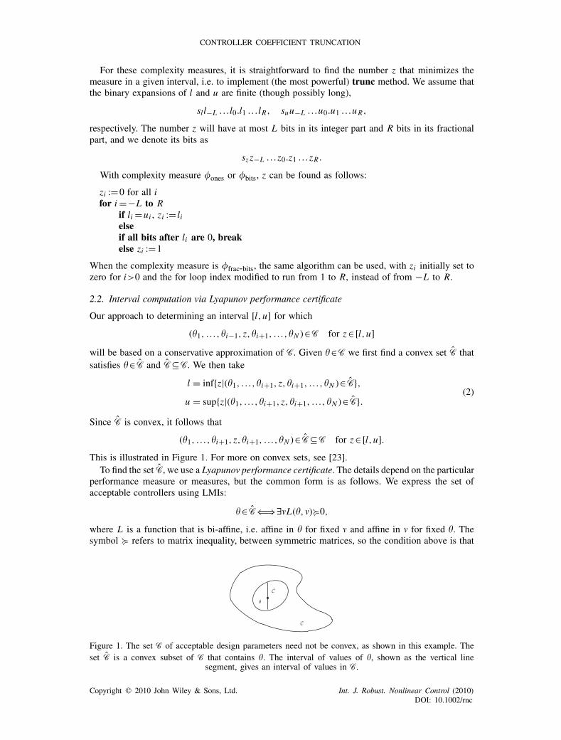
This is illustrated in Figure 1. For more on convex sets, see [23].To find the set C, we use a Lyapunov performance certificate. The details depend on the particular

performance measure or measures, but the common form is as follows. We express the set ofacceptable controllers using LMIs:

!" C()*%L(!,%)#0,

where L is a function that is bi-affine, i.e. affine in ! for fixed % and affine in % for fixed !. Thesymbol # refers to matrix inequality, between symmetric matrices, so the condition above is that

Figure 1. The set C of acceptable design parameters need not be convex, as shown in this example. Theset C is a convex subset of C that contains !. The interval of values of !, shown as the vertical line

segment, gives an interval of values in C.



L(!,%) is positive semidefinite. The variable % represents the coefficients in the Lyapunov functionused to certify the performance. For more on representing control system specifications via LMIs,see, e.g. [24–26].

For a given !"C, we compute a value of % such that L(!,%)#0. We then fix %, and take

C={!|L(!,%)#0}. (3)

This set depends on the particular choice of %; but in all cases, it is convex, indeed, it is described byan LMI in !. For a given !"C, % can be typically chosen to maximize the minimum eigenvalue ofL(!,%) or to maximize the (log of the) determinant of L(!,%). Both of these problems are convex:maximizing the minimum eigenvalue can be reduced to solve a semidefinite program (SDP) [27]and maximizing the determinant can be reduced to solving a MAXDET problem [28].

To find l or u in (2), we need to minimize or maximize a scalar variable over an LMI. This canbe reduced to an eigenvalue computation [23, Exer. 4.38], and can be carried out efficiently. SinceL(!,%) is bi-affine in ! and %, it can be expressed as

L(!,%)= L0+N!i=1

!i Li ,

where we have obscured the fact that the matrices L0 and Li depend on %. When !=(!1, . . . ,!i&1, z,!i+1, . . . ,!N ), we have

L(!,%)= L(!,%)+(z&!i )Li .

Assuming that L(!,%)+0, the range [l,u] of !i consists of the values of z for which L(!,%)#0. Itcan be shown that

l=!i &min{1/&i |&i>0}, u=!i &max{1/&i |&i<0}, (4)

where &i are the eigenvalues of L(!,%)&1/2Li L(!,%)&1/2.In the examples we will consider, the LMIs that arise have an even more specific form,

L(!,%)=$I ZT

Z I

%

#0,

where

Z = Z0+N!i=1

!iviwTi .

Here Z0 is a matrix, and vi and wi are vectors, with dimensions and data that depend on theparticular problem. In the general notation used above, this corresponds to

L0=$

I ZT0

Z0 I

%

, Li =$

0 wivTi

viwTi 0

%

, i =1, . . . ,N.

We can then express C as

C={!|,Z,!1},

where , ·, denotes the spectral norm (maximum singular value).We now give the details of how to find the range of the coefficient !i in the convex set C, i.e.

how to compute l and u in (2).Note that the rank of Li is exactly 2. Assuming that L(!,%)+0 and vi and wi are both nonzero,

the matrix L(!,%)&1/2Li L(!,%)&1/2 has one positive eigenvalue &max, (2n+m&2) zero eigenvalues,and one negative eigenvalue &min. We now proceed to find more explicit expressions for &min and



&max. Let Z =U"V T be the full singular value decomposition of Z where U and V are orthogonalmatrices and " has the same dimensions as Z . If m=n, " is diagonal. If m"n, we have

"=$diag('1, . . . ,'n)

0

%.

Otherwise, we have

"= [diag('1, . . . ,'m) 0].

Let

x =UT vi , y=V Twi , E=$I "T

" I

%, F=

$0 yxT

xyT 0

%.

Using a block Cholesky factorization, we can write E=CCT , where

C=$I 0

" (I &""T )1/2

%.

Note that

C&1=$

I 0

&A" A

%,

where A= (I &""T )&1/2.It is easy to show that &min and &max are, respectively, the minimum and maximum eigenvalues

of C&1FC&T. Since

F=$0 y

x 0

%$yT 0

0 xT

%,

and since non-zero eigenvalues of MN and NM are identical for any two matrices M "Rn-m andN "Rm-n, &min and &max are the eigenvalues of

$yT 0

0 xT

%

C&TC&1

$0 y

x 0

%

.

These can be found analytically as

&min = &(&&3(2+)yT y+)*, (5)

&max = &(+&3(2+)yT y+)*. (6)

The terms (, ), and * can be computed more easily as

( = xT A2"y=min{m,n}!

i=1

xi yi'i1&'2i

, (7)

) = xT A2x=m!i=1

x2i1&'2i

, (8)

* = yT"T A2"y=n!j=1

y2j'2j

1&'2j. (9)



In summary, to find l and u, we start by computing the SVD of the Z and setting x =UT vi ,y=V Twi . We then proceed to compute the three terms in (7)–(9) and compute &min and &maxfrom (5) and (6). Finally, l and u are found from (4):

l=!i &1/&max, u=!i &1/&min. (10)

3. STATE FEEDBACK CONTROLLER WITH LQR COST

We will demonstrate how to apply the algorithm to a specific problem class where the plant isgiven by

x(t+1)= Ax(t)+Bu(t), x(0)= x0, (11)

and is controlled by a state feedback gain controller given by

u(t)=Kx(t), (12)

where A"Rn-n , B"Rn-m , C"Rk-n , K "Rm-n is the feedback gain matrix, x(t)"Rn is the stateof the system, and u(t)"Rm is the input to the system. The design variables are the entries of thematrix K .

3.1. Admissible controllers

Given Q"Rn-n as positive semidefinite and R"Rm-m as positive definite, the performancemeasure is given by the LQR cost

J (K )=E' %!t=0

x(t)T Qx(t)+u(t)T Ru(t)(

=E' %!t=0

x(t)T (Q+KT RK)x(t)(, (13)

where the expectation is taken over x0.N(0,"). If A+BK is unstable J (K ) is infinite. Otherwise,let P be the (unique) solution to the Lyapunov equation

(A+BK)T P(A+BK)&P+Q+KTRK=0. (14)

The cost in (13) can be expressed as J (K )=Tr("P). This holds because

J (K )=E' %!t=0

x(t)T Px(t)&x(t)T (A+BK)T P(A+BK)x(t)(

=E' %!t=0

x(t)T Px(t)&x(t+1)T Px(t+1)(

=E[xT0 Px0]

=Tr(E[x0xT0 ]P)

=Tr("P).

The nominal design K nom is chosen to be the optimal state feedback controller, i.e. the one thatminimizes the LQR cost J . It can be found as follows:

K nom=&(R+BT PnomB)&1BT PnomA,

where Pnom is the solution of the discrete-time algebraic Riccati equation

Pnom=Q+AT PnomA&AT PnomA(R+BT PnomB)&1BT PnomA.



When K =K nom, Pnom is also the solution of the Lyapunov equation (14). The LQR cost associatedwith the optimal controller is J nom =Tr("Pnom).

We define the set of admissible controller design as

C={K |J (K )!(1+")J nom},

where " is a given positive number. This means that a controller design is admissible if and onlyif it is "-suboptimal.

We choose the Lyapunov performance certificate L to be

L(K , P)=

)

**+

P&(A+BK )T P(A+BK )&Q&KT RK 0 0

0 (1+")J nom&Tr("P) 0

0 0 P

,

--. .

Here K and P correspond, respectively, to ! and % introduced in Section 2.2. The condition thatL(K , P)#0 is equivalent to

(A+BK )T P(A+BK )&P+Q+KT RK $ 0,

Tr("P)! (1+")J nom, (15)

P # 0. (16)

As (15) and (16) do not depend on K , and for a particular choice P , (3) becomes

C={K |(A+BK )T P(A+BK )&P+Q+KT RK$0}. (17)

Given K "C, any matrix P that satisfies L(K , P)#0 is a valid choice. We take P to be the solutionof the following optimization problem

maximize &min(L(K , P))

subject to L(K , P)#0.

Here &min(L(K , P)) is the minimum eigenvalue of L(K , P) and P is the variable we are optimizingover. Recall that K is fixed.

We will now show that C#C. Let K " C. Consider the Lyapunov function V :Rn $R definedas V (z)= zT Pz. For any T>0,

V (x(T ))&V (x(0))=T!t=0

V (x(t+1))&V (x(t))

=T!t=0

x(t+1)T Px(t+1)&x(t)T Px(t)

=T!t=0

x(t)T ((A+BK )T P(A+BK )&P)x(t)

! &T!t=0

x(t)(Q+KT RK )x(t).

Therefore,

T!t=0

x(t)(Q+KT RK )x(t)!V (x(0))&V (x(T ))!V (x(0)),

where the last inequality follows because V (x(T ))"0 from (16). Letting T tend to infinity andtaking expectation over x0, we obtain J (K )!Tr("P). It follows from (15) that

J (K )!(1+")J nom.



3.2. Coefficient range calculation

Let (l,u) be the range of coefficient Ki j . Given (17), problem (2) becomes

l =min{Ki j |(A+BK )T P(A+BK )&P+Q+KT RK$0},

u =max{Ki j |(A+BK )T P(A+BK )&P+Q+KT RK$0}.

The inequality in (17) is equivalent to/////

$P1/2(A+BK )

R1/2K

%

(P&Q)&1/2

/////!1. (18)

The method outlined in Section 2.2 can be used to compute l and u by taking

Z =$P1/2(A+BK )

R1/2K

%

(P&Q)&1/2,

v =$P1/2B

R1/2

%

ei , w= (P&Q)&1/2e j ,

where ei and e j are, respectively, the i th unit vector in Rm and j th unit vector in Rn and K " Cis the current admissible controller design.

3.3. Numerical instance

Our example has dimensions n=10 and m=5. We generated the plant randomly, as A= I+0.1X/

/n, where Xi j are independent and identically distributed (IID) N(0,1). We generated the

matrix B"R10-5 with Bi j IID N(0,1). We take "= I , Q= I , and R= I .The complexity measures #i (z) are chosen to be #frac-bits. The fractional part of each entry of

K nom is expressed with 40 bits, requiring a total of 2000 bits to express K nom, i.e. !(!nom)=2000bits. We take "=15%, i.e. admissible feedback controllers are those that are up to 15% suboptimal.

The progress of the complexity !(!) during a sample run of the algorithm is shown in Figure 2.In this sample run the algorithm converges to a complexity of 85 bits in one pass over the variables.During the run of the algorithm the cost J is approximately constant and equal to its maximumallowed value of 1.15J nom.

The best design after 10 random runs of the algorithm achieves a complexity of !(!)=81 bits,with a cost of J (!)=1.1494J (!nom). The best design found after 100 random runs of the algorithmachieves a complexity of !(!)=75 bits and J (!)=1.1495J (!nom).

This best design gives very aggressive coefficient truncation with only 1.5 bits per coefficient.This is illustrated in Figure 3, which shows the distribution of the (50) coefficients of the nominaldesign and the coefficients of the best design. We observe that most of the coefficients in thebest design are 0 while the remaining ones have a complexity of at most 3 bits (for example for!i =0.125).

3.3.1. Multiple random instances. We report above the results for one random instance of theproblem. We now generate 100 random instances of A and B with other problem data the same(i.e. n=10,m=5, "= I , Q= I , R= I , "=15%). For each instance, we compute K nom and expressthe fractional part of each of its entries with 40 bits (i.e. #(!nom)=2000 bits).

For each instance, we record the best design after 10 random runs of the algorithm. Thecomplexities of the best designs range between 74 and 127 bits, with a mean of 98.29 bits anda standard deviation of 11.2 bits. The performance degradations of these designs ranged between14.88 and 14.99%. For these designs, the algorithm converged in an average of 1.1250 passes overthe variables. Thus the results reported in single instance case above are quite typical.



0 10 20 30 40 50 60 70 80 90 1000

200

400

600

800

1000

1200

1400

1600

1800

2000

Figure 2. Total number of bits required to express ! versus iteration number.

0 0.25 0.5 0.75 10

2

4

6

8

10

0 0.25 0.5 0.75 10

5

10

15

20

25

Figure 3. Top: Histogram of coefficients in the nominal design. Bottom: Histogram of coefficients in thebest design out of 10 random runs.

We can compare the results obtained with a simpler approach, in which we truncate the binaryexpansions of the coefficients to precision 2&q (i.e. with q bits in their fractional parts), choosingq as small as possible while still maintaining !"C. For the 100 random instances that weregenerated, q varied between 3 and 5 bits per coefficient with a mean of 4.57 bits. In contrast, ouralgorithm gave aggressively truncated controllers, with coefficient complexity between 1.48 and2.54 bits per coefficient, with a mean of 1.96 bits per coefficient.



4. DYNAMIC CONTROLLER WITH DECAY RATE SPECIFICATION

We demonstrate how to apply the algorithm to the problem class where the plant is given by

xp(t+1)= Apxp(t)+Bpu(t), y(t)=Cpxp(t), (19)

and is controlled by a dynamic controller given by

xc(t+1)= Acxc(t)+Bcy(t), u(t)=Ccxc(t), (20)

where xp(t)"Rnp , u(t)"Rmc , y(t)"Rmp , Ap "Rnp-np , Bp "Rnp-mc , Cp "Rmp-np , xc(t)"Rnc ,Ac "Rnc-nc , Bc"Rnc-mp , and Cc"Rmc-nc .The closed-loop system is given by x(t+1)= Ax(t) where

x(t)=$xp(t)

xc(t)

%, A=

$Ap BpCc

BcCp Ac

%. (21)

The design variables are the entries of the controller matrices Ac, Bc, and Cc.


A controller (Ac, Bc,Cc) is admissible if the decay rate of the closed-loop system is less than agiven rate (, where 0!(!1. The decay rate is given by +(A), where A is the matrix specified in(21).

The performance measure is chosen to be the decay rate of the closed-loop system, i.e.J (Ac, Bc,Cc)=+(A).We are given a nominal controller design (Anom

c , Bnomc ,Cnom

c ) such that

J (Anomc , Bnom

c ,Cnomc )=+.

We define the set of admissible controller designs as

C={(Ac, Bc,Cc)|J (Ac, Bc,Cc)!(},

where (= (1+")+, and " is a given positive number.We choose the Lyapunov performance certificate L to be

L(Ac, Bc,Cc, P)=$

(2P&AT PA 0

0 P

%

,

where A is the matrix defined in (21). Here (Ac, Bc,Cc) and P correspond, respectively, to ! and% introduced in Section 2.2. The condition that L(Ac, Bc,Cc, P)#0 is equivalent to

AT PA $ (2P,

P # 0.(22)

As (22) does not depend on (Ac, Bc,Cc), for a fixed choice of P , (3) becomes

C={(Ac, Bc,Cc)|AT PA!(2P}. (23)

Any matrix P that satisfies L(Ac, Bc,Cc, P)#0 for (Ac, Bc,Cc)"C is a valid choice. We take Pto be the solution of the following optimization problem

maximize &min(L(Ac, Bc,Cc, P))

subject to L(Ac, Bc,Cc, P)#0

Tr(P)=1.



Here &min(L(Ac, Bc,Cc, P)) is the minimum eigenvalue of L(Ac, Bc,Cc, P), and P is the variablewe are maximizing over. Recall that Ac, Bc, and Cc are fixed. The constraint Tr(P)=1 is addedbecause L(Ac, Bc,Cc, P) is homogeneous in P .

We will now show that C#C. Let (Ac, Bc,Cc)" C. Consider the Lyapunov function V :Rnp+nc $R defined as V (z)= zT Pz. Since AT PA!(2P then for all t"0

x(t)T AT PAx(t)! (2x(t)T Px(t)

x(t+1)T Px(t+1)! (2x(t)T Px(t)

V (x(t+1))! (2V (x(t)).

This means that for all t"0, V (x(t))!(2t V (x(0)) and

&min(P),x(t),2!x(t)T Px(t)!(2t x(0)T Px(0)!(2t&max(P),x(0),2,

then ,x(t),!/,(P)(t,x(0),, where ,(P) is the condition number of P . The decay rate of the

system is then less than (, as required.


Let (l,u) be the range of coefficient (Ac)i j . Given (23), problem (2) becomes

l =min{(Ac)ij|AT PA!(2P},

u =max{(Ac)ij|AT PA!(2P}.

The inequality in (23) is equivalent to

,P1/2AP&1/2,!(. (24)


Z = (1/()P1/2AP&1/2, v= (1/()P1/2

$0

ei

%, w= P&1/2

$0

e j

%,

where ei and e j are, respectively, the i th and j th unit vectors in Rnc and A is the closed-loopmatrix associated with (Ac, Bc,Cc)" C.

The same method can be used to find the ranges of coefficients in Bc and Cc and the sameformulas can be used but with slightly modified definitions for v and w. To find the range ofcoefficient (Bc)i j , use the same definitions for Z and v but let

w= P&1/2

$CT

p ej

0

%

,

where e j is the j th unit vector in Rmc . To find the range of coefficient (Cc)ij, use the samedefinitions for Z and w but let

v= (1/()P1/2

$Bpei

0

%

,

where ei is the i th unit vector in Rmc .


We test the proposed method in the case where the plant is given by

xp(t+1)= Apxp(t)+Bpu(t)+w(t), y(t)=Cpxp(t)+v(t), (25)



where w(t).N(0, I ) is the input noise and v(t).N(0, I ) is the measurement noise. The plantis controlled by an LQG controller with Q= I , R= I . The matrices describing the controller are

Ac= Ap+BpK &LCp, Bc= L, Cc=K , (26)

where

K =&(BTp P1Bp+R)&1BT

p P1Ap, L= Ap P2CTp (Cp P2CT

p +V )&1. (27)

P1 and P2 are the unique positive semidefinite solutions to the discrete-time algebraic Riccatiequations

P1 = ATp P1Ap+Q&AT

p P1Bp(R+BTp P1Bp)&1BT

p P1Ap,

P2 = Ap P2ATp +W&Ap P2CT

p (CpP2CTp +V )&1CpP2AT

p .

Our example has dimensions np =5, mc=2, and mp =2. The plant matrix Ap is randomlygenerated using the same method used to generate A in Section 3.3. The entries of Bp and Cp areIID N(0,1). The matrices Anom

c , Bnomc , and Cnom

c are then computed using the formulas presentedabove.

The complexity measures #i (z) are chosen to be #frac-bits. The fractional part of each entry ofAnomc , Bnom

c , and Cnomc is expressed with 40 bits, requiring a total of 1800 bits, i.e. !(!nom)=1800

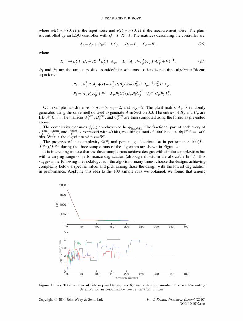
bits. We run the algorithm with "=5%.The progress of the complexity !(!) and percentage deterioration in performance 100(J&

J nom)/J nom during the three sample runs of the algorithm are shown in Figure 4.It is interesting to note that the three sample runs achieve designs with similar complexities but

with a varying range of performance degradation (although all within the allowable limit). Thissuggests the following methodology: run the algorithm many times, choose the designs achievingcomplexity below a specific value, and pick among those the design with the lowest degradationin performance. Applying this idea to the 100 sample runs we obtained, we found that among

0 50 100 150 200 250 300 350 4000

500

1000

1500

2000

0 50 100 150 200 250 300 350 4000

1

2

3

4

5

Figure 4. Top: Total number of bits required to express !, versus iteration number. Bottom: Percentagedeterioration in performance versus iteration number.



0 10 20 30 40 50 60 70 80 90 100160

165

170

175

180

185

190

195

200

205

Figure 5. Best design complexity versus number of sample runs of the algorithm.

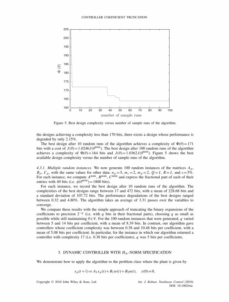
the designs achieving a complexity less than 170 bits, there exists a design whose performance isdegraded by only 2.15%.

The best design after 10 random runs of the algorithm achieves a complexity of !(!)=171bits with a cost of J (!)=1.0246J (!nom). The best design after 100 random runs of the algorithmachieves a complexity of !(!)=164 bits and J (!)=1.0362J (!nom). Figure 5 shows the bestavailable design complexity versus the number of sample runs of the algorithm.

4.3.1. Multiple random instances. We now generate 100 random instances of the matrices Ap ,Bp , Cp , with the same values for other data: np =5, mc=2, mp =2, Q= I , R= I , and "=5%.For each instance, we compute Anom, Bnom, Cnom and express the fractional part of each of theirentries with 40 bits (i.e. #(!nom)=1800 bits).

For each instance, we record the best design after 10 random runs of the algorithm. Thecomplexities of the best designs range between 17 and 472 bits, with a mean of 228.68 bits anda standard deviation of 107.72 bits. The performance degradations of the best designs rangedbetween 0.32 and 4.80%. The algorithm takes an average of 3.31 passes over the variables toconverge.

We compare these results with the simple approach of truncating the binary expansions of thecoefficients to precision 2&q (i.e. with q bits in their fractional parts), choosing q as small aspossible while still maintaining !"C. For the 100 random instances that were generated, q variedbetween 5 and 14 bits per coefficient, with a mean of 8.39 bits. In contrast, our algorithm gavecontrollers whose coefficient complexity was between 0.38 and 10.48 bits per coefficient, with amean of 5.08 bits per coefficient. In particular, for the instance in which our algorithm returned acontroller with complexity 17 (i.e. 0.38 bits per coefficients), q was 5 bits per coefficients.

5. DYNAMIC CONTROLLER WITH H%-NORM SPECIFICATION

We demonstrate how to apply the algorithm to the problem class where the plant is given by

xp(t+1)= A1xp(t)+B1w(t)+B2u(t), x(0)=0,



z(t)=C1xp(t)+D11w(t)+D12u(t),

y(t)=C2xp(t)+D21w(t),

and is controlled by a dynamic controller given by

xc(t+1)= Acxc(t)+Bcy(t), u(t)=Ccxc(t)+Dcy(t), xc(0)=0.

where xp(t)"Rnp , u(t)"Rmc , w(t)"Rk, y(t)"Rmp , and xc(t)"Rnc .The closed-loop system is given by

x(t+1)= Ax(t)+Bw(t), z(t)=Cx(t)+Dw(t),

where

x(t)=$xp(t)

xc(t)

%

, A=$A1+B2DcC2 B2Cc

BcC2 Ac

%

, B=$B1+B2DcD21

BcD21

%

, (28)

C = [C1+D12DcC2 D12Cc], D=D11+D12DcD21. (29)

The design variables are the entries of the controller matrices Ac, Bc, Cc, and Dc.


Let G(s) be the transfer function of the closed-loop system. The H% norm of G(s) is its largestinput/output RMS gain, i.e.

,G,% = supu '=0

,z,2,w,2

,

where z(t) is the output of the closed-loop system for a given input w(t), and where

,x,2=0

limT$%

1T

T!t=0

,x(t),211/2

,

for any signal x(t), t"0.The performance measure J (Ac, Bc,Cc,Dc) is chosen to be the H% norm of the transfer function

of the closed-loop system.We are given a nominal controller design (Anom

c , Bnomc ,Cnom

c ,Dnomc ) such that

J (Anomc , Bnom

c ,Cnomc ,Dnom

c )=*nom.

A controller (Ac, Bc,Cc,Dc) is admissible if the H% norm of the transfer function of the closed-loop transfer function is less than a given value *>0, where *= (1+")*nom for given a positivenumber ". In other words, the set of admissible controller designs is

C={(Ac, Bc,Cc,Dc)|J (Ac, Bc,Cc,Dc)!*}.

Note that (Anomc , Bnom

c ,Cnomc ,Dnom

c )" C.We take the Lyapunov performance certificate to be

L(Ac, Bc,Cc,Dc, P)=

)

**+

P&ATPA&CTC &AT PB&CT D 0

&BT PA&DTC *2 I &BT PB&DT D 0

0 0 P

,

--. ,



where A, B, C , D are the matrices introduced in (28) and (29). Here (Ac, Bc,Cc,Dc) and P corre-spond, respectively, to ! and % introduced in Section 2.2. The condition that L(Ac, Bc,Cc, P)#0is equivalent to

$AT PA&P+CTC AT PB+CT D

BT PA+DTC BT PB+DT D&*2 I

%

$ 0,

P # 0. (30)

As (30) does not depend on (Ac, Bc,Cc,Dc), for a fixed choice of P , (3) becomes

C=2

(Ac, Bc,Cc,Dc)

33333

$AT PA&P+CTC AT PB+CT D

BTPA+DTC BT PB+DT D&*2 I

%

$0

4

. (31)

Any matrix P that satisfies L(Ac, Bc,Cc,Dc, P)#0 for (Ac, Bc,Cc,Dc)"C is a valid choice.We take P to be the solution of the following optimization problem

maximize &min(L(Ac, Bc,Cc,Dc, P))

subject to L(Ac, Bc,Cc,Dc, P)#0.

Here &min(L(Ac, Bc,Cc,Dc, P)) is the minimum eigenvalue of L(Ac, Bc,Cc, P), and P is thevariable we are optimizing over. Recall that Ac, Bc, Cc, and Dc are fixed.

We will now show that C#C. Let (Ac, Bc,Cc,Dc)" C. Consider the Lyapunov function V :Rnp+nc $R defined as V (z)= zT Pz. For all x , w,

$x

w

%T $AT PA&P+CTC AT PB+CT D

BT PA+DTC BT PB+DT D&*2 I

%$x

w

%!0,

or equivalently

(Ax+Bw)T P(Ax+Bw)&xT Px!*2wTw&(Cx+Dw)T (Cx+Dw).

For all t ,

V (x(t+1))&V (x(t))!*2w(t)Tw(t)&z(t)T z(t).

We know that V (x(0))=0. Since (30) implies that V (x(T ))"0 and since

V (x(T ))&V (x(0)=T!t=0

V (x(t+1))&V (x(t)),

we deduce that

0!T!t=0

V (x(t+1))&V (x(t))!T!t=0

*2w(t)Tw(t)&z(t)T z(t).

Therefore

T!t=0

z(t)T z(t)!*2T!t=0

w(t)Tw(t) (32)

holds for all T>0. Dividing by T and letting T tend to infinity on both sides of (32), we obtain,z,2!*2,w,2 which implies that the H% norm of the transfer function of the closed-loop systemis less than or equal to * as desired.




Let (l,u) be the range of coefficient (Ac)i j . Given the equation in (31), problem (2) becomes

l =min{(Ac)i j |AT PA&P+CTC+(AT PB+CT D)Q(BT PA+DTC)$0},

u =max{(Ac)i j |AT PA&P+CTC+(AT PB+CT D)Q(BT PA+DTC)$0},

where Q=*2 I &BT PB&DT D. The inequality in (31) is equivalent to/////

$P1/2AP&1/2 *&1P1/2B

CP&1/2 *&1D

%/////!1. (33)


Z =$P1/2AP&1/2 *&1P1/2B

CP&1/2 *&1D

%

, v=$P1/2

0

%$0

ei

%

, w=$P&1/2

0

%$0

e j

%

, (34)

where ei and e j are the i th and j th unit vectors in Rnc and (A, B,C,D) is the closed-loop matrixassociated with (Ac, Bc,Cc,Dc)" C.

The same method can be used to find the ranges of coefficients in Bc, Cc, and Dc. The sameformulas can be used but with slightly modified definitions for v and w. To find the range ofcoefficient (Bc)ij, use the same definitions for Z and v in (34) but let

w=

)

**+P&1/2

$CT2

0

%

*&1DT21

,

--.e j , (35)

where e j is the j th unit vector in Rmp . To find the range of coefficient (Cc)i j , use the samedefinitions for Z and w in (34) but let

v=

)

**+P1/2

$B2

0

%

D12

,

--.ei , (36)

where ei is the i th unit vector in Rmc . To find the range of coefficient (Dc)i j , use the definitionfor Z given in (34), the definition of v given in (36) and the definition of w given in (34).


Our example has dimensions np =5, nc=4, mp =2, mc=2, and k=3. We generate matrix Apusing the method used to generate A in Section 3.3. The entries of the matrices B1, B2, C1, C2,D11, D12, D21 are IID N(0,1).The nominal controller (Anom

c , Bnomc ,Cnom

c ,Dnomc ) is chosen to be the central H% controller, i.e.

the one that minimizes the H% norm of the transfer function of the closed-loop system (see, e.g.[29, 30]).


c , Cnomc , Dnom

c is expressed with 40 bits, requiring a total of 1440 bits, i.e. !(!norm)=1440 bits. We run the basic algorithm with "=15%, which means that we allow the H% norm ofthe controller to be up to 15% suboptimal.

The progress of the complexity !(!) and percentage deterioration in performance 100(J&J nom)/J nom during the three sample runs of the algorithm are shown in Figure 6.It is interesting to note that the three sample runs achieve designs with similar complexities but

with a varying range of performance degradation (although all within the allowable limit). This



0 20 40 60 80 100 120 140 160 180 200200

400

600

800

1000

1200

1400

1600

0 20 40 60 80 100 120 140 160 180 200

0

0.2

0.4

0.6

0.8

1

1.2

Figure 6. Top: Total number of bits required to express ! versus iteration number. Bottom: Percentagedeterioration in performance versus iteration number.

suggests the following methodology: run the algorithm many times, choose the designs achievingcomplexity below a specific value, and pick among those the design with the lowest degradationin performance. Applying this idea to the 100 sample runs we obtained, we found that amongthe designs achieving a complexity less than 260 bits, there exists a design whose performance isdegraded by only 1.15%.

The best design after 10 random runs of the algorithm achieves a complexity of !(!)=270bits with a cost of J (!)=1.002J (!nom). The best design after 100 random runs of the algorithmachieves a complexity of !(!)=247 bits and J (!)=1.030J (!nom).

5.3.1. Multiple random instances. We now generate 100 random instances of matrices Ap , B1, B2,C1, C2, D11, D12, D21, with other data remaining the same: np =5, nc=4,mp =2, mc=2, k=3,and "=15%. For each instance, we compute Anom, Bnom, Cnom, Dnom and express the fractionalpart of each of their entries with 40 bits.

For each instance, we record the best design after 10 random runs of the algorithm. Thecomplexities of the best designs range between 170 and 403 bits, with a mean of 274.21 bits and astandard deviation of 59.54 bits. The performance degradations of the best designs ranged between0.04 and 14.52%. The algorithm takes an average of 1.5 passes over the variables to converge.

We compare these results with the simple approach of truncating the binary expansions of thecoefficients to precision 2&q (i.e. with q bits in their fractional parts), choosing q as small aspossible while still maintaining !"C. For the 100 random instances that were generated, q variedbetween 8 and 40 bits per coefficient with a mean of 18.72 bits. In contrast, our algorithm gavecontrollers whose coefficient complexity was between 4.77 and 11.19 bits per coefficient, with amean of 7.63 bits per coefficient.

6. DYNAMIC CONTROLLER WITH SATURATION

We have been dealing with specifications on linear closed-loop systems until now. The methodologythat we covered can be easily extended to the case where we are given specifications on closed-loop



systems with nonlinear dynamics. We illustrate this idea through the following example where theplant is given by

xp(t+1)=Apxp(t)+Bpu(t), y(t)=Cpxp(t),

and is controlled by a dynamic controller given by the nonlinear dynamical system

xc(t+1)= sat(Acxc(t)+Bcy(t)),

u(t)= sat(Ccxc(t)),

where xp(t)"Rnp , u(t)"Rmc , y(t)"Rmp , Ap "Rnp-np , Bp "Rnp-mc , Cp "Rmp-np , xc(t)"Rnc ,Ac "Rnc-nc , Bc"Rnc-mp , and Cc"Rmc-nc , and sat :R$R is defined as

sat(z)=

567

68

z if |z|!1

&1 if z<&1

1 if z>1.

The closed-loop system is a nonlinear dynamical system of the form

x(t+1) = Ax(t)+Bp(t),

q(t) = Cx(t),

pi = sat(qi ), i =1, . . . ,mc+nc,

(37)

where

x(t) =$xp(t)

xc(t)

%, A=

$Ap 0

0 0

%,

B =$Bp 0

0 I

%

, C=$

0 Cc

BcCp Ac

%

.

(38)


We define the decay rate of the closed-loop system to be the infinimum of ( for which everytrajectory of the closed-loop system satisfies

,x(t),!M(t,x(0),,

for all t and for some M>0. Here M is a constant that depends on the trajectory.The performance measure J is chosen to be the decay rate of the closed-loop system. Unlike

the other cases we presented, it is very difficult to compute the decay rate J of the closed-loopsystem described in (37). However, as we shall subsequently see, an upper bound on the decayrate can be found using a Lyapunov method.

We are given nominal design (Anomc , Bnom

c ,Cnomc ) with a decay rate less than +.

A controller (Ac, Bc,Cc) is admissible if the decay rate of the closed-loop system is less than agiven rate (, where (= (1+")+ and " is a given positive number. The set of admissible controllerdesigns is then

C={(Ac, Bc,Cc)|J (Ac, Bc,Cc)!(}.

We choose the Lyapunov performance certificate to be

L(Ac, Bc,Cc, P,-1, . . . ,-mc+nc )=

)

*****+

(2P&AT PA &AT PB&(1/2)CT D 0 0

&BT PA&(1/2)DC D&BT PB 0 0

0 0 P& I 0

0 0 0 D

,

-----.



where D=diag(-1, . . . ,-mc+nc ) and A, B, and C are the matrices introduced in (38). Here(Ac, Bc,Cc) correspond to ! and (P,-1, . . . ,-mc+nc ) correspond to % introduced in Section 2.2. Thecondition that L(Ac, Bc,Cc, P,-1, . . . ,-mc+nc )#0 is equivalent to

$AT PA&(2P AT PB+(1/2)CT D

BT PA+(1/2)DC BT PB&D

%

$ 0,

P # I, (39)

D # 0. (40)

Since (39) and (40) do not depend on (Ac, Bc,Cc) for a fixed choice of P and D, (3) becomes

C=2

(Ac, Bc,Cc)|$

AT PA&(2P AT PB+(1/2)CT D

BT PA+(1/2)DC BT PB&D

%

$0

4

. (41)

Any matrix P and scalars -1, . . . ,-mc+nc that satisfy L(Ac, Bc,Cc, P,D)#0 for given(Ac, Bc,Cc)"C are a valid choice. We take (P,D) to be the solution of the following optimizationproblem

maximize &min(L(Ac, Bc,Cc, P,D))

subject to L(Ac, Bc,Cc, P,D)#0,

D=diag(-1, . . . ,-mc+nc ).

Here &min(L(Ac, Bc,Cc, P)) is the minimum eigenvalue of L(Ac, Bc,Cc, P), and P , -1, . . . ,-mc+ncare the variables that we are optimizing over. Recall that Ac, Bc, and Cc are fixed here.

We will now show that C#C. Let (Ac, Bc,Cc)" C. Consider the Lyapunov functionV :Rnp+nc $R defined as V (z)= zT Pz. Note that pi and qi must satisfy (pi &qi )pi!0 fori =1, . . . ,mc+nc. Recalling that q=Cx , this means that, for all x and p,

$x

p

%T $0 &(1/2)CT D

&(1/2)DC D

%$x

p

%

!0. (42)

Since (Ac, Bc,Cc)" C, the following holds for all x , p,

$x

p

%T $AT PA&(2P AT PB+(1/2)CT D

BT PA+(1/2)DTC BTPB&D

%$x

p

%

!0. (43)

It follows from (42) and (43) that

$x

p

%T $AT PA&(2P AT PB

BTPA BT PB

%$x

p

%

!$x

p

%T $0 &(1/2)CT D

&(1/2)DC D

%$x

p

%

!0.

This inequality implies that

(Az+Bp)T P(Az+Bp)!(2zT Pz.

Therefore we have V (x(t+1))!(2V (x(t)) for all t"0. This implies that the decay rate of theclosed-loop system is less than (, as demonstrated in Section 3.1.




The inequality in (41) is an LMI in P and D, but in the given form it is a convex matrix quadraticinequality in (A, B,C). It can easily be shown that it is actually equivalent to the LMI in (A, B,C):

)

**+

(2P &(1/2)CT D AT

&(1/2)DC D BT

A B P&1

,

--.#0. (44)

Since (A, B,C) are linear in (Ac, Bc,Cc), (44) is also an LMI in (Ac, Bc,Cc). The range ofcoefficient of (Ac)i j can, therefore, be found from (4) by the eigenvalue computation methodoutlined in Section 2.2 with L(!,% given by (44) and

Li =

)

**+

0 &(1/2)vwT D 0

&(1/2)DwvT 0 0

0 0 0

,

--. ,

where

w=$0

ei

%, v=

$0

e j

%,

and ei and e j are, respectively, the i th and j th unit vectors in Rnc .The same method can be used to find the ranges of coefficients in Bc and Cc but with slightly

modified definitions for v and w. To find the range of coefficient (Bc)i j , take

w=$0

ei

%

, v=$CT

p e j

0

%

,

where ei is the i th unit vector in Rnc and e j is the j th unit vector in Rmp . To find the range ofcoefficient (Cc)ij, take

w=$ei

0

%

, v=$0

e j

%

,

where ei is the i th unit vector in Rmp and e j is the j th unit vector in Rnc .


We test the proposed method on the problem described in Section 4.3 where the plant is describedby (25) and where the nominal controller is described by (26) and (27). The decay rate + of theclosed-loop system is the minimum value of ( for which there exists matrices P and D that satisfy

L(Anomc , Bnom

c ,Cnomc , P,-, . . . ,-mc+nc )#0.

Our example has dimensions np =5, mc=2, and mp =2. The plant matrix Ap is randomlygenerated using the same method used to generate A in Section 3.3. The entries of Bp and Cp areIID N(0,1). The matrices Anom

c , Bnomc , and Cnom

c are then computed using the formulas presentedin Section 4.3.


c , and Cnomc is expressed with 40 bits, requiring a total of 1800 bits, i.e. !(!nom)=1800

bits. The decay rate of the nominal system is found to be 0.9326. We run the algorithm with"=5%.

The best design after 10 random runs of the algorithm achieves a complexity of !(!)=35 bits,with a cost of J (!)=0.9770J (!nom). The best design found after 100 random runs of the algorithm



achieves a complexity of !(!)=18 bits and J (!)=0.9288J (!nom) (which is smaller than the valuefor our nominal controller).

6.3.1. Multiple random instances. We generate 100 random instances of matrices Ap , Bp , Cp ,with other data remaining the same: np =5, mc=2, mp =2, Q= I , R= I , and "=5%. For eachinstance, we compute Anom, Bnom, Cnom and express the fractional part of each of their entrieswith 40 bits (i.e. #(!nom)=1800 bits).

For each instance, we record the best design after 10 random runs of the algorithm. Thecomplexities of the best designs range between 10 and 52 bits, with a mean of 22.85 bits and astandard deviation of 9.6 bits. Moreover, the performance degradations of the best designs rangedbetween &9.21 and 0.61% and the algorithm takes an average of six passes over the variables toconverge. (Here negative values mean that the objective value of our truncated controller is smallerthan that of the nominal controller).

We compare these results with the simple approach of truncating the binary expansions of thecoefficients to precision 2&q (i.e. with q bits in their fractional parts), choosing q as small aspossible while still maintaining !"C. For the 100 random instances that were generated, q variedbetween 3 and 8 bits per coefficient with a mean of 5.55 bits. In contrast, our algorithm gaveaggressively truncated controllers whose complexity was between 0.22 and 1.16 bits per coefficient,with a mean of 0.51 bits per coefficient.

ACKNOWLEDGEMENTS

This work was funded in part by Focus Center Research Program Center for Circuit and System Solutions(www.c2s2.org), under contract 2003-CT-888, by AFOSR grant AF F49620-01-1-0365, by NSF grantECS-0423905, by NSF grant 0529426, by DARPA/MIT grant 5710001848, by AFOSR grant FA9550-06-1-0514, DARPA/Lockheed contract N66001-06-C-2021, and by AFOSR/Vanderbilt grant FA9550-06-1-0312.

REFERENCES

1. Avenhaus E. On the design of digital filters with coefficients of limited word length. IEEE Transactions on Audioand Electroacoustics 1972; 20(3):206–212.

2. Brglez F. Digital filter design with short word-length coefficients. IEEE Transactions on Circuits and Systems1978; 25(12):1044–1050.

3. Gray A, Markel J. Quantization and bit allocation in speech processing. IEEE Transactions on Acoustics, Speech,and Signal Processing 1976; 24(6):459–473.

4. Rink R, Chong H. Performance of state regulator systems with floating point computation. IEEE Transactionson Automatic Control 1979; 14:411–412.

5. Lim Y, Yu Y. A successive reoptimization approach for the design of discrete coefficient perfect reconstructionlattice filter bank. IEEE International Symposium on Circuits and Systems, vol. 2, 2000; 69–72.

6. Samueli H. An improved search algorithm for the design of multiplierless FIR filters with powers-of-twocoefficients. IEEE Transactions on Circuits and Systems 1989; 36(7):1044–1047.

7. Lee J, Chen C, Lim Y. Design of discrete coefficient FIR digital filters with arbitrary amplitude and phase response.IEEE Transactions on Circuits and Systems—II: Analog and Digital Signal Processing 1993; 40(7):444–448.

8. Lim Y, Yu Y. A width-recursive depth-first tree search approach for the design of discrete coefficient perfectreconstruction lattice filter bank. IEEE Transactions on Circuits and Systems II 2003; 50:257–266.

9. Frossard P, Vandergheynst P, Figueras R, Kunt M. A posteriori quantization of progressive matching pursuitstreams. IEEE Transactions on Signal Processing 2004; 52(2):525–535.

10. Lim Y, Parker S. Discrete coefficient FIR digital filter design based upon an LMS criteria. IEEE Transactionson Acoustics, Speech, and Signal Processing 1983; 30(10):723–739.

11. Chen S, Wu J. The determination of optimal finite precision controller realizations using a global optimizationstrategy: a pole-sensitivity approach. In Digital Controller Implementation and Fragility: A Modern Perspective,Istepanian R, Whidborne J (eds), Chapter 6. Springer: New York, 2001; 87–104.

12. Benvenuto N, Marchesi M, Orlandi G, Piazza F, Uncini A. Finite wordlength digital filter design using anannealing algorithm. IEEE International Conference on Acoustics, Speech and Signal Processing (ICASSP), 1989;861–864.

13. Istepanian R, Whidborne J. Multi-objective design of finite word-length controller structures. Proceedings of theCongress on Evolutionary Computation, vol. 1, 1999; 61–68.



14. Gentili P, Piazza F, Uncini A. Efficient genetic algorithm design for power-of-two FIR filters. InternationalConference on Acoustics, Speech, and Signal Processing (ICASSP), 1995; 1268–1271.

15. Traferro S, Capparelli F, Piazza F, Uncini A. Efficient allocation of power-of-two terms in FIR digital filterdesign using tabu search. International Symposium on Circuits and Systems (ISCAS), 1999; III-411–414.

16. Li G, Covers M. Optimal finite precision implementation of a state-estimate feedback controller. IEEE Transactionson Circuits and Systems 1990; 37(12):1487–1498.

17. Wah B, Shang Y, Wu Z. Discrete Lagrangian methods for optimizing the design of multiplierless QMF banks.IEEE Transactions on Circuits and Systems II 1999; 46(9):1179–1191.

18. Kodek D. Design of optimal finite wordlength FIR digital filters using integer programming techniques. IEEETransactions on Acoustics, Speech, and Signal Processing 1980; 28(3):304–308.

19. Lim Y, Parker S. FIR filter design over a discrete powers-of-two coefficient space. IEEE Transactions onAcoustics, Speech, and Signal Processing 1983; 31(3):583–591.

20. Barua S, Kotteri K, Bell A, Carletta J. Optimal quantized lifting coefficients for the 9/7 wavelet. IEEE InternationalConference on Acoustics, Speech and Signal Processing (ICASSP), vol. 5, 2004; V-193–196.

21. Liu K, Skelton R, Grigoriadis K. Optimal controllers for finite wordlength implementation. IEEE Transactionson Automatic Control 1992; 37(9):1294–1304.

22. Molchanov A, Bauer P. Robust stability of digital feedback control systems with floating point arithmetic.Proceedings of the 34th Conference on Decision and Control 1995; 4251–4258.

23. Boyd S, Vandenberghe L. Convex Optimization. Cambridge University Press: Cambridge, 2004.24. Boyd S, El Ghaoui L, Feron E, Balakrishnan V. Linear Matrix Inequalities in Systems and Control Theory.

SIAM Books: Philadelphia, 1994.25. Boyd S, Barratt C. Linear Controller Design: Limits of Performance. Prentice-Hall: Englewood Cliffs, NJ, 1991.26. Dullerud G, Paganini F. A Course in Robust Control Theory: A Convex Approach. Springer: New York, 2000.27. Vandenberghe L, Boyd S. Semidefinite programming. SIAM Review 1996; 38(1):45–95.28. Vandenberghe L, Boyd S, Wu S. Determinant maximization with linear matrix inequality constraints. SIAM

Journal on Matrix Analysis and Applications 1998; 19(2):499–533.29. Gahinet P. Explicit controller formulas for LMI-based H% synthesis. American Control Conference, vol. 3, 1994;

2396–2400.30. Gahinet P, Apkarian P. A linear matrix inequality approach to H% control. International Journal on Robust and

Nonlinear Control 1994; 4:421–448.


jwuk rnc 1577 - stanford universityboyd/papers/pdf/contr_coef_trunc.pdf · the complexity of a...

Documents