United StatesDepartment ofAgriculture

Forest Service

Pacific SouthwestResearch Station

Research PaperPSW-RP-210

/kc> Ie 7- Zt/-9~q/-2!

A Diameter IncrementModel for Red Fir inCalifornia and SouthernOregon

K. Leroy Dolph

Dolph, K. Leroy. 1992. A diameter increment model for red fir in California andsouthern Oregon. Res. Paper PSW-RP-210. Albany, CA: Pacific Southwest ResearchStation, Forest Service, U.S. Department of Agriculture; 6 p.

Periodic (lO-year) diameter increment of individual red fir trees in Califomia andsouthern Oregon can be predicted from initial diameter and crown ratio of each tree, siteindex, percent slope, and aspect of the site. The model actually predicts the natural logarithmofthe change in squared diameter inside bark between thestart and the end ofa 1O-yeargrowthperiod. To estimate diameter increment, the predicted value is converted to a change indiameter outside bark. Data used to develop the model came from 1500 tree samples from56 young-growth stands in the study area. Coefficients forthe log-linear model were obtainedusing least-squares linear regression.

RetrievalTerms: increment (diameter), California red fir, Shasta red fir, California, Oregon

The Author:

K. LEROY DOLPH is a research forester assigned to the Station's Silviculture ofCalifornia Conifer Types Research Unit, 2400 Washington Avenue, Redding, CA 96001.

Publisher:

Pacific Southwest Research StationAlbany, California(Mailing address: P.O. Box 245, Berkeley, CA 94701-0245)Telephone: 510-559-6300)

March 1992

A Diameter Increment Modelfor Red Fir in California andSouthern Oregon

K. Leroy Dolph

Contents

In Brief ii

Introduction I

Methods 1

Stand and Tree Measurements 2

Site Factors 2

Analysis 2

Results and Discussion 3

The Independent Variables 3

Random Cluster Effect 4

Correcting for Log Bias 4

An Example 4

Confidence Limits 4

Estimating Future Diameters 5

Conclusions 5

References 6

In Brief ...

Dolph, K. Leroy. 1992. A diameter increment model for red firin California and southern Oregon. Res. PaperPSW-RP-21 O.Albany, CA: Pacific Southwest Research Station, Forest Ser­vice, U.S. Depmtment of Agriculture; 6 p.

Retrieval Terms: increment (diameter), California red fir, Shastared fir, California, Oregon

Red fir forests of California and southern Oregon are becom­ing more intensively managed for timber production and toenhance production and values of other resources. However,growth and yield information is presently limited in these high­elevation forests. Tltree geographic variants of the stand prog­nosis model (PROGNOSIS) (Stage 1973; Wykoff and others1982) have been developed for growth projection and yieldestimates of the major commercial tree species in California, butno growth functions for these variants exist for red fir.

A model was developed to predict periodic (IO-year) diam­eter increment of individual red fir trees in CalifOlnia and south­ern Oregon. The model actually predicts the natural logarithmof the change in squared diameter inside bark between the strutand the end of a IO-yem' growth period. To estimate diameter

ii

increment, the predicted value is converted to a change in diam~

eter outside bark.Individual tree characteristics and stand and site factor infor­

mation were recorded in 56 randomly selected young-growthred fir stands throughout the study area. Corresponding diam­eter growth for the past 10 years was measured from incrementcores of the sample trees. Least squares regression techniqueswere used to relate IO-year diameter £'Owth to the significanttree, stand, and site variables and to obtain estimates of themodel parameters.

InfOlmation needed to predict diameter increment (for afuture JO-yearperiod) ofindividual trees on a given site includesinitial diameter and crown ratio of each tree, site index, percentslope, and aspect of tl,e site. Additional stand variables neededfor the prediction, such as stand density (expressed as basal areaper acre) and the basal area made up of trees larger than thesubject tree, can be calculated directly from the diameters of theindividual stems.

The log-linear regression model accounted for 84.6 percentof the variabili ty in log of change in squared diameters observedon the study plots.

USDA Forest Service Res. Paper PSW-RP-21O. 1992.

Introduction

In recent years, red fir forests have become an increasinglyimportant natural resonrce in California. Not only is the de­mand for once "nonpreferred" wood now substantial, thesehigh-elevation forests occupy prime recreational and wildlifehabitat areas and much of the snowbelt that furnishes usablesurface water in the state. Growth and yield information there­fore becomes increasingly important for forest resource man­agement considerations in this forest type. Accurate estimatesof both current resource levels and the expected resourcechanges from implementing various management alternativesare needed for making wise management decisions.

The Prognosis Model for Stand Development (PROGNO­SIS), an individual tree growth and yield model, was devel­oped for use in the Inland Empire area of northern Idaho,eastern Washington, and western Montana (Stage 1973). New"variants" of PROGNOSIS result when that model is cali­brated for different geographic areas. Three variants ofPROG­NOSIS have been developed for growth projection and yieldestimates of the major commercial tree species in California,but no growth models exist for the red fir type.

This paper describes a log-linear regression model forpredicting future IO-year diameter increment for red fir inCalifornia and southern Oregon. This model is designed to beused within existing PROGNOSIS variants for silviculturaland management planning for the red fir type. Since Californiared fir (Abies magnifica A. Murr.) and its commonly recog­nized variety Shasta red fir (Abies magnifica var. shastensisLemm.) are considered to be almost identical in silvical char­acteristics (Hallin 1957), no attempt was made to distinguishbetween them during the sampling phase of the stndy. In thispaper they are referred to collectively as "red fir."

Methods

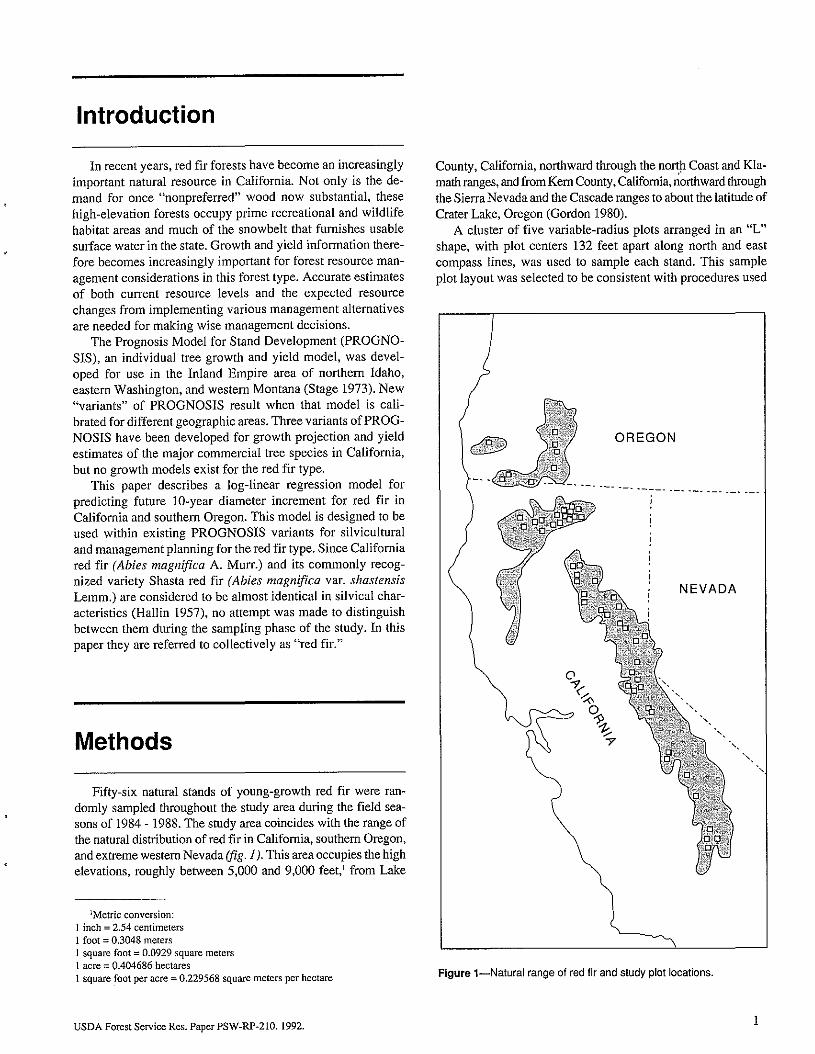
Fifty-six natural stands of young-growth red fir were ran­domly sampled throughout the study area during the field sea­sons of 1984 - 1988. The study area coincides with the range ofthe natural distribntion of red fir in California, southern Oregon,and extreme western Nevada (fig. 1). This area occupies the highelevations, roughly between 5,000 and 9,000 feet,' from Lake

lMetric conversion:I inch = 2.54 centimeters1 foot = 0.3048 metersI square foot = 0.0929 square meters1 acre = 0.404686 hectares1 square foot per acre = 0.229568 square meters per hectare

USDA Forest Service Res. Paper PSW-RP~21O. 1992.

County, California, northward through the north Coast and Kla­math ranges, and from Kern County, California, ';~rthward throughthe Sierra Nevada and the Cascade ranges to about the latitude ofCrater Lake, Oregon (Gordon 1980).

A clnster of five variable-radius plots arranged in an "L"shape, with plot centers 132 feet apart along north and eastcompass lines, was used to sample each stand. This sampleplot layout was selected to be consistent with procedures used

OREGON

---- --. --- --- -_. ---

NEVADA

Figure l-Natural range of red fir and study plot locations.

I

in the Pacific Southwest Region's Compartment Inventoryand Analysis (CIA) program. Each plot in the cluster wasindependently evaluated for study suitability by the followingcriteria:

• Homogeneous site-No more than one distinct soil type,slope percentage, or aspect was present on a D.2-acre circularplot around the plot center (radius 52.7 ft).

• Significant amount of red fir-At least 20 percent of thetrees 1.0 inch and greater in diameter at breast height (dbh)were red fir.

• Young-growth-No more than 25 percent of the plottrees were older than 120 years at breast height.

• Untreated stand-No silviculturaI treatment was evidentduring the 10 years before measurement.In stands where at least two of the five plots met these fourcriteria, all suitable plots were measured. If there were fewerthan two suitable plots, no measurements were taken in thatstand. The number of measured plots therefore ranged fromtwo to five in each of the clusters; a total of 254 plots weremeasured in the 56 stands.

Stand and Tree MeasurementsBasal area per acre was determined at each plot center by

counting all trees that qualified for tallying with a wedgeprism. Wedge prisms with basal area factors of 10, 20, 40, or60 were used, depending upon stand characteristics. All trees1 inch dbh and larger were listed on a tally sheet. The follow­ing characteristics and measurements were recorded for eachlive tree:

• Species• Dbh (outside bark)• Crown position• Damage, defect, and tree class• Six-class dwarf mistletoe rating (Hawksworth 1977)• Total height• Height to base of live crown• Past lO-year radial growth

On each conifer tree 3 inches dbh and larger, age and pastIO-year radial growth were measured from increment coresextracted at breast height (4.5 ft above the ground on the uphillside of the tree). One core was measured on each tree 3.0 to 5.9inches dbh. Two cores, taken at right angles, were measuredon all trees 6 inches dbh and larger. Radial growth for the pastlO-year period was measured to the nearest 0.05 inch, using ahand lens when necessary.

Dead trees (those estimated to have died during the last 10­year period) were recorded on the tally sheet and noted with amortality code. No measurements were made on these treesother than dbh and an estimate of the year of death.

The 1,537 red fir trees recorded in the sample included 31dead trees which were estimated to have died during the lastten years. Six of the live trees were deleted from the samplebecause of severe damage from broken tops, making the cal­culation of crown ratio impossible. This left 1,500 trees suit­able for calibration of the diameter increment model.

2

Site FactorsMajor environmental characteristics of each plot were de­

tennined on a 0.2-acre circular plot around the prism plotcenter. The following information was recorded:

• Slope percent, measured with a clinometer along the lineof slope passing through the plot center

• Aspect, measured with a hand compass along the line ofslope and recorded as azimuth from true north to the nearestdegree

• Site index, recorded as the total height of the best­growing, dominant site tree on the plot at the index age of 50years at breast height. Site index for most of the plots wasdetermined directly from stem analysis of selected site trees.For plots where no site trees were analyzed, site index esti­mates were made using height and age data of dominant treesand the site index table for red fir (Dolph 1991).

Site factor infonnation recorded for the entire cluster in­cluded:

• Elevation of the vertex plot of the L-shaped cluster,determined from U.S. Geological Survey maps and recordedto the nearest 100 ft

• Latitude of the cluster, determined from U.S.D.A. ForestService maps, and recorded to the nearest minute.

Analysis

The periodic (lO-year) change in squared diameter insidebark (DDS), rather than diameter increment, was selected asthe dependent variable as a matter of statistical convenience.As other studies have shown, the trend in In(DDS) relative toIn(dbh) is linear, and the residuals on this scale have a nearlyhomogeneous variance (Dolph 1988, Wykoff and otllers 1982).Also, the increase in DDS over short time periods is oftennearly proportional to the length of the time period. Thisproportionality facilitates predictions for intervals different inlength from the growth interval over which the parameters ofthe model were estimated (Stage 1973).

Tree, stand, and site factor variables (and transformationsof these variables) of greatest value in predicting In(DDS)were identified using the best subsets regression procedure ofMinitab (Minitab Inc. 1989). The best subsets of independentvariables were defined as those which (I) minimized the re­sidual mean squared enor and Mallows' Cp statistic (Hocking1976), with Cp close to the number of parameters, (2) maxi­mized the coefficient of determination (R2), and (3) cameclosest to meeting the assumptions of regression analysis. Ofthese best subsets, the one chosen for the model was selectedon the basis of the number of variables included, biologicallymeaningful relationships of the dependent and independentvariables, and low multicollinearity of the predictor variables.Variance inflation factors (VIF's) were computed for each of

USDA Forest Service Res. Paper PSW-RP-210. 1992.

Results and Discussion

the model coefficients to detect collinearity among the se­lected independent variables. Parameter estimates and VIF'swere computed using the multiple linear regression procedureof Minitab.

The model that best describes the relationship betweenlO-year change in inside bark diameter of individual trees andthe tree, stand, and site characteristics is expressed as

E[ln(DDS)] = Bo + BI

· In(D) + B,' CRID + B, SI +

B4 DSQ + B,. COS(ASP) . SL + B6

• BALAR +

B7 . In(BA) + B8 . SLin which

E[ln(DDS)] = the expected value of the natural loga­rithm periodic (lO-year) change in squareddiameter inside bark at breast height, ofthe subject tree

In(D) = natural logarithm of the diameter in inches(outside bark) at breast height of the sub­ject tree at the beginning of the 10-yeargrowth period

CRID = [(CR)'jln(I+D)]/lOOO in which CR = (ratio oflive crown length to total b"ee height) . 100

SI = site index of the plot expressed as the total heightin feet of a dominant red fir at a referenceage of 50 years breast height

D = diameter outside bark (inches)DSQ = D'/IOOOCOS(ASP) = cosine of the plot aspect expressed in

degrees from true northSL = slope of the sample plot (percent/lOO)BALAR = basal area in larger trees expressed as

[BLjln(I+D)]/lOO in which BL= total basalarea (square feet per acre) of all trees on asample plot that are larger than the subjecttree

In(BA) = natural logarithm of the total basal area (squarefeet per acre) of the sample plot, at thebeginning of the lO-year growth period

Bo' B 1, ...Bg = regression parameters estimated from thesample data.

The parameter estimates are:

Eo = -1.41610

B, = 1.77757

B2 = 0.43210

B3 = 0.01066

B4 = -0.55600

B5 = -0.49 I94

B6 = -0.19069

B7=-0.11431

B8 = 0.36984

The Independent VariablesIndependent variables in the model reflect the size, vigor,

and competitive stress of the subject tree, and the associatedsite capability.

Tree diameter at the beginning of the growth period is themost important variable in the model for predicting diametergrowth. The logarithm of dbh in a simple linear regressionexplained 59 percent of the variation in the logarithm of thechange in squared diameter during the subsequent lO-yearperiod. Inclusion of the diameter squared term (DSQ) in­creased the explained variation to 61 percent.

The second most important variable in the equation is thetransformed crown ratio te1m (CRID). Crown ratio indicatesthe percent of the tree stem which has live foliage, and thuscan be considered an expression of tree vigor. Although themodel that included crown ratio itself was not selected, theone with the transformed crown ratio telm raised the ex­plained variation to 81.3 percent. When the crown ratio squaredterm is divided by the logarithm of dbh plus 1.0, this transfor­mation gives crown ratio a larger effect for trees with smalldiameters. Small trees with low crown ratios are usually sup­pressed and have poor vigor. As trees become larger andmature, low crown ratios do not necessarily indicate reducedrates of diameter growth.

Addition to the equation of the remaining five independentvariables, which represent the tree's competitive stress and thesite capability, altogether raised the amount ofexplained varia­tion by another 3.3 percent.

Both total plot basal area (BA) and the transformation ofbasal area in larger trees (BALAR) reflect the competitivestress on a given tree. The estimated coefficients of the trans­formed variables In(BA) and BALAR are negative, indicatingreduced growth rates with increased competitive stress at higherlevels of density and basal area in larger trees.

Three significant site factor variables are included in themodel: site index, slope percent, and the cosine of the aspecttimes the slope percent. Site index is a rating of the relativesite productivity of the sample plot and represents the relation­ship between height and age of dominant site trees. Sinceheight growth is the indicator of site quality, the trees them­selves are considered integrators of many site factor variablessuch as climate, soils, and physiography.

The slope percent term has a positive coefficient, indicat­ing better diameter growth on steeper slopes. However, therelationship between growth and slope percent above 60 per­cent is unknown because slopes steeper than 60 percent werenot sampled. The interaction of slope and aspect, expressed asthe cosine of the aspect times the percent slope, has a negativecoefficient. Since the cosine is negative between 90 and 270degrees, this indicates better growth on the steeper southerlyaspects. This seems biologically reasonable because growth ofred fir forests at high elevations is probably limited more bylength of the growing season than by water availability. Whenthe aspect is level (SL=O), the transformation has a net contri­bution of zero to the In(DDS) prediction.

USDA Forest Service Res. Paper PSW-RP-21O. 1992. 3

Other independent variables initially tested in the modelbut not selected by the Cp criterion included plot elevation,latitude, and the 6-c1ass dwarf mistletoe rating. Mistletoe rat­ing was tested both as a continuous variable and as dummyvariables representing the six rating levels. Nonsignificance ofthe mistletoe rating was snrprising, but may have been due tothe subjectivity involved in the rating system.

Random Cluster EffectThe model explains 84.6 percent of the observed variation

in the In(DDS) with a standard error of estimate of 0.3946.However, in the development of the predictive model, eachtree was treated as an independent observation although actu­ally the clusters (which were selected randomly) are the ex­perimental units and tree measurements are subsamples withinthe clusters. Ignoring this random cluster effect results in aslight underestimate of the variance associated with the re­gression.

In another study which predicted In(DDS) of white fir inthe Sierra Nevada (Dolph 1988) using the same samplingdesign, a variance component model was developed to calcu­late the variance associated with this random cluster effect. Inthat study, it was found that the random cluster effect causedthe standard error of estimate to increase from 0.4158 to0.4182, an increase of about six tenths of one percent. Becausethe estimated increase was so small, developing a variancecomponent model separately for the red fir study did not seemwarranted. Because the same sampling design was used inboth studies and about the same number of trees were mea­sured, increasing the estimate of the standard error by thesame percentage to account for the random cluster effectseems reasonable. Thus a more realistic estimate of the stan­dard error, which considers the random cluster effect, wouldbe (0.3946) (1.006) = 0.3970.

Correcting for Log BiasUsing the 10gaIithmic transformation of the dependent

variable introduces a problem because the value of interest isthe change in squared diameter, not the log of the change insquared diameter. Negative bias (a tendency to underestimatethe mean) is introduced when the antilogarithm is used toconvert log-normally distributed estimates back to originalunits, because the antilogarithm yields the median rather thanthe mean of the skewed arithmetic distribution in original units(Baskerville 1972).

Several different estimators for log-bias correction havebeen developed, and guidelines for selection of their use havebeen described (Flewelling and Pienaar 1981). The bias cor­rection proposed by Baskerville (1972) was selected becauseof its simplicity and relatively widespread usage, even thoughit may not be the most accurate estimator available. UsingBaskerville's estimator, the log bias can be approximatelycorrected by adding one-half the error variance to the estimate

4

on the log scale, with the assumption that the residuals arenormally distributed with respect to the logarithm of DDS.Plots ofthe residuals-the actual minus the predicted In(DDS)­and an analysis of their distribution indicated this assumptionwas reasonable.

Because the standard error of estimate, adjusted for therandom cluster effect, is 0.3970, the estimate of the errorvariance is (0.3970)' and one-half the error variance equals0.0788. The appropriate log-bias correction factor is eO.0788 =1.0820. The predicted DDS (in the natural scale) would bemultiplied by 1.0820 to correct for underprediction.

An ExampleTo demonstrate how the model works, the predicted

In(DDS) will be calculated for a tree with an initial dbh of 11.3inches and a crown ratio of 66 percent. Total plot basal areaequals 176 fl' per acre, and 148 ft' of this basal area is made upof trees that are larger than the subject tree. Assuming the plothas a site index of 52 feet, an aspect of 175 degrees, and asloB!' of 15 percent, the model is evaluated as follows:

Eo = -1.41610~

~['1n(D) = (1.77757) . (2.4248) = 4.31025

~2·CRID = (0.43210) . (1.73574) = 0.75001

B3·SI = (0.01066) . (52) = 0.55432~

~4·DSQ = (-0.55600) . (0.12769) = -0.07100

~5·COS(ASP)·SL= (-0.49194)· (-0.99619) . (0.15) = 0.07351

~6·BALAR = (-0.19069) . (0.58974) = -0.11246

~,.ln(BA) = (-0.11431) . (5.17048) = -0.59104

Bg·SL = (0.36984)· (0.15) = 0.05548The sum of the above effects is equal to the predicted loga­rithm of the change in squared inside bark diameters duringthe next IO-year period. Thus, In(DDS) = 3.55297. In naturalunits and corrected for log bias, the predicted DDS is

(e3.55297) • (1.0820) = 37.78 in'.

Confidence LimitsPutting confidence limits on multiple regressions requires

computation of the elements of the inverse matrix for sums ofsquares and cross products as they appear in the normal equa­tions. The inverse matrix is not presented in this paper but isavailable to anyone wishing to define confidence limits forany combination of the eight independent variables.' Confi­dence limits on the expected mean value of In(DDS) can becalculated by:

i;;(DDS)± t ..yestimated variance of I;(DDS),in which

2Data on file at Pacific Southwest Research Station, 2400 WashingtonAvenue, Redding, CA 96001.

USDA Forest Service Res. Paper PSW-RP-21O. 1992.

t = 'Students' t value for the desired probability levelwith 1492 degrees of freedom, and the

p p~

estimated variance of In (DDS) = (L L C;j XXV' (s'),i=o j=o

in which c.. are the elements of the inverse of the crossproducts ~~trix for predictors, p equals the total numberof independent variables, X. and X. are corresponding, )

values of the independent variables (where X; or Xj = 1, if ior j = 0), and s' equals 0.1576, the estimated varianceabout the regression.

For the specified set of independent villiables in the describedexample, the 95 percentconfidence interval for the mean In (DDS)is:

3.55297 ± 1.96 . -V (0.0022288) . (0.1576)= 3.55297 ± 0.03673.

In natural units (square inches), with correction for log bias,the approximate interval for DDS is

(e3.5I624) • (1.0820) to (e3.58970) . (1.0820)= 36.4 to 39.2 in'.

Thus, we can say the probability is about 0.95 that the truemean of DDS associated with this combination of independentvariables will be between 36.4 and 39.2 in'.

The limits on individual values ofln(DDS) can be obtainedby adding one times the estimated variance about the regres­sion to the term under the radical in the formula given for thelimits of mean In(DDS) (Freese 1964). The fonnula for thelimits on an individual value of In(DDS) would be

In(DDS) ± t· j (l + i i C;j X; Xv . (s').j=o j=o

The 95 percent confidence interval for an individual value ofIn (DDS) for the combination of independent variables shownin the example is

3.55297 ± 1.96 . -V (1 + 0.0022288) . (0.1576)= 3.55297 ± 0.77896 = 2.77401 to 4.331933.

And in natural units the approximate interval would be:e2.77401 to e4.33193

= 16.0 to 76.1 in'.Thus, the probability is about 0.95 that an individual observedvalue of DDS will be within this interval for this specificcombination of independent variables.

Estimating Future DiametersThe value of primary interest in growth and yield projec­

tion is the predicted diameter outside bark at the end of thegrowth period (dob,), not the change in squared diametersinside bark. Because

DDS = (dib,)' - (dibY,in which

dib, = inside bark diameter at the start of the growthperiod and

USDA Forest Service Res. Paper PSW-RP-21O. 1992.

dib, = inside bark diameter at the end of the growthperiod, upon rearranging terms,

dib, = -V (dib,)' + DDS.Taking the square root of an estimated quantity (DDS) intro­duces a bias in the estimation of dib,. The amount of this biasis unknown but assumed to be small.

Because diameters of standing trees are measured outsidebark instead of inside bark, equations developed for red fir(Dolph 1989) are used to convert diameter outside bark at thestart of the growth period (dob,) to dib, and to convert dib,back to dob,:

dib = (0.86951) . (dobI.00983)dob = (1.17993) . (dibo.98027).

The future diameter outside bark of the red fir tree used inthe example, with an 11.3-inch dbh and predicted DDS of37.8in', would be calculated as follows:

dib, = (0.86951) . (l1.3)1.00983

= 10.1 inches

dib, = -V (l 0.1)' + 37.8= 11.82 inches

dob,= (1.17993) . (l1.82)0.98027= 13.3 inches.

Conclusions

Future diameters of individual red fir trees in Californiaand southern Oregon can be estimated using data that arenormally collected during stand examinations and forest in­ventories. Information needed from the sample plots includediameter and crown ratio of each tree, site index (base age of50 years at breast height), aspect, and slope percent. Fromthese data, all independent variables required for the modelcan be calculated, including total plot basal area, basal area inlarger trees, and transformations of the other variables.

The independent variables used in the model express thesize and vigor of the subject tree, the competitive stress whichit is under, and the quality of the site at which it is growing.Admittedly, many of these independent variables are less thanideal because they were not measured directly but rather esti­mated. For example, tree diameters were backdated to the startof the growth period, requiring estimates for the change inbark growth during tbe period. Crown ratios were measured atthe end of the growth period and assumed not to have changedsignificantly during the past 10 years, thus yielding anotherestimate. Other estimated variables include total plot basalarea, basal area in larger trees, and site index. The amount ofbias in the regression coefficients due to the error in indepen­dent variables is unknown; unfortunately, there are no satis­factory solutions to these potential problems when dealingwith this type of biological data.

5

Even with these potential problems, the model should func­tion well over a wide range of tree size, stand density, and siteindex within the red fir type of California and southern Or­egon.

References

Baskerville, G. L. 1972. Use of logarithmic regression in the estimation ofplant biomass. Canadian Journal of Forest Research 2:49-53.

Dolph, K. Leroy. 1988. Prediction of periodic basal area increment foryoung~gro\Vth mixed conifers in the Sierra Nevada. Res. Paper PSW­190. Berkeley, CA: Pacific Southwest Forest and Range ExperimentStation, Forest Service, U.S. Department of Agriculture; 20 p.

Dolph, K. Leroy. 1989. Nonlinear equations for predicting diameter insidebark at breast height for young~growth red fir in California andsouthern Oregon. Res. Note PSW-409. Berkeley, CA: Pacific SouthwestForest and Range Experiment Station, Forest Service, U.S. Department ofAgriculture; 4 p.

Dolph, K. Leroy. 1991. Polymorphic site index curves for red fir in Cali~

fornia and southern Oregon. Res. Paper PSW-206. Berkeley, CA: Pa-

cific Southwest Research Station, Forest Service, U.S. Department ofAgriculture; 18 p.

Flewelling, James W.; Pienaar, L. V. 1981. Multiplicative regression withlognormal errors. Forest Science 27(2):281-289.

Freese, Frank. 1964. Linear regression methods for forest research. Res.Paper FPL-17. Madison, WI: Forest Products Laboratory, Forest Service,U.S. Department of Agriculture; 136 p.

Gordon, Donald T. 1980. Red fir. In: Eyre, F. H., ed. Forest cover types of theUnited States and Canada. Washington, DC: Society of American Forest­ers; 87-88.

Hallin, William E. 1957. Silvical characteristics of California red fir andShasta red fir. Tech. Paper 16. Berkeley, CA: California Forest andRange Experiment Station, Forest Service, U.S. Department of Agricul­ture; 8 p.

Hawksworth, Frank G. 1977. The 6·c1ass dwarf mistletoe rating system.Gen. Tech. Rep. RM-48. Fort Collins. CO: Rocky Mountain Forest andRange Experiment Station, Forest Service, U.S. Department of Agricul­ture; 7 p.

Hocking, R. R. 1976. The analysis and selection of variables in linearregression. Biometrics 32:1-49.

Minitab Inc. 1989. Minitab reference manual release 7. State College, PA:Minitab Inc.

Stage, A. R. 1973. Prognosis model for stand development. Res. PaperINT-137. Ogden, UT: Intermountain Forest and Range Experiment Sta­tion, Forest Service. U.S. Department of Agriculture; 32 p.

Wykoff, William R.; Crookston, Nicholas L.; Stage, Albert R. 1982. User'sguide to the stand prognosis model. Gen. Tech. Rep. INT-133. Ogden,UT: Intermountain Forest and Range Experiment Station, Forest Service,U.S. Department of Agriculture; 112 p.

6 "* u.s. GOVERNMENT PRINTING OFFICE: 1992 • 681-610 USDA Forest Service Res. Paper PSW-RP-210. 1992.

The Forest Service, U.S. Department of Agriculture, is responsible for Federal leadership in forestry.It carries out this role through four main activities:

• Protection and management of resources on 191 million acres of National Forest System lands• Cooperation with State and local governments, forest industries, and private landowners to help

protect and manage non-Federal forest and associated range and watershed lands• Participation with other agencies in human resource and community assistance programs to

improve living conditions in rural areas• Research on all aspects of forestry, rangeland management, and forest resources utilization.

The Pacific Southwest Research Station• Represents the research branch of the Forest Service in California, Hawaii, American Samoa

and the western Pacific.

Persons of any race, color, national origin, sex, age, religion, orwith any handicapping conditions are welcome to use and enjoyaU facilities, programs, and services of the U.S. Department ofAgriculture. Discrimination in any fonn is strictly against agencypolicy, and should be reported to the Secretary of Agriculture,Washington, DC 20250.

F~er.1 Recycling ProgrlmPrinted on Recycl&d Paper

Research PaperPSW-RP-210

!!»'"'t_. C::J _.(0)0) 3-(I)_ • .-+

O~'"'t::J -_. ::J0) 0

'"'t0) (I)

::J 30.(1)C/)::Jo .-+

s:: s:'-+0:::To.~ (I)::J -

00'"'t '"'t

(I) ::0(Q(I)

go.