k t

1 What is Probability? What is Exposure?

Chapter Summary 1: Probability defined –first things first. Why andhow we cannot dissociate probability from decision. The notion of con-tract theory. Fallacies coming from verbalistic descriptions of probability.The difference between classes of payoffs with probabilistic consequences.Formal definition of metaprobability.

The project – both real-world and anti-anecdotal – is inspired of the many historicalefforts and projects aimed to instil rigor in domains that grew organically in aconfused way, by starting from the basics and expanding, Bourbaki-style, in a self-contained manner but aiming at maximal possible rigor. This would be a Bourbakiapproach but completely aiming at putting the practical before the theoretical, areal-world rigor (as opposed to Bourbaki’s scorn of the practical and useful, justifiedin a theoretical field like mathematics).

The first thing is not defining probability but the pair probability and "event" underconsideration, covered by the notion of probability. There has been a long tradition ofattempts to define probability, with tons of discussions on what probability is, shouldbe, can be, and cannot be. But, alas these discussions are at best minute Byzantinenuances, the importance of which has been magnified by the citation ring mechanismdescribed in the next chapter; these discussions are academic in the worst sense of theword, dwarfed by the larger problem of:

• What is the random "event" under concern? Is it an "event" or something morecomplicated, like a distribution of outcomes with divergent desirability?

• How should we use "probability": probability is not an end product but an inputin a larger integral transform, a payoff kernel.

We have done statistics for a century without a clear definition of probability (whether itis subjective, objective, or shmobjective plays little role in the equations of probability).But what matters significantly is the event of concern, which is not captured by theverbalistic approaches to probability.1 Trying to define "what is fire" with academicprecision is not something a firefighter should do, as interesting as it seems, given hishigher priorities of figuring out the primary (nonacademic) variable, what is (and whatis not) burning. Almost all these definitions of fire will end up burning the building inthe same manner. People whithout skin in the game (nonfirefighters) who spend timeworrying about the composition of fire, but not its effect, would remain in the gene pooland divert scientific pursuit into interesting but inconsequential directions.

1In my basement I have shelves and shelves of treatises trying to define probability, from De Finetti,Keynes, von Mises, ... See Gillies for the latest approach. Compared to the major problems withmetaprobability are mere footnote, as I am showing here.

21

22 CHAPTER 1. WHAT IS PROBABILITY? WHAT IS EXPOSURE?

Figure 1.1: The conflation of x andf(x): mistaking the statistical prop-erties of the exposure to a variablefor the variable itself. It is easierto modify exposure to get tractableproperties than try to understand x.This is more general confusion oftruth space and consequence space.

Probability Distribution of x Probability Distribution of f!x"

For we truly quite don’t know what we are talking about when we talk about probabil-ity. Often when we talk about probability, we are discussing something else –somethingfar more fundamental.

1.1 The Conflation of Events and Exposures

Fallacy 1.1 (Verbalistic Expression of Probability, an Introduction to the problem)."Probability" is meaningless without an associated payoff function as its verbalistic ex-pression doesn’t necessarily match its mathematical one, the latter usually implicitly en-tailing a (contingent) payoff, except in rare cases where the payoff is "binary" (eventhen), a confusion that is prevalent in "research" on overestimation of rare events (Chapter 9). The probability distribution of the payoff, not that of the primary randomvariable being of concern, much of research on rare events in psychology and economicsis actually invalidated by switching from the verbalistic to the mathematical-contractualdefinition.

We skip the elements of measure theory for now in expressing random variables.

Take x a random or nonrandom variable (leave the exact definition of random variableand random event for later), and f(x) the exposure, payoff, the effect of x on you, theend bottom line. Practitioner and risk takers observe the following disconnect: people(nonpractitioners) talking x (with the implication that we practitioners should care aboutx in running our affairs) while practitioners think about f(x), nothing but f(x). Andthere has been a chronic confusion since Aristotle between x and f(x). The mistake is attwo level: one, simple confusion; second, a blind spot missing an elephant the decision-science literature, being aware the distinction and yet not realizing that action on f(x)is easier than action on x.

Examples The variable x is unemployment in Senegal, f1

(x) is the effect on thebottom line of the IMF, and f

2

(x)is the effect on your grandmother’s well-being (whichwe assume is minimal).

The variable x can be a stock price, but you own an option on it, so f(x) is yourexposure an option value for x, or, even more complicated the utility of the exposure tothe option value.

The variable x can be changes in wealth, f(x) the convex-concave value function ofKahneman-Tversky, how these “affect” you. One can see that f(x) is vastly more stableor robust than x (it has thinner tails).

I grew up under the rule "It is preferable to take risks one understands than try tounderstand risks one is taking.", which we will present more formally later, after somedeeper derivation. Take for now that it is easier to modify f(x) to the point where one

1.1. THE CONFLATION OF EVENTS AND EXPOSURES 23

A more advanced point. In general, in nature, because f(x) the response of entitiesand organisms to random events is generally thin-tailed while x can be fat-tailed,owing to f(x) having the sigmoid "S" shape convex-concave (some type of floorbelow, progressive saturation above). This explains why the planet has not blown-up from tail events. And this also explains the difference (Chapter 17) betweeneconomic variables and natural ones, as economic variables can have the oppositeeffect of accelerated response at higher values of x (right-convex f(x)) hence athickening of at least one of the tails.

Figure 1.2: When you visit a lawyer fora contract, you are working on limiting orconstructing f(x) your exposure.This 13th C. treatise by the legal and the-ological philosopher Pierre de Jean Oliviprovide vastly more rigorous codificationand deeper treatment of risk and probabil-ity than the subsequent mathematical onesgrounded in the narrower ludic dimension(i.e., confined to games) by Fermat, Pas-cal, Huyguens, even De Finetti.Why? Because one can control exposure viacontracts and structures rather than justnarrowly defined knowledge of probability.Further, a ludic setup doen’t allow or per-turbation of contractual agreements, as theterms are typically fixed.

can be satisfied with the reliability of the risk properties than understand the statisticalproperties of x, particularly under fat tails.2

Principle 1.1.Risk management is less about understanding random events as much as what they cando to us.

The associated second central principle:

Principle 1.2 (Central Principle of (Probabilistic) Decition Making).It is more rigorous to take risks one understands than try to understand risks oneis taking.

And the associated fallacy:

2The reason decision making and risk management are inseparable is that there are some exposurepeople should never take if the risk assessment is not reliable, which, as we will see with the best mapfallacy, is something people understand in real life but not when modeling.


Definition 1.1 (The Best Map Fallacy).Unconditionally preferring a false map to no map at all. More technically, ignoring thefact that decision-mking entails alterations in f(x) in the absence of knowledge about x.

About every rational person facing an plane ride with an unreliable risk model or ahigh degree of uncertainty about the safety of the aircraft would take a train instead;but the same person, in the absence of skin in the game, when working as a professor,professional manager or "risk expert" would say : "well, I am using the best model wehave" and use something not reliable, rather than be consistent with real-life decisionsand subscribe to the straightforward principle : "let’s only take those risks for which wehave a reliable model".

The best map is a violation of the central principle of risk management, Principle 1.2.The fallacy is explained in The Black Swan [76]:

I know few people who would board a plane heading for La Guardia airport inNew York City with a pilot who was using a map of Atlanta’s airport "becausethere is nothing else." People with a functioning brain would rather drive, takethe train, or stay home. Yet once they get involved in economics, they all preferprofessionally to use a wrong measure, on the ground that "we have nothing else."The idea, well accepted by grandmothers, that one should pick a destination forwhich one has a good map, not travel and then find "the best" map, is foreign toPhDs in social science.

This is not a joke: the "give us something better" has been a recurring problem thisauthor has had to deal with for a long time.

1.1.1 Contract Theory

The rigor of the 12

th Century legal philosopher Pierre de Jean Olivi is as close to ourmodel as that of Kolmogorov and Paul Lévy. It is a fact that stochastic concepts suchas probability, contingency, risk, hazard, and harm found an extreme sophistication inphilosophy and legal texts, from Cicero onwards, way before probability entered our vo-cabulary –and of course probability was made poorer by the mental gymnastics approachand the ludic version by Fermat-Pascal-Huygens-De Moivre ...

Remark 1.1 (Science v/s Contract Theory).Science is typically in binary space (that is, True/False) as defined below, not aboutexposure, while risk and decisions are necessarily in standard real-world full payoff space.Contract theory is in exposure space. Risk management is closer to the latter.

Remark 1.2 (Derivatives Theory).Option theory is mathematical contract theory.3

Just consider how we define payoff of options, a combination of legal considerationsand mathematical properties.

Definition 1.2 (Binary).Binary statements, predictions and exposures are about well defined discrete events ! inprobability space (⌦, F , P), with true/false, yes/no types of answers expressed as eventsin a specific probability space. The outcome random variable X(!) is either 0 (the eventdoes not take place or the statement is false) or 1 (the event took place or the statementis true), that is the set {0,1} or the set {aL, aH}, with aL < aH any two discrete andexhaustive values for the outcomes.

3I thank Eric Briys for insights along these lines.


Example of binary: most scientific statements tested by "p-values", or most conver-sational nonquantitative "events" as whether a person will win the election, a singleindividual will die, or a team will win a contest.

Remark 1.3.A function of a random variable, s.a. exposure, needs to be treated as a separate randomvariable.

The point seems trivial but is not. Statisticians make the benign conflation of a randomevent ! for a random variable, which in most cases is just an abuse of notation. Muchmore severe –and common –is the conflation of a random variable for another one (thepayoff).

Definition 1.3 (Standard, Real-World, Full Payoff, or "Vanilla" Space).Statements, predictions and exposures, also known as natural random variables, corre-spond to situations in which the payoff is either continuous or can take several values.An event ! in probability space (⌦, F ,P) maps to random variable in R1, with aL <aH 2 R ,

X(!) 2 either (aL, aH), [aL, aH), (aL, aH ], or [aL, aH ],

where these intervals are Borel sets.The vanillas add a layer of complication: profits for companies or deaths due to ter-

rorism or war can take many, many potential values. You can predict the company willbe “profitable”, but the profit could be $1 or $10 billion.

The conflation binary-vanilla is a mis-specification often made in probability, seen asearly as in J.M. Keynes’ approach to probability [41]. It is often present in discussionsof "prediction markets" and similar aberrations; it affects some results in research. It iseven made in places by De Finetti in the assessment of what makes a good "probabilityappraiser"[16].4

The designation "vanilla" originates from definitions of financial contracts.5 Note thatthis introductory definition is just pedagogical; we will refine the "vanilla" and binaryby introducing more complicated, path-dependent conditions.

Example 1.1 (Market Up or Down?).In Fooled by Randomness (2001/2005) [72], the character is asked which was moreprobable that a given market would go higher or lower by the end of the month. Higher,he said, much more probable. But then it was revealed that he was making trades thatbenefit if that particular market goes down.

This of course, appears to be paradoxical for the verbalist or nonprobabilist but veryordinary for traders (yes, the market is more likely to go up, but should it go down itwill fall much much more) and obvious when written down in probabilistic form, so forSt the maket price at period t there is nothing incompatible between P[St+1

>St] andE[St+1

]<St (where E is the expectation), when one takes into account full distributionfor St+1

, which comes from having the mean much much lower than the median (undernegative skewness of the distribution).

4The misuse comes from using the scoring rule of the following type:if a person gives a probability p

for an event A, he is scored (p� 1)

2 or p

2, according to whether A is subsequently found to be true orfalse. Consequences of A are an afterthought.

5The “vanilla” designation comes from option exposures that are open-ended as opposed to the binaryones that are called “exotic”; it is fitting outside option trading because the exposures they designateare naturally occurring continuous variables, as opposed to the binary that which tend to involve abruptinstitution-mandated discontinuities.


p= � �i pi

p1 p2 p3 p4

�1 �2�4�3

[f p �](x)= � �i f�i (x) p�i (x)

f�1 (x) p�1 (x) f�2 (x) p�2 (x) f�3 (x) p�3 (x) f�4 (x) p�4 (x)

Figure 1.3: The idea of metaprobability Consider that uncertainty about probability can stillget us a unique measure P equals the weighted average of the states �i, with ⌃�i = 1; however thenonlinearity of the response of the probability to � requires every possible value of � to be takeninto account. Thus we can understand why under metaprobabilistic analysis small uncertaintyabout the probability in the extreme left tail can cause matters to blow up.

Plus this example illustrates the common confusion between a bet and an exposure(a bet is a binary outcome, an exposure has more nuanced results and depends on fulldistribution). This example shows one of the extremely elementary mistakes of talkingabout probability presented as single numbers not distributions of outcomes, but whenwe go deeper into the subject, many less obvious, or less known paradox-style problemsoccur. Simply, it is of the opinion of the author, that it is not rigorous to talk about“probability” as a final product, or even as a “foundation” of decisions.

Likewise, verbalistic predictions are nonsensical approaches to matters. Chapter 1.3.2deals with prediction markets.

Example 1.2 (Too much snow).The owner of a ski resort in the Lebanon, deploring lack of snow, deposited at a shrine theVirgin Mary a $100 wishing for snow. Snow came, with such abundance, and avalanches,with people stuck in the cars, and the resort was forced to close, prompting the ownerto quip “I should have only given $25. What the owner did is discover the notion ofnonlinear exposure and extreme events.


Snowfall

Payoff

Figure 1.4: The graph shows thepayofd to the ski resort as a func-tion of snowfall. So "snow" (vs nosnow) is not a random event for ourpurpose.

Benefits fromDecline

SeriousHarm fromDecline

StartingPoint

20 40 60 80 100 120

-60

-40

-20

20

Figure 1.5: A confusing story: mis-taking a decline for an "event". Thisshows the Morgan Stanley error ofdefining a crisis as a binary event;they aimed at profiting from a de-cline and ended up structuring theirexposure in a way to blow up fromit. This exposure is called in optiontraders jargon a "Christmas Tree".

Example 1.3 (Predicting the "Crisis" yet Blowing Up).Another story. Morgan Stanley correctly predicted the onset of a subprime crisis, butthey misdefined the "event"; they had a binary hedge and ended up losing billions as thecrisis ended up much deeper than predicted.

As we will see, under fat tails, there is no such thing as a “typical event”, and nonlinear-ity causes even more severe the difference between verbalistic and contractual definitions.

1.1.2 "Exposure" (Hence Risk) Needs to be Far More RigorousThan "Science"

People claiming a "scientific" approach to risk management need to be very careful aboutwhat "science" means and how applicable it is for probabilistic decision making. Scienceconsists in a body of rigorously verifiable (or, equivalently, falsifiable), replicable, and

50 100 150 200

-20

-10

10

20

30

40

Figure 1.6: Even more confusing:exposure to events that escape ver-balistic descriptions.


generalizable claims and statements –and those statements only, nothing that doesn’tsatisfy these constraints. Science scorns the particular. It never aimed at covering allmanner of exposure management, and never about opaque matters. It is just a subsetof our field of decision making. We need to survive by making decisions that do notsatisfy scientific methodologies, and cannot wait a hundred years or so for these to beestablished. So phronetic approaches or a broader class of matters we can call "wisdom"and precautionary actions are necessary. But not abiding by naive "evidentiary science",we embrace a larger set of human endeavors; it becomes necessary to build former pro-tocols of decision akin to legal codes: rigorous, methodological, precise, adaptable, butcertainly not standard "science" per se.

We will discuss the scientism later; for now consider a critical point. Textbook knowl-edge is largely about "True" and "False", which doesn’t exactly map to payoff andexposure.

1.2 Metaprobability and the Payoff Kernel

One can never accept a probability without probabilizing the source of the statement.In other words, if someone tells you "I am 100% certain", but you think that there is a1% probability that the person is a liar, the probability is no longer 100% but 99%.6 Ifyou look at trust as an "epistemicological notion" (Origgi, [56]), then the degree of trustmaps directly to the metaprobability.

1.2.1 Risk, Uncertainty, and Layering: Historical Perspective

Principle 1.3 (The Necessity of Layering).No probability without metaprobability. One cannot make a probabilistic statement with-out considering the probability of a statement being from an unreliable source, or subjectedto measurement errors.

We can generalize to research giving certain conclusions in a dubious setup, like many"behavioral economics" results about, say, hyperbolic discounting (aside from the usualproblem of misdefining contracts).

Definition 1.4 (Knightian Uncertainty).It corresponds to a use of distribution with a degenerate metadistribution, i.e., fixedparameters devoid of stochasticity from estimation and model error.

Remark 1.4.There is no such thing as "Knightian risk" in the real world, but gradations of computablerisk.

We said that no probability without a payoff, and no probability without a metaproba-bility (at least), which produces a triplet 1) exposure, 2) probability, 3) metaprobability.

Definition 1.5 (Metadistribution/Metaprobability).Mounting any probability distribution on the probabilities or their distribution to examinesensitivity and higher order effects. It can be done:

6I owe this to a long discussion with Paul Boghossian.

1.2. METAPROBABILITY AND THE PAYOFF KERNEL 29

a) Partially: By stochasticization of parameters (s.a. stochastic variance, stochastictail exponents).

b) Globally: By stochasticization (subordination) of distributions.Consider an ensemble of probability distributions, all identical except for the prob-

ability measures (in other words, same event space, same sigma-algebra, but differentprobability measures), that is (⌦,F ,Pi). A variable X 2 D = (d�, d+), with upperbound d+ � 0 and lower bound d� d+

We associate a payoff (or decision) function f with a probability p̂ of state x and ametaprobability weight �. The atomic payoff � is an integral transform. If � is discretewith states D = {1, 2, ..., n}, the constraint are that

P

i2D �i = 1,and 0 �i 1. As tothe probability p under concern, it can be discrete (mass function) or continuous(density)so let us pick the continuous case for the ease of exposition. The constaint on theprobability is:

8i 2 D,

Z

Dp̂�

i

(x) dx = 1

p,f,�(x) ⌘ [pf�](x) ⌘X

i2D

f(x,�i)�ip̂�i

(x). (1.1)

where � is a hidden "driver" or parameter determining probability. The parameter �could be the scale of a Gaussian (variance) or Levy-Stable distribution, but could alsobe the tail exponent.

In the simplified case of < x� >= 0, i.e. when 8�i, f(x,�i) = f(x, ¯�) where ¯� =

P

�i

2D �i�i , we can conveniently simplify 1.1 to:

p,f,�(x) ⌘ [pf�](x) ⌘ f(x)X

�i

2D

�ip̂�i

(x). (1.2)

Equivalently, consider the continuous case �(�) : [0, 1] ! [0, 1]:

p,f,�(x) ⌘ [pf�](x) ⌘

Z

Df(x,�)�(�)p̂�(x) d�. (1.3)

which simplifies to:

p,f,�(x) ⌘ [pf�](x) ⌘ f(x)

Z

D�(�)p̂�(x) d�. (1.4)

In the rest of the book we can consider the simplified case –outside of more serious casesof cross-dependence –and derive a metaprobality adjusted distribution, as a measure ora density on its own. Thus:

p(x) ⌘

Z

D�(�)p̂�(x) d�

is treated as a probability density function with cumulative P .

More Complicated versions of parameter � . The parameter in questioncan be multidimentional, which greatly complicates the integration delivering the kernel.However, note that we examine in Chapter 5 cases of the parameter � driven by aparameter that has its own parametrized distribution, with the parametrization underconcern too having a distribution, all the way to infinite regress for the "error on error"when the parameter is the scale of the distribution.


1.3 Kernel of Payoffs

ATTENTION: THE NEXT SECTION HAS A CHANGE OF NOTATION (fromasynchrony and cut/paste). Should be fixed in the next version.

We have a variable, with its own statistical properties, the "underlying", and its ownsupport. The exercise consists in isolating the payoff, or "exposure" from such a variable,as the payoff will itself be now a random variable with its own statistical properties. Inthis case we call S the primitive, or variable under consideration, and � the derivedpayoff. Let us stay in dimension 1.

Let O be a family the one-dimensional payoff functions considered as of time t0

overa certain horizon t 2 R+ , for:

A variable X 2 D = (d�, d+), with initial value xt0

and value xt at time of the payoff,upper bound d+ � 0 and lower bound d� d+

Let A be an indicator function, A 2 {1,�1}, q the size of the exposure, and P aconstant(set at time t

0

) (meant to represent the inital outlay, investment, or exposure).We can define the kernel in many ways, depending on use and complexity of payoff.

1.3.1 Shortcut Method

The payoff kernel can be expressed as follows. With support D and probability measureis metaprobability adjusted:

(xt,K) ⌘ f(xt,K) dPt0

,t(xt,K)

With the expectation under discussion:R

D (xt,K)dPt0

,t(xt,K)

Binary Payoff: f(xt,K) = xt

2A, A = {xt : St � K;xt 2 D}

Continuous payoff: f(xt,K) = xt

Complex payoff: f(xt,K)is some nonlinear function of xt

Contingent claim: f(xt,K) = (S0

ext

+µ�K), here for instance St = S

0

ext , x0

= 0

Type f(xt) p(x) d� d�

Bet xt

2A Class 1 �1 1

1.3.2 Second Method

Where �(.) is the Dirac delta function satisfying �(x) = 0 for x 2 D , x 6= 0 andR

D�(x) dx = 1,

Level 0, The Building Block of All Payoffs For i = 0 we get the ele-mentary security, also called "atomic" Arrow-Debreu security, "state price density", or"butterfly":

�

0

t0

,t(St,K) ⌘ �(K � St)

Such a security will deliver payoffs through integration.Here we can go two routes. One is to use � as a kernel, multiplied by another function

in an integral transform. The other is to build integrals of higher order around suchelementary security.

1.4. CLASSIFICATION AND CODIFICATION OF EXPOSURES 31

Level 1, The Binary The first payoff is the binary �1 obtained by integratingonce, which delivers a unit above K:

�

1

t0

,t(St,K, I, d) ⌘

8

>

>

>

>

>

<

>

>

>

>

>

:

Z St

d��

0

t0

,t(x,K) dx if I = 1 , d = d� and K � d�

Z d+

St

�

0

t0

,t(x,K) dx if I = �1 & , d = d+ and K < d�

(1.5)

which can be expressed as the Heaviside ✓ function: ✓(St�K) and ✓(K�St), respectively.By Combining q(I �1

t0

,t(St,K, I, d)� I P ) we get all possible binary payoffs in D, asseen in 1.3.2.

!2"1!!2, St"#1

"1!2, St"#0.2

!10 !5 5 10St

!2

!1

1

2

Payoff

Level 2, Standard Arithmetically Decomposable Payoffs We canpiece together sums of n payoffs weighted by !j :

Package =

nX

j=1

!j�2

t0

,t(St,Kj , Ij , d)

where �2 is a twice integrated dirac �0.

�

2

t0

,t(St,K, I, d) ⌘

8

>

>

>

>

>

>

>

>

>

>

>

<

>

>

>

>

>

>

>

>

>

>

>

:

Z St

d��

1

t0

,t(x,K, . . .) dxZ S

t

d��

1

t0

,t(x,K, . . .) dxZ d+

St

�

1

t0

,t(x,K, . . .) dx

Z d+

St

�

1

t0

,t(x,K, . . .) dx

(1.6)

1.4 Classification and Codification of Exposures

Definition 1.6 (Path dependent exposure).A path dependent exposure has the payoff function depend on all the values of the under-lying variable x between t

0

and a terminal value t.


!5 5St

1

2

3

4

5

6

7

"2, I

!5 5St

2

4

6

8

10

"2, II

!5 5St

!10

!8

!6

!4

!2

"2, III

!5 5St

!7

!6

!5

!4

!3

!2

!1

"2, IV

Figure 1.7: Building Blocks of Standard Payoffs: we construct vanilla exposures by summation.

Example 1.4.

Definition 1.7 (Contingent exposure).When in 1.5, K > d� and K < d+.

Definition 1.8 (Time homogeneity of exposure).

Definition 1.9 (Absorbing barriers).A special (and most common case) of path dependent exposure and critical for risk man-agement.Definition 1.10 (Decomposable payoff).

Definition 1.11 (Linear and nonlinear payoff).

Figure 1.8: Metaprobability: we addanother dimension to the probabilitydistributions, as we consider the ef-fect of a layer of uncertainty over theprobabilities. It results in large ef-fects in the tails, but, visually, theseare identified through changes in the"peak" at the center of the distribu-tion.

1.4. CLASSIFICATION AND CODIFICATION OF EXPOSURES 33

Figure 1.9: Fragility to Error (andStressors): Can be seen in the slopeof the sensitivity of payoff acrossmetadistributions

Definition 1.12 (Quanto payoff).

Definition 1.13 (Asian payoff).

Definition 1.14 (Floating strike payoff).

Definition 1.15 (Multivariate scalar payoff).

2 The "Real World" Rigor Project

Chapter Summary 2: Outline of the book and project of the codificationof Risk and decision theory as related to the real world (that is "no BS")in nonmathematical language (other chapters are mathematical). Intro-duces the main fallacies treated in the project. What can and shouldbe mathematized. Presents the central principles of risk bearing. In-troduces the idea of fragility as a response to volatility, the associatednotion of convex heuristic, the problem of invisibility of the probabilitydistribution and the spirit of the book. Explains why risk is in the tailsnot in the variations. Explains that the layering of random variablesmakes more ecological a view that is corresponds tot the "real world"and how layering of model errors generates fat tails.

This chapter outlines the main ideas of the book; it can be read on its own as asummary of the project.

We start with via negativa, the definition of a negative, to show why fallacies matter(particularly that risk analysis and management are negative activities):

Definition 2.1 (Via Negativa).Consists in focusing on decision making by substraction, via the identification of errors.In theology and philosophy, it is the focus on what something is not, an indirect definition.In action, it is a recipe for what to avoid, what not to do –subtraction, not addition, say,in medicine.

Clearly, risk management is a via negativa endeavor, avoiding a certain class of adverseevents.

Table 2.1: Via Negativa: Major Errors and Fallacies in This Book

Fallacy Description Section(s)

Central Risk Fallacies

Turkey Problem:Evidentiary fallacy

Requiring evidence of risk particularly infat-tailed domains, violation of inferentialasymmetries (evidence comes after risk ).

Chapters 3, 6

Best Map Fallacy Belief that a false map is unconditionallybetter than no map.

Triffat Fallacy Mistaking the inverse problem for the prob-lem, finding the problem to fit the math.

35

36 CHAPTER 2. THE "REAL WORLD" RIGOR PROJECT

Table 2.1: (continued from previous page)


Counter of TriffatFallacy

Rejection of mathematical statements with-out showing mathematical flaw; rejection ofmathematical rigor on grounds of failures insome domains or inverse problems.

Knightian Risk Fal-lacy

Belief that probability is ever computablewith 0 error rate, without having any modelor parameter uncertainty.

Convex Payoff Fal-lacy

Belief that loss function and required sam-ple size in estimator for x is the same forf(x) when f is convex.

Section 3.11.1

LLN Fallacy Belief that LLN works naively with fat tails. Chapter 6

Binary/VanillaConflation

Crossing the StreetFallacy Conflating systemic and local risk.

Fallacy of Silent Ev-idence

Survivorship bias has large effects on smallprobabilities.

CLT Error

Fallacy of Silent Ev-idence

Survivorship bias has large effects on smallprobabilities.

Inferential Fallacies

Froot Insurance fal-lacy/Pisano biotechfallacy (Harvardprofessors)

Making inference about mean in left/rightskewed fat tailed domains by overestimat-ing/underestimating it respectively owingto insufficience sample

Pinker Fallacy, 1(another Harvardprofessor1)

Mistaking fact-checking for statistical esti-mation.

Pinker Fallacy, 2Underestimating the tail risk and neededsample size for thick-tailed variables frominference from similar thin-tailed ones.

1Harvard University, because of the pressure to maintain a high status for a researcher in the academiccommunity, which conflicts with genuine research, provides a gold mine for those of us searching forexample of fooled by randomness effects.

2.1. A COURSE WITH AN ABSURD TITLE 37

Table 2.1: (continued from previous page)


The "n=1" Fallacy

Ignoring the effect of maximum divergence(Lévy, Kolmogorov) in disconfirmatory em-piricism. (Counterfallacy is "n large" forconfirmatory empiricism)

The powerlaw fal-lacy

Rejecting powerlaw behavior from Log-Logplot or similar.

2.1 A Course With an Absurd Title

This author is currently teaching a course with the absurd title "risk management anddecision-making in the real world", a title he has selected himself; this is a total absurditysince risk management and decision making should never have to justify being about thereal world, and what’ s worse, one should never be apologetic about it.

In "real" disciplines, titles like "Safety in the Real World", "Biology and Medicine inthe Real World" would be lunacies. But in social science all is possible as there is no exitfrom the gene pool for blunders, nothing to check the system, no skin in the game forresearchers. You cannot blame the pilot of the plane or the brain surgeon for being "toopractical", not philosophical enough; those who have done so have exited the gene pool.The same applies to decision making under uncertainty and incomplete information.The other absurdity in is the common separation of risk and decision making, since risktaking requires reliability, hence our guiding principle in the next section.

Indeed something is completely broken in risk management.And the real world is about incompleteness : incompleteness of understanding, repre-

sentation, information, etc., what one does when one does not know what’ s going on,or when there is a non - zero chance of not knowing what’ s going on. It is based onfocus on the unknown, not the production of mathematical certainties based on weakassumptions; rather measure the robustness of the exposure to the unknown, which canbe done mathematically through metamodel (a model that examines the effectivenessand reliability of the model by examining robustness to perturbation), what we callmetaprobability, even if the meta-approach to the model is not strictly probabilistic.

Unlike a theorem, which depends on a specific (and closed) set of assumptions, a ruleholds across a broad range of environments – which is precisely the point. In that senseit is more rigorous than a theorem for decision-making, as it is in consequence space,concerning f(x), not truth space, the properties of x as defined in 2.3.

Definition 2.2 (Evidentiary v/s Precautionary Approaches).(a) Evidentiary risk analysis consists in looking at properties of statistically derived em-piricial estimators as mapped in 3.2.1 page 64 and their loss functions as expressed in3.4.

(b) Precautionary approaches are decisions based on absence of data, evidence, andclarity about the properties in the tails of the distribution. They consist in mapping


Figure 2.1: Wrong! Theunhappy merger of theoryand practice. Most aca-demics and practitionersof risk and probabilitydo not understand what"intersection" means.This explains why WallStreet "quants" blow up.It is hard trying to explainthat yes, it is very mathe-matical but bringing whatwe call a math genius oracrobat won’t do. It isjointly mathematical andpractical."Math/Logic" includesprobability theory, logic,philosophy."Practice" includes an-cestral heuristics, inheritedtricks and is largely con-vex, precautionary and vianegativa .

Science/Evidentiary (A)

PracticeReal Life

(B)Math/Logic (C)

(A � B � C) � (A � B)' � (B � C)' � (A � C)'

"Evidence" withoutrigor

Math withoutsubtance

Fooled by Randomness

Figure 2.2: The RightWay: Intersection isNot Sum The rigorousway to formalize and teachprobability and risk (thoughnot to make decisions)."Evidentiary" science isnot robust enough in deal-ing with the unknown com-pared to heuristic decision-making. So this is aboutwhat we can talk aboutin words/print and lec-ture about, i.e., an ex-plicit methodology.The progress to "rigorify"practice consists in expand-ing the intersection by for-malizing as much of B (i.e.learned rules of thumb) aspossible.

Science (A)

Practice (B) Math (C)

(B � C) � (A�B�C)

��Formalize/Expand Intersection. B � (B�C) not reverse

2.1. A COURSE WITH AN ABSURD TITLE 39

using stability of the loss function under parametric perturbation or change in probabilitystructure (fragility analysis) using methods defined in Chapter 16 (with summary in2.3.1).

As shown in Table 2.2, in effect Evidentiary is narrowly probabilistic, while precau-tionary is metaprobabilistic (metaprobabilistic is defined in 1.5 on page 28).

Table 2.2: The Difference Between Statistical/Evidentiary and Fragility-Based Risk Management

Evidentiary RiskManagement

Analytical and Precautionary RiskManagement

Statistical/ActuarialBased Model Based Fragility Based

Relies on past

Relies on theo-retical model(with statisticalbackup/backtesting)

Relies on present at-tributes of object

Probabilistic? Probabilistic Probabilistic

Nonprobabilisticor indirectly prob-abilistic (onlyreasoning is proba-bilistic)

TypicalMethods

Times series statis-tics, etc.

Use of estimatedprobability distri-bution Forecastingmodels

Detection of non-linearity throughheuristics

Expression Variance, Value atRisk

Variance, Value atRisk, Tail exposure,(Shortfall)

Fragility Indicator,Heuristics

CharacteristicDependence onboth past sampleand parameters

Dependence on pa-rameters

Dependence on de-tection of second or-der effects

Performance Erratic, Unreliablefor tails

Erratic, Unreliablefor tails

Robust, Focused ontails

Remark 2.1.Tail risks and extreme deviations cannot be assessed solely by evidentiary methods, simplybecause of absence of rare events in past samples.

The point is deepened in Chapter 3Figure 2.2 shows how and where mathematics imparts a necessary rigor in some places,

at the intersection of theory and practice; and these are the areas we can discuss in thisbook. And the notion of intersection is not to be taken casually, owing to the inverseproblem explained in section 2.2.

Principle 2.1.Mathematical "charlatanry" and fallacies in probabilities should be debunked using math-ematics and mathematical arguments first.

Simply, the statement "everything cannot be mathematized", can be true, but "thingsthat are falsely mathematized" can be detected from 1) assumptions, 2) richness of model,


3) inner sensitivity of model to parametric or distributional perturbations. For instance,we can show how "Value-at-Risk" fails by mathematical methods, using distibutionalperturbations.

2.2 Problems and Inverse Problems

Definition 2.3.The inverse problem. There are many more degrees of freedom (hence probability ofmaking a mistake) when one goes from a model to the real world than when one goesfrom the real world to the model.

From Antifragile [77]:There is such athing as "real world" applied mathe-matics: find a problem first, and lookfor the mathematical methods thatworks for it (just as one acquires lan-guage), rather than study in a vacuumthrough theorems and artificial exam-ples, then find some confirmatory rep-resentation of reality that makes itlook like these examples.

From The Black Swan, [76]

Operation 1 (the meltingice cube): Imagine an icecube and consider how it maymelt over the next two hourswhile you play a few rounds ofpoker with your friends. Tryto envision the shape of theresulting puddle.

Operation 2 (where didthe water come from?): Con-sider a puddle of water on thefloor. Now try to reconstructin your mind’s eye the shapeof the ice cube it may once have been. Note that the puddle may not have neces-sarily originated from an ice cube.

One can show probabilistically the misfitness of mathematics to many problems whereit is used. It is much more rigorous and safer to start with a disease then look at theclasses of drugs that can help (if any, or perhaps consider that no drug can be a potentalternative), than to start with a drug, then find some ailment that matches it, with theserious risk of mismatch. Believe it or not, the latter was the norm at the turn of lastcentury, before the FDA got involved. People took drugs for the sake of taking drugs,particularly during the snake oil days.

What we are saying here is now accepted logic in healthcare but people don’t getit when we change domains. In mathematics it is much better to start with a realproblem, understand it well on its own terms, then go find a mathematical tool (if any,or use nothing as is often the best solution) than start with mathematical theoremsthen find some application to these. The difference (that between problem and inverseproblem) is monstrous as the degrees of freedom are much narrower in the forewardthan the backward equation, sort of). To cite Donald Geman (private communication),there are tens of thousands theorems one can elaborate and prove, all of which mayseem to find some application in the real world, particularly if one looks hard (a processsimilar to what George Box calls "torturing" the data). But applying the idea of non-reversibility of the mechanism: there are very, very few theorems that can correspond toan exact selected problem. In the end this leaves us with a restrictive definition of what"rigor" means. But people don’t get that point there. The entire fields of mathematicaleconomics and quantitative finance are based on that fabrication. Having a tool in yourmind and looking for an application leads to the narrative fallacy. The point will bediscussed in Chapter 7 in the context of statistical data mining.

2.2. PROBLEMS AND INVERSE PROBLEMS 41


PracticeReal Life

(B)Math/Logic (C)

Figure 2.3: The way naive "empir-ical", say pro-GMOs science viewnonevidentiary risk. In fact the realmeaning of "empirical" is rigor infocusing on the unknown, hence thedesignation "skeptical empirical".Empiricism requires logic (henceskepticism) but logic does not re-quire empiricism.The point becomes dicey when welook at mechanistic uses of statis-tics –parrotlike– and evidence by so-cial scientists. One of the mani-festation is the inability to think innonevidentiary terms with the clas-sical "where is the evidence?" mis-take.

Nevertheless, once one got the math for it, stay with the math. Probabilistic prob-lems can only be explained mathematically. We discovered that it is impossibleto explain the difference thin tails/fat tails (Mediocristan/Extremistan) withoutmathematics. The same with the notion of "ruin".

This also explains why schooling is dangerous as it gives the illusion of the arrow theory! practice. Replace math with theory and you get an idea of what I call the green lumberfallacy in Antifragile.

An associated result is to ignore reality. Simply, risk management is about precau-tionary notes, cannot be separated from effect, the payoff, again, in the "real world", sothe saying "this works in theory" but not in practice is nonsensical. And often peopleclaim after a large blowup my model is right but there are "outliers" not realizing thatwe don’t care about their model but the blowup.

2.2.1 Inverse Problem of Statistical Data

Principle 2.2.In the real world one sees time series of events, not the generator of events, unless oneis himself fabricating the data.

This section will illustrate the general methodology in detecting potential model errorand provides a glimpse at rigorous "real world" decision-making.

The best way to figure out if someone is using an erroneous statistical technique isto apply such a technique on a dataset for which you have the answer. The best wayto know the exact properties ex ante to generate it by Monte Carlo. So the techniquethroughout the book is to generate fat-tailed data, the properties of which we know withprecision, and check how standard and mechanistic methods used by researchers andpractitioners detect the true properties, then show the wedge between observed and trueproperties.

The focus will be, of course, on the effect of the law of large numbers.The example below provides an idea of the methodolody, and Chapter 4 produces a

formal "hierarchy" of statements that can be made by such an observer without violating


1 2 3 4x

Pr!x"

10 20 30 40x

Pr!x"

Additional Variation

Apparently

degenerate case

More data shows

nondegeneracy

Figure 2.4: The Masquerade Problem (or Central Asymmetry in Inference). To theleft, a degenerate random variable taking seemingly constant values, with a histogram producinga Dirac stick. One cannot rule out nondegeneracy. But the right plot exhibits more than onerealization. Here one can rule out degeneracy. This central asymmetry can be generalized andput some rigor into statements like "failure to reject" as the notion of what is rejected needs tobe refined. We produce rules in Chapter 4.

a certain inferential rigor. For instance he can "reject" that the data is Gaussian, butnot accept it as easily. And he can produce inequalities or "lower bound estimates" on,say, variance, never "estimates" in the standard sense since he has no idea about thegenerator and standard estimates require some associated statement about the generator.

Definition 2.4.Arbitrage of Probability Measure. A probability measure µA can be arbitraged ifone can produce data fitting another probability measure µB and systematically fool theobserver that it is µA based on his metrics in assessing the validity of the measure.

Chapter 4 will rank probability measures along this arbitrage criterion.

Example of Finite Mean and Infinite Variance This example illustratestwo biases: underestimation of the mean in the presence of skewed fat-tailed data, andillusion of finiteness of variance (sort of underestimation).

Let us say that x follows a version of Pareto Distribution with density p(x),

p(x) =

8

<

:

↵k�1/�

(�µ�x)1

�

�1

⇣(

k

�µ�x

)

�1/�

+1

⌘�↵�1

� µ+ x 0

0 otherwise(2.1)

By generating a Monte Carlo sample of size N with parameters ↵ = 3/2, µ = 1, k =

2, and � = 3/4 and sending it to a friendly researcher to ask him to derive the properties,we can easily gauge what can "fool" him. We generate M runs of N -sequence randomvariates ((xj

i )Ni=1

)

Mj=1

The expected "true" mean is:

E(x) =(

k �(�+1)�(↵��)�(↵) + µ ↵ > �

Indeterminate otherwise

and the "true" variance:


dist 1dist 2dist 3dist 4dist 5dist 6dist 7dist 8dist 9

dist 10dist 11dist 12dist 13dist 14

ObservedDistribution

GeneratingDistributions

THE VEIL

Distributionsruled out

NonobservableObservable

Distributionsthat cannot beruled out

"True"distribution

Figure 2.5: "The probabilistic veil". Taleb and Pilpel (2000,2004) cover the point froman epistemological standpoint with the "veil" thought experiment by which an observer issupplied with data (generated by someone with "perfect statistical information", that is,producing it from a generator of time series). The observer, not knowing the generatingprocess, and basing his information on data and data only, would have to come up withan estimate of the statistical properties (probabilities, mean, variance, value-at-risk, etc.).Clearly, the observer having incomplete information about the generator, and no reliabletheory about what the data corresponds to, will always make mistakes, but these mistakeshave a certain pattern. This is the central problem of risk management.

V (x) =

(

k2

(

�(↵)�(2�+1)�(↵�2�)��(�+1)

2

�(↵��)2)

�(↵)2 ↵ > 2�

Indeterminate otherwise(2.2)

which in our case is "infinite". Now a friendly researcher is likely to mistake the mean,since about 6̃0% of the measurements will produce a higher value than the true mean,and, most certainly likely to mistake the variance (it is infinite and any finite number isa mistake).

Further, about 73% of observations fall above the true mean. The CDF= 1 �

✓

⇣

�(�+1)�(↵��)�(↵)

⌘

1

�

+ 1

◆�↵

where � is the Euler Gamma function �(z) =R10

e�ttz�1

dt.

As to the expected shortfall, S(K) ⌘

RK

�1 x p(x) dxR

K

�1 p(x) dx, close to 67% of the observations


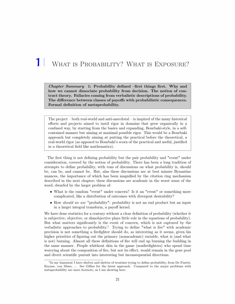
Figure 2.6: The "true" distributionas expected from the Monte Carlogenerator Shortfall

!6 !5 !4 !3 !2 !1x

0.2

0.4

0.6

0.8

p!x"

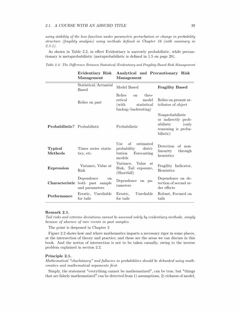
Figure 2.7: A typical realization,that is, an observed distribution forN = 103

!5 !4 !3 !2 !1 0

50

100

150

200

250

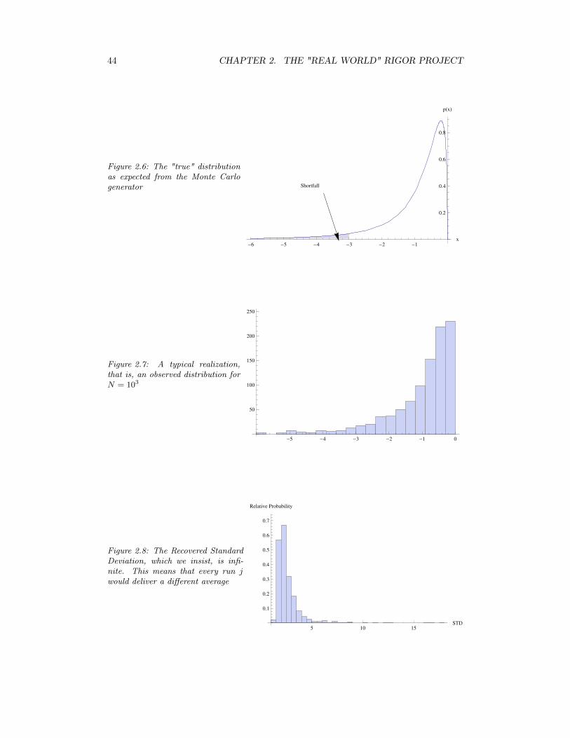
Figure 2.8: The Recovered StandardDeviation, which we insist, is infi-nite. This means that every run jwould deliver a different average

5 10 15STD

0.1

0.2

0.3

0.4

0.5

0.6

0.7

Relative Probability


Table 2.3: General Rules of Risk Engineering

Rules Description

R1 Dutch Book Probabilities need to add up to 1* � but cannot ex-ceed 1

R1

0Inequalities It is more rigorous to work with probability inequal-

ities and bounds than probabilistic estimates.

R2 Asymmetry Some errors have consequences that are largely, andclearly one sided.**

R3 Nonlinear Response Fragility is more measurable than probability***

R4 Conditional Pre-cautionary Princi-ple

Domain specific precautionary, based on fat tailed-ness of errors and asymmetry of payoff.

R5 Decisions Exposures (f(x))can be more reliably modified, in-stead of relying on computing probabilities of x.

* The Dutch book can be expressed, using the spirit of quantitative finance, as a no arbitragesituation, that is, no linear combination of payoffs can deliver a negative probability or onethat exceeds 1. This and the corrollary that there is a non-zero probability of visible andknown states spanned by the probability distribution adding up to <1 confers to probabilitytheory, when used properly, a certain analytical robustness.

** Consider a plane ride. Disturbances are more likely to delay (or worsen) the flight thanaccelerate it or improve it. This is the concave case. The opposite is innovation and tinkering,the convex case.

*** The errors in measuring nonlinearity of responses are more robust and smaller than thosein measuring responses. (Transfer theorems).

underestimate the "tail risk" below 1% and 99% for more severe risks. This exercisewas a standard one but there are many more complicated distributions than the ones weplayed with.

2.2.2 Good News: Five General Rules for Real World DecisionTheory

Table 2.3 provides a robust approach to the problem.

The good news is that the real world is about exposures, and exposures are asymmetric,leading us to focus on two aspects: 1) probability is about bounds, 2) the asymmetryleads to convexities in response, which is the focus of this text. Note that, thanks toinequalities and bounds (some tight, some less tight), the use of the classical theoremsof probability theory can lead to classes of qualitative precautionary decisions that,ironically, do not rely on the computation of specific probabilities.


The Supreme Scientific Rigor of The Russian School of Prob-ability

One can believe in the rigor of mathematical statements about probability withoutfalling into the trap of providing naive computations subjected to model error. Ifthis author were to belong to a school of thought designated by a nationality, the

{Nationality} school of {discipline},it would be the Russian school of probability.Members across three generations: P.L. Chebyshev, A.A. Markov, A.M. Lyapunov,S.N. Bernshtein (ie. Bernstein), E.E. Slutskii, N.V. Smirnov, L.N. Bol’shev, V.I.Romanovskii, A.N. Kolmogorov, Yu.V. Linnik, and the new generation: V. Petrov,A.N. Nagaev, A. Shyrayev, and a few more.They had something rather potent in the history of scientific thought: they thoughtin inequalities, not equalities (most famous: Markov, Chebyshev, Bernstein, Lya-punov). They used bounds, not estimates. Even their central limit version wasa matter of bounds, which we exploit later by seeing what takes place outside thebounds. They were world apart from the new generation of users who think in termsof precise probability –or worse, mechanistic social scientists. Their method accom-modates skepticism, one-sided thinking: "A is > x, AO(x) [Big-O: "of order" x],rather than A = x.For those working on integrating the mathematical rigor in risk bearing they providea great source. We always know one-side, not the other. We know the lowest valuewe are willing to pay for insurance, not necessarily the upper bound (or vice versa).a

aThe way this connects to robustness, which we will formalize next section, is as follows. Isrobust what does not change across perturbation of parameters of the probability distribution; thisis the core of the idea in Part II with our focus on fragility and antifragility. The point is refinedwith concave or convex to such perturbations.

2.3 Fragility, not Just Statistics, For Hidden Risks

Let us start with a sketch of the general solution to the problem of risk and probability,just to show that there is a solution (it will take an entire book to get there). Thefollowing section will outline both the problem and the methodology.

This reposes on the central idea that an assessment of fragility �and control of suchfragility�is more ususeful, and more reliable,than probabilistic risk management anddata-based methods of risk detection.

In a letter to Nature about the book Antifragile[77]: Fragility (the focus of PartII of this volume) can be defined as an accelerating sensitivity to a harmful stressor:this response plots as a concave curve and mathematically culminates in more harmthan benefit from the disorder cluster: (i) uncertainty, (ii) variability, (iii) imperfect,incomplete knowledge, (iv) chance, (v) chaos, (vi) volatility, (vii) disorder, (viii) entropy,(ix) time, (x) the unknown, (xi) randomness, (xii) turmoil, (xiii) stressor, (xiv) error,(xv) dispersion of outcomes, (xvi) unknowledge.

Antifragility is the opposite, producing a convex response that leads to more benefitthan harm. We do not need to know the history and statistics of an item to measure itsfragility or antifragility, or to be able to predict rare and random (’Black Swan’) events.All we need is to be able to assess whether the item is accelerating towards harm orbenefit.

Same with model errors –as we subject models to additional layers of uncertainty.

2.3. FRAGILITY, NOT JUST STATISTICS, FOR HIDDEN RISKS 47

Figure 2.9: The risk of breakingof the coffee cup is not necessar-ily in the past time series of thevariable; in fact surviving ob-jects have to have had a "rosy"past. Further, fragilefragile ob-jects are disproportionally morevulnerable to tail events than or-dinary ones –by the concavityargument.

The relation of fragility, convexity and sensitivity to disorder is thus mathematicaland not derived from empirical data.

The problem with risk management is that "past" time series can be (and actuallyare) unreliable. Some finance journalist was commenting on the statement in Antifragileabout our chronic inability to get the risk of a variable from the past with economic timeseries, with associated overconfidence. "Where is he going to get the risk from sincewe cannot get it from the past? from the future?", he wrote. Not really, it is staringat us: from the present, the present state of the system. This explains in a way whythe detection of fragility is vastly more potent than that of risk –and much easier todo. We can use the past to derive general statistical statements, of course, coupled withrigorous probabilistic inference but it is unwise to think that the data unconditionallyyields precise probabilities, as we discuss next.

Asymmetry and Insufficiency of Past Data. Our focus on fragility doesnot mean you can ignore the past history of an object for risk management, it is justaccepting that the past is highly insufficient.

The past is also highly asymmetric. There are instances (large deviations) for whichthe past reveals extremely valuable information about the risk of a process. Somethingthat broke once before is breakable, but we cannot ascertain that what did not break isunbreakable. This asymmetry is extremely valuable with fat tails, as we can reject sometheories, and get to the truth by means of negative inference, via negativa.

This confusion about the nature of empiricism, or the difference between empiri-cism (rejection) and naive empiricism (anecdotal acceptance) is not just a problem withjournalism. As we will see in Chapter x, it pervades social science and areas of sciencesupported by statistical analyses. Yet naive inference from time series is incompatiblewith rigorous statistical inference; yet many workers with time series believe that it isstatistical inference. One has to think of history as a sample path, just as one looksat a sample from a large population, and continuously keep in mind how representativethe sample is of the large population. While analytically equivalent, it is psychologicallyhard to take what Daniel Kahneman calls the "outside view", given that we are all partof history, part of the sample so to speak.

Let us now look at the point more formally, as the difference between an assessment


of fragility and that of statistical knowledge can be mapped into the difference betweenx and f(x)

This will ease us into the "engineering" notion as opposed to other approaches todecision-making.

2.3.1 The Solution: Convex Heuristic

Next we give the reader a hint of the methodology and proposed approach with a semi-informal technical definition for now.

In his own discussion of the Borel-Cantelli lemma (the version popularly known as"monkeys on a typewriter")[8], Emile Borel explained that some events can be consideredmathematically possible, but practically impossible. There exists a class of statementsthat are mathematically rigorous but practically nonsense, and vice versa.

If, in addition, one shifts from "truth space" to consequence space", in other wordsfocus on (a function of) the payoff of events in addition to probability, rather than justtheir probability, then the ranking becomes even more acute and stark, shifting, as wewill see, the discussion from probability to the richer one of fragility. In this book wewill include costs of events as part of fragility, expressed as fragility under parameterperturbation. Chapter 5 discusses robustness under perturbation or metamodels (ormetaprobability). But here is the preview of the idea of convex heuristic, which in plainEnglish, is at least robust to model uncertainty.

Definition 2.5 (Convex Heuristic).In short what exposure is required to not produce concave responses under parameterperturbation.

Summary of a Convex Heuristic (from Chapter 16) Let {fi} be the familyof possible functions, as "exposures" to x a random variable with probability mea-sure ��

(x), where �� is a parameter determining the scale (say, mean absolutedeviation) on the left side of the distribution (below the mean). A decision rule issaid "nonconcave" for payoff below K with respect to �� up to perturbation � if,taking the partial expected payoff

EK��(fi) =

Z K

�1fi(x) d��

(x),

fi is deemed member of the family of convex heuristics Hx,K,��,�,etc.:

⇢

fi :1

2

✓

EK��

(fi) + EK��

+�

(fi)

◆

� EK��(fi)

�

Note that we call these decision rules "convex" in H not necessarily because they havea convex payoff, but also because, thanks to the introduction of payoff f , their payoffends up comparatively "more convex" than otherwise. In that sense, finding protectionis a convex act.

Outline of Properties (nonmathematical) of Convex Heuristics Their aimis not to be "right" and avoid errors, but to ensure that errors remain small inconsequences.Definition 2.6.

2.4. FRAGILITY AND MODEL ERROR 49

A convex heuristic is a decision rule with the following properties:(a) Compactness: It is easy to remember, implement, use, and transmit.(b) Consequences, not truth: It is about what it helps you do, not whether it is

true or false. It should be judged not in "truth space" but in "consequence space."(c) Antifragility: It is required to have a benefit when it is helpful larger than the

loss when it is harmful. Thus it will eventually deliver gains from disorder.(d) Robustness: It satisfies the fragility-based precautionary principle.(e) Opacity: You do not need to understand how it works.(f) Survivability of populations: Such a heuristic should not be judged solely on its

intelligibility (how understandable it is), but on its survivability, or on a combinationof intelligibility and survivability. Thus a long-surviving heuristic is less fragilefragilethan a newly emerging one. But ultimately it should never be assessed in its survivalagainst other ideas, rather on the survival advantage it gave the populations who usedit.

The idea that makes life easy is that we can capture model uncertainty (and modelerror) with simple tricks, namely the scale of the distribution.

2.4 Fragility and Model Error

Crucially, we can gauge the nonlinear response to a parameter of a model using the samemethod and map "fragility to model error". For instance a small perturbation in theparameters entering the probability provides a one-sided increase of the likelihood ofevent (a convex response), then we can declare the model as unsafe (as with the assess-ments of Fukushima or the conventional Value-at-Risk models where small parametersvariance more probabilities by 3 orders of magnitude). This method is fundamentallyoption-theoretic.

2.4.1 Why Engineering?

[Discussion of the problem- A personal record of the difference between measurementand working on reliability. The various debates.]

2.4.2 Risk is not Variations

On the common confustion between risk and variations. Risk is tail events, necessarily.

2.4.3 What Do Fat Tails Have to Do With This?

The focus is squarely on "fat tails", since risks and harm lie principally in the high-impact events, The Black Swan and some statistical methods fail us there. But theydo so predictably. We end Part I with an identification of classes of exposures to theserisks, the Fourth Quadrant idea, the class of decisions that do not lend themselves tomodelization and need to be avoided � in other words where x is so reliable that oneneeds an f(x) that clips the left tail, hence allows for a computation of the potentialshortfall. Again, to repat, it is more, much more rigorous to modify your decisions.


2.4.4 Fat Tails and Model Expansion

Next wee see how model uncertainty (or, within models, parameter uncertainty), ormore generally, adding layers of randomness, cause fat tails. Part I of this volumepresents a mathematical approach for dealing with errors in conventional probabilitymodels For instance, if a "rigorously" derived model (say Markowitz mean variance, orExtreme Value Theory) gives a precise risk measure, but ignores the central fact thatthe parameters of the model don’ t fall from the sky, but have some error rate in theirestimation, then the model is not rigorous for risk management, decision making in thereal world, or, for that matter, for anything.

So we may need to add another layer of uncertainty, which invalidates some modelsbut not others. The mathematical rigor is therefore shifted from focus on asymptotic(but rather irrelevant because inapplicable) properties to making do with a certain setof incompleteness and preasymptotics. Indeed there is a mathematical way to deal withincompletness. Adding disorder has a one-sided effect and we can deductively estimateits lower bound. For instance we can figure out from second order effects that tailprobabilities and risk measures are understimated in some class of models.

2.4.5 Savage’s Difference Between The Small and Large World

Figure 2.10: A Version of Savage’s Small World/Large World Problem. In statistical domainsassume Small World= coin tosses and Large World = Real World. Note that measuretheory is not the small world, but large world, thanks to the degrees of freedom it confers.

The problem of formal probability theory is that it necessarily covers narrower situa-tions (small world ⌦S) than the real world (⌦L), which produces Procrustean bed effects.⌦S ⇢ ⌦L. The "academic" in the bad sense approach has been to assume that ⌦L is

2.4. FRAGILITY AND MODEL ERROR 51

smaller rather than study the gap. The problems linked to incompleteness of models arelargely in the form of preasymptotics and inverse problems.

Real world and "academic" don’t necessarily clash Luckily there is aprofound literature on satisficing and various decision-making heuristics, starting withHerb Simon and continuing through various traditions delving into ecological rationality,[69], [35], [80]: in fact Leonard Savage’s difference between small and large worlds willbe the basis of Part I, which we can actually map mathematically. Method: We cannotprobe the Real World but we can get an idea (via perturbations) of relevant directionsof the effects and difficulties coming from incompleteness, and make statements s.a. "in-completeness slows convergence to LLN by at least a factor of n↵”, or "increases thenumber of observations to make a certain statement by at least 2x".

So adding a layer of uncertainty to the representation in the form of model error, ormetaprobability has a one-sided effect: expansion of ⌦S with following results:

i) Fat tails:i-a)- Randomness at the level of the scale of the distribution generates fat tails.(Multi-level stochastic volatility).i-b)- Model error in all its forms generates fat tails.i-c) - Convexity of probability measures to uncertainty causes fat tails.ii) Law of Large Numbers(weak): operates much more slowly, if ever at all. "P-values" are biased lower.iii) Risk is larger than the conventional measures derived in ⌦S , particularly forpayoffs in the tail.iv) Allocations from optimal control and other theories (portfolio theory) have ahigher variance than shown, hence increase risk.v) The problem of induction is more acute.(epistemic opacity).vi)The problem is more acute for convex payoffs, and simpler for concave ones.

Now i) ) ii) through vi).

Risk (and decisions) require more rigor than other applications of statistical inference.

2.4.6 Coin tosses are not quite "real world" probability

In his wonderful textbook [10], Leo Breiman referred to probability as having two sides,the left side represented by his teacher, Michel Loève, which concerned itself with formal-ism and measure theory, and the right one which is typically associated with coin tossesand similar applications. Many have the illusion that the "real world" would be closerto the coin tosses. It is not: coin tosses are fake practice for probability theory, artificialsetups in which people know the probability (what is called the ludic fallacy in TheBlack Swan), and where bets are bounded, hence insensitive to problems of extreme fattails. Ironically, measure theory, while formal, is less constraining and can set us freefrom these narrow structures. Its abstraction allows the expansion out of the small box,all the while remaining rigorous, in fact, at the highest possible level of rigor. Plenty ofdamage has been brought by the illusion that the coin toss model provides a "realistic"approach to the discipline, as we see in Chapter x, it leads to the random walk and theassociated pathologies with a certain class of unbounded variables.


2.5 General Classification of Problems Related To FatTails

The Black Swan Problem Incomputability of Small Probalility: It is is notmerely that events in the tails of the distributions matter, happen, play a large role, etc.The point is that these events play the major role for some classes of random variablesand their probabilities are not computable, not reliable for any effective use. And thesmaller the probability, the larger the error, affecting events of high impact. The ideais to work with measures that are less sensitive to the issue (a statistical approch), orconceive exposures less affected by it (a decision theoric approach). Mathematically, theproblem arises from the use of degenerate metaprobability.

In fact the central point is the 4

th quadrant where prevails both high-impact and non-measurability, where the max of the random variable determines most of the properties(which to repeat, has not computable probabilities).

We will rank probability measures along this arbitrage criterion.

Associated Specific "Black Swan Blindness" Errors (Applying Thin–Tailed Metrics to Fat Tailed Domains) These are shockingly common, aris-ing from mechanistic reliance on software or textbook items (or a culture of bad statisticalinsight).We skip the elementary "Pinker" error of mistaking journalistic fact - checkingfor scientific statistical "evidence" and focus on less obvious but equally dangerous ones.

1. Overinference: Making an inference from fat-tailed data assuming sample sizeallows claims (very common in social science). Chapter 3.

2. Underinference: Assuming N=1 is insufficient under large deviations. Chapters1 and 3.

(In other words both these errors lead to refusing true inference and acceptinganecdote as "evidence")

3. Asymmetry: Fat-tailed probability distributions can masquerade as thin tailed("great moderation", "long peace"), not the opposite.

4. The econometric ( very severe) violation in using standard deviations and variancesas a measure of dispersion without ascertaining the stability of the fourth moment(F .F ) . This error alone allows us to discard everything in economics/econometricsusing � as irresponsible nonsense (with a narrow set of exceptions).

5. Making claims about "robust" statistics in the tails. Chapter 3.

6. Assuming that the errors in the estimation of x apply to f(x) ( very severe).

7. Mistaking the properties of "Bets" and "digital predictions" for those of Vanillaexposures, with such things as "prediction markets". Chapter 9.

8. Fitting tail exponents power laws in interpolative manner. Chapters 2, 6

9. Misuse of Kolmogorov-Smirnov and other methods for fitness of probability distri-bution. Chapter 3.

10. Calibration of small probabilities relying on sample size and not augmenting thetotal sample by a function of 1/p , where p is the probability to estimate.

11. Considering ArrowDebreu State Space as exhaustive rather than sum of knownprobabilities 1

2.6. CLOSING THE INTRODUCTION 53

Problem Description Chapters

1 Preasymptotics,Incomplete Conver-gence

The real world is before the asymptote.This affects the applications (under fattails) of the Law of Large Numbers andthe Central Limit Theorem.

?

2 Inverse Problems a) The direction Model ) Reality pro-duces larger biases than Reality )

Model

b) Some models can be "arbitraged" inone direction, not the other .

1,?,?

3 DegenerateMetaprobability*

Uncertainty about the probability dis-tributions can be expressed as addi-tional layer of uncertainty, or, simpler,errors, hence nested series of errors onerrors. The Black Swan problem can besummarized as degenerate metaproba-bility.2

?,?

*Degenerate metaprobability is a term used to indicate a single layer of stochasticity,such as a model with certain parameters.

2.6 Closing the Introduction

We close the introduction with De Finetti’s introduction to his course "On Probability":The course, with a deliberately generic title will deal with the conceptual and

controversial questions on the subject of probability: questions which it is necessaryto resolve, one way or another, so that the development of reasoning is not reducedto a mere formalistic game of mathematical expressions or to vacuous and simplisticpseudophilosophical statements or allegedly practical claims. (emph. mine.)

The next appendix deplores academic treatment of probability so we get it out of theway.

A What’s a Charlatan in Risk andProbability?

We start with a clean definition of charlatan. Many of us spend time fighting withcharlatans; we need a cursory and useable definition that is both compatible with ourprobability business and the historical understanding of the snake-oil salesman.

A.1 Charlatan

Definition A.1.Charlatan In our context someone who meets at least two of the following. He

a) proposes complicated practical solutions to a problem that may or may not exist orhas a practical simpler and less costly alternative

b) favors unconditional via positiva over via negativa

c) has small or no offsetting exposure to iatrogenics1, in a way to incur no or minimalharm should the solution to the problem be worse than doing nothing

d) avoids nonlucrative or career-enhancing solutions

e) does not take professional, reputational or financial risks for his opinion

f) in assessments of small probability, tends to produces a number rather than a lowerbound

g) tries to make his audience confuse "absence of evidence" for "evidence of absence"with small probability events.

Remark A.1.A charlatan is the exact opposite of the skeptic or skeptical empiricist.

(The skeptical empiricist is traditionally, contrary to casual descriptions, someone whoputs a high burden on empirical data and focuses on the unknown, the exact oppositeto the naive empiricist.)

Remark A.2.Our definition of charlatan isn’t about what he knows, but the ratio of iatrogenics in theconsequences of his actions.

1Iatrogenics is harm caused by the healer

55

56 APPENDIX A. WHAT’S A CHARLATAN IN RISK AND PROBABILITY?

The GMO Problem For instance we can spot a difficulty by the insistence bysome "scientists" on the introduction of genetically modified "golden rice" with addedvitamins as a complicated solution to some nutritional deficiency to "solve the problem"when simpler solutions (with less potential side effects) are on hand are available (suchas to just give the people vitamin pills).

The charlatan can be highly credentialed (with publications in Econometrica) or merelyone of those risk management consultants. A mathematician may never be a charlatanwhen doing math, but becomes one automatically when proposing models full of iatro-genics and imposing them uncritically to reality. We will see how charlatans operate byimplicit collusion using citation rings.

A.1.1 Citation Rings and Cosmetic Job Market Science

Subdiscipline of Bullshit-tology I am being polite here.I truly believe that a scaryshare of current discussions ofrisk management and prob-ability by nonrisktakers fallinto the category called ob-scurantist, partaking of the"bullshitology" discussed inElster: "There is a less politeword for obscurantism: bull-shit. Within Anglo-Americanphilosophy there is in facta minor sub-discipline thatone might call bullshittology."[21]. The problem is that,because of nonlinearities withrisk, minor bullshit can leadto catastrophic consequences,just imagine a bullshitter pi-loting a plane. My angleis that the bullshit-cleaner inthe risk domain is skin-in-the-game, which eliminates thosewith poor understanding ofrisk.

Citation rings are how charlatans can operateas a group. All members in citations rings arenot necessarily charlatans, but group charla-tans need citation rings.

How I came about citation rings? At a cer-tain university a fellow was being evaluatedfor tenure. Having no means to gauge his im-pact on the profession and the quality of hisresearch, they checked how many "top publi-cations" he had. Now, pray, what does consti-tute a "top publication"? It turned out thatthe ranking is exclusively based on the cita-tions the journal gets. So people can form ofgroup according to the Latin expression asinusasimum fricat (donkeys rubbing donkeys), citeeach other, and call themselves a discipline oftriangularly vetted experts.

Detecting a "clique" in network theory is howterrorist cells and groups tend to be identifiedby the agencies.

Now what if the fellow got citations on hisown? The administrators didn’t know how tohandle it.

Looking into the system revealed quite a bitof arbitrage-style abuse by operators.

Definition A.2.Higher order self-referential system. Ai

references Aj 6=i, Aj references Az 6=j, · · ·, Az references Ai.

Definition A.3.Academic Citation Ring A legal higher-order self-referential collection of operatorswho more or less "anonymously" peer-review and cite each other, directly, triangularly,or in a network manner, constituting a clique in a larger network, thus creating so-calledacademic impact ("highly cited") for themselves or their journals.

Citation rings become illegal when operators use fake identities; they are otherwise legalno matter how circular the system.

A.1. CHARLATAN 57


PracticeReal Life

(B)Math/Logic (C)

C � A' � B'

Figure A.1: The Triffat Fallacy,or the way academic decision theoryand mathematical statistics view de-cision, probability, and risk.a

aFor an example of Byzantine con-cerns about probability so detailed anddiverted from planet earth that theymiss everything of relevance to risk, seethe works of David Aldous on the cen-tral difference between "finite additiv-ity" or "countable additivity", whichcan be classified as the hijacking of themost important discipline in the world,probability, by scholastic distinctionswithout (or with relatively minor) real-world difference.

The mark of such system is engagement in incremental science in a given direction,calling each other’s results "innovative". Example of dangerous citation ring: Markowitzmean-variance, GARCH, Value-At-Risk and more general risk management, some tradi-tions of behavioral economics.

Definition A.4.Job Market Science A paper that follows recipes and tricks to attain higher rankingin a certain community. It seems a "contribution" but it is explained by connection toother parts which are triangularly self-referential ; it is otherwise substance-free.

Take GARCH methods (Rob Engle [26]): we know that, in practice, GARCH is totallyuseless to predict volatility; it is an academic PR machine. And, analytically, it isunsound under the structure of fat tails in the markets, as we will see in Chapter 3 andsection 7.11 But the "Nobel" plus an active citation ring deems it a "successful" theory.

It is clear that, with rare exceptions articles published Econometrica are either substance-free or pure distortion (use of variance as measure of variability).

How do we break away from substance-free statistical science? Skin in the game, ofcourse, reestablishes contact with reality, with details in Chapter 14 . The central ideais that survival matters in risk, people not truly exposed to harm can continue operatingpermanently.

A.1.2 The Triffat Fallacy

An illustration of our nighmare for risk management –and an explanation of why wecan’t accept current methods in economics for anything to do with the real world – is asfollows. From Antifragile[77]:

Modern members of the discipline of decision theory, alas, travel a one- way roadfrom theory to practice. They characteristically gravitate to the most complicatedbut most inapplicable problems, calling the process "doing science."

There is an anecdote about one Professor Triffat (I am changing the name be-cause the story might be apocryphal, though from what I have witnessed, it isvery characteristic). He is one of the highly cited academics of the field of decisiontheory, wrote the main textbook and helped develop something grand and uselesscalled "rational decision making," loaded with grand and useless axioms and shmax-ioms, grand and even more useless probabilities and shmobabilities. Triffat, then at

58 APPENDIX A. WHAT’S A CHARLATAN IN RISK AND PROBABILITY?

Columbia University, was agonizing over the decision to accept an appointment atHarvard –many people who talk about risk can spend their lives without encoun-tering more difficult risk taking than this type of decision. A colleague suggestedhe use some of his Very Highly Respected and Grandly Honored and Decoratedacademic techniques with something like "maximum expected utility," as, he toldhim, "you always write about this." Triffat angrily responded, "Come on, this isserious!"

Definition A.5.The Triffat Fallacy. Consists in confusing the problem and the inverse problem, goingfrom theory to practice, at the intersection C \A0

\B0 according to definitions in A.1.2.There has been a lot of trivial commentary, a recurring critique of theoretical risk

management, (with the person feeling that he has just discovered it): things are "toomathematical", "mathematics does not work in the real world", or lists of what doesor does not constitute "mathematical charlatanry".2 But little or nothing seems to bedone to figure out where math works and is needed; where standard methods ascribed toscience, whether evidentiary (statistics) or analytical (mathematics/logic) do not applyin Risk management and decision making under opacity –since one doesn’t have thewhole story– except as constraints.

Pseudo-Rigor and Lack of skin in the game The disease of pseudo-rigor in theapplication of probability to real life by people who are not harmed by their mistakescan be illustrated as follows, with a very sad case study. One of the most "cited"document in risk and quantitative methods is about "coherent measures of risk",which set strong rules on how to compute tail risk measures, such as the "valueat risk" and other methods. Initially circulating in 1997, the measures of tail risk�while coherent� have proven to be underestimating risk at least 500 million times(sic). We have had a few blowups since, including Long Term Capital Managementfiasco �and we had a few blowups before, but departments of mathematical prob-ability were not informed of them. As we are writing these lines, it was announcedthat J.-P. Morgan made a loss that should have happened every ten billion years.The firms employing these "risk minds" behind the "seminal" paper blew up andended up bailed out by the taxpayers. But we now now about a "coherent measureof risk". This would be the equivalent of risk managing an airplane flight by spend-ing resources making sure the pilot uses proper grammar when communicatingwith the flight attendants, in order to "prevent incoherence". Clearly the problem,just as similar fancy "science" under the cover of the discipline of Extreme ValueTheory is that tail events are very opaque computationally, and that such misplacedprecision leads to confusion.a

aThe "seminal" paper: Artzner, P., Delbaen, F., Eber, J. M., & Heath, D. (1999), Coherentmeasures of risk. [1]

2It has been fashionable to invoke the vague idea of mathematical "charlatanry" in the history ofeconomics, first with Alfred Marshall famous procedure "(1) Use mathematics as shorthand language,rather than as an engine of inquiry. (2) Keep to them till you have done. (3) Translate into English. (4)Then illustrate by examples that are important in real life (5) Burn the mathematics. (6) If you can’tsucceed in 4, burn 3. This I do often.".Similarly, J.M. Keynes: "(...)we will endeavour to discredit the mathematical charlatanry by which, fora hundred years past, the basis of theoretical statistics have been greatly undermined", in A TreatiseOn Probability [41]. As one can see, these types of warnings proved ineffectual owing to citation rings.So our tack is different, largely constrained by the idea of skin in the game that would bring things tothe missing link of reality.

A.2. THE "DÉJA VU" ILLUSION 59

A.2 The "Déja Vu" Illusion

A matter of some gravity. Black Swan neglect was prevalent before... and after theexposition of the ideas. They just feel as if they were present in the discourse. Forthere is a common response to the Black Swan problem, one of the sort: "fat tails...we know it. There is nothing new there". In general, the "nothing new" response ismore likely to come from nonspecialists or people who do not know a subject well.For a philistine, Verdi’s Trovatore is not new, since it sounds like another opera heheard by Mozart with women torturing their throat. One needs to know a subjectto place it in context.

We take a stop and show what is different in this text, and why it is a hindrance forrisk understanding. Our point point is that under fat tails we have near-total opacity forsome segments of the distribution, incomputability of tail probability and convergenceof different laws, hence need to move to measurements of fragility.

The response: "Mandelbrot and Pareto did fat tails" is effectively backwards. In factthey arrived to the opposite of opacity. Now, risk and uncertainty? Keynes and Knightdealt with uncertainty as opposed to risk? Well, they got exactly opposite results.

They do not notice that it is the equivalent of saying that anyone using an equa-tion is doing nothing new since equations were discovered by ancients, or that calculuswas invented by Newton, and that, accordingly, they themselves did nothing worthy ofattention.

Now, what they do not say "nothing new" about is exactly what has nothing new,some wrinkle on some existing conversation, by the narcissim of small differences.

Some economists’ reaction to skin-in-the-game, SITG (on which, later, but the biasis relevant here): "nothing new; we know everything about the agency problem" (re-markably they always know everything about everything but never see problems beforethey occur, and rarely after). Our point is beyond their standard agency problem: 1)it is evolutionary, aiming at throwing bad risk takers out of the gene pool so they stopharming others, 2) under fat tails, and slow law of large numbers, only SITG worksto protect systems, 3) It is moral philosophy, 4) It requires building a system that canaccommodate SITG. Economists do not notice that it is asking them to leave the poolwhen they make mistakes, etc. Effectively Joseph Stiglitz, the author of the Palgraveencyclopedia entry on the agency problem missed that had he had skin in the game withFanny Mae he would have exited the pool. Or before that, so we would have avoided abig crisis. If economists understood skin-in-the-game they would shut down many manysub-disciplines and stop giving macro advice. Giving opinions without downside is theopposite of SITG.

k t

Documents

dene probability

notion of probability

pair probability

equations of probability

probability dened

dening probability

variable x

clear denition of probability