Recommendation Systems

Kai Yu

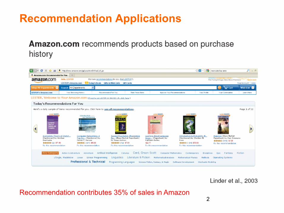
Recommendation Applications

2 Recommendation contributes 35% of sales in Amazon

Recommendation Applications

3

Recommendation Applications

4

Recommendation Applications

5

Outline

§  Problem definition §  Pre-processing §  CF as classification §  CF as matrix factorization §  Extensions §  Challenges

6

Collaborative filtering (CF)

7

Formal definition

8

CF as matrix completion

9

Metric

10

Outline

§  Problem definition §  Pre-processing §  CF as classification §  CF as matrix factorization §  Extensions §  Challenges

11

Pre-processing: centering data

12

Pre-processing: centering data

13

Intro Prelim Class/Reg MF Extend Combo Conclude Centering Shrinkage

Centering Your Data

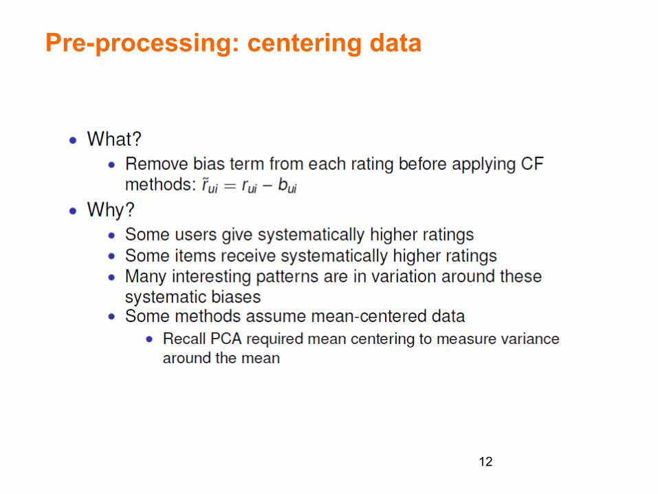
• What?• Remove bias term from each rating before applying CF

methods: r̃ui = rui � bui

• How?• Global mean rating

• bui =µ � 1|T |�

(u,i)⇤T rui

• Item’s mean rating• bui = bi � 1

|R(i)|�

u⇤R(i) rui

• R(i) is the set of users who rated item i• User’s mean rating

• bui = bu � 1|R(u)|

�i⇤R(u) rui

• R(u) is the set of items rated by user u• Item’s mean rating + user’s mean deviation from item mean

• bui = bi +1

|R(u)|�

i⇤R(u)(rui � bi)

Lester Mackey Collaborative Filtering

Shrinkage

14

Intro Prelim Class/Reg MF Extend Combo Conclude Centering Shrinkage

Shrinkage

• What?• Interpolating between an estimate computed from data and

a fixed, predetermined value• Why?

• Common task in CF: Compute estimate (e.g. a meanrating) for each user/item

• Not all estimates are equally reliable• Some users have orders of magnitude more ratings than

others• Estimates based on fewer datapoints tend to be noisier

R =

A B C D E F User meanAlice 2 5 5 4 3 5 4Bob 2 ? ? ? ? ? 2Craig 3 3 4 3 ? 4 3.4

• Hard to trust mean based on one rating

Lester Mackey Collaborative Filtering

Shrinkage

15

Intro Prelim Class/Reg MF Extend Combo Conclude Centering Shrinkage

Shrinkage

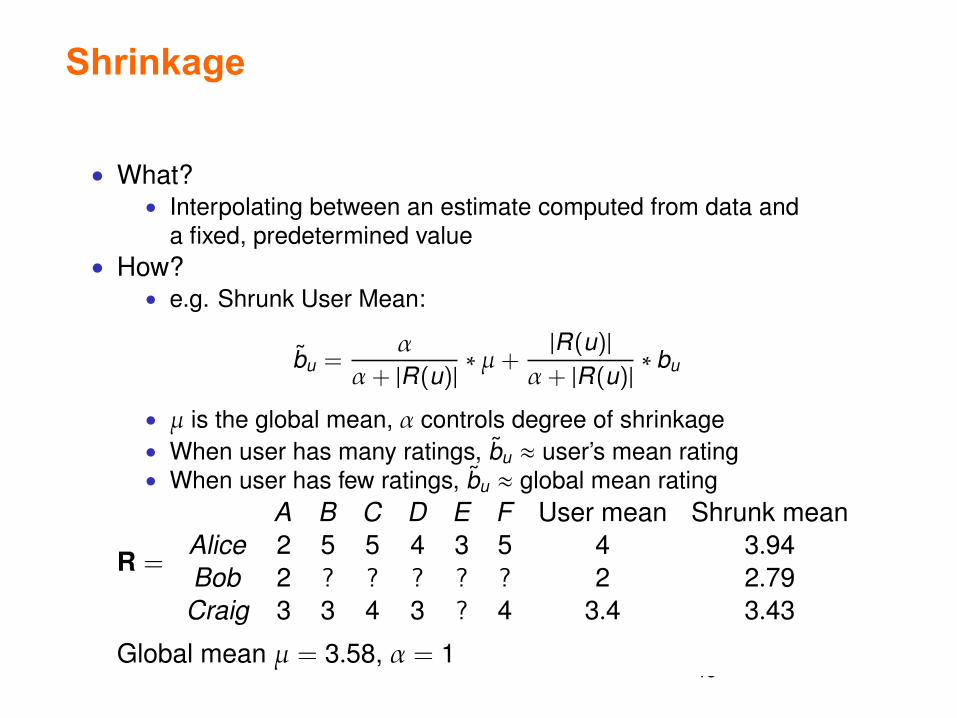
• What?• Interpolating between an estimate computed from data and

a fixed, predetermined value• How?

• e.g. Shrunk User Mean:

b̃u =�

�+ |R(u)| � µ+|R(u)|�+ |R(u)| � bu

• µ is the global mean, � controls degree of shrinkage• When user has many ratings, b̃u ⇤ user’s mean rating• When user has few ratings, b̃u ⇤ global mean rating

R =

A B C D E F User mean Shrunk meanAlice 2 5 5 4 3 5 4 3.94Bob 2 ? ? ? ? ? 2 2.79Craig 3 3 4 3 ? 4 3.4 3.43

Global mean µ = 3.58, � = 1

Lester Mackey Collaborative Filtering

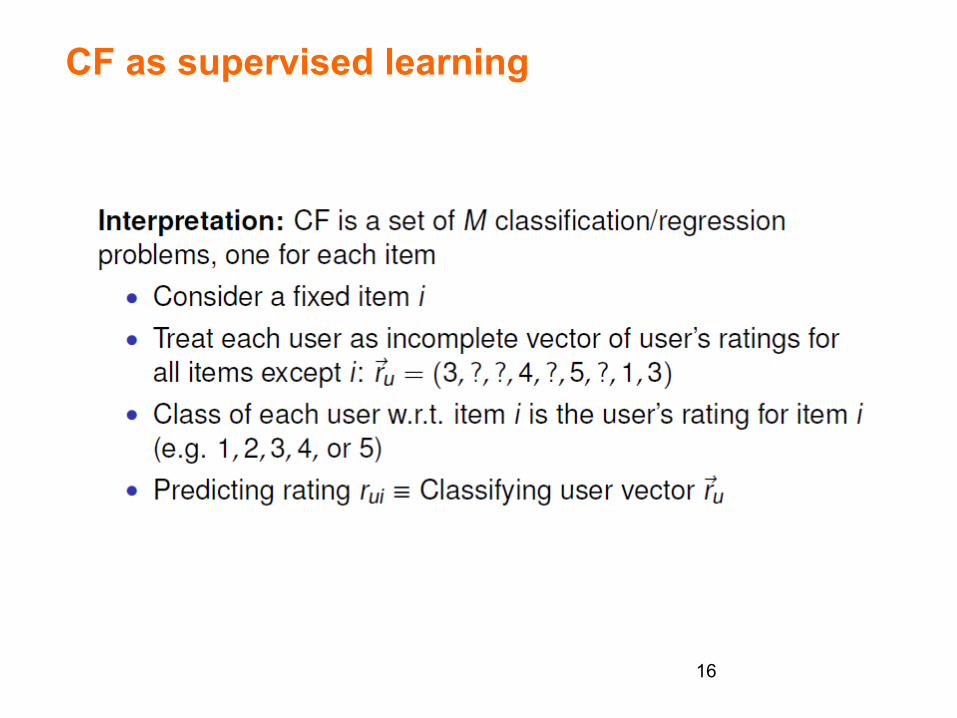
CF as supervised learning

16

CF as supervised leanring

17

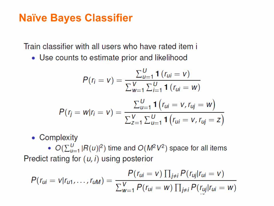
Naïve Bayes Classifier

18

Naïve Bayes Classifier

19

Naïve Bayes Classifier

20

KNN-based CF

21

KNN: how to measure similarity

22

Intro Prelim Class/Reg MF Extend Combo Conclude Naive Bayes KNN

KNN: Computing Similarities

How to measure similarity between items?• Cosine similarity

S(⇤r.i ,⇤r.j) =⇤⇤r.i ,⇤r.j⌅������⇤r.i������������⇤r.j������

• Pearson correlation coefficient

S(⇤r.i ,⇤r.j) =⇤⇤r.i �mean(⇤r.i),⇤r.j �mean(⇤r.j)⌅������⇤r.i �mean(⇤r.i)

������������⇤r.j �mean(⇤r.j)

������

• Inverse Euclidean distance

S(⇤r.i ,⇤r.j) =1���

���⇤r.i �⇤r.j������

Problem: These measures assume complete vectorsSolution: Compute over subset of users rated by both itemsComplexity: O(

⇥Uu=1 |R(u)|2) time

Herlocker et al., 1999Lester Mackey Collaborative Filtering

KNN: choosing K

23

Intro Prelim Class/Reg MF Extend Combo Conclude Naive Bayes KNN

KNN: Choosing K neighbors

How to choose K nearest neighbors?

• Select K items with largest similarity score to query item i

Problem: Not all items were rated by query user u

Solution: Choose K most similar items rated by u

Complexity: O(min(KM,M log M))

Herlocker et al., 1999

Lester Mackey Collaborative Filtering

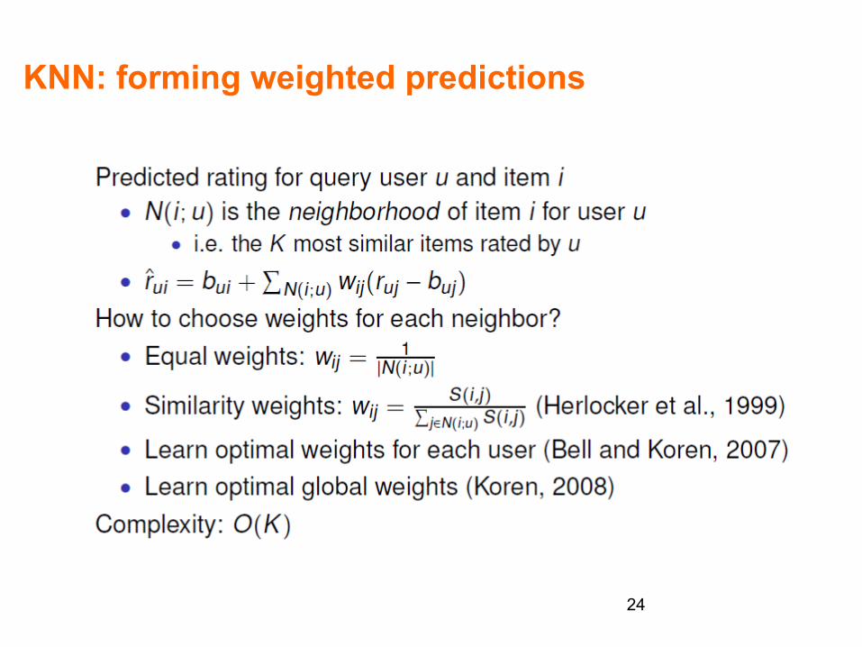
KNN: forming weighted predictions

24

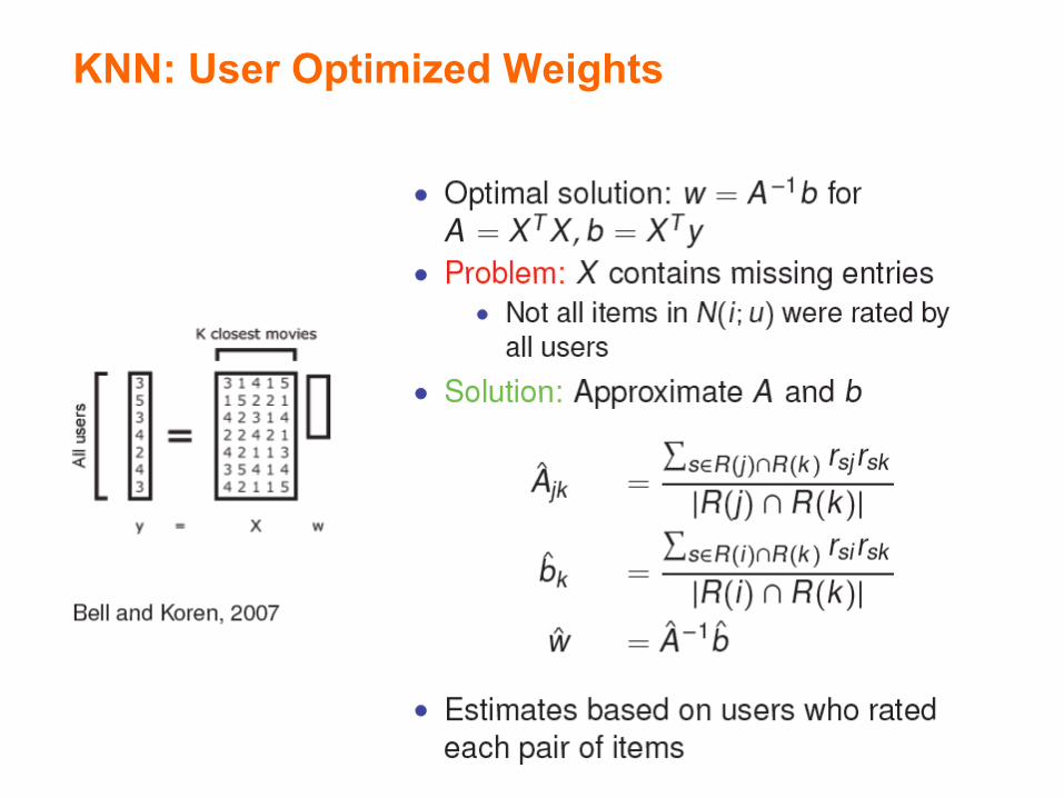
KNN: User Optimized Weights

25

KNN: User Optimized Weights

26

KNN: User Optimized Weights

27

KNN: globally optimized weights

28

KNN: globally optimized weights

29

Intro Prelim Class/Reg MF Extend Combo Conclude Naive Bayes KNN

KNN: Globally Optimized Weights

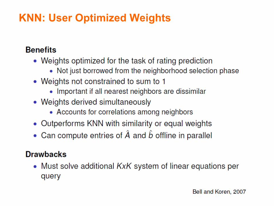
Benefits• Weights optimized for the task of rating prediction

• Not just borrowed from the neighborhood selection phase• Weights not constrained to sum to 1

• Important if all nearest neighbors are dissimilar• Weights derived simultaneously

• Accounts for correlations among neighbors• Outperforms KNN with similarity or equal weights

Drawbacks• Must solve global optimization problem at training time• Must store O(M2) weights in memory

Koren, 2008

Lester Mackey Collaborative Filtering

KNN Summary

30

Outline

§  Problem definition §  Pre-processing §  CF as classification §  CF as matrix factorization §  Extensions §  Challenges

31

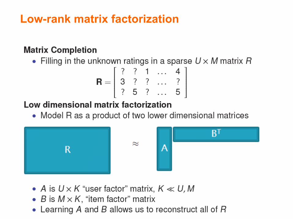
Low-rank matrix factorization

32

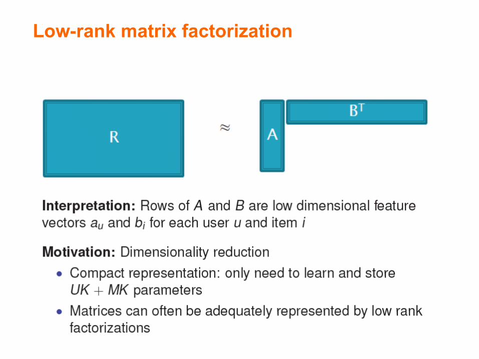
Low-rank matrix factorization

33

Singular Value Decomposition

34

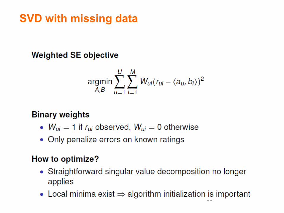
SVD with missing data

35

SVD with missing data

36

Regularization

37

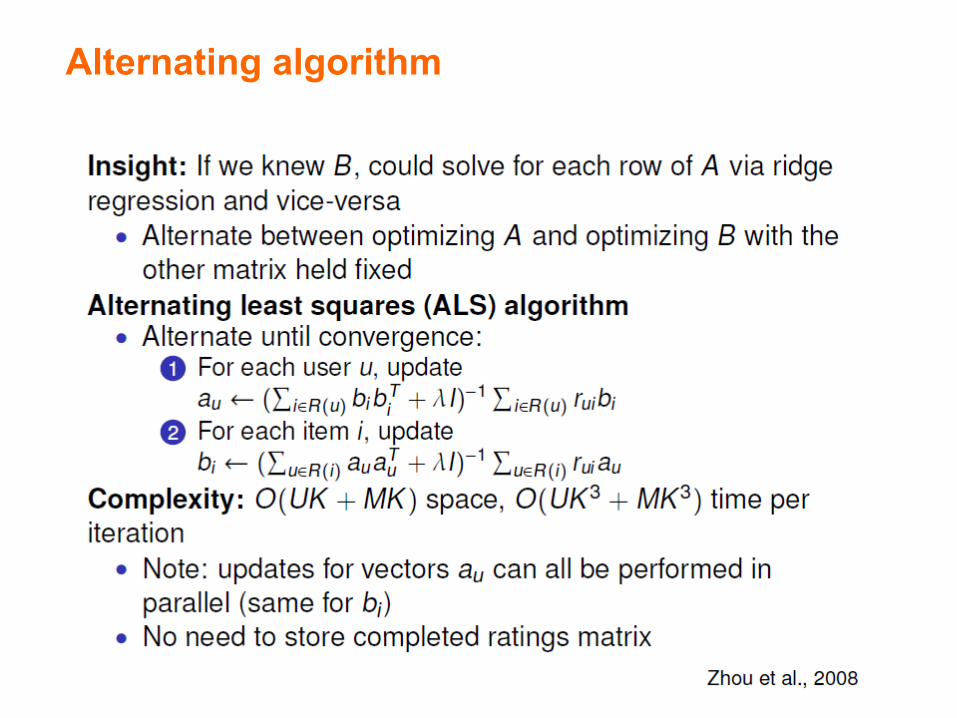
Alternating algorithm

38

Gradient descent algorithm

39

Stochastic gradient

40

Intro Prelim Class/Reg MF Extend Combo Conclude SVD Factor Analysis

SVD with Missing Values

Insight: Update parameter after each observed rating• ⇧auEui = ⇥au + bi(⌥au,bi� � rui)

• ⇧bi Eui = ⇥bi + au(⌥au,bi� � rui)

Stochastic gradient descent algorithm• Repeat until convergence:

1 For each (u, i) ⌅ T1 Calculate error: eui ⇤ (⌥au,bi� � rui)2 Update au ⇤ au � �(⇥au + bieui)3 Update bi ⇤ bi � �(⇥bi + aueui)

Complexity: O(UK + MK) space, O(NK) time per passthrough training set• No need to store completed ratings matrix• No K3 overhead from solving linear regressions

Takacs et al., 2008, Funk, 2006

Lester Mackey Collaborative Filtering

Constrained MF as clustering

41

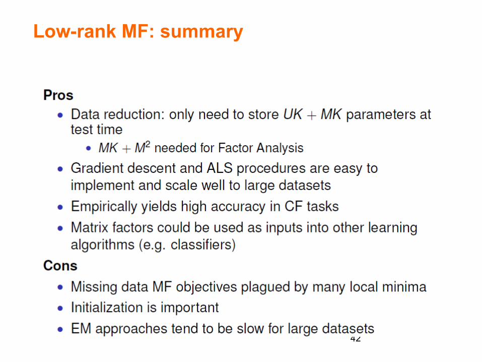
Low-rank MF: summary

42

Outline

§  Problem definition §  Pre-processing §  CF as classification §  CF as matrix factorization §  Extensions §  Challenges

43

Implicit feedback

44

Intro Prelim Class/Reg MF Extend Combo Conclude Implicit Feedback Time Dependence

Incorporating Implicit Feedback

Implicit feedback• In addition to explicitly observed ratings, may have access

to binary information reflecting implicit user preferences• Is a movie in a user’s queue at Netflix?• Was this item purchased (but never rated)?

• Test set can be a source of implicit feedback• For each (u, i) in the test set, we know u rated i; we just

don’t know the rating.• Data is not “missing at random”• The fact that a user rated an item provides information

about the rating.• E.g. People who rated Lord of The Rings I and II tend to rate

LOTR III more highly.

• Can extend several of our algorithms to incorporate implicitfeedback as additional binary preferences

Lester Mackey Collaborative Filtering

Incorporating implicit feedback

45

46

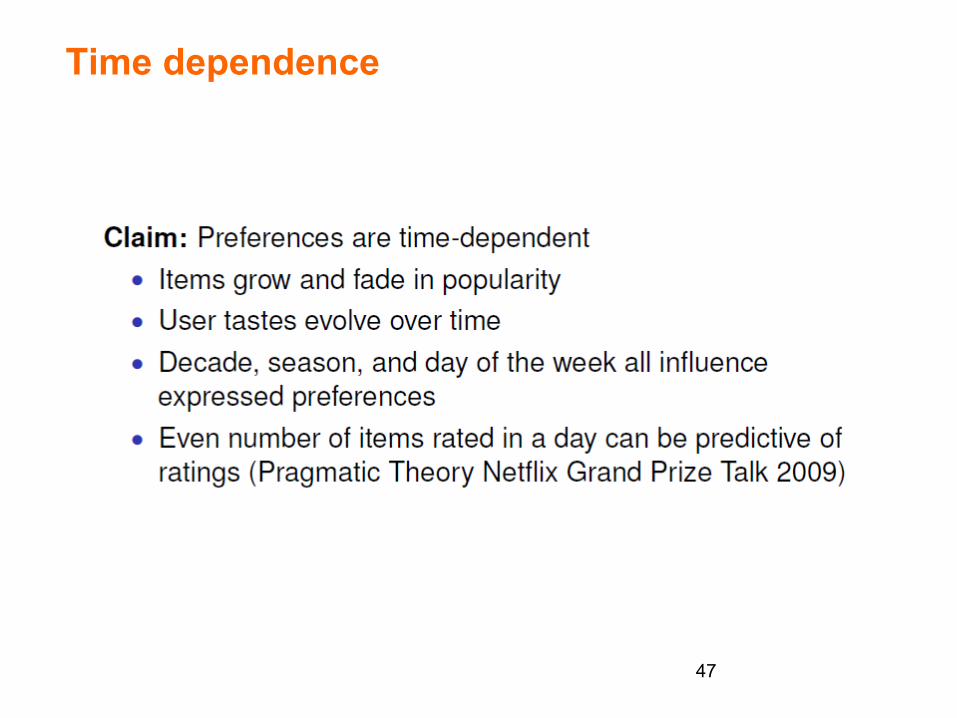
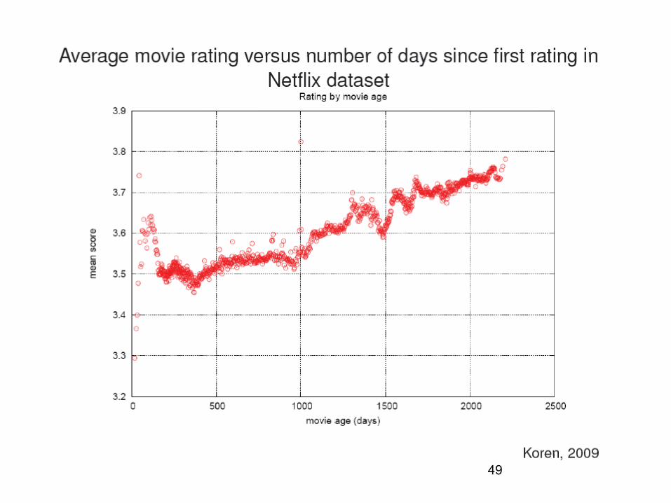
Time dependence

47

48

49

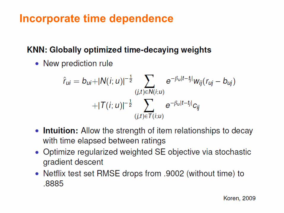
Incorporate time dependence

50

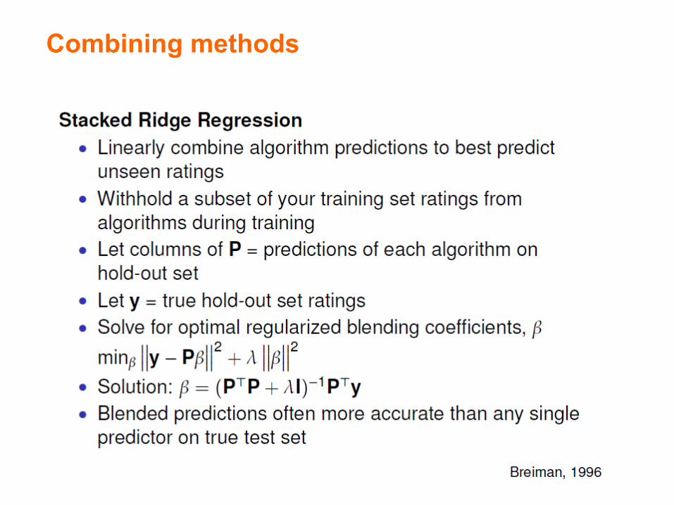
Combining methods

51

Combining methods

52

Combining methods

53

Outline

§  Problem definition §  Pre-processing §  CF as classification §  CF as matrix factorization §  Extensions §  Challenges

54

Challenges for CF

55

Challenges for CF

56

Challenges for CF

57