kalman filtering over gilbert–elliott channels: stability

IEEE TRANSACTIONS ON AUTOMATIC CONTROL, VOL. 63, NO. 4, APRIL 2018 1003

Kalman Filtering Over Gilbert–Elliott Channels:Stability Conditions and Critical Curve

Junfeng Wu , Guodong Shi , Brian D. O. Anderson , Life Fellow, IEEE,and Karl Henrik Johansson , Fellow, IEEE

Abstract—This paper investigates the stability of Kalmanfiltering over Gilbert–Elliott channels where random packetdrops follow a time-homogeneous two-state Markov chainwhose state transition is determined by a pair of failure andrecovery rates. First of all, we establish a relaxed conditionguaranteeing peak-covariance stability described by an in-equality in terms of the spectral radius of the system matrixand transition probabilities of the Markov chain. We furthershow that the condition can be interpreted using a linearmatrix inequality feasibility problem. Next, we prove thatthe peak-covariance stability implies mean-square stability,if the system matrix has no defective eigenvalues on theunit circle. This connection between the two stability no-tions holds for any random packet drop process. We provethat there exists a critical curve in the failure-recovery rateplane, below which the Kalman filter is mean-square stableand no longer mean-square stable above. Finally, a lowerbound for this critical failure rate is obtained making useof the relationship we establish between the two stabilitycriteria, based on an approximate relaxation of the systemmatrix.

Index Terms—Estimation, Kalman filtering, Markov pro-cesses, stability, stochastic systems.

I. INTRODUCTION

A. Background and Related Works

W IRELESS communications are being widely used nowa-days in sensor networks and networked control systems.

New challenges accompany the considerable advantages wire-less communications offer in these applications, one of which ishow channel fading and congestion influence the performanceof estimation and control. In the past decade, this fundamen-

Manuscript received May 14, 2017; accepted July 14, 2017. Date ofpublication July 27, 2017; date of current version March 27, 2018. Thiswork was supported in part by the Knut and Alice Wallenberg Foundation,in part by the Swedish Research Council, and in part by the NationalNatural Science Foundation of China under Grant 61120106011. Thispaper was presented in part at the 34th Chinese Control Conference,Hangzhou, China, July 2015. Recommended by Associate Editor S.Andersson.

J. Wu and K. H. Johansson are with the ACCESS Linnaeus Center,School of Electrical Engineering, Royal Institute of Technology, Stock-holm SE-100 44, Sweden (e-mail: [email protected]; [email protected]).

G. Shi and B. D. O. Anderson are with the Research School ofEngineering, The Australian National University, Canberra, ACT 0200,Australia (e-mail: [email protected]; [email protected]).

Color versions of one or more of the figures in this paper are availableonline at http://ieeexplore.ieee.org.

Digital Object Identifier 10.1109/TAC.2017.2732821

tal question has inspired various significant results focusing onthe interface of control and communication and has becomea central theme in the study of networked sensor and controlsystems [2]–[4].

Early works on networked control systems assumed that sen-sors, controllers, actuators, and estimators communicate witheach other over a finite-capacity digital channel, e.g., [2] and[5]–[13], with the majority of contributions focused on one orboth finding the minimum channel capacity or data rate neededfor stabilizing the closed-loop system, and constructing optimalencoder–decoder pairs to improve system performance. At thesame time, motivated by the fact that packets are the funda-mental information carrier in most modern data networks [3],many results on control or filtering with random packet dropoutsappeared.

State estimation, based on collecting measurements of thesystem output from sensors deployed in the field, is embedded inmany networked control applications and is often implementedrecursively using a Kalman filter [14], [15]. Clearly, channelrandomness leads to that the characterization of performanceis not straightforward. A burst of interest in the problem of thestability of Kalman filtering with intermittent measurements hasarisen after the pioneering work [16], where Sinopoli et al. mod-eled the statistics of intermittent observations by an independentand identically distributed (i.i.d.) Bernoulli random process andstudied how packet losses affect the state estimation. Tremen-dous research has been devoted to stability analysis of Kalmanfiltering or the closed-loop control systems over i.i.d. packetlossy packet networks in [17]–[22].

To capture the temporal correlation of realistic commu-nication channels, the Markovian packet loss model hasbeen introduced to partially address this problem. Since theGilbert–Elliott channel model [23], [24], a classical two-statetime-homogeneous Markov channel model, has been widelyapplied to represent wireless channels and networks in indus-trial applications [25]–[27], the problem of networked controlover Gilbert–Elliott channels has drawn considerable attention.Huang and Dey [28], [29] considered the stability of Kalmanfiltering with Markovian packet losses. To aid the analysis,they introduced the notation of peak covariance, defined bythe expected prediction error covariance at the time instanceswhen the channel just recovers from failed transmissions, asan evaluation of estimation performance deterioration. Thepeak-covariance stability (PCS) can be studied by lifting theoriginal systems at stopping times. Sufficient conditions for the

0018-9286 © 2017 IEEE. Personal use is permitted, but republication/redistribution requires IEEE permission.See http://www.ieee.org/publications standards/publications/rights/index.html for more information.

https://orcid.org/0000-0002-7125-3748

https://orcid.org/0000-0002-5929-9655

https://orcid.org/0000-0002-1493-4774

https://orcid.org/0000-0001-9940-5929

1004 IEEE TRANSACTIONS ON AUTOMATIC CONTROL, VOL. 63, NO. 4, APRIL 2018

PCS were proposed for general vector systems, and a necessaryand sufficient condition for scalar systems. The existingliterature [28]–[31] has however made restrictive assumptionson the plant dynamics and the communication channel. Weshow by numerical examples that existing conditions for PCSonly apply to relative reliable channels with low failure rate.Moreover, existing results rely on calculating an infinite sumof matrix norms for checking stability conditions.

The PCS describes covariance stability at random stoppingtimes, whereas the mean-square stability (MSS) describes co-variance stability at deterministic times. In the literature, themain focus is on MSS rather than PCS. This is partly becausethe definition of the former is more natural and practically usefulthan that of the latter. However, it is difficult to analyze MSSover Gilbert–Elliott channels directly through the random Ric-cati equation, due to temporal correlation between the packetlosses. If we could build clearer connections relating these twostability notions, the MSS can be conveniently studied throughPCS. The relationship between the MSS and the PCS was pre-liminarily discussed [29]. Improvements to these results can befound in [30] and [31]. Particularly in [32], by investigating theestimation error covariance matrices at each packet reception,necessary and sufficient conditions for the MSS were derived forsecond-order systems and some certain classes of higher ordersystems. Although it was proved that with i.i.d. packet lossesthe PCS is equivalent to the MSS for scalar systems and sys-tems that are one-step observable [29], [31], for vector systemswith more general packet drop processes, this relationship isunclear.

There are some other works studying distribution of error co-variance matrices. Essentially, the probabilistic characteristicsof the prediction error covariance are fully captured by its prob-ability distribution function. Motivated by this, Shi et al. [33]studied Kalman filtering with random packet losses from a prob-abilistic perspective where the performance metric was definedusing the error covariance matrix distribution function, insteadof the mean. Mo and Sinopoli [34] studied the decay rate of theestimation error covariance matrix and derived the critical ar-rival probability for nondegenerate systems based on the decayrate. Weak convergence of Kalman filtering with packet losses,i.e., that error covariance matrix converges to a limit distribu-tion, were investigated in [35]–[37] for i.i.d., semi-Markov, andMarkov drop models, respectively.

B. Contributions and Paper Organization

In this paper, we focus on the PCS and MSS of Kalman filter-ing with Markovian packet losses. We first derive relaxed andexplicit PCS conditions. Then, we establish a result indicatingthat PCS implies MSS under quite general settings. We even-tually make use of these results to obtain MSS criteria. Thecontributions of this paper are summarized as follows.

1) A relaxed condition guaranteeing PCS is obtained de-scribed by an inequality in terms of the spectral ra-dius of the system matrix and transition probabilities ofthe Markov chain, rather than an infinite sum of matrixnorms as in [28]–[31]. We show that the condition can

be recast as a linear matrix inequality (LMI) feasibilityproblem. These conditions are theoretically and numer-ically shown to be less conservative than those in theliterature.

2) We prove that PCS implies MSS if the system matrix hasno defective eigenvalues on the unit circle. Remarkablyenough this implication holds for any random packet dropprocess that allows PCS to be defined. This result bridgestwo stability criteria in the literature and offers a tool forstudying MSS of the Kalman filter through its PCS. Notethat MSS was previously studied using quite differentmethods such as analyzing the boundness of the expec-tation of a kind of randomized observability Gramiansover a stationary random packet loss process to establishthe equivalence between stability in stopping times andstability in sampling times [32], and characterizing thedecay rate of the prediction covariance’s tail distributionfor so-called nondegenerate systems [34].

3) We prove that there is a critical p− q curve, with p be-ing the failure rate and q being the recovery rate of theGilbert–Elliott channel, below which the expected pre-diction error covariance matrices are uniformly boundedand unbounded above. The existence of a critical curvefor Markovian packet losses is an extension of that ofthe critical packet loss rate subject to i.i.d. packet lossesin [16]. However, the proof method of [16] does not ap-ply to Markovian packet losses. In this paper, the criticalcurve is proved via a novel coupling argument, and to thebest of our knowledge, this is the first time phase transi-tion is established for Kalman filtering over Markovianchannels. Finally, we present a lower bound for the crit-ical failure rate, making use of the relationship betweenthe two stability criteria we established. This lower boundholds without relying on the restriction that the systemmatrix has no defective eigenvalues on the unit circle. Inother words, we obtain an MSS condition for general lin-ear time-invariant (LTI) systems under Markovian packetdrops.

We believe these results add to the fundamental understandingof Kalman filtering under random packet drops.

The remainder of this paper is organized as follows. Section IIpresents the problem setup. Section III focuses on the PCS.Section IV studies the relationship between the peak-covarianceand mean-square stabilities, the critical p− q curve, andpresents a sufficient condition for MSS of general LTI systems.Section V demonstrates the effectiveness of our approach com-pared with the literature using two numerical examples. Finally,Section VI concludes this paper.

Notations: N is the set of positive integers. Sn+ is the set of

n by n positive semidefinite matrices over the complex field.For a matrix X , σ(X) denotes the spectrum of X and λXdenotes the eigenvalue of X that has the largest magnitude.X∗, X ′, and X are the Hermitian conjugate, transpose, andcomplex conjugate of X , respectively. Moreover, ‖ · ‖ meansthe 2-norm of a vector or the induced 2-norm of a matrix.⊗ is theKronecker product of two matrices. The indicator function of asubset A ⊂ Ω is a function 1A : Ω → {0, 1}, where 1A(ω) = 1

WU et al.: KALMAN FILTERING OVER GILBERT–ELLIOTT CHANNELS: STABILITY CONDITIONS AND CRITICAL CURVE 1005

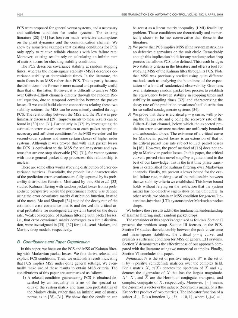
Fig. 1. Estimation over an erasure channel.

if ω ∈ A, otherwise 1A(ω) = 0. For random variables, σ(·) isthe σ-algebra generated by the variables.

II. KALMAN FILTERING WITH MARKOVIAN PACKET LOSSES

Consider an LTI system

xk+1 = Axk + wk (1a)

yk = Cxk + vk (1b)

where A ∈ Rn×n is the system matrix and C ∈ Rm×n isthe observation matrix, xk ∈ Rn is the process state vec-tor and yk ∈ Rm is the observation vector, wk ∈ Rn andvk ∈ Rm are zero-mean Gaussian random vectors with auto-covariance E[wkwj ′] = δkjQ (Q ≥ 0), E[vkvj ′] = δkjR (R >0), E[wkvj ′] = 0 ∀j, k. Here, δkj is the Kronecker delta func-tion with δkj = 1 if k = j and δkj = 0 otherwise. The initialstate x0 is a zero-mean Gaussian random vector that is uncor-related with wk and vk and has covariance Σ0 ≥ 0. We assumethat (C,A) is detectable and (A,Q1/2) is stabilizable. By apply-ing a similarity transformation, the unstable and stable modesof the considered LTI system can be decoupled. An open-loopprediction of the stable mode always has a bounded estimationerror covariance, therefore, this mode does not play any key rolein the stability issues considered in this paper. Without loss ofgenerality, we assume that (A1) All the eigenvalues of A havemagnitudes no less than 1. Certainly A is nonsingular.

We consider an estimation scheme illustrated in Fig. 1, wherethe raw measurements of the sensor {yk}k∈N are transmitted tothe estimator via an erasure communication channel over whichpackets may be dropped randomly. Denote by γk ∈ {0, 1} thearrival of yk at time k: yk arrives errorfree at the estimator ifγk = 1; otherwise γk = 0. Whether γk takes value 0 or 1 isassumed to be known by the receiver at time k. Define Fk asthe filtration generated by all the measurements received by theestimator up to time k, i.e., Fk � σ (γtyt , γt ; 1 ≤ t ≤ k) andF = σ (∪∞

k=1Fk ). We will use a triple (Ω,F ,P ) to denote theprobability space capturing all the randomness in the model.

To describe the temporal correlation of realistic communica-tion channels, we assume the Gilbert–Elliott channel [23], [24],where the packet loss process is a time-homogeneous two-stateMarkov chain. To be precise, {γk}k∈N is the state of the Markovchain with initial condition, without loss of generality, γ1 = 1.The transition probability matrix for the Gilbert–Elliott channelis given by

P =[

1 − q qp 1 − p

](2)

where p � P (γk+1 = 0|γk = 1) is called the failure rate, andq � P (γk+1 = 1|γk = 0) the recovery rate. Assume that (A2)The failure and recovery rates satisfy p, q ∈ (0, 1).

The estimator computes xk |k , the minimum mean-squarederror estimate, and xk+1|k , the one-step prediction, accord-ing to xk |k = E[xk |Fk ] and xk+1|k = E[xk+1 |Fk ]. Let Pk |kand Pk+1|k be the corresponding estimation and prediction er-ror covariance matrices, i.e., Pk |k = E[(xk − xk |k )(·)′|Fk ] andPk+1|k = E[(xk+1 − xk+1|k )(·)′|Fk ]. They can be computedrecursively via a modified Kalman filter [16]. The recursions forxk |k and xk+1|k are omitted here. To study the Kalman filteringsystem’s stability, we focus on the prediction error covariancematrix Pk+1|k , which is recursively computed as

Pk+1|k = APk |k−1A′ +Q

−γkAPk |k−1C′(CPk |k−1C

′ +R)−1CPk |k−1A′.

It can be seen that Pk+1|k inherits the randomness of {γt}1≤t≤k .We focus on characterizing the impact of {γk}k∈N on Pk+1|k .To simplify notations in the sequel, let Pk+1 � Pk+1|k , anddefine the functions h, g, hk , and gk : Sn

+ → Sn+ as follows

h(X) � AXA′ +Q (3)

g(X) � AXA′ +Q−AXC ′(CXC ′ +R)−1CXA′

hk (X) � h ◦ h ◦ · · · ◦ h︸︷︷︸ktimes

(X) and gk (X) � g ◦ g ◦ · · · ◦ g︸︷︷︸ktimes

(X)

(4)

where ◦ denotes the function composition. The following sta-bility notion is standard.

Definition 1: The Kalman filtering system with packet lossesis mean-square stable if supk∈N E‖Pk‖ <∞.

Define

τ1 � min{k : k ∈ N, γk = 0}β1 � min{k : k > τ1 , γk = 1}

...

τj � min{k : k > βj−1 , γk = 0}βj � min{k : k > τj , γk = 1}. (5)

It is straightforward to verify that {τj}j∈N and {βj}j∈N aretwo sequences of stopping times because both {τj ≤ k} and{βj ≤ k} are Fk−measurable; see [38] for details. Due to thestrong Markov property and the ergodic property of the Markovchain defined by (2), the sequences {τj}j∈N and {βj}j∈N havefinite values P -almost surely. Then, we can define the so-journ times at the state 1 and state 0, respectively, by τ ∗j andβ∗j ∀j ∈ N as

τ ∗j � τj − βj−1 and β∗j � βj − τj

where β0 = 1 by convention. A result given by [29, Lemma 2]demonstrates that {τ ∗k}j∈N and {β∗

k}j∈N are mutually indepen-dent and have geometric distribution. Let us denote the predic-tion error covariance matrix at the stopping time βj by Pβj and


Fig. 2. Road map of this work.

call it the peak covariance1 at βj . We introduce the notion ofPCS [29] as follows:

Definition 2: The Kalman filtering system with packet lossesis said to be peak-covariance stable if supj∈N E‖Pβj ‖ <∞.

Remark 1: In [32], the authors defined stability in stoppingtimes as the stability of Pk at packet reception times. Note that{βj}j∈N , at which the peak covariance is defined, can also betreated as the stopping times defined on packet reception times.Clearly, in scalar systems, the covariance is at maximum whenthe channel just recovers from failed transmissions; therefore,peak covariance sequence gives an upper envelop of covariancematrices at packet reception times. For higher order systems,the relation between them is still unclear.

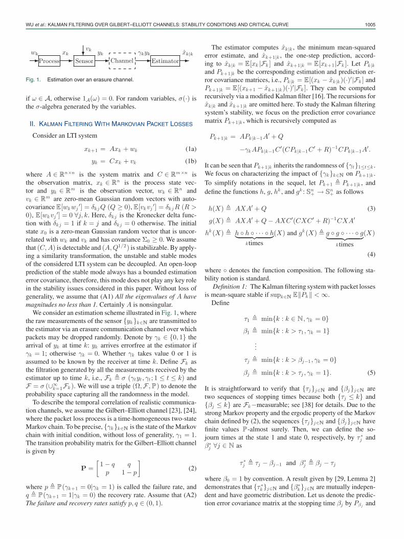
The results of this paper are organized as follows (cf., Fig. 2).First of all, we present a relaxed condition for PCS (Theorem 1).Then, we establish a result indicating that for general packet dropprocesses PCS implies MSS under mild conditions (Theorem 2).We continue to show that MSS inherits a sharp phase transitionreflected by a critical p− q curve (Theorem 3). We finally man-age to combine all these results and conclude an MSS conditionfor general LTI systems (Theorem 4).

III. PEAK-COVARIANCE STABILITY

In this section, we study the PCS [29] of the Kalman filter.(9) shown at the bottom of this page.

We introduce the observability index of the pair (C,A).

1The definition of peak covariance was first introduced in [29], where theterm “peak” was attributed to the fact that for an unstable scalar system Pkmonotonically increases to reach a local maximum at time βj . This maximumproperty does not necessarily hold for the multidimensional case.

Definition 3: The observability index Io is defined as thesmallest integer such that [C ′, A′C ′, . . . , (AIo−1)′C ′]′ has rankn. If Io = 1, the system (C,A) is called one-step observable.

We also introduce the operator LK : Sn+ → Sn

+ defined as

LK (X) = p

Io−1∑i=1

(1−p)i−1(Ai+K(i)C(i))∗ΦX (Ai +K(i)C(i))

(6)where ΦX is the positive definite solution of the Lyapunov equa-tion (1 − q)A′ΦXA+ qA′XA = ΦX with |λA |2(1 − q) < 1,and K = [K(1) , . . . ,K(Io−1) ] with each matrix K(i) havingcompatible dimensions. It can be easily shown that LK (X)is linear and nondecreasing in the positive semidefinite cone.

We have the following result.Theorem 1: Suppose |λA |2(1 − q) < 1. If any of the follow-

ing conditions hold.i) ∃K � [K(1) , . . . ,K(Io−1) ], where K(i)s are matrices

with compatible dimensions, such that |λH (K ) | < 1,where

H(K) = qp[(A⊗A)−1 − (1 − q)I

]−1

·Io−1∑i=1

(Ai +K(i)C(i))

⊗ (Ai +K(i)C(i))(1 − p)i−1 . (7)

ii) There exists K � [K(1) , . . . ,K(Io−1) ] with each ma-trix K(i) having compatible dimensions such thatlimk→∞ LkK (X) = 0 for any X ∈ Sn

+ .iii) There exist K � [K(1) , . . . ,K(Io−1) ] with each matrix

K(i) having compatible dimensions andP > 0 such thatLK (P ) < P .

iv) There exist F1 , . . . , FIo−1 , X > 0, Y > 0 such that⎡⎣ Y

√1 − qA′Y

√qA′X√

1 − qY A Y 0√qXA 0 X

⎤⎦ ≥ 0 (8)

and Ψ > 0 where Ψ is given in (9).Then, supj≥1 E‖Pβj ‖ <∞, i.e., the Kalman filtering system

is peak-covariance stable.The proof of Theorem 1 is given in Appendix B. For con-

dition (i) of Theorem 1, a quite heavy computational overheadmay be incurred in searching for a satisfactory K. Condition(iv), as an LMI interpretation of condition (i), makes it possi-ble to check the sufficient condition for PCS through an LMIfeasibility criterion.

Remark 2: Theorem 1 establishes a direct connection be-tween λH (K ) , p, q, the most essential aspects of the system

Ψ �

⎡⎢⎢⎢⎣

X√p(A′Y + C ′F1) · · · √

p(1 − p)Io−2((AIo−1)′Y + (C(i))′FIo−1

)√p(Y A+ F ∗

1C) Y · · · 0...

.... . .

...√p(1 − p)Io−2

(Y AIo−1 + F ∗

Io−1C(i)

)0 · · · Y

⎤⎥⎥⎥⎦

(9)


dynamic and channel characteristics on the one hand, and PCSon the other hand. These results cover the ones in [28], [29],and [31], as is evident using the subadditivity property of matrixnorm, and the fact that the spectral radius is the infimum of allpossible matrix norms. To see this, one should notice that

|λH (k) |

≤ qp∥∥∥[(A⊗A)−1 − (1 − q)I

]−1∥∥∥Io−1∑i=1

(1 − p)i−1∥∥∥(Ai +K(i)C(i)) ⊗ (Ai +K(i)C(i))

∥∥∥

≤ qp

∞∑i=1

(1 − q)i−1‖Ai ⊗Ai‖

Io−1∑i=1

(1 − p)i−1∥∥∥(Ai +K(i)C(i)) ⊗ (Ai +K(i)C(i))

∥∥∥

= q

∞∑i=1

(1 − q)i−1‖Ai‖2p

Io−1∑i=1

(1 − p)i−1‖Ai +K(i)C(i)‖2

in which the first inequality follows from |λH (K ) | ≤ ‖H(K)‖and the submultiplicative property of matrix norms, andthe last equality holds because, for a matrix X , ‖Xi ⊗Xi‖ =

√λ

(Xi(X ′)i )⊗(X i (X ∗)i )

= λX i (X ∗)i = ‖Xi‖2 . Compar-

ison with the related results in the literature is also demonstratedby Example I in Section V.

In addition, in [28], [29], and [31], the criteria for PCS aredifficult to check since some constants related to the operatorg are hard to explicitly compute. A thorough numerical searchmay be computationally demanding. In contrast, the stabilitycheck of Theorem 1 uses an LMI feasibility problem, which canoften be efficiently solved.

In the following proposition, we present another condition forPCS, which is, despite being conservative, easy to check. Thenew condition is obtained by making all K(i)s in Theorem 1take the value zero.

Proposition 1: If the following condition is satisfied

pq|λA |2Io−1∑i=1

|λA |2i(1 − p)i−1 < 1 − |λA |2(1 − q), (10)

then the Kalman filtering system is peak-covariance stable.Proof: The proof requires the following lemma.Lemma 1 ([39, Th. 1.1.6]): Let p(·) be a given polynomial.

If λ is an eigenvalue of a matrix A, then, p(λ) is an eigenvalueof the matrix p(A).

Define a sequence of polynomials of the matrix A⊗A as{pn (A⊗A)}n∈N , where

pn (A⊗A) =n∑i=1

(A⊗A)i(1 − q)i−1q

×Io−1∑j=1

(A⊗A)j (1 − p)j−1p.

In light of Lemma 1, the spectrum of pn (A⊗A) isgiven by σ (pn (A⊗A)) = {pn (λiλj ) : λi , λj ∈ σ(A)}. SinceA is a real matrix, its complex eigenvalues, if any, al-ways occur in conjugate pairs. Therefore, |λA |2 mustbe an eigenvalue of A⊗A, and the spectral radius ofpn (A⊗A) can be computed as |λpn (A⊗A) | =

∑ni=1 |λA |2i(1 −

q)i−1q∑Io−1

j=1 |λA |2j (1 − p)j−1p. It is evident that the sequence{|λpn (A⊗A) |}n∈N is monotonically increasing. When |λA |2(1 −q) < 1, we have

limn→∞ pn (A⊗A) = H(0) (11)

and

limn→∞ |λpn (A⊗A) | =

q|λA |21 − |λA |2(1 − q)

Io−1∑j=1

|λA |2j (1 − p)j−1p.

(12)As |λX | is continuous with respect to X , (11) and (12) alto-

gether lead to |λH (0) | = q |λA |21−|λA |2 (1−q)

∑Io−1j=1 |λA |2j (1 − p)j−1p.

Letting K(i) = 0 ∀1 ≤ i ≤ Io − 1, the condition provided inTheorem 1 becomes: (i) |λA |2(1 − q) < 1, and (ii) |λH (0) | < 1.Since the left side of (10) is positive, it imposes the positivity of1 − |λA |2(1 − q), whereby the conclusion follows. �

Although computationally friendly, Proposition 1 only pro-vides a comparably rough criterion. It can be expected that,given the ability of searching for K(i)s on the positive semidef-inite cone, Theorem 1 is less conservative than Proposition 1;this is demonstrated by Example I in Section V.

Remark 3: The left side of (10) is strictly positive whenIo ≥ 2, while it vanishes when Io = 1. In the latter case, plus thenecessity as shown in [30], |λA |2(1 − q) < 1 thereby becomesa necessary and sufficient condition for PCS. This observationis consistent with the conclusion of [31, Corollary 2].

Remark 4: Proposition 1 covers the result of [30, Th. 3.1].To see this, notice that

q|λA |21 − |λA |2(1 − q)

Io−1∑j=1

|λA |2j (1 − p)j−1p

=∞∑i=1

|λA |2i(1 − q)i−1q

Io−1∑j=1

|ΛA |2j (1 − p)j−1p

≤∞∑i=1

‖Ai‖2(1 − q)i−1q

Io−1∑j=1

‖Aj‖2(1 − p)j−1p,

which implies the less conservativity of [30, Th. 3.1].

IV. MEAN-SQUARE STABILITY

In this section, we will discuss MSS of Kalman filtering withMarkovian packet losses.

A. From PCS to MSS

Note that the PCS characterizes the filtering system atstopping times defined by (5), whereas MSS characterizes theproperty of stability at all sampling times. In the literature,the relationship between the two stability notations is still an


open problem. In this section, we aim to establish a connectionbetween PCS and MSS. First, we need the following definitionfor the defective eigenvalues of a matrix.

Definition 4: For λ ∈ σ(A) where A is a matrix, if the alge-braic multiplicity and the geometric multiplicity of λ are equal,then λ is called a semisimple eigenvalue ofA. If λ is not semisim-ple, λ is called a defective eigenvalue of A.

We are now able to present the following theorem indicatingthat as long as A has no defective eigenvalues on the unit cir-cle, i.e., the corresponding Jordan block is 1 × 1, PCS alwaysimplies MSS. In fact, we are going to prove this connectionfor general random packet drop processes {γk}k∈N , instead oflimiting to the Gilbert–Elliott model.

Theorem 2: Let {γk}k∈N be a random process over an un-derlying probability space (S ,S, μ) with each γk taking itsvalue in {0, 1}. Suppose {βj}j∈N take finite values μ−almostsurely, and thatA has no defective eigenvalues on the unit circle.Then, the PCS of the Kalman filter always implies MSS, i.e.,supk∈N E‖Pk‖ <∞ whenever supj∈N E‖Pβj ‖ <∞.

Note that {βj}j∈N can be defined over any random packet lossprocesses, therefore, the PCS with packet losses that the filteringsystem is undergoing remains in accord with Definition 2.

Theorem 2 bridges the two stability notions of Kalman fil-tering with random packet losses in the literature. Particu-larly, this connection covers most of the existing models forpacket losses, e.g., i.i.d. model [16], bounded Markovian [40],Gilbert–Elliott [28], and finite-state channel [25], [26]. Althoughsupk∈N E‖Pk‖ and supj∈N E‖Pβj ‖ are not equal in general,this connection is built upon a critical understanding that, nomatter to which interarrival interval between two successive βj sthe time k belongs, ‖Pk‖ is uniformly bounded from above byan affine function of the norm of the peak covariances at thestarting and ending points thereof. This point holds regardlessof the model of packet loss process. The proof of Theorem 2was given in Appendix C.

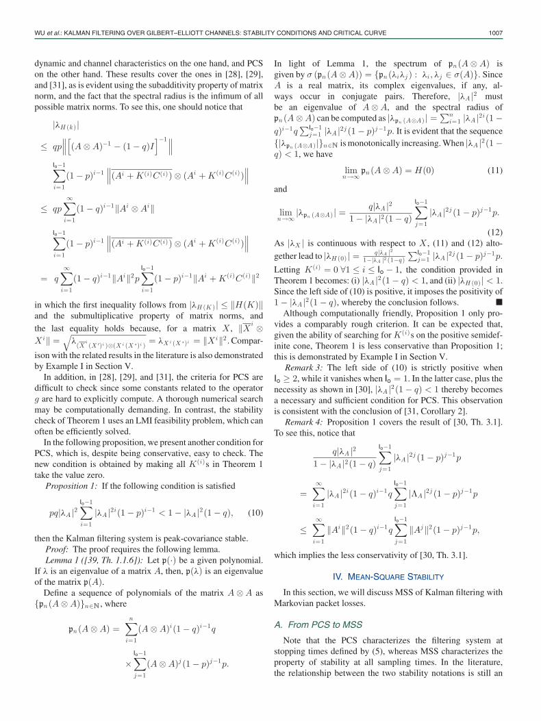
We also remark that there is difficulty in relaxing the assump-tion that A has no defective eigenvalues on the unit circle inTheorem 2. This is due to the fact that As defective eigenvalueson the unit circle will influence both the PCS and MSS in anontrivial manner (see Fig. 3).

Remark 5: In [29], for a scalar model with i.i.d. packetlosses, it has been shown that the PCS is equivalent to MSS,whereas for a vector system even with i.i.d. packet losses, therelationship between the two is unclear. In [31], the equivalencebetween the two stability notions was established for systemsthat are one-step observable, again for the i.i.d. case. Theorem 2now fills the gap for a large class of vector systems under generalrandom packet drops.

B. The Critical p− q Curve

In this section, we first show that for a fixed q in the Gilbert–Elliott channel, there exists a critical failure rate pc , such that ifand only if the failure rate is below pc , the Kalman filtering ismean-square stable. This conclusion is relatively independentof previous results, and the proof relies on a coupling argumentand can be found in Appendix D.

Fig. 3. Relationships between the PCS and MSS over the space ofthe filtering systems under consideration. Theorem 2 indicates that theintersection of the two sets, PCS and NoDEUC, is contained in the setMSS.

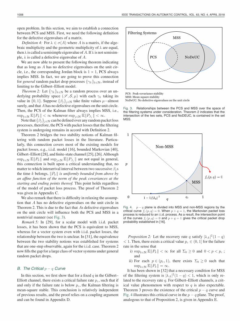
Fig. 4. p − q plane is divided into MSS and non-MSS regions by thecritical curve fc (p, q) = 0. When p + q = 1, the Markovian packet lossprocess is reduced to an i.i.d. process. As a result, the intersection pointof the curves fc (p, q) = 0 and p + q = 1 gives the critical packet dropprobability established in [16].

Proposition 2: Let the recovery rate q satisfy |λA |2(1 − q)< 1. Then, there exists a critical value pc ∈ (0, 1] for the failurerate in the sense that

i) supk∈N E‖Pk‖ <∞ for all Σ0 ≥ 0 and 0 < p < pc ;and

ii) For each p ∈ (pc , 1), there exists Σ0 ≥ 0 such thatsupk∈N E‖Pk‖ = ∞.

It has been shown in [32] that a necessary condition for MSSof the filtering system is |λA |2(1 − q) < 1, which is only re-lated to the recovery rate q. For Gilbert–Elliott channels, a crit-ical value phenomenon with respect to q is also expectable.Theorem 3 proves the existence of the critical p− q curve andFig. 4 illustrates this critical curve in the p− q plane. The proof,analogous to that of Proposition 2, is given in Appendix E.


Theorem 3: There exists a critical curve defined byfc(p, q) = 0, which reads two nondecreasing functions p =pc(q) and q = qc(p) with qc(·) = p−1

c (·), dividing (0, 1)2 intotwo disjoint regions such that

i) If (p, q) ∈ {fc(p, q) > 0

}, then, supk∈N E‖Pk‖ <∞

for all Σ0 ≥ 0;ii) If (p, q) ∈ {

fc(p, q) < 0}

, then, there exists Σ0 ≥ 0 un-der which supk∈N E‖Pk‖ = ∞.

Remark 6: If the packet loss process is an i.i.d. process,where p+ q = 1 in the transition probability matrix definedin (2), Proposition 2 and Theorem 3 recover the result of[16, Th. 2]. It is worth pointing out that whether MSS holdsor not exactly on the curve fc(p, q) = 0 is beyond the reach ofthe current analysis (even for the i.i.d. case with p+ q = 1):such an understanding relies on the compactness of the stabilityor nonstability regions.

C. MSS Conditions

We can now make use of the PCS conditions we obtainedin the last section, and the connection between PCS and MSSindicated in Theorem 2, to establish MSS conditions for the con-sidered Kalman filter. It turns out that the assumption requiringno defective eigenvalues on the unit circle can be relaxed by anapproximation method. We present the following result.

Theorem 4: Let the recovery rate q satisfy |λA |2(1 − q) < 1.Then, there holds p ≤ pc , where

p � sup{p : ∃(K,P ) s.t. LK (P ) < P,P > 0

}(13)

i.e., for all Σ0 ≥ 0 and 0 < p < p, the Kalman filtering systemis mean-square stable.

The proof of Theorem 4 is given in Appendix F.Remark 7: For second-order systems and certain classes of

higher order systems, such as nondegenerate systems, necessaryand sufficient conditions for MSS have been derived in [32]and [34]. However, these results rely on a particular systemstructure and fail to apply to general LTI systems. Theorem 4gives a stability criterion for general LTI systems.

V. NUMERICAL EXAMPLES

In this section, we present two numerical examples to demon-strate the theoretical results we established in Sections IIIand IV.

A. Example I: A Second-order System

To compare with the works in [28]–[30], we will examine thesame vector example considered therein. The parameters arespecified as follows

A =[

1.3 0.30 1.2

], C = [1, 1]

Q = I2×2 and R = 1. As illustrated in [29], it is easily checkedthat Io = 2 and the spectrum ofA is σ(A) = {1.2, 1.3}, and thatλA = 1.3.

Note that |λA |2(1 − q) < 1 is a necessary condition for MSS.We take q = 0.65 as was done in [29]. As for the failure rate

Fig. 5. Sample path of ‖Pk ‖ with p = 0.99, q = 0.65 in Example I.

Fig. 6. Sample path of ‖Pk ‖ with p = 0.45, q = 0.5 in Example II.

p, [29] concludes that p < 0.04 guarantees PCS; while Proposi-tion 1 requires p < 1−|λA |2 (1−q)

|λA |4 q , which generates a less conser-vative condition p < 0.22. Similarly, the example in [30] allowsp = 0.1191 at most. We also note that it is rather convenient tocheck the condition in Proposition 1 even with manual calcula-tion; in contrast, to check the conditions in [29] and [30] involvesa considerable amount of numerical calculation. Additionally,we use the criterion established in Theorem 1 to check for thePCS. We obtain that when p = 1, the LMI in (ii) of Theorem 1is still feasible.2 Fig. 5 illustrates sample paths of ‖Pk‖ with(p, q) = (0.99, 0.65), which shows that even a high value of pmay not affect the PCS in this example.

B. Example II: A Third-order System

To compare the work in Section IV with the result of[32]and [34], we will use the following example, where the param-eters are given by

A =

⎡⎣1.2 0 0

0 1.2 00 0 −1.2

⎤⎦ , C =

[1 0 10 1 1

](14)

Q = I3×3 and R = I2×2 .1) Mean-Square Stability: The system described in (14)

is observable and degenerate [22]. Therefore, the MSS condi-tions presented in [32] and [34] for nondegenerate systems arenot applicable in this example. In contrast, our Theorem 4 pro-vides a universal criterion for MSS. Fixing q = 0.5, we canconclude from Theorem 4 that if p ≤ 0.465 the Kalman filteris mean-square stable. Fig. 6 illustrates a stable sample pathof ‖Pk‖ with (p, q) = (0.45, 0.5). On the other hand, when(p, q) = (0.99, 0.5) the expected prediction error covariancematrices diverge (as illustrated in Fig. 7). One can check that

2To satisfy the assumption (A2), we need to configure p = 1 − ε for anarbitrary small positive ε.


Fig. 7. Divergence of E‖Pk ‖ with p = 0.99, q = 0.5 in Example II.

Fig. 8. Blue-colored crosses represent (p, q) points where the Kalmanfilter is mean-square stable; the gray dots represent (p, q) points atwhich the Kalman filter is mean-square unstable. Clearly a critical curveemerges.

when (p, q) = (0.99, 0.5) the criterion in Theorem 4 is violated.This verifies the contrapositive of Theorem 4.

2) Critical Curve: We now illustrate the result ofTheorem 3 by Monte Carlo simulations. We quantize the p− qplane with a step size 0.025 along each axis. For each discretized(p, q) value, we run Monte Carlo simulations for N = 100 000repeated rounds, and each sample goes through 70 time steps.Noticing that without packet loss, the norm of the steady esti-mation error covariance is around 3.7, we use

Papp =1N

N∑i=1

‖Pk (ωi)‖

with k = 70 as the empirical approximation of E[Pk ] and seta criterion Papp ≤ 100 for MSS. Clearly the p− q plane con-sists of a stable and another unstable regions, separated by anemerging critical curve (see Fig. 8).

VI. CONCLUSION

We have investigated the stability of Kalman filtering overGilbert–Elliott channels. Random packet drops follow a time-homogeneous two-state Markov chain where the two statesindicate successful or failed packet transmissions. We estab-lished a relaxed condition guaranteeing PCS described by aninequality in terms of the spectral radius of the system ma-trix and transition probabilities of the Markov chain, and thenshowed that the condition can be reduced to an LMI feasibilityproblem. It was proved that PCS implies MSS if the systemmatrix has no defective eigenvalues on the unit circle. This

connection holds for general random packet drop processes. Wealso proved that there exists a critical region in the p− q planesuch that if and only if the pair of recovery and failure ratesfalls into that region the expected prediction error covariancematrices are uniformly bounded. By fixing the recovery rate, alower bound for the critical failure rate was obtained makinguse of the relationship between two stability criteria for generalLTI systems. Numerical examples demonstrated significant im-provement on the effectiveness of our approach compared withthe existing literature.

APPENDIX AAUXILIARY LEMMAS

In this section, we collect some lemmas that are used in theproofs of our main results.

Lemma 2 (Lemma A.1 in [33]): For any matrices X ≥ Y≥ 0, the following inequalities hold

h(X) ≥ h(Y ) (15)

g(X) ≥ g(Y ) (16)

h(X) ≥ g(X) (17)

where the operators h and g are defined in (3) and (4),respectively.

Lemma 3: Consider the operator

φi(K(i) , P ) � (Ai +K(i)C(i))X(·)∗

+[A(i) K(i) ][Q(i) Q(i)(D(i))′

∗ D(i)(Q(i))(D(i))′ +R(i)

][A(i) K(i) ]∗

for all i ∈ N, whereC(i) = [C ′, A′C ′, . . . , (A′)i−1C ′]′,A(i) =[Ai−1 , . . . , A, I], D(i) = 0 for i = 1 otherwise

D(i) =

⎡⎢⎢⎢⎣

0 0 · · · 0C 0 · · · 0...

.... . .

...CAi−2 CAi−3 · · · 0

⎤⎥⎥⎥⎦ ,

Q(i) = diag(Q, . . . , Q︸︷︷︸i

), R(i) = diag(R, . . . , R︸︷︷︸i

), and K(i) are

of compatible dimensions. For any X ≥ 0 and K(i) , it alwaysholds that gi(X) = minK ( i ) φi(K(i) ,X) ≤ φi(K(i) ,X).

Proof: The result is readily established when setting B = Iin [40, Lemmas 2 and 3]. For i = 1, The result is well known asin [16, Lemma 1].

Lemma 4 ([41]): For any A ∈ Cn×n , ε > 0 and k ∈ N, it

holds that ‖Ak‖ ≤ √n(1 + 2/ε)n−1

(|λA | + ε‖A‖

)k.

Lemma 5 (Lemma 2 in [42]): For any G ∈ Cn×n , there ex-ist Gi ∈ Sn

+ , i = 1, 2, 3, 4 such that G = (G1 −G2) + (G3 −G4)i, where i =

√−1.

APPENDIX BPROOF OF THEOREM 1

The proof is lengthy and is divided into two parts. In the firstpart, we will show that condition i) is a sufficient condition for


PCS. In the second part, we will show the equivalence betweenconditions i)–iv). The proof relies on the following two lemmas.

Lemma 6 ( [29, Lemma 5]): Assume that (C,A) is observ-able and (A,Q1/2) is controllable. Define

Sn0 � {P : 0 ≤ P ≤ AP0A

′ +Q, for some P0 ≥ 0}.

Then, there exists a constant L > 0 such thati) for any X ∈ Sn

0 , gk (X) ≤ LI for all k ≥ Io; andii) for any X ∈ Sn

+ , gk+1(X) ≤ LI for all k ≥ Iowhere the operator g is defined in (4).Lemma 7: For q ∈ (0, 1) andA ∈ Rn×n , the series of matri-

ces∑∞

i=1(A⊗A)i(1 − q)i−1q and∑∞

i=1∑i−1

j=0(A⊗A)j (1 −q)i−1q converge if and only if |λA |2(1 − q) < 1.

Proof: First observe that∑∞

i=1∑i−1

j=0(A⊗A)j (1 −q)i−1q =

∑∞i=0(A⊗A)i(1 − q)i . The geometric series

generated by (A⊗A)(1 − q) converges if and only if|λA⊗A |(1 − q) < 1. Therefore, the conclusion follows from thefact that |λA⊗A | = max{|λiλj | : λi , λj ∈ σ(A)} = |λA |2 . �

Now, fix j ≥ 1. First note that, for any k ∈ [τj+1 , βj+1 − 1],γk = 0. Hence, we have

Pβj + 1 =∞∑i=1

1{β ∗j + 1 =i}hi(Pτj + 1 )

�∞∑i=1

1{β ∗j + 1 =i}AiPτj + 1 (A

i)′ +∞∑i=1

1{β ∗j + 1 =i}Vi (18)

where Vi �∑i−1

l=0 AlQ(Al)′. Now, let us consider the inter-

val [βj , τj+1 − 1] over which τ ∗j+1 packets are successfully re-ceived. We will analyze the relationship between Pτj + 1 and Pβjin two separate cases, which are τ ∗j+1 ≤ Io − 1 and τ ∗j+1 ≥ Io.Computation yields the following result

Pτj + 1 =Io−1∑i=1

1{τ ∗j + 1 =i}gi(Pβj ) +

∞∑l= Io

1{τ ∗j + 1 = l}gl(Pβj )

≤Io−1∑i=1

1{τ ∗j + 1 =i}φi(K(i) , Pβj ) + LI

∞∑l= Io

1{τ ∗j + 1 = l}

=Io−1∑i=1

1{τ ∗j + 1 =i}(Ai +K(i)C(i))Pβj (A

i +K(i)C(i))∗

+ LI∞∑j= Io

1{τ ∗j + 1 = l} +

Io−1∑i=1

1{τ ∗j + 1 =i}[Ai K(i)]Ji [Ai K(i)]∗

� (Ai +K(i)C(i))Pβj (Ai +K(i)C(i))∗ + U (19)

where Ji �[

Q(i) Q(i)(D(i))′

D(i)(Q(i)) D(i)(Q(i))(D(i))′ +R(i)

]and

U � LI∞∑j= Io

1{τ ∗j + 1 = l} +

Io−1∑i=1

1{τ ∗j + 1 =i}[Ai K(i) ]Ji [Ai K(i) ]∗

is bounded. The first inequality is from Lemmas 3 and 6. Bysubstituting (19) into (18), it yields

Pβj + 1 ≤W +∞∑i=1

1{β ∗j + 1 =i}Ai

×[

Io−1∑l=1

1{τ ∗j + 1 = l}(·)Pβj (Al +K(l)C(l))∗

](Ai)′ (20)

where W �∑∞

i=1 1{β ∗j + 1 =i}AiU(Ai)′ +

∑∞i=1 1{β ∗

j + 1 =i}Vi .To facilitate discussion, we force Pβj + 1 in (20) to take themaximum. For other cases in (20), the subsequent conclusionstill holds as it renders an upper envelop of {Pβj }j∈N byimposing (20) to take equality.

We introduce the vectorization operator. Let X =[x1 x2 · · · xn ] ∈ Cm×n where xi ∈ Cm . Then, we definevec(X) � [x′1 , x

′2 , . . . , x

′n ]′ ∈ Cmn . Notice that vec(AXB) =

(B′ ⊗A)vec(X). For Kronecker product, we have (A1A2) ⊗(B1B2) = (A1 ⊗B1) (A2 ⊗B2). Take expectations and vec-torization operators over both sides of (20). From [29,Lemma 2], we obtain

E[vec(Pβj + 1 )] = E[vec(W )]

+∞∑i=1

(A⊗A)i(1 − q)i−1q

·Io−1∑l=1

(Al +K(l)C(l)) ⊗ (·)p(1 − p)l−1 E[vec(Pβj )].

(21)

In the above-mentioned equation E[vec(W )] can be written as

E[vec(W )]=∞∑i=1

(A⊗A)i(1 − q)i−1q vec(U)

+∞∑i=1

i−1∑l=0

(A⊗A)l(1 − q)i−1q vec(Q). (22)

In Lemma 7, we show that both of the two terms in (22) convergeif |λA |2(1 − q) < 1.

For j = 1, following the similar argument as abovemen-tioned, we have

E‖Pβ1 ‖ ≤ E‖Pτ1 ‖∞∑i=1

‖Ai‖2(1 − q)i−1q

+∥∥∥

∞∑i=1

(1 − q)i−1qVi

∥∥∥where Vis are defined in (18). Moreover, by Lemma 6 and (17),it holds that

E‖Pτ1 ‖ ≤ ‖LI‖ +Io∑i=1

‖gi(Σ0)‖(1 − p)i−1p

≤ ‖LI‖ + ‖Σ0‖Io∑i=1

‖Ai‖2(1 − p)i−1p+ ‖VIo‖


showing that E‖Pτ1 ‖ is bounded. To sum up, E‖Pβ1 ‖ isbounded if |λA |2(1 − q) < 1. By applying the Cauchy–Schwarzinequality to the inner product of random variables, the bound-ness of E‖Pβ1 ‖ implies the boundness of each element ofE[Pβ1 ]. So is E[vec(Pβ1 )] if |λA |2(1 − q) < 1.

We have shown that E[vec(Pβj )] for j ∈ N evolves fol-lowing (21), and that E[vec(W )] in (21) and E[vec(Pβ1 )] arebounded if |λA |2(1 − q) < 1. We conclude that if |λA |2(1 −q) < 1 and there exists an K � [K(1) , . . . ,K(Io−1) ] such that|λH (K ) | defined in (7) is less than 1, then the spectral radius of

∞∑i=1

(A⊗A)i(1 − q)i−1q

Io−1∑l=1

(Al +K(l)C(l)) ⊗ (·)(1 − p)l−1p

is less than 1, all the above-mentioned observations lead tosupj≥1 E[veci(Pβj )] <∞ ∀1 ≤ i ≤ n2 , where veci(X) repre-sents the ith element of vec(X). In addition, there holds

E‖Pβj ‖ ≤ E[tr(Pβj )

]= [e′1 , . . . , e

′n ] E[vec(Pβj )]

where ei denotes the vector with 1 in the ith coordinate and 0selsewhere, so the desired result follows.

ii) ⇒ i). It suffices to show |λH ∗(K ) | < 1. The hypothesismeans that for any X ∈ Sn

+

limk→∞

(H∗(K))k vec(X) = 0. (23)

In light of Lemma 5, for any G ∈ Cn×n there ex-ist G1 , G2 , G3 , G4 ∈ Sn

+ such that G = (G1 −G2) + (G3 −G4)i. It can been seen from (23) that

limk→∞

(H∗(K))k vec(G)

= limk→∞

(H∗(K))k (vec(G1) − vec(G2))

+ limk→∞

(H∗(K))k (vec(G3) − vec(G4)) i = 0

which implies i).i) ⇒ iii). Since |λH ∗(K ) | < 1 by the hypothesis in (i), (I −

H∗(K))−1 exist and it equals to∑∞

i=0 (H∗(K))i . Due to thenonsingularity of (I −H∗(K))−1 and the one-to-one corre-spondence of vectorization operator, for any positive definitematrix V ∈ Cn×n , there exists a unique matrix P ∈ Cn×n suchthat

vec(V ) = (I −H∗(K)) vec(P ). (24)

The property of Kronecker product gives vec(V ) =vec (P − LK (P )) . Since, vectorization is one-to-one corre-spondence, we then have V = P − LK (P ) > 0. It still remainsto show P > 0. It follows from (25) that

vec(P ) = (I −H∗(K))−1 vec(V )

=∞∑i=0

(H∗(K))i vec(V )

= vec

( ∞∑i=0

LiK (V )

)(25)

which yields P =∑∞

i=0 LiK (V ) > 0.

iii) ⇒ ii). If there exist K = [K(1) , . . . ,K(Io−1) ] with eachmatrix K(i) having compatible dimensions and P > 0 suchthat LK (P ) < P , then there must exist a μ ∈ (0, 1) satisfyingLK (P ) < μP . Choose c > 0 such that X ≤ cP . Then, due tothe linearity and nondecreasing properties of LK (X) with re-spect to X on the positive semidefinite cone, for k ∈ N

LkK (X) ≤ LkK (cP ) = cLkK (P ) < cLk−1K (μP ) < · · · < cμkP

which leads to limk→∞ LkK (X) = 0.iii) ⇒ iv). The proof is similar to the proof of b) ⇒ c) in [16,

Th. 5] and is omitted here.iv) ⇒ iii). Note that, by the Schur complement lemma and

X,Y > 0, (8) holds if and only if

Y ≥ (1 − q)A′Y A+ qA′XA. (26)

Similarly, (9) holds if and only if

p

Io−1∑i=1

(1 − p)i−1(Ai +K(i)C(i))∗Y (Ai +K(i)C(i)) < X

(27)where K(i) = Y −1F ∗

i , i = 1, . . . , Io − 1. Applying the in-equality of (26) for k times, it results in

Y ≥ (1 − q)k (A′)kY Ak + q

k∑j=1

(1 − q)j−1(A′)jXAj .

As Y is bounded, taking limitation on the right sides, it yields

Y ≥ q∞∑j=1

(1 − q)j−1(A′)jXAj . (28)

Combining (27) and (28), we obtain LK (X) < X .

APPENDIX CPROOF OF THEOREM 2

To prove this theorem, we need some preliminary lemmas.Lemma 8: Suppose that there exist constants d1 ,

d0 ≥ 0 such that, for any j ∈ N and k ∈ [βj , βj+1],‖Pk‖ ≤ max

i=j,j+1{d1‖Pβi ‖ + d0} holds μ−almost surely.

If supj∈N E‖Pβj ‖ <∞, then supk∈N E‖Pk‖ <∞ holds.Proof: Since supj∈N E‖Pβj ‖ <∞, there exists a uniform

bound α for {E‖Pβj ‖}j∈N , i.e., E‖Pβj ‖ ≤ α for all j ∈ N. Bythe definition of βj in (5), k should be no larger than βk for allk ∈ N. Then, one obtains

E‖Pk‖ = E

⎡⎣k−1∑j=0

E[‖Pk‖ | βj ≤ k ≤ βj+1

]1{βj ≤k≤βj + 1 }

⎤⎦

≤k−1∑j=0

E

[max

i=j,j+1{d1‖Pβi ‖ + d0} | βj ≤ k ≤ βj+1

]


·μ(βj ≤ k ≤ βj+1)

≤k−1∑j=0

(d1E‖Pβj ‖ + d1E‖Pβj + 1 ‖ + d0

)

·μ(βj ≤ k ≤ βj+1)

≤(

2d1 supj≤k

E‖Pβj ‖ + d0

)k−1∑j=0

μ(βj ≤ k ≤ βj+1)

≤ 2d1α+ d0

which completes the proof. �Before proceeding to the proof of the theorem, let us provide

some properties related to the discrete-time algebraic Riccatiequation (DARE). The proof, provided in [43], is omitted.

Lemma 9: Consider the following DARE

P = APA′ +Q−APC ′(CPC ′ +R)−1CPA′. (29)

If (A,Q1/2) is controllable and (C,A) is observable, then, ithas a unique positive definite solution P andA+ KC is stable,where K = −APC ′(CPC ′ +R)−1 .

Fix j ≥ 0. First of all, we shall show that, for k ∈ [βj +1, τj+1], ‖Pk‖ is uniformly bounded by an affine function of‖Pβj ‖. By Lemmas 3 and 9, we have g(Pk−1) ≤ φ1(K, Pk−1)and that A+ KC is stable. In light of (16) in Lemma 2, we fur-ther obtain gi(Pk−1) ≤ φi1(K, Pk−1) for all i ∈ N. Therefore,an upper bound of ‖Pk‖ is given as follows:

‖Pk‖ = ‖gk−βj (Pβj )‖ ≤ ‖φk−βj1 (K, Pβj )‖

≤∥∥∥(A+ KC)k−βj Pβj (A

′ + C ′K∗)k−βj∥∥∥

+∥∥∥k−βj −1∑i=0

(A+ KC)i(Q+ KRK∗)(A′ + C ′K∗)i∥∥∥

≤ ‖(A+ KC)k−βj ‖2‖Pβj ‖

+k−βj −1∑i=0

‖(A+ KC)i‖2‖Q+ KRK∗‖

≤ m0 α2k−2βj0 ‖Pβj ‖ +m0‖Q+ KRK∗‖

k−βj −1∑i=0

α2i0

where α0 = |λA+K C | + ε0‖A+ KC‖ and m0 = n(1 +2/ε0)2n−2 with a positive number ε0 satisfying |λA+K C | +ε0‖A+ KC‖ < 1 (such an ε0 must exist because |λA+K C |< 1), and the last inequality holds due to Lemma 4. Observethat

∑k−βj −1i=0 α2i

0 ≤ 11−α2

0. As α0 < 1, α2k−2βj

0 < 1 for any

k ∈ [βj + 1, τj+1]. Therefore

‖Pk‖ ≤ m0‖Pβj ‖ + n0 (30)

where n0 � m 01−α2

0‖Q+ KRK ′‖.

Next, we shall show that, for k ∈ [τj+1 + 1, βj+1], ‖Pk‖ isbounded by an affine function of ‖Pβj + 1 ‖. To do this, let us lookat the relationship between Pβj + 1 and Pk . Since γk = 0 for all

k ∈ [τj+1 , βj+1 − 1], the relation is given by

Pβj + 1 = Aβj + 1 −jPk (A′)βj + 1 −k +βj + 1 −k−1∑

i=0

AiQ(A′)i

from which we obtain Pβj + 1 ≥ Aβj + 1 −kPk (A′)βj + 1 −k . Then, ityields

‖Pβj + 1 ‖ ≥ ‖Aβj + 1 −kPk (A′)βj + 1 −k‖

≥ 1n

Tr(Aβj + 1 −kPk (A′)βj + 1 −k )

=1n

Tr(P 1/2k (A′)βj + 1 −kAβj + 1 −kP 1/2

k )

≥ 1n‖Ak−βj + 1 ‖−2Tr(Pj )

≥ 1n‖Ak−βj + 1 ‖−2‖Pk‖

where the second and the last inequality allows from the fact that‖X‖ = λX ≥ 1

nTr(X) and Tr(X) ≥ ‖X‖ for anyX ∈ Sn+ ; the

third one holds since

(A′)βj + 1 −kAβj + 1 −k ≥ minσ(Aβj + 1 −k (·)′)I

=1

λAk −β j + 1 (·)′I

= ‖Ak−βj + 1 ‖−2I.

If A has no eigenvalues on the unit circle, by Lemma 4, thereholds ‖Ak−βj + 1 ‖ ≤ n1 α

βj + 1 −k1 where n1 � √

n(1 + 2/ε1)n−1

and α1 � |λA−1 | + ε1‖A−1‖ with a positive number ε1 so thatα1 < 1 (such an ε1 must exist since |λA−1 | < 1 by assump-tion (A1)). As α1 < 1, ‖Ak−βj + 1 ‖ ≤ n1 α

βj + 1 −k1 < n1 for all

k ∈ [βj + 1, τj+1]. If A has semisimple eigenvalues on the unitcircles, we denote the Jordan form of A as J = diag(J11 , J22),where J11 has no eigenvalues on the unit circle and J22 is diago-nal with all semisimple eigenvalues on the unit circle, i.e., thereexists a nonsingular matrix S ∈ Rn×n such that J = SAS−1 .In this case

‖Jk−βj + 1 ‖ = max{‖Jk−βj + 1

11 ‖, ‖Jk−βj + 122 ‖

}≤ n1

where, similarly, n1 � √n(1 + 2/ε1)n−1 with a positive num-

ber ε1 so that |λJ −11 1| + ε1‖J−1

11 ‖ = 1. Since ‖S−1 · S‖ can beconsidered a matrix norm, we have

‖Ak−βj + 1 ‖ = ‖S−1Jk−βj + 1 S‖ ≤ c‖Jk−βj + 1 ‖ ≤ cn1

where c = supX∈Cn ×n‖S−1XS‖

‖X ‖ <∞ due to the equivalence ofmatrix norms on a finite dimensional vector space. Then, wehave the following upper bound for ‖Pk‖ for all k ∈ [τj+1 +1, βj+1]

‖Pk‖ ≤ n‖Ak−βj + 1 ‖2‖Pβj + 1 ‖ ≤ m1‖Pβj + 1 ‖ (31)

where m1 � nc2n21 .

According to (30) and (31), it can be seen that, when k ∈[βj , βj+1], ‖Pk‖ ≤ max{m0 ,m1}max

{‖Pβj ‖, ‖Pβj + 1 ‖}

+n0 . Since, j is arbitrarily chosen, by invoking Lemma 8, thedesired conclusion follows.


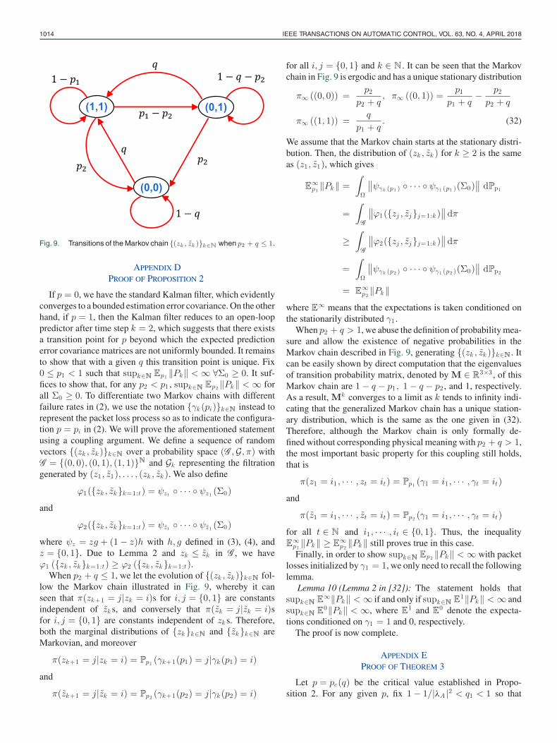
Fig. 9. Transitions of the Markov chain {(zk , zk )}k∈N when p2 + q ≤ 1.

APPENDIX DPROOF OF PROPOSITION 2

If p = 0, we have the standard Kalman filter, which evidentlyconverges to a bounded estimation error covariance. On the otherhand, if p = 1, then the Kalman filter reduces to an open-looppredictor after time step k = 2, which suggests that there existsa transition point for p beyond which the expected predictionerror covariance matrices are not uniformly bounded. It remainsto show that with a given q this transition point is unique. Fix0 ≤ p1 < 1 such that supk∈N Ep1 ‖Pk‖ <∞ ∀Σ0 ≥ 0. It suf-fices to show that, for any p2 < p1 , supk∈N Ep2 ‖Pk‖ <∞ forall Σ0 ≥ 0. To differentiate two Markov chains with differentfailure rates in (2), we use the notation {γk (pi)}k∈N instead torepresent the packet loss process so as to indicate the configura-tion p = pi in (2). We will prove the aforementioned statementusing a coupling argument. We define a sequence of randomvectors {(zk , zk )}k∈N over a probability space (G ,G, π) withG = {(0, 0), (0, 1), (1, 1)}N and Gk representing the filtrationgenerated by (z1 , z1), . . . , (zk , zk ). We also define

ϕ1({zk , zk}k=1:t) = ψzt ◦ · · · ◦ ψz1 (Σ0)

and

ϕ2({zk , zk}k=1:t) = ψzt ◦ · · · ◦ ψz1 (Σ0)

where ψz = zg + (1 − z)h with h, g defined in (3), (4), andz = {0, 1}. Due to Lemma 2 and zk ≤ zk in G , we haveϕ1 ({zk , zk}k=1:t) ≥ ϕ2 ({zk , zk}k=1:t).

When p2 + q ≤ 1, we let the evolution of {(zk , zk )}k∈N fol-low the Markov chain illustrated in Fig. 9, whereby it canseen that π(zk+1 = j|zk = i)s for i, j = {0, 1} are constantsindependent of zk s, and conversely that π(zk = j|zk = i)sfor i, j = {0, 1} are constants independent of zk s. Therefore,both the marginal distributions of {zk}k∈N and {zk}k∈N areMarkovian, and moreover

π(zk+1 = j|zk = i) = Pp1 (γk+1(p1) = j|γk (p1) = i)

and

π(zk+1 = j|zk = i) = Pp2 (γk+1(p2) = j|γk (p2) = i)

for all i, j = {0, 1} and k ∈ N. It can be seen that the Markovchain in Fig. 9 is ergodic and has a unique stationary distribution

π∞ ((0, 0)) =p2

p2 + q, π∞ ((0, 1)) =

p1

p1 + q− p2

p2 + q

π∞ ((1, 1)) =q

p1 + q. (32)

We assume that the Markov chain starts at the stationary distri-bution. Then, the distribution of (zk , zk ) for k ≥ 2 is the sameas (z1 , z1), which gives

E∞p1‖Pk‖ =

∫Ω

∥∥ψγk (p1 ) ◦ · · · ◦ ψγ1 (p1 )(Σ0)∥∥ dPp1

=∫

G

∥∥ϕ1({zj , zj}j=1:k )∥∥dπ

≥∫

G

∥∥ϕ2({zj , zj}j=1:k )∥∥dπ

=∫

Ω

∥∥ψγk (p2 ) ◦ · · · ◦ ψγ1 (p2 )(Σ0)∥∥ dPp2

= E∞p2‖Pk‖

where E∞ means that the expectations is taken conditioned onthe stationarily distributed γ1 .

When p2 + q > 1, we abuse the definition of probability mea-sure and allow the existence of negative probabilities in theMarkov chain described in Fig. 9, generating {(zk , zk )}k∈N . Itcan be easily shown by direct computation that the eigenvaluesof transition probability matrix, denoted by M ∈ R3×3 , of thisMarkov chain are 1 − q − p1 , 1 − q − p2 , and 1, respectively.As a result, Mk converges to a limit as k tends to infinity indi-cating that the generalized Markov chain has a unique station-ary distribution, which is the same as the one given in (32).Therefore, although the Markov chain is only formally de-fined without corresponding physical meaning with p2 + q > 1,the most important basic property for this coupling still holds,that is

π(z1 = i1 , · · · , zt = it) = Pp1 (γ1 = i1 , · · · , γt = it)

and

π(z1 = i1 , · · · , zt = it) = Pp2 (γ1 = i1 , · · · , γt = it)

for all t ∈ N and i1 , · · · , it ∈ {0, 1}. Thus, the inequalityE∞p1‖Pk‖ ≥ E∞

p2‖Pk‖ still proves true in this case.

Finally, in order to show supk∈N Ep2 ‖Pk‖ <∞ with packetlosses initialized by γ1 = 1, we only need to recall the followinglemma.

Lemma 10 (Lemma 2 in [32]): The statement holds thatsupk∈N E∞‖Pk‖ <∞ if and only if supk∈N E1‖Pk‖ <∞ andsupk∈N E0‖Pk‖ <∞, where E1 and E0 denote the expecta-tions conditioned on γ1 = 1 and 0, respectively.

The proof is now complete.

APPENDIX EPROOF OF THEOREM 3

Let p = pc(q) be the critical value established in Propo-sition 2. For any given p, fix 1 − 1/|λA |2 < q1 < 1 so that


supk∈N Eq1 ‖Pk‖ <∞ for all Σ0 ≥ 0. From a symmetricalcoupling argument as the proof of Proposition 2, for anyq1 ≤ q2 < 1, supk∈N Eq2 ‖Pk‖ <∞ also holds for all Σ0 ≥ 0.As a result, pc(q) is a nondecreasing function of q. Consequently,pc(·) yields an inverse function, denoted by qc(·), which is alsonondecreasing. The desired conclusion then follows immedi-ately, e.g., we can simply choose fc(p, q) = pc(q) − p.

APPENDIX FPROOF OF THEOREM 4

We shall first show that

limη→1+

p(η) = p (33)

holds where η > 1 is properly taken so that η2 |λA |2(1 − q) < 1,and

p(η) � sup{p : ∃(K,P ) s.t. L(ηA,K,P, p) < P,P > 0

}

with the notation L(A,K,P, p) used to alter LK (P ) in theproof so as to emphasize the relevance of LK (P ) to A and p.To this end, first note that p(η) is a nonincreasing function ofη. Thus, limη→1+ p(η) must exist. To show the equality in (33),we require the following lemma.

Lemma 11: Suppose X, X > 0 are the solutions to the fol-lowing Lyapunov equations, respectively:

X = (1 − q)AXA′ + Q, η−1X = (1 − q)AXA′ + Q

where Q > 0, 0 < q < 1 and η > 1 are properly taken so thatη(1 − q)|λA |2 < 1. Then, for any ε > 0 there always exists aδ > 0 such that η ≤ 1 + δ implies X ≤ (1 + ε)X.

Proof: First we shall find an upper bound for X and a lowerbound for X . It is straightforward that

X ≥ Q ≥ ‖Q−1‖−1I. (34)

Let d �[(1 − q)|λA |2

]−1/4> 1 and restrict 1 < η ≤ d. By

Lemma 4, we have

X =∞∑i=0

ηi(1 − q)iAiQ(Ai)′ ≤ ‖Q‖∞∑i=0

ηi(1 − q)i‖Ai‖2I

≤ n‖Q‖(1 + 2/ε)2n−2∞∑i=0

di(1 − q)i(|λA | + ε‖A‖)2iI

for any ε > 0. Taking ε = (d−1)|λA |‖A‖ , it yields that X ≤ cd

d−1 ‖Q‖with c = n(1 + 2/ε)2n−2 . Note that X −X is bounded in thefollowing way

X −X = (1 − q)A(X −X)A′

+ (η − 1)[(1 − q)AXA′ + Q

]

≤ (1 − q)A(X −X)A′ + (η − 1)X

...

≤ (1 − q)kAk (X −X)(·)′

+(η − 1)k−1∑i=0

(1 − q)iAiX(Ai)′.

Taking limitation on both sides, we obtain that X −X ≤ (η −1)

∑∞i=0(1 − q)iAiX(Ai)′, which by Lemma 4 and (34) gives

X −X ≤ (η − 1)‖Q‖ cd

d− 1

∞∑i=0

(1 − q)i‖Ai‖2 I

≤ c2d3

(d2 − 1)(d− 1)(η − 1)‖Q‖ I

≤ c2d3

(d2 − 1)(d− 1)(η − 1)‖Q‖‖Q−1‖X

where the last inequality holds because of (34). Due to thepositive definiteness of Q, the assertion follows by letting 1 <η ≤ min

{(d2 −1)(d−1)c2 d3 ‖Q‖‖Q−1 ‖ε+ 1, d

}.

By the definition of p one can verify that for any 0 < ε < pthere always exists at least a p ∈ (p− ε, p) so that there existKand P > 0 satisfying L(A,K,P, p) < P ; otherwise it contra-dicts (13). We take an ε > 0 so that (1 + ε)L(A,K,P, p) < Pstill holds. Then, from Lemma 11, there always exists an η0 > 1satisfying Φη0 ≤ √

1 + εΦ where Φ and Φη0 are the positivedefinite solutions to the following equations, respectively:

Φ = (1 − q)A′ΦA+A′PA,

η−20 Φη0 = (1 − q)A′Φη0A+A′PA.

In addition, there exists an η1 > 1 such that η2Io−21 ≤ √

1 + ε.Letting η = min{η0 , η1}, we have

P > (1 + ε)L(A,K,P, p)

≥ p

Io−1∑i=1

(1 − p)i−1(ηiAi + ηiK(i)C(i))∗(Φη )(·)

which implies that L(ηA,Kη , P, p) < P with Kη �[ηK(1) , · · · , ηIo−1K(Io−1) ] and therefor that p(η) > p− ε. Asε is any positive real number, limη→1+ p(η) = p consequentlyholds. Since ηA has no defective eigenvalues on the unit circle,combining Theorems 1 and 2, we obtain that pc(ηA,C, q) ≥p(η) holds.

To conclude, we also need to establish the following lemma.Lemma 12: For a given recovery rate q satisfying |λA |2(1 −

q) < 1, denote qc(A,C, q) as the critical value of qc for a system(C,A). Then, we have

pc(A,C, q) ≥ limη→1+

pc(ηA,C, q). (35)

Proof: To emphasize the relevance of h(X) and g(X) toA, we will change the notations h(X) and g(X) into h(A,X)and g(A,X), respectively, in the proof. Note that h(ηA,X)


and g(ηA,X) are both nondecreasing function of η > 1, whereη is properly chosen so that η2 |λA |2(1 − q) < 1, since, for all1 ≤ η1 ≤ η2 ≤ 1 + δ and X ≥ 0, one has

h(η2A,X) − h(η1A,X) = (η22 − η2

1 )AXA′ ≥ 0

and

(η2A,X) − g(η1A,X)

= (η22 − η2

1 )(AXA′ −AXC ′(CXC ′ +R)−1CXA′) ≥ 0.

According to the fact that Pk = (1 − γk )h(A,Pk−1) +γkg(A,Pk−1) and that h(A,X) and g(A,X) are nondecreasingfunctions ofX from Lemma 2, we can easily show by inductionthat Pk is also nondecreasing in η. Therefore, the limitation onthe right side of (35) always exists, and then, the conclusionfollows. �

From Lemma 12 and what has been proved previously, it canbe seen that limη→1+ pc(ηA,C, q) and limη→1+ p(η) exist andmoreover that

pc(A,C, q) ≥ limη→1+

pc(ηA,C, q) ≥ limη→1+

p(η) = p

whereby the desired result follows.

ACKNOWLEDGMENT

The authors would like to thank the Associate Editor and theanonymous reviewers for their useful comments and construc-tive suggestions.

REFERENCES

[1] J. Wu, G. Shi, B. D. O. Anderson, and K. J. Johansson, “Stability conditionsand phase transition for Kalman filtering over Markovian channels,” inProc. 34th Chin. Control Conf., Hangzhou, China, 2015, pp. 6721–6728.

[2] S. Tatikonda and S. Mitter, “Control under communication constraints,”IEEE Trans. Automat. Control, vol. 49, no. 7, pp. 1056–1068, Jul. 2004.

[3] J. Hespanha, P. Naghshtabrizi, and Y. Xu, “A survey of recent resultsin networked control systems,” Proc. IEEE, vol. 95, no. 1, pp. 138–162,Jan. 2007.

[4] G. N. Nair, F. Fagnani, S. Zampieri, and R. J. Evans, “Feedback controlunder data rate constraints: An overview,” Proc. IEEE, vol. 95, no. 1,pp. 108–137, Jan. 2007.

[5] W. S. Wong and R. W. Brockett, “Systems with finite communicationbandwidth–Part I: State estimation problems,” IEEE Trans. Automat. Con-trol, vol. 42, no. 9, pp. 1294–1299, Sep. 1997.

[6] W. S. Wong and R. W. Brockett, “Systems with finite communicationbandwidth–Part II: Stabilization with limited information feedback,” IEEETrans. Automat. Control, vol. 44, no. 5, pp. 1049–1053, May 1999.

[7] R. W. Brockett and D. Liberzon, “Quantized feedback stabilizationof linear systems,” IEEE Trans. Automat. Control, vol. 45, no. 7,pp. 1279–1289, Jul. 2000.

[8] G. N. Nair and R. J. Evans, “Communication-limited stabilization of linearsystems,” in Proc. 39th IEEE Conf. Decis. Control, 2000, pp. 1005–1010.

[9] N. Elia and S. Mitter, “Stabilization of linear systems with limited infor-mation,” IEEE Trans. Automat. Control, vol. 46, no. 9, pp. 1384–1400,Sep. 2001.

[10] H. Ishii and B. A. Francis, “Quadratic stabilization of sampled-data sys-tems with quantization,” Automatica, vol. 39, pp. 1793–1800, 2003.

[11] M. Fu and L. Xie, “The sector bound approach to quantized feedbackcontrol,” IEEE Trans. Automat. Control, vol. 50, no. 11, pp. 1698–1711,Nov. 2005.

[12] P. Minero, M. Franceschetti, S. Dey, and G. N. Nair, “Data rate theorem forstabilization over time-varying feedback channels,” IEEE Trans. Automat.Control, vol. 54, no. 2, pp. 243–255, Feb. 2009.

[13] P. Minero, L. Coviello, and M. Franceschetti, “Stabilization over Markovfeedback channels: The general case,” IEEE Trans. Automat. Control,vol. 58, no. 2, pp. 349–362, Feb. 2013.

[14] A. C. Harvey, Forecasting, Structural Time Series Models and the KalmanFilter. Cambridge, U.K.: Cambridge Univ. Press, 1990.

[15] S. Haykin, Kalman Filtering and Neural Networks, vol. 47. New York,NY, USA: Wiley, 2004.

[16] B. Sinopoli, L. Schenato, M. Franceschetti, K. Poola, M. Jordan, and S.Sastry, “Kalman filtering with intermittent observations,” IEEE Trans.Automat. Control, vol. 49, no. 9, pp. 1453–1464, Sep. 2004.

[17] B. Sinopoli, L. Schenato, M. Franceschetti, K. Poolla, and S. S. Sastry,“Optimal control with unreliable communication: The TCP case,” in Proc.Amer. Control Conf., 2005, pp. 3354–3359.

[18] O. C. Imer, S. Yuksel, and T. Basar, “Optimal control of LTI sys-tems over unreliable communication links,” Automatica, vol. 42, no. 9,pp. 1429–1439, 2006.

[19] B. Sinopoli, L. Schenato, M. Franceschetti, K. Poolla, and S. Sastry, “Op-timal linear LQG control over lossy networks without packet acknowl-edgment,” Asian J. Control, vol. 10, no. 1, pp. 3–13, 2008.

[20] L. Schenato, B. Sinopoli, M. Franceschetti, K. Poolla, and S. Sastry,“Foundations of control and estimation over lossy networks,” Proc. IEEE,vol. 95, no. 1, pp. 163–187, Jan. 2007.

[21] K. Plarre and F. Bullo, “On Kalman filtering for detectable systems withintermittent observations,” IEEE Trans. Automat. Control, vol. 54, no. 2,pp. 386–390, Feb. 2009.

[22] Y. Mo and B. Sinopoli, “Towards finding the critical value for Kalmanfiltering with intermittent observations,” arXiv:1005.2442, 2010.

[23] E. N. Gilbert, “Capacity of a burst-noise channel,” Bell Syst. Tech. J.,vol. 39, no. 5, pp. 1253–1265, 1960.

[24] E. Elliott, “Estimates of error rates for codes on burst-noise channels,”Bell Syst. Tech. J., vol. 42, no. 5, pp. 1977–1997, 1963.

[25] H. S. Wang and N. Moayeri, “Finite-state Markov channel–A useful modelfor radio communication channels,” IEEE Trans. Veh. Technol., vol. 44,no. 1, pp. 163–171, Feb. 1995.

[26] Q. Zhang and S. A. Kassam, “Finite-state Markov model for rayleighfading channels,” IEEE Trans. Commun., vol. 47, no. 11, pp. 1688–1692,Nov. 1999.

[27] A. Willig, “Recent and emerging topics in wireless industrial communica-tions: A selection,” IEEE Trans. Ind. Informat., vol. 4, no. 2, pp. 102–124,May 2008.

[28] M. Huang and S. Dey, “Kalman filtering with Markovian packet lossesand stability criteria,” in Proc. 45th IEEE Conf. Decis. Control, 2006,pp. 5621–5626.

[29] M. Huang and S. Dey, “Stability of Kalman filtering with Markovianpacket losses,” Automatica, vol. 43, pp. 598–607, 2007.

[30] L. Xie and L. Xie, “Peak covariance stability of a random Riccati equa-tion arising from Kalman filtering with observation losses,” J. Syst. Sci.Complexity, vol. 20, no. 2, pp. 262–272, 2007.

[31] L. Xie and L. Xie, “Stability of a random Riccati equation with Marko-vian binary switching,” IEEE Trans. Automat. Control, vol. 53, no. 7,pp. 1759–1764, Aug. 2008.

[32] K. You, M. Fu, and L. Xie, “Mean square stability for Kalman filtering withMarkovian packet losses,” Automatica, vol. 47, no. 12, pp. 2647–2657,2011.

[33] L. Shi, M. Epstein, and R. M. Murray, “Kalman filtering over a packet-dropping network: A probabilistic perspective,” IEEE Trans. Automat.Control, vol. 55, no. 3, pp. 594–604, Mar. 2010.

[34] Y. Mo and B. Sinopoli, “Kalman filtering with intermittent observa-tions: Tail distribution and critical value,” IEEE Trans. Automat. Control,vol. 57, no. 3, pp. 677–689, Mar. 2012.

[35] S. Kar, B. Sinopoli, and J. M. Moura, “Kalman filtering with intermittentobservations: Weak convergence to a stationary distribution,” IEEE Trans.Automat. Control, vol. 57, no. 2, pp. 405–420, Feb. 2012.

[36] A. Censi, “Kalman filtering with intermittent observations: Convergencefor semi-Markov chains and an intrinsic performance measure,” IEEETrans. Automat. Control, vol. 56, no. 2, pp. 376–381, Feb. 2011.

[37] L. Xie, “Stochastic comparison, boundedness, weak convergence, andergodicity of a random Riccati equation with Markovian binary switching,”SIAM J. Control Optim., vol. 50, no. 1, pp. 532–558, 2012.

[38] R. Durrett, Probability: Theory and Examples. Cambridge, U.K.:Cambridge Univ. Press, 2010.

[39] R. A. Horn and C. R. Johnson, Matrix Analysis. Cambridge, U.K.:Cambridge Univ. Press, 2012.

[40] N. Xiao, L. Xie, and M. Fu, “Kalman filtering over unreliable communi-cation networks with bounded Markovian packet dropouts,” Int. J. RobustNonlinear Control, vol. 19, no. 16, pp. 1770–1786, 2009.

[41] V. Solo, “One step ahead adaptive controller with slowly time-varyingparameters,” Dept. of EECS, John Hopkins Univ., Baltimore, MD, USA,Tech. Rep., 1991.


[42] O. L. V. Costa and M. Fragoso, “Comments on “stochastic stability ofjump linear systems”,” IEEE Trans. Automat. Control, vol. 49, no. 8,pp. 1414–1416, Aug. 2004.

[43] P. Lancaster and L. Rodman, Algebraic Riccati Equations. London, U.K.:Oxford Univ. Press, 1995.

Junfeng Wu received the B.Eng. degree fromthe Department of Automatic Control, ZhejiangUniversity, Hangzhou, China, and the Ph.D. de-gree in electrical and computer engineering fromHong Kong University of Science and Technol-ogy, Hong Kong, in 2009, and 2013, respectively.

From September to December 2013, he was aResearch Associate in the Department of Elec-tronic and Computer Engineering, Hong KongUniversity of Science and Technology. From Jan-uary 2014 to June 2017, he was a Postdoctoral

Researcher in the ACCESS (Autonomic Complex Communication nEt-works, Signals and Systems) Linnaeus Center, School of Electrical En-gineering, KTH Royal Institute of Technology, Stockholm, Sweden. Heis currently in the College of Control Science and Engineering, Zhe-jiang University, Hangzhou, China. His research interests include net-worked control systems, state estimation, and wireless sensor networks,multiagent systems.

Dr. Wu received the Guan Zhao-Zhi Best Paper Award at the 34thChinese Control Conference in 2015. He was selected to the national“1000-Youth Talent Program” of China in 2016.

Guodong Shi received the B.Sc. degree inmathematics and applied mathematics from theSchool of Mathematics, Shandong University,Ji’nan, China, and the Ph.D. degree in sys-tems theory from the Academy of Mathemat-ics and Systems Science, Chinese Academyof Sciences, Beijing, China, in 2005 and 2010,respectively.

From 2010 to 2014, he was a PostdoctoralResearcher in the ACCESS Linnaeus Centre,KTH Royal Institute of Technology, Stockholm,

Sweden. Since May 2014, he has been with the Research School of En-gineering, The Australian National University, Canberra, ACT, Australia,where he is now a Senior Lecturer and Future Engineering ResearchLeadership Fellow. His research interests include distributed control sys-tems, quantum networking and decisions, and social opinion dynamics.

Brian D. O. Anderson (M’66–SM’74–F’75–LF’07) was born in Sydney, Australia. Hereceived the degree in mathematics and elec-trical engineering from Sydney University, Syd-ney, NSW, Australia, and the Ph.D. degree inelectrical engineering from Stanford University,Stanford, CA, USA, in 1966.

He is an Emeritus Professor in the AustralianNational University, Canberra, ACT, Australia(having retired as a Distinguished Professor in2016), a Distinguished Professor in Hangzhou

Dianzi University, and a Distinguished Researcher in the National In-formation and Communications Technology Australia. He is a PastPresident of the International Federation of Automatic Control and theAustralian Academy of Science. His research interests include dis-tributed control, sensor networks, and econometric modeling.

Dr. Anderson is a Fellow of the Australian Academy of Science, theAustralian Academy of Technological Sciences and Engineering, theRoyal Society, and a Foreign Member of the U.S. National Academy ofEngineering. He received the IEEE Control Systems Award of 1997, the2001 IEEE James H. Mulligan, Jr., Education Medal, and the Bode Prizeof the IEEE Control System Society in 1992, as well as several IEEE andother best paper prizes. He holds honorary doctorates from a numberof universities, including Universit Catholique de Louvain, Belgium, andETH, Zrich.

Karl Henrik Johansson (F’13) received theM.Sc. and Ph.D. degrees in electrical engineer-ing from Lund University, Lund, Sweden.

He is the Director of the Stockholm Strate-gic Research Area, Information and Communi-cations Technology, The Next Generation, anda Professor in the School of Electrical En-gineering, KTH Royal Institute of Technology,Stockholm, Sweden. He has held visiting posi-tions at the University of California, Berkeley, theCalifornia Institute of Technology, the NTU, the

Institute of Advanced Studies, Hong Kong University of Science andTechnology, and the Norwegian University of Science and Technology.He is also an IEEE Distinguished Lecturer. His research interests includenetworked control systems, cyber-physical systems, and applications intransportation, energy, and automation.

Dr. Johansson is a member of the IEEE Control Systems SocietyBoard of Governors, the International Federation of Automatic Con-trol (IFAC) executive board, the European Control Association Council,and the Royal Swedish Academy of Engineering Sciences. He receivedseveral best paper awards and other distinctions, including a ten-yearWallenberg Scholar Grant, a Senior Researcher Position with theSwedish Research Council, the Future Research Leader Award fromthe Swedish Foundation for Strategic Research, and the triennial YoungAuthor Prize from the IFAC.

kalman filtering over gilbert–elliott channels: stability

Documents