kantian optimization: an approach to cooperative …
TRANSCRIPT

KANTIAN OPTIMIZATION: AN APPROACH TO COOPERATIVE BEHAVIOR
By
John E. Roemer
March 2012 Revised October 2013
COWLES FOUNDATION DISCUSSION PAPER NO. 1854R
COWLES FOUNDATION FOR RESEARCH IN ECONOMICS YALE UNIVERSITY
Box 208281 New Haven, Connecticut 06520-8281
http://cowles.econ.yale.edu/
September 1, 2013
“Kantian optimization: An approach to cooperative behavior” 1
by2
John E. Roemer13
4
Abstract. Although evidence accrues in biology, anthropology and experimental 5
economics that homo sapiens is a cooperative species, the reigning assumption in 6
economic theory is that individuals optimize in an autarkic manner (as in Nash and 7
Walrasian equilibrium). I here postulate a cooperative kind of optimizing behavior, 8
called Kantian. It is shown that in simple economic models, when there are negative 9
externalities (such as congestion effects from use of a commonly owned resource) or 10
positive externalities (such as a social ethos reflected in individuals’ preferences), 11
Kantian equilibria dominate Nash-Walras equilibria in terms of efficiency. While 12
economists schooled in Nash equilibrium may view the Kantian behavior as utopian, 13
there is some – perhaps much -- evidence that it exists. If cultures evolve through group 14
selection, the hypothesis that Kantian behavior is more prevalent than we may think is 15
supported by the efficiency results here demonstrated. 16
17
Key words: Kantian equilibrium, social ethos, implementation 18
JEL codes: D60, D62, D64, C70, H30 19
20
2122
23
24
25
1 Department of political science and Cowles Foundation, Yale University. My main debt is to Joaquim Silvestre, with whom I have discussed these ideas for many years. I also thank the following, for their suggestions and help: Roger Howe, François Maniquet, Juan Moreno-Ternero, Joseph Ostroy, Larry Samuelson, Rajiv Sethi, Joel Sobel, and referees for this journal.
1
1. Introduction 26
Recent work in contemporary social science and evolutionary biology emphasizes 27
that homo sapiens is a cooperative species. In evolutionary biology, scientists are 28
interested in explaining how cooperation and ‘altruism’ may have developed among 29
humans through natural selection. In economics, there is now a long series of 30
experiments whose results are often explained by the hypothesis that individuals are to 31
some degree altruistic. A recent summary of the state-of-the-art in experimental 32
economics, anthropology, and evolutionary biology is provided by Bowles and Gintis 33
(2011). Rabin (2006) provides a summary of the evidence for altruism from 34
experimental economics. An anthropological view is provided in Henrich and Henrich 35
(2007). Alger and Weibull (2012) model the evolution of altruism, and provide a useful 36
bibliography.37
Altruism may induce behavior that appears to be cooperative, but altruism and 38
cooperation have different motivations. Altruism, at least when it is intentional in 39
humans, is motivated by a desire to improve the welfare of others, while cooperation may 40
be motivated (only) by the desire to help oneself. (For example, workers in a firm 41
cooperate, but each may do so because she realizes that cooperative behavior advances 42
her own welfare.) There is an important line of research, conducted by Ostrom (1990) 43
and her collaborators, arguing that, in many small societies, people figure out how to 44
cooperate to avoid, or solve, the ‘tragedy of the commons.’ That tragedy may be 45
summarized as follows. Imagine a lake which is owned in common by a group of fishers, 46
who each possess preferences over fish and leisure, and perhaps differential skill (or sizes 47
of boats) in (or for) fishing. The lake produces fish with decreasing returns with respect 48
to the fishing labor expended upon it. In the game in which each fisher proposes as her 49
strategy a fishing time, it is well known that the Nash equilibrium is Pareto inefficient: 50
there are congestion externalities, and all would be better off were they able to design a 51
decrease, of a certain kind, in everyone’s fishing. Ostrom studied many such societies, 52
and maintained that many or most of them learn to regulate ‘fishing,’ without privatizing 53
the ‘lake.’ Somehow, the inefficient Nash equilibrium is avoided. This example is not 54
one in which fishers care about other fishers (necessarily), but it is one in which 55
cooperation is organized to deal with a negative externality of autarkic behavior.56
2
The ethos that motivates cooperation is called solidarity. Merriam-Webster’s 57
dictionary defines solidarity as ‘unity (as a group or class) that produces or is based on 58
community of interests or objectives.’ There is no mention of altruism: we do not 59
cooperate because we care about others, but because we recognize we are all in the same 60
boat, and cooperation will advance each individual interest. Of course, if altruism exists, 61
it may also motivate cooperation, but I wish to emphasize that cooperation does not 62
require altruism. 63
Ostrom’s observations pertain to small societies. In large economies, we 64
observe the evolution of the welfare state, supported by considerable degrees of taxation 65
of market earnings. It is conventionally argued that the successful welfare states had 66
their genesis in solidarity: they provided insurance which was in everyone’s self-interest.67
It was easier to organize welfare states where citizens were ethnically and linguistically 68
homogeneous, because the ‘unity’ which Merriam-Webster refers to was more evident in 69
this case. We do not need to invoke altruism among the citizens of Nordic societies to 70
explain the welfare state: in other words, their homogeneity was the source of their 71
recognition of common interests, but it need not have induced altruism to generate the 72
welfare state. 73
There is, however, also an argument that welfare states expand after wars as a 74
reward to returning soldiers ; see Scheve and Stasavage[2012]. Perhaps altruism 75
develops in a population as a result of their participation in a cooperative venture: we 76
identify more with others when we succeed in cooperating, and that identification may 77
lead to altruism. Or we feel soldiers deserve a reward for having fought the war.78
Redistributive taxation appears to be at least to some degree a polity’s reaction to the 79
material deprivation of a section of society, which many view as undeserved, and desire 80
to redress. To the extent that welfare states provide insurance which it is rational for self-81
interested agents to desire, it is a manifestation of cooperation; to the extent that citizens 82
support the welfare state to redress unjust inequality, it is a manifestation of altruism, or 83
at least of a sense of justice. Regardless of the motive, as is well-known, redistributive 84
taxation induces, to some degree, allocative inefficiency. I will argue that this is due in 85
large part to non-cooperative behavior of individual workers when they face the tax 86
regime. Each worker is computing his optimal labor supply in the Nash fashion: that is, 87
3
assuming that all others are holding their labor supplies fixed. 88
Among economists, there have been a number of strategies to explain behavior 89
that is not easily explained as the Nash equilibrium of the game that agents appear to be 90
playing. Ostrom explains the avoidance of the tragedy of the commons among ‘fishing 91
communities’ by the imposition of punishment of those who deviate from the cooperative 92
behavior: in other words, the payoffs of the game are changed so that it becomes a Nash 93
equilibrium for each fisher to cooperate. This is also the argument that Mancur Olson 94
(1965) employs to explain cooperation: unions, for example, get workers to cooperate by 95
offering side payments and punishments for those who deviate. In experimental 96
economics, when individuals often do not play what appears to be the Nash equilibrium 97
of a game ( dictator and ultimatum games, for example) , there are a number of moves.98
Perhaps individuals are using rules of thumb that are associated with strategies that are 99
equilibria in repeated games, even though the game in the laboratory is not repeated. Or 100
perhaps players have other-regarding preferences: they are to some degree altruistic. Or 101
perhaps they have a sense of morality, which can be viewed as a kind of preference – a 102
player feels better when, in the dictator game, she gives something to the opponent. Or, 103
in the ultimatum game, the proposer offers a substantial amount to the opponent because 104
she believes the opponent does not have classical preferences – that is, Opponent will 105
reject an ‘unfair’ offer. Outcomes are then explained as Nash equilibria of games whose 106
players have non-classical (i.e., non-self-interested) preferences.107
Here, I introduce another approach. I propose that we can explain cooperation by 108
observing that players may be optimizing in a non-classical (that is, non-Nash) manner.109
This leads to a class of equilibrium concepts that I call Kantian equilibria. Briefly, with 110
Kantian optimization, agents ask themselves, at a particular set of actions/strategies in a 111
game: If I were to deviate from my stipulated action, and all others were to deviate in like 112
manner from their stipulated actions, would I prefer the consequences of the new action 113
profile? I denote this kind of thinking Kantian because an individual only deviates in a 114
particular way, at an action profile, if he would prefer the situation in which his action 115
were universalized – that is to say, he’d prefer the action profile where all make the kind 116
of deviation he is contemplating. Each agent evaluates not the profile that would result 117
if only he deviated, but rather the profile of actions that would result if all deviated in 118
4
similar fashion. Kant’s categorical imperative says: Take those and only those actions 119
that are universalizable, meaning that the world would be better (according to one’s own 120
preferences) were one’s behavior universalized. It is important that the new action 121
profile be evaluated with one’s own preferences, which need not be altruistic.122
There is a distinction, then, between the approach of behavioral economics, which 123
has by and large focused on amending preferences from self-interested ones to altruistic 124
or other-regarding ones, or ones in which players possess a sense of justice, to the 125
approach I describe, which amends optimizing behavior, but does not (necessarily) fiddle 126
with preferences. Of course, one could be even more revisionist, and amend both127
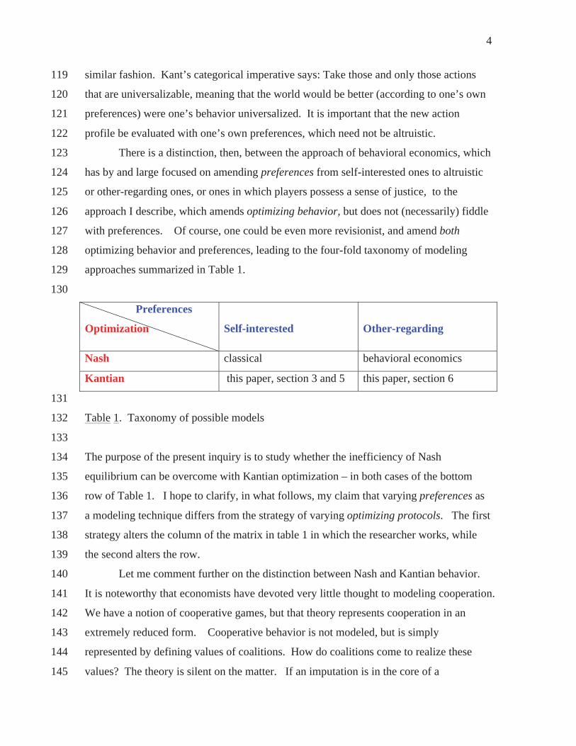
optimizing behavior and preferences, leading to the four-fold taxonomy of modeling 128
approaches summarized in Table 1. 129
130
Preferences
Optimization Self-interested Other-regarding
Nash classical behavioral economics
Kantian this paper, section 3 and 5 this paper, section 6
131
Table 1. Taxonomy of possible models 132
133
The purpose of the present inquiry is to study whether the inefficiency of Nash 134
equilibrium can be overcome with Kantian optimization – in both cases of the bottom 135
row of Table 1. I hope to clarify, in what follows, my claim that varying preferences as 136
a modeling technique differs from the strategy of varying optimizing protocols. The first 137
strategy alters the column of the matrix in table 1 in which the researcher works, while 138
the second alters the row. 139
Let me comment further on the distinction between Nash and Kantian behavior. 140
It is noteworthy that economists have devoted very little thought to modeling cooperation. 141
We have a notion of cooperative games, but that theory represents cooperation in an 142
extremely reduced form. Cooperative behavior is not modeled, but is simply 143
represented by defining values of coalitions. How do coalitions come to realize these 144
values? The theory is silent on the matter. If an imputation is in the core of a 145
5
cooperative game, it is, a fortiori, Pareto efficient: typically, one is concerned with 146
whether cooperative games contain non-empty cores, but the behavior which leads to an 147
imputation in the core is typically not studied. A major exception to this claim is the 148
theorem that non-cooperative, autarkic optimizing behavior, in a perfectly competitive 149
market economy, induces an equilibrium that lies in the core of an associated game. But 150
this is an exception to my claim, not the rule. In contrast, the Shapley value of a convex 151
cooperative game is in the core: but I do not think anyone derives the Shapely value as 152
the outcome of optimizing behavior of individuals. 153
I wish to propose that Kantian optimization can be viewed as a model of 154
cooperation. As a Kantian optimizer, I hold a norm that says: “If I want to deviate from 155
a contemplated action profile (of my community’s members), then I may do so only if I 156
would have all others deviate ‘in like manner.’” I have not spelled out what the phrase 157
‘in like manner’ means, as yet – that will comprise the details of this paper. Contrast 158
this kind of thinking with the autarkic thinking postulated in Nash behavior – I change 159
my action by myself, assuming that others in my community stand pat.160
In section 2, the economic environment for this inquiry is specified. Section 3 161
introduces two examples of Kantian optimization and proves that they produce Pareto 162
efficient outcomes – they resolve different kinds of commons’ tragedies that can afflict 163
societies living in these economic environments. Section 4 takes up two possible 164
objections to the approach, and argues more explicitly that Kantian optimization is not 165
equivalent to altering agents’ preferences. Section 5 presents a more general theory of 166
Kantian optimization. Section 6 introduces altruism into agents’ preferences, and studies 167
whether Kantian optimization will continue to produce Pareto efficient outcomes.168
Section 7 contains a brief discussion of the existence of Kantian equilibria, and their 169
dynamics. Section 8 concludes2.170
2 I originally proposed a definition of Kantian equilibrium in Roemer (1996), and showed
its relationship to the ‘proportional solution, ’ of Roemer and Silvestre (1993). In
Roemer (2010), I investigated a special case of Kantian equilibrium, that I now call
multiplicative Kantian equilibrium. The present paper shows that there are many
versions of Kantian optimization, and characterizes when they deliver efficient outcomes
6
171
2. The economic environment 172
There is a concave, differentiable production function G that produces a single 173
output from a single input, called effort. Effort is supplied by individuals; it may differ in 174
intensity or efficiency units, but effort, measured in efficiency units, can be aggregated 175
across individuals. We assume, except in section 6, that there are a finite number of 176
individuals, n. If the sum of individual efforts is ES then total production is G(ES ) .177
We denote the effort expended by an agent of type by E . It is assumed that effort is 178
unbounded above but bounded below by zero. Let the class of such production functions 179
be denoted G.180
An individual of type has preferences represented by a utility function 181
u (x,E) where x is consumption and E is effort. A person’s utility depends only her 182
own consumption and effort, until section 6 below.183
An allocation rule is a mapping X : +n ×G +
n . If the vector of efforts is 184
E = (E1,...,E ,...,En ) then X(E,G) is the allocation of output to individuals under the 185
rule X . If we write X = (X1,...,Xn ) as a vector of real-valued functions, then 186
X (E1,...,En ,G) is the amount of output produced which agent receives. Thus, it is 187
identically true that for any non-wasteful allocation rule, X (E1,...,En ,G) G(ES ) . 188
We will also at times write allocation rules in terms of the shares of output that 189
they induce: that is an allocation rule X induces a vector of shares assigned to individuals, 190
given by X (E,G) = (E,G)G(ES ) . Of course, 1 . 191
An economic environment is specified by a profile of utility functions and a 192
production function: e = (u1,...,un ,G) . An economy is a pair (e,X) . An economy 193 in the presence of the various kinds of externalities in which Nash equilibrium performs
poorly. As well as extending the results of Roemer (2010) in a number of ways, this
paper offers a clearer argument about the distinction between preferences and
optimization protocols.

7
induces a game among the population: for any vector of efforts, each can compute her 194
utility. That is, define the payoff functions {V } by: 195
V (E1,...,En ) = u (X (E,G),E ), where E = (E1,...,En ) . (2.1) 196
For example, consider the fishing economy described in section 1. It is assumed that 197
each fisher keeps his catch. Thus, statistically speaking, the amount of fish received by 198
fisher will be proportional to the fraction of total labor, in efficiency units, that he 199
expends. The allocation rule is given by: 200
,Pr (E1,...,En ) = EES . (2.2)3201
For obvious reasons, this is called the proportional (Pr) allocation rule. The game 202
induced by the proportional allocation rule has payoff functions: 203
V (E1,...,En ) = u (EES G(E
S ),E ) . (2.3) 204
The ‘tragedy of the commons’ is the statement that if G is strictly concave, then the Nash 205
equilibria of the game defined by (2.3) are Pareto inefficient: indeed all would be better 206
off by suitable reductions in their effort from the Nash effort allocation. 207
Another important rule is the equal division allocation rule, given by: 208
,ED (E1,...,En ) = 1n
, (2.4) 209
and a third class of rules are the Walrasian allocation rules, given by: 210
,Wa (E1,...,En ,G) = G (ES )
G(ES )E + (1
G (ES )ES
G(ES )) , (2.5) 211
in which an agent receives output equal to her effort multiplied by the Walrasian wage 212
plus her share ( ) of profits. Note that the Walrasian shares do depend upon G,213
unlike the proportional and equal-division shares, and this illustrates why, in general, we 214
allow to depend upon G as well as the effort vector. 215
Denote the class of economic environments (u1,...,un ,G) in which n is finite, 216
G G , and the u are concave, differentiable functions, by . Denote the sub-class 217
of economic environments were G is linear by . 218
3 For this rule, the shares do not depend upon G.
E0, fin
L0, fin

8
3. Kantian equilibrium in non-altruistic economies219
220
We may formalize the idea of Kantian optimization as follows. Let {V } be a 221
set of payoff functions for a game played by types , where the strategy of each player is 222
a non-negative effort E , and E is the effort profile of the players. A multiplicative223
Kantian equilibrium is an effort profile E* such that nobody would prefer that everybody 224
alter his effort by the same non-negative factor. That is: 225
( )( r 0)(V (E* V (rE* )) (3.1) 226
227
In Roemer (1996, 2010), this concept was simply called ‘Kantian equilibrium.’ 228
The remarkable feature of multiplicative Kantian equilibrium is that it resolves 229
the tragedy of the commons in the fishers’ economy. It is proved in the two citations just 230
mentioned that if a strictly positive effort allocation is a multiplicative Kantian 231
equilibrium in the game defined by (2.3), then it is Pareto efficient in the economy 232
e = (u,G) . This is a stronger statement than saying the allocation is efficient in the game 233
: for in the game, only certain types of allocation are permitted – ones in which fish 234
are distributed in proportion to effort expended. But the economy defines any allocation 235
as feasible, as long as x = G(ES ) . So Kantian behavior, if adopted by individuals, 236
resolves the tragedy of the commons.237
The intuition is that the Kantian counterfactual (that each agent considers only 238
deviations from an effort allocation if all deviate by a common factor) forces each to 239
internalize the externality associated with the congestion effect of his own fishing. It is 240
not obvious that multiplicative Kantian equilibrium will internalize the externality in 241
exactly the right way – to produce efficiency – but it does.242
A proportional solution in the fisher economy is defined as an allocation 243
(x,E) = (x1,..., xn ,E1,...,En ) with two properties: 244
(i) for all , x = EES G(ES ) , and 245
(ii) (x,E) is Pareto efficient. 246
{V }

9
The proportional solution was introduced in Roemer and Silvestre (1993), although the 247
concept of (multiplicative) Kantian equilibrium came later. The proportional solutions of 248
the fisher economy are exactly its positive multiplicative Kantian equilibria (see theorem 249
3 below). In the small societies which Ostrom has studied, which are (in the formal 250
sense) usually ‘economies of fishers’ where each individual ‘keeps his catch,’ she argues 251
that internal regulation assigns ‘fishing times’ that often engender a Pareto efficient 252
allocation. If this is so, these allocations are proportional solutions, and therefore (by the 253
theorem just quoted) they are multiplicative Kantian equilibria in the game where 254
participating fishers/hunters/miners propose labor times for accessing a commonly owned 255
resource. This suggests that small societies discover their multiplicative Kantian 256
equilibria. Ostrom (1990), however, does not provide any evidence for Kantian thinking 257
among citizens of these societies: as mentioned earlier, she explains these good 258
allocations as Nash equilibria of games with altered payoffs. Knowing the theory of 259
multiplicative Kantian equilibrium, one is tempted to ask whether a ‘Kantian 260
optimization protocol’ exists in these small societies, which leads to the discovery of the 261
Pareto efficient equilibrium. 262
I now introduce a second Kantian protocol which leads to a notion of additive263
Kantian equilibrium4. An effort profile E is an additive Kantian equilibrium if and only if 264
no individual would have all individuals add the same amount of effort (positive or 265
negative) to everyone’s present effort. That is: 266
( )( r infE )(V (E) V (E + r)) , (3.2) 267
where E + r is the effort profile in which the effort of type individuals is E + r . The 268
lower bound on r is necessary to avoid negative efforts. Additive Kantian equilibrium 269
again postulates that each person ‘internalizes’ the effects of his contemplated change in 270
effort, but now the variation is additive rather than multiplicative. 271
In the sequel, I will denote these two kinds of Kantian behavior as and . 272
We have: 273
274
4 This variation of Kantian equilibrium was proposed to me by J. Silvestre in 2004.
K K +

10
Theorem 1 Any strictly positive equilibrium with respect to the proportional 275
allocation rule is Pareto efficient on the domain . Any strictly positive 276
equilibrium with respect to the equal-division allocation rule is Pareto efficient on the 277
domain . 278
Proof:279
1. Let E = (E1,...,En ) be a strictly positive equilibrium w.r.t. the proportional allocation 280
rule Pr . The first-order condition stating this fact is: 281
( )d
dr r=1
u (rE
rES G(rES ),rE ) = 0, (3.3) 282
which means: 283
( )(u1E
ES G (ES )ES + u2E ) = 0 . (3.4) 284
Since E > 0 , divide through (3.4) by E , giving: 285
( )(u2u1
= G (ES )) . (3.5) 286
Eqn. (3.5) states that the marginal rate of substitution between income and effort is, for 287
every agent, equal to the marginal rate of transformation, which is exactly the condition 288
for Pareto efficiency at an interior solution. This proves the first claim. 289
2. For the second claim, let E be a equilibrium w.r.t. the equal-division allocation 290
rule for any economy in . Then: 291
( )(d
dr r=0
u(G(ES + nr)
n,E + r) = 0) , (3.6) 292
which expands to: 293( )(u1 G (ES )+ u2 = 0) . (3.7) 294
(Strict positivity of E is here used so that the range of r includes a small neighborhood of 295
zero.) Clearly (3.7) implies (3.5), and again the allocation is Pareto efficient. 296
Examine the proof of the first part of this proposition, and compare the reasoning 297
that agents who are Kantian employ to Nash reasoning. When a fisher contemplates 298
increasing his effort on the lake by 10%, she asks herself, “How would I like it if 299
everyone increased his effort by 10%?” She is thereby forced to internalize the 300
externality that her increased labor would impose on others, when G is strictly concave.301
K ×
E0, fin K +
E0, fin
K +
ED E
0, fin
11
A similar story applies to the additive Kantian equilibrium with respect to the 302
equal-division rule. The Nash equilibrium of the game induced by the equal division 303
rule is Pareto inefficient, as long as G is strictly concave – but in this case, agents apply 304
too little effort at the Nash allocation. But with the K + optimization protocol, agents 305
internalize the effect of their working too little. The equal-division allocation rule is 306
often said to apply to hunting economies: unlike fishers, when tribes hunted for big game, 307
it was common to divide the catch equally among all. Hunting economies, using the 308
equal-division rule, will be plagued by the inefficiency of individuals shirking (taking a 309
nap behind a bush while others carry on), but their problem can be resolved if all use the 310
additive Kantian protocol. Some of the early Israeli kibbutzim used the equal division 311
rule: regardless of efforts expended, the product was divided equally among households312
(or perhaps in proportion to family size). An additive Kantian optimization protocol 313
would therefore have generated Pareto efficient allocations. 314
Theorem 1 states that each method of Kantian optimization (multiplicative or 315
additive) engenders Pareto efficient results in the games induced by particular allocation 316
rules (proportional, equal division). Although generally Kantian optimization forces 317
agents to internalize externalities associated with strictly concave production functions in 318
these economic environments, the optimization protocols do not completely resolve the 319
inefficiencies associated with these externalities except when the allocation rule is the 320
right one.321
We emphasize that, in Kantian optimization, agents evaluate deviations from their 322
own viewpoints, as in Nash optimization. They do not put themselves in the shoes of 323
others, as they do in Rawls’s original position, or in Harsanyi’s (1977) thought 324
experiment in which agents employ empathy. In this sense, Kantian behavior requires 325
less of a displacement from self than ‘veil-of-ignorance’ thought experiments require.326
Agents require no empathy to conduct Kantian optimization: what changes from Nash 327
behavior is the supposition about the counterfactual.328
It remains to ask, when we discover an example of a society that appears to 329
implement one of these allocation rules in a Pareto efficient manner, whether Kantian 330
thinking among its members plays a role in maintaining its stability. This is an empirical 331

12
question. Just as a Nash equilibrium is self-enforcing, so a Kantian allocation will be 332
self-enforcing if the players in the game employ Kantian optimization.333
We close this section with another example of how Kantian optimization can 334
overcome inefficiencies – this time, with respect to income taxation. Suppose G is linear: 335
G(x) = ax , some a > 0 . Suppose each worker is paid his marginal product per unit 336
effort (which is a). The affine tax rule for tax rate t is given by the allocation: 337
X (E1,...,En ) = (1 t)aE + ta ES
n . (3.8) 338
We know that the Nash equilibrium in the game induced by this allocation rule is Pareto 339
inefficient for any t > 0 : this is the familiar deadweight loss of taxation. But we have: 340
341
Theorem 2 On the domain of economies , the strictly positive K + equilibria with 342
respect to the affine tax rules are Pareto efficient, for any t [0,1] . 343
Proof:344
The vector of efforts E comprises a strictly positive K + in such an economy exactly 345
when:346
( )(d
dr r=0
u ((1 t)a(E + r)+ t a(ES + nr)n
,E + r) = 0) , (3.9) 347
which expands to: 348
u1 (1 t + t)a + u2 = 0 , 349
which says that u2u1
= a , the condition for Pareto efficiency.350
What is the intuition? In Nash equilibrium, when the agent chooses his effort 351
supply, he assumes there is negligible impact on the lumpsum demogrant he will receive 352
from the tax. But if an agent uses the additive optimization protocol, he only reduces his 353
effort by a quantum if he would prefer that all others reduce their effort by the same 354
quantum. The effect on the demogrant will then be significant. Thus, the additive 355
optimization protocol makes the agent internalize the externality of his choice of labor 356
supply – in this case, the positive externality that taxes are distributed to all in a lumpsum 357
fashion. The fact that the internalization is exactly right, in the sense of inducing Pareto 358
L0, fin

13
efficiency, is not a priori obvious. And the theorem does not hold if G is strictly 359
concave.360
361
4. Two possible objections 362
Readers may find the conceptualization of Kantian optimization to be too 363
complex. Would it not be more faithful to Kant to say that a Kantian expends that effort 364
level that he would like all others to expend as well? Why introduce the complexity that 365
Kantian optimization means ‘at an effort allocation, each believes that it he can deviate in 366
a particular way, only if he would prefer all others deviate in similar fashion?’ The 367
answer is this: the simpler version is equivalent to the more complex version exactly 368
when all agents are identical (have the same preferences). The more complex version is, 369
I maintain, the proper generalization of the simpler version when agents are 370
heterogeneous.371
Brekke, Kverndokk and Nyborg (2003) , for example, present a model of moral 372
motivation, in which all agents are identical. They write, “ To find the morally ideal 373
effort ei* , the individual asks herself, ‘ Which action would maximize social welfare, 374
given that everyone acted like me?’ ” 375
We have the following easy proposition, in our economic environment. 376
377
Proposition 1. Let X be any anonymous allocation rule5. Suppose all utility functions 378
are identical. Then: 379
A. If each chooses the effort level that she would most like all others to choose as well, 380
then the allocation is Pareto efficient. 381
B. The effort level that all (universally) choose in part A is both a K + and a K ×382
equilibrium of the game with identical players.383
384
385
5 An anonymous allocation rule is one such that, if the effort levels are permuted, then the output assignments are likewise permuted.

14
Proof of A. If X is any anonymous rule, then it immediately follows that , for any effort 386
level, and any i, Xi (E,E,...,E) = G(nE)n
. In part A, each agent i, solves the problem: 387
maxEu(G(nE)
n,E) ; 388
the first-order necessary condition for an interior solution is389
u1G (E)+ u2 = 0 , (4.1) 390
where the derivatives of u are evaluated at (G(nE)n
,E) . Thus, the solution is indeed 391
Pareto efficient. Denote the solution of this problem by E* .392
Proof of Part B 393
394
To check that the vector (E*,E*,...,E*) is a multiplicative Kantian equilibrium, 395
we examine the definition: 396
d
dr r=1
u(G(nrE*)
n,rE*) = u1 G (E
*)E* + u2 E* = 0 , (4.2) 397
where the second equality follows from (4.1). Hence, (E*,E*,...,E*) is a K ×398
equilibrium.399
The proof that (E*,E*,...,E*) is a K + equilibrium is equally straight-forward.400
The proposition proves that Kantian equilibrium in the way it is defined in the 401
present article, is a generalization of the ‘simpler’ version of Kantian equilibrium 402
proposed by Brekke et al (2003) . Unfortunately, the simpler version does not work 403
when agents are heterogeneous – that is, the simpler kind of Kantian equilibrium is 404
generally not Pareto efficient with heterogeneous agents. This is unsurprising. What is 405
perhaps surprising is that the relatively natural change – from thinking about expending 406
identical efforts to making similar deviations at a vector of efforts -- is sufficient to 407
generate socially desirable outcomes (in the sense of Pareto efficiency), at least in the 408
cases discussed in section 36.409
6 Ostrom and Gardner (1993) argue that commons’ problems are more easily solved when the individuals involved are ‘symmetric’ (i.e., identical). But they also argue that, even heterogeneous agents, can solve commons’ problems. When the individuals have

15
The second objection that some have raised is against the distinction I have drawn 410
in section 1 between optimization protocols and preferences. They ask, ‘Cannot the 411
Kantian protocol be shown really to be a kind of preference, and Kantian equilibria 412
transform into Nash equilibria of the game with these new preferences?’ I now argue 413
that this is not, in general, so.414
The most general kind of preferences would be defined over the entire allocation, 415
(x1,..., xn ,E1,E2,...,En ) where (xi ,Ei ) is the effort-consumption vector of agent i. The 416
question can then be posed as follows:417
418
Given an arbitrary economic environment (u,G,n) of the kind 419
defined in section 2, are there preferences, represented by utility 420
functions vi : +2n , where the argument of vi is an 421
allocation (x1,..., xn ,E1,E2,...,En ) , such that, for any allocation 422
rule X, the Kantian equilibria of the game induced by X on (u,G)423
are the Nash equilibria of game induced by X on (v,G) ?424
425
The next proposition shows that this may be partially accomplished in a very special case, 426
that of quasi-linear utility functions ui .427
428
Proposition 2. Let (u,G,n) be an economic environment where for all i,429
ui (x,E) = x hi (E) . Define vi (x1,..., xn ,E1,...,En ) = xi hi (Ei ) . Let X be any 430
allocation rule such that the K × equilibria of the economy (u,G,n,X) are Pareto 431
efficient. Then these K × equilibrium allocations are Nash equilibria of the game 432
induced by {{vi},X} , where the strategies of the agents are their efforts.433
434
Proof:435
identical preferences, the simpler Kantian protocol of Brekke et al (2003) leads to efficiency, and that is an easier one to learn than Kantian optimization protocols needed for groups of heterogeneous individuals.

16
1. The game induced by {{vi},X} in the economy has payoff functions V defined by 436
V (E1,...,En ) = v (X1(E),...,Xn (E),E1,...,En ) = X j (E) h (E ) = G(ES ) h (E ) (4.3) 437
where E = (E1,...,En ) . Hence the first-order conditions defining Nash equilibrium are: 438
( ) 0 = d
dEV (E1,...,En ) = G (ES ) (h ) (ES ) . (4.4) 439
But (4.4) says that (E1,....,En ) is the vector of effort levels uniquely associated with all 440
Pareto efficient allocations of the economy. Thus, the (strictly positive) Nash equilibria 441
of this game comprise exactly the Pareto efficient allocations of the economy (u,G,n) . 442
2. Since, by hypothesis, the K × equilibria of (u,G,n) are Pareto efficient, it follows that 443
they are Nash equilibria of the game {{vi},X} .444
445
Proposition 2 remains true if we substitute 'K + ' for 'K × ' . However, it is not 446
true that the Nash equilibria of the game {{vi},X} contain the Kantian equilibria of the 447
game induced by (u,G,n,X) if the latter equilibria are not Pareto efficient . For example, 448
let X be the equal-division allocation rule, X (E) = G(ES )
n . Then, even with quasi-449
linear preferences, the K × equilibria are not efficient, for the condition defining K ×450
equilibrium is: 451
452
( ) 0 = d
dr r=1
(G(rES )
nh (rE )) = G (E
S )
nES E (h ) (E )
G (ES )ES
nE= (h ) (E )
(4.5) 453
which does not define a Pareto efficient allocation except in the singular case that all the 454
effort levels are identical. However, the game {{vi},X} remains exactly the same for 455
any allocation rule X, since X G , and so in this case the K × equilibria of the 456
game (u,G,n) are not Nash equilibria of the game {{vi},X} .457
Even in the case that Proposition 2 examines, we can ask: Is it more reasonable to 458
believe that communities, with quasi-linear preferences, which achieve Pareto efficient 459

17
outcomes, are using the utility functions v in which they do not care at all about their 460
own consumption, but only community consumption, than to believe they are optimizing 461
self-interested utility functions u , but with the Kantian optimization protocol? 462
I have not proved that the question posed prior to the statement of Proposition 2 463
cannot be answered affirmatively, but I conjecture it cannot be – even for the simple case 464
of economic environments with quasi-linear preferences, let alone other preferences. 465
Hence, I believe that the Kantian optimization protocol cannot be viewed as equivalent to 466
Nash equilibria with agents’ having exotic preferences. 467
468
5. Other varieties of Kantian equilibrium 469
470
We can define a general ‘Kantian variation’ which includes as special cases 471
additive and multiplicative Kantian equilibrium. We say a function : +2
+2 is a 472
Kantian variation if : 473
, 474
and if, for any , the function maps onto the non-negative real line. 475
Denote by the effort profile defined by E = (E ,r) . 476
Then an effort profile is a Kantian equilibrium of the game {V } if and only 477
if:478
. (5.1) 479
If we let , this definition reduces to multiplicative Kantian equilibrium; if we 480
let , it reduces to additive Kantian equilibrium. 481
Let be any Kantian variation that is concave in r, and let the payoff 482
functions generated by some allocation rule, , be concave. Then a positive effort 483
schedule E is a Kantian equilibrium if and only if: 484
. (5.2) 485
x (x,1) = x
x 0 (x, )
[E( ),r] E
E( )
( )(V ( [E( ),r]) is maximized at r = 1)
(x,r) = rx
(x,r) = x + r 1
(x,r)
{V }
ddr r=1
V ( [E( ),r]) = 0
18
Eqn. (5.2) follows immediately from definition (5.1), since is a concave 486
function of r, and hence its maximum, if it is interior, is achieved where its derivative 487
with respect to r is zero. Note that both the additive and multiplicative Kantian 488
variations are concave (indeed, linear) functions of r.489
490
The next theorem states that there is a unidimensional continuum of allocation 491
rules, with the proportional and equal-division rules as its two extreme points, each of 492
which can be efficiently implemented on using a particular Kantian variation. 493
Define the allocation rules: 494
( + )( = 1,...,n)(X (E1,...,En ) = E +ES + n
) (5.3) 495
and the Kantian variations: 496
. (5.4) 497
Note that for , X is the proportional rule and is the multiplicative Kantian 498
variation, and as , X approaches the equal-division rule and approaches the 499
additive Kantian variation (this last fact is perhaps not quite obvious). Thus we identify 500
X as the additive Kantian allocation rule. We will call a Kantian equilibrium 501
associated with the variation , a K equilibrium.502
First, fix and an effort vector E +n . Define . Now consider 503
the set of vectors in +n of the form where x varies over 504
the real numbers, but restricted to an interval that keeps the defined vectors non-negative.505
This is a ray in +n which I denote by M j (E) . We have: 506
507
Lemma Fix a vector E ++n and a non-negative number . Then the ray M j (E)508
does not depend on j.509
Proof:510
V ( [E( ),r])
E0, fin
(x,r) = rx + (r 1) , 0
= 0
rij = Ei +
E j +
( (x,r1j ), (x,r2
j ),..., (x,rnj ))
19
Let be an arbitrary vector in M j (E) . We wish to 511
show that, for any k j, M k (E) . This is accomplished if we can produce a 512
number such that . Check that 513
x = Ek +
E j +x + Ek E j
E j + works.514
As a consequence of the lemma, we may drop the superscript ‘j’ and refer to the 515
ray just defined as M (E) . 516
517Theorem 37 For :518A. If E is a strictly positive equilibrium w.r.t. the allocation rule at any economy 519
in , then the induced allocation is Pareto efficient.520
B. X0 is the only allocation rule for which the equilibrium is Pareto efficient on the 521
domain .522
C. For any > 0 , the only allocation rules that are efficiently implementable on 523
are of the form Xj (E1,...,En ,G) = X j (E1,...,En )+ k j (E1,...,En ) where k
j : +n
+524
are any functions satisfying: 525526
(i) 527
(ii) ( j,E)(X j (E)+ k j (E) 0) and528
(iii) ( j,E)(k j is constant on the ray M (E)) . That is, on M (E)529
, 530
where . 531
7 Theorem 3 of Roemer (2010) stated something similar to part B of the present theorem, but the proof offered there is incorrect. Consider the present theorem to constitute a corrigendum.
v = ( (x,r1j ), (x,r2
j ),..., (x,rnj ))
x v = ( ( x,r1k ),..., ( x,rn
k ))
0K
E0, fin
K ×
G0, fin
G0, fin
k j (E) 0j
k j (E + ) 0
E + = (E1 + ,..., En + )
20
D. For any [0, ] , and532
( E ++
n )( j = 1,...,n)( X j(E) = (E)X0
j(E)+ (1 (E))X j (E)),533
where
(E) = ES
ES + n . 534
Proof: See appendix.535
The theorem states first that for all , the pair (X , ) is an efficient Kantian 536
pair: i.e., that the allocation rule X is efficiently implementable in K equilibrium on 537
the domain . Part C states that the only other allocation rules that are 538
implementable are ones which add numbers to the X rule that are constant on certain539
rays in +n . Part B states that in the unique case when = 0 , these constants must be 540
zero. Part D states that the allocation rules X are ‘convex combinations’ of the 541
proportional rule X0 and the equal-division rule X . The quotes in this sentence are 542
meant to alert the reader to the fact that the weights in the convex combination depend on 543
the equilibrium effort vector, but not on the component j.544
Unfortunately, part C makes theorem 1 difficult to state. One may ask, is it 545
necessary? That is, do there in fact exist allocation rules satisfying conditions 546
C(i) C(iii) of the theorem where the functions are not identically zero? The 547
following example shows that there are. 548
549
Example 4. 550
We consider equilibrium (i.e., ) where . In this case 551
, 552
that is, the equal-division allocation rule. Now consider: 553
554
0
E0, fin K
k j
K + = n = 2
j (E1, E2 ) = 12
21
. (5.5) 555
The rule satisfies conditions C(i) C(iii) .556
557
Example 5 We now provide an example of a similar kind for any . Let . 558
Fix E. The ray M (E) has a smallest element: it is a vector with at least one component 559
equal to zero. (This vector is dominated, component-wise, by all other vectors in the 560
ray.) Denote this vector by M (E)min , and the sum of its components by M S (E)min .561
Define the allocation rules: 562
1(E) =
1 (E)G(M S (E)min )
2G(ES ), if E1 E2
1 (E)+G(M S (E)min )
2G(ES ), if E1 < E2
2 (E) = 1 1(E)
.563
Since M S (E)min < ES , we have . Moreover the function G(M S (E)min ) is564
constant on the ray M (E) . Hence the allocation rule satisfies conditions C(i) C(iii)565
of the theorem. 566
From the history-of-thought vantage point, the case is the classical socialist 567
economy: that is, it is an economy where output is distributed in proportion to labor 568
expended and efficiently so. The rule X is the classical ‘communist’569
economy: output is distributed ‘according to need’ (here, needs are identical across 570
persons), and efficiently so. Indeed, the allocation rules X associated with 571
are convex combinations of these two classical rules, in the sense that part D states. The 572
fact that the allocation rules that can be efficiently implemented with various kinds of 573
Kantian optimization define a unidimensional continuum between these two classical 574
1(E) =
12+ G(E1 E2 )
2G(E1 + E2 ), if E1 E2
12
G(E1 E2 )2G(E1 + E2 )
, if E1 < E2
2(E) = 1 1(E)
> 0 n = 2
i (E) [0,1]
= 0
(0, )

22
concepts of cooperative society provides further support for viewing the Kantian 575
optimization protocols as models of cooperative behavior. 576
I conjecture that there are no other allocation rules, than the ones described in 577
theorem 3, which can be efficiently implemented with respect to any Kantian variation on 578
the domain . 579
As we have noted, history displays examples of both the proportional and equal-580
division allocation rules. The former have been discussed in relation to Ostrom’s work 581
on fisher economies. And anthropologists conjecture that many hunting societies 582
employed the equal-division rule. (Whether they found Pareto efficient equal-division 583
allocations is another matter.) Although Theorem 3 suggests that we look for societies 584
that implemented some of the other allocation rules in the continuum, the Kantian 585
variations involved for may be too arcane for human societies, lacking the 586
simplicity of the additive and multiplicative rules.587
588
There is an analogous, but negative, result to Theorem 3 for Nash equilibrium: 589
Theorem 4590
A. There is no allocation rule that is efficiently implementable in Nash equilibrium on 591
the domain . 592
B. On continuum economies, Walrasian rules (with no taxation) are efficiently Nash 593
implementable8.594
Proof: Appendix.595
596
The reason that the Walrasian allocation rules, as defined in the previous footnote, 597
is not efficiently implementable in Nash equilibrium on finite economies is that an 598
individual’s Nash optimization behavior at the Walrasian allocation rule must take 599
account of her effect on and on her share of profits as she deviates her effort. 600
That is, in finite economies, Nash-optimizers are not price takers. It is essentially only 601
in the continuum economy that the agent rationally ignores such effects, and hence, Nash 602
behavior induces efficiency.603
8 Walrasian allocation rules are defined in equation (2.5).
E0, fin
{0, }
E0, fin
G (ES )

23
To conclude this section, I provide a geometric interpretation of the various 604
Kantian equilibria defined in Theorem 3. Let n = 2. In Figure 1, the allocation under 605
consideration is (E1, E2 ) . Under the multiplicative Kantian protocol, both agents 606
consider whether they would prefer an allocation on the ray labeled K × . Under the 607
additive Kantian protocol, they both consider whether they would prefer an allocation on 608
the 450 ray through (E1, E2 ) . Any of the Kantian variations listed in Theorem 3 will 609
generate a common ray – a typical one is the dashed ray labeled K -- which passes 610
through (E1, E2 ) and lies between the K + and K × rays. On the other hand, under the 611
Nash protocol , agent 1 asks whether he would prefer an effort vector on the dashed line 612
N1 , and agent 2 asks whether she would prefer an effort vector on the dashed line N 2 .613
Thus, the key distinction is that in Kantian reasoning, agents ask whether they would 614
prefer an alternative in a common set of counterfactual effort vectors, whereas in Nash 615
reasoning, agents consider different sets of counterfactuals. I am proposing that the 616
consideration by each player of a social deviation to a common set is the mathematical 617
characterization of cooperative behavior.618
[Place figure 1 about here] 619
620
6. Economies with a social ethos (other-regarding preferences) 621
It is appropriate to begin this section with a thought of the political philosopher, 622
G.A. Cohen (2009), who offers a definition of ‘socialism’ as a society in which earnings 623
of individuals at first accord with a conception of equality of opportunity that has 624
developed in the last thirty years in political philosophy (see Rawls (1971), Dworkin 625
(1981), Arneson (1989), and Cohen(1989)), but in which inequality in those earnings is 626
then reduced because of the necessity to maintain ‘community,’ an ethos in which 627
‘…people care about, and where necessary, care for one another, and, too, care 628
that they care about one another.’ Community, Cohen argues, may induce a society to 629
reduce material inequalities (for example, through taxation) that would otherwise be 630
acceptable according to ‘socialist’ equality of opportunity. But, Cohen writes: 631
…the principal problem that faces the socialist ideal is that we do 632

24
not know how to design the machinery that would make it run. Our problem is not, 633primarily, human selfishness, but our lack of a suitable organizational technology: 634our problem is a problem of design. It may be an insoluble design problem, and it 635is a design problem that is undoubtedly exacerbated by our selfish propensities, 636but a design problem, so I think, is what we’ve got. (Cohen [2009, p.57]) 637
638 An economist reading these words thinks of the first theorem of welfare 639
economics. A Walrasian equilibrium is Pareto efficient in an economy with complete 640
markets, private goods, and the absence of externalities. But under Cohen’s 641
communitarian ethos, people care about the welfare of others – which induces massive 642
consumption externalities – and so the competitive equilibrium will not, in general, be 643
efficient. What economic mechanism can deliver efficiency under these conditions9,10?644
We proceed, now, to study Kantian equilibrium where agents have all-645
encompassing utility functions consisting of a person utility function, of the kind we have 646
been working with thus far, plus a social welfare function, which responds positively to 647
the utility of other agents in the society. Such economies are synonymously referred to 648
as ones with a social ethos, or with other-regarding preferences.649
In this section, it is simplifying to work with continuum economies. Thus, we 650
now assume that the set of agent types is the non-negative real line, and types are 651
distributed according to a probability measure F on + . An allocation is now a pair of 652
functions (x( ),E( )) , which is feasible when: 653
9 In war-time Britain, many spoke of ‘doing their bit’ for the war effort – voluntary additional sacrifice for the sake of the common good. But, if I want to contribute to the common struggle, how much extra should I do? The price mechanism does notcoordinate ‘doing their bit’ well. 10 A recent contribution which is relevant to this inquiry is that of Dufwenberg, Heidhues,
Kirchsteiger, Riedel, and Sobel (2010), which studies the veracity of the first and second
welfare theorems in the presence of other-regarding preferences -- what I here call social
ethos. From the viewpoint of the evolution of economic thought, it is significant that
their article is the result of combining three independent papers by subsets of the five
authors: in other words, the problem of addressing seriously the efficiency consequences
of the existence of other-regarding preferences is certainly in the air at present.

25
x( )dF( ) G(E), where E E( )dF( ). (6.1) 654
The form of the all-encompassing utility function is: 655
U (x( ), E( )) = u (x( ), E( ))+ (u (x( ), E( ))0
) p dF( )1/ p
. (6.2) 656
Thus, it is assumed that an agent’s (all-encompassing) utility function is a sum of a 657
personal utility function, depending on his own consumption and effort, and a social-658
welfare function of the CES type, where p is any number < p 1 . The non-negative 659
constant measures the degree of social ethos. For some results, we allow to vary 660
with the type (thus, ). We denote the economic environment now as . 661
The case = 0 reduces to the economy with self-regarding preferences, and the case 662
= is one in which every type is fully altruistic, caring only about social welfare. 663
The choice to model other-regarding preferences as represented by the addition of 664
a social-welfare function to a personal utility function is classical. There are various 665
other ways in which one might model ‘social ethos,’ some motivated by the literature in 666
experimental economics. More generally, instead of thinking of all-encompassing 667
preferences as embodying an altruistic element, we might think of them as embodying a 668
sense of justice. In this case, an individual would not necessarily be concerned with the 669
welfarist formulation of a social welfare function as in (6.2), but rather with some theory 670
of just distribution that might be non-welfarist. The extensive literature in non-welfarist 671
theories of justice could be brought to bear (see Roemer (1998), Fleurbaey (2008)).672
673
A. Efficiency results 674
We begin by characterizing interior Pareto efficient allocations in continuum 675
economies where individuals have all-encompassing utility functions as in (6.2). At an 676
allocation , we write , and for the two partial 677
derivatives of u, .678
679
Theorem 5 A strictly positive allocation is Pareto efficient in the economic environment 680
if and only if: 681
(u,G, F , )
(x*( ), E*( )) u (x*( ), E*( )) u[*, ]
uj (x*( ), E*( )) uj[*, ]
(u,G, F , )

26
(a) , and682
683
(b) , 684
where .685
Proof: Appendix. 686
I offer some remarks about and corollaries to theorem 5. 687
688
1. Note the separate roles played by the conditions (a) and (b) of theorem 5. Condition 689
(a) assures allocative efficiency in the economy with -- it says that for all types, 690
MRS = MRT. Condition (b) is entirely responsible for the efficiency requirement 691
induced by social ethos. Note that the function G does not appear in (b).692
Indeed, it is obvious that any allocation which is Pareto efficient in the -693
economy (for any ) must be efficient in the economy with . For suppose not. 694
Then the allocation in question is Pareto-dominated by some allocation in the 0-economy.695
But immediately, that allocation must dominate the original one in the -economy, as it 696
causes the social-welfare function to increase (as well as the private part u of all-697
encompassing utility). It is therefore not surprising that the characterization of theorem 5 698
says that ‘the allocation is efficient in the 0-economy (part (a)) and satisfies a condition 699
which becomes increasingly restrictive as becomes larger (part (b)).’700
701
2. Define as the set of interior Pareto efficient allocations for the -economy. It 702
follows from condition (b) of theorem 3 that the Pareto sets are nested, that is: 703
. 704
Hence, denoting the fully altruistic economy by , we have: 705
. 706
will generally be a unique allocation – the allocation that maximizes social 707
welfare.708
709
u2[*, ]u1[*, ]
= G (E)
1u1[*, ]
(Q*)(1 p)/ p u[*, ]p 1 u1[*, ] 1 dF( )1+ (Q*)(1 p)/ p u[*, ]p 1 dF( )
Q* u[*, ]p dF( )
= 0
= 0
PE( )
> PE( ) PE( )
=
PE( ) = 0 PE( )
PE( )

27
3. Let ; then condition (b) of theorem 3 reduces to: 710
. (6.3) 711
We have: 712
713
Corollary 1 An interior allocation is efficient in the fully altruistic economy (i.e., 714
maximizes social welfare) if and only if:715
(a) ,716
and (c) for some . 717
Proof:718
We need only show that (6.3) implies (c). (The converse is obviously true.) 719
Denote . Then (6.3) can be written: 720
. (6.4) 721
722
Suppose there is a set of types of positive measure for which the inequality in (6.4) is 723
slack. Then integrating (6.4) gives us: 724
, 725
which says , a contradiction. Therefore (6.4) holds with equality for almost all ,726
and the corollary follows. 727
728
4. Consider the quasi-linear economy in which: 729
. (6.5) 730
Then . Now corollary 1 implies that in the quasi-linear economy, the only Pareto 731
efficient interior allocation as is the equal-utility allocation for which condition732
(a) holds.733
u1[*, ] 1
u1[*, ] 1 dF( )u[*, ]p 1
u[*, ]p 1 dF( )
u2[*, ]u1[*, ]
= G (E)
> 0, u1[*, ]= u[*, ]1 p
=u1[*, ] 1 dF( )u[*, ]p 1 dF( )
u1[*, ] 1 u[*, ]p 1
u1[*, ] 1 dF( ) > u[*, ]p 1 dF( )
>
u (x, E) = x E2
u1 1
28
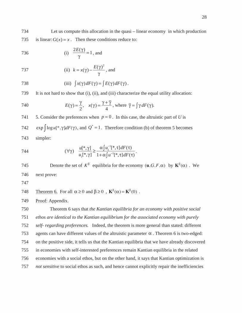
Let us compute this allocation in the quasi – linear economy in which production 734
is linear: . Then these conditions reduce to: 735
(i) , and 736
(ii) , and 737
(iii) . 738
It is not hard to show that (i), (ii), and (iii) characterize the equal utility allocation: 739
, where 740
5. Consider the preferences when . In this case, the altruistic part of U is 741
exp logu[*, ]dF( ) , and . Therefore condition (b) of theorem 5 becomes 742
simpler:743
.744
Denote the set of K equilibria for the economy (u,G,F, ) by K ( ) . We 745
next prove: 746
747
Theorem 6. For all 0 and 0 , K ( ) = K (0) . 748
Proof: Appendix. 749
Theorem 6 says that the Kantian equilibria for an economy with positive social 750
ethos are identical to the Kantian equilibrium for the associated economy with purely 751
self- regarding preferences. Indeed, the theorem is more general than stated: different 752
agents can have different values of the altruistic parameter . Theorem 6 is two-edged: 753
on the positive side, it tells us that the Kantian equilibria that we have already discovered 754
in economies with self-interested preferences remain Kantian equilibria in the related 755
economies with a social ethos, but on the other hand, it says that Kantian optimization is 756
not sensitive to social ethos as such, and hence cannot explicitly repair the inefficiencies 757
G(x) = x
2E( )= 1
k = x( ) E( )2
x( )dF( ) = E( )dF( )
E( ) =2
, x( ) = +
4= dF( ).
p = 0
Q*= 1
( ) u[*, ]u1[*, ]
u11[*, ]dF( )
1+ u 1[*, ]dF( )

29
which may come into being because of the consumption externalities concomitant with 758
other-regarding preferences. 759
We do, however, have one instrument -- namely, -- which may help achieve 760
Pareto efficient allocations when . Indeed, consider the family of quasi-linear 761
economies, where, for some fixed 762
. (6.6) 763
For these economies we can always choose a value so that the equilibrium w.r.t. 764
the allocation rule X is efficient for economies with any value of : that is to say, the765
(K ,X ) allocation maximizes social welfare (and so is in ). 766
Theorem 7 Let , some . Let G be any concave production 767
function. Define by the equation where . Then768
for this economy : 769
(a) An allocation is PE(0) iff . 770
(b) Define . The allocation w.r.t. the allocation rule X is in 771
.772
(c) As from below, the maximum value of for which the (K ,X ) allocation 773
is in approaches infinity. 774
Proof: Appendix. 775
The reader is entitled to ask: What happens for ? The answer is that, in 776
the (K ,X ) allocation, some utilities become negative, so social welfare for the CES 777
family of functions is undefined, and so all-encompassing utility U is undefined. 778
779
B. Taxation in private-ownership economies 780
The equilibria for the allocation rules X are not implementable with 781
markets in any obvious way. This is most easily seen by noting that the proportional rule 782
> 0
>1:
u (x, E) = x E
K
PE( )
u (x, E) = x E >1
E E = G (E)1/( 1) 1/( 1) dF( )
E( ) = 1/( 1)G (E)1/( 1)
( ) = G(E)G (E)
E K
PE( )
( )
PE( )
> ( )
K

30
is not so implementable. According the second theorem of welfare economics, there is 783
some division of shares in the firm which operates the technology G which would 784
implement these rules in Walrasian equilibrium in continuum economies, but to compute 785
those shares, one would have to know the preferences of the agents. The advantage of 786
the Kantian approach is that the Kantian allocations are decentralizable in the sense that 787
agents need only know the production function G , average effort , and their own 788
preferences, to compute the deviation they would like (everybody) to make. 789
Nevertheless, one would like Kantian optimization to be useful in market 790
economies as well. For the linear economies, we have a hopeful result – namely, 791
Theorem 2. Before stating it, let us define the allocation rules associated with linear 792
taxation. Define the affine tax allocation rule X[t ] for linear economies with production 793
function by: 794
X[t ](E1,...,En ) = (1 t)aE + t aE
S
n . (6.7) 795
Theorem 8 796
A. For any , the equilibria for the linear tax rule X[t ] is Pareto efficient on797
.798
B. The only allocation rules which are efficiently implementable in on are of 799
the form X (E1,...,En ) = X[t ](E1,...,En )+ k (E1,...,En ) for some where: 800
(i) for all E +n k (E) = 0 , 801
(ii) for all (j,E) X (E) 0 , and 802
(iii) for all , for all E +n , k (E) E = 0 . 803
804
Proof: Part A is simply Theorem 2; part B is proved in the appendix. 805
By virtue of Part A of the above theorem, and Theorem 6, in a society with other-806
regarding preferences and linear production, citizens could choose a high tax rate to 807
redistribute income substantially, without sacrificing allocative efficiency, thereby 808
addressing the positive externality due to their concern for others. Part B of the theorem 809
is analogous to part C of Theorem 3.810
E
G(x) = ax
t [0,1] K +
L0, fin
K + L
0, fin
t [0,1]
31
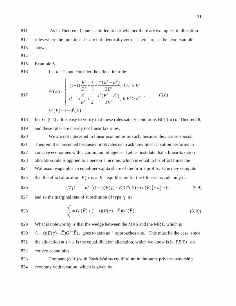
As in Theorem 3, one is entitled to ask whether there are examples of allocation 811
rules where the functions are not identically zero. There are, as the next example 812
shows.813
814
Example 5.815
Let n = 2, and consider the allocation rule: 816
, (6.8) 817
for . It is easy to verify that these rules satisfy conditions B(i)-(iii) of Theorem 8, 818
and these rules are clearly not linear tax rules.819
We are not interested in linear economies as such, because they are so special. 820
Theorem 8 is presented because it motivates us to ask how linear taxation performs in 821
concave economies with a continuum of agents. Let us postulate that a linear-taxation 822
allocation rule is applied to a person’s income, which is equal to his effort times the 823
Walrasian wage plus an equal-per-capita share of the firm’s profits. One may compute 824
that the effort allocation is a equilibrium for the t-linear tax rule only if: 825
( ) , (6.9) 826
and so the marginal rate of substitution of type is: 827
. (6.10) 828
What is noteworthy is that the wedge between the MRS and the MRT, which is 829
, goes to zero as approaches one. This must be the case, since 830
the allocation at is the equal-division allocation, which we know is in PE(0) on 831
convex economies.832
Compare (6.10) with Nash-Walras equilibrium in the same private-ownership 833
economy with taxation, which is given by: 834
k j
1(E) =(1 t) E1
ES + t2+ t2(E1 E2 )
2ES , if E1 E2
(1 t) E1
ES + t2
t2(E2 E1)2ES , if E1 E2
2(E) = 1 1(E)
t (0,1)
E( ) K +
u1 (1 t)(E( ) E)G (E)+G (E)( ) + u2 = 0
u2
u1
= G (E)+ (1 t)(E( ) E)G (E)
(1 t)(E( ) E)G (E) t
t = 1

32
. (6.11) 835
Here, the wedge between the MRS and the MRT is which becomes equal to the 836
whole MRT as t goes to one. If there is positive social ethos, citizens might well wish to 837
redistribute market incomes via taxation. Under Nash optimization, it becomes 838
increasingly costly to do so (as taxes increase), while with optimization, equation 839
(6.10) suggests it becomes decreasingly costly to do so, in terms of deadweight loss. 840
841
7. Existence and dynamics 842
The existence of proportional solutions, which are the equilibria of convex 843
economies (u,G,n) was proved in Roemer and Silvestre (1993). Here, we provide 844
conditions under which K equilibria exist, with respect to the allocation rules described 845
in Theorem 3. 846
847
Theorem 9. . Let (u,G,n) be a finite economy where the component functions of u are 848
strictly concave. 849
A. If for all , , 2u
x E0 then a strictly positive equilibrium w.r.t. the equal-850
division allocation rule X exists . 851
B. Let . If for all , u is quasi-linear, then a strictly positive K equilibrium 852
w.r.t. the allocation rule X exists. 853
Proof: Appendix. 854
The premises of this theorem can surely be weakened11.855
We turn briefly to dynamics. There will not be robust dynamics for Kantian 856
equilibrium, as there are not for Nash equilibrium. There is, however, a simple dynamic 857
mechanism that will, in well-behaved cases, converge to a Kantian equilibrium from any 858
initial effort vector. The mechanism is based on the mapping defined in the proof of 859
Theorem 9. Informally, the dynamics are as follows. Beginning at an arbitrary vector of 860
11 As with Nash equilibria, there is no guarantee that Kantian equilibria are unique.
u2
u1
= (1 t)G (E)
tG (E)
K +
K ×
K +
0 <
33
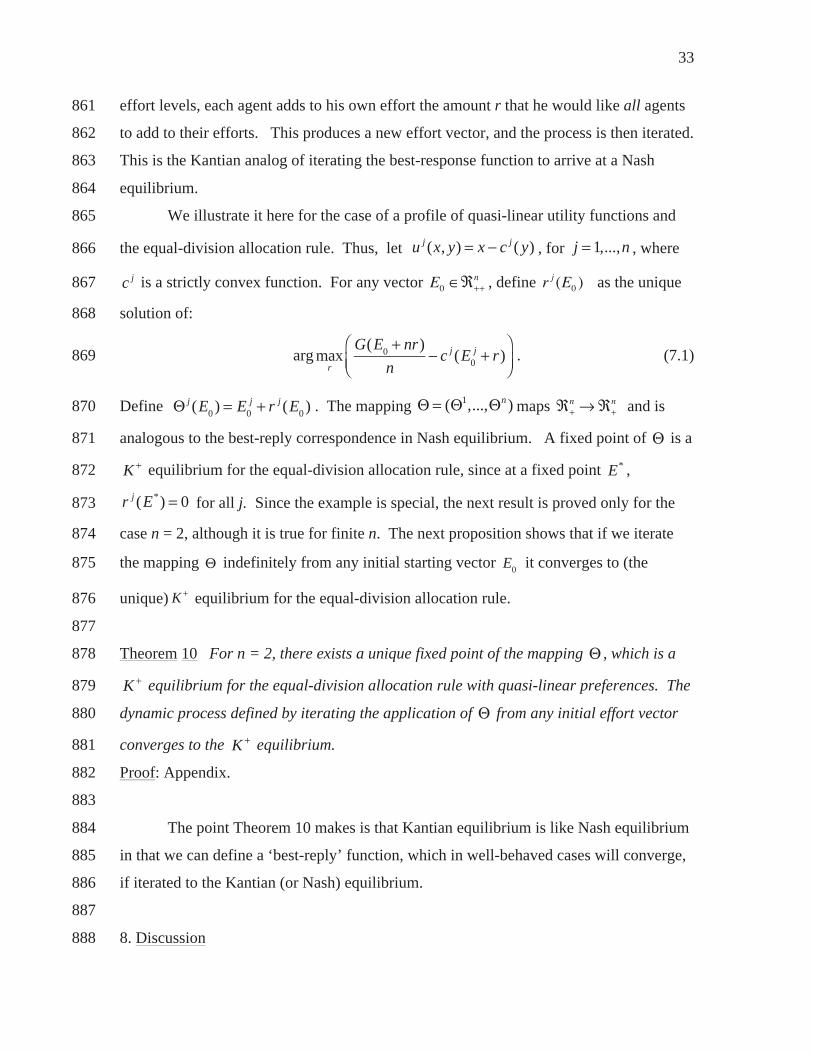
effort levels, each agent adds to his own effort the amount r that he would like all agents861
to add to their efforts. This produces a new effort vector, and the process is then iterated.862
This is the Kantian analog of iterating the best-response function to arrive at a Nash 863
equilibrium.864
We illustrate it here for the case of a profile of quasi-linear utility functions and 865
the equal-division allocation rule. Thus, let , for , where 866
is a strictly convex function. For any vector E0 ++n , define r j (E0 ) as the unique 867
solution of: 868
arg . (7.1) 869
Define . The mapping maps +n
+n and is870
analogous to the best-reply correspondence in Nash equilibrium. A fixed point of is a 871
equilibrium for the equal-division allocation rule, since at a fixed point , 872
for all j. Since the example is special, the next result is proved only for the 873
case n = 2, although it is true for finite n. The next proposition shows that if we iterate 874
the mapping indefinitely from any initial starting vector it converges to (the 875
unique) equilibrium for the equal-division allocation rule. 876
877
Theorem 10 For n = 2, there exists a unique fixed point of the mapping , which is a 878
equilibrium for the equal-division allocation rule with quasi-linear preferences. The 879
dynamic process defined by iterating the application of from any initial effort vector 880
converges to the equilibrium.881
Proof: Appendix.882
883
The point Theorem 10 makes is that Kantian equilibrium is like Nash equilibrium 884
in that we can define a ‘best-reply’ function, which in well-behaved cases will converge, 885
if iterated to the Kantian (or Nash) equilibrium. 886
887
8. Discussion 888
u j (x, y) = x c j ( y) j = 1,...,n
c j
maxr
G(E0 + nr)n
c j (E0j + r)
j (E0 ) = E0j + r j (E0 ) = ( 1,..., n )
K + E*
r j (E*) = 0
E0
K +
K +
K +
34
My analysis has been positive rather than normative. I have argued that if agents 889
optimize in the Kantian way, then certain allocation rules will produce Pareto efficient 890
allocations, while Nash optimization will not. While the analysis is positive, Kantian 891
optimization, if people follow it, is motivated by a moral attitude or social norm: each 892
must think that he should take an action if and only if he would advocate that all others 893
take a similar action. Optimization protocols differ from preferences: thus, optimizing 894
according to the Kantian protocol implies nothing about whether one’s preferences are 895
other-regarding or self-interested – rather, it has to do with cooperation. You and I may 896
cooperate, to our mutual benefit, whether or not we care about each other. Is it plausible 897
to think that there are (or could be) societies where individuals do (or would) optimize in 898
the Kantian manner?899
Certainly parents try to teach Kantian behavior to their children, at least in some 900
contexts. “Don’t throw that candy wrapper on the ground: How would you feel if 901
everyone did so?” The golden rule (“Do unto others as you would have them do unto 902
you” ) is a special case of Kantian ethics. (And wishful thinking [“if I do X, then all 903
those who are similarly situated to me will do X”], although a predictive claim, rather 904
than an ethical one, will also induce Kantian equilibrium – if all think that way.) This 905
may explain why people vote in large elections, and make charitable contributions. So 906
there is some reason to believe that Kantian equilibria are accessible to human societies. 907
Consider the relationship between the theoretical concept of Nash equilibrium and 908
the empirical evidence that agents play the Nash equilibrium in certain social situations 909
that can be modeled as games. We do not claim that agents are consciously computing 910
the Nash equilibrium of the game: rather, we believe there is some process by which 911
players discover the Nash equilibrium, and once it is discovered, it is stable, given 912
autarkic reasoning. We now know there are many experimental situations in which 913
players in a game do not play (what we think is) the Nash equilibrium. Conventionally, 914
this ‘deviant’ behavior has been rationalized by proposing that players have different 915
payoff functions from the ones that the experimenter is trying to induce in them, or that 916
they are adopting behavior that is Nash in repeated games generated by iterating the one-917
shot game under consideration. Another possibility, however, is that players in these 918
games are playing some kind of Kantian equilibrium. In Roemer (2010), I showed that if, 919

35
in the prisoners’ dilemma game, agents play mixed strategies on the two pure strategies 920
of {Cooperate, Defect}, then all multiplicative Kantian equilibria entail both players’ 921
cooperating with probability at least one-half (i.e., no matter how great is the payoff to 922
defecting). It can also be shown that, in a stochastic dictator game, where the dictator is 923
chosen randomly at stage 1 and allocates the pie between herself and the other player in 924
stage 2, the unique equilibrium is that each player gives one-half the pie to the other 925
player, if he is chosen.926
The non-experimental (i.e., real-world) counterpart, as I have said in the 927
introduction, may be the games that the societies that Elinor Ostrom has studied are 928
playing. If these games can be modeled as ‘fisher’ economies, with common ownership 929
of a resource whose use displays congestion externalities, and if, as Ostrom contends, 930
these societies figure out how to engender efficient allocations of labor applied to the 931
common resource, then they are discovering the multiplicative Kantian equilibrium of the 932
game. Perhaps Kantian reasoning helps to maintain the equilibrium: optimizing behavior 933
may be cooperative and not autarkic. Ostrom explains the maintenance of the efficient 934
labor allocation by invoking the community’s use of sanctions and punishments, but that 935
may not be the entire story: it may be that many fishers are thinking in the Kantian 936
manner, and that punishments and monitoring are needed only to control a minority who 937
are Nash optimizers. I am proposing that an ethic may have evolved, in these societies, 938
in which the fisher says to himself, “I would like to increase my fishing time by 5% a 939
week, but I have a right to do so only if all others could similarly increase their fishing 940
times, and that I would not like. ” Armed only with the theory of Nash equilibrium, one 941
naturally thinks that these Pareto efficient solutions to the tragedy of the commons 942
require punishments to keep everyone in line.943
As I noted earlier, Kantian ethics, and therefore the behavior they induce, require 944
less selflessness than another kind of ethic: putting oneself in the shoes of others.945
Consider charity. “I should give to the unfortunate, because I could have been that 946
unfortunate soul – indeed, there but for the grace of God go I. ” The Kantian ethic says, 947
in contrast: “I will give to the unfortunate an amount which I would like all others who 948
are similarly situated to me to give.” Assuming that there is a social ethos (that is, ) 949
K ×
> 0

36
this kind of reasoning may induce substantial charity – or, in the political case, fiscal 950
redistribution. Cooperation is the active behavior rather than empathy. 951
To the extent that human societies have prospered by exploiting the ability of 952
individuals of members of our species to cooperate with each other, it is perhaps likely 953
that Kantian reasoning is a cultural adaptation, selected by evolution ( the classic 954
reference is Boyd and Richerson [1985]). Because we have shown that Kantian behavior 955
can resolve, in many cases, the inefficiency of autarkic behavior, cultures which discover 956
it, and attempt to induce that behavior in their members, will thrive relative to others.957
Group selection may produce Kantian optimization as a meme. Imagine, for example, a 958
time when there were many societies of fishers. Suppose that in a small number of these 959
societies, a clever priest or shaman proposed that fishers optimize using the multiplicative 960
Kantian protocol. These societies, given the proportional allocation rule, will achieve 961
Pareto efficient allocations. If utility measures fitness, these societies will prosper while 962
those using the Nash protocol will not. The meme of Kantian optimization could 963
spread12.964
One can rightfully ask whether it is utopian to suppose that the allocation rules 965
studied here can be used in large economies13. Even if the allocation rules of Theorem 3 966
are not employed, one may ask what happens if agents in a private-ownership economy 967
with markets optimize by choosing their effort supplies in the Kantian manner. I have 968
done some simulations of the affine-tax allocation rules where the market allocation is 969
Walrasian, and the production function is strictly concave14. We do not get full Pareto 970
12 For some preliminary evolutionary analysis of Kantian behavior, see Curry and Roemer (2012). 13 An interesting recent example is the behavior of the small island nation of Mauritius with regard to global warming, which will affect it severely, through rising sea levels.Mauritius has undertaken serious steps to reduce its carbon footprint, although this will have negligible effect on its own situation (namely, the sea level). It is behaving as a Kantian optimizer, taking the action it would like all other nations to take. Kantian optimization, in this case, is an attempt to set a moral example. See the Maurice Ile Durable website (http://www.gov.mu/portal/sites/mid/index.html). We can think of many other examples where individuals have attempted to induce cooperative behavior in others by their moral example. 14 Available from the author.
37
efficiency, but the results are better when agents optimize in the additive Kantian way 971
than when they are Nash optimizers.972
One of the motivations I gave for studying Kantian optimization was to resolve 973
the inefficiencies in economies with a social ethos, due to the consumption externalities 974
that they entail. One might think that, if a society is altruistic in the sense of possessing 975
a social ethos, then it is more likely that its members would behave in a cooperative 976
fashion. The behavior upon which I have focused in this article is optimizing behavior.977
I have not argued, however, that there is a link between a community’s possessing a 978
social ethos and its members’ learning and employing Kantian optimization, although I 979
suspect that there is. I leave the reader with this question.980
981

38
982
989990991992993994995996997998999
100010011002100310041005
Figure 1. Illustration of Kantian counterfactual rays for n = 2. 10061007
K+K+K
N1
N2

39
References1008
Alger, I. and J.W. Weibull, 2012. “Homo Moralis: Preference evolution under 1009
incomplete information and assortative matching,”1010
http://pzp.hhs.se/media/5245/homomoralis120206_wp.pdf1011
Arneson, R. 1989. “Equality and equality of opportunity for welfare,” Phil. Stud.1012
56, 77-93 1013
Bowles, S. and H. Gintis, 2011. A cooperative species: Human reciprocity and its 1014
evolution, Princeton: Princeton University Press 1015
Boyd, R. and P. Richerson, 1985. Culture and the evolutionary process,Chicago:1016
University of Chicago Press 1017
Brekke, K.A., S. Kverndokk, and K. Nyborg, 2003. “An economic model of 1018
moral motivation,” J. Public Econ. 87, 1967-1983 1019
Cohen, G.A. 1989. “On the currency of egalitarian justice,” Ethics 99, 906-944 1020
Cohen, G.A. 2009. Why not socialism? Princeton: Princeton University Press 1021
Curry, P. and J. Roemer, 2012. “Evolutionary stability of Kantian optimization,” 1022
Review of Public Economics (Hacienda Publica Espanola), 200-(I/2012), 131-148 1023
Dufwenberg, M., P. Heidhues, G. Kirchsteiger, F. Riedel, and J. Sobel, 2011. 1024
“Other regarding preferences and general equilibrium,” Rev. Econ. Stud. 78, 613-639 1025
Dworkin, R. 1981. “What is equality? Part 2: Equality of resources,” Phil. & Pub. 1026
Affairs 10, 283-345 1027
Fleurbaey, M. 2008. Fairness, responsibility, and welfare, Oxford University 1028
Press1029
Harsanyi, J. 1977. Rational behavior and bargaining equilibrium in games and 1030
social situations, Cambridge University Press 1031
Henrich, N. and J. Henrich, 2007. Why humans cooperate: A cultural and 1032
evolutionary explanation, Oxford: Oxford University Press 1033
Olson, M. 1965. The logic of collective action, Cambridge MA: Harvard 1034
University Press 1035
Ostrom, E. 1990. Governing the commons: The evolution of institutions for 1036
collective action, Cambridge: Cambridge University Press 1037

40
Ostrom, E. and R. Gardner, 1993. “Coping with asymmetries in the commons: 1038
Self-governing irrigation systems can work,” J. Econ. Perspectives 7, 93-112 1039
Rabin, M. 2006. “The experimental study of social preferences,”Social Research1040
73, 405-428 1041
Rawls, J. 1971. A theory of justice, Cambridge, MA: Harvard University Press 1042
Roemer, J. 1996. Theories of distributive justice, Cambridge, MA: Harvard 1043
University Press 1044
Roemer, J. 1998. Equality of opportunity, Cambridge, MA: Harvard University 1045
Press1046
Roemer, J. 2010. “Kantian equilibrium,” Scandinavian J. Econ. 112, 1-24 1047
Roemer, J. and J. Silvestre, 1993. “The proportional solution for economies with 1048
both private and public ownership,” J. Econ. Theory 59, 426-444 1049
Scheve, K. and D. Stasavage, 2012. “Democracy, war and wealth: Lessons from 1050
two centuries of inheritance taxation,” Amer. Pol. Sci. Rev. 106, 81-102 1051
1052
1053
“Appendix: proofs of theorems”1054 1055
Proof of Theorem 3. 1056
The proof of part A simply mimics the proof of Theorem 1. We prove part B. 1057
1. Consider the Kantian variation (x,r) = rx + (r 1) , and any allocation rule 1058{ j , j = 1,...,n}, defined for a finite economy with n agents. The condition that must hold 1059for a rule to be efficiently implemented on E in K equilibrium is the FOC: 1060
1061
( j)j (E) (E + )G(ES )+ j (E)G (ES )(ES + n )
E j += G (ES ) , (A.1) 1062
1063which is the statement that that at a K equilibrium E = (E1,..., En ) , the marginal rate of 1064
substitution between effort and income for each agent is equal to the marginal rate of 1065
transformation. Recall that ES E j , j is the gradient of the function j with 1066

41
respect to its n arguments, E + is the vector whose jth component is E j + , and 1067
j (E) (E + ) is the scalar product of two n vectors. (A.1) can be written as: 10681069
( j (E) (E + )E j +
) G(ES )G (ES )
+ j (E) (ES + n )E j +
= 1. (A.2) 1070
2. We now argue that (A.2) must hold as a set of partial differential equations on ++n .1071
For let E ++n be any vector. Fix a production function G. We can always construct n1072
utility functions whose marginal rates of substitution at the points ( j (E)G(ES ), E j ) are 1073
exactly given by the value of the left-hand side of equation (A.1). For the economy thus 1074
defined, E is indeed a K equilibrium. This demonstrates the claim. 1075
3. Continue to fix a vector E ++n . Define ri
j =Ei +E j +
for i = 1,...,n and notice that 1076
(E j ,rij ) = Ei . Consider the ray gotten by varying x, defined in the text:1077
M (E) = ( (x,r1j ), (x,r2
j ),..., (x,rnj )) . Note that when x = E j , this picks out the 1078
vector E. We will reduce the system (A.2) of PDEs to ordinary differential equations on 1079
M (E) .1080
1081Define j (x) = j ( (x,r1
j ),..., (x,rnj )) . Note that : 1082
( j ) (x) = j ( (x,r j )) r j (A.3) 1083
where (x,r) is the generic vector in the ray, and r j = (r1j ,...,rn
j ) .1084
Define j (x) = G( (x,rij )) and note that: 1085
( j ) (x) = G ( (x,rij )) ri
j . (A.4) 1086
It follows that we may write (A.2) restricted to the ray M (E) as: 1087
( j ) (x)r S , jj (x)
( j ) (x)+ j (x)r S , j = 1, (A.5) 1088

42
where r S , j rij
i.1089
4. (A.5) is a first-order ODE. A particular solution is given by the constant function: 1090j (x) = 1
r S , j , (A.6) 1091
and the general solution to its homogeneous variant is: 1092
ˆ j (x) =k j ( M (E))
j (x), (A.7) 1093
where k j a constant that depends on the ray M (E) . Therefore the general solution of 1094
(A.5) is1095
j (x) = 1r S , j +
k j ( M (E))j (x)
. (A.8) 1096
Now, evaluating this equation at x = E j gives:1097
j (E j ) = j (E) = 1r S , j +
k j ( M (E))G(ES )
= E j +(Ei + )
+k j ( M (E))
G(ES ). (A.9) 1098
Since the n shares in (A.8) sum to one, (A.8) tells us that we must have k j ( M (E))j
= 0 .1099
5. Finally, we verify that the allocation rules defined in (A.9) satisfy the PDEs (A.2). If 1100
k j (M (E)) = 0 for all j, then j (E) = 1
rS, j , and it is proved in part A that this rule 1101
satisfies (A.2). So we assume that k j (M (E)) 0 for some j. To prove (A.2) holds,1102
we must show that : 1103
k j (E)G(ES )
(E + )E j +
) G(ES )G (ES )
+ k j (E)G(ES )
(ES + n )E j +
= 0. (A2a)1104
Recalling that by definition k j (E) (E + ) = 0 , because k j (E) is constant on M (E) ,1105
(A2a) is checked by computation. 1106
6. To prove part B, return to equation (A.8) which holds on the ray M (E) . For = 01107
(i.e., K × equilibrium), the ray M0(E) ={(r1j x,...,rn
jx) | x 0}. Hence, as x approaches 1108
zero j (x) approaches zero. If, for some j, k j ( M0(E)) 0 , then for sufficiently small x,1109
j (x) would violate the constraint that it lie in [0,1] . Hence, for the case when = 01110
43
(and only for that case) we may conclude that the constants k j are identically zero, and 1111
the claim of part B follows.1112
7. Part D is immediately verified by simple algebra.1113
1114
Proof of Theorem 4: 1115
1. An interior allocation E is Nash implementable on the class of finite convex 1116
economies for the allocation rule if and only if 1117
j u1j (
j (E)E j
G(ES )+ j (E)G (ES ))+ u2j = 0 (A.10) 1118
Therefore is efficiently implementable iff: 1119
j 1= j (E)+ G(ES )G (ES )
j (E)E j
. (A.11) 1120
2. Indeed, (A.11) must hold for the entire positive orthant ++n , for given any positive 1121
vector E, we can construct n concave utility functions such that (A.10) holds at E.11221123
3. For fixed E, define j (x) = j (E1, E2 ,..., E j 1,x, E j+1,..., En ) and 1124j (x) = G(x + ES E j ) . Then (A.11) gives us the differential equation: 1125
1126
1= j (x)+j (x)
( j ) (x)( j ) (x) , (A.12) 1127
which must hold on ++ .11284. But (A.12) implies that1129
( j ) (x)1 j (x)
= ( j ) (x)j (x)
(A.13) 1130
which implies that j (x)(1 j (x)) = k j and therefore j (x) = 1 k j (E j )j (x)
where 1131
the constant k j may depend on the ray (E1,.., E j 1,x, E j+1,.., En ) on which j is defined. 1132.11335. In turn, this last equation says that on the ray (E1,..., E j 1,x, E j+1,..., En ) we have: 1134
j (E1,..., E j 1,x, E j+1,..., En )G(x + ES E j ) = G(x + ES E j ) k j (E j ) , (A.14) 1135
which says that ‘every agent receives his entire marginal product’ on this space. To be 1136
precise:1137
44
1138
( x, y > 0)( j (E1,..., E j 1,x, E j+1,..., En )G(x + ES E j )
j (E1,..., E j 1, y, E j+1,..., En )G( y + ES E j ) =
G(x + ES E j ) G( y + ES E j ))
1139
1140
(A.15) 1141Now let y = 0 and x = E j and let z j =
j (E1,..., E j 1,0, E j+1,..., En )G(ES E j ) . Then 1142
(A.15) says that: 1143
( j)( j (E)G(ES ) z j = G(ES ) G(ES E j )) . (A.16) 1144
6. Adding up the equations in (A.16) over j, and using the fact that z j 0 , we have: 1145
G(ES ) nG(ES ) G(ES E j ) (A.17) 1146
or:1147
G(ES ) 1n 1
G(ES E j ) . (A.18) 1148
1149
7. Now note that 1n 1
(ES E j ) = ES . Therefore (A.18) can be written: 1150
G( 1n 1
(ES E j ))1
n 1G(ES E j ) , (A.19) 1151
which is impossible for any strictly concave G. This proves part A of the theorem. 1152
8. The proof of part B is well-known: for part B just says that Nash behavior, taking 1153
prices as given, at the Walrasian allocation rule, induces Pareto efficiency. 1154
115511561157
Proof of Theorem 5: 1158
Consider the program: 1159
45
maxK ,h(),q()
u (x*( )+ h( ), E*( )+ q( )D
)dF( )+ F(D)K
subject tou (x*( )+ h( ), E*( )+ q( ))+ K u (x*( ), E*( ))+ K *
x*( )+ h( ) 0E*( )+ q( ) 0
K u (x*( )+ h( ), E*( )+ q( )) p dF( )( )1/ p
G( (E*( )+ q( ))dF( )) (x*( )+ h( ))dF( )
1160
1161
where D is any set of types of positive measure. Suppose the solution to this program is 1162
. (K* is the value of the social-welfare function – given in the K1163
constraint in the program -- when h = q = 0 .) Then (x*( ), E*( )) is a Pareto efficient1164
allocation. Since we are studying strictly positive allocations, the second and third sets of 1165
constraints at the proposed optimal solution will be slack. 1166
We will show that conditions (a) and (b) of the proposition characterize the * 1167
allocations for which this statement is true. Let be any feasible triple in the 1168
above program, for a fixed positive allocation (x*, E*) . Let . Then define 1169
the Lagrange function: 1170
1171
( ) = u (x*( )+ h( ), E*( )+ q( )D
)dF( )+ F(D)(K * + K )+
G( (E*( )+ q(t))dF( ) (x*( )+ h( ))dF( )( ) + u (x*( )+ h( ), E*( )+ q( )) p dF( )1/ p
K * + K )( ) + B( )(u(x*( )+ h( ), E*( )+ q( ), )+ K u(x*( ), E*( ), ))dF( ).
1172
1173
1174
Suppose there is non-negative function B( ) and non-negative numbers for which 1175
the function is maximized at zero. Note is the value of the objective of the 1176
above program, when and , and equals the value of the 1177
objective at plus some non-negative terms. The claim will then follow. Since 1178
h* 0, q* 0, K = K *
(h,q, K )
K = K K *
( , )
(0)
h* 0 q* K = K * (1)
(h,q, K )

46
is a concave function, it suffices to produce an allocation (x*, E*) for which non-1179
negative exist such that . 1180
Compute the derivative of at zero: 1181
1182
(0) = u1[*, ]h( )+ u2[*, ]q( )dF( )( )D
+ F(D) K +
G ( E*( )dF( )) q( )dF( ) h( )dF( )( ) +
p(Q*)(1 p)/ p p u[*, ]p 1 u1[*, ]h( )+ u2[*, ]q( )( )dF( )
K + B( ) u1[*, ]h( )+ u2[*, ]q( )+ K( )dF( ).
1183
1184
We now gather together the coefficients of K ,h, and q in the above expression 1185
and set them equal to zero: 1186
1187
Coefficient of K : F(D)+ B( )dF( ) = 0 (A.9) 1188
Coefficient of h( ) : u1[*, ]1D + (Q*)(1 p)/ p u[*, ]p 1u1[*, ]+ B( )u1[*, ]= 0 , (A.10) 1189
Coefficient of q( ) : u2[*, ]1D + G (E)+ (Q*)(1 p)/ p u[*, ]p 1u2[*, ]+ B( )u2[*, ] = 0 , (A.11)1190
where and E = E*( )dF( ) .1191
By setting all these coefficients equal to zero, and solving for the Lagrange 1192
multipliers, we will discover the characterization of the allocation . Note that, 1193
at an interior Pareto efficient solution, we must have: 1194
u2[*, ]u1[*, ]
= G (E) ,1195
for this is the statement that the marginal rate of substitution for each type between labor 1196
and output is equal to the marginal rate of transformation between labor and output.1197
Therefore write: 1198
u1[*, ]+ u2[*, ]= u1[*, ] 1+u2[*, ]u1[*, ]
= u1[*, ] 1 G (E)( ) . (A.12) 1199
(B, , ) (0) = 0
1D ( ) =1, if D0, if D
(x*(), E*())
47
Now add together the equations for the coefficients of q( ) and h( ) , divide this new 1200
equation by 1 G (E) , use equation (A.12), and the result is exactly the equation (A.11). 1201
Therefore, eqn. (A.12) has enabled us to eliminate equation (A.11): if we can produce 1202
non-negative values (B( ), , ) satisfying (A.9) and (A.10), we are done. 1203
Solve eqn. (A.10) for B( ) :1204
B( ) =u1[*, ]1D u1[*, ] (Q*)(1 p)/ p u[*, ]p 1
u1[*, ] . (A.13) 1205
From eqn. (A.9), we have = F(D)+ B( )dF( ) , and substituting the expression 1206
for B( ) into this equation, we integrate and solve for :1207
=u1[*, ] 1 dF( )
1+ (Q*)(1 p)/ p u[*, ]p 1 dF( ) (A.14). 1208
1209
Eqn. (A.13) says that B( ) is non-negative if and only if1210
u1[*, ](1D + (Q*)(1 p)/ p u[*, ]p 1) ; (A.15) 1211
substituting the expression for from (A.14) into (A.15) yields an inequality in which, 1212
by rearranging terms, can be written as: 1213
1 u1[*, ](Q*)(1 p)/ p u[*, ]p 1 u1[*, ] 1 dF( )1+ (Q*)(1 p)/ p u[*, ][ 1 dF( )
u1[*, ] . (A.16) 1214
In sum, we can find non-negative Lagrange multipliers iff we can produce a non-negative 1215
number such that (A.16) is true for all . This can be done iff: 1216
1u1[*, ]
(Q*)(1 p)/ p u[*, ]p 1 u1[*, ] 1 dF( )1+ (Q*)(1 p)/ p u[*, ]p 1 dF( )
,1217
proving the theorem.1218
1219
Proof of Theorem 6. 1220
We prove the generalization of the theorem stated in the text. We prove the result 1221
for K × equilibrium for simplicity’s sake, although the proof for K equilibrium is the 1222
same. Also for simplicity’s sake, we use the social-welfare function of (1.1). 1223
48
1. For the allocation rule , an allocation E is a K × equilibrium iff: 1224
ddr
|r=1 u ( (rE)G(rE),rE( ))+ exp log(u ( (rE)G(rE),rE( ))dF( )( ) = 0 , (A.17) 1225
where we assume that the altruism parameters { } are non-negative. Expand this 1226
derivative, writing it as: 1227
( ) D (E)+ exp log(u ( (E)G(E), E( ))dF( ) D (E)u
dF( ) = 0, (A.18) 1228
where D (E) = ddr r=1
u ( (rE)G(rE),rE( )) .1229
2. Now (A.18) says that : 1230( )(D (E) = k)1231
where k is a constant (independent of ). Therefore we can substitute k for D (E)1232
on the r.h.s. of eqn. (A.18), and re-write that equation as: 1233
k km = 0 , (A. 19) 1234
where m is a positive constant. If = 0 , we have from (A.18) that D (E) = 0 . If 1235
0 , it follows from (A.19) that k = 0 . But this means that for all , D (E) = 0 ,1236
which is exactly the condition that E is a Kantian equilibrium for the economy with 1237
= 0 .1238
1239
Proof of Theorem 7: 1240
1241
1. The effort allocation in part (a) maximizes the surplus, which is the condition for 1242
efficiency in the quasi-linear economy with = 0 .1243
2. Integrating the expression for E( ) , we have that the equation E = G (E)1/( 1) , 1244
characterizing E .1245
3. To prove claim (b), we show that the ( ) -Kantian1246
equilibrium produces equal utilities across . From Remark 4 stated after Theorem 3, 1247
this suffices to show that the allocation will be in PE( ) . We have: 1248

49
u[ , ]=1/( 1)G (E)1/( 1) +
G (E)1/( 1) +G(E)
/( 1)G (E) /( 1)
=
1/( 1) G (E)1/( 1)G(E)G (E)1/( 1) +
G (E) /( 1)
+ k (A.17) 1249
1250
where k is a constant independent of . Calculation shows that the value of that 1251
causes the coefficient of 1/( 1) in (A.17) to vanish is ( ) as defined in claim (b). It is 1252
easy to observe that ( ) > 0 by the concavity of G, and because >1. This proves 1253
claim (b). 1254
4. Claim (c) follows from analyzing the condition (b) of theorem 5, which for quasi-1255
linear economies is: 1256
( ) 1+ u[*, ] 1 dF( ) u[*, ] 1 ,1257
1258
as approaches ( ) from below. 1259
1260
Proof of Theorem 8: 1261
1. A simple calculation shows that if E is a K + equilibrium for an economy with a 1262
linear production function G(x) = ax w.r.t. any linear tax allocation rule [t ] , for t [0,1],1263
then the allocation is 0-Pareto efficient.1264
2. Now let E be a K + equilibrium w.r.t. any allocation rule on (u,G, F ,0) which is 1265
Pareto efficient on that economy. E is a K + equilibrium means: 1266
u1j ( j (E) 1)aES + j (E)an( ) + u2
j = 0 ,1267
and so Pareto efficiency means that: 1268
( j (E) 1)aES + j (E)an( ) = a ,1269
or:1270
( j (E) 1)ES + n j (E) = 1. (A.18) 1271

50
As has been argued in previous proofs, (A.18) must hold as a system of partial 1272
differential equations on ++n .1273
3. Define rij = Ei E j . Define j (x) = j (x + r1
j ,...,x + rnj ) . Note that 1274
( j ) (E j ) = ( j (E) 1) . Hence, on the ray M (E) ={(x + r1j ,...,x + rn
j )} , we may write 1275
the differential equation (A.18) as: 1276
( j ) (x)(nx + r j ,S )+ n j (x) = 1, (A.19) 1277
where r j ,S = rij
i. Since the linear tax rules satisfy (A.18) by step 1, it follows that a 1278
particular solution of (A.19) is j (x) = (1 t) xnx + r j ,S + t
n, for any t [0,1] . The 1279
general solution to the homogeneous variant of (A.19) is j (x) = k j
nx + r j ,S , where k j is 1280
a constant that may depend upon the ray M (E) . Therefore the general solution to 1281
(A.19) is: 1282
j (x) = (1 t) xnx + r j ,S + t
n+ k j
nx + r j ,S ,1283
where t may be chosen freely, and k j is as described. Translating back, this means that 1284
j (E) = [t ]j (E)+ k j (E)
ES1285
where we must have: 1286
(i) for all E, k j (E) = 01287
(ii) j (E) [0,1]1288
(iii) for all j and E, k j (E) 1 = 0 .1289
Statements (i) and (ii) are obvious requirements, while statement (iii) says that the 1290
functions k j are constant on the ray M (E) .1291
1292
Proof of Theorem 9: 1293
Part A 1294
1. Define the functions: 1295

51
r j (K , y) = maxr
u j (G(K + y + nr)n
, y + r) for (K , y) +2 .1296
These are single-valued functions, by strict concavity of u.1297
1298
The first-order condition defining rj is: 1299
u1j ( )G (K + y + nr)+ u2
j ( ) = 0 .1300
1301
2. Using the implicit function theorem, compute that the derivatives of r j w.r.t. its 1302
arguments are : 1303
drdK
=u1
jG + u11j G 2 + u12
j Gn(u1
jG + u11j (G )2 + 2G u12
j + u22j )
< 0.
1304
1305
The denominator of this fraction is negative by concavity of u and G, the the numerator is 1306
negative since u12j 0 , and hence dr
dK< 0 . And: 1307
drdy
=u22
j + (G )2u11j + (n+1)u12
j + u1jG
n(u22j + (G )2u11
j + 2G u12j + u1
jG )< 0 .1308
Likewise, drdy
< 0 .1309
3. Define y j by r j (0, y j ) = 0 . If all agents other than j are putting in zero effort, then y j1310
is the amount of effort for j at which he would not like to increase all efforts by any 1311
number. Now define K j = y j
i j. Next define z j by r j (K j , z j ) = 0 . z j is the 1312
amount of effort for j such that, if all other agents i are expending yi and he is expending 1313
z j , he would not like to add or subtract any amount from all efforts. 1314
4. We argue that z j < y j for all j. Just note that r j (K j , z j ) = 0 = r j (0, y j ) . Since 1315
K j > 0 , it follows that z j < y j , because the r j are decreasing functions. 1316
5. Hence we may define the non-degenerate rectangle ={E ++n | z E y}.1317
6. By applying the definition of r j (K , y) , note that we have the identity: 1318
52
r j (K + (n 1)b,a + b) = r j (K ,a) b .1319
7. We now define a function : +n
+n :1320
(E1,..., En ) = (E1 + r1( E 1, E1),..., En + r n( E n , En ))1321
where E j Ei
i j. is like the best-reply correspondence in Nash equilibrium. 1322
is single-valued and continuous, by the Berge maximum theorem.1323
We next show that ( ) . Let E = (E1,..., En ) . We must show: 1324
( j)(z j E j + r j ( E j , E j ) y j . (A.20) 1325
By step 6, we have1326
r j ( E j , E j ) ( y j E j ) = r j ( E j + (n 1)( y j E j ), y j ) 0 ,1327
where the inequality follows because r j is decreasing and r j (0, y j ) = 0 and 1328
E j + (n 1)( y j E j ) 0 . This proves the second inequality in (A. 20). 1329
Again by step 6, we have: 1330
r j ( E j , E j ) (z j E j ) = r j ( E j + (n 1)(z j E j ),z j ) 01331
where the inequality follows because r j is decreasing and E j + (n 1)(z j E j ) K j1332
(note that (n 1)(z j E j ) 0 ). This proves the first inequality in (A.20). 1333
8. Hence, the function satisfies all the premises of Brouwer’s Fixed Point Theorem, 1334
and hence possesses a fixed point. But a fixed point of is a vector E such that for all j,1335
r j ( E j , E j ) = 0 , which is precisely a K + equilibrium. (Note that the rectangle is in the 1336
strictly positive orthant, which implies that the equilibrium is strictly positive.) 1337
Part B 1338
9. The proof proceeds in the same fashion as above, except we now define the functions: 1339
r j (K , y) = argmaxr
u j ( ry + (r 1)+r(K + y)+ n (r 1)+ n
G(r(K + y)+ n(r 1) ,ry + (r 1)) .1340
Recall that y will be evaluated at E j and K at E j for a vector E.1341
The first-order condition defining the functions r j is: 1342
u1j G + u2
j = 0 ,1343
53
where u is evaluated at the point ( y +K + y + n
G(r(K + y)+ (r 1)n ),ry + (r 1) ) . We 1344
compute, using the implicit function theorem, that: 1345
dr j
dK=
(G u11j + u12
j ) y +K + y + n
G r j GK + y + n
+ r jG u1j
( y + )(G 2u11j + 2G u12
j + u22j )+ u1
jG (K + y + n ).1346
The denominator is negative by the concavity of u and G. Quasi-linearity implies that 1347
G u11j + u12
j = 0 and so the numerator is negative if r j > 0 . But note that we must have 1348
ry + (r 1) 0 , since efforts cannot be negative, and so r is restricted to the interval 1349
with lower bound ry +
> 0 , and so r j > 0 . Hencedr j
dK< 0 .1350
Compute that: 1351
dr j
dy=
u11j r jG 2 ( y + )
K + y + n+G G (K + (n 1) )
(K + y + n )2 + u12j r jG K + 2y + (n+1)
K + y + n+ K + y + (n 1)
(K + y + n )2 + r ju22j
( y + )(G 2u11j + 2G u12
j + u22j + u1 G (K + y + n )
1352
1353
The denominator is negative by concavity, and the numerator is negative since u12j = 0 ,1354
and so dr j
dy< 0 .1355
10. Hence the functions r j are decreasing, and the proof proceeds as before, from steps 1356
3 through 8.1357
1358
Proof of Theorem 10: 1359
The proof proceeds by showing that the mapping is a contraction mapping. It uses the 1360
following well-known mathematical result: 1361
Lemma Let be a norm on n and let
A be the associated sup norm on mappings1362
A : n n , defined by
A = supx =1
A(x) . Let J ( A) be the Jacobian matrix of A. If1363
J ( A) <1, then A is a contraction mapping.1364

54
If we can show that is a contraction mapping, then it possesses a unique fixed 1365
point, and the dynamic process induced by iterating the application of from any initial 1366
effort vector will converge to the fixed point. 1367
1. For n = 2 , the Jacobian of the map is 1+ r1
1 r21
r12 1+ r2
2, where 1368
rij (E1, E2 ) = r j
Ei (E1, E2 ) , assuming that these derivatives exist. Thus, the lemma 1369
requires that we show the norm of this matrix is less than unity. We take to be the 1370
Euclidean norm on 2 . We must show that: 1371
E = 11+ r1
1(E) r21(E)
r12(E) 1+ r2
2(E)E1
E2<1. (A.21) 1372
2. Assuming differentiability of c j , the function r j (E) is defined by the following first-1373
order condition: 1374
G (ES + 2r j (E)) = (c j ) (E j + r j (E)) , (A.22) 1375
which has a unique solution under standard assumptions. By the implicit function 1376
theorem, the derivatives of r j ( ) are given by: 1377
1378
G ( y j )(1+ 2rij (E)) = (c j ) (x j )( i
j + rij (E)) ,1379
where y j = G(ES + nr j (E)), x j = E j + r j (E) and ij =
1, if i = j0, if i j
; or 1380
rij (E) = i
j (c j ) (x j ) G ( y j )2G ( y j ) (c j ) (x j )
. (A.23) 1381
3. It follows from step 1 that the Jacobian of is given by: 1382
G ( y1)2G ( y1) (c1) (x1)
G ( y1)2G ( y1) (c1) (x1)
G ( y2 )2G ( y2 ) (c2 ) (x2 )
G ( y2 )2G ( y2 ) (c2 ) (x2 )
1383

55
and so, from step 1, we need only show that: 1384
(Q1(E1 E2 ))2 + (Q2(E1 E2 ))2 <1 (A. 24) 1385
where (E1, E2 ) = 1 and Q j = G ( y j )2G ( y j ) (c j ) (x j )
. Note that Q j < 12
. Therefore 1386
(A.24) reduces to showing that 12
(1 E1E2 ) <1, which is obviously true, proving the 1387
proposition.1388
1389
1390
1391
1392
13931394
1395