kapilthadani [email protected]€¦ · [email protected] research. outline 2...
TRANSCRIPT

2
Outline
◦ Language representation- Bag of words- Distributional hypothesis- Word embeddings: word2vec, GloVe- Beyond words: paragraph vector
◦ Recurrent neural networks- Backpropagation through time- Long short-term memory (LSTM)- Gated recurrent units (GRU)
◦ NLP scenarios- Classification- Tagging- Generation- Text-to-text
3
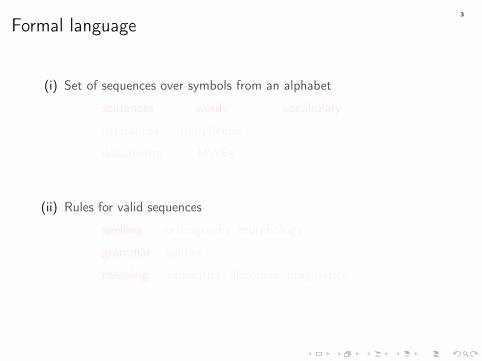
Formal language
(i) Set of sequences over symbols from an alphabet
sentences words vocabulary
utterances morphemes
documents MWEs...
...
(ii) Rules for valid sequences
spelling orthography, morphology
grammar syntax
meaning semantics, discourse, pragmatics, · · ·

3
Natural language
(i) Set of sequences over symbols from an alphabet
sentences words vocabulary
utterances morphemes
documents MWEs...
...
(ii) Rules for valid sequences
spelling orthography, morphology
grammar syntax
meaning semantics, discourse, pragmatics, · · ·

4
Sparse representations
Word: one-hot (1-of-V ) vectorsDocument: "bag of words"
Emphasize rare words with inverse documentfrequency (IDF)
Compare documents with cosine similarity
0...1...0
a
dog
zygote
|V |
+ Simple and interpretable− No notion of word order− No implicit semantics− Curse of dimensionality with large |V |

5
Sparse representations
Consider a neural network to read documents with:· at most T words· drawn from vocabulary V· into a hidden layer with H units
How many parameters in the input layer for:◦ Tweets?
◦ News stories?

5
Sparse representations
Consider a neural network to read documents with:· at most T words· drawn from vocabulary V· into a hidden layer with H units
How many parameters in the input layer for:◦ Tweets?T = 50, |V | = 100K, H = 100 → 0.5B
◦ News stories?

5
Sparse representations
Consider a neural network to read documents with:· at most T words· drawn from vocabulary V· into a hidden layer with H units
How many parameters in the input layer for:◦ Tweets?T = 50, |V | = 100K, H = 100 → 0.5B
◦ News stories?

5
Sparse representations
Consider a neural network to read documents with:· at most T words· drawn from vocabulary V· into a hidden layer with H units
How many parameters in the input layer for:◦ Tweets?T = 50, |V | = 100K, H = 100 → 0.5B
◦ News stories?T = 2000, |V | = 200K, H = 100→ 40B

6
Lexical semantics
dog

6
Lexical semantics
dog
mammal pet
hypernymy
poodle puppy
hyponymy
caninesynonymy
pack
holonymy
paw
meronymy

6
Lexical semantics
dog
mammal pet
hypernymy
poodle puppy
hyponymy
caninesynonymy
pack
holonymy
paw
meronymy
cat
oppositionbark
leash
co-occurrence
dawg
slang

6
Lexical semantics
dog
mammal pet
hypernymy
poodle puppy
hyponymy
noun caninesynonymy
pack
holonymy
paw
meronymy
cat
oppositionbark
leash
co-occurrence
dawg
slang
wretchfrankfurter
verb aggravateshadow
polysemy
name “Dog theBountyHunter”
7
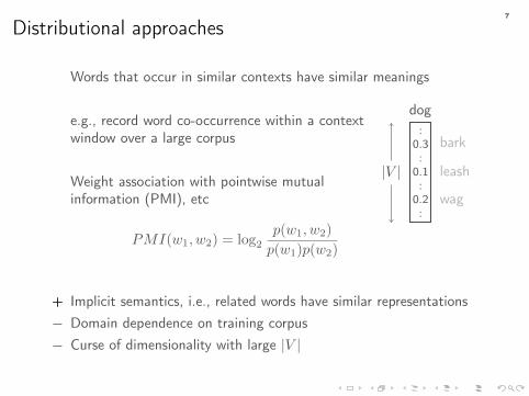
Distributional approaches
Words that occur in similar contexts have similar meanings
e.g., record word co-occurrence within a contextwindow over a large corpus
Weight association with pointwise mutualinformation (PMI), etc
PMI(w1, w2) = log2
p(w1, w2)
p(w1)p(w2)
dog:
0.3:
0.1:
0.2:
bark
leash
wag
|V |
+ Implicit semantics, i.e., related words have similar representations− Domain dependence on training corpus− Curse of dimensionality with large |V |

8
Latent Semantic Analysis Deerwester et al. (1990)Indexing by Latent Semantic Analysis
Construct term-document matrix
M =
|D|
|V |
w(1)1 w
(2)1 · · ·
w(1)2
. . .
...
Singular value decomposition
M ≈ u1 u2 u3 ..
λ1
λ2
λ3
. . .
v1v2v3
:
k
k
Select top k singular vectors for k-dim embeddings of words/docs

9
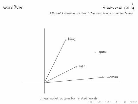
word2vec Mikolov et al. (2013)Efficient Estimation of Word Representations in Vector Space

9
word2vec Mikolov et al. (2013)Efficient Estimation of Word Representations in Vector Space
t-SNE projection of word embeddings from 58k Winemaker’s Noteshttp://methodmatters.blogspot.com/2017/11/using-word2vec-to-analyze-word.html

9
word2vec Mikolov et al. (2013)Efficient Estimation of Word Representations in Vector Space
t-SNE projection of name embeddings from all 7 Harry Potter bookshttps://github.com/nchah/word2vec4everything

9
word2vec Mikolov et al. (2013)Efficient Estimation of Word Representations in Vector Space
king
queen
man
womanuncle
aunt
sir
madam
Linear substructure for related words
9
word2vec Mikolov et al. (2013)Efficient Estimation of Word Representations in Vector Space
king
queen
man
woman
Linear substructure for related words

9
word2vec Mikolov et al. (2013)Efficient Estimation of Word Representations in Vector Space
king
queen
man
woman
king − man
Linear substructure for related words

9
word2vec Mikolov et al. (2013)Efficient Estimation of Word Representations in Vector Space
king
queen
man
woman
king − manking − man + woman
Linear substructure for related words

9
word2vec Mikolov et al. (2013)Efficient Estimation of Word Representations in Vector Space
Analogical reasoning

10
word2vec Mikolov et al. (2013)Distributed Representations of Words and Phrases and their Compositionality
Visualizing lexical relationships

11
word2vec Mikolov et al. (2013)Continuous Bag-of-Words (CBOW)
- Predict target wt given context wt−c, . . . , wt−1, wt+1, . . . , wt+c
wt
`(W,U) = − log p(wt|wt−c · · ·wt+c)
· · · · · ·wt−c wt−1 wt+1 wt+c
W W W W
U
ht =1
2c
c∑i=−ci 6=0
W>wt+i
p(wj |wt−c · · ·wt+c) =eUjht∑k e
Ukht
Input
Projection(averaged)
Softmax
Loss
Label

12
word2vec Mikolov et al. (2013)Skip-gram
- Predict context wt−c, . . . , wt−1, wt+1, . . . , wt+c given target wt
wt−c wt−1 wt+1 wt+c· · · · · ·
`(W,U) = −c∑
i=−ci 6=0
log p(wt+i|wt)
· · · · · ·
wt
W
U U U U
ht = W>wt
p(wj |wt) =eUjht∑k e
Ukht
Input
Projection
Softmax
Loss
Label

13
word2vec Mikolov et al. (2013)
Cost of computing ∇p(wj | · · · ) is proportional to V !
Alternative 1: Hierarchical softmax- Predict path in binary tree representation of output layer- Reduces to log2(V ) binary decisions
p(wt = “dog”| · · · ) = (1− σ(U0ht))× σ(U1ht)× σ(U4ht)
0
1 2
3 4 5 6
cow duck cat dog she he and the
14
word2vec Mikolov et al. (2013)
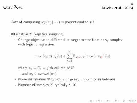
Cost of computing ∇p(wj | · · · ) is proportional to V !
Alternative 2: Negative sampling- Change objective to differentiate target vector from noisy sampleswith logistic regression
max log σ(u>j ht) +
K∑k=1
Ewm∼Ψ log σ(−um>ht)
where uj = Uj = j’th column of Uand wj ∈ context(wt)
- Noise distribution Ψ typically unigram, uniform or in between- Number of samples K typically 5–20

15
word2vec Levy & Goldberg (2014)Neural Word Embedding as Implicit Matrix Factorization
Skip-gram with negative sampling increases u>j ht for realword-context pairs 〈wt, wj〉 and decreases it for noise pairs
Given:· a matrix of d-dim word vectors W (|Vw| × d)· a matrix of d-dim context vectors U (|Vu| × d)
Skip-gram is implicitly factorizing the matrix M = WU>
What is M?- Word-context matrix where each cell (i, j) contains PMI(wi, wj)- If number of negative samples K > 1, this is shifted by a constant− logK
- (Assuming large enough d and iterations)

16
GloVe Pennington et al. (2014)Global Vectors for Word Representation
Similar words have similar ratios of co-occurrence probabilities for contextwords
f((ui − uj)>uk
)=p(wk|wi)
p(wk|wj)
⇒ u>i uk + bi + bk = logcount(wi, wk)
count(wi)
+ Explicitly encodes linear substructure between similar words+ Scales to huge corpora
Pre-trained embeddings at https://nlp.stanford.edu/projects/glove/· Common Crawl: 840B tokens, |V | = 2.2M, d = 300
· Twitter: 27B tokens, |V | = 1.2M, d = 25− 200

16
GloVe Pennington et al. (2014)Global Vectors for Word Representation
Linear substructure (male vs female)

16
GloVe Pennington et al. (2014)Global Vectors for Word Representation
Linear substructure (city vs zip code)

16
GloVe Pennington et al. (2014)Global Vectors for Word Representation
Linear substructure (company vs CEO)

16
GloVe Pennington et al. (2014)Global Vectors for Word Representation
Linear substructure (comparative vs superlative adjectives)

17
word2vec with phrases Mikolov et al. (2013)Distributed Representations of Words and Phrases and their Compositionality
Phrase analogies
Additive compositionality

18
Bilingual word embeddings
Aligned embeddings for English and German (Luong et al., 2015)

19
Resources for word embeddings
Original code and pre-trained embeddings:https://code.google.com/archive/p/word2vec/
Python library for word and document embeddings:https://radimrehurek.com/gensim/models/word2vec.html
Tensorflow tutorial and implementation:https://www.tensorflow.org/tutorials/representation/word2vec
FastText library and pre-trained embeddings for 157 languages:https://github.com/facebookresearch/fastText

20
Beyond words
Can we add word vectors to make sentence/paragraph/doc vectors?doc A = a1 + a2 + a3
doc B = b1 + b2 + b3
cos(A,B) =A ·B
||A|| · ||B||
=1
||A|| · ||B||(a1 · b1 + a1 · b2 + a1 · b3+a2 · b1 + a2 · b2 + a2 · b3+
a3 · b1 + a3 · b2 + a3 · b3)
= weighted all-pairs similarity over A and B

21
Paragraph vector (a.k.a doc2vec) Le & Mikolov (2014)Distributed Representations of Sentences and DocumentsDistributed memory
- Predict target wt given context wt−c, . . . , wt−1, wt+1, . . . , wt+c anddoc label dk
- At test time, hold U , W fixed and back-prop into expanded D
wt
`(W,U,D) = − log p(wt|wt−c · · ·wt+c, dk)
· · · · · ·dk wt−c wt−1 wt+1 wt+c
D W W W W
U
Input
Projection(concatenated)
Softmax
Loss
Label

22
Paragraph vector (a.k.a doc2vec) Le & Mikolov (2014)Distributed Representations of Sentences and Documents
Distributed Bag-of-Words (DBOW)- Predict target n-grams wt, . . . , wt+c given doc label dk- At test time, hold U fixed and back-prop into expanded D
wt wt+c· · ·
`(U,D) = −c∑
i=0
log p(wt+i|dk)
· · ·
dk
D
U U
Input
Projection
Softmax
Loss
Label

23
Semantics are elusive
Visitors saw her duck with binoculars .
Did she duck or does she have a duck?
Who has the binoculars?
How many pairs of binoculars are there?

23
Semantics are elusive
Visitors saw her duck with binoculars .
Did she duck or does she have a duck?
Who has the binoculars?
How many pairs of binoculars are there?

23
Semantics are elusive
Visitors saw her duck with binoculars .NNS VBD PRP$ NN IN NNS .
Did she duck or does she have a duck?
Who has the binoculars?
How many pairs of binoculars are there?

23
Semantics are elusive
Visitors saw her duck with binoculars .NNS VBD PRP VB IN NNS .
Did she duck or does she have a duck?
Who has the binoculars?
How many pairs of binoculars are there?

23
Semantics are elusive
Visitors saw her duck with binoculars .NNS VBD PRP VB IN NNS .
Did she duck or does she have a duck?
Who has the binoculars?
How many pairs of binoculars are there?

23
Semantics are elusive
Visitors saw her duck with binoculars .NNS VBD PRP VB IN NNS .
ccomp
Did she duck or does she have a duck?
Who has the binoculars?
How many pairs of binoculars are there?

23
Semantics are elusive
Visitors saw her duck with binoculars .NNS VBD PRP VB IN NNS .
ccomp
Did she duck or does she have a duck?
Who has the binoculars?
How many pairs of binoculars are there?

23
Semantics are elusive
Visitors saw her duck with binoculars .NNS VBD PRP$ NN IN NNS .
dobj
Did she duck or does she have a duck?
Who has the binoculars?
How many pairs of binoculars are there?

23
Semantics are elusive
Visitors saw her duck with binoculars .NNS VBD PRP$ NN IN NNS .
dobj
Did she duck or does she have a duck?
Who has the binoculars?
How many pairs of binoculars are there?

23
Semantics are elusive
Visitors saw her duck with binoculars .NNS VBD PRP$ NN IN NNS .
dobj
Did she duck or does she have a duck?
Who has the binoculars?
How many pairs of binoculars are there?

24
Recurrent connections
Output vector
Hidden state
Input vector
ht
xt
yt

24
Recurrent connections
Output vector
Hidden state
Input vector
ht
xt
yt
Wxh
Whh
ht = φh(Wxh xt +Whh ht−1)

24
Recurrent connections
Output vector
Hidden state
Input vector
ht
xt
yt
Wxh
Why
Whh
yt = φy(Why ht)
ht = φh(Wxh xt +Whh ht−1)

25
Recurrent connections: Unfolding
x1 x2 x3 x4 · · ·

25
Recurrent connections: Unfolding
x1 x2 x3 x4 · · ·
h1
Wxh

25
Recurrent connections: Unfolding
x1 x2 x3 x4 · · ·
h1
Wxh
y1
Why

25
Recurrent connections: Unfolding
x1 x2 x3 x4 · · ·
h1
Wxh
y1
Why
h2
Wxh
Whh

25
Recurrent connections: Unfolding
x1 x2 x3 x4 · · ·
h1
Wxh
y1
Why
h2
Wxh
Whh
y2
Why

25
Recurrent connections: Unfolding
x1 x2 x3 x4 · · ·
h1
Wxh
y1
Why
h2
Wxh
Whh
y2
Why
h3
Wxh
Whh

25
Recurrent connections: Unfolding
x1 x2 x3 x4 · · ·
h1
Wxh
y1
Why
h2
Wxh
Whh
y2
Why
h3
Wxh
Whh
y3
Why

25
Recurrent connections: Unfolding
x1 x2 x3 x4 · · ·
h1
Wxh
y1
Why
h2
Wxh
Whh
y2
Why
h3
Wxh
Whh
y3
Why
h4
Wxh
Whh

25
Recurrent connections: Unfolding
x1 x2 x3 x4 · · ·
h1
Wxh
y1
Why
h2
Wxh
Whh
y2
Why
h3
Wxh
Whh
y3
Why
h4
Wxh
Whh
y4
Why

25
Recurrent connections: Backprop through time
x1 x2 x3 x4 · · ·
h1
Wxh
y1
Why
h2
Wxh
Whh
y2
Why
h3
Wxh
Whh
y3
Why
h4
Wxh
Whh
y4
Why ∂L∂Why
∂L∂Wxh
∂L∂Whh

25
Recurrent connections: Backprop through time
x1 x2 x3 x4 · · ·
h1
Wxh
y1
Why
h2
Wxh
Whh
y2
Why
h3
Wxh
Whh
y3
Why
h4
Wxh
Whh
y4
Why ∂L∂Why
∂L∂Wxh
∂L∂Whh
∂L∂Wxh
∂L∂Whh
∂L∂Wxh
∂L∂Whh
∂L∂Wxh
25
Recurrent connections: Backprop through time
x1 x2 x3 x4 · · ·
h1
Wxh
y1
Why
h2
Wxh
Whh
y2
Why
h3
Wxh
Whh
y3
Why
h4
Wxh
Whh
y4
Why
∂L∂Whh
∂L∂Whh
∂L∂Whh
∂L∂Wxh
∂L∂Wxh
∂L∂Wxh
∂L∂Wxh
∂L∂Why
∂L∂Why
= ∂L∂y4
∂y4
∂Why

25
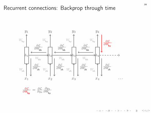
Recurrent connections: Backprop through time
x1 x2 x3 x4 · · ·
h1
Wxh
y1
Why
h2
Wxh
Whh
y2
Why
h3
Wxh
Whh
y3
Why
h4
Wxh
Whh
y4
Why ∂L∂Why∂L
∂Whh
∂L∂Whh
∂L∂Wxh
∂L∂Wxh
∂L∂Wxh
∂L∂Wxh
∂L∂Whh
∂L∂Whh
= ∂L∂y4
∂y4
∂h4
∂h4
∂Whh

25
Recurrent connections: Backprop through time
x1 x2 x3 x4 · · ·
h1
Wxh
y1
Why
h2
Wxh
Whh
y2
Why
h3
Wxh
Whh
y3
Why
h4
Wxh
Whh
y4
Why ∂L∂Why∂L
∂Whh
∂L∂Wxh
∂L∂Wxh
∂L∂Wxh
∂L∂Wxh
∂L∂Whh
∂L∂Whh
∂L∂Whh
= ∂L∂y4
∂y4
∂h4
∂h4
∂Whh+ ∂L
∂y4
∂y4
∂h4
∂h4
∂h3
∂h3
∂Whh

25
Recurrent connections: Backprop through time
x1 x2 x3 x4 · · ·
h1
Wxh
y1
Why
h2
Wxh
Whh
y2
Why
h3
Wxh
Whh
y3
Why
h4
Wxh
Whh
y4
Why ∂L∂Why
∂L∂Wxh
∂L∂Wxh
∂L∂Wxh
∂L∂Wxh
∂L∂Whh
∂L∂Whh
∂L∂Whh
∂L∂Whh
= ∂L∂y4
∂y4
∂h4
∂h4
∂Whh+ ∂L
∂y4
∂y4
∂h4
∂h4
∂h3
∂h3
∂Whh+ ∂L
∂y4
∂y4
∂h4
∂h4
∂h3
∂h3
∂h2
∂h2
∂Whh

25
Recurrent connections: Backprop through time
x1 x2 x3 x4 · · ·
h1
Wxh
y1
Why
h2
Wxh
Whh
y2
Why
h3
Wxh
Whh
y3
Why
h4
Wxh
Whh
y4
Why ∂L∂Why∂L
∂Whh
∂L∂Whh
∂L∂Whh
∂L∂Wxh
∂L∂Wxh
∂L∂Wxh
∂L∂Wxh
∂L∂Wxh
= ∂L∂y4
∂y4
∂h4
∂h4
∂Wxh+ ∂L
∂y4
∂y4
∂h4
∂h4
∂h3
∂h3
∂Wxh+ ∂L
∂y4
∂y4
∂h4
∂h4
∂h3
∂h3
∂h2
∂h2
∂Wxh+
∂L∂y4
∂y4
∂h4
∂h4
∂h3
∂h3
∂h2
∂h2
∂h1
∂h1
∂Wxh
26
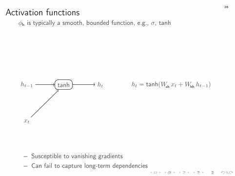
Activation functionsφh is typically a smooth, bounded function, e.g., σ, tanh
ht−1 httanh
xt
ht = tanh(Wxh xt +Whh ht−1)
− Susceptible to vanishing gradients− Can fail to capture long-term dependencies

27
Long short-term memory (LSTM) Gers et al (1999)Learning to Forget: Continual Prediction with LSTM
ct−1
ct
xt
ht−1 tanh +
ct = tanh(Wxh xt +Whh ht−1)
ct = ct−1 + ct

27
Long short-term memory (LSTM) Gers et al (1999)Learning to Forget: Continual Prediction with LSTM
ct−1
ct
xt
ht−1 tanh +
forget×σ
ft = σ(Wfx xt +Wfh ht−1)
ct = tanh(Wxh xt +Whh ht−1)
ct = ft � ct−1 + ct

27
Long short-term memory (LSTM) Gers et al (1999)Learning to Forget: Continual Prediction with LSTM
ct−1
ct
xt
ht−1 tanh +
forget×σ
input×
σ
ft = σ(Wfx xt +Wfh ht−1)
it = σ(Wix xt +Wih ht−1)
ct = tanh(Wxh xt +Whh ht−1)
ct = ft � ct−1 + it � ct
27
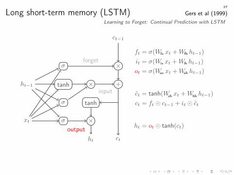
Long short-term memory (LSTM) Gers et al (1999)Learning to Forget: Continual Prediction with LSTM
ct−1
ct
xt
ht−1 tanh +
forget×σ
input×
σ
output
tanh
×
ht
σ
ft = σ(Wfx xt +Wfh ht−1)
it = σ(Wix xt +Wih ht−1)
ot = σ(Wox xt +Woh ht−1)
ct = tanh(Wxh xt +Whh ht−1)
ct = ft � ct−1 + it � ct
ht = ot � tanh(ct)

28
Gated Recurrent Unit (GRU) Cho et al. (2014)Learning Phrase Representations using RNN Encoder-Decoder for Statistical Machine Translation
xt
ht−1
ht
tanh
ht = tanh(Wxh xt +Whh ht−1)
ht = ht

28
Gated Recurrent Unit (GRU) Cho et al. (2014)Learning Phrase Representations using RNN Encoder-Decoder for Statistical Machine Translation
xt
ht−1
ht
tanh
reset
×
σ
rt = σ(Wrx xt +Wrh ht−1)
ht = tanh(Wxh xt +Whh (rt � ht−1))
ht = ht

28
Gated Recurrent Unit (GRU) Cho et al. (2014)Learning Phrase Representations using RNN Encoder-Decoder for Statistical Machine Translation
xt
ht−1
ht
tanh
reset
×
σ
update
×
σ
rt = σ(Wrx xt +Wrh ht−1)
zt = σ(Wzx xt +Wzh ht−1)
ht = tanh(Wxh xt +Whh (rt � ht−1))
ht = zt � ht

28
Gated Recurrent Unit (GRU) Cho et al. (2014)Learning Phrase Representations using RNN Encoder-Decoder for Statistical Machine Translation
xt
ht−1
ht
tanh
reset
×
σ
update
×
σ
1−
×
+
σ
rt = σ(Wrx xt +Wrh ht−1)
zt = σ(Wzx xt +Wzh ht−1)
ht = tanh(Wxh xt +Whh (rt � ht−1))
ht = (1− zt)� ht−1 + zt � ht

29
NLP scenarios: Classification
Given variable-length text w1 · · ·wn (sentence, document, etc), findlabel y
Normal discriminative approach:· Extract features over the input text· Train a linear classifier
Examples:· Topic classification· Sentiment analysis· Entailment recognition
...

30
Classification with RNNs
x1 x2 x3 xn
Wxh Wxh Wxh Wxh
Whh Whh
yWhy
(each xi is a sparse or dense representation of input word wi)

30
Classification with deep RNNs
x1 x2 x3 xn
Wxh Wxh Wxh Wxh
Whh Whh
yW ′
hh W ′hh
Why
+ Can learn more abstract representations− Slow computation because of recurrent dependencies
30
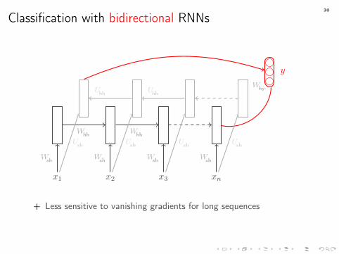
Classification with bidirectional RNNs
x1 x2 x3 xn
Wxh Wxh Wxh Wxh
Whh Whh
y
Why
Uxh Uxh Uxh Uxh
Uhh Uhh
+ Less sensitive to vanishing gradients for long sequences

31
Classification with CNNs Kim (2014)Convolutional Neural Networks for Sentence Classification
· Max-over-time pooling· Two input embedding “channels” — one updated during training

32
Classification with Tree-RNNs Tai et al (2015)Improved Semantic Representations From Tree-Structured Long Short-Term Memory Networks
x1 x2
x3x4 x5
y
WxhWxh
Wxh
Wxh Wxh
Wxh
Why
Computation graph follows dependency or constituency parse(i) Child-sum:
· Good for arbitrary fan-out or unordered children· Suited to dependency trees (input xi is head word)
(ii) N -ary

32
Classification with Tree-RNNs Tai et al (2015)Improved Semantic Representations From Tree-Structured Long Short-Term Memory Networks
x1 x2 x3
y
Wxh Wxh Wxh
W lhh W r
hh
W lhh W r
hh
Why
Computation graph follows dependency or constituency parse(i) Child-sum(ii) N -ary:
· Fixed number of children, each parameterized separately· Suited to binarized constituency parses (leaves take word inputs xi)
33
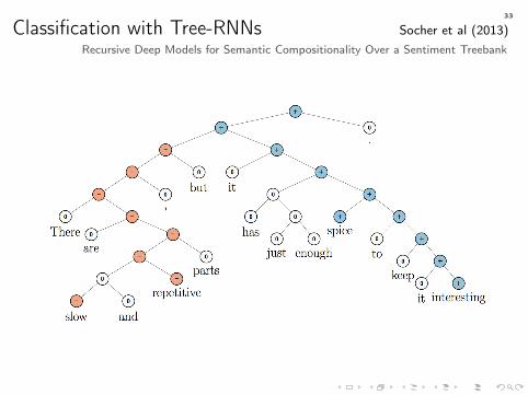
Classification with Tree-RNNs Socher et al (2013)Recursive Deep Models for Semantic Compositionality Over a Sentiment Treebank

34
NLP scenarios: Tagging
Given variable-length text w1 · · ·wn, label spans z1, . . . , zm
Normal discriminative approach:· Distribute labels over input to produce per-word labels y1, . . . , yn
◦ BIO encoding: Beginning-z, Inside-z, Outside◦ BILOU encoding: Beginning-z, Inside-z, Last-z, Outside, Unit-z
· Extract features over input words· Train a linear-chain conditional random field
Examples:· Part-of-speech tagging· Chunking· Named entity recognition· Semantic role labeling
...

35
Tagging with RNNs
x1 x2 x3 x4
Wxh Wxh Wxh Wxh
Whh Whh Whh
y1 y2 y3 y4
Why Why Why Why
+ Effective with BIO/BILOU label encodings

35
Tagging with bidirectional RNNs
x1 x2 x3 x4
Wxh Wxh Wxh Wxh
Whh Whh Whh
y1 y2 y3 y4
Why Why Why Why
Uxh Uxh Uxh Uxh
Uhh Uhh Uhh
+ Effective with BIO/BILOU label encodings+ Less sensitive to vanishing gradients for long sequences

36
NLP scenarios: Generation
Probabilistic language modeling- Distribution over sequences of words p(w1, . . . , wT ) in a language- Typically made tractable via conditional independence assumptions
p(w1, . . . , wn) =
T∏t=1
p(wt|wt−1, . . . wt−n)
- n-gram counts estimated from large corpora- Distributions smoothed to tolerate data sparsity, e.g., Laplace(add-one) smoothing, Kneser-Ney smoothing
- Evaluate on perplexity over held-out data
21N
∑Ni=1 log2 p
(w
(i)1 ...w
(i)Ti
)

37
NLP scenarios: Generation Bengio et al (2003)A Neural Probabilistic Language Model
Discriminative language modeling- Estimate n-gram probabilities with a discriminative model
p(wt|wt−1, . . . w1) ≈ f(w1, . . . , wt)
e.g., model p(wt|wt−1, . . . wt−n) with a feed-forward neural net

38
Language modeling with auto-regressive RNNs
Whh Whh Whh
y1 y2 y3 y4
Why Why Why Why
Wxh Wxh Wxh
· Supply one-hot encoding of output yt as input to timestep t+ 1
· Curriculum learning to overcome model initialization and speed upconvergence

39
RNNLM Mikolov et al (2010)Recurrent Neural Network Based Language Model
Model p(wt|wt−1, . . . wt−n) with an RNNOr an ensemble of multiple RNNs, randomly initialized
Results on Penn Treebank corpus
39
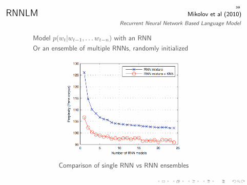
RNNLM Mikolov et al (2010)Recurrent Neural Network Based Language Model
Model p(wt|wt−1, . . . wt−n) with an RNNOr an ensemble of multiple RNNs, randomly initialized
Comparison of single RNN vs RNN ensembles

40
RNNLMs with character CNNs Jozefowicz et al (2015)Exploring the Limits of Language Modeling
Recent models with character-CNN inputs and softmax alternatives

40
RNNLMs with character CNNs Jozefowicz et al (2015)Exploring the Limits of Language Modeling
Nearest neighbors in character-CNN embedding space

41
Transfer learning with NNLMsPre-trained neural language models are useful in classification tasks
Performance gains with ELMo representations added to various models
Deep Contextualized Word Representations (Peters et al., 2018)
Universal Language Model Fine-tuning for Text Classification (Howard and Ruder,2018)
Improving Language Understanding by Generative Pre-Training (Radford et al., 2018)

42
NLP scenarios: Text-to-text
Given variable-length text x1 · · ·xn (sentence, document, etc),produce output text y1, · · · , ym under some transformation
Traditional approaches:· Pipelined models· Constrained optimization
...
Examples:· Machine translation· Document summarization· Sentence simplification· Paraphrase generation
...

43
Decoding with RNNs
Whh Whh
y1 y2 y3
Why Why Why
c
Input context c
Output words y1, . . . , ym

43
Decoding with RNNs
Whh Whh
y1 y2 y3
Why Why Why
c
Wxh Wxh Wxh
Input context c
Output words y1, . . . , ym

43
Encoding with RNNs
x1 x2 xn
Uxh Uxh Uxh
Uhh
Input words x1, . . . , xn
Output representation hn

43
Sequence-to-sequence learning Sutskever, Vinyals & Le (2014)Sequence to Sequence Learning with Neural Networks
Whh Whh
y1 y2 y3
Why Why Why
c
Wxh Wxh Wxh
x1 x2 xn
Uxh Uxh Uxh
Uhh
Input words x1, . . . , xn
Output words y1, . . . , ym

44
Sequence-to-sequence learning Sutskever, Vinyals & Le (2014)Sequence to Sequence Learning with Neural Networks
Produces a fixed length representation of input- “sentence embedding” or “thought vector”

44
Sequence-to-sequence learning Sutskever, Vinyals & Le (2014)Sequence to Sequence Learning with Neural Networks
Produces a fixed length representation of input- “sentence embedding” or “thought vector”

45
Overview: processing text with RNNs
Inputs· One-hot vectors for words/characters/previous output· Embeddings for words/sentences/context
· CNN over characters/words/sentences...
Recurrent layers· Forward, backward, bidirectional, deep· Activations: σ, tanh, gated (LSTM, GRU), ReLU initialized with identity
...
Outputs· Softmax over words/characters/labels
· Absent (i.e., pure encoders)...