karthaus sept. 2007 – slide number 1 numerical modelling of ice sheets and ice shelves tony payne...
TRANSCRIPT
Karthaus Sept. 2007 – Slide Number 1
Numerical modelling of ice sheets and ice shelves
Tony PayneCentre for Polar Observation and Modelling
University of Bristol, U.K.

Karthaus Sept. 2007 – Slide Number 2
Reasons for numerical modelling
o Underlying equations cannot be solved analytically.
o Several different equations that are coupled.
o Irregular geometries when modelling real ice masses.

Karthaus Sept. 2007 – Slide Number 3
Process of numerical modelling
o Continuum mechanics description of problem
o Scaling the equations
o Discretization (quantities no longer in continuous form but represented at finite locations)
o Model coding
o Validation of the model
o Use of the model

Karthaus Sept. 2007 – Slide Number 4
Validating of numerical modelling
o Results from the numerical model are only useful if they can be shown to be independent of the discretization process
o Need to show that results do not vary with time step and grid sizes
– Repeat experiments using a range of grid and time steps
o Numerical models should be tested against any analytical solutions available
o EISMINT benchmarks also very useful in model development

Karthaus Sept. 2007 – Slide Number 5
Types of numerical modelling
o Finite element
– Great freedom in dealing with irregular geometries
– Fairly complicated to develop although software now available to do many of standard tasks
– Computationally demanding
o Finite difference (finite volume)
– Simple to use and develop
– Problems in coping with highly irregular domains

Karthaus Sept. 2007 – Slide Number 6
Basis of finite differences
o Taylor series give a relation between continuous and finite representations
o The series is truncated after a certain number of terms
o The terms omitted give rise to the truncation error of the approximation
o When equations implemented also incur rounding error (due to finite representation of number in memory: use dp)
2 32 3
2 3( ) ( ) ...
2! 3!
t tdH d H d HH t t H t t
dt dt dt

Karthaus Sept. 2007 – Slide Number 7
Taylor series
2 32 3
2 3( ) ( ) ...
2! 3!
t tdH d H d HH t t H t t
dt dt dt
t t+∆t
( )dH
H t tdt
H(t)
H(t +∆t)
22
2( )
2!
tdH d HH t t
dt dt

Karthaus Sept. 2007 – Slide Number 8
Basis of finite differences
2 32 3
2 3
22 3
2 3
2 32 3
2 3
( ) ( ) ...2! 3!
( ) ( )...
2! 3!
( ) ( )( )
( ) ( ) ...2! 3!
( ) ( )( )
t tdH d H d HH t t H t t
dt dt dt
tdH H t t H t d H t d H
dt t dt dt
dH H t t H tO t
dt t
t tdH d H d HH t t H t t
dt dt dt
dH H t H t tO t
dt t
The order of the approximation is the order of the first omitted term

Karthaus Sept. 2007 – Slide Number 9
Basis of finite differences
o In general second-order approximations are sufficient
o In certain circumstances more accurate higher orders may be needed, e.g. near abrupt transitions
2 32 3
2 3
2 32 3
2 3
22
2
2
( ) ( ) ...2! 3!
( ) ( ) ...2! 3!
( ) 2 ( ) ( )( )
3 ( ) 4 ( ) ( 2 )( )
23 ( ) 4 ( ) ( 2 )
2
t tdH d H d HH t t H t t
dt dt dt
t tdH d H d HH t t H t t
dt dt dt
d H H t t H t H t tO t
dt tdH H t H t t H t t
O tdt t
dH H t H t t H t t
dt t
2( )O t

Karthaus Sept. 2007 – Slide Number 10
Stability of finite differences
o Linear instability: Courant-Friedlichs-Lewy constraint on grid size for explicit techniques
o Non-linear instability arises when we try to solve non-linear problems using linear techniques
o In general it manifests itself as high-frequency peaks which grow rapidly
0 1t
cx

Karthaus Sept. 2007 – Slide Number 11
Potted history of numerical modelling
o 1970’s Modelling of glaciers and ice sheets
– 1- and 2-d. models
– zero-order shallow ice approximation
– Mahaffy, Budd, Oerlmans, Pollard, …
– Key techniques: solving non-linear parabolic eqns. in 1 and 2d.

Karthaus Sept. 2007 – Slide Number 12
Potted history of numerical modelling
o 1980’s Ice temperature evolution
– 3d. models
– still zero-order flow models
– Jensen, Huybrechts, Ritz, Greve …
– Key techniques: stretched vertical coordinate

Karthaus Sept. 2007 – Slide Number 13
Potted history of numerical modelling
o 1980’s Modelling of ice shelves and streams
– 2-d. models
– first-order shallow ice approximation but vertically integrated
– MacAyeal, Determann, Thomas …
– Key techniques: solving coupled non-linear elliptic eqns. in 2d.

Karthaus Sept. 2007 – Slide Number 14
Potted history of numerical modelling
o 1990’s Coupled system evolution
– 2d. Ice shelf models
– 3d. Ice sheet, temperature models
– Marshall, Huybrechts, Hulbe …
– Key techniques: internal boundaries

Karthaus Sept. 2007 – Slide Number 15
Potted history of numerical modelling
o 2000’s General ice flow models
– 3-d. models
– first-order shallow ice approximation with no vertically integration
– Pattyn, Blatter, Gudmundsson …
– Key techniques: solving coupled non-linear elliptic eqns. in 3d.
Karthaus Sept. 2007 – Slide Number 16
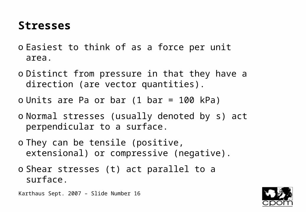
Stresses
o Easiest to think of as a force per unit area.
o Distinct from pressure in that they have a direction (are vector quantities).
o Units are Pa or bar (1 bar = 100 kPa)
o Normal stresses (usually denoted by s) act perpendicular to a surface.
o They can be tensile (positive, extensional) or compressive (negative).
o Shear stresses (t) act parallel to a surface.

Karthaus Sept. 2007 – Slide Number 17
Stress tensor
o Imagine a cube.
o There are three normal stresses corresponding to the three axes
o There are six possible shear stresses
, ,
, ,
, ,
x y z
xy xz yz
yx zx zy

Karthaus Sept. 2007 – Slide Number 18
Stress tensor
o Subscripts denote direction for normal stresses
o Direction perpendicular to surface and then direction acting for shears
o However, reduces to three shears if assume body in equilibrium and can not rotate
yx
xy xy
yx
y
x
yx xy

Karthaus Sept. 2007 – Slide Number 19
Stress equilibrium or force balance
o In glaciology we can neglect acceleration so that Newton’s second law reduces to a force balance
o If there were a force imbalance, acceleration would operate ‘instantaneously’ to restore equilibrium
o Balance is between internal stresses and body forces such as gravity

Karthaus Sept. 2007 – Slide Number 20
Equations of stress equilibrium
Assume static balance of forces by ignoring acceleration
0
0
xyx xz
y xy yz
zy xzz
x y z
y x z
gz y x
g
z
x
y

Karthaus Sept. 2007 – Slide Number 21
Equations of stress equilibrium
( ) ( ) ( ) ( )x xx x x xx x x x x x x
x x
x x+∆x
x

Karthaus Sept. 2007 – Slide Number 22
Equations of stress equilibrium
0
0
xyx xz
xyx xz
y z x x y z x z yx z y
x z y
xxx
∆x
∆y
∆z

Karthaus Sept. 2007 – Slide Number 23
Equations of stress equilibrium
0
0
xyx xz
xyx xz
y z x x y z x z yx z y
x z y
∆x
∆y
∆z
zx xzz zz z

Karthaus Sept. 2007 – Slide Number 24
Equations of stress equilibrium
0
0
xyx xz
xyx xz
y z x x y z x z yx z y
x z y
∆x∆y
∆z
yx xyy yy y

Karthaus Sept. 2007 – Slide Number 25
Equations of stress equilibrium
Assume static balance of forces by ignoring acceleration
0
0
xyx xz
y xy yz
zy xzz
x y z
y x z
gz y x
g
z
x
y

Karthaus Sept. 2007 – Slide Number 26
Strain rates
o Strain is a measure of the deformation of an object
o Typically ratio of a length before deformation to one after (proportional change) and has no units (i.e. is a ratio)
o A strain rate is simply the rate at which this happens.
o Denoted by epsilon dot (dot shows that it is rate) and has units of yr-1

Karthaus Sept. 2007 – Slide Number 27
Strain rates
o Defined as gradients in velocity
o Strain can be normal (simple extension or contraction)
o Or shear which changes shape
o Six strain rates that are equivalent to six stresses
1
2
x
xy
u
x
u v
y x
dx
v1
u1
v2
u2dy
y
x

Karthaus Sept. 2007 – Slide Number 28
Glen’s flow law
A is related to temperature and impurities
n is a constant equal to 3
is effective stress (measure of overall stress regime)
is effective strain rate
nA 1nij ijA
relates to strain rates to stress deviators
Karthaus Sept. 2007 – Slide Number 29
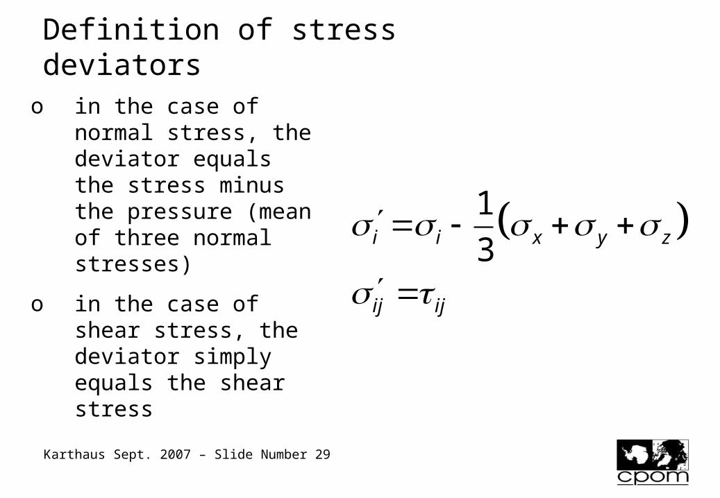
Definition of stress deviators
o in the case of normal stress, the deviator equals the stress minus the pressure (mean of three normal stresses)
o in the case of shear stress, the deviator simply equals the shear stress
1
3i i x y z
ij ij

Karthaus Sept. 2007 – Slide Number 30
Effective stresses
o Measure of total stress environment
o Also for strains
2 2 2 2 2 2 22 2x y z xy xz yz
Karthaus Sept. 2007 – Slide Number 31
Shallow-ice approximation(s)
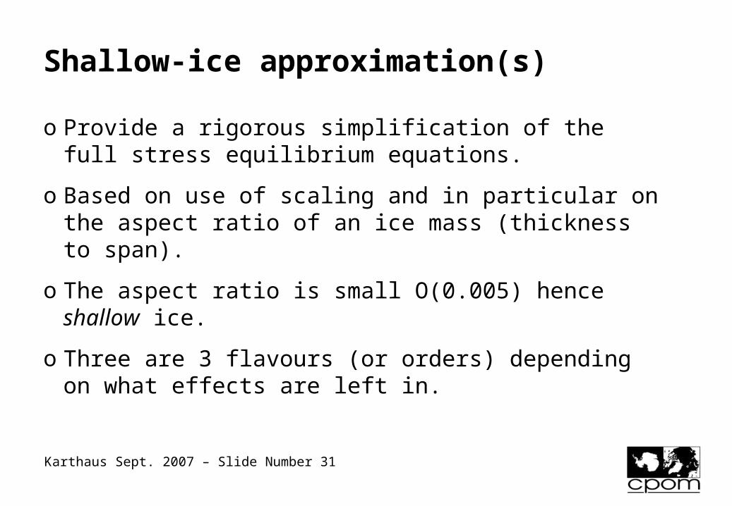
o Provide a rigorous simplification of the full stress equilibrium equations.
o Based on use of scaling and in particular on the aspect ratio of an ice mass (thickness to span).
o The aspect ratio is small O(0.005) hence shallow ice.
o Three are 3 flavours (or orders) depending on what effects are left in.

Karthaus Sept. 2007 – Slide Number 32
Equations of stress equilibrium
Assume static balance of forces by ignoring acceleration
0
0
xyx xz
y xy yz
zy xzz
x y z
y x z
gz y x
g
z
x
y

Karthaus Sept. 2007 – Slide Number 33
Scaling
o Replace variable with a constant scale multiplied by a scaled variable
o allows size of different terms to be compared without further analysis
o Scaled variable should always be O(1)
0
0
original variable
constant scale
scaled variable
H H H
H
H
H

Karthaus Sept. 2007 – Slide Number 34
Scaling
0 0 0
0
0
20
00
z H z x X x y X y
H
X
gHgH
X

Karthaus Sept. 2007 – Slide Number 35
Word on stress deviator scaling
o Some justification for this scale comes from the condition at the ice mass’ upper/lower boundary
o At the upper surface, stress components must balance
00 0
0
20
00
0
0
xz x
xz x
s
xH s
T gHX x
gHT
X

Karthaus Sept. 2007 – Slide Number 36
“Glaciology is a ONE BAR subject” (or 100 kPa in S.I.)

Karthaus Sept. 2007 – Slide Number 37
Vertical equation
Scale equations (note have dropped tildas from scaled variables)
2 20 0 0
2 20 0 0
2 2 1
zy xzz
zy xzz
H H Hg g
H z X y X x
z y x

Karthaus Sept. 2007 – Slide Number 38
Horizontal equations
Scale equations (note have dropped tildas from scaled variables)
2 20 0 0
20 0 0 0
2
2
0
0
0
xyx xz
xyx xz
y xy yz
H H Hg
X x X y H X z
x y z
y x z

Karthaus Sept. 2007 – Slide Number 39
Zero-order approximation
Retain highest order (biggest) terms in each equation
2
2
2 2
0
0
1
xyx xz
y xy yz
zy xzz
x y z
y x z
z y x

Karthaus Sept. 2007 – Slide Number 40
Zero-order approximation
Retain highest order (biggest) terms in each equation
0
0
1
x xz
y yz
z
x z
y z
z

Karthaus Sept. 2007 – Slide Number 41
Zero-order approximation
Easier to move back to unscaled version of equations now
xz x
yz y
z
z x
z y
gz

Karthaus Sept. 2007 – Slide Number 42
Higher-order approximations
Successively include smaller terms
2
2
2 2
0
0
1
xyx xz
y xy yz
zy xzz
x y z
y x z
z y x

Karthaus Sept. 2007 – Slide Number 43
First-order approximation
Successively include smaller terms
2
2
2
0
0
xyx xz
y xy yz
zyz
x y z
y x z
z y
2 xz
x
1

Karthaus Sept. 2007 – Slide Number 44
Second-order approximation
Successively include smaller terms
2
2
2 2
0
0
1
xyx xz
y xy yz
zy xzz
x y z
y x z
z y x

Karthaus Sept. 2007 – Slide Number 45
Quick zero-order derivation
o assume on basis of aspect ratio that
normal stress dominates in vertical
vertical shear dominates horizontal shear
xyx
x y
0xz
y xy
z
y x
0yz
zyz
z
z y
xz
x
g

Karthaus Sept. 2007 – Slide Number 46
Quick zero-order derivation
o Integrate vertical stress balance
o It can be shown that all normal stresses are equal (i.e. that the pressure is hydrostatic)
0
0
( ) ( )
x xz
y yz
z
z x y
x z
y z
z g s z

Karthaus Sept. 2007 – Slide Number 47
Quick zero-order derivation
0
0
xz
yz
g s zx z
g s zy z
o Substitute horizontal normal stresses with vertical normal stress

Karthaus Sept. 2007 – Slide Number 48
Quick zero-order derivation
0
0
( ) ( )
( ) ( )
xz
yz
xz
yz
sg
x z
sg
y z
sz g s z
xs
z g s zy
o Tidy up
o Gravitational driving stress (RHS) balanced entirely by vertical shear (LHS)
o For whole ice column gravitational driving is balanced locally by basal drag alone

Karthaus Sept. 2007 – Slide Number 49
Quick zero-order approximation
Normally used in combination with Glen’s flow law
1
2xz
u w
z x
1
2 22
nxz
x
A
2y 2
z 22 xy 2 2xz yz

Karthaus Sept. 2007 – Slide Number 50
Quick zero-order approximation
Shown that vertical shear stresses are only important ones
1
2 2 2
2
ˆ
ˆ
nxz
xz yz
xz
yz
uA
z
sg s z
xs
g s zy

Karthaus Sept. 2007 – Slide Number 51
Quick zero-order approximation
Integrate from bed to some height within ice to get velocity
12 2 2
1ˆ2 2 2
ˆ2
ˆ ˆ2
n
n
nz
n n
h
u s s sA g s z
z x y x
s s su z g A s z dz
x y x
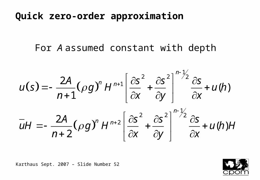
Karthaus Sept. 2007 – Slide Number 52
Quick zero-order approximation
For A assumed constant with depth
12 2 2
1
12 2 2
2
2( )
1
2( )
2
n
n n
n
n n
A s s su s g H u h
n x y x
A s s suH g H u h H
n x y x

Karthaus Sept. 2007 – Slide Number 53
Simple glacier flow model: 1-d. equations
1
22( )
2
nn nA s s
uH g H u h Hn x x

Karthaus Sept. 2007 – Slide Number 54
Simple glacier flow model: 1-d. equations
o Ice thickness (H) evolution
o Zero order model of ice flow (u)
o Mass balance model (b)
o Here simplified by assuming flat bed
112 ( )
2
nnn
H Hub
t x
A g s su H
n x x

Karthaus Sept. 2007 – Slide Number 55
Simple glacier flow model: 1-d. equations
o Mass balance model (b)
o Nonlinear (D) parabolic equation
o Here simplified by assuming flat bed 1
22 ( )
2
nnn
s sb D
t x x
A g sD H
n x

Karthaus Sept. 2007 – Slide Number 56
Glacier model: spatial discretization
o Regular 1-d. grid
o Staggered so that fluxes evaluated halfway between cells
1
1/ 2
1
1/ 2
1/ 21/ 2
2
,
i i
i
i i
i
ii
s ss
x x
D D
Ds
D Hx
GRID i-1 i-½ i i+½ i+1
H,s,b ○ ○ ○
∂s/∂x ● ●
D(1) ○ ● ○ ● ○
D(2) ● ●

Karthaus Sept. 2007 – Slide Number 57
Glacier model: spatial discretization
o Substitute FD fluxes
1 11/ 2 1/ 2
1 1/ 2 1 1/ 2 1/ 2 1/ 22
1
1
i i i ii i i
i i i i i i i i
s s s ssb D b D D
x x x x x
b s D s D s D Dx

Karthaus Sept. 2007 – Slide Number 58
Glacier model: spatial discretization
o Forms a tridiagonal matrix
1.5 2.5 1.5 2.5 2 2
2.5 3.5 2.5 3.5 3 32
3.5 4.5 3.5 4.5 4 4
. . . .
1
. . . .
D D D D s b
D D D D s bx
D D D D s b

Karthaus Sept. 2007 – Slide Number 59
Glacier model: explicit time discretization
o First-order, forward approximation to time derivative
o Disadvantages: first-order error (Taylor’s) and not very stable (CFD limit)
i-1 i-½ i i+½ i+1
time ○ ● ○ ● ○
time + dt ○
1i i
i
s ss
t t

Karthaus Sept. 2007 – Slide Number 60
Glacier model: fully implicit discretization
o First-order, backward approximation to time derivative
o still first-order error
o but now far more stable
o however need to evaluate flows a new time step
i-1 i-½ i i+½ i+1
time ○
time + dt ○ ● ○ ○ ●
1
1
i i
i
s ss
t t

Karthaus Sept. 2007 – Slide Number 61
Glacier model: implicit solution
o Use direct Gaussian solver on tridiagonal (NR)
o No additional computing cost compared to explicit
o Stable as long as diagonally dominant (i.e. always in this case)
1.5 2.5 1.5 2.5 2 2 2
2.5 3.5 2.5 3.5 3 3 3
3.5 4.5 3.5 4.5 4 4 4
1/ 2 1/ 2 2
. . . .
1
1
1
. . . .
i i
E E E E s s b
E E E E s s b
E E E E s s b
tE D
x

Karthaus Sept. 2007 – Slide Number 62
Glacier model: semi-implicit discretization
o Second-order, centred approximation to time derivative (Crank-Nicolson)
o need to evaluate flows at both time steps
i-1 i-½ i i+½ i+1
time ○ ● ○ ○ ●
time + dt ○ ● ○ ○ ●
1
1/ 2
i i
i
H HH
t t

Karthaus Sept. 2007 – Slide Number 63
Glacier model: non-linear instability
o Diffusivity (D) is a highly non-linear function of thickness (power 5) and surface slope (power 2)
o Good type problem for methods later on
o Options:
– Ignore the problem (just use D from previous time step)
– Picard iteration
– Under-relaxation, Hindmarsh schemes
– Newton-Raphson iteration

Karthaus Sept. 2007 – Slide Number 64
Glacier model: Picard iteration
Calculate Dfrom H, s
Solve for new Sgiven D
DONE
Check forconvergence

Karthaus Sept. 2007 – Slide Number 65
Glacier model: relaxation and Hindmarsh
o Non-linear instability manifests itself as high-frequency oscillation as numerical solution over corrects past the ‘true’ solution but never finds it
o Under-relaxation reduces the correction applied in each iteration and makes convergence more likely
o The scheme published by Hindmarsh and Payne (1996) recognises the (chaotic) oscillatory behaviour and aims for the ‘mid-point’
iterationsH

Karthaus Sept. 2007 – Slide Number 66
Glacier model: Newton-Raphson solver
o Recognises the non-linear nature of the problem fully
o Very fast convergence
o More complicated to programme but MAPLE etc makes evaluation of Jacobian easy
1
1 1
FD ( )
( ) ( ) ( )
( )
. . .. .
, ,
. .. . .
k k kk k ki i ii i ik k k
i i i
s sf b D s
t x x
f s ds f s f sf s
ds dsf s
dsf s
f f fs s f
s s s

Karthaus Sept. 2007 – Slide Number 67
Glacier model: final comments
o Can insert expressions for basal slip but these typically make assumption about all gravitational driving balanced locally
o Strictly only appropriate at grid scales 10-20 times ice thickness
o Easily coupled to simple mass balance – climate models (also isostasy)
o Very successful in explaining features of Ice Ages
o VERIFY numerics by comparing the Nye-Vialov steady-state profiles

Karthaus Sept. 2007 – Slide Number 68
Examples
This type of model was very useful in understanding causes of Ice Ages and relation to Milankovitch forcing
snowline

Karthaus Sept. 2007 – Slide Number 69
Examples
Coupled via snowline to simple climate models.
Used to explain disparity between forcing and response

Karthaus Sept. 2007 – Slide Number 70
Examples
Range of experiments showed that 100 kyr cycles could be reproduced if extra physics added to cause ‘fast’ deglaciation
Pollard, 1982

Karthaus Sept. 2007 – Slide Number 71
Simple ice sheet model: 2-d. equations
o 2-d. version of previous non-linear parabolic equation
o Very similar derivation
o 2-d. nature of problem increases complexity of numerics
1
2 2 22
.
2 ( )
2
nn
n
H s sb D s b D D
t x x y y
A g s sD H
n x y

Karthaus Sept. 2007 – Slide Number 72
Simple ice sheet model: spatial discretization
o Number of choices for how quantities calculated on staggered grid
o Problem originally studied in GCM by Arakawa
o C-grid traditionally used by glaciologists although B may have advantages

Karthaus Sept. 2007 – Slide Number 73
Simple ice sheet model: spatial discretization
o Problems with evaluating all derivatives on C-grid
o B-grid more symmetrical
● flux
○ thickness
i-1 i-½ i i+½ i+1
j+1 ○ ○ ○
j+½ ●
j ○ ● ○ ● ○
j-½ ●
j-1 ○ ○ ○
i-1 i-½ i i+½ i+1
j+1 ○ ○ ○
j+½ ● ●
j ○ ○ ○
j-½ ● ●
j-1 ○ ○ ○

Karthaus Sept. 2007 – Slide Number 74
Simple ice sheet model: implicit solution
o No longer have simple tridiagonal matrix
o This means direct (Gaussian) methods of solution will be very, very expensive
o Need to look towards iterative methods …
1 1 1 1
1 1
1 1 1 1
1 1
1 1
1 1
1
1 1
. .. .
. .. .
i j i j
ij ij
i j i j
i j i j
ij ij
i j i j
i j i
ij
i j
H bD
H bD
H bD
H bU D L D U L D U
H bL D U L D U L D U
H bL D U L D U D U
H bL D U
HL D U
HL D
1 1
1
1 1
j
ij
i j
b
b
A.x=b

Karthaus Sept. 2007 – Slide Number 75
Simple ice sheet model: matrix solvers
o The traditional method (i.e., explicit) uses a point iteration
o The convergence of the technique can be improved by over-relaxation (SOR)
o Could use line inversion (alternating direct implicit, ADI)

Karthaus Sept. 2007 – Slide Number 76
Simple ice sheet model: matrix solvers
o Conjugate gradient methods are ideally suited
o Commonly available as library routines that can be easily incorporated
o Numerical recipes or SLAP library (which offers many preconditioners)
o All use sparse matrix storage
o Multigrid techniques now popular in many other fields but untried in glaciology
1( )
2f x
f
A.x b
x.A.x -b.x
A.x b

Karthaus Sept. 2007 – Slide Number 77
Examples
Type of model was work horse of modelling community and has produced many of the simulations on which previous IPCC reports are based (eg Huybrechts and de Wolde 1999)

Karthaus Sept. 2007 – Slide Number 78
Reasons for interest in temperature
o Determines whether water present at the bed
– ice frozen to bed exerts greater traction
– meltwater allows lubrication and reduced traction
– all known ice streams have water at the bed
o Determines the softness of ice
– warm is deforms more rapidly
– very large effect over natural temp. range

Karthaus Sept. 2007 – Slide Number 79
Ice temperature evolution : equations
o Vertical diffusion
o Vertical advection
o Horizontal advection
o Dissipation
o Local rate of change
o Upper boundary condition: air temperature
o Lower boundary condition: geothermal heat flux
2
2
z s a
z h
T k T T T Tw u v
t C z z x y C
T T
T G
z k

Karthaus Sept. 2007 – Slide Number 80
Potential coupling to ice flow?
o Effect of thicker ice?
o Effect of increased driving stresses?
o Effect of faster velocities?
o Effect of warmer temperatures?
2
2
z s a
z h
T k T T T Tw u v
t c z z x y c
T T
T G
z k

Karthaus Sept. 2007 – Slide Number 81
Ice temperature evolution: numerics
o Treat as column model with horizontal terms as corrections
o 1-d. diffusion equation can be solved using previous methods
o Additional techniques needed:
– Boundary conditions
– Advection terms
– Stretched vertical coordinate

Karthaus Sept. 2007 – Slide Number 82
Temperature evolution : upper boundary
o Dirichlet boundary condition
o Simply use air temperature at k = 1
1 1 1
11
2,
t t t tt t k k k k
k k
ta
T T T Tt kT T
z C z z
k n
T T

Karthaus Sept. 2007 – Slide Number 83
Temperature evolution : lower boundary
o von Neumann or flux boundary condition
o Use boundary condition to supply extra equation for n+1
o Substitute this into original approximation at n
1 1 1
1 11 1
1 11 1
112
2,
2
2
2 2
t t t tt t k k k k
k k
t tn n
t tn n
t t t tn n n n
T T T Tt kT T
z C z z
k n
T T G
z kG
T T zk
t k t GT T T T
z C z C

Karthaus Sept. 2007 – Slide Number 84
Ice temperature evolution: advection
o Number of options for first derivatives associated with advection
– Centred, second order
– Non-centred, first order
– Non-centred, second order
o Centred derivative is unconditional unstable (solution splits)
o Non-centred, first order introduces excessive artificial diffusion
1 1
1 1
2 1 1 2
2
,
4 3 3 4,
2 2
i i
i i i i
i i i i i i
T T
xT T T TT
x x xT T T T T T
x x

Karthaus Sept. 2007 – Slide Number 85
Ice temperature evolution: advection
o Non-centred, second order normally produces satisfactory results if used as part of an upwinding scheme
2 1
1 2
4 3
2 2
3 4
2 2
k k i i i
k k i i i
u u T T TTu
x x
u u T T T
x
Karthaus Sept. 2007 – Slide Number 86
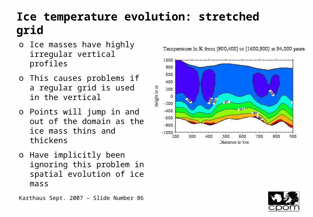
Ice temperature evolution: stretched grid
o Ice masses have highly irregular vertical profiles
o This causes problems if a regular grid is used in the vertical
o Points will jump in and out of the domain as the ice mass thins and thickens
o Have implicitly been ignoring this problem in spatial evolution of ice mass

Karthaus Sept. 2007 – Slide Number 87
Ice temperature evolution: stretched grid
o Grid stretching is a technique that ensures the grid always fits to the local ice thickness
o Also ensures that boundaries always lie on grid points (hence boundary conditions easier to employ)
o However does add the complexity of equations
( )
( ) 0
( ) 1
s zz
Hs
h

Karthaus Sept. 2007 – Slide Number 88
Ice temperature evolution : stretched grid
o Need to add terms to deal with deformed grid
o This is easy for terms in z
2 2
2 2 2
1
1
1
T T
z zs z
z z H H
T T
z H
T T
z H

Karthaus Sept. 2007 – Slide Number 89
Ice temperature evolution: stretched grid
o But trickier for other terms which in t, x, and y
o If this is done with each term then an ‘apparent velocity’ for the grid can be found
*
*
1
z
T T T
x x x
s z
x x H
s H
x H x x
w u vt x y
w wT T
t H

Karthaus Sept. 2007 – Slide Number 90
Ice temperature evolution: stretched grid
o An irregularly spaced grid is often used in the vertical, stretched coordinate
o Points are concentrated near the bed (most deformation)
o This does increase truncation error (non centred)
o Better alternative is to use non-linear coordinate
( )exp 1
exp( ) 1
( ) 0
( ) 1
a s zHa
z s
z h

Karthaus Sept. 2007 – Slide Number 91
Ice temperature evolution: tidying up
o Horizontal velocities still come from zero order shallow ice model
o Vertical velocities found using incompressibility condition
o Numerical integration from bed to surface (Trapezoidal Rule, NR)
o Test of integration accuracy from surface kinematic boundary condition
( ) ( )
( ) ( )
w u v
z x y
h h hw h u h u h M
t x xs s s
w s u s u s bt x x

Karthaus Sept. 2007 – Slide Number 92
Ice temperature evolution: uses
o Work coupling melt rates to simple local water storage model

Karthaus Sept. 2007 – Slide Number 93
Ice temperature evolution: uses
o Interaction between flow, temperature and basal water can lead to interesting results …
Karthaus Sept. 2007 – Slide Number 94
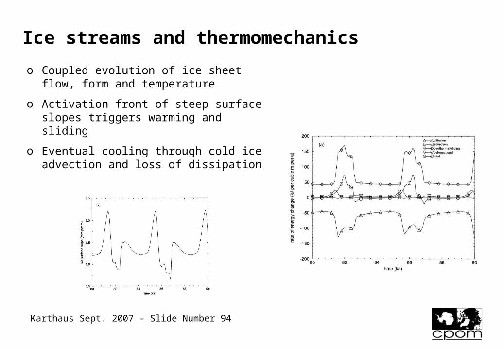
Ice streams and thermomechanics
o Coupled evolution of ice sheet flow, form and temperature
o Activation front of steep surface slopes triggers warming and sliding
o Eventual cooling through cold ice advection and loss of dissipation
Karthaus Sept. 2007 – Slide Number 95
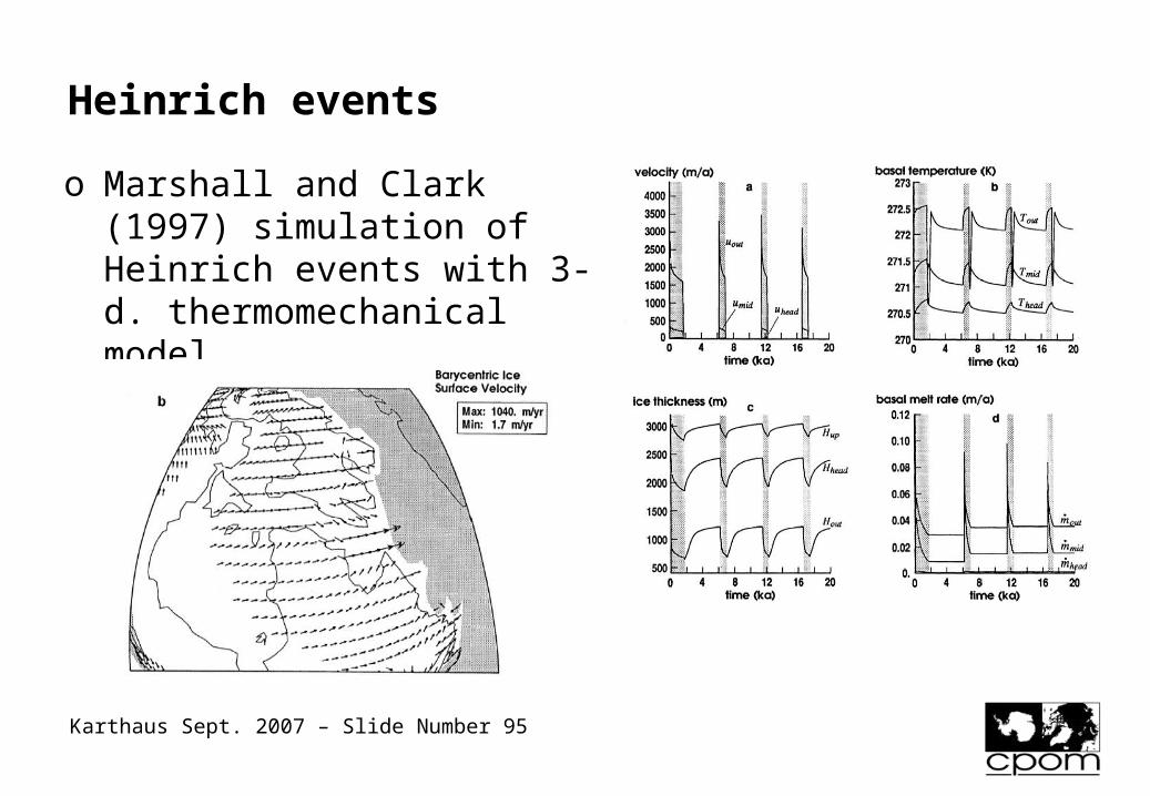
Heinrich events
o Marshall and Clark (1997) simulation of Heinrich events with 3-d. thermomechanical model

Karthaus Sept. 2007 – Slide Number 96
EISMINT thermomechanical results
o Comparison of 10 ice sheet models with thermomechanical coupling (Payne and others 2000)
o Results show sensitivity details of numerics
o Hindmarsh (2004) uses normal modes to show that while feedback exists it is relatively weak (hence numerical problems)

Karthaus Sept. 2007 – Slide Number 97
Ice temperature evolution: uses
o Also for Antarctica …
log10(|U|)

Karthaus Sept. 2007 – Slide Number 98
Ice shelf models: derivation
o Still assume that vertical balance is dominated by normal stress gradient
o Show remainder of derivation for 1-d. confined shelf
0
0
xyx xz
y xy yz
zyz
x y z
y x z
z y
xz
x
g

Karthaus Sept. 2007 – Slide Number 99
Ice shelf models: derivation
o Repeat zero-order proceedure
o Left with additional stress deviator term
0
1
2
2
x xz
z
x x x z
x xz
x zg s z
sg
x z x

Karthaus Sept. 2007 – Slide Number 100
Ice shelf models: derivation
o Integrate through ice thickness
o Apply Leibniz rule
( ) ( )
( ) ( )
2
( , ) ( ( ), ) ( ( ), )
( ) ( )
s s sx xz
h h h
b x b x
a x a x
s sx
x x x
h h
sdz dz g dz
x z x
f b adz f z x dz f b x x f a z x
x x x x
s hdz dz s h
x x x x

Karthaus Sept. 2007 – Slide Number 101
Ice shelf models: derivation
o Subsititute boundary conditions for stresses
( ) ( )
( ) ( )
( ) ( )
xz x
xz x
s sx
x xz x
x
z x
h h
b
b
ss s
xh
h hx
dz dz s hx x

Karthaus Sept. 2007 – Slide Number 102
Ice shelf models: derivation
o Perform remaining integrations
o Terms cancel etc.
2 ( ) ( )
2
s s sxz
x xz xz bx
h h h
x bx
sdz s h dz g dz
x z x
sH gH
x x

Karthaus Sept. 2007 – Slide Number 103
Ice shelf models: derivation
o Two 2-d. vertically integrated equations
o also used to study ice streams with inclusion of a basal drag term
o Linear slip law normally used
o Up to this point the derivation is general
2
2
2
2
xyx y bx
xyy x by
bx
by
sH H gH
x y x
sH H gH
y x y
u
v

Karthaus Sept. 2007 – Slide Number 104
Ice shelf models: derivation
o Normally solved by replacing stress deviators with strain rates
o Inverse form of Glen’s flow law
o Define an effective viscosity (f)
1
1
1
12
12
1 1
2
x n
y n
xy n
u uf
A x xv v
fA y y
u v u vf
A y x y x

Karthaus Sept. 2007 – Slide Number 105
Ice shelf models: derivation
o Problem is that need vertically averaged quantities for stresses and velocities etc.
o No simple relation between these averages if vertical shear is present
o Must assume (e.g., MacAyeal) that no variation in the vertical
o This limits application to true ice shelves or shelfy ice streams
2xu
fx

Karthaus Sept. 2007 – Slide Number 106
Ice shelf models: derivation
o Effective viscosity can also be found in terms of strain rates
11
1/ (1 ) /
(1 ) / 22 221/
1
21
2
1 1
2 4
n
n n n
n n
n
f A
f A
u v u v u vf A
x y x y y x

Karthaus Sept. 2007 – Slide Number 107
Ice shelf models: derivation
o Final equations are coupled non-linear elliptical equations in u and v
o Non-linearity enters via effective viscosity
2 2
2 2
u v u v sf H f H gH
x x y y y x x
v u u v sf H f H gH
y y x x y x y

Karthaus Sept. 2007 – Slide Number 108
Ice shelf models: solution
o Solve for u given v, and vice versa
o Use previous techniques for 2-d. parabolic equations (conjugate gradients)
o Deal with non-linearity using previous techniques also
4
2
4
2
u ufH fH
x x y y
s v vgH fH fH
x x y y x
v vfH fH
y y x x
s u ugH fH fH
y y x x y

Karthaus Sept. 2007 – Slide Number 109
Ice shelf models: boundary conditions
o Kinematic: specify a velocity either from
– observations (if modelling shelf in isolation) or
– zero-order model (if coupling to an ice sheet model)
o Dynamic: specify a stress
– Appropriate to front of ice shelf
– Balance of forces with displaced water
Hh
12
12
xx x xy y
w
yy y xy x
w
n gHn n
n gHn n

Karthaus Sept. 2007 – Slide Number 110
Ice shelf models: boundary conditions
o Dynamic boundary condition messy
o Greatly simplified if implemented so that shelf front aligned along x or y
o Problem when modelling irregular shaped shelves
o Use an artificial shelf with arbitrarily low thickness to extend shelf to domain edge
1, 0
12
0
x y
xw
xy
n n
gH

Karthaus Sept. 2007 – Slide Number 111
Ice shelf models: thickness evolution
o Surface elevation can be found from buoyancy
o Ice thickness evolution can no longer be coupled with velocity calculation
o Must be solved separately
w i
w
s H
H uH uHb
t x y

Karthaus Sept. 2007 – Slide Number 112
Ice shelf models: thickness evolution
o Number of alternatives
– Convert velocities to diffusivities and use old method
– Solve using simple schemes for hyperbolic equations (e.g. staggered leapfrog etc)
– Use more complex transport scheme (e.g. semi-lagrangian methods)
o A satisfactory general solver has yet to be found
1 1
1/ 2 1/ 2
/
2 t tt ti i i i
uD
H xH H
b Dt x x
H uHb
t xt
H H uH uHx

Karthaus Sept. 2007 – Slide Number 113
Ice shelf model: algorithm
Solve for u given f, v
Check forconvergence
Solve for v given f, u (old)
Calculate for f given u, v
Calculate new thickness distribution
Calculate new gravitational driving stress and boundary
conditions

Karthaus Sept. 2007 – Slide Number 114
Davis and others (2005) use ERS alimetry to determine change in surface elevation over last decade
Antarctic mass balance

Karthaus Sept. 2007 – Slide Number 115
Comparison with ERA-40 climate reanalysis for 1980 to 2001 for precipitation
Antarctic mass balance

Karthaus Sept. 2007 – Slide Number 116
Interest in Pine Island Glacier
o PIG has the largest discharge (66 Gt yr-1) of all WAIS ice streams
o with Thwaites Glacier, it drains 40% of the WAIS
o little studied in comparison to Siple Coast ice streams

Karthaus Sept. 2007 – Slide Number 117
Interest in Pine Island Glacier
ogrounding line retreated 8 km between 1992 and 1994
oimplies ice thinning at the grounding line of the order of 3.5 m yr-1
oradar altimetry shows widespread thinning
othinning pattern extends 150 km from grounding line
othinning maps on to template of fast flowing section of ie stream

Karthaus Sept. 2007 – Slide Number 118
Interest in Pine Island Glacier
o thinning unlikely to be related to snowfall variation
o hypothesized causes of thinning:
a) internal flow mechanics of ice stream (surging?)
b) long-term response to climate change (LGM?)
c) recent collapse of ice shelf and/or change in grounding

Karthaus Sept. 2007 – Slide Number 119
Outline of modelo Vertically-integrated
‘MacAyeal’ model includes
– momentum balances in x and y
– assumes vertical shear minimal
– viscous flow law
– dynamic b.c. at shelf front
o Prognostic thickness evolution but based on perturbations to ice flow
2
2
2
2
.
x y xy
y x xy
iref
sH H H u gH
x y y x
sH H H v gH
y x x y
H HUH
t t
• Same domain and grid• Ice surface now two dimensional• Time steps: 0.01 yr for H and 0.1 yr
for u/v (fast wave speeds)

Karthaus Sept. 2007 – Slide Number 120
Used to study Pine Island Glacier
Dynamic b.c.(stress)
Shallow ice model
‘MacAyeal’ stream
‘MacAyeal’ shelf
Kinematic b.c.(velocity)
Thickness evolution
throughout

Karthaus Sept. 2007 – Slide Number 121
Results: surface lowering in m after 0 yr

Karthaus Sept. 2007 – Slide Number 122
Results: surface lowering in m after 2 yr
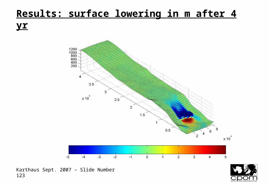
Karthaus Sept. 2007 – Slide Number 123
Results: surface lowering in m after 4 yr

Karthaus Sept. 2007 – Slide Number 124
Results: surface lowering in m after 7 yr

Karthaus Sept. 2007 – Slide Number 125
Results: surface lowering in m after 10 yr
Karthaus Sept. 2007 – Slide Number 126
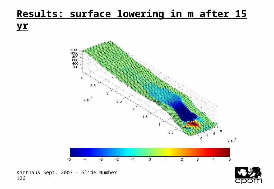
Results: surface lowering in m after 15 yr

Karthaus Sept. 2007 – Slide Number 127
Results: surface lowering in m after 20 yr

Karthaus Sept. 2007 – Slide Number 128
Results: surface lowering in m after 35 yr

Karthaus Sept. 2007 – Slide Number 129
Results: surface lowering in m after 50 yr

Karthaus Sept. 2007 – Slide Number 130
Results: accumulated thinning after 150 yr.
after 50 yr
Total thinning produced
by a range of 2
changes near the
grounding line
Karthaus Sept. 2007 – Slide Number 131
General ice-flow models: derivation
o Both the ice sheet and shelf models are limited in their applicability by the assumptions that are made in their derivation
o Ice sheet models assume local stress balance, and are only strictly applicable at 10-20 time ice thickness
o Ice shelf models assume no vertical shear
o Many problems in glaciology lie between these two extremes, e.g.
– Many (most) ice streams
– Onset areas and shear margins
– Valley glaciers
– Ice divides (coring locations)

Karthaus Sept. 2007 – Slide Number 132
General ice-flow models: derivation
o This motivates development of general models
o Approach is similar to ice shelf model but vertical shear terms are not discarded
o Stretched coordinates are again used
o But second derivatives in x introduce much complexity
(1 ) / 222 21/
2
2
2
2
1 12
2 2
1 1
2 2
ˆ ˆˆ ˆ
ˆ ˆˆ ˆ
xyx xz
n n
n
sg
x y z x
u u u sf f f g
x x y y z z x
u u uf A
x y z
u u uf f f
x x x x x
u uf f
x x x
ˆˆ uf
x

Karthaus Sept. 2007 – Slide Number 134
Dangers of numerical modelling
o Tendency to treat model as a black box or a surrogate for reality.
o Cannot simply use ‘the model says …’ without proving that the model solves the underlying equations satisfactorily and that processes being described are realistic consequences of the equations.