kenward â€“ roger's approach - oregon state university

AN ABSTRACT OF THE DISSERTATION OF

Waseem S. Alnosaier for the degree of Doctor of Philosophy in Statistics presented on

April 25, 2007.

Title: Kenward-Roger Approximate F Test for Fixed Effects in Mixed Linear Models.

Abstract approved:

David S. Birkes Clifford B. Pereira

For data following a balanced mixed Anova model, the standard Anova method typically

leads to exact F tests of the usual hypotheses about fixed effects. However, for most

unbalanced designs with most hypotheses, the Anova method does not produce exact

tests, and approximate methods are needed. One approach to approximate inference about

fixed effects in mixed linear models is the method of Kenward and Roger (1997), which

is available in SAS and widely used. In this thesis, we strengthen the theoretical

foundations of the method by clarifying and weakening the assumptions, and by

determining the orders of the approximations used in the derivation. We present two

modifications of the K-R method which are comparable in performance but simpler in

derivation and computation. It is known that the K-R method reproduces exact F tests in

two special cases, namely for Hotelling and for Anova F ratios in fixed-effects

models. We show that the K-R and proposed methods reproduce exact F tests in three

more general models which include the two special cases, plus tests in all fixed effects

linear models, many balanced mixed Anova models, and all multivariate regressions

models. In addition, we present some theorems on the K-R, proposed, and Satterthwaite

methods, investigating conditions under which they are identical. Also, we show the

2T

difficulties in developing a K-R type method using the conventional, rather than adjusted,

estimator of the variance-covariance matrix of the fixed-effects estimator. A simulation

study is conducted to assess the performance of the K-R, proposed, Satterthwaite, and

Containment methods for three kinds of block designs. The K-R and proposed methods

perform quite similarly and they outperform other approaches in most cases.

©Copyright by Waseem S. Alnosaier

April 25, 2007

All Rights Reserved

Kenward-Roger Approximate F Test for Fixed Effects in Mixed Linear Models

by

Waseem S. Alnosaier

A DISSERTATION

submitted to

Oregon State University

in partial fulfillment of

the requirement for the

degree of

Doctor of Philosophy

Presented April 25, 2007

Commencement June 2007

Doctor of Philosophy dissertation of Waseem S. Alnosaier presented on April 25, 2007.

APPROVED:

Co-Major Professor, representing Statistics

Co-Major Professor, representing Statistics

Chair of the Department of Statistics

Dean of the Graduate School

I understand that my dissertation will become part of the permanent collection of Oregon

State University libraries. My signature below authorizes release of my dissertation to

any reader upon request.

Waseem S. Alnosaier, Author

ACKNOWLEDGMENTS

I am deeply indebt to my advisors, Dr. David Birkes and Dr. Clifford Pereira, for

giving me the opportunity to work with them. I especially thank Dr. Birkes who patiently

and tirelessly helped me throughout my doctoral program. Without his encouragement

and constant guidance, this dissertation would not have been finished. I really can not

thank him enough, and it is an honor to work with him. I also greatly thank Dr. Pereira

for his help and suggestions. I appreciate his attention, and valuable comments that

improved the work of this thesis.

I would also like to thank the entire faculty, and staff in the Department of

Statistics. I especially thank Dr. Alix Gitelman and Dr. Lisa Madsen for serving on my

committee, and for their concern and comments. I thank Professor Robert Smythe and

Professor Daniel Schafer for their help and concern. I also thank Professor Philippe

Rossignol from the Department of Fisheries and Wildlife for serving on my committee.

I am thankful to the faculty in the Department of Statistics at University of

Pittsburgh, especially Professor Leon Gleser, Professor Satish Iyengar, and Professor

David Stoffer who helped me during my studies there.

Special thanks go to all current and former students, of whom which there are too

many to mention, who influenced my statistical education. In particular, I thank my office

mate, Yonghai Li, for the unforgettable memories and valuable discussions we had.

I would like to express my sincere appreciation to my parents for their

compassion, encouragement, and support. They taught me at a young age how to respect

education, and offered me love and support through the course of my life.

Thanks are due foremost to my wonderful wife, Sohailah, and my lovely

children, Sarah, Kasim and Yaser, for supporting me throughout the entire process.

Thank you Sohailah for your patience, sacrifices and believing in me. You helped me in

so many ways, and I will never forget that. Your inspiration, understanding, and love

made this work possible.

TABLE OF CONTENTS

Page

1. INTRODUCTION ……………………………………………………………………..1

1.1 Previous Results ………………………………………………………. ……….....1

1.2 Contributions and Summary of Results …………………………………………...4

2. VARIANCE-COVARIANCE MATRIX OF THE FIXED EFFECTS

ESTIMATOR …………………………………………………………………………..7

2.1 The Model …………………………………………………………………………7

2.2 Notation ……………………………………………………………………………7

2.3 Assumptions ……………………………………………………………………….8

2.4 Estimating Var( ) ……………………………………………………………….11 β

3. TESTING THE FIXED EFFECTS …………………………………………………...21

3.1 Constructing a Wald-Type Pivot ...……………………………………………....21

3.2 Estimating the Denominator Degrees of Freedom and the Scale Factor ………...36

4. MODIFYING THE ESTIMATES OF THE DENOMINATOR DEGREES OF

FREEDOM AND THE SCALE FACTOR …………………………………………..38

4.1 Balanced One-Way Anova Model ……………………………………………….38

4.2 The Hotelling model ………………………………………………………….41 2T

4.3 Kenward and Roger’s Modification ……………………………………………...48

4.4 Modifying the Approach with the Usual Variance-Covariance Matrix ………….54

5. TWO PROPOSED MODIFICATIONS FOR THE KENWARD-ROGER

METHOD …………………………………………………………………………….55

5.1 First Proposed Modification ……………………………………………………..55

5.2 Second Proposed Modification …………………………………………………..58

TABLE OF CONTENTS (Continued)

Page

5.3 Comparisons among the K-R and the Proposed Modifications ………………….61

6. KENWARD-ROGER APPROXIMATION FOR THREE GENERAL MODELS ….67

6.1 Modified Rady’s Model ………………………………………………………….67

6.2 A General Multivariate Linear Model …………………………………………...77

6.3 A Balanced Multivariate Model with a Random Group Effect ...………………..83

7. THE SATTERTHWAITE APPROXIMATION ……………………………………..97

7.1 The Satterthwaite Method ………………………………………………………..97

7.2 The K-R, the Satterthwaite and the Proposed Methods ………………………….98

8. SIMULATION STUDY FOR BLOCK DESIGNS …………………………………105

8.1 Preparing Formulas for Computations ………………………………………….105

8.2 Simulation Results ……………………………………………………………...109

8.3 Comments and Conclusion ...…………………………………………………...124

9. CONCLUSION ……………………………………………………………………...127

9.1 Summary ………………………………………………………………………..127

9.2 Future Research ………………………………………………………………...128

Bibliography …………………………………………………………………………130

LIST OF TABLES

Table Page

1.1 PBIB1 …………………………………………...110 ( 15, 4, and 6t s k n= = = = 0)

1.2 Simulated size of nominal 5% Wald F- tests for PBIB1 …..……………………111

1.3 Mean of estimated denominator degrees of freedom for PBIB1 ………………..111

1.4 Mean of estimated scale for PBIB1 ……………………………………………..111

1.5 Percentage relative bias in the variance estimates, convergence rate (CR),

and efficiency ( E ) for PBIB1 …………………………………………………...111

1.6 PBIB2 design ( ………………………………...112 16, 48, 2,and 96)t s k n= = = =

1.7 Simulated size of nominal 5% Wald F- tests for PBIB2 ……..…………………112

1.8 Mean of estimated denominator degrees of freedom for PBIB2 ………………..112

1.9 Mean of estimated scales for PBIB2 …………………………………………….113


and efficiency ( E ) for PBIB2 …………………………………………………...113

2.1 BIB1 …………………………………………114 ( 6, 15, 2, and 30)t s k n= = = =

2.2 Simulated size of nominal 5% Wald F- tests for BIB1 ...………………………..114

2.3 Mean of estimated denominator degrees of freedom for BIB1 …………………114

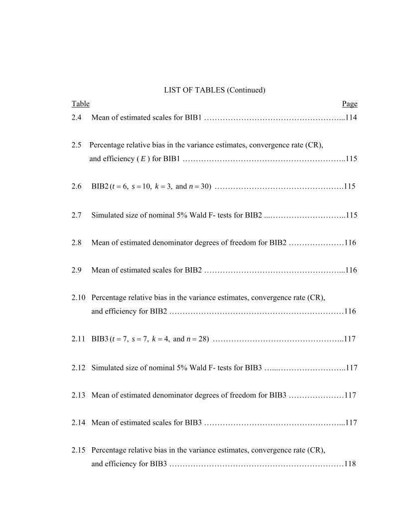
LIST OF TABLES (Continued)

Table Page

2.4 Mean of estimated scales for BIB1 ……………………………………………...114


and efficiency ( E ) for BIB1 ……………………………………………………..115

2.6 BIB2 ………………………………………….115 ( 6, 10, 3, and 30)t s k n= = = =





and efficiency for BIB2 …………………………………………………………116

2.11 BIB3 …………………………………………..117 ( 7, 7, 4, and 28)t s k n= = = =

2.12 Simulated size of nominal 5% Wald F- tests for BIB3 …...……………………..117




and efficiency for BIB3 …………………………………………………………118


Table Page

2.16 BIB4 ………………………………………….118 ( 9, 36, 2, and 72)t s k n= = = =





and efficiency ( E ) for BIB4 …………………………………………………….119

2.21 BIB5 design ( ………………………………….120 9, 18, 4, and 72)t s k n= = = =






2.26 BIB6 ………………………………………….121 ( 9, 12, 6, and 72)t s k n= = = =




Table Page




3.1 Simulated size of nominal 5% Wald F- tests for RCB1 ……..…………………122

3.2 Mean of estimated denominator degrees of freedom for RCB1 ………………...123

3.3 Mean of estimated scales for RCB1 ……………………………………………..123


and efficiency ( E ) for RCB1 …………………………………………………...123

3.5 Simulated size of nominal 5% Wald F- tests for RCB2 ..……………………….123

3.6 Mean of estimated denominator degrees of freedom for RCB2 ………………...124

3.7 Mean of estimated scales for RCB2 ……………………………………………..124


and efficiency ( E ) for RCB2 …………………………………………………...124

To my wife, Sohailah,

for her significant support.

KENWARD-ROGER APPROXIMATE F TEST FOR FIXED EFFECTS IN MIXED LINEAR MODELS

1. INTRODUCTION

When testing fixed effects in a mixed linear model, an exact F test may not exist.

Several approaches are available to perform approximate F tests, and one of the most

common approaches is the method derived by Kenward and Roger (1997). Since the

Kenward-Roger method has been implemented in the MIXED procedure of the SAS

system, it has become well known and widely used. In this thesis, we investigate the

Kenward-Roger approach, and suggest two other modifications.

1.1 Previous Results

In testing a hypothesis about fixed effects, it is desirable to find an exact test. In

balanced mixed linear models, the standard Anova method leads to optimal exact F tests

for the fixed effects in most cases. In such models, Seifert (1979) showed that the

standard Anova F tests are uniformly most powerful invariant unbiased tests (UMPIU).

Rady (1986) studied the needed assumptions for the mixed linear model so that the

Anova method produces optimal exact F tests for the fixed effects. Seely and Rady

(1988) studied conditions where the random effects can be treated as fixed to construct an

exact F test for the fixed effects. VanLeeuwen (1998) introduced the concept of

error orthogonal (EO) designs. In models with EO structure, we have an exact F test for

certain standard hypotheses. Utlaut (2001) introduced the concept of simple error

orthogonal (SEO) designs, in which optimal exact F tests can be obtained. If a mixed

effects Anova model has a type of “partial balance” called b&r balanced (VanLeeuwen

, 1999), then it is SEO. A typical normal balanced Anova model is b&r balanced,

and therefore, has an optimal exact F test as indicated above. In particular, when the

smallest random effect that contains a fixed effect is unique, there is an optimal exact F

test for the fixed effect which coincides with the Anova F test (Birkes, 2004). In addition,

exact F tests have been constructed for certain other models. For instance, an exact F test

.et al

.et al

.et al

2

can be obtained for testing certain hypotheses about fixed effects in a general multivariate

model (Mardia , 1992). Also, an exact F test can be obtained to test fixed effects in

a balanced multivariate model with a random group effect (Birkes, 2006).

.et al

In many cases, constructing an exact test seems hard and approximations need to

be employed. When no two mean squares in the Anova table have the same expectations

under the null hypothesis, the Anova method may still be used to obtain an approximate F

test. If a mean square can be created as a linear function of other mean squares such that

it has the same expectation as the mean square of the fixed effects under the null

hypothesis, then the created mean square is used in the denominator of an F test where its

degrees of freedom can be approximated by Satterthwaite (1946).

Another common approach to produce an approximate F test for the fixed effects

is based on the Wald-type statistic. When using a Wald-type test, the numerator degrees

of freedom equal the number of contrasts being tested, but the denominator degrees of

freedom needs to be estimated. In the Containment method, which is the default method

in SAS’s MIXED procedure, the denominator degrees of freedom are chosen be the

smallest rank contribution of the random effects that contain the fixed effects to the

design matrix. If no such effects are found, the estimate is the residual degrees of

freedom.

Giesbrecht and Burns (1985) proposed a method based on Satterthwaite (1941) to

determine the denominator degrees of freedom for an approximate Wald-type t test for a

single contrast of the fixed effects. Fai and Cornelius (1996) extended Giesbrecht and

Burns method where they approximate the Wald-type test for a multidimensional

hypothesis by an F distribution. Both approaches proposed by Giesbrecht and Burns, and

Fai and Cornelius use the conventional estimator of the variance-covariance matrix of the

fixed effects estimator, which is the variance-covariance matrix of the generalized least

squares (GLS) estimator of the fixed effects, replacing the variance components with the

REML estimates. The Fai and Cornelius approach is referred to as the Satterthwaite

approach in some literature and in this thesis as well. Bellavance (1996) suggested a

method to improve the Anova F test by using a scaled F distribution with modified

.et al

3

degrees of freedom.

It is known that the conventional estimator of the variance-covariance matrix of

the fixed effects estimator underestimates (Kackar and Harville, 1984). Indeed, Kackar

and Harville expressed the variance-covariance matrix of the fixed effects estimator as a

sum of two components. The first component is the variance-covariance matrix of the

GLS estimator of the fixed effects, and the second component represents what the first

component underestimates. The second component was approximated by Kackar and

Harville (1984) and Prasad and Rao (1990), and estimation of the first component was

addressed by Harville and Jeske (1992) and later by Kenward and Roger (1997). In fact,

Kenward and Roger (1997) combined estimators of the two components to produce an

adjusted estimator for the variance-covariance matrix of the fixed effects estimator. They

plug the adjusted estimator into the Wald-type statistic where a scaled form of the

statistic follows an F distribution approximately. Unlike the Satterthwaite-based

approaches where only the degrees of freedom need to be estimated, in Kenward and

Roger’s approximation, two quantities need to be estimated from the data: the

denominator degrees of freedom and the scaling factor.

After deriving approximate expressions for the expectation and the variance of the

Wald-type statistic, Kenward and Roger then match these with the first and second

moments of the F distribution to determine the estimates of the denominator degrees of

freedom and the scale. Moreover, Kenward and Roger modified the approximation in

such a way that the estimates match the known values for two special cases where a

scaled form of the Wald-type statistic has an exact F test. In fact, the idea of modifying

the approach in a way to produce the exact values was adopted previously by Graybill

and Wang (1980) when they modified approximate confidence intervals on certain

functions of the variance components in a way to make them exact for some special

cases.

Lately, the performance of Kenward and Roger’s approximation has become a

subject for some simulation studies. For example, Schaalje (2002) compared the K- .et al

R and the Satterthwaite approaches for a split plot design with repeated measures for

4

several sample sizes and covariance structures. They found that the K-R method performs

as well as or better than the Satterthwaite approach in all situations. They considered

three factors in the comparisons: the complexity of the covariance matrix, imbalance, and

the sample size, and they found that these factors affect the Satterthwaite method more

than the K-R method. The Satterthwaite method was found to work well only when the

sample size is moderately large and the covariance matrix was compound symmetric. The

K-R method was found to have a tendency toward inflated levels when the sample size

was small, except when the covariance structure was compound symmetric. Chen and

Wei (2003) compared the Kenward-Roger approach and a modified Anova method

suggested by Bellavance (1996) for some crossover designs. They recommended

using the K-R approach when the sample size is at least 24. For smaller sample sizes,

they found the modified Anova method works better than the K-R approach. Savin

(2003) found the K-R approach reliable to construct a confidence interval for the

common mean in interlaboratory trials. Spike (2004) investigated the K-R and the

Satterthwaite methods to estimate the denominator degrees of freedom for contrasts of

the fixed subplot effects. Like the conclusion drawn by Schaalje (2002) above, they

suggested Kenward and Roger’s approximation be preferred in small datasets, and the

two methods are comparable for large datasets. Valderas (2005) studied the

performance of the K-R approach when AIC and BIC are used as criteria to select the

covariance structure. They found the K-R method’s level much higher than the target

values. Even with the correct covariance structure, the level was found to be higher than

the target for many cases in which the covariance structure is not compound symmetric.

.et al

.et al

.et al

.et al

.et al

1.2 Contributions and Summary of Results

Since some of the detailed derivation for Kenward and Roger’s approach was

absent from their original work, we provide the detailed theoretical derivation of the

method which includes clarifying the assumptions to justify the theoretical derivation.

Also, we weaken some of the assumptions that were imposed by Kenward and Roger,

and determine the orders of the approximations used in the derivation. We present two

5

modifications of the K-R method which are comparable in performance but simpler in

derivation and computation. Kenward and Roger modified their approach in such a way

that their method reproduces exact F tests in two special cases, namely for Hotelling

and for Anova F ratios. We show that the K-R and the two proposed methods reproduce

exact F tests in three more general models, two of which are generalizations of the two

special cases. We explore relationships among the K-R, proposed and Satterthwaite

methods by specifying cases where the approaches produce the same estimate of the

denominator degrees of freedom or are even identical. Also, we show the difficulties in

developing a K-R type method using the conventional, rather than adjusted, estimator of

the variance-covariance matrix of the fixed-effects estimator.

2T

In chapter 2, using Taylor series expansions, matrix derivatives and invariance

arguments, we derive the adjusted estimator for the variance -covariance matrix of the

fixed effects estimator that was provided by Kenward and Roger (1997). Besides

clarifying all assumptions that justify the theoretical derivation, we weaken some of the

assumptions imposed by Kenward and Roger. In addition, we determine the orders of the

approximations used in the derivation.

In chapter 3, we derive the approximate expectation and variance of the Wald-

type statistics where they are constructed by using the conventional and the adjusted

estimator of the variance-covariance matrix of the fixed effects estimator. In addition, we

match the first and second moments of F distribution with these for the scaled form of the

Wald-type statistic to obtain the Kenward-Roger approximation for the denominator

degrees of freedom and scale before the modification.

Two special cases: the balanced one-way Anova model, and the Hotelling

model where the Wald-type statistic have an exact F distribution are considered in

chapter 4 to establish the modification of the expectation and the variance of the Wald-

type statistic proposed by Kenward and Roger so the approach produces the right and

known values for these two special cases. Kenward and Roger (1997) mentioned that it

can be argued that the conventional estimator of the variance-covariance matrix of the

fixed effects estimator can be used instead of the adjusted estimator. We discuss the

2T

6

difficulties in modifying the approach by using the conventional estimator instead of the

adjusted estimator.

The K-R approach was derived based on modifying the approximated expressions

for the expectation and the variance of the Wald-type statistic. This modification is not

unique, and hence we introduce two other modifications for the K-R method in chapter 5.

We keep the modification of the expectation of the statistic as modified by Kenward and

Roger; however, instead of modifying the variance, we modify other related quantities.

The proposed modifications for the K-R method are comparable in performance and

simpler in derivation and computation.

As mentioned above, the special cases used by Kenward and Roger are not the

only cases where the K-R and proposed methods produce the exact values. Indeed, the

Kenward-Roger and the proposed modifications produce the exact values for three

general models where there is an optimal exact F test. The models studied in chapter 6

are: (1) Rady’s model (with a slight modification) which includes a wide class of

balanced mixed classification models and is more general than the balanced one-way

Anova model, (2) a general linear multivariate model which is more general than the

Hotelling , and (3) a balanced multivariate model with a random group effect. We

show that the estimate of the denominator degrees of freedom and the scale factor match

the known values for those models.

2T

The Satterthwaite, the Kenward-Roger and the proposed methods perform

similarly in some situations. Chapter 7 is devoted to study the cases where these methods

produce the same estimate for the denominator degrees of freedom. Moreover, we study

the cases where the approaches become identical to each other.

In chapter 8, we provide a simulation study for three types of block designs:

partially balanced incomplete block designs, balanced incomplete block designs and

complete block designs with some missing data. In the simulation study, the sample size,

the ratio of the variance components, and the efficiency factor are considered to see how

they affect the performance of the Kenward-Roger, the proposed, the Satterthwaite and

the Containment methods.

7

2. VARIANCE-COVARIANCE MATRIX OF THE FIXED EFFECTS ESTIMATOR

For a multivariate mixed linear model, statisticians used to estimate the precision

of the fixed effects estimates based on the asymptotic distribution. However, this estimate

was known to be biased and underestimate the variance of the fixed effects estimate.

Kenward and Roger (1997) proposed an adjustment for the estimator of the variance of

the fixed effects estimator which is investigated in this chapter.

2.1 The Model

Consider observations following a multivariate normal distribution,n y

y N , (Χβ,Σ)∼

where is a full column rank matrix of known covariates, is a vector of

unknown parameters and

(n p×Χ ) )

)

( 1p×β

(n n×Σ is an unknown variance-covariance matrix whose

elements are assumed to be functions of parameters, r 1( 1) ( ,...., )rr σ σ ′× =σ . The

generalized least squares estimator of is , and the matrix

is the variance-covariance matrix of this estimator. The REML

estimator of is denoted by , and the REML-based estimated generalized least squares

estimator of (EGLSE) is . The center of our study isβ , and

is a nuisance to be addressed in the analysis. We are interested in testing

β 1 1 1( )− − −′ ′=β Χ Σ Χ Χ Σ y1( − −′= 1Φ ΧΣ Χ)

ˆ )

σ σ

β 1 1 1ˆ ˆ( ( ) ) (− − −′ ′=β Χ Σ σ Χ Χ Σ σ y

Σ 0H : ′ =L 0β ,

for . an ( ) fixed matrixp′ ×L

2.2 Notation

Throughout the thesis, we use the following notation. For a matrix , we use A

, ( ), ), r( ), tr( ), ,′ ℜA A A A A AN( to denote transpose, range, null space, rank, trace,

and determinant of respectively. A ( )⊥ℜ A is used to denote the orthogonal complement

of We use the abbreviation p.d. for positive definite and n.n.d. for nonnegative

definite. The notation p.o. is used for projection operator and o.p.o. for orthogonal

( ).ℜ A

8

projection operator. is o.p.o. onAΡ ( )ℜ A . In addition, we use the following

1 1 1 1 1

1

1

1 1

1 1 1

21 1

1 1

A

ˆVar( )ˆ ˆ ˆVar( ), Cov( , )

( )( )

( )

ˆVar( )

( )

ˆ

ij i j

ii

iji j

iji j

r r

ij ij i ji j

w

w

σ σ

σ

σ σ

σ σ

− − − − −

−

− −

− −

− − −

− −

= =

== =

′ ′= −

′ ′=

′=∂′= −∂

∂ ∂′=∂ ∂

∂′=∂ ∂

= −

= −

=

∑∑

1

V βW σ

G Σ Σ Χ ΧΣ Χ ΧΣΘ L L ΦL LΦ ΧΣ Χ

ΣΡ Χ Σ Σ Χ

Σ ΣQ ΧΣ Σ Σ Χ

ΣR ΧΣ Σ Χ

Λ β β

Λ Φ Q Ρ ΦΡ Φ

Φ1 1

11 1

21 1

31 1

1A

1ˆˆ ˆ ˆ ˆ ˆ ˆ ˆˆ2 ( )4

tr( )tr( )

tr( ),

1tr[ ( ) ]4

1 ˆ ˆˆ( ) , unless otherwise

r r

ij ij i j iji j

r r

ij i ji j

r r

ij i ji j

r r

ij ij i j iji j

w

A w

A w

A w

F

= =

= =

= =

= =

−

⎧ ⎫+ − −⎨ ⎬

⎩ ⎭

=

=

= − −

′ ′ ′=

∑∑

∑∑

∑∑

∑∑

Φ Φ Q Ρ ΦΡ R Φ

ΘΦΡ Φ ΘΦΡ Φ

ΘΦΡ ΦΘΦΡ Φ

ΘΦ Q Ρ ΦΡ R Φ

β L L Φ L L β mentioned.

ˆ ˆFor a matrix ( ), we use ( ).=H σ H H σ

2.3 Assumptions

For chapters 2 and 3, we impose the following assumptions about the model.

(A1) The expectation of exists. β

(A2) is a block diagonal and nonsingular matrix. Also, we assume that the elements of Σ

9

21, , , , and k k

k k ki i jσ σ σ

− ∂ ∂∂ ∂ ∂Σ ΣΣ Σ Χ are bounded, where 1diag ( ), andk m k≤ ≤=Σ Σ

1col ( ),

k m k≤ ≤=Χ Χ and sup , where are the blocks sizes. in < ∞ in

(A3) 32Ê[ ] ( ).O n−= +σ σ .

(A4) The possible dependence between is ignored. ˆˆ and σ β

52

r

1 1

ˆ ˆ(A5) Cov ( )( ) , ( )( ) ( ).r

i i j ji j i j

O nσ σ σ σσ σ

−

= =

⎡ ⎤∂ ∂ ′ − − =⎢ ⎥∂ ∂⎢ ⎥⎣ ⎦

∑∑ β β

(A6) 1 12 2

21 1 1

2( ) ( ), ( ) ( ), ( ), ( )i i

O n O n O n O nσ σ

− −− − − − ∂ ∂′ ′= = = = =∂ ∂

1 β βΦ ΧΣ Χ L ΦL

(A7) If ( ), then E[ ] ( )pO n O nα α= =T T

Remarks

( )i kΣ is said to be bounded when max (elements of ) ( )k b≤Σ σ for some constant b .

Since , then sup in < ∞ .n m→∞⇔ →∞

( )ii Even though Kenward and Roger required the bias of the REML estimator to be

ignored, we only require 32Ê[ ] ( )O n−= +σ σ as stated as assumption (A3). In fact, for the

model mentioned in section 2.1, is of order 2Ê[ ] ( ) ( ), where ( )O n−− = +σ σ b σ b σ 1( )O n−

(Pase and Salvan, 1997, expression 9.62). Moreover, when the covariance structure is

linear, , and hence which is stronger than what we need. ( ) =b σ 0 2Ê[ ] ( )O n−− =σ σ

( )iii Assumption (A4) was also imposed by Kenward and Roger. In fact, we did

investigate some models, like Hotelling model, the fixed effects model, and the one

way Anova model with fixed group effects and unequal group variances. In these models,

are independent exactly. Also, for those models, the sum of covariance in

assumption (A5) is zero which is stronger than the assumption. This assumption is

needed to derive approximate expressions for the expectation and the variance of the

statistic by conditioning on as we will see in chapter 3. However, we should mention

2T

ˆˆ and σ β

σ

10

that the same derivation of the expectation and the variance of the statistic can be done

without conditioning on , in which case assumption (A4) is not needed anymore. σ

( )iv One circumstance for the covariance in assumption (A5) to be exactly zero is

when is obtained from a previous sample, and from current data (Kackar and

Harville, 1984). Also, Kackar and Harville argued that when is unbiased and

σ ( )β σ

σ

ˆE ( )( ) |i jσ σ

⎡ ⎤∂ ∂ ′⎢∂ ∂⎢ ⎥⎣ ⎦

β β σ⎥ can be approximated by first order Taylor series, then the covariance

in (A5) is expected to be zero. It appears that Kenward and Roger assumed one of the

arguments mentioned. For us, it is enough to assume (A5).

1

21

( ) ( ) ( ), where ( ) diag ( ( ), and ( ) is a product of any

combination of , , , and . This is true because ( ) (1)

for 1 max(elements of ( ) ) f

k m k k

k kk k k k k

i i j

k k k

v O n

O

k m a

σ σ σ

≤ ≤

−

′ = =

∂ ∂ ′ =∂ ∂ ∂

′≤ ≤ ⇒ ≤

ΧH σ Χ H σ H σ H σ

Σ ΣΣ Σ Χ H σ Χ

Χ H σ Χ

1

1 1

1

or 1

max(elements of ( ) )

max(elements of ( ) ) max(elements of ( ) ) ,

and hence ( ) ( ) ( ) ( ).

m

k k kk

m m

k k k k k kk k

m

k k kk

k m

ma

ma

O m O n

=

= =

=

≤ ≤

′⇒ ≤

′ ′⇒ ≤

′ ′= = =

∑

∑ ∑

∑

Χ H σ Χ

Χ H σ Χ Χ H σ Χ

ΧH σ Χ Χ H σ Χ

≤

( )vi A general situation where the first two conditions in assumption (A6) hold is when

all are contained in a compact

set

1k k k

−′Χ Σ Χ

1 11 of p.d. matrices mm

− −′⇒ ∈ ⇒ ∈ΧΣ Χ Φ

1− =

1 1and hence ( ). Also, we have (p.d.) ( ) ( ).O n m O n− −′ ′ ′= ∈ ⇒Φ L ΦL L L L ΦL

Also, this assumption holds when we suppose 1k k= ∀Σ Σ , and we suppose that

11

1

1 (p.d.).m

k kkm

−

=

′ →∑Χ Σ Χ A This supposition is reasonable in two situations:

11 11) , and in this case, .k k −′= ∀ =Χ Χ A Χ Σ Χ1 1

2) are regarded as iid random covariate matrices, and by the weak law of large numbers,kΧ

11

1 11 1 1 1

1 1

1 1 1 1

1

converges to E[ ].

Then, since inversion is a continuous operation, . That is ( )1Also, ( ) ( ) . That is ( ) ( ).

(as we will see

k k

i i

m O

O nm

σ σ

− −

− −

− − − −

−

′ ′

→ =

′ ′ ′→ =

∂ ∂′= −∂ ∂

Χ Σ Χ Χ Σ Χ

Φ A Φ

L ΦL L A L L ΦL

β ΣΦΧΣ Gy

n

1

1

1

1

in lemma 2.4.7).

Consider ( ) , where ( ) , and ( ) ( ) ,

where col ( ), and ( ) diag ( ( ). If ( ) are iid, then by the

weak law of large numbers, we ha

k m

m

k k kki

k m k k k k k

σ

≤ ≤

−

=

≤ ≤

∂′ ′= =∂

′= =

∑ΣΧ B σ y B σ Σ G Χ B σ y Χ B σ y

y y B σ B σ Χ B σ y

′

1

1ve ( ) E[ ( ) ] (1).m

k k k k k kk

m Om =

⎡ ⎤′ ′− =⎢ ⎥⎣ ⎦∑Χ B σ y Χ B σ y

12

1 12 21

However, in lemma (2.4.7), we have E[ ( ) ] , and hence ( ) ( ).

( ) ( ) ( ).

ˆ( ) If ( ) ( ), then ( ) ( ). This result is obtained by employing a Taylor

series

k k k

i

p p

O n

O n O n O n

vii O n O nα α

σ−−

′ ′= =

∂⇒ = =

∂

= =

Χ B σ y 0 ΧB σ y

β

H σ H σ

32

ˆexpansion for ( ) about . ( ) For some random matrices , their expectations have higher order than the random

ˆ ˆ ˆmatrices themselves. For instance, ( )( )( ) ( ), as it will be

si i j j k k p

viii

O nσ σ σ σ σ σ −− − − =

H σ σT

2ˆ ˆ ˆhown in theorem (2.4.9); however, E[( )( )( )] ( ), fromi i j j k k O nσ σ σ σ σ σ −− − − =

expression (9.74) in Pace and Salvan. In assumption (A7), we assume that the expectation

will reserve the order which does not conflict with the cases mentioned above.

2.4 Estimating Var( ) β

There are two main sources of bias in when it is used as an estimator for

Var( ): underestimates , and does not take into account the variability of

in . Kackar and Harville (1984) proposed that Var( ) can be partitioned as

Var( ) = , and they addressed the second source of bias by approximating .

The first source of bias was discussed by Harville and Jeske (1992), and Kenward and

Roger (1997) proposed an approximation to adjust the first bias, and they combined both

Φ

β Φ Φ Var( )=Φ β

σ ˆ ˆ( )=β β σ β

β +Φ Λ Λ

12

adjustments to calculate their proposed estimator of Var( ) which is denoted by . In

this section, several lemmas are derived to lead to the expression for .

β AΦ

AΦ

Lemma 2.4.1 With ( ) being the likelihood function of , where ,RL ′ ′ =σ z = Κ y ΚΧ 0

-1

With ( ) being the likelihood function of , where ,

2log ( ) 2 ( ) constant log logR

R R

L

L

′ ′ =

′= = − −

σ z = Κ y Κ Χ 0

σ σ Σ Χ Σ Χ

1 1 -1 1 1( )− − − −′ ′ ′⎡ ⎤− −⎣ ⎦y Σ Σ Χ Χ Σ Χ Χ Σ y

Proof 1

2 2 1N , ( ) (2 ) exp ( ) ( )2

nf π − − −⎡ ⎤′= − − −⎢ ⎥⎣ ⎦

1y (Χβ,Σ) y Σ y Χβ Σ y Χβ∼

, (Birkes, 2004, theorem 7.2.2). N ′z (0,Κ ΣΚ)∼

and 1 12 2 1( ) (2 ) exp ( )

2

qf π − − −⎡ ⎤′ ′ ′= −⎢ ⎥⎣ ⎦

z Κ ΣΚ z Κ ΣΚ z , where q n p= − .

The REML estimator for is the maximum likelihood estimator from the marginal

likelihood of where

σ

′z = Κ y ′Κ is any q n× matrix of full column rank

1

1

2 ( ) log(2 ) log( ) ( )

log(2 ) log( ) ( )R q

q

π

π

−

−

′ ′ ′= − − −

′ ′ ′ ′= − − −

σ Κ ΣΚ z Κ ΣΚ z

Κ ΣΚ y Κ ΚΣΚ Κ y

To prove the lemma, it suffices to show that 1 1 1 1 1 1

1

( ) ( ) ( )

( ) log(2 ) log constant log log

a

b q π

− − − − − −

−

′ ′ ′ ′ ′ ′⎡ ⎤= −⎣ ⎦′ ′− − = − −

y Κ Κ ΣΚ Κ y y Σ Σ Χ ΧΣ Χ ΧΣ y

Κ ΣΚ Σ Χ Σ Χ

For part ( ), it suffices to show that a

1 1 1 -1 1( ) ( )− − − −′ ′ ′ ′= −Κ Κ ΣΚ Κ Σ Σ Χ ΧΣ Χ ΧΣ 1−

1 1 -1 1

1 1 1 -1 1 1

Indeed, ( ) ( ) (Seely, 2002, problem (2.B.4)) ( ) ( )

− − −

− − − − −

′ ′ ′ ′= −

′ ′ ′ ′⇒ = −

Κ Κ ΣΚ Κ Σ Ι Σ Χ ΧΣ Χ ΧΚ Κ ΣΚ Κ Σ Σ Χ ΧΣ Χ ΧΣ

Observe that is nonsingular (assumption A2), and n.n.d (Birkes, 2004), then is p.d. (Seely, 2002, corollary 1.9.3), and hence r( ) r( ) (Birkes, 2004, a lemma on Jan 23).′ ′=

Σ Σ

Κ ΣΚ Κ

Also,we have ( ) ( ) (because ( ) ( ) )⊥′ℜ = ℜ =ℜΚ Χ Κ ΧN

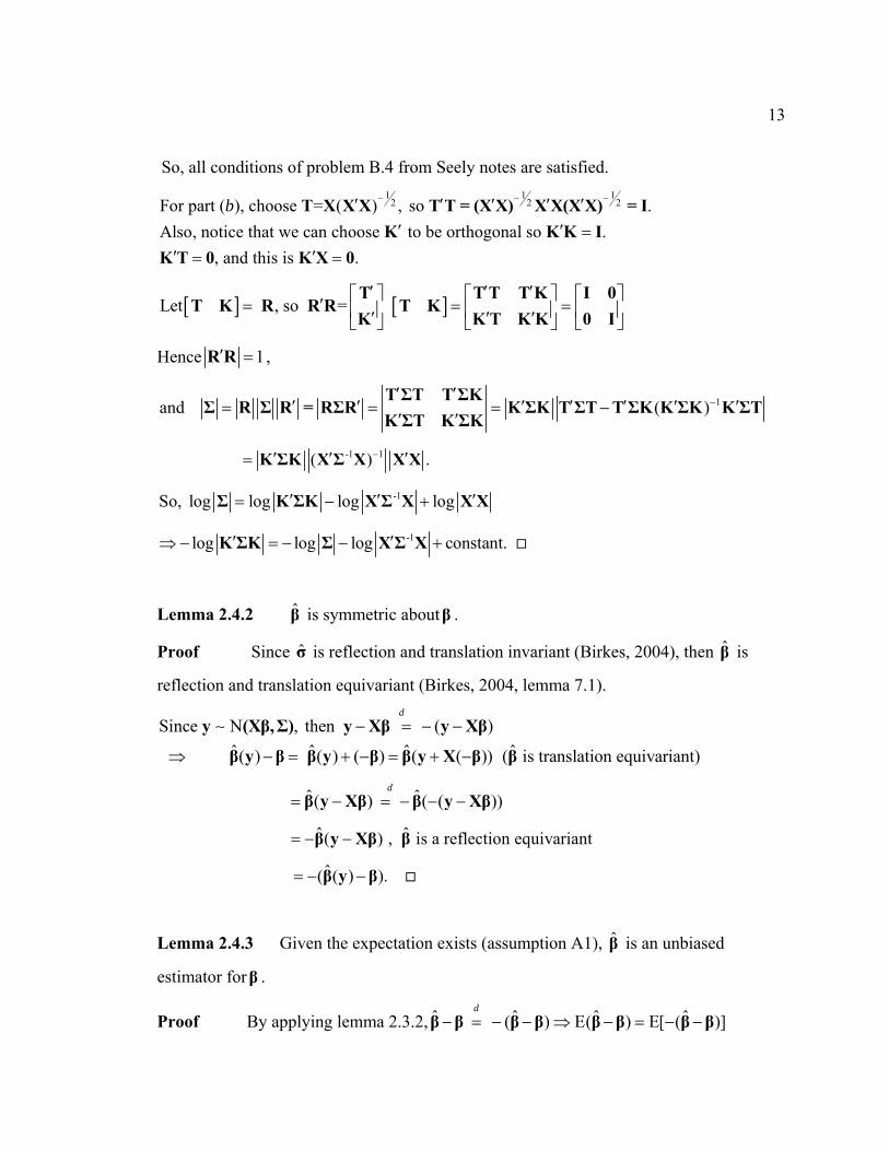
13

So, all conditions of problem B.4 from Seely notes are satisfied. 1 1

2 2For part ( ), choose = ( ) , so .Also, notice that we can choose to be orthogonal so .

, and this is .

b − −′ ′ ′ ′ ′′ ′ =

′ ′= =

Τ Χ ΧΧ Τ Τ = (ΧΧ) ΧΧ(ΧΧ) = ΙΚ Κ Κ

Κ Τ 0 Κ Χ 0

12−

Ι

[ ] [ ]Let , so = ′ ′ ′⎡ ⎤ ⎡ ⎤ ⎡ ⎤′= =⎢ ⎥ ⎢ ⎥ ⎢ ⎥′ ′ ′⎣ ⎦ ⎣ ⎦ ⎣ ⎦

Τ Τ Τ Τ Κ 0Τ Κ R R R Τ Κ

Κ Κ Τ ΚΚ 0 Ι=

Ι

Hence 1′ =R R ,

1and ( )−′ ′

′ ′ ′ ′ ′ ′ ′= = = −′ ′

Τ ΣΤ Τ ΣΚΣ R Σ R = RΣR Κ ΣΚ Τ ΣΤ Τ ΣΚ Κ ΣΚ Κ ΣΤ

Κ ΣΤ Κ ΣΚ

-1 1 ( ) .−′ ′ ′= Κ ΣΚ Χ Σ Χ ΧΧ

-1So, log log log log′ ′= − +Σ Κ ΣΚ ΧΣ Χ Χ′Χ

-1log log log constant. ′ ′⇒ − = − − +Κ ΣΚ Σ ΧΣ Χ

Lemma 2.4.2 is symmetric aboutβ . β

Proof Since is reflection and translation invariant (Birkes, 2004), then is

reflection and translation equivariant (Birkes, 2004, lemma 7.1).

σ β

Since N , then ( )ˆ ˆ ˆ ˆ ( ) ( ) ( ) ( ( )) ( is translation equivariant)

d− = − −

⇒ − = + − = + −

y (Χβ,Σ) y Χβ y Χβ

β y β β y β β y Χ β β

∼

ˆ ˆ ( ) ( ( ))d

= − = − − −β y Χβ β y Χβ

ˆ ˆ ( ) , is a reflection equivariant= − −β y Χβ β

ˆ ( ( ) ). = − −β y β

Lemma 2.4.3 Given the expectation exists (assumption A1), is an unbiased

estimator for .

β

β

Proof By applying lemma 2.3.2, ˆ ˆ ˆ ˆ ( ) E( ) E[ (d

)]− = − − ⇒ − = − −β β β β β β β β

14

ˆ ˆ ˆ ˆE( ) E( ) 2E( ) 2 E( ) . ⇒ − = − + ⇒ = ⇒ =β β β β β β β β

Lemma 2.4.4 are independent. and ( )Χβ Ι -Ρ y

Proof 1 1 1Cov , Cov ( ) , ( )− − −⎡ ⎤ ′ ′⎡ ⎤= ⎣ ⎦⎣ ⎦Χ Χβ (Ι -Ρ )y Χ Σ Χ Χ Σ y Ι -Ρ y

1 1 1 1 1

1 1 -1 1

1 1 1 1

( ) ( ) ( ) ( )

( ) ( )

( ) ( )

− − − − −

− − −

− − − −

′ ′ ′ ′= =

′ ′ ′ ′= −

′ ′ ′ ′= − =

Χ Χ

Χ

Χ Σ Χ ΧΣ Σ Ι -Ρ Χ Σ Χ Χ Ι -Ρ

Χ Σ Χ Χ ΧΣ Χ Χ Ρ

ΧΣ Χ Χ ΧΣ Χ Χ 0

Since are both normally distributed, then they are independent (Birkes,

2004, proposition 7.2.3).

and ( )Χβ Ι -Ρ y

Lemma 2.4.5 . ˆ is a function of ( )− Χβ β Ι -Ρ y

Proof ˆConsider ( )( ) ( ), and hence ( ) is a translation-invariant function.− =β β y δ y δ y

(1) (2) (1) (2)

(1) (2) (1) (1) (2) (2)

(2) (1) (1)

To show that ( ) is a function of ( ) , it is equivalent to show that:

( ) ( ) ( ) ( )

( ) ( )

= ⇒ =

= ⇒ − = −

⇒ = − +

Χ

Χ Χ

Χ Χ Χ Χ

Χ Χ

δ y Ι -Ρ y

Ι -Ρ y Ι -Ρ y δ y δ y

Ι -Ρ y Ι -Ρ y y Ρ y y Ρ y

y y Ρ y Ρ (2) (1) (2) (1)

(2) (1)

1

( )

( ) ( ) for some ( is translation invariant).

= + −

⇒ = +

=

Χ

( )

y y Ρ y y

δ y δ y Χb bδ(y ) δ

Lemma 2.4.6 ˆ ˆVar( ) , where Var( )= + = −β Φ Λ Λ β β

Proof From lemma 2.4.4, are independent, and from lemma 2.4.5,

is a function of (

and ( )Χβ Ι -Ρ y

ˆ −β β )ΧΙ -Ρ y . Then, and β ˆ −β β are independent.

ˆ ˆWrite ˆ ˆ Var( ) Var( ) Var( ) .

= + −

⇒ = + − = +

β β β β

β β β β Φ Λ

15

Lemma 2.4.7 ˆE , and E ( )( ) for 1,....,i ii i

i rσ σσ σ

⎡ ⎤ ⎡ ⎤∂ ∂= − =⎢ ⎥ ⎢ ⎥∂ ∂⎣ ⎦ ⎣ ⎦

β β0 0 = .

Proof 1 1( )i iσ σ

− − −∂ ∂ ′ ′⎡ ⎤= ⎣ ⎦∂ ∂1β Χ Σ Χ ΧΣ y

1 1 1 1 ( ) ( ) i iσ σ

− − − −∂ ∂′ ′ ′ ′⎡ ⎤ ⎡= +⎣ ⎦ ⎣∂ ∂-1 -1ΧΣ Χ ΧΣ y ΧΣ Χ ΧΣ y⎤⎦

1 1 1 -1 1 1 where ( ) (2.1)iσ

− − − − −∂′ ′= − = −∂ΣΦΧΣ Gy G Σ Σ Χ ΧΣ Χ ΧΣ′

1 1E E E(i iσ σ σ

− −⎡ ⎤ ⎡ ⎤∂ ∂ ∂′ ′⇒ = − = −⎢ ⎥ ⎢ ⎥∂ ∂ ∂⎣ ⎦⎣ ⎦

β ΣΦΧΣ G )i

Σy ΦΧΣ Gy ,

1 1 -1 1 1

1 -1 1 -1 1

where [ ] E[( ( ) ) ] E[ ( ) ] ( ) .

− − − −

− − −

′ ′Ε = −

′ ′= − = − =

Gy Σ Σ Χ ΧΣ Χ ΧΣ yΣ y Χ ΧΣ Χ ΧΣ Y Σ Χβ Χβ 0

1ˆ ˆE ( ) [ ( )], where ( ) ( ( ) ).i i i ii i

g gσ σ σσ σ

−⎡ ⎤∂ ∂′− = − Ε = −⎢ ⎥∂ ∂⎣ ⎦

β ΣΦΧΣ y y Gy y σ

[ ] [ ]ˆ ˆ ˆ( ) ( ) ( ) ) ( ) ) ( ), because is reflection equivariant. So, is reflection-equaivariant.

i i i i ig ggσ σ σ σ σ− = − − − = − − − = −y G y y Gy y y

Since N

( ) 2

and hence g( ) g( 2 )

d d

d

⇒ − = − − ⇒ = − +

= − +

y (Χβ,Σ)

y Χβ y Χβ y y Χβ

y y Χβ

∼

g[ ( 2 )] because is reflection equivariantg= − + −y Χ β

( ), because is translation invariant.g g= − y

[ ]ˆNotice that ( ) ( ) ( )i ig σ σ+ = + + −y Χβ G y Χβ y Χβ

[ ]ˆ ˆ ( ) ( ) [ ( ) ] ( ),i i i i gσ σ σ σ= + + − = − =Gy GΧβ y Χβ Gy y y

and hence is a translation invariant function.g

Since ( ) ( ), then [ ( )] [ ( )] [ ( )]

ˆ2 [ ( )] [ ( )] , and hence E ( )( ) for 1,...., i ii

g g g g g

g g iσ σσ

= − Ε = Ε − = −Ε

⎡ ⎤∂⇒ Ε = ⇒ Ε = − = =⎢ ⎥∂⎣ ⎦

y y y y y

βy 0 y 0 0 r

16

Lemma 2.4.8 ( ) ii

aσ∂

= −∂Φ ΦΡ Φ

2

1 1 1 1 1

21 1

( ) ( ) ,

where , ,

and

i j j i ij ji iji j

i iji i

iji j

bσ σ

σ σ

σ σ

− − − − −

− −

∂= + − − +

∂ ∂

∂ ∂′ ′= − =∂ ∂

∂′=∂ ∂

Φ Φ Ρ ΦΡ Ρ ΦΡ Q Q R Φ

Σ ΣΡ Χ Σ Σ Χ Q ΧΣ Σ Σ Χ

ΣR ΧΣ Σ Χ

jσ∂∂Σ

Proof 1

-1 1 1 1( )( ) ( ) ( )i i

aσ σ

−− − −′∂ ∂′ ′= −

∂ ∂Φ ΧΣ ΧΧΣ Χ ΧΣ Χ

1

1 1 1 1( ) ( ) iiσ

−− − − −∂′ ′ ′= − = −

∂ΣΧΣ Χ Χ Χ ΧΣ Χ ΦΡΦ,

2 1

1 1 1 1( ) ( ) ( )i j i j

bσ σ σ σ

−− − − −

⎧ ⎫∂ ∂ ∂⎪ ⎪′ ′ ′= − ⎨ ⎬∂ ∂ ∂ ∂⎪ ⎪⎩ ⎭

Φ ΣΧ Σ Χ Χ Χ ΧΣ Χ

1 11 1 1 1 1 1

2 11 1 1 1

( ) ( ) ( )

( ) ( )

i j

i j

σ σ

σ σ

− −− − − − −

−− − − −

∂ ∂′ ′ ′ ′ ′=∂ ∂

∂′ ′ ′−∂ ∂

Σ ΣΧ Σ Χ Χ Χ ΧΣ Χ Χ Χ ΧΣ Χ

ΣΧΣ Χ Χ Χ ΧΣ Χ

−

1 11 1 -1 1 -1 1

2 1

( ) ( ) ( )

.

j i

i j j ii j

σ σ

σ σ

− −− − − −

−

∂ ∂′ ′ ′ ′ ′+∂ ∂

⎧ ⎫∂⎪ ⎪′= − +⎨ ⎬∂ ∂⎪ ⎪⎩ ⎭

Σ ΣΧ Σ Χ Χ Χ ΧΣ Χ Χ Χ ΧΣ Χ

ΣΦ Ρ ΦΡ Χ Χ Ρ ΦΡ Φ (2.2)

Observe that 2 1

1 1

i j i jσ σ σ σ

−− −

⎛ ⎞∂ ∂ ∂′ ′= −⎜ ⎟⎜ ⎟∂ ∂ ∂ ∂⎝ ⎠

Σ ΣΧ Χ Χ Σ Σ Χ

21 1 1 1 1 1 1 1

i j i j j iσ σ σ σ σ σ− − − − − − − −∂ ∂ ∂ ∂ ∂′ ′ ′= − +∂ ∂ ∂ ∂ ∂ ∂Σ Σ Σ Σ ΣΧ Σ Σ Σ Χ Χ Σ Σ Χ Χ Σ Σ Σ Χ

(2.3)ij ij ji= − +Q R Q

Combining expressions 2.3 and 2.3, we obtain

17

2

( ) i j j i ij ji iji jσ σ∂

= + − − +∂ ∂

Φ Φ Ρ ΦΡ Ρ ΦΡ Q Q R Φ.

=

Before proceeding, we present asymptotic orders for some terms that will be used often

in chapters 2 and 3.

Lemma 2.4.9 1( ) ( ), ( ) ( ), ( ) ( ), ( ) ( ),i ij ija O n b O n c O n d O n−= = =Φ Ρ Q R

1 2

221 1 2

2

22

ˆ ˆ( ) ( ), ( ) Cov( , ) ( ), ( ) ( ), ( ) ( ),

( ) ( ), ( ) ( ), ( ) ( ), ( ) ( ),

ˆ( ) ( ), ( ) (

ij i ji

ij ij

i j i i i

i i pi

e O n f w O n g O n h O n

w wi O n j O n k O n l O n

m O n n O n

σ σσ

σ σ σ σ σ

σ σσ

− −

− − −

−

∂= = = = =

∂

∂ ∂∂ ∂= = = =

∂ ∂ ∂ ∂ ∂

∂= − =

∂

ΦΘ Λ

Φ Λ

Λ

1

1

−

−

12 )−

Proof Parts ( ), ( ), and( ) are direct from remark( ) above.b c d v

Parts ( and( e ) are direct from assumption (A6). )a

1

2

( ), where is the ( , ) entry of the inverse of the expected information matrix

(Pace and Salvan, 1997, expression 9.73). Pace and Salvan, showed that ( ),and ( ) ( ).

From parts

ij ijij

ij

w i a i i j

i O na O n

−

−

= +

=

=

σ

σ2

2

( ), ( ), ( ), and ( ), we have ( ).

Since , ( ) (lemma 2.4.8 ),

then from previous parts, results ( ) and ( ) are obtained.

By using expression (9.17) i

i i j j i ij ji iji i j

a b c f O n

h i

σ σ σ

−=

∂ ∂= − = + − − +

∂ ∂ ∂

ΛΦ ΦΦΡ Φ Φ Ρ ΦΡ Ρ ΦΡ Q Q R Φ

1

2 21 2 2

2 2

n Pace and Salvan(1997), we have ( ),

( ) ( )( ), ( ), and ( )hence results ( ) and ( ) are

obtained. By computing the derivative of , and using previous par

ij

iij

i i i

i O n

i a aO n O n O n j l

σ

σ σ σ

−

− − −

∂=

∂

∂ ∂ ∂= = =

∂ ∂ ∂σ σ

Λ ts, results ( )and ( ) are obtained. Finally, expression ( ) is a direct result of the asymptotic normality

ˆof ( ) (Pace and Salvan, expression 3.38). i i

km n

n σ σ−

18

Lemma 2.4.10 52ˆVar( ) ( ),O n−= − = +Λ β β Λ

Proof Using a Taylor series expansion aboutσ , we have

32

32

3 32 2

1

1

1 1

ˆ ˆ ˆ ( ) ( ) ( ) ( ).

ˆ ˆ ( ) ( ),

ˆ ˆ ˆand Var( ) E ( ) ( ) ( ) ( )

r

i i pi i

r

i i pi i

r r

i i p i i pi ii i

O n

O n

O n O n

σ σσ

σ σσ

σ σ σ σσ σ

−

=

−

=

− −

= =

∂= = + − +

∂

∂⇒ − = − +

∂

⎡ ⎤′⎛ ⎞⎛ ⎞∂ ∂⎢ ⎥= − = − + − +⎜ ⎟⎜ ⎟⎢ ⎥∂ ∂⎝ ⎠⎝ ⎠⎣ ⎦

∑

∑

∑ ∑

ββ β σ β σ

ββ β

β βΛ β β

3 32 2

1 1

ˆ ˆ E ( ) ( ) E ( ) ( )r r

i i p i i pi ii i

O n O nσ σ σ σσ σ

− −

= =

′⎡ ⎤ ⎡ ⎤⎛ ⎞ ⎛ ⎞∂ ∂− − + − +⎢ ⎥ ⎢ ⎥⎜ ⎟ ⎜ ⎟∂ ∂⎝ ⎠ ⎝ ⎠⎣ ⎦ ⎣ ⎦

∑ ∑β β

Applying lemma 2.4.7, we obtain

52

=1 j=1

ˆ ˆ( )( ) ( )( ) (r r

i i j ji i j

O nσ σ σ σσ σ

−⎡ ⎤∂ ∂ ′= Ε − − +⎢ ⎥∂ ∂⎢ ⎥⎣ ⎦

∑∑ β βΛ )

52

i=1 =1

ˆ ˆ ( )( ) ( )( ) ( ) (assumption A5). (2.4)r r

i i j jj i j

O nσ σ σ σσ σ

−⎡ ⎤∂ ∂ ′ ⎡ ⎤= Ε ×Ε − − +⎢ ⎥ ⎣ ⎦∂ ∂⎢ ⎥⎣ ⎦∑∑ β β

By assumption (A3), we have 3 3

2 2ˆ ˆ ˆ ˆ( )( ) ( ) ( ) ( ) (2.5)i i j j i j i j ijO n w O nσ σ σ σ σ σ σ σ − −⎡ ⎤Ε − − = Ε − + = +⎣ ⎦

Since (lemma 2.4.7), then ( )( ) Cov ,i i j i jσ σ σ σ σ

⎡ ⎤ ⎡ ⎤⎡ ⎤∂ ∂ ∂ ∂ ∂′Ε = Ε =⎢ ⎥ ⎢ ⎥⎢ ⎥∂ ∂ ∂ ∂ ∂⎢ ⎥ ⎢ ⎥⎣ ⎦ ⎣ ⎦ ⎣ ⎦

β β β β0 β

1]′

−

.

1 1 -1 1 1 1 1 -1 1 [ ( ) ] [ ( )− − − − − − − −′ ′ ′ ′= − −GΣG Σ Σ Χ ΧΣ Χ ΧΣ Σ Σ Σ Χ ΧΣ Χ ΧΣ 1 -1 1 1 -1 1 1 [ ( ) ][ ( ) ]− − − −′ ′ ′ ′= − −Σ Ι Χ ΧΣ Χ ΧΣ Ι Χ Χ Σ Χ ΧΣ 1 -1 1 1 [ ( ) ] ,− − −′ ′= − =Σ Ι Χ ΧΣ Χ ΧΣ G

Then, using expression (2.1), we obtain

1 1 1 1 1 1 1Cov , [ ( ) ]i j i jσ σ σ σ

− − − − − − −⎡ ⎤∂ ∂ ∂ ∂′ ′ ′= −⎢ ⎥∂ ∂ ∂ ∂⎢ ⎥⎣ ⎦

β β Σ ΣΦΧ Σ Σ Ι Σ Χ Χ Σ Χ Χ Σ Σ ΧΦ

( ) (2.6)ij i j= −Φ Q Ρ ΦΡ Φ

Combining expressions 2.4, 2.5 and 2.6 we have

19

52

1 1

( ), where ( ) . r r

ij ij i ji j

O n w−

= =

= + = −∑∑Λ Λ Λ Φ Q Ρ ΦΡ Φ

Lemma 2.4.11 5

2ˆ( ) E[ ] ( )a O −∗= − + +Φ Φ Λ R n

5

2

52

ˆ( ) E[ ] ( )ˆ( ) E[ ] ( )

b O

c O

−

−∗ ∗

= +

= +

Λ Λ

R R

n

n

1 1

1 ˆ ˆwhere , and ( ). 2

r r

ij iji j

w∗

= =

= =∑∑R ΦR Φ Λ Λ σ

Proof Using a Taylor series expansion aboutσ , ( )a

52

2

1 1 1

1ˆ ˆ ˆ ˆ( ) ( )( ) (2

r r r

i i i i j j pi i ji i j

O nσ σ σ σ σ σσ σ σ

−

= = =

∂ ∂= + − + − − +

∂ ∂ ∂∑ ∑∑Φ ΦΦ Φ )

By assumption (A3), we have

52

2

1 1

1ˆ[ ] ( )2

r r

iji j i j

w O nσ σ

−

= =

∂Ε = + +

∂ ∂∑∑ ΦΦ Φ

52

1 1

1 ( ) ( ) (lemma 2.4.8) (2.7)2

r r

ij i j j i ij ij jii j

w O n−

= =

= + + − + − +∑∑Φ Φ ΡΦΡ Ρ ΦΡ Q R Q Φ

52

1 1 1 1

1 1

1 1 ( ) ( )2 21 ( )2

r r r r

ij i j ij ij j i iji j i j

r r

ij iji i

w w

w O n

= = = =

−

= =

= + − + −

+ +

∑∑ ∑∑

∑∑

Φ Φ Ρ ΦΡ Q Φ Φ Ρ ΦΡ Q Φ

ΦR Φ

5 52 2

1 1

1 1 1 ( ) ( ) 2 2 2

r r

ij iji j

w O n O n− −∗

= =

= − − + + = − + +∑∑Φ Λ Λ ΦR Φ Φ Λ R

( )b Using a Taylor series expansion about , we obtain σ5

2ˆ (O n−= +Λ Λ ) , and then, 52Ê[ ] ( ).O n−= +Λ Λ

( )c Using a Taylor series expansion about , we obtain σ5

2ˆ (O n−∗ ∗= +R R ) , and then, 52Ê[ ] ( ).O n−∗ ∗= +R R

Proposition 2.4.12 52

AˆÊ[ ] Var[ ] ( ),O n−= +Φ β

20

where A1 1

1ˆˆ ˆ ˆ ˆ ˆ ˆ ˆˆ2 (4

r r

ij ij i j iji j

w= =

⎧ ⎫= + − −⎨ ⎬

⎩ ⎭∑∑Φ Φ Φ Q Ρ ΦΡ R Φ) .

Proof Aˆˆ ˆ ˆNotice that 2 ,∗= + −Φ Φ Λ R

5 52 2

52

52

Aând hence E[ ] 2 ( ) ( ) (lemma 2.4.11)

( ) (lemma 2.4.9)ˆ Var( ) ( ).

O n O n

O n

O n

− −∗ ∗

−

−

= − + + − + = + +

= + +

= +

Φ Φ Λ R Λ R Φ Λ

Φ Λ

β

Comments

From proposition 2.4.12, we obtain

52

AˆÊ[ ] Var( ) ( )O n−= +Φ β ,

and from lemma 2.4.10, we obtain

. 2ˆÊ[ ] Var( ) ( )O n−= +Φ β

This shows that the adjusted estimator for has less bias than the conventional

estimator.

ˆVar( )β

21

3. TESTING THE FIXED EFFECTS

Consider the model as described in section 2.1. Suppose that we are interested in

making inferences about linear combinations of the elements ofβ . In other words, we

are interested in testing 0H : ′ =L β 0 where ′L a fixed matrix of dimension . A

common statistic often used is the Wald statistic:

( )p×

11 ˆ ˆˆ( ) [ )] (F −′ ′ ′ ′= L β L VL L β) .

In fact, even though we call this statistic , it does not necessarily have an F-distribution. F

Kenward and Roger (1997) approximate the distribution of by choosing a scale F λ and

denominator degrees of freedom such that m F( , )F mλ ∼ approximately.

3.1 Constructing a Wald-Type Pivot

The construction of a Wald-type pivot can be approached through either the

adjusted estimator for the variance-covariance matrix of the fixed effects (this is what

was done by Kenward and Roger, 1997), or through the conventional estimator . Both

approaches are to be considered in this section.

AΦ

Φ

3.1.1 Constructing a Wald-Type Pivot Through Φ

The Wald type pivot is 11 ˆ ˆˆ( ) ( ) ( )F −′ ′ ′= − −β β L L ΦL L β β .

In this section, we will derive formulas for the approximately. E[ ] and Var[ ]F F

3.1.1.1 Deriving An Approximate Expression for E[F]

1

ˆ [ ] [ [ | ]],1 ˆ ˆˆˆ ˆ [ | ] [ ( ) ( ) ( ) | ]

F F

F −

Ε = Ε Ε

′ ′ ′Ε = Ε − −

σ

σ β β L L ΦL L β β σ

( ) 1 11 ˆ ˆˆ ˆ [( ) ]( ) [ ( )] tr ( ) Var[ ( )]− −′ ′ ′ ′ ′= Ε − Ε − + −β β L L ΦL L β β L ΦL L β βˆ ,

22

using assumption (A4), and (Schott, 2005, theorem 10.18).

1

1 1

ˆSince is an unbiased estimator for (lemma 2.4.3),ˆˆˆthen [ | ] tr[( ) ( )], where Var( )

ˆ ˆ tr[( ) ( )] tr[( ) ( )] .

F −

− −

′ ′Ε = = = +

′ ′ ′ ′= +

β β

σ L ΦL L VL V β Φ Λ

L ΦL L ΦL L ΦL L ΛL

Using a Taylor series expansion for 1ˆ( )−′L ΦL about , we have σ

12

11 1

1

2 1

1 1

( )ˆ ˆ( ) ( ) ( )

1 ( )ˆ ˆ ( )( ) ( ),2

r

i ii i

r r

i i j j pi j i j

O n

σ σσ

σ σ σ σσ σ

−− −

=

−−

= =

′∂′ ′= + −∂

′∂+ − − +

∂ ∂

∑

∑∑

L ΦLL ΦL L ΦL

L ΦL

and

32

11

1

2 1

1 1

( )ˆ ˆ( ) ( ) ( ) ( )

1 ( )ˆ ˆ ( )( ) ( ) ( ).2

r

i ii i

r r

i i j j pi j i j

O n

σ σσ

σ σ σ σσ σ

−−

=

−−

= =

′∂′ ′ ′= + −∂

′∂ ′+ − − +∂ ∂

∑

∑∑

L ΦLL ΦL L ΦL Ι L ΦL

L ΦL L ΦL

2 1

21 1 1

Since

( )tr ( )

2tr ( ) ( )( ) ( ) tr ( ) ( ) , (3.1)

then by assumption (A3), we have

i j

i j i j

σ σ

σ σ σ σ

−

− − −

⎡ ⎤′∂ ′ =⎢ ⎥∂ ∂⎢ ⎥⎣ ⎦

⎡ ⎤ ⎡∂ ∂ ∂′ ′ ′ ′ ′ ′−⎢ ⎥ ⎢∂ ∂ ∂ ∂⎢ ⎥ ⎢⎣ ⎦ ⎣

L ΦL L ΦL

Φ Φ ΦL ΦL L L L ΦL L L L ΦL L L⎤⎥⎥⎦

1 1

1 1

ˆ[tr( ) ( )] tr ( ) ( )( ) ( )r r

iji j i j

wσ σ

− −

= =

1 −⎡ ⎤∂ ∂′ ′ ′ ′ ′ ′Ε = + ⎢ ⎥

∂ ∂⎢ ⎥⎣ ⎦∑∑ Φ ΦL ΦL L ΦL L ΦL L L L ΦL L L

32

21

1 1

1 tr ( ) ( ) ( )2

r r

iji j i j

w Oσ σ

−−

= =

⎡ ⎤∂′ ′− +⎢ ⎥∂ ∂⎢ ⎥⎣ ⎦

∑∑ ΦL ΦL L L n

32

2

1 1 1 1

1 tr[ ] tr ( ),2

r r r r

ij i j iji j i j i j

w wσ σ

−

= = = =

⎛ ⎞∂= + − +⎜ ⎟⎜ ⎟∂ ∂⎝ ⎠

∑∑ ∑∑ ΦΘΦΡ ΦΘΦΡ Φ Θ O n

1where ( ) , and noticing that (lemma 2.4.8).iiσ

− ∂′ ′= = −∂ΦΘ L L ΦL L ΦΡ Φ

23

Similar steps lead to . 1 2ˆ[tr( ) ( )] tr( ) ( )O n− −′ ′Ε =L ΦL L ΛL ΘΛ +

Hence,

32

2

1 1 1 1

1[ ] tr( ) tr( ) tr ( )2

r r r r


F w wσ σ

−

= = = =

⎛ ⎞∂Ε = + + − +⎜ ⎟⎜ ⎟∂ ∂⎝ ⎠

∑∑ ∑∑ ΦΘΛ ΘΦΡ ΦΘΦΡ Φ Θ O n

32

2

1 1 1 1

and,

1 1 1E[ ] 1+ tr( ) tr tr( ) ( )2

r r r r


F w w Oσ σ

−

= = = =

⎛ ⎞∂= − +⎜ ⎟⎜ ⎟∂ ∂⎝ ⎠

∑∑ ∑∑ ΦΘΦΡΦΘΦΡ Φ Θ ΘΛ n+

32

1 1 1 1

1 2 11 tr( ) tr[ ( ) ] ( ).4

r r r r

ij i j ij ij i j iji j i j

w w −

= = = =

= + + − − +∑∑ ∑∑ΘΦΡΦΘΦΡ Φ ΘΦ Q ΡΦΡ R Φ O n

Proposition 3.1.1.1.1 3

22 32E[ ] 1 ( ),A AF O −n+= + +

21 1

31 1

where

tr( ),

1and tr[ ( ) ]4

r r

ij i ji j

r r

ij ij i j iji j

A w

A w

= =

= =

=

= − −

∑∑

∑∑

ΘΦΡΦΘΦΡ Φ

ΘΦ Q ΡΦΡ R Φ

3.1.1.2 Deriving an Approximate Expression for Var[F]

ˆ ˆ Var[ ] E[Var[ | ]] Var[E[ | ]]F F F= +σ σ

To derive the right-hand side, we consider each term at a time. The first term will be

derived in part A, and the second term will be derived in part B.

12

1 ˆ ˆˆˆ ˆA. Var[ | ]] Var[( ) ( ) ( ) | ]F −′ ′ ′= − −σ β β L L ΦL L β β σ

1 22

The expression above is a quadratic form, and hence by assumption (A4),2 ˆˆ Var[ | ]] tr[( ) ( )] (Schott, 2005, theorem 10.22).F −′ ′=σ L ΦL L VL

1ˆUsing a Taylor series expansion for ( ) about , we have−′L ΦL σ

24

32

11 1

1

2 1

1 1

( )ˆ ˆ( ) ( ) ( ) ( ) ( ) ( )

1 ( )ˆ ˆ ( )( ) ( ) ( )2

r

i ii i

r r

i i j j pj j i j

O n

σ σσ

σ σ σ σσ σ

−− −

=

−−

= =

′∂′ ′ ′ ′ ′= + −∂

′∂ ′+ − − +∂ ∂

∑

∑∑

L ΦLL ΦL L VL L ΦL L VL L VL

L ΦL L VL

1 2 1 2

11

1

2 11

1 1

11

1

ˆ[( ) ( )] [( ) ( )]( )ˆ( ) ( ) ( ) ( )

1 ( )ˆ ˆ( ) ( ) ( )( ) ( )2

( )ˆ( ) ( ) ( ) ( )

r

i ii i

r r

i i j ji j i j

r

i ii i

σ σσ

σ σ σ σσ σ

σ σσ

− −

−−

=

−−

= =

−−

=

′ ′ ′ ′⇒ =

′∂′ ′ ′+ −∂

′∂′ ′ ′+ − −∂ ∂

⎛ ⎞′∂ ′ ′ ′+ −⎜ ⎟∂⎝ ⎠

∑

∑∑

∑

L ΦL L VL L ΦL L VLL ΦLL ΦL L VL L VL

L ΦLL ΦL L VL L VL

L ΦL L VL L ΦL L VL

32

1 1

1 1

2 11

1 1

( ) ( )ˆ ˆ( ) ( ) ( ) ( )

1 ( )ˆ ˆ( )( ) ( ) ( ) ( ) (2

r r

i i i ii ii i

r r

i i j j pi j i j

O n

σ σ σ σσ σ

σ σ σ σσ σ

− −

= =

−−−

= =

⎛ ⎞⎛′ ′∂ ∂′ ′+ − −⎜ ⎟⎜∂ ∂⎝ ⎠⎝⎛ ⎞′∂ ′ ′ ′+ − − +⎜ ⎟⎜ ⎟∂ ∂⎝ ⎠

∑ ∑

∑∑

L ΦL L ΦLL VL L VL

L ΦL L VL L ΦL L VL ),

⎞⎟⎠

and

1 2 1 2

11

1

ˆtr[( ) ( )] tr [( ) ( )]

( )ˆ 2( ) ( ) ( ) ( )r

i ii i

σ σσ

− −

−−

=

′ ′ ′ ′=

′∂′ ′ ′+ −∂∑



32

2 11

1 1

1 1

1 1

( )ˆ ˆ ( ) ( ) ( )( ) ( )

( ) ( )ˆ ˆ ( )( ) ( ) ( ) ( ).

r r

i i j ji j i j

r r

i i j j pi j i j

O n

σ σ σ σσ σ

σ σ σ σσ σ

−−

= =

− −−

= =

′∂′ ′ ′+ − −∂ ∂

′ ′∂ ∂′ ′+ − − +∂ ∂

∑∑

∑∑



Taking the expectation and by assumption (A3), we obtain

1 22

2 11

1 1

1 1

1 1

2ˆ[Var[ | ]] tr[( ) ( )]

( ) tr ( )( ) ( )

( ) ( ) tr ( ) ( )

r r

iji j i j

r r

iji j i j

F

w

w

σ σ

σ σ

−

−−

= =

− −

= =

′ ′Ε =

⎛ ⎞′∂′ ′ ′+ ⎜ ⎟⎜ ⎟∂ ∂⎝ ⎠

⎛ ⎞′ ′∂ ∂′ ′+ ⎜ ⎟⎜ ∂ ∂⎝ ⎠

∑∑

∑∑

σ L ΦL L VL

L ΦLL VL L ΦL L VL

L ΦL L ΦLL VL L VL 32( )O n−

⎫⎪+⎬⎟⎪⎭

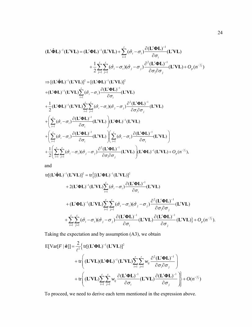
To proceed, we need to derive each term mentioned in the expression above.

25

1 2

1 1

1 1

1 1 1

1 2

( ) [( ) ( )] ( ) [( ) ( )]( ) [( ) ( )] [ ( ) ( )][ ( ) ( )] 2( ) ( ) ( ) ( )( ) ( ) 2( ) ( ) ( )

i

O n

−

− −

− −

− − −

− −

′ ′

′ ′ ′ ′ ′ ′= + +

′ ′ ′ ′= + +

′ ′ ′ ′ ′ ′= + +

′ ′= + +

L ΦL L VLL ΦL L ΦL L ΛL L ΦL L ΦL L ΛLΙ L ΦL L ΛL Ι L ΦL L ΛLΙ L ΦL L ΛL L ΦL L ΛL L ΦL L ΛLΙ L ΦL L ΛL (3.2)

1 1

1

( ) ( )( ) ( ) [( ) ( )]( ) [( ) ( ) ( ) 2( ) ( )( ) ( )ii − −

−

′ ′ ′ ′ ′ ′ ′ ′= + +

′ ′ ′ ′ ′= + +

L VL L ΦL L VL L ΦL L ΛL L ΦL L ΦL L ΛLL ΦL L ΛL L ΛL L ΦL L ΛL

]

2 11

1 1

( )So, tr ( )( ) ( )r r

iji j i j

wσ σ

−−

= =

⎡ ⎤′∂′ ′ ′⎢ ⎥∂ ∂⎢ ⎥⎣ ⎦

∑∑ L ΦLL VL L ΦL L VL

2 1 2 1

1 1 1 1

( ) ( ) tr ( ) 2 tr ( )r r r r

ij iji j i ji j i j

w wσ σ σ σ

− −

= = = =

⎡ ⎤ ⎡′ ′∂ ∂′ ′= +⎢ ⎥ ⎢∂ ∂ ∂ ∂⎢ ⎥ ⎢⎣ ⎦ ⎣

∑∑ ∑∑L ΦL L ΦLL ΦL L ΛL⎤⎥⎥⎦

2 11

1 1

( ) tr ( )( ) ( )r r

iji j i j

wσ σ

−−

= =

⎡ ⎤′∂ ′ ′ ′+ ⎢ ⎥∂ ∂⎢ ⎥⎣ ⎦

∑∑ L ΦL L ΛL L ΦL L ΛL

2 12

1 1

( ) tr ( ) ( )r r

iji j i j

w Oσ σ

−−

= =

⎡ ⎤′∂ ′= +⎢ ⎥∂ ∂⎢ ⎥⎣ ⎦

∑∑ L ΦL L ΦL n

22

1 1 1 1

2 tr( ) tr ( ), (3.3)r r r r


w w O nσ σ

−

= = = =

⎛ ⎞∂= − +⎜ ⎟⎜ ⎟∂ ∂⎝ ⎠∑∑ ∑∑ ΦΘΦΡ ΦΘΦΡ Φ Θ

where the last expression above is obtained by utilizing (3.1).

Alternatively, we can utilize lemma 2.4.8, to rewrite expression (3.3) as

22

1 1

1 2 2 tr[ ( ) ] ( )2

r r

ij i j ij iji i

A w O −

= =

− − +∑∑ ΘΦ Ρ ΦΡ Q R Φ n+ .

1 1( ) ( )( ) ( ) ( )i j

iiiσ σ

− −′ ′∂ ∂′ ′∂ ∂


1 1

1 1

( ) ( )( ) [( ) ( )]

( ) ( )( ) [( ) ( )]

i

j

σ

σ

− −

− −

∂′ ′ ′ ′ ′= + ×∂

∂′ ′ ′ ′ ′+∂

ΦL ΦL L L L ΦL L ΦL L ΛL

ΦL ΦL L L L ΦL L ΦL L ΛL

1 1 ( ) ( )( ) ( )i jσ σ

− −∂ ∂′ ′ ′ ′=∂ ∂Φ ΦL ΦL L L L ΦL L L

26

1 1 1

1 1 1

( ) ( )( ) ( )( ) ( )

( ) ( )( ) ( )( ) ( ) ( )

i j

i j

O n

σ σ

σ σ

− − −

− − −

∂ ∂′ ′ ′ ′ ′ ′+∂ ∂

∂ ∂′ ′ ′ ′ ′ ′+ +∂ ∂

Φ ΦL ΦL L L L ΦL L L L ΦL L ΛL

Φ ΦL ΦL L L L ΦL L ΛL L ΦL L L 2−

1 1

1 1

2

1 1

And hence,

( ) ( ) tr ( ) ( )

tr[ tr( ) ( )

r r

iji j i j

r r

ij i ji j

w

w O

σ σ

− −

= =

−

= =

⎛ ⎞′ ′∂ ∂′ ′⎜ ⎟⎜ ⎟∂ ∂⎝ ⎠

= +

∑∑

∑∑


ΘΦΡΦΘΦΡ Φ n

22 ( ) (3.4)A O n−= +

From we obtain ( ), ( ), and ( ),i ii iii

32

221 1

ˆ[Var[ | ]]2 1 2tr( ) 3 2 tr[ ( ) ] ( ) (3.5)

2

r r

ij i j ij iji i

F

A w O n−

= =

Ε =

⎧ ⎫+ + − − + +⎨ ⎬⎩ ⎭

∑∑

σ

ΘΛ ΘΦ ΡΦΡ Q R Φ

( ) ( ) 1

2

221 12

1 ˆˆB. Var[E[ | ]] Var[tr[( ) ( )]

1 ˆ ˆ tr[( ) ( )] tr[( ) ( )]

F −

− −

′ ′=

′ ′ ′ ′= Ε − Ε

σ L ΦL L VL


For the first term above, and by 1ˆusing a Taylor series expansion for ( ) about ,−′L ΦL σ

( )121 1

1

( )ˆ ˆtr[( ) ( ) tr ( ) ( ) ( ) ( )r

i ii i

σ σσ

−− −

=

⎡ ′∂′ ′ ′ ′ ′= + −⎢ ∂⎣∑ L ΦLL ΦL L VL L ΦL L VL L VL

32

2 1

1 1

1 ( )ˆ ˆ ( )( ) ( ) ( ) (same terms)2

r r

i i j j pi i i j

O nσ σ σ σσ σ

−−

= =

⎤′∂ ′+ − − + ×⎥∂ ∂ ⎥⎦

∑∑ L ΦL L VL

( )121 1

1

( )ˆtr[( ) ( )] 2tr[( ) ( )] ( )tr ( )r

i ii i

σ σσ

−− −

=

⎡ ⎤′∂′ ′ ′ ′ ′= + − ⎢ ⎥∂⎣ ⎦∑ L ΦLL ΦL L VL L ΦL L VL L VL

2 11

1 1

( )ˆ ˆ tr[( ) ( )] ( )( )tr ( )r r

i i j ji j i j

σ σ σ σσ σ

−−

= =

⎡ ⎤′∂′ ′ ′+ − − ⎢ ⎥∂ ∂⎢ ⎥⎣ ⎦

∑∑ L ΦLL ΦL L VL L VL

27

32

1 1

1 1

( ) ( )ˆ ˆ ( )( )tr ( ) tr ( ) ( )r r

i i j j pi j i j

O nσ σ σ σσ σ

− −−

= =

⎡ ⎤⎡ ⎤′ ′∂ ∂′ ′+ − − +⎢ ⎥⎢ ⎥∂ ∂⎢ ⎥⎣ ⎦ ⎣ ⎦∑∑ L ΦL L ΦLL VL L VL

Taking the expectation, and by assumption (A4), we have

( ) ( )2 21 1

2 11

1 1

1

1 1

tr[( ) ( )] tr[( ) ( )]

( ) tr ( ) tr[( ) ( )]

( ) tr ( ) tr

r r

iji j i j

r r

iji j i

w

w

σ σ

σ

− −

−−

= =

−

= =

′ ′ ′ ′Ε =

⎡ ⎤′∂ ′ ′ ′+ ⎢ ⎥∂ ∂⎢ ⎥⎣ ⎦

⎡ ⎤′∂ ′+ ⎢ ⎥∂⎣ ⎦

∑∑

∑∑



L ΦL L VL 32

1( ) ( ) (j

O nσ

−−⎡ ⎤′∂ ′ +⎢ ⎥

∂⎢ ⎥⎣ ⎦

L ΦL L VL )

To proceed, we need to derive each term mentioned in the expression above.

( )

1 1

1

21 2 2

( ) ( ) ( ) ( ) ( )tr[( ) ( )] tr( )

tr[( ) ( )] 2 tr( ) ( ) (3.6)

i

O n

− −

−

− −

′ ′ ′ ′= +

′ ′⇒ = +

′ ′⇒ = + +

L ΦL L VL Ι L ΦL L ΛLL ΦL L VL ΘΛ

L ΦL L VL ΘΛ

1 1 1

1 1 1

1

( ) ( ) ( )( ) ( ) ( ) ( )

( ) ( ) ( ) ( )

( )So, tr ( ) tr( ) tr( )

i i i

i i

i ii

iiσ σ σ

σ σ

σ

− − −

− − −

−

′ ′ ′∂ ∂ ∂′ ′ ′= +∂ ∂ ∂

∂ ∂′ ′ ′ ′ ′ ′= − −∂ ∂

⎡ ⎤′∂ ′ = − −⎢ ⎥∂⎣ ⎦

L ΦL L ΦL L ΦLL VL L ΦL L ΛL

Φ ΦL ΦL L L L ΦL L L L ΦL L ΛL

L ΦL L VL ΘΦΡ Φ ΘΦΡΦΘΛ , (3.7)

2 1 2 1 2 1( ) ( ) ( )( ) ( ) ( ) ( )i j i j i j

iiiσ σ σ σ σ σ

− − −′ ′ ′∂ ∂ ∂′ ′ ′= +∂ ∂ ∂ ∂ ∂ ∂L ΦL L ΦL L ΦLL VL L ΦL L ΛL ,

2 1

2 1 2 1

( )and tr ( )

( ) ( ) tr ( ) tr ( )

i j

i j i j

σ σ

σ σ σ σ

−

− −

⎡ ⎤′∂ ′⎢ ⎥∂ ∂⎢ ⎥⎣ ⎦

⎡ ⎤ ⎡′ ′∂ ∂′ ′= +⎤

⎢ ⎥ ⎢∂ ∂ ∂ ∂

⎥⎢ ⎥ ⎢ ⎥⎣ ⎦ ⎣

L ΦL L VL

L ΦL L ΦLL ΦL L ΛL⎦

2

2tr( ) tr 2tr( )i j i ji jσ σ

⎛ ⎞∂= − +⎜ ⎟⎜ ⎟∂ ∂⎝ ⎠

ΦΘΦΡ ΦΘΦΡ Φ Θ ΘΦΡ ΦΘΦΡ ΦΘΛ

2

tr (from expression 3.1). (3.8)i jσ σ

⎛ ⎞∂− ⎜ ⎟⎜ ⎟∂ ∂⎝ ⎠

ΦΘ ΘΛ

28

( )21 2

From ( ), ( ), and ( ),

ˆtr[( ) ( ) 2 tr( )

i ii iii−′ ′Ε =L ΦL L VL ΘΛ+

2

1 1 [ tr( )] tr 2tr( )

r r

ij i ji j i j

wσ σ= =

⎧ ⎛ ⎞⎪⎜ ⎟⎨ ⎜ ⎟⎪ ⎝ ⎠⎩

∂+ + − +∂ ∂∑∑ ΦΘΛ Θ ΘΦΡ ΦΘΦΡ Φ

3

2

2

1 1

( )

2tr( ) tr

[tr( ) tr( )][tr( ) tr( )]

i ji j

r r

ij i i j ji j

O nw

σ σ

−

= =

⎫⎛ ⎞⎪⎜ ⎟⎬⎜ ⎟⎪⎝ ⎠⎭

∂+ −∂ ∂

+ + +∑∑

ΦΘΦΡ ΦΘΦΡ ΦΘΛ Θ ΘΛ

ΘΦΡ Φ ΘΦΡΦΘΛ ΘΦΡ Φ ΘΦΡ ΦΘΛ +

22

1 1

2

2 2

2 tr( ) 2 tr( ) tr

2 tr( ) tr 2tr( )tr( )

tr( )tr 2tr( )tr( ) tr( )tr

r r

ij i ji j i j

i j i ji j

i ji j

wσ σ

σ σ

σ σ σ

= =

⎧ ⎛ ⎞∂⎪= + + − ⎜ ⎟⎨ ⎜ ⎟∂ ∂⎪ ⎝ ⎠⎩⎛ ⎞∂

+ − +⎜ ⎟⎜ ⎟∂ ∂⎝ ⎠⎛ ⎞∂ ∂

− + −⎜ ⎟⎜ ⎟∂ ∂ ∂⎝ ⎠

∑∑ ΦΘΛ ΘΦΡ ΦΘΦΡ Φ Θ

ΦΘΦΡ ΦΘΦΡ ΦΘΛ Θ θΛ ΘΛ ΘΦΡ ΦΘΦΡ Φ

Φ ΦΘΛ Θ ΘΛ ΘΦΡ ΦΘΦΡ ΦΘΛ ΘΛ Θ

3

2

tr( )tr( ) 2tr( )tr( ) tr( )tr( )

( )

i j

i j i j i j

O n

σ

−

⎛ ⎞⎜ ⎟⎜ ⎟∂⎝ ⎠

+ + +

+

ΘΛ

ΘΦΡ Φ ΘΦΡ Φ ΘΦΡ Φ ΘΦΡ ΦΘΛ ΘΦΡ ΦΘΛ ΘΦΡ ΦΘΛ

32

32

22

1 1

1 1

22

2 11 1

2 tr( ) 2 tr( ) tr

tr( )tr( ) ( )

2 tr( ) 2 tr ( ),

r r

ij i ji j i j

r r

ij i ji j

r r

iji j i j

w

w O n

A A w O n

σ σ

σ σ

= =

−

= =

−

= =

⎧ ⎫⎛ ⎞∂⎪ ⎪= + + − ⎜ ⎟⎨ ⎬⎜ ⎟∂ ∂⎪ ⎪⎝ ⎠⎩ ⎭

+ +

⎛ ⎞∂= + + + − +⎜ ⎟⎜ ⎟∂ ∂⎝ ⎠

∑∑

∑∑

∑∑

ΦΘΛ ΘΦΡ ΦΘΦΡ Φ Θ

ΘΦΡ Φ ΘΦΡ Φ

ΦΘΛ Θ (3.9)

11 1

where tr( )tr( ).r r

ij i ji j

A w= =

=∑∑ ΘΦΡΦ ΘΦΡ Φ

Also, from expression 3.2,

( )21 2 2

2 3ˆtr[( ) ( )] 2 ( +2 ) ( ) (3.10)A A O n− −⎡ ⎤′ ′Ε = + +⎣ ⎦L ΦL L VL

From expressions (3.9) and (3.10), we obtain

29

32

22 2

2 1 2 321 1

ˆVar[E[ | ]]

1 2 tr( ) 2 tr 2 ( +2 ) ( )r r

iji j i j

F

A A w A A O nσ σ

−

= =

⎧ ⎫⎛ ⎞∂⎪ ⎪= + + + − − − +⎜ ⎟⎨ ⎬⎜ ⎟∂ ∂⎪ ⎪⎝ ⎠⎩ ⎭∑∑

σ

ΦΘΛ Θ

32

2

1 321 1

1 2 tr( ) tr 4 ) ( )r r

iji j i j

A w A O nσ σ

−

= =

⎧ ⎫⎛ ⎞∂⎪ ⎪= + − − +⎜ ⎟⎨ ⎬⎜ ⎟∂ ∂⎪ ⎪⎝ ⎠⎩ ⎭∑∑ ΦΘΛ Θ

From parts (A) and (B), we are able to find an expression for . Var[ ]F

32

2

221 1

2

1 321 1

2Var[ ] 2tr( ) 3 tr

1 2 tr( ) tr 4 ( )

r r

iji j i j

r r

iji j i j

F A w

A w A O n

σ σ

σ σ

= =

−

= =

⎧ ⎫⎛ ⎞∂⎪ ⎪= + + − ⎜ ⎟⎨ ⎬⎜ ⎟∂ ∂⎪ ⎪⎝ ⎠⎩ ⎭⎧ ⎫⎛ ⎞∂⎪ ⎪+ + − − +⎜ ⎟⎨ ⎬⎜ ⎟∂ ∂⎪ ⎪⎝ ⎠⎩ ⎭

∑∑

∑∑

ΦΘΛ Θ

ΦΘΛ Θ

32

22 1

31 1

32 2 1 11 2 1 tr( ) tr2 2

r r

iji j i j

A A A wσ σ

−

= =

⎧ ⎫⎛ ⎞∂⎪ ⎪⎛ ⎞ ⎛ ⎞= + + − + + − + +⎜ ⎟⎨ ⎬⎜ ⎟ ⎜ ⎟ ⎜ ⎟∂ ∂⎝ ⎠ ⎝ ⎠⎪ ⎪⎝ ⎠⎩ ⎭∑∑ ΦΘΛ Θ ( )O n

32

32

2

1 2 31 1

2

1 2 31 1

2 11 6 4 2( 2)tr( ) ( 2) tr ( )2

2 11 6 4 ( 2) 2tr( ) tr (2

r r

iji j i j

r r

iji j i j

A A A w O n

A A A w O n

σ σ

σ σ

−

= =

−

= =

⎧ ⎫⎡ ⎤⎛ ⎞∂⎪ ⎪= + + − + + − + +⎢ ⎥⎜ ⎟⎨ ⎬⎜ ⎟∂ ∂⎢ ⎥⎪ ⎪⎝ ⎠⎣ ⎦⎩ ⎭⎧ ⎫⎡ ⎤⎧ ⎫⎛ ⎞∂⎪ ⎪ ⎪⎢ ⎥= + + − + + − +⎜ ⎟⎨ ⎨ ⎬⎜ ⎟∂ ∂⎢ ⎥⎪ ⎪⎪ ⎪⎝ ⎠⎩ ⎭⎣ ⎦⎩ ⎭

=

∑∑

∑∑

ΦΘΛ Θ

ΦΘΛ Θ )⎪⎬

32

1 2 31 1

2 11 6 4 ( 2) 4tr( ) tr( ) ( ),2

r r

ij iji j

A A A w O n−

= =

⎧ ⎫⎡ ⎤⎧ ⎫⎪ ⎪+ + − + + − +⎢ ⎥⎨ ⎨ ⎬ ⎬⎢ ⎥⎩ ⎭⎪ ⎪⎣ ⎦⎩ ⎭

∑∑ΘΛ ΘΦR Φ

52

52

2

1 1

1 1

31 1

by noticing that

tr

2tr( ) tr( ) ( ) (lemmas 2.4.8 and 2.4.10),

1and tr( ) tr( ) ( ).4

r r

iji j i j

r r

ij iji j

r r

ij iji j

w

w O n

A w O n

σ σ= =

−

= =

−

= =

⎛ ⎞∂− =⎜ ⎟⎜ ⎟∂ ∂⎝ ⎠

− +

= − +

∑∑

∑∑

∑∑

ΦΘ

ΘΛ ΘΦR Φ

ΘΛ ΘΦR Φ

Proposition 3.1.1.2.1 32

12Var[ ] (1 ) ( ),F B O n−= + +

30

[ ]1 1 2 31where 6 +8 2

B A A A= +

3.1.2 Constructing a Wald-Type Pivot Through AΦ

The Wald type pivot is 1A

1 ˆ ˆ( ) ( ) (F −′ ′ ′ ˆ )= −β β L L Φ L L β β−

F

2−

. Similar to section

3.1.1, we derive expressions for approximately E[ ] and Var[ ]F

3.1.2.1 Deriving an Approximate Expression for E[F]

First, we derive a useful lemma that will be needed in this section and chapter 4.

Lemma 3.1.2.1.1 1 1For a matrix ( ), ( ) ( )p pO n O n− −+ = − +B = Ι B Ι B

Proof 1 1( ) ( ) (Schott, 2005, theorem 1.7)− −+ = − +Ι B Ι Ι B B

1 1

1 1 1

1 1

( ) , applying the theorem again for ( )

Notice that since , then ( ) ( ) , and hence ( ) (1).

Therefore, ( ) ( ) (

p p

pO

O n

− −

− − −

− −

⎡ ⎤= − − + +⎣ ⎦

→ + → + = + =

+ = − + + = − +

Ι Ι Ι B B B Ι B

B 0 Ι B Ι 0 Ι Ι B

Ι B Ι B Ι B BB Ι B 2 ). −

( )1A

1 ˆˆˆ[ | ] tr ( ) Var[ ( )]F −′ ′Ε = −σ L Φ L L β β , by assumption (A4).

( )( )

1A

1A

A1 1

1A

ˆˆ[ ] E tr[( ) ( )] , where Var( )

ˆ tr E[( ) ( )]

1ˆ ˆ ˆˆ ˆ ˆ ˆ ˆ ˆ ˆ ˆˆSince where 2 ( ) ,4

ˆ ˆthen ( ) ( ) (

r r

ij ij i j iji j

F

w

−

−

∗ ∗

= =

−

′ ′⇒ Ε = = = +

′ ′=

⎧ ⎫= + = − −⎨ ⎬

⎩ ⎭

′ ′ ′=

∑∑

L Φ L L VL V β Φ Λ

L Φ L L VL

Φ Φ A A Φ Q Ρ ΦΡ R Φ

L Φ L L VL L

1

11

11 1

ˆ) ( ) ( )

ˆˆ ˆ ( ) ( ) ( ) ( )

ˆˆ ˆ ( ) ( ) ( ) ( ).

−∗

−− ∗

−− ∗ −

⎡ ⎤′ ′+⎣ ⎦

⎡ ⎤′ ′ ′ ′= +⎣ ⎦

⎡ ⎤′ ′ ′ ′= +⎣ ⎦

ΦL L A L L VL

L ΦL Ι L ΦL L A L L VL

Ι L ΦL L A L L ΦL L VL

1 1ˆˆSince ( ) ( ) ( ), then by employing the lemma 3.1.2.1.1, pO n− ∗ −′ ′ =L ΦL L A L

31

1 1 2A

ˆˆ ˆ ˆ( ) ( ) ( ) ( ) ( ) ( ) (pO n− − ∗ −⎡ ⎤′ ′ ′ ′ ′ ′= − +⎣ ⎦L Φ L L VL Ι L ΦL L A L L ΦL L VL1 )−

1)

1 1 1 2ˆˆ ˆ ˆ( ) ( ) ( ) ( )( ) ( ) ( ) (3.1pO n− − ∗ − −′ ′ ′ ′ ′ ′= − +L ΦL L VL L ΦL L A L L ΦL L VL

( ) 321

2 3

1 1

1 1

ˆNotice that E tr[( ) ( )] A 2A ( ), (3.12)

(proposition 3.1.1.1.1) ˆˆ ând ( ) ( )( ) ( )ˆˆ ˆ ( ) ( )( )

O n−−

− ∗ −

− ∗ −

′ ′ = + + +

′ ′ ′ ′

′ ′ ′=

L ΦL L VL

L ΦL L A L L ΦL L VL

L ΦL L A L L ΦL 1 1ˆˆ ˆ( ) ( ) ( )( ) ( )− ∗ −′ ′ ′ ′ ′+L ΦL L ΦL L A L L ΦL L ΛL

1 1 .ˆˆ ˆ( ) ( )( ) ( ) (pO n− ∗ − −′ ′ ′ ′= +L ΦL L A L L ΦL L ΦL 2 )

2

1

1 1 ( )

Ûsing a Taylor series expansion for ( ) about , we haveˆˆ ˆ( ) ( )( ) ( ) pO n−

−

− ∗ −

′

′ ′ ′ ′ +

L ΦL σ

L ΦL L A L L ΦL L ΦL

1 2 11

1 1 1

1 2 11 2

1 1 1

( ) 1 ( ) ˆˆ ˆ ˆ( ) ( ) ( )( ) ( )2

( ) 1 ( )ˆ ˆ ˆ( ) ( ) ( )( ) ( ) (2

r r r

i i i i j ji i ji i j

r r r

i i i i j j pi i ji i j

O n

σ σ σ σ σ σσ σ σ

σ σ σ σ σ σσ σ σ

− −− ∗

= = =

− −− −

= = =

⎡ ⎤′ ′∂ ∂′ ′= + − + − −⎢ ⎥∂ ∂ ∂⎢ ⎥⎣ ⎦

⎡ ⎤′ ′∂ ∂′ ′× + − + − − +⎢ ⎥∂ ∂ ∂⎢ ⎥⎣ ⎦

∑ ∑∑

∑ ∑∑

L ΦL L ΦLL ΦL L

L ΦL L ΦLL ΦL L ΦL )

A L

321 ˆ ( ) ( ) ( ) (3.13)pO n−− ∗′ ′= +L ΦL L A L

32

2 3

From expressions (3.12 and 3.13), we obtainˆ[ ] 2 E tr( ) ( ) (3.14)F A A O n−∗⎡ ⎤Ε = + + − +⎣ ⎦ΘA

Lemma 52Ê[ ] ( )O n−∗ ∗= +A A

Proof Direct from Lemmas 2.4.10 and 2.4.11

Applying the lemma above on expression (3.14), we have

Proposition 3.1.2.1.2 322[ ] 1 ( )AF O n−

Ε = + +

3.1.2.2 Deriving an Approximate Expression for Var[F]

ˆ ˆ Var[ ] E[Var[ | ]] Var[E[ | ]]F F F= +σ σ

32

1A2

1 ˆ ˆˆˆ Â. Var[ | ]] Var[( ) ( ) ( ) | ]F −′ ′ ′= − −σ β β L L Φ L L β β σ

The expression above is a quadratic form and hence by assumption (A4), 1 2

A2

2 ˆˆ Var[ | ]] tr[( ) ( )] ] (Schott, 2005, theorem 10.22).F −′ ′=σ L Φ L L VL

( )

1 1 1 1A

21 2 1A

Recall that from expression (3.11), we hadˆˆ ˆ ˆ ˆ( ) ( ) ( ) ( ) ) ( )( ) ( ) ( ).

ˆ ând hence, tr [( ) ( )] tr ( ) ( )

2

pO n− − − ∗ −

− −

′ ′ ′ ′ ′ ′ ′ ′= − +

⎡ ⎤′ ′ ′ ′= ⎣ ⎦

−

L Φ L L VL L ΦL L VL L ΦL L A L L ΦL L VL

L Φ L L VL L ΦL L VL

1 1 1ˆˆ ˆ ˆtr ( ) ( )( ) ( )( ) ( ) (pO n− − ∗ −⎡ ⎤′ ′ ′ ′ ′ ′ +⎣ ⎦L ΦL L VL L ΦL L A L L ΦL L VL

2−

2 )−

2−+

( ) ( )

( ) ( )

1 1

1 1 1

1 1 1 1

ˆ ˆtr ( ) ( ) ( ) ( ) ( ) ( )

ˆˆ ˆ ˆ2tr ( ) ( ) ( ) ( ) ( )( ) ( ) ( ) ( )

ˆ ˆ ˆ ˆtr ( ) ( )( ) ( ) 2tr ( ) ( )( ) ( )

pO n

− −

− − ∗ −

− − − −

⎡ ⎤′ ′ ′ ′ ′ ′= + +⎣ ⎦⎡ ⎤′ ′ ′ ′ ′ ′ ′ ′− + +⎣ ⎦⎡ ⎤ ⎡′ ′ ′ ′ ′ ′ ′ ′= +⎣ ⎦

L ΦL L ΦL L ΛL L ΦL L ΦL L ΛL

L ΦL L ΦL L ΛL L ΦL L A L L ΦL L ΦL L ΛL

L ΦL L ΦL L ΦL L ΦL L ΦL L ΦL L ΦL L ΛL

1 1 1 2ˆˆ ˆ ˆ 2tr ( ) ( )( ) ( )( ) ( ) ( ).pO n− − ∗ − −

⎤⎣ ⎦⎡ ⎤′ ′ ′ ′ ′ ′− +⎣ ⎦L ΦL L ΦL L ΦL L A L L ΦL L ΦL

( )1 2

1 1 1

1

1 2A

( ) 1 ( )ˆ ˆ ˆtr ( ) ( ) ( )( ) ( ) 2

( )ˆ( )

Ûsing a Taylor series expansion for ( ) about , we haveˆtr [( ) ( )]

r r r


i i

σ σ σ σ σ σσ σ

σ σ

− −

= = =

−

−

−

′ ′∂ ∂′ ′+ − + − −∂ ∂

′∂× + −

′

′ ′ =

⎧⎡ ⎤⎪⎨⎢ ⎥⎪⎣ ⎦⎩

∑ ∑∑L ΦL L ΦLΙ L ΦL L ΦL

L ΦLΙ

L ΦL σ

L Φ L L VL

1

σ∂

1 2

1 1 1

1 2

1 1 1

1 ( )ˆ ˆ( ) ( )( ) ( )2

( ) 1 ( )ˆ ˆ ˆ2tr ( ) ( ) ( )( ) ( )2

r r r

i i j ji i ji i j

r r r


σ σ σ σσ σ


−

= = =

− −

= = =

′∂′ ′+ − −∂ ∂

′ ′∂ ∂′ ′+ + − + − −∂ ∂

⎫⎡ ⎤⎪⎬⎢ ⎥⎪⎣ ⎦⎭

⎧⎡ ⎤⎪⎨⎢ ⎥⎪⎣ ⎦⎩

∑ ∑∑

∑ ∑∑

L ΦLL ΦL L ΦL

L ΦL L ΦLΙ L ΦL L ΦL

1

1

σ

σ

∂

∂

1 21

1 1 1

( ) 1 ( )ˆ ˆ ˆ( ) ( ) ( ) ( ) ( )( ) ( )2

r r r



− −−

= = =

′ ′∂ ∂′ ′ ′ ′× + − + − −∂ ∂

⎫⎡ ⎤1

σ∂⎪⎬⎢ ⎥⎪⎣ ⎦⎭

∑ ∑∑L ΦL L ΦLL ΦL L ΛL L ΛL L ΛL

1 2

1 1 1

1 2

21 1 1

( ) 1 ( )ˆ ˆ ˆ2tr ( ) ( ) ( )( ) ( )2

( ) 1 ( )ˆ ˆ ˆ( ) ( ) ( )( ) (2

r r r


r r r

i i i i j ji i ji i



− −

= = =

− −

= = =

′ ′∂ ∂′ ′− + − + − −∂ ∂

⎧⎡ ⎤⎪⎨⎢ ⎥⎪⎣ ⎦⎩

⎡ ⎤′ ′∂ ∂′ ′× + − + − −⎢ ⎥∂ ∂⎢ ⎥⎣ ⎦

∑ ∑∑

∑ ∑∑



1

1

)j

σ

σ

∂

∂

33

11

1

( )ˆ ˆˆ( ) ( ) ( ) ( )r

i ii i

σ σσ

−− ∗ ∗

=

×⎡ ′∂′ ′ ′+ −⎢ ∂⎣

∑ L ΦLL ΦL L A L L A L

2 12

1 1

1 ( ) ˆˆ ˆ ( )( ) ( ) ( )2

r r

i i j j pi j i j

O nσ σ σ σσ σ

−∗ −

= =

⎫⎤′∂ ⎪′+ − − +⎥⎬∂ ∂ ⎥⎪⎦⎭

∑∑ L ΦL L A L

1 2

1 1 1

1 1

1 1

1

tr

tr

( ) ( )ˆ ˆ ˆ2 ( ) ( ) ( )( ) ( )

( ) ( )ˆ ˆ ( )( ) ( ) ( )

2tr ( ) ( )

r r r

i i i i j ji i ji i

r r

i i j ji j i j


σ σ σ σσ σ

− −

= = =

− −

= =

−

=⎡ ⎤′ ′∂ ∂′ ′+ − + − −⎢ ⎥

∂ ∂⎢ ⎥⎣ ⎦⎡ ⎤′ ′∂ ∂′ ′+ − −⎢ ⎥

∂ ∂⎢ ⎥⎣ ⎦

′ ′⎡ ⎤+ ⎣

∑ ∑∑

∑∑


L ΦL L ΦLL ΦL L ΦL

L ΦL L ΛL

1

jσ∂

321 ˆ2tr ( ) ( ) ( ).pO n−− ∗⎡ ⎤′ ′− +⎦ ⎣ ⎦L ΦL L A L

32

2 1

21 1

1 1

1 1

By taking the expectation and assumption (A3),

2 ( )ˆE[Var[ | ]] tr

( ) ( ) tr 2tr[ ] 2tr[ ] (

r r

iji j i j

r r

iji j i j

F w

w O

σ σ

σ σ

−

= =

− −−∗

= =

⎧ ⎡ ⎤′∂⎪ ′= + ⎢ ⎥⎨∂ ∂⎢ ⎥⎪ ⎣ ⎦⎩

⎫⎡ ⎤′ ′∂ ∂ ⎪′ ′+ +⎢ ⎥ ⎬∂ ∂⎢ ⎥ ⎪⎣ ⎦ ⎭

∑∑

∑∑

L ΦLσ L ΦL

L ΦL L ΦLL ΦL L ΦL ΘΛ ΘA ).n− +

1 1

21 1

2 1 2

21 1 1 1

2

( ) ( )Notice that tr ,

( ) ( )and from (3.1), tr 2 tr .

Hence,

2ˆE[Var[ | ]] 3

r r

iji j i j

r r r r

ij iji j i ji j i j

w A

w A w

F

σ σ

σ σ σ σ

− −

= =

−

= = = =

⎡ ⎤′ ′∂ ∂′ ′ =⎢ ⎥∂ ∂⎢ ⎥⎣ ⎦⎡ ⎤ ⎡′ ′∂ ∂′ = −⎢ ⎥ ⎢

∂ ∂ ∂ ∂⎢ ⎥ ⎢⎣ ⎦ ⎣

= +

∑∑

∑∑ ∑∑

L ΦL L ΦLL ΦL L ΦL

L ΦL L ΦLL ΦL Θ

σ

⎤⎥⎥⎦

32

2

21 1

( )2tr[ ] 2tr[ ] tr ( ).r r

iji j i j

A wσ σ

−∗

= =

⎧ ⎫⎡ ⎤′∂⎪ ⎪+ − − +⎢ ⎥⎨ ⎬∂ ∂⎢ ⎥⎪ ⎪⎣ ⎦⎩ ⎭∑∑ L ΦLΘΛ ΘA Θ O n

32

2

1 1

2

1 1

In addition, by lemmas 2.4.8 and 2.4.10, we have

( ) 2tr[ ] 2tr[ ] tr

( ) 2tr[ ] 2tr[ ] tr ( )

r r

iji j i j

r r

iji j i j

w

w O

σ σ

σ σ

∗

= =

−∗

= =

⎡ ⎤′∂− − ⎢ ⎥

∂ ∂⎢ ⎥⎣ ⎦⎡ ⎤′∂

= − − +⎢ ⎥∂ ∂⎢ ⎥⎣ ⎦

∑∑

∑∑

L ΦLΘΛ ΘA Θ

L ΦLΘΛ ΘA Θ n

1 1 1 1

1 2 tr ( ) 4 tr ( )4

r r r r

ij ij i j ij ij i j iji j i j

w w= = = =

⎡ ⎤⎡ ⎤= − − − −⎣ ⎦ ⎢ ⎥⎣ ⎦∑∑ ∑∑ΘΦ Q Ρ ΦΡ Φ ΘΦ Q Ρ ΦΡ R Φ

34

3 3 32 2 2

1 1

12 tr ( ) ( ) 0 ( ) ( ) (3.15)2

r r

ij i j ij iji j

w O n O n O n− − −

= =

⎡ ⎤− − + + = + =⎢ ⎥⎣ ⎦∑∑ ΘΦ Ρ ΦΡ Q R Φ

32

22

2ˆ E[Var[ | ]] 3 ( ) (3.16)F A O n−⇒ = + +σ

( ) ( ) 1

A2

221 1A A2

1 ˆˆB. Var[E[ | ]] Var[tr[( ) ( )], by assumption (A4)

1 ˆ ˆ tr[( ) ( )] tr[( ) ( )] ,

F −

− −

′ ′=

′ ′ ′ ′= Ε − Ε

σ L Φ L L VL

L Φ L L VL L Φ L L VL

1)

( )

21A

21 1 2

ˆ( ) tr[( ) ( )

ˆˆ ˆ ˆ tr ( ) ( ) ( )( )( ) ( ) ( ) (from 3.1p

i

O n

−

− ∗ − −

′ ′

⎡ ⎤′ ′ ′ ′ ′ ′= − +⎣ ⎦

L Φ L L VL

L ΦL L VL L ΦL L A L L ΦL L VL

21 1

2

21 1

ˆˆ ˆ ˆ ˆ tr ( ) ( ) 2tr ( ) ( ) tr ( )( )( ) ( )

( )

ˆˆ ˆ ˆ ˆ tr ( ) ( ) 2tr ( ) ( ) tr ( )( )( ) ( )

pO n

O

− − ∗

−

− − ∗

1

1

−

−

⎡ ⎤⎡ ⎤ ⎡ ⎤′ ′ ′ ′ ′ ′ ′ ′= −⎣ ⎦ ⎣ ⎦ ⎣ ⎦+

⎡ ⎤⎡ ⎤ ⎡ ⎤′ ′ ′ ′ ′ ′ ′ ′= −⎣ ⎦ ⎣ ⎦ ⎣ ⎦+

L ΦL L VL L ΦL L VL L ΦL L A L L ΦL L VL

L ΦL L VL L ΦL L ΦL L ΦL L A L L ΦL L ΦL2( ) (recall that ).p n− = +V Φ Λ

( )3

2

21

22

2 11 1

1

ˆFrom expression (3.9), E tr[( ) ( )]

2 tr[ ] 2 tr ( ).

ˆ( ) Using a Taylor series expansion for ( ) about , we have

tr

r r

iji j i j

A A w O n

ii

σ σ

−

−

= =

−

′ ′

⎡ ⎤∂= + + + − +⎢ ⎥

∂ ∂⎢ ⎥⎣ ⎦′

∑∑

L ΦL L VL

ΦΘΛ Θ

L ΦL σ1 1 1ˆˆ ˆ ˆ( ) ( ) tr ( ) ( )( ) ( )− − ∗ −⎡ ⎤⎡ ⎤′ ′ ′ ′ ′ ′⎣ ⎦ ⎣ ⎦ =L ΦL L ΦL L ΦL L A L L ΦL L ΦL

1 2

1 1 1

1 2

1 1 1

( ) 1 ( )ˆ ˆ ˆtr ( ) ( ) ( )( ) ( )2

( ) 1 ( )ˆ ˆ ˆtr ( ) ( ) ( )( ) ( )2

r r r


r r r




− −

= = =

− −

= = =

′ ′∂ ∂′ ′+ − + − −∂ ∂

′ ′∂ ∂′ ′× + − + − −∂ ∂

⎡ ⎤⎢ ⎥⎣ ⎦⎧⎡ ⎤⎪⎨⎢ ⎥⎪⎣ ⎦⎩

∑ ∑∑

∑ ∑∑



1

1

σ

σ

∂

∂

11

1

( )ˆ ˆˆ( ) ( ) ( ) ( )r

i ii i

σ σσ

−− ∗ ∗

=

×⎡ ′∂′ ′ ′+ −⎢ ∂⎣

∑ L ΦLL ΦL L A L L A L

52

2 1

1 1

1 ( ) ˆˆ ˆ( )( ) ( )2

( ).r r

i i j ji j i j

pO nσ σ σ σσ σ

−∗

= =

−′∂ ′+ − −∂ ∂

⎫⎤⎪+⎬⎥⎪⎦⎭

∑∑ L ΦLL A L

35

By assumption (A3), we obtain

( ) 321 1 1ˆˆ ˆ Ê tr ( ) ( ) tr ( ) ( )( ) ( ) ( ).tr[ ] O n−− − ∗ − ∗⎡ ⎤⎡ ⎤′ ′ ′ ′ ′ ′ =⎣ ⎦ ⎣ ⎦ +L ΦL L ΦL L ΦL L A L L ΦL L ΦL ΘA

From ( ) and ( ),i ii

( )21 2

A 2ˆ E tr[( ) ( )] 2 tr[ ] 2 1A A−′ ′ = + +L Φ L L VL ΘΛ +

32

32

2

1 1

2

1 1

1

tr 2 tr[ ] ( ),

and since 2tr[ ] tr 2tr[ ] ( ) (from 3.17),

then

ˆ E tr[( ) ( )

r r

iji j i j

r r

iji j i j

w O n

w O n

σ σ

σ σ

−∗

= =

−∗

= =

−

⎡ ⎤∂− − +⎢ ⎥

∂ ∂⎢ ⎥⎣ ⎦⎡ ⎤∂

− − =⎢ ⎥∂ ∂⎢ ⎥⎣ ⎦

′ ′

∑∑

∑∑

ΦΘ ΘA

ΦΘΛ Θ ΘA

L ΦL L VL( ) 32

2 22 1] 2 ( ). (3.17)A A O n−= + + +

Recall that from expression (3.14), we have

( )( )

32

32

1A 2

21 2

A 2

Ê tr ( ) ( ) E[F] ( )

Ê tr ( ) ( ) 2 ( ). (3.18)

A O n

A O n

−−

−−

⎡ ⎤′ ′ = = + +⎣ ⎦

⎡ ⎤′ ′⇒ = + +⎣ ⎦

L Φ L L VL

L Φ L L VL

From expressions (3.17 and 3.18), we obtain

32

32

2 22 1 22

12

1ˆVar[E[ | ]] 2 2 ( )

( ), (3.19)

F A A A O n

A O n

−

−

= + + − − +

= +

σ

Therefore from expressions (3.16 and 3.19),

Proposition 3.1.2.2.1 ( ) 32

2Var[ ] 1 ( ),F B O n−= + +

( )1 21where 6 .2

B A A= +

Summary

( )i When the adjusted estimate of the variance-covariance matrix is used in constructing

the Wald-type statistic,

36

( )

2 [ ] 1 ,

2and Var[ ] 1 ,

AF E

F V B

Ε ≈ = +

≈ = +

( )1 21where 6 ,2

B A A= +

1 21 1 1 1

and tr( )tr( ), tr( )r r r r

ij i j ij i ji j i j

A w A w= = = =

= =∑∑ ∑∑ΘΦΡ Φ ΘΦΡ Φ ΘΦΡ ΦΘΦΡ Φ

( )ii When the conventional estimate of the variance-covariance matrix is used,

2 31

2 E[ ] 1 A AF E +≈ = +

1 1

2 1 31

31 1

2and Var[ ] (1 ),

6 8where , 2

1and tr[ ( ) ]4

r r

ij ij i j iji j

F V B

A A AB

A w= =

≈ = +

+ +=

= − −∑∑ ΘΦ Q Ρ ΦΡ R Φ

Or alternatively,

21

1 1

2 11 2 2 3

[ ] 1

2and Var[ ] (1 ),

6where , 2 , 42

SF E

F V B

S S1 1 3B and S A A S A A

Ε ≈ = +

≈ = +

+= = + = −

3.2 Estimating the Denominator Degrees of Freedom and the Scale Factor

In order to determine and mλ such that approximately, we

match the approximated first two moments of

F( , )F F mλ∗ = ∼

F ∗ with those of distribution. F( , )m

E[F( , )] ,2

mmm

=−

2 2Var[F( , )] 2 .2 ( 4)

m mmm m

+ −⎛ ⎞= ⎜ ⎟− −⎝ ⎠

37

2

In the previous section, we found expressions for and such that

[ ] 1 ,

E VAF EΕ ≈ = +

( )2and Var[ ] 1 ,F V B≈ = +

By matching the first moments,

E[ ]2

. ( 2)

mF Em

mE m

λ

λ

∗ ≈ =−

⇒ =−

22

2

2

By matching the second moments,

2 Var[ ] 22 ( 4)

2 22 ( 2) ( 4) 2 ( 4)

m mF Vm m

m m V mVm m E m

λ

λ

∗ + −⎛ ⎞≈ = ⎜ ⎟− −⎝ ⎠

⎡ ⎤ + − + −⇔ = ⇔ =⎢ ⎥− −⎣ ⎦ −

2and hence 4 , 1

mρ+

= +− 2where .

2VE

ρ =

The scale and denominator degrees of freedom are to be estimated by substituting for

in . The quantity can be estimated by using the inverse of the expected

information matrix.

σ

σ 1 2, , and A A A3 ijw

38

4. MODIFYING THE ESTIMATES OF THE DENOMINATOR DEGREES OF FREEDOM AND THE SCALE FACTOR

As we saw in chapter three, the Wald-type statistic does not have an F

distribution usually; however, the scaled form of will have an F distribution

approximately. Indeed, there are number of special cases where the scaled form of

follows an F distribution exactly. Kenward and Roger (1997) considered two of these

special cases; the Hotelling and the conventional Anova models, and then they

modified the approximate expressions for the expectation and the variance of so the

modified expressions produce estimates of the denominator degree of freedom and the

scale that match the exact and known values for the special cases. In this chapter, we

derive Kenward and Roger (K-R) modification based on the Hotelling and the

balanced one-way Anova models.

F

F

F2T

F

2T

4.1 Balanced One-Way Anova Model

4.1.1 The Model and Assumptions

iid2

Consider the model: for 1,.., , and 1,...., ,

where is the general mean, are the treatment effects, and N(0, )

ij i ij

i i

y e i t j m

e j e

μ τ

μ τ

= + + = =

∼ σ

Suppose that we are interested in testing 0 1 tH : ..... ,τ τ ′= = ⇔ =L β 0

[ ]1 t

0 1 1 0 00 0 1 1 0

where ,

0 0 0 1 1

μ τ τ

−⎡ ⎤⎢ ⎥−⎢ ⎥′ ′= =⎢ ⎥⎢ ⎥−⎣ ⎦

L β

2 , where .n n mtσ=Σ Ι = The design matrix; is not of full column rank. We can

proceed with this parameterization, using the g-inverse, however, to simplify our

computations, we will reparameterize the model so will be a full column rank matrix

Χ

Χ

1 11

as follows with 0, and the hypothesis becomest

t ii

μ τ τ τ∗ ∗ ∗ ∗ ∗−

=

′ ⎡ ⎤= =⎣ ⎦ ∑β

39

0

0 1 0 0 00 0 1 0 0

H : , where

0 0 0 0 1

∗ ∗ ∗

⎡ ⎤⎢ ⎥⎢ ⎥′ ′= =⎢ ⎥⎢ ⎥⎣ ⎦

L β 0 L

To simplify our notation, from now on, consider , , and .∗ ∗ ∗= = =Χ Χ L L β β

4.1.2 The REML Estimates ofσ

Since the design is balanced, then the REML estimates are the same as the Anova

estimates (Searle , 1992, section 3.8), and hence .et al

2REML

( )ˆ MSE .n t

σ′

= =−

Χ y Ι -Ρ y

4.1.3 1 11 1, and Computin 1g P Q R

1 11 2 2 2

1 1 111 2 2 2 3

2 21 1

11 2 2 2 2

1 ,( )

1 ,( )

and , because ( ) ( )

σ σ

σ σ σ

σ σ

− −

− − −

− −

∂′ ′= − = −∂∂ ∂′= =∂ ∂

∂ ∂′= =∂ ∂

ΣΡ ΧΣ Σ Χ ΧΧ

Σ ΣQ ΧΣ Σ Σ Χ ΧΧ

Σ ΣR ΧΣ Σ Χ 0 0

′

=

( ) ( )1 11 211 1 1

A A1 1

In addition, since , then ,

1ˆˆ ˆ ˆ ˆ ˆ ˆ ˆ ˆ ˆˆand hence . Recall that 2 ( ) .4

r r

ij ij i j iji j

w

σ− −−

= =

′ ′= = − =

ˆ⎧ ⎫= = + − −⎨ ⎬

⎩ ⎭∑∑

Φ ΧΣ Χ ΧΧ Q Ρ ΦΡ 0

Φ Φ Φ Φ Φ Q Ρ ΦΡ R Φ

4.1.4 Computing 1A and 2A

[ ]

( )

21 11 1 2 11 1 1

2 22 2REML 11 REML2

11 1 11 2

tr( ) , and tr( ).

( )MSE 2( )ˆ ˆSince MSE, and , then Var .

1Also, ( ) ( ) ( )

n t

A w A w

n t wn tσσ χ σ

σ2

σ

−

−− − −

= =

−= =

−

′ ′ ′ ′ ′ ′⎡ ⎤= − ⎣ ⎦

ΘΦΡ Φ ΘΦΡ ΦΘΦΡ Φ

ΘΦΡ Φ L L ΧΧ L L ΧΧ ΧΧ ΧΧ

∼ =

40

11 12

1 ( ) ( )σ

−− −′ ′ ′ ′⎡ ⎤= − ⎣ ⎦L L ΧΧ L L ΧΧ

11 1Notice that ( ) ( ) is a p.o. on ( )−− −′ ′ ′ ′⎡ ⎤ ℜ⎣ ⎦L L ΧΧ L L ΧΧ L

( )11 11 2

1tr( ) tr ( ) ( )σ

−− −′ ′ ′ ′⎡ ⎤⇒ = − ⎣ ⎦ΘΦΡ Φ L L ΧΧ L L ΧΧ

( )11 12

2 2

2 2 2 2

1 2 2

1 r ( ) ( ) (Harville, 1997, corollary 10.2.2)

1 r( ) ( 1).

Therefore, 2( ) 2 ,

( )

t

An t n t

σ

σ σ

σσ

−− −′ ′ ′ ′⎡ ⎤= − ⎣ ⎦

= − = − = −

= =− −

L L ΧΧ L L ΧΧ

L

2 2

2 2 2

1 2

1 2

2( ) 2 .( )

Accordingly, for this model, we have , 1 6and ( 6 ) . 2

An t n t

A A

B A An t

σσ

= =− −

=+

= + =−

4.1.5 Estimating the Denominator Degrees of Freedom and the Scale Factor

11 1 1

11 1 1

1

Under the null hypothesis,1 ( ) ( ) ( )

MSE

Notice that ( ) ( ) ( ) is an o.p.o (clear),

and

r( ) tr( ) tr ( ) (

F−− − −

−− − −

−

′ ′ ′ ′ ′ ′ ′⎡ ⎤= ⎣ ⎦

′ ′ ′ ′ ′ ′⎡ ⎤= ⎣ ⎦

′ ′ ′= =

y Χ ΧΧ L L ΧΧ L L ΧΧ Χ y

Ρ Χ ΧΧ L L ΧΧ L L ΧΧ Χ

Ρ P Χ ΧΧ L L ΧΧ( )( )

11 1

11 1

) ( )

tr ( ) ( )

−− −

−− −

′ ′ ′⎡ ⎤⎣ ⎦

′ ′ ′ ′⎡ ⎤= ⎣ ⎦

L L ΧΧ Χ

L L ΧΧ L L ΧΧ

11 1In addition, ( ) ( ) is a p.o. on ( ), and hence r( ) ,

and .r( )MSE

Since ( ) ( ), then under the null hypothesis, F( , ) exactlly, w

F

F n t

−− −′ ′ ′ ′⎡ ⎤ ℜ =⎣ ⎦′

=

ℜ ⊂ℜ −

L L ΧΧ L L ΧΧ L Ρ

y Ρy Ρ

Ρ Χ ∼( )here r (Birkes, 2003, lemm 4.4).n t− = − ΧΙ Ρ

41

In other words, the denominator degrees of freedom should equal to , and the scale

should equal to one.

n t−

2

1 22 2Since , , ,A A and Bn t n t n t

6+= = =

− − −

2 2 2 2then E[ ] 1 1 , Var[ ] (1 ) 1 .AF E F V Bn t n t

⎛ ⎞≈ = + = + ≈ = + = +⎜ ⎟− −⎝ ⎠+6

2 2

( ) 6 ,2 (V n t n tE n t

ρ⎡ ⎤− − + +

⇒ = = ⎢ ⎥− +⎣ ⎦2)

22 ( 2) ( 2)4 4 , and 1 ( )( 2) 4 ( 2) 2 2

n t m n t mmn t E m n t m

λρ+ − + + −⎛ ⎞⎛= + = + = = ⎜ ⎟⎜− − − − − − +⎝ ⎠⎝

⎞⎟− ⎠

( )

2 2

22

( 2) ( 2) ( 2) ( 2)It can be seen that 4( )( 2) 4 ( )( 2)

4( ) 4( 2) 4 4

So, +8, and this means that the approa

n t n tmn t n t

n t n tn t n tn t n t n t

m n t

− + + − + +− = >

− − − − +

− + − +− += = = − + +

− − −> − ch overestimates the denominator degrees

of freedom. The approach in this setting does not perform well especially when isa small value. Moreover, since 8, then 2 2( ) 4

2 2( ) 4 (

n tm n t m n t

m n t m

−> − + − − >

⇒ − − − + ) ( )( ) 1 ,

2 2 2 2( ) 4 ( )and again the approach doesn't perform in the way we wish.

n t m n tn t m m n t

n t m m n t m n tλ

− > −− −

⇒ = = <− + − − − − + −

4.2 The Hotelling’s model 2T

4.2.1 The Model and Assumptions

Suppose that 1 ,....., ny y are independent observations from a p-variate population

which has a normal distribution with mean

n

μ and varianceΣ .

E[ ] where is design matrix, and is 1 vector.np p p= × ×y Χμ Χ μ

42

, p p

n p n

p p

⎡ ⎤ ⎡ ⎤⎢ ⎥ ⎢ ⎥= = ⊗ = = ⊗⎢ ⎥ ⎢ ⎥⎢ ⎥ ⎢ ⎥⎣ ⎦ ⎣ ⎦

Ι Σ 0Χ 1 Ι Σ Ι

Ι 0 ΣpΣ

0Also, suppose that we are interested in testing: Η : =μ 0

Special Notation Since ( 1)2

( )p pif i fσ × +=σ ≤

,

, then we will use the notation

.

, ,if jgΡ Ρ

, ,, , and if jg if jg if jgwQ R

Lemma 4.2.2 In the Hotelling model, 2T Aˆ ˆ=Φ Φ .

Proof 1 1( ) ( )( )n p p p n p− −′ ′= ⊗ ⊗ ⊗ΧΣ Χ 1 Ι Ι Σ 1 Ι

1 1 (Harville,1997, chapter 16).n p n p p p pn− −′= ⊗ =1 Ι 1 Ι Σ Ι Σ

( ) 11 1 1 ( ) .ppn

n−− − −′⇒ = = =

ΣΦ ΧΣ Χ Σ

111 1

1 1

1 11 11 1 1

,

,

,

,

and .

,

pif

if if if

p pif jg p

if jg

p pif jg p

if jg if jg if jg

if jg if jg

n

n

n

σ σ σ

σ σ

σ σ σ σ σ

−−− −

− −

− −− −− − −

∂∂ ∂′ ′= − = =∂ ∂ ∂

∂ ∂=

∂ ∂

⎛ ⎞ ∂ ∂∂ ∂ ∂ ∂′ ′= = =⎜ ⎟⎜ ⎟∂ ∂ ∂ ∂ ∂ ∂⎝ ⎠⇒ − =

ΣΣ ΣΡ Χ Σ Σ Χ Χ Χ

Σ ΣΡ ΦΡ Σ

Σ ΣΣ Σ Σ ΣQ ΧΣ Σ Σ Χ Χ Σ Χ Σ

Q Ρ ΦΡ 0

σ

2

, A

A1 1

ˆ ˆSince , then . We conclude that .

1ˆˆ ˆ ˆ ˆ ˆ ˆ ˆ ˆˆRecall that 2 ( ) 4

if jgif jg

r r

ij ij i j iji j

w

σ σ

= =

∂= = =

∂ ∂

⎧ ⎫= + − −⎨ ⎬

⎩ ⎭∑∑

Σ 0 R 0 Φ Φ

Φ Φ Φ Q Ρ ΦΡ R Φ

Theorem 4.2.3 The REML estimate of is ,1p n

=−AΣ S

1 1

1where ( )( ) , and n n

i ii in= =

′= − − =∑ ∑A y y y y y iy

43

Proof: as When we are interested in deriving the REML estimate, we consider our data

such that .′ ′ =z = Κ y Κ Χ 0

1Choose such that , (Birkes, 2004, chapter 8)

We can choose , and this is true because

( )( ) (notice that ( ) ( ) )

nn n

p

p n p n p n

−

⊥

′ ′= = −

= ⊗

′ ′ ′ ′= ⊗ ⊗ = ⊗ = ℜ =ℜ

1M M M Ι MM Ι Ρ

Κ M Ι

Κ Χ M Ι 1 Ι M 1 Ι 0 M 1

p

( )1Also, ( )( )

and ( )( )n n

p p n p np p

p p p n p np

− −′ ′= ⊗ ⊗ = ⊗ =

′ ′ ′= ⊗ ⊗ = ⊗ = − ⊗ = − ⊗1 1

ΚΚ M Ι M Ι Ι Ι Ι

ΚΚ M Ι M Ι MM Ι Ι Ρ Ι Ι Ρ Ι

( ) ( )( ) ( )1Observe that since ,

nn p n p n p n p p

−⎡ ⎤′ ′= ⊗ ⊗ ⊗ ⊗ = ⊗⎣ ⎦Χ 1Ρ 1 Ι 1 Ι 1 Ι 1 Ι Ρ Ι

then .np′ = − ΧΚΚ Ι Ρ

Since ( ) , then

Var[ ] Var[( ) ] ( ) ( )

( )( )( ) .

p

p p

p n p p p

′ ′= ⊗

′ ′= ⊗ = ⊗ ⊗

′ ′= ⊗ ⊗ ⊗ = ⊗

z = Κ y M Ι y

z M Ι y M Ι Σ M Ι

M Ι Ι Σ M Ι M M Σp

1So, Var[ ] .p n p−′= ⊗ = ⊗z M M Σ Ι Σ

In fact, Var[z] has the same construction as Var[y], but with 1n− blocks of instead of

blocks. .

pΣ

n 1 1,....., are iid N ( , )n p−z z 0 Σ p

Lemma When , then 1 1,....., are iid N ( , )n p−z z 0 Σ p

1

1

1

n

i ii

n

−

=

′

−

∑z z is the ML estimator of . pΣ

Proof 1

1

1

1 1constant ( 1)log2 2

n

p ii

n−

−

=

′= − − − ∑Σ z Σ zp i

1

1

⎞′ ⎟⎠

1 1 11 1 1 1

1 1 1

Notice that tr tr trn n n n

i p i i p i p i i p i ii i i i

− − − −− − − −

= = = =

⎛ ⎞ ⎛ ⎞ ⎛′ ′ ′= = =⎜ ⎟ ⎜ ⎟ ⎜⎝ ⎠ ⎝ ⎠ ⎝

∑ ∑ ∑ ∑z Σ z z Σ z Σ z z Σ z z

( )

1

1 11 1constant ( 1)log tr , and hence the MLE of is 2 2

n

i ii

p p pnn

−

− =

1

′⇒ = − − −

−

∑ z zΣ Σ A Σ

(Anderson, 2003, lemma 3.2.2), and (Rao, 2002, chapter 8).

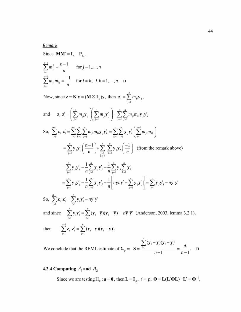
44

Remark

Since ,nn′ = − 1MM Ι Ρ

12

11

1

1 for 1,....,

1 for , , 1,....,

n

jiin

ji kii

nm j nn

m m j k j k nn

−

=

−

=

−= =

−= ≠ =

∑

∑

1Now, since ( ) , then ,

n

p ij

m=

′ = ⊗ =∑z = Κ ji jy M Ι y z y

1 1 1 1and

n n n n

i i ji j ji j ji ki j kj j k j

m m m m= = = =

⎛ ⎞⎛ ⎞′ ′= =⎜ ⎟⎜ ⎟

⎝ ⎠⎝ ⎠∑ ∑ ∑∑z z ′y y y y

1 1 1

1 1 1 1 1 1 1So,

n n n n n n n

i i ji ki j k j k ji kii i k j k j i

m m m m− − −

= = = = = = =

⎛ ⎞′ ′ ′= = ⎜ ⎟⎝ ⎠

∑ ∑∑∑ ∑∑ ∑z z y y y y

1 1, 1

1 1 (from the remark above)n n n

j j j kj j k

k j

nn n= = =

≠

− −⎛ ⎞ ⎛ ⎞′ ′= +⎜ ⎟ ⎜ ⎟⎝ ⎠ ⎝ ⎠

∑ ∑ ∑y y y y

1 1 1 1

1 1 1 1

1 1

1 1

n n n n

j j j j j kj j j k

n n n n

j j j j j j j jj j j j

n n

n n nn n

= = = =

= = = =

′ ′ ′= − −

⎡ ⎤′ ′ ′ ′ ′= − − − = −⎢ ⎥

⎣ ⎦

∑ ∑ ∑ ∑

∑ ∑ ∑ ∑

y y y y y y

′y y y y y y y y y y y y

1

1 1

1 1

So,

and since ( )( ) (Anderson, 2003, lemma 3.2.1),

n n

i i i ii i

n n

i i i ii i

n

n

−

= =

= =

′ ′ ′= −

′ ′ ′= − − +

∑ ∑

∑ ∑

z z y y y y

y y y y y y y y

1

1 1

1

then ( )( ) .

( )( )We conclude that the REML estimate of .

1 1

n n

i i i ii i

n

i ii

p n n

−

= =

=

′ ′= − −

′− −= = =

− −

∑ ∑

∑

z z y y y y

y y y yAΣ S

4.2.4 Computing 1A and 2A

Since we are testing 0H : =μ 0 , then 1 1, , ( ) ,p p − −′ ′= = = =L Ι Θ L L ΦL L Φ

45

1 , ,1 1, 1 1, 1 1, 1 1,

tr( )tr( ) tr( )tr( ), (4.1)p p p p p p p p

if jg if jg if jg if jgi f j g i f j g

i f j g i f j g

A w w= = = = = = = =

≤ ≤ ≤ ≤

= =∑∑∑∑ ∑∑∑∑ΘΦΡ Φ ΘΦΡ Φ Ρ Φ Ρ Φ

2 , ,1 1, 1 1, 1 1, 1 1,

tr( ) tr( ) (4.2)p p p p p p p p

if jg if jg if jg if jgi f j g i f j g

i f j g i f j g

A w w= = = = = = = =

≤ ≤ ≤ ≤

= =∑∑∑∑ ∑∑∑∑ΘΦΡ ΦΘΦΡ Φ Ρ ΦΡ Φ

1 1

2

tr( ) 2 , and tr( ) 2

tr( )tr( ) 2 , (4.3)

if jg

if jg

if jgif jg

if jgif jg

δ δ

δ δ

σ σ

σ σ

− −

− −

= − = −

⇒ =

Ρ Φ Ρ Φ

Ρ Φ Ρ Φ

11 for where , and

0 for if

if p p p

i fi f

δ σ−×

=⎧= =⎨ ≠⎩

Σ

1Wishart [ , 1], and Wishart [ , 1] (Anderson, 2003, corollary 7.2.3).p

pn n n− − −ΣS A Σ∼ ∼

11 22

12 13 -1,

tr ( ) 2

Also, Anderson provided in section 7.3 that the characteristic function of A , A ,...., A ,

2A , 2A ,......, 2A as

2 ,

where with , and

pp

p p

Ni

p

ij p p ij ji

e i

θ θ θ

−

×

⎡ ⎤Ε = − = Ψ⎣ ⎦= =

AΘ Ι ΘΣ

Θ A , 1p pij N n×

= = −A

Finding the moments

For the first moments,

1[A ]ijiji θ

=

∂ΨΕ = ×

∂Θ 0

1 1 121 1 ( ) 2 2 tr ( 2 ) ( 2 )2

N

p p pij

N i i i ii θ

− − −p

=

⎡ ⎤∂= − − − − −⎢ ⎥

∂⎢ ⎥⎣ ⎦ Θ 0

Ι ΘΣ Ι ΘΣ Ι ΘΣ Ι ΘΣ

( 1) for ˆ tr , and hence E[ ]

2( 1) for ii

p ij ijijij

n i jN

n i jσ

σ σσθ

− =⎛ ⎞ ⎧∂ ⎪= =⎜ ⎟ ⎨⎜ ⎟ − ≠∂ ⎪⎩⎝ ⎠

Θ Σ =

For the second moments, 2

22

12 [A A ]if jgif jg

if jgiδ δ

θ θ− −

=

∂ ΨΕ = ×

∂ ∂Θ 0

46

122

1 2 tr ( 2 ) 22

N

p pjg if

N i i ii θ θ

−−

p

=

⎧ ⎫⎡ ⎤⎛ ⎞∂ − ∂⎪ ⎪= − − −⎢ ⎥⎜ ⎟⎨ ⎬⎜ ⎟∂ ∂⎢ ⎥⎪ ⎪⎝ ⎠⎣ ⎦⎩ ⎭ Θ 0

ΘΙ ΘΣ Ι ΘΣ Σ

2 tr tr 2 trp p pjg if jg if

N Nθ θ θ θ

⎛ ⎞ ⎛ ⎞ ⎛∂ ∂ ∂ ∂= +⎜ ⎟ ⎜ ⎟ ⎜⎜ ⎟ ⎜ ⎟ ⎜∂ ∂ ∂ ∂⎝ ⎠ ⎝ ⎠ ⎝

Θ Θ Θ ΘΣ Σ Σ p

⎞⎟⎟⎠

Σ

22 [A A ] ( 1)tr tr 2( 1)trif jgif jg p p p p

if jg if jg

n nδ δ

θ θ θ θ− − ⎛ ⎞ ⎛ ⎞ ⎛∂ ∂ ∂ ∂

⇒ Ε = − + −⎜ ⎟ ⎜ ⎟ ⎜⎜ ⎟ ⎜ ⎟ ⎜∂ ∂ ∂ ∂⎝ ⎠ ⎝ ⎠ ⎝

Θ Θ Θ ΘΣ Σ Σ⎞⎟⎟⎠

Σ

Ε

Cov[A , A ] [A A ] [A ] [A ]if jg if jg if jg⇒ = Ε −Ε

2 2

1 ( 1) tr tr 2( 1)tr2 if jg p p p

if jg if jg

n nδ δ θ θ θ θ− −

⎧ ⎛ ⎞ ⎛ ⎞ ⎛∂ ∂ ∂ ∂⎪⎛ ⎞= − + −⎜ ⎟ ⎜ ⎟ ⎜⎨⎜ ⎟ ⎜ ⎟ ⎜ ⎟ ⎜∂ ∂ ∂ ∂⎝ ⎠ ⎪ ⎝ ⎠ ⎝ ⎠ ⎝⎩

Θ Θ Θ ΘΣ Σ Σ p

⎞⎟⎟⎠

Σ

2 ( 1) tr trp pif jg

nθ θ

⎫⎛ ⎞ ⎛∂ ∂ ⎪− − ⎜ ⎟ ⎜ ⎬⎜ ⎟ ⎜∂ ∂ ⎪⎝ ⎠ ⎝ ⎭

Θ ΘΣ Σ⎞⎟⎟⎠

22( 1) tr2 if jg p p

if jg

nδ δ θ θ− −

⎛ ⎞− ∂ ∂⎛ ⎞= ⎜ ⎟⎜ ⎟ ⎜ ⎟∂ ∂⎝ ⎠ ⎝ ⎠

Θ ΘΣ Σ

2

1

2trˆ ˆCov[ , ] (4.4)

( 1)2

By noticing that tr 2 (

if jg

if jg

p pif jg

if jg

p p ig jf fg ijif jg

n δ δ

δ δ

θ θσ σ

σ σ σ σθ θ

− −

− −

⎛ ⎞∂ ∂⎜ ⎟⎜ ⎟∂ ∂⎝ ⎠⇒ =

−

⎛ ⎞∂ ∂= +⎜ ⎟⎜ ⎟∂ ∂⎝ ⎠

Θ ΘΣ Σ

Θ ΘΣ Σ ), (4.5)

ˆ ˆ Cov[ , ] (4.6)( 1)

ig jf fg ijif jg n

σ σ σ σσ σ

+=

−

Combining expressions (4.1), (4.3), and (4.6), we obtain

21

1 1, 1 1,

22

1 1 1 1

2( 1)

2( 1)2

if jg

if jg

if jg

p p p pig jf fg ij if jg

i f j gi f j g

p p p pig jf fg ij if jg

i f j g

An

n

δ δ

δ δδ δ

σ σ σ σσ σ

σ σ σ σσ σ

− −

= = = =≤ ≤

− −− −

= = = =

+=

−

+=

−

∑∑∑∑

∑∑∑∑

Note In the last expression above for , we divided by1A 22 if jgδ δ− − , and this is true because

the summations repeat ,if jgw 22 if jgδ δ− − times.

47

11 1 1 1

11

p p p pif jg jg if

ig jf fg ijg f j i

An

σ σ σ σ σ σ σ σ= = = =

⇒ = +− ∑∑∑∑

1 1 1 1 1 1 1 1

1 1 1 1

1 1

1 ( ) ( )1

Therefore,

p p p p p p p pif jg jg if

ig jf fg ijf g i j j f g i

p p p p

gf gf fj fjf g j f

n

n

σ σ σ σ σ σ σ σ

δ δ δ δ

= = = = = = = =

= = = =

⎧ ⎫⎛ ⎞ ⎛ ⎞⎛ ⎞ ⎛⎪ ⎪= +⎨ ⎬⎜ ⎟ ⎜ ⎟⎜ ⎟ ⎜− ⎝ ⎠ ⎝⎪ ⎪⎝ ⎠ ⎝ ⎠⎩ ⎭⎧ ⎫

= +⎨ ⎬− ⎩ ⎭

∑∑ ∑ ∑ ∑∑ ∑ ∑

∑∑ ∑∑

⎞⎟⎠

12

1pA

n=

−

Also, 1 1

1 1 1

1

tr( ) tr tr

( )2 , by utilizing expresion (4.5) above (4.7)if ij

p p p pif jg p p p p p

if jg if jg

ig jf fg ij

n

δ δ

σ σ σ σ

σ σ σ σ

− −− − −

− −

⎛ ⎞ ⎛ ⎞∂ ∂ ∂ ∂= =⎜ ⎟ ⎜ ⎟⎜ ⎟ ⎜ ⎟∂ ∂ ∂ ∂⎝ ⎠ ⎝ ⎠

= +

Σ Σ Σ ΣΡ ΦΡ Φ Σ Σ Σ Σ Σ

.

Combining expressions (4.2), (4.6), and (4.7), we obtain

12

1 1, 1 1,

12

1 1 1 1

( ) ( )2

( 1)

( ) ( )2

( 1)2

1 2( 1)

if ij

if ij

if ij

p p p pig jf fg ij ig jf fg ij

i f j gi f j g

p p p pig jf fg ij ig jf fg ij

i f j g

ig jf fgig jf ig jf

An

n

n

δ δ

δ δδ δ

σ σ σ σσ σ σ σ

σ σ σ σσ σ σ σ

σ σ σ σ σ σ σ

− −

= = = =≤ ≤

− −− −

= = = =

+= +

−

+= +

−

= +−

∑∑∑∑

∑∑∑∑

1 1 1 1 1 1 1 1

p p p p p p p pij

i j g f i j g fσ

= = = = = = = =

⎧⎨⎩∑∑∑∑ ∑∑∑∑

1 1 1 1 1 1 1 1

1 1 1 1 1 1 1 1

1 (1)(1) (1)(1)2( 1)

p p p p p p p pig jf fg ij

fg ij fg iji j g f i j g f

p p p p p p p p

if if if ifg f i f i f g jn


δ δ δ δ

= = = = = = = =

= = = = = = = =

⎫+ + ⎬

⎭⎧ ⎫

= + + +⎨ ⎬− ⎩ ⎭

∑∑∑∑ ∑∑∑∑

∑∑ ∑∑ ∑∑ ∑∑

2 2

2

1 ( )2( 1)

( 1Therefore, 1

)

p p p pn

p pAn

= + +−

+

+=

−


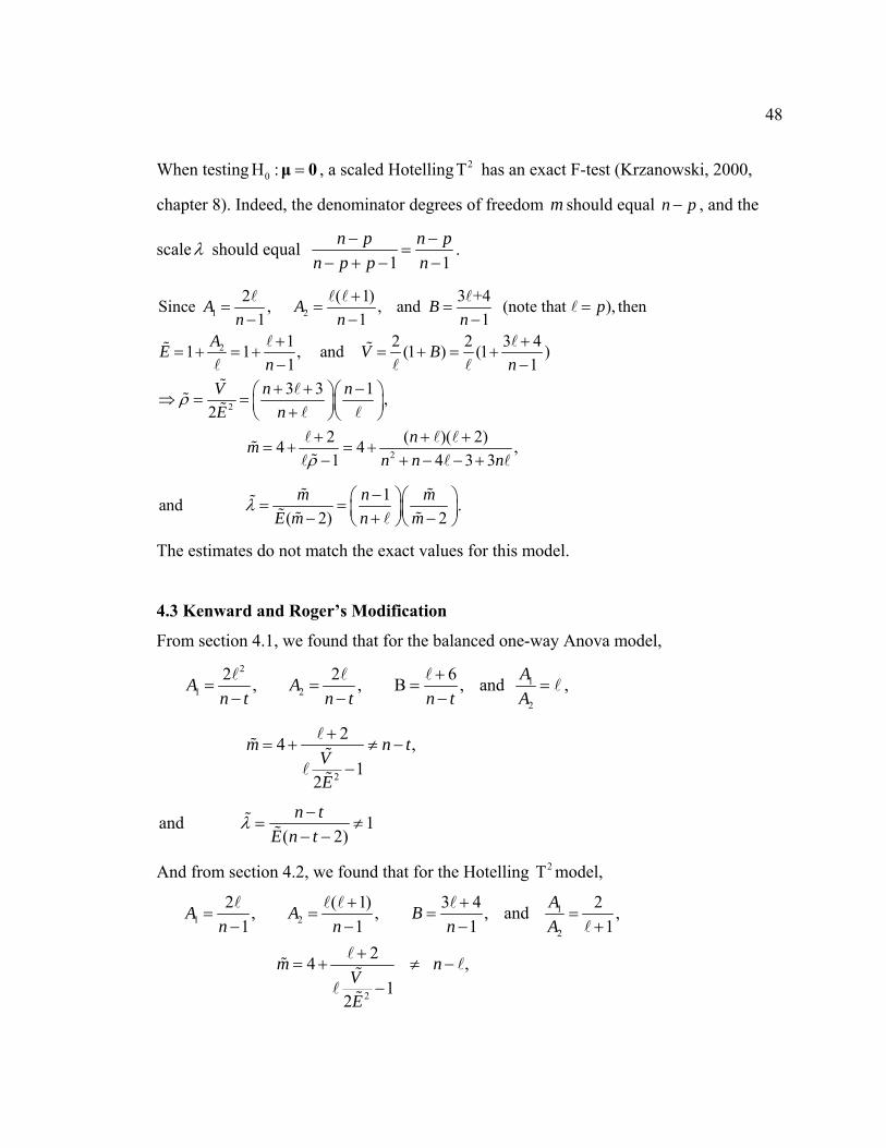
48

When testing 0Η : =μ 0 , a scaled Hotelling has an exact F-test (Krzanowski, 2000, 2Τ

chapter 8). Indeed, the denominator degrees of freedom should equal , and the

scale

m n p−

λ should equal 1 1

n p n pn p p n

− −=

− + − −.

1 2

2

2

2 ( 1) 3 +4Since , , and (note that ), then 1 1 1

1 2 2 3 41 1 , and (1 ) (1 ) 1 13 3 1 ,

22 4

A A B pn n n

AE V Bn n

V n nE n

m

ρ

ρ

+= = = =

− − −+ +

= + = + = + = +− −+ + −⎛ ⎞⎛ ⎞⇒ = = ⎜ ⎟⎜ ⎟+⎝ ⎠⎝ ⎠

+= +

− 2

( )( 2)4 ,1 4 3 3

nn n n

+ += +

+ − − +

1and .( 2) 2

m n mE m n m

λ −⎛ ⎞⎛= = ⎜ ⎟⎜− + −⎝ ⎠⎝⎞⎟⎠

The estimates do not match the exact values for this model.

4.3 Kenward and Roger’s Modification

From section 4.1, we found that for the balanced one-way Anova model,

2

11 2

2

2 2 6, , , and AA An t n t n t A

+= = Β =

− − −= ,

2

2 4 , 1

2

m nV

t

E

+= + ≠ −

−

and 1 ( 2)

n tE n t

λ −= ≠

− −

And from section 4.2, we found that for the Hotelling model, 2Τ

11 2

2

2

2 ( 1) 3 4 , , , and ,1 1 1

2 4 , 1

2

AA A Bn n n A

m nV

21

E

+ += = = =

− − −+

= + ≠ −−

+

49

and .( 2)

n nE n n

λ − −= ≠

− − −1

2

Instead of estimating E[ ] and Var[ ] by and , we will construct modified estimators and leading to

2 4 , 1

2

F F E VE V

mVE

∗ ∗

∗∗

∗

+= +

− (4.8)

and (4.9)( 2)

such that and match the exact values f

mE m

m

λ

λ

∗∗

∗ ∗

∗ ∗

=−

2

or the denominator degrees of freedom and the scale respectively for the balanced one-way Anova and the Hotelling T models.Applying expression (4.9) on the balanced one-way Anova model,

2

2

2

1,( 2)

The expression above, can be rewritten in term as

1,( )

1and hence 1

n tE n t

A

E A

E A

∗

∗

∗

−=

− −

=−

=−

(4.10)

Similarly, applying expression (4.9) on the Hotelling , 2T

2

2

2

,( 2) 1

The expression above, can be rewritten in term of as1

( 1)( 1) ( 1)

1

n nE n n

AA

EA

E

∗

∗

∗

− −=

− − −

=+⎡ ⎤+

− +⎢ ⎥⎣ ⎦

⇒[ ]2

1 ,( 1) ( 1) ( +1)A

=+ − +

2

1and hence (4.11)1

E A∗ =

−

50

From expressions (4.10 and 4.11), we can see that the approximate expression for

should be as E[ ]F

2

1 (4.12)1

E A∗ =

−

Applying expression (4.8) on the balanced one-way Anova model,

2

2

2 41

2The expression above can be rewritten in term as

2 6 4 1

2

n tVE

B

V BE

∗

∗

∗

∗

++ = −

−

+ ++ =

− (4.13)

2

2

2

2

2

2( 2) 6 4,2

2 2 1 .+6 4

Moreover, since for the balanced one-way Anova model,6 2 , and ,

1then 1

EV E B

V E

B

B An t n t

E A

∗

∗ ∗

∗ ∗

∗

+ +⇒ = −

−⎧ ⎫⎛ ⎞⎪ ⎪⎜ ⎟+⎪ ⎪= +⎨ ⎬⎜ ⎟⎪ ⎪⎜ ⎟−⎪ ⎪⎝ ⎠⎩ ⎭

+= =

− −

=−

2

21 , 6

2 6 ( 2)and hence 21 ( 6 4 )

6

B

BVB B

∗

= −+

⎧ ⎫⎪ ⎪+ + −⎪ ⎪= ⎨ ⎬⎛ ⎞⎪ ⎪− + −⎜ ⎟⎪ ⎪+⎝ ⎠⎩ ⎭

2

212 6 , (4.14)

2 41 16 6

by dividing the numerator and the denominator by

B

BB

⎧ ⎫−⎛ ⎞+⎪ ⎪⎜ ⎟⎪ ⎪+⎝ ⎠= ⎨ ⎬⎛ ⎞ ⎛ ⎞⎪ ⎪− −⎜ ⎟ ⎜ ⎟⎪ ⎪+ +⎝ ⎠ ⎝ ⎠⎩ ⎭

6.+

51

Similarly, applying expression (4.8) on the Hotelling model, 2T

2

2 41

2

nVE

∗

∗

++ =

−−

2

The expression above can be rewritten in term as2 3 4 4 1 (4.15)

12

B

V BE

∗

∗

+ ++ = + −

−

2

2

2

2

2

2

2( 2) 3 4 3 ,2

2 2 1 3 +4 3

Moreover, Since for the Hotelling T model,3 4 ( 1) , and ,

1 11then 1

1

EV E B

V E

B

B An n

E A

∗

∗ ∗

∗ ∗

∗

+ +⇒ = − −

−⎧ ⎫⎛ ⎞⎪ ⎪⎜ ⎟+⎪ ⎪= +⎨ ⎬⎜ ⎟⎪ ⎪⎜ ⎟− −⎪ ⎪⎝ ⎠⎩ ⎭

+ += =

− −+

= = −−

2

1 , 3 4

2 3 4and hence .11 [3 4 ( 3

3 4

B

BV) ]B B

∗

+

⎧ ⎫⎪ ⎪+ −⎪ ⎪= ⎨ ⎬

+⎛ ⎞⎪ ⎪− + − +⎜ ⎟⎪ ⎪+⎝ ⎠⎩ ⎭

2

112 3 4 , (4.16)

1 31 13 4 3 4

B

B B

⎧ ⎫−⎛ ⎞+⎪ ⎪⎜ ⎟⎪ ⎪+⎝ ⎠= ⎨ ⎬+ +⎛ ⎞ ⎛ ⎞⎪ ⎪− −⎜ ⎟ ⎜ ⎟⎪ ⎪+ +⎝ ⎠ ⎝ ⎠⎩ ⎭

by dividing the numerator and the denominator by 3 4.+

From expressions (4.14 and 4.16), we can see that the approximate expression for the

variance should be as

12

2 3

12 ,(1 ) (1 )

d BVd B d B

∗ ⎧ ⎫+= ⎨ ⎬− −⎩ ⎭

52

where

1 1

22 2

3 3

2 16 3 4

2 1for the balanced one-way Anova model, for Hotelling Τ model6 3 4

4 36 3 4

d d

d d

d d

− −⎫ ⎫= =⎪ ⎪+ +⎪ ⎪+⎪ ⎪= =⎬ ⎬+ +⎪ ⎪+⎪ ⎪= =⎪ ⎪+ +⎭ ⎭

So far we obtained a general expression for the variance but not for the coefficients .

First, we determine some simple linear relationship among the that are common

between the two cases

'id s

'id s

( ) The numerator of i 2 numerator of d 1d= −

( The numerator of )ii 3 2numerator of 2 numerator of 2d d 1d= + = − +

( The denominator of where )iii 1' is a linear function of the numerator of ,id s d

2

( 2) 6 for the balanced one-way Anova model,3 4 for the Hotelling T model.

c dc d− + = +

− + = +

Solving the two equations above for and , we have 2 and 3 2,c d c d= − = + and hence

the denominator of 1' 3 2(1 the numerator of )id s d= + − .

The involved in relationships ( ) for both special cases are fixed,

whereas any other , which is involved in the numerator of , is accommodated as a

function of the ratio of .

's , ( ), and ( )i ii iii

1d

1 2 and A A

11 1 2

2

Let the numerator of ( , ) .

Notice that 2 for the balanced one-way Anova model,

Ad g A A a b gA

g

= = + =

= −

2 1 for the Hotelling T model.g = −

21

2

2Since and for the balanced one-way Anova and Hotelling T respectively, 1

then 2,

AA

a b

=+

+ = −2and 1 (4.17)

1a b+ = −

+

53

Solving the equations above, we have

( 1)( 1) 1 4, and .( 1) 2 2 2

a b+ − + += = = −

+ − + +

From the expressions we obtained for both , we have and a b

1

2

A1 4 2 A 2

g + += −

+ +

1 2

2

( 1) ( 4)Therefore, for both special cases.( 2)A Ag

A+ − +

=+

Summary

The Kenward and Roger approach that was derived in section 3.2 will be modified as

2

2 4 , where ,1 2

and such that( 2)

VmE

mE m

ρρ

λ

∗∗ ∗

∗ ∗

∗∗

∗ ∗

+= + =

−

=−

12

12

2 3

1 ,

12and ,(1 ) (1 )

AE

d BVd B d B

−∗

∗

⎛ ⎞= −⎜ ⎟⎝ ⎠⎧ ⎫+

= ⎨ ⎬− −⎩ ⎭

1

2

1 23

2

3 2(1 )

3 2(1 )( 1) ( 4)2 , where .

3 2(1 ) ( 2)

gdg

gdg

A Agd gg A

=+ −−

=+ −

+ − +− += =

+ − +

( )2 2Recall that before the modification, [ ] 1 , and Var[ ] 1 ,AF E F VΕ ≈ = + ≈ = + B

( )1 21where 6 ,2

B A A= +

1 21 1 1 1

and tr( )tr( ), tr( )r r r r

ij i j ij i ji j i j

A w A w= = = =

= =∑∑ ∑∑ΘΦΡ Φ ΘΦΡ Φ ΘΦΡ ΦΘΦΡ Φ

54

4.4 Modifying the Approach with the Usual Variance-Covariance Matrix

Recall that when we used the usual variance-covariance of the fixed effects

estimates in section 3.1.1, we found that Φ

21

2[ ] 1 , and Var[ ] (1 ),SF F BΕ ≈ + ≈ +

2 11 2 2 3

6where , and 2 , 42

S SB S A A S+= = + 1 1 3A A= −

1S

Since for both special cases, 3 20, then and A S= are reduced to respectively,

and hence the modification based on the same two special cases considered for K-R

modification should be analogous to K-R modification derived in section 4.3 (substitute

for respectively). The problematic part about this modification is

that , where there is no clear guide for us to accomplish the modification for .

Simulation studies (as we will see in chapter 8) show that this modification does not

perform well to estimate the denominator degrees of freedom and the scale.

2 and A 1A

1A2 1 and S S 2 and A

3 0A = 3A

55

5. TWO PROPOSED MODIFICATIONS FOR THE KENWARD-ROGER METHOD

As we saw in chapter four, the modification applied by Kenward and Roger was

based on modifying the approximate expressions for the expectation and the variance of

the Wald type statistic so the approximation produces the known values for the

denominator degrees of freedom and the scale for the special cases where the distribution

of is exact. The modification for the approximate expression for the expectation was

relatively simple and direct; whereas the modification applied by Kenward and Roger for

the approximate expression for the variance was more complicated. In fact, the

modification that applied by Kenward and Roger is not unique and is ad-hoc. In this

chapter, we propose two other modifications for Kenward and Roger’s method based on

the same two special cases. The approximate expression for the expectation of is

modified as done by Kenward and Roger (1997); however, instead of modifying the

approximate expression for the variance, we modify other quantities as will be seen

shortly. These two proposed modifications are simpler than the K-R modification both in

computation and in derivation. Moreover, like the K-R method, our proposed

modifications produce the exact values for the denominator degrees of freedom and scale

in the two special cases.

F

F

F

5.1 First Proposed Modification

In order to approximate the F test for the fixed effects, in a model as

described in section 2.1, we use the same form of Wald-type statistic used in K-R

method,

0H : ′ =L β 0

F

1A

1 ˆ ˆˆ( )F −′ ′ ′= β L L Φ L L β .

Define ( )2

2

2 2. Recall that 1 , and 11

2

Ah EV

V B

E

+= = +

−= +

Also, recall that chapter 4, for the balanced one-way Anova model, we had

56

2

11 2

2


+= = Β =

− − −= ,

2

24 4 ,1

2

n tV

m h

E

+= + = + ≠ −

− and 1

( 2)n t

E n tλ −= ≠

− −

And for the Hotelling model, we had 2Τ

11 2

2

2 ( 1) 3 4, , , and ,1 1 1

AA A Bn n n A

+ += = = =

− − −2

1+

2

2 4 4 , and ( 2) 11

2

n nm h nV E n nE

λ+ −= + = + ≠ − = ≠

− − −−

−

In this proposed modification, we keep the modified estimator for E[ ] to be as wasF E∗

1

1 1

derived in section 4.3; however, instead of constructing a modified estimator for Var[ ],

we will construct a modified estimator for , say leading to 4 ,

F

h hm h= +

1

(5.1)such that matches the exact values for the denominator degrees of freedom for the

balanced one-way Anova and t

m2he Hotelling T models.

Applying expression (5.1) on the balanced one way Anova model,

1

1

+6 4 , (from 4.13)

+6 4

hB

hB

+ =

= −

And, applying expression (5.1) on the Hotelling model, 2Τ

1

1

3 +4 4 +(1 ) , (from 4.15)

3 +4 3 .

hB

hB

+ = −

= − −

For both models,

11 0 , (5.2)dh d

B= +

57

where 0

1

4 for the balanced one-way Anova model,

6dd

= − ⎫⎬= + ⎭

and 0 2

1

( 3) for the Hotelling Τ model.

3 4dd

= − + ⎫⎬= + ⎭

Also, notice that can be expressed as a linear function of for both models, that is 1d 0d

1 1 0 2

1 22

1 2

,where 6 4 for the balanced one way Anova model,

3 4 ( 3) for the Hotelling T model.

d a d aa a

a a

= ++ = − +

+ = − + +

Solving the equations above, we have 1 22, and 2.a a= − = − That is

1 0 2 2. (5.3)d d= − + −

Like the discussion we made for K-R modification in section 4.3, we need to distinguish

between the fixed and the one to be considered as a function of the ratio of and .

The in expression 5.3 is a fixed one and the in the expression is considered to be a

1A 2A

0d

function of the ratio of and . 1A 2A

11 2 0

2

2

Let ( , )

4 , for the balanced one way Anova model,2 (3 ) for the Hotelling T model.

1

Ag A A d a bA

a b

a b

= = +

⇒ − = +

− + = ++

Solving the two equations above,

( 1) 14, and 2 2

a b+ += − − =

+ +

10

2

21 2

2

( 1) 1And hence, 42 2

( 1) ( 5 8) (5.4)( 2)

AdA

A AA

⎛ ⎞+ += − − + ⎜ ⎟+ + ⎝ ⎠

+ − + +=

+

Summary

Kenward and Rogers’s approach that was derived in section 3.1 is modified as

58

11 1 1

1

1 02 1 0

21 2

02

4 , and ( 2)

such that2 2(1 ) and ,

where( 1) ( 5 8) 6 (Recall that ).

( 2) 2

mm hE m

dE A h dB

A A Ad BA

λ ∗

∗ −

= + =−

− −= − = +

+ − + + += =

+2 1A

5.2 Second Proposed Modification


described in section 2.1, we use the same form of Wald-type statistic used in K-R

method,

0H : ′ =L β 0

F

1A

1 ˆ ˆˆ( )F −′ ′ ′= β L L Φ L L β .

Recall that chapter 4, for the balanced one-way Anova model, we had

2

11 2

2


+= = Β =

− − −= ,

2

2 4 , where 1 2

Vm n tE

ρρ+

= + ≠ − =−

and 1 ( 2)

n tE n t

λ −= ≠

− −

And for the Hotelling model, we had 2Τ

11 2

2

2 ( 1) 3 4, , , and ,1 1 1

AA A Bn n n A

+ += = = =

− − −2

1+

2 4 , 1

and ( 2) 1

m n

n nE n n

ρ

λ

+= + ≠ −

−− −

= ≠− − −

In this proposed modification, we also keep the modified estimator for

for the Kenward and Roger modification and first proposed modification.

E[ ] to be asF E∗

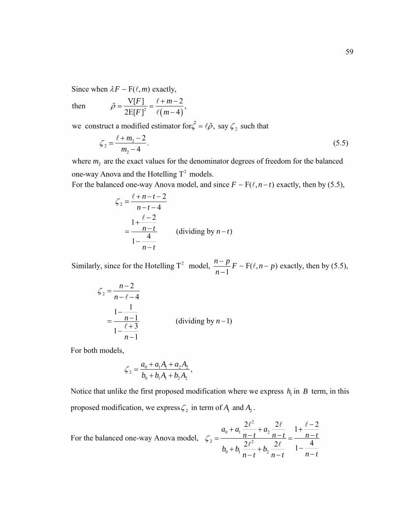
59

( )2

2

22

2

Since when F( , ) exactly, V[ ] 2then ,

2E[ ] 4

we construct a modified estimator for , say such that2 .

4

F mF mF m

mm

λ

ρ

ζ ρ ζ

ζ

+ −= =

−

=+ −

=−

∼

22

(5.5)

where are the exact values for the denominator degrees of freedom for the balanced

one-way Anova and the Hotelling T models.

m

2

For the balanced one-way Anova model, and since F( , ) exactly, then by (5.5),2

421

(dividing by )41

F n tn t

n t

n t n t

n t

ζ

−+ − −

=− −−

+−= −

−−

∼

2Similarly, since for the Hotelling Τ model, F( , ) exactly, then by (5.5),1

n p F n pn−

−−

∼

22

411

1 (dividing by 1)311

nn

n n

n

ζ −=

− −

−−= −+

−−

For both models,

0 1 1 2 22

0 1 1 2 2

, a a A a Ab b A b A

ζ + +=

+ +

Notice that unlike the first proposed modification where we express in 1h B term, in this

proposed modification, we express 2 1in term of and A A2ζ .

For the balanced one-way Anova model,

2

0 1 2

2 2

0 1 2

2 2 1 42 2 1

a a an t n t n t

b b b n tn t n t

ζ

−+ + +

2− − −= =

−+ +−− −

60

20 1 2

20 1 2

, 2 2 ( 2) (5.6)

, 2 2 ( 4)

a c a a c

b c b b c

⇒ = + = −

= + = − (5.7)for any 0c ≠

0 1 22

2

0 1 2

0 1 2

2 ( 1) 111 1 1and for the Hotelling Τ model, 2 ( 1) 311 1 1

, 2 ( 1)

a a an n n

b b bn n n

a c a a c

ζ

++ + −− − −= =

+ ++ + −

− − −⇒ = + + = −

0 1 2

(5.8) , 2 ( 1) ( 3) (5.9)b c b b c= + + = − +

1 2

By solving equations (5.6) and (5.8), we obtain2, and .

2 ( 2) ( 2)c ca a= = −+ +

1 2

By solving equations (5.7) and (5.9), we obtain( 4), and .

( 2) ( 2)c cb b +

= − = −+ +

0 0 1 2 1 2

Take ( 2)

( 2), , 2, 1, ( 4)2

c

a b a a b b

= +

⇒ = = + = = − = − = − +

1 2

21 2

1 2

2 1 2

So, the modification that we apply for will be

( 2) 22 ,

( 2) ( 4)2 ( 2) 2( )24

1 2

A A

A AA A

A A

ζ

ζ

ζ

+ + −=

+ − − ++ + −+

+ =− +

Summary The Kenward and Roger’s approach that was derived in section 3.1 is modified as

1 22

1 2

122 2

2

2 ( 2) 2( ) , 2

and such that (1 ) ( 2)

A AmA A

m E AE m

λ ∗ −∗

+ + −=

+

= = −−

61

5.3 Comparisons among the K-R and the Proposed Modifications

Based on the way we derived K-R and the proposed modifications, we should

expect that these modifications give identical estimates of the denominator degrees of

freedom when the ratio of is the same as one of the ratios for the two special

cases. In this section, we derive some useful results about the three modifications. From

now on, when we say Kenward and Roger’s approach, we mean after the modification

that makes the approach produce the exact values for the two special cases.

1 and A 2A

Theorem 5.3.1 The two proposed and K-R methods give the same estimate of the

denominator degrees of freedom when 1 2 12 or

1 2A A A A= =+

, and the estimate values

are 2 2

2 ( 1), and ( 1) respectively.A A

+− −

Proof For the case where ( )i 1 2A A=

K-R approach

1 2 2 2

2 2

1 2

( 1) ( 4) ( 1) ( 4) 2( 2) ( 2)

2 2 2 4So, , , . 3 2(3 ) 6 6 6

A A A AgA A

d d

+ − + + − += =

+ +− −

= = = =+ − + + +3d

= −

12 1 2

1 6Since (1 ) , and ( 6 ) ,2 2 2E A B A A∗ − A+

= − = + =

21

2 22 3 2 2

2112 2 2then .(1 ) (1 ) (1 ) (1 2 )

Ad BVd B d B A A

∗

−⎧ ⎫+⎪ ⎪⎧ ⎫+= =⎨ ⎬ ⎨− − − −⎩ ⎭

⎬⎪ ⎪⎩ ⎭

2 2

2

2 2

2 21 11 2 2, 1 1 ,2 22 1 1

2

2

22

21

A A AVE A A A

ρ ρ∗

∗ ∗∗

− −⎧ ⎫+ +⎪ ⎪⇒ = = − = − =⎨ ⎬

⎪ ⎪− −⎩ ⎭

+

−

62

22

2

Therefore,2 2 2 4 4 1 . 21

2

m AAAρ

∗∗

+ + ⎛ ⎞= + = + − =⎜ ⎟+− ⎝ ⎠2

First proposed approach 2

1 20

2

01 0

0

22 2

2 2

( 1) ( 5 8) .( 2)2 2 4 ,

2 2 4 1

( 1) ( 5 8) 4 2 ( 2) 4 1( 2) (6 ) (6 )

A AdA

dm dB

dB B

A AA A

+ − + +=

+− −

= + +

−⎛ ⎞= + − +⎜ ⎟⎝ ⎠

⎛ ⎞+ − + +

2A−

= + − +⎜ ⎟+ +⎝ ⎠ +

2 22 2 2

22

3 22

2

2

2 2 2

[ ( 1) ( 5 8) ][(6 ) 4 ] 2 ( 4) 4(6 )( 2)

2 16 24 (4 8)(6 ) 4(6 )( 2)

(4 8)(6 )2 (6 )(2 ) 2 4(6 )( 2) (6 )( 2)

2A A AA

AA

AA A A

+ − + + + − + −= +

+ +

+ + − + += +

+ ++ ++ +

= + − =+ + + +

A

Second proposed approach

1 22

1 2

2 ( 2) 2( ) 2 2

A Am2A A A

+ + −= =

+

( )ii For the case where 1 22

1A A=

+

K-R approach

1 2 1

2 2

1 2 3

( 1) ( 4) ( 1) 4 ( 1) 2 4 1( 2) ( 2) 2 ( 2) 1 2

1 1 3So, , , .3 4 3 4 3 4

A A AgA A

d d d

+ − + + + + += = − = − =

+ + + + + +− + +

= = =+ + +

−

12 1 2

1 4and since (1 ) , and ( 6 ) ,2 (

E A B A A∗ −2

31)

A+= − = + =

+

63

12

2 3

12then (1 ) (1 )

d BVd B d B

∗ ⎧ ⎫+= ⎨ ⎬− −⎩ ⎭

2

22 2

112 ( 1) ,3(1 ) (1 )

( 1)

A

A A

⎧ ⎫−⎪ ⎪+⎪ ⎪= ⎨ ⎬+⎪ ⎪− −+⎪ ⎪⎩ ⎭

22

22

11( 1)1 1( 1) ,3 ( 1) ( 3)1

( 1)

AAV

E AAρ

∗∗

∗

⎧ ⎫−⎪ ⎪ ⎧ ⎫+ −+⎪ ⎪= = =⎨ ⎬ ⎨+ + − +⎩ ⎭⎪ ⎪−+⎪ ⎪⎩ ⎭

⎬

2 2

2 2

2

2 2

( 1) ( 2) 1 1 ,( 1) ( 3) ( 1) ( 3)

and therefore( 1) ( 3)2 ( 4 4 1 ,

1

A AA A

AmA A

ρ

ρ

∗

∗

+ − +− = − =

+ − + + − +

+ − ++ += + = + = − +

−1)

First proposed approach 2

1 20

2

01 0

0

( 1) ( 5 8) ,( 2)

2 2 4

2 2 4 1

A AdAdm d

B

dB B

+ − + +=

+− −

= + +

−⎛ ⎞= + − +⎜ ⎟⎝ ⎠

22 2

2 2

22 2

2 2

2

2 2

2 ( 5 8) 2 ( 1) ( 1)( 2)4 1( 2) (4 3 ) (4 3 )

( 5 6) (4 3 ) 2 ( 1) ( 1)( 2)4( 2) (4 3 ) (4 3 )

(4 3 ) 2 ( 1) ( 1)( 2)4 ( 3)(4 3 ) (4 3 )

A AA A

A AA A

AA A

⎛ ⎞− + + + + −= + − +⎜ ⎟+ + +⎝ ⎠

⎛ ⎞− + + + − +

2

2

A

A+ −

= + +⎜ ⎟+ + +⎝ ⎠⎛ ⎞+ − + + −

= − + +⎜ ⎟+ +⎝ ⎠

2

2

2 2

( 1)( 2) ( 3)[(4 3 ) 2 ( 1)]4(4 3 )

( 1)[2( 3) 2] ( 1)4 ( 3) 1(4 3 )

AA

A A

+ − − + + − += +

++ + + − +

= + − + = − ++

64

Second proposed approach

1 22

1 2 2

2 ( 2) 2( ) ( 1) 1 2

A AmA A A

+ + − += = − +

+

Theorem 5.3.2 1 2 12When or ,

1 2A A A A= =+

then the scale estimates are 1 and

211 respectively for K-R and the proposed modifications as well.

( 1)A−

−+

Proof When , or 1 2A A= 12

1 2A A=+

, the three modifications give the same estimates

for the denominator degrees of freedom which are 2 2

2 and 1A A

+− +

( 1) respectively

(theorem 5.3.1). In addition, since the is modified in the same way for the three

modifications, then the scale estimate is the same for the three modifications. In the

following proof, we use the Kenward and Roger approach to find the scale estimate

E[ ]F

1 22

2

2 2

2( ) For the case where , ,

2

and 1.( 2) 1 2 2

1

i A A mA

AmE m

A A

λ

∗

∗∗

∗ ∗

= =

= =− ⎛ ⎞⎛ ⎞

−⎜ ⎟⎜ ⎟−⎝ ⎠⎝ ⎠

=

1 22

2

2 2

2 ( 1)( ) For the case , 1 ,1

( 1)1and

( 2) 1 ( 1) ( 1)1

ii A A mA

AmE m

A A

λ∗∗

+= = − +

++

− += =

− ⎛ ⎞⎛ +− +⎜ ⎟⎜−⎝ ⎠⎝

⎞⎟⎠

22

2

2

(1 ) 1( 1) , multiplying by

( 1)1 11

AA

AA

−+

+=+⎛ ⎞⎛ ⎞−⎜ ⎟⎜ ⎟− ⎝ ⎠⎝ ⎠

65

2( 1) 1 ( 1)

A−= −

+

Corollary 5.3.3 1 2 12If or ,

1 2A A A A= =+

then the K-R, and the proposed approaches

are identical.

Proof From theorems (5.3.1 and 5.3.2), K-R, and the proposed approaches give the

same estimate of the denominator degrees of freedom and the same estimate for the scale,

and since the statistic used is the same, then all approaches are identical.

Theorem 5.3.4 1 2When 1, then .A A= =

Proof , 11 1

tr( )tr( )r r

ij i ji j

A w= =

=∑∑ ΘΦΡΦ ΘΦΡ Φ 21 1

tr( )r r

ij i ji j

A w= =

=∑∑ ΘΦΡΦΘΦΡ Φ

Since is a scalar, then ,′

′ =′

LLL ΦL ΘL ΦL

1 21 1

1tr( ) tr tr( ) .

and hence, (5.10)( )

i ii i

r ri j

iji j

A w= =

′ ′⎛ ⎞ ′= = =⎜ ⎟′ ′ ′⎝ ⎠′ ′

=′∑∑

LL ΦΡΦ L ΦΡΦLΘΦΡ Φ L ΦΡΦLL ΦL L ΦL L ΦL

L ΦΡΦLL ΦΡ ΦLL ΦL

2

Also,1tr( ) tr( )

( )i j i j′ ′=′

ΘΦΡ ΦΘΦΡ Φ LL ΦΡΦLL ΦΡ ΦL ΦL

2 2

2 21 1

tr( )

( ) ( )

and hence, (5.11)( )

i j i j

r ri j

iji j

A w= =

′ ′ ′ ′= =

′ ′′ ′

=′∑∑

L ΦΡΦLL ΦΡ ΦL L ΦΡΦLL ΦΡ ΦLL ΦL L ΦL

L ΦΡΦLL ΦΡ ΦLL ΦL

From expressions (5.10 and 5.11), we can see that 1 2A A= .

Corollary 5.3.5 the K-R and the proposed approaches are identical. When 1,=

66

The estimates of the denominator degrees of freedom and the scale are2

2 and 1A

respectively.

Proof Since (theorem 5.3.4), then by applying corollary (5.3.3), we have the

K-R and the proposed approaches are identical. By using theorems (5.3.1 and 5.3.2), the

proof is completed.

1A A= 2

67

6. KENWARD AND ROGER’S APPROXIMATION FOR THREE GENERAL MODELS

In chapter 4, we saw how the K-R approach was modified so the approximation

for the denominator degrees of freedom and the scale match the known values for the two

special cases where has an exact F distribution. In this chapter, we show that the K-R

approximation produces the exact values for the denominator degrees of freedom and

scale factor for more general models. Three models are considered: the modified Rady

model which is more general than the balanced one-way Anova model, a general

multivariate linear model which is more general than the Hotelling , and a balanced

multivariate model with a random group effect.

F

2T

6.1 Modified Rady’s Model

A model that satisfies assumptions (A1)-(A5) will be called a Rady model. If the

hypothesis satisfies conditions (A6) and (A7), and the model is a Rady model, the testing

problem will be called a Rady testing problem. Rady (1986) proved that a Rady testing

problem has an exact F test to test a linear hypothesis of the fixed effects. The model

considered in this section is slightly different than Rady’s model where we add two more

assumptions (A8) and (A9) and the model will be called modified Rady’s model. When

the model is a modified Rady model, and the hypothesis satisfies conditions (A6) and

(A7), then the testing problem is called a modified Rady testing problem.

6.1.1 Model and Assumptions

Consider the mixed linear model,

, N( , )y Χβ Σ∼

where 2 21 1 1 1Cov[ ] r r r

2σ σ σ− −= = + + +Σ y Σ Σ Ι iΣ, and are n.n.d. matrices. is a

known matrix, β is a vector of unknown fixed effect parameters, and denotes the set

of all possible vectorsσ and

Χ

ℑ

( ) : .ℵ= ∈Σ σ σ ℑ We are interested in testing 0H : ′ =L β 0 ,

for . an ( ) fixed matrixp′ ×L

68

We assume that the model satisfies assumptions A1-A8 where

(A1) contains an -dimensional rectangle. ℑ r

(A2) ( ) is p.d. for all .Σ σ σ

(A3) and are functionally independent.β σ

(A4) The model has orthogonal block structure (OBS). That is,ℵ is commutative (i.e.

( ) ( ) ( ) ( ) ,∗ ∗ ∗= ∀Σ σ Σ σ Σ σ Σ σ σ σ ∈ℑ ). The orthogonal block structure is equivalent to the

spectral decomposition:

1 1( ) ( ) , where ( ) is a linear function of i.e ( )

i

q r

k k k k k ik iα α α

= =

⎛ ⎞= =⎜ ⎟⎝ ⎠

∑ ∑Σ σ σ Ε σ σ σ α σ , and

's are pairwise orthogonal o.p. matrices.kΕ

(A5) Zyskind’s condition: A model is said to satisfy Zyskind’s condition if

for all . =Χ ΧΡ Σ ΣΡ Σ

(A6) Zyskind’s condition for the submodel under the null hypothesis; for all

where

=U UΣΡ Ρ Σ

Σ ( ) : .′ℜ = =U Χβ L β 0

(A7) ( ) ( ) for some , where , and each can be expressed as where and are symmetric idempotent matrices,with ( ) ),

( ) ( ) and .

s k

k k k k k k

k k k k

sℜ ⊂ℜ = −′= + ℜ ⊂

ℜ =ℜ =

Χ UM B Μ Ρ Ρ EE B C B C C Χ

B E Χ B C 0N(

(A8) ( ) 's are linearly independent.i− ΧΙ Ρ Σ

(A9) . q r=

Remarks

( ) is an o.p.o on ( ), , and notice that ( ) ( ). Then,

( ) is an o.p.o on ( ) ( ) (Seely, 2002, problem, 2.F.3).k k k k k k

k k k k k k

i⊥

ℜ = ℜ ⊂ℜ

= − = − ℜ ℜΧ

Χ

B Ε Χ B Ε Ρ Ε Χ Ε

C Ε B Ε Ι Ρ Ε Ε Χ∩( ) ( ) ( ) )

Proof: Take any ( ) ( )

( ) and ( ) )

k k

k k

k k k

ii ⊥

⊥

⊥

′ℜ ℜ ⊂

∈ℜ ℜ

′⇒ ∈ℜ ∈ℜ =

Ε Ε Χ Χ

x Ε Ε Χ

x Ε x Ε Χ ΧΕ

∩∩

N(

N(

for some , and ., and this means that ).

k k

k k k

′⇒ = =′ ′ ′⇒ = ⇒ = ⇒ = ∈

Ε v x v ΧΕ x 0ΧΕ Ε v 0 ΧΕ v 0 Χ x 0 x ΧN( ′

69

( ) From assumption(A7), ( ) ( ) ( ), and since ( ) ( ),then ( ) ( ), and hence .

s s s

s s

iii ℜ ⊂ℜ =ℜ ℜ ⊂ℜℜ ⊂ℜ =

M B Ε Χ Ε Χ ΕM Ε Ε M M

s

′

ℜ

ˆ( ) Since is estimable, then for some . r( ) r( ) dim[ ( ) )], iv ′ ′= = − ℜL β L Χ A A L A A Χ∩N(

and ( ) ) ( ) ( ) , because ( ) ( ).Therefore, r( ) r( ) r( ) .

⊥′ℜ =ℜ ℜ = ℜ ⊂= = =

A Χ A Χ 0 A ΧL A M

∩ ∩N(

( ) .kv k≠ ∀C 0

1

1 11

1 1

1 1

Proof: Suppose that , then ( )

( ) ( ) ,

and this combined with assumption (A1) implies ( ) 's span ,..., whic

r r

r i i k ki k

r r

i i k ki k

i r

σ α

σ α

−

= =

−

= =

−

= = =

⇒ =

∈

∑ ∑

∑ ∑Χ

Χ

C 0 Σ Σ σ E

Ι -Ρ Σ σ C

Ι -Ρ Σ C C hcontradicts with assumption (A8) that ( ) 's are linearly independent.iΧΙ -Ρ Σ

1 1

1 1 1 1

( ) is invertible.

Proof: Suppose . Then ( ) ( ) ( ) ( )

( ) ( ) ( ) ( ) ( ) ( ) ,

and since ( ) 's are line

ki r rr r

k k k k k kk k

r r r r

k k k k i i i ik k i i

i

vi

k

α

α α α α

α α σ σ

×

∗ ∗ ∗

= =

∗ ∗

= = = =

=

= = ∀ ⇒ =

⇒ − = − ⇒ =

∑ ∑

∑ ∑ ∑ ∑Χ Χ Χ Χ

Χ

B

Bσ Bσ σ σ σ C σ C

Ι Ρ σ E Ι Ρ σ E Ι -Ρ Σ Ι -Ρ Σ

Ι -Ρ Σ arly independent (assumption A8), then .

Hence is injective on , and by assumption (A1), it is injective on , and since it issquare, then it is invertible.

i ir

iσ σ ∗= ∀

ℑB

( )vii The definition of OBS in (A4) was given by Birkes and Lee (2003) which is less

restrictive than the definition given by VanLeeuwen (1998). .et al

Examples

1- Fixed effects linear models which include the balanced one-way Anova model are

modified Rady models.

2- Balanced mixed classification nested models are modified Rady models.

3- Many balanced mixed classification models including balanced split-plot models are

modified Rady models.

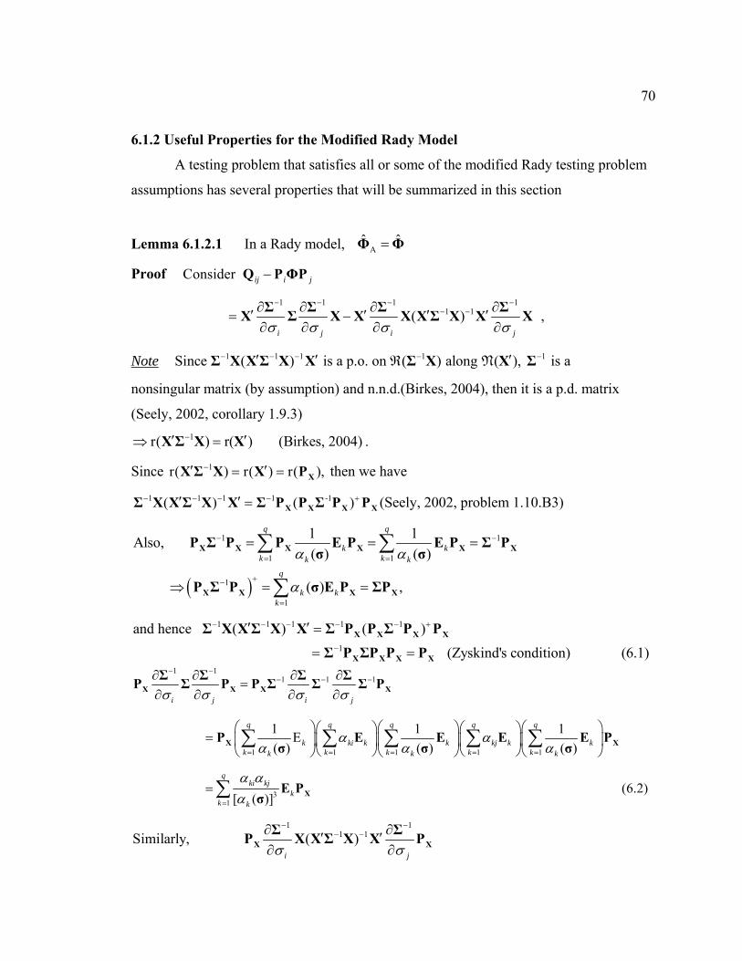
70

6.1.2 Useful Properties for the Modified Rady Model

A testing problem that satisfies all or some of the modified Rady testing problem

assumptions has several properties that will be summarized in this section

Lemma 6.1.2.1 In a Rady model, Aˆ ˆ=Φ Φ

Proof Consider ij i j−Q Ρ ΦΡ

1 1 1 1

1 1 ( ) ,i j i jσ σ σ σ

− − − −− −∂ ∂ ∂ ∂′ ′ ′ ′= −

∂ ∂ ∂ ∂Σ Σ Σ ΣΧ Σ Χ Χ Χ ΧΣ Χ Χ Χ

Note 1 1 1 1 1Since ( ) is a p.o. on ( ) along ( ), is a − − − − −′ ′ ′ℜΣ Χ ΧΣ Χ Χ Σ Χ Χ ΣN

nonsingular matrix (by assumption) and n.n.d.(Birkes, 2004), then it is a p.d. matrix

(Seely, 2002, corollary 1.9.3) 1r( ) r( ) (Birkes, 2004)−′ ′⇒ =ΧΣ Χ Χ .

Since then we have

(Seely, 2002, problem 1.10.B3)

1r( ) r( ) r( ),−′ ′= = ΧΧ Σ Χ Χ Ρ

1 1 1 1 -1( ) ( )− − − − +′ ′ = Χ Χ Χ ΧΣ Χ Χ Σ Χ Χ Σ Ρ Ρ Σ Ρ Ρ

( )

1 1

1 1

1

1

1 1Also, ( ) ( )

( ) ,

q q

k kk kk k

q

k kk

α α

α

− −

= =

+−

=

= =

⇒ = =

∑ ∑

∑

Χ Χ Χ Χ Χ

Χ Χ Χ Χ

Ρ Σ Ρ Ρ Ε Ρ Ε Ρ Σ Ρσ σ

Ρ Σ Ρ σ Ε Ρ ΣΡ

= Χ

1 1 1 1 1

1

and hence ( ) ( )

(Zyskind's condition) (6.1)

− − − − − +

−

′ ′ =

= =Χ Χ Χ Χ

Χ Χ Χ Χ

Σ Χ ΧΣ Χ Χ Σ Ρ Ρ Σ Ρ Ρ

Σ Ρ ΣΡ Ρ Ρ1 1

1 1 1

i j i jσ σ σ σ

− −− − −∂ ∂ ∂ ∂

=∂ ∂ ∂ ∂Χ Χ Χ ΧΣ Σ Σ ΣΡ Σ Ρ Ρ Σ Σ Σ Ρ

1 1 1 1 1

1 1 ( ) ( ) ( )

q q q q q

k ki k k kj k kk k k k kk k

α αα α α= = = = =

⎛ ⎞ ⎛ ⎞ ⎛⎛ ⎞ ⎛ ⎞= Ε⎜ ⎟ ⎜ ⎟ ⎜⎜ ⎟ ⎜ ⎟

⎝ ⎠ ⎝ ⎠⎝ ⎠ ⎝ ⎠ ⎝∑ ∑ ∑ ∑ ∑Χ ΧΡ Ε Ε Ε

σ σ1

k

⎞⎟⎠

Ε Ρσ

31

(6.2)[ ( )]

qki kj

kk k

α αα=

=∑ ΧΕ Ρσ

1 11 1Similarly, ( )

i jσ σ

− −− −∂ ∂′ ′

∂ ∂Χ ΧΣ ΣΡ Χ Χ Σ Χ Χ Ρ

71

1 1 1 1 1 1 ( )i jσ σ

− − − − − −∂ ∂′ ′=∂ ∂Χ ΧΣ ΣΡ Σ Σ Χ ΧΣ Χ ΧΣ Σ Ρ

1 1 i jσ σ

− −∂ ∂=

∂ ∂Χ ΧΣ ΣΡ Σ Ρ Σ Σ Ρ1− Χ

1 1 1 1 1

1 1 ( ) ( ) ( )

q q q q q

k ki k k kj k kk k k k kk k

α αα α= = = = =

⎛ ⎞ ⎛ ⎞ ⎛ ⎞⎛ ⎞ ⎛ ⎞= ⎜ ⎟ ⎜ ⎟ ⎜ ⎟⎜ ⎟ ⎜ ⎟

⎝ ⎠ ⎝ ⎠⎝ ⎠ ⎝ ⎠ ⎝ ⎠∑ ∑ ∑ ∑ ∑Χ ΧΡ Ε Ε Ρ Ε Ε Ε Ρ

σ σ1

kαΧσ

31

(6.3)[ ( )]

qki kj

kk k

α αα=

=∑ ΧΕ Ρσ

From expressions (6.2 and 6.3) we obtain

1 1 1 1

-1 1 ( )i j i jσ σ σ σ

− − − −−∂ ∂ ∂ ∂′ ′− =

∂ ∂ ∂ ∂Χ Χ ΧΣ Σ Σ ΣΡ Σ Ρ Ρ Χ Χ Σ Χ Χ Ρ 0Χ

1 1 1 1-1 1 ( )

i j i jσ σ σ σ

− − − −−∂ ∂ ∂ ∂′ ′ ′ ′⇒ −

∂ ∂ ∂ ∂Σ Σ Σ ΣΧ Σ Χ Χ Χ Χ Σ Χ Χ Χ 0=

This shows that Aˆ ˆ, and since , then . ij i j ij− = = =Q Ρ ΦΡ 0 R 0 Φ Φ

Corollary 6.1.2.2 In balanced mixed classification models, Aˆ ˆ=Φ Φ .

Proof Balanced mixed classification models are Rady models (Rady, 1986), and hence

by applying lemma 6.1.2.1, we have Aˆ ˆ=Φ Φ .

Lemma 6.1.2.3 For a Rady testing problem, 1 2A A= .

Proof : ( ).p= ∈ = ℜΩ Χβ β Χ

0Since we are interested in testing Η : , then is assumed to be estimable( ) ( ) ( ) for some where ,( ) ( ),and hence

: ( ) ( ) ( ).Η

′ ′= ⇔′ ′ ′ ′ℜ ⊂ℜ =ℜ ⇔ = ⇔ = =

ℜ ⊂ℜ′ ′= = =ℜ =ℜ

L β 0 L βL Χ ΧΧ L ΧΧB B L ΧA A ΧBA Χ

Ω Χβ L β 0 Χ A U∩N

Also, since for all (Zyskind's condition for the submodel), and for all (Zyskind's condition), then for all where .

==

= = −

U U

Χ Χ

Χ U

ΣΡ Ρ Σ ΣΣΡ Ρ Σ ΣΣΜ ΜΣ Σ Μ Ρ Ρ

72

1 -1 1 1 1 1 1tr( ) tr ( ) ( ) ( )iiσ

− − − − −⎡ ⎤∂′ ′ ′ ′ ′= − ⎢ ⎥∂⎣ ⎦

ΣΘΦΡ Φ L L ΦL L Χ Σ Χ Χ Σ Σ Χ Χ Σ Χ −

1 -1 1 1 1 -1 tr ( ) ( ) ( )iσ

− − − −⎡ ⎤∂′ ′ ′ ′ ′ ′ ′= − ⎢ ⎥∂⎣ ⎦

ΣΧ A A ΧΦΧA A Χ Χ Σ Χ Χ Σ Σ Χ Χ Σ Χ 1−

1 tr ( ) (from 6.1).iσ

−⎡ ⎤∂′ ′ ′= − ⎢ ⎥∂⎣ ⎦Χ Χ

ΣΡ A A ΧΦΧA A Ρ

1 tr ( ) , because ( ) ( ) iσ

−⎡ ⎤∂′ ′ ′= − ℜ ⊂ℜ⎢ ⎥∂⎣ ⎦

ΣA A ΧΦΧ A A A Χ

1 1 tr ( ) , again notice that iσ

− −⎡ ⎤∂′ ′ ′= − =⎢ ⎥∂⎣ ⎦Χ

ΣA A ΣA A Σ ΧΦΧ Ρ

Since , then is an o.p.o. on ( ) ( )ℜ ⊂ℜU Χ Μ ⊥ΗΩ Ω∩ (Seely, 2002, problem 2.F.3),

[ ]( ) ( ) ( ) ( ) ( ) ( )

( ) ( ) ( ) ( ) ( )So, we have ( ) ( ).

⊥⊥ ⊥Η

⊥

′ ⎡ ⎤= ℜ ℜ =ℜ ℜ +ℜ⎣ ⎦= ℜ ℜ +ℜ ℜ =ℜ

ℜ =ℜ

Ω Ω Χ Χ A Χ Χ A

Χ Χ Χ A AM A

∩ ∩ ∩ ∩

∩ ∩

N

Analogous to the argument given in the proof of lemma 6.2.1, we obtain 1

1

( ) ( ) , (6.4)

and hence, tr( ) tr .iiσ

− +

−

′ ′ = =

⎛ ⎞∂= − ⎜ ⎟∂⎝ ⎠

ΣA A ΣA A ΣM MΣM M M

ΣθΦΡ Φ Σ M

1 11

1 1

1 12

1 1

tr tr ,

tr

r r

iji j i j

r r

iji j i j

A w

A w

σ σ

σ σ

− −

= =

− −

= =

⎛ ⎞⎛ ⎞∂ ∂⇒ = ⎜ ⎟⎜ ⎟ ⎜ ⎟∂ ∂⎝ ⎠ ⎝ ⎠

⎛ ⎞∂ ∂= ⎜ ⎟⎜ ⎟∂ ∂⎝ ⎠

∑∑

∑∑

Σ ΣΣ M Σ M

Σ ΣΣ M Σ M

( ) ( )

1 2

11 1 1 1

and can also be expressed in 's terms as

tr tr , (6.5)( ) ( )

k

q qr rkjki

ij k ki j k kk k

A A

A wαα

α α= = = =

=∑∑ ∑ ∑

Ε

Ε M Ε Mσ σ

And

( )2 21 1 1

tr (6.6)[ ( )]

qr rki kj

ij ki j k k

A wα αα= = =

=∑∑ ∑ Ε Mσ

73

Since (Zyskind's condition for the submodel), then

( ) ( ) ( ), and hence is an o.p.o (Seely, 2002, problem 2.F.1).tr( ) r( ) (Harville, 1997, corollary 10.2.2 and also Seely

k k

k k k

k k

=ℜ =ℜ ⊂ℜ⇒ =

Ε M MΕΕ M MΕ M Ε MΕ M Ε M 's notes).

r( ) dim[ ( ) )] (Seely, 2002, proposition 1.8.2).When , then dim[ ( ) )] 0 (assumption A7),and hence r( ) r( ) (from the remark above).When , then ( ) ( ) (

k

s

k

s k

k s

k s

= − ℜ= ℜ =

= =≠ ℜ ⊂ℜ ⇒ ℜ

M M ΕM Ε

Ε M MM Ε Ε

∩∩N(

N(

) ( ) ( ) ( )k s k k s⊂ ℜ ⇒ℜ ⊂ℜ =M Ε Ε Ε M Ε Ε 0,

and then we have .k =Ε M 0

21 2

1 1

Hence, expressions (6.5) and (6.6) can be simplified as

, [ ( )]

r rsi sj

iji j s

A wα αα= =

=∑∑ σ

2 21 1

and . (6.7)[ ( )]

r rsi sj

iji j s

A wα αα= =

=∑∑ σ

Lemma 6.1.2.4 For a modified Rady model, the approximation and the exact

approaches to derive are identical. REMLˆVar[ ]=W σ

Proof The Exact Approach

122 1

1

1 ( ) (2 ) exp[ ( ) ], N( , )2

1 1( ) constant log ( )2 2

q

R

f π −− −

−

′ ′ ′= −

′ ′ ′⇒ = − −

z Κ ΣΚ z Κ ΣΚ z z 0 Κ ΣΚ

σ Κ ΣΚ z Κ ΣΚ z

∼ ′

11 1 constant log ( ) ,2 2

−′ ′ ′ ′= − −Κ ΣΚ y Κ Κ ΣΚ Κ y

1

1

Since is invertible (from the remarks above) which is equivalent to

( ) a one to one function.

Now, we reparametrize by making ( ), and hence we have

( ) 1 tr ( )2

ki r r

k r

k k

R

k k

α

α

γ α

γ γ

×

×

−

=

=

=

⎡∂ ∂′ ′= −∂ ∂⎣

B

α σ

σ

γ ΣΚ ΣΚ Κ Κ 1 11 ( ) ( )2

1 1 tr , 2 2

k

k k

γ

γ γ

− −⎤ ∂′ ′ ′ ′ ′+⎢ ⎥ ∂⎦⎛ ⎞∂ ∂′= − +⎜ ⎟∂ ∂⎝ ⎠

Σ y Κ Κ ΣΚ Κ Κ Κ ΣΚ Κ y

Σ ΣG y G Gy

74

( )

1 1 -1 1 1 1 1

1

where ( ) ( ) ( ) (from 6.1)( ) 1 1 tr , since

2 2

rR

k k k kkk

γγ

− − − − − −

=

′ ′ ′ ′= − = =

∂ ′⇒ = − + =∂ ∑

ΧG Σ Σ Χ ΧΣ Χ ΧΣ Κ Κ ΣΚ Κ Σ Ι -Ργ GE y GE Gy Σ Ε

12

1

1 1 1 1 tr , since ( )2 2

rk

k kkk kγ γ

−

=

⎛ ⎞′= − + = =⎜ ⎟

⎝ ⎠∑Χ

CC y y G Σ Ι -Ρ Ckγ

( )Equating with zero, R

kγ∂∂

γ REML ˆˆ ( ) , for 1,..., (6.8)kk k

k

k rt

α γ′

= = = y C yσ

1 11 1

REML

REML

ˆ ˆ( ) ( )ˆ ˆ , where

ˆ ˆ( ) ( )

ˆThe above expression is an explicit form for .

k

kr r

t

α α

α α

− −

⎡ ⎤⎡ ⎤ ⎡ ⎤ ⎢ ⎥′⎢ ⎥ ⎢ ⎥ ⎢ ⎥= ⇒ = = =⎢ ⎥ ⎢ ⎥ ⎢ ⎥⎢ ⎥ ⎢ ⎥ ⎢ ⎥⎣ ⎦ ⎣ ⎦

⎣ ⎦

σ σy C yBσ σ B B s s

σ σ

σ

1 1 1REMLˆVar[ ] Var[ ] Var[ ]( ) .

Observe that for any two different elements of ,Cov[ , ] 2tr( ) 4( ) 0 ( Schott, 2005, theorem 10.22).i j i j i j

− − − ′= =

′ ′ ′= + =

σ B s B s Bs

y C y y C y C ΣC Σ Χβ C ΣC Χβ

And

1 1

2

Cov[ , ] 2tr( ) 4( ) 2tr( ),

( ) ( ) ( ) ( )

( )[ ( )] , because 's are orthogonal o.p. matrices

i i i i i i i i

q q

i i i k k i k kk k

i i k

α α

α= =

′ ′ ′= + =

⎛ ⎞ ⎛ ⎞= ⎜ ⎟ ⎜ ⎟

⎝ ⎠ ⎝ ⎠=

∑ ∑Χ Χ

Χ

y C y y C y C ΣC Σ Χβ C ΣC Χβ C ΣC Σ

C ΣC Σ Ι -Ρ Ε σ Ε Ι -Ρ Ε σ Ε

Ι -Ρ σ Ε Ε2 [ ( )]i iα= σ C

2

1 1REML

2[ ( )]So, Var[ ] diag 2 ,

ˆand hence Var[ ] 2 ( ) . (6.9)

i

i r rt

α

×

− −

⎧ ⎫= =⎨ ⎬

⎩ ⎭′=

σs D

σ B D B

The Approximation Approach 1

REML

, 1

ˆVar[ ] 2 tr (Searle ., 1992, P.253),r

i j i jm

et alσ σ

−

=

⎡ ⎤⎧ ⎫⎛ ⎞∂ ∂⎪ ⎪⎢ ⎥= ≈ ⎜ ⎟⎨ ⎬⎜ ⎟⎢ ⎥∂ ∂⎪ ⎪⎝ ⎠⎩ ⎭⎣ ⎦

Σ ΣW σ G G

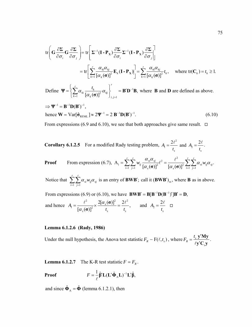
75

1 1tr tr ( ) ( )i j i jσ σ σ

− −⎛ ⎞ ⎡∂ ∂ ∂ ∂

=⎜ ⎟ ⎢ ⎥⎜ ⎟∂ ∂ ∂ ∂⎢ ⎥⎝ ⎠ ⎣Χ Χ

Σ Σ Σ ΣG G Σ Ι -Ρ Σ Ι -Ρσ

⎤

⎦

2 21 1

tr ( ) , where tr( ) 1.[ ( )] [ ( )]

r rki kj ki kj

k kk kk k

t tα α α αα α= =

⎡ ⎤= =⎢ ⎥

⎣ ⎦∑ ∑ΧΕ Ι -Ρ C

σ σ k k= ≥

12

1 , 1

Define , where and are defined as above.[ ( )]

rrk

ki kjk k i j

tα αα

−

= =

⎧ ⎫′= =⎨ ⎬

⎩ ⎭∑Ψ B D B B D

σ

1 1 1

1 1 1REML

( ) ,ˆhence Var[ ] 2 2 ( ) . (6.10)

− − −

− − −

′⇒ =

′= ≈ =

Ψ B D BW σ Ψ B D B

From expressions (6.9 and 6.10), we see that both approaches give same result.

Corollary 6.1.2.5 For a modified Rady testing problem, 2

1 22 2 and

s s

A At t

= = .

Proof 2

21 2 2

1 1 1 1

From expression (6.7), A .[ ( )] [ ( )]

r r r rsi sj

ij si ij sji j i js s

w wα α

α αα α= = = =

= =∑∑ ∑∑σ σ

1 1Notice that is an entry of ; call it ( ) , where as in above.

r r

si ij sj ssi j

wα α= =

′ ′∑∑ BWB BWB B

1 1

22 2

1 22

From expressions (6.9) or (6.10), we have [ ( ) ] ,2[ ( )] 2 2and hence , and

[ ( )]s

s s s s

A At t t

αα

− −′ ′ ′= =

= × = =

BWB B B D B B Dσ

σ

Lemma 6.1.2.6 (Rady, 1986)

Under the null hypothesis, the Anova test statistic , whereF( , )RF ∼ st sR

s

tF′

=′

y Myy C y

.

Lemma 6.1.2.7 The K-R test statistic RF F= .

Proof 1A

1 ˆ ˆˆ ( ) ,F −′ ′ ′= β L L Φ L L β

Aˆ ˆand since (lemma 6.1.2.1), then=Φ Φ

76

1

11 1

1 ˆ ˆˆ ( )

ˆ ˆ( ) ( ) ( )

F

i

−

1 −− − −

′ ′ ′=

⎡ ⎤′ ′ ′= ⎣ ⎦

β L L ΦL L β

L ΦL L ΧΣ Χ L

11 1ˆ ( ) (notice that )−

− −⎡ ⎤′ ′ ′ ′= =⎣ ⎦AΧ ΧΣ Χ ΧA L ΧA

[ ][ ]

1

1

, utilizing expression (6.1)

, because ( ) ( ),

−

−

′=

′= ℜ ⊂

ΧA ΣΡ A

A ΣA A Χℜ

1 1 1 1ˆ ˆ ˆ( ) ( ) ( ) ( utilizing expression 6.1).ii − − − −′ ′ ′ ′= =β Χ Σ Χ Χ Σ y ΧΧ Χ y

[ ]

[ ]

[ ]

11 1

1

1

1

From ( ) and ( ), 1 ( ) ( )

1

1 (because ( ) ( ))

1 ˆ (utilizing expression 6.4),

i ii

F −− −

−

−

−

′ ′ ′ ′ ′ ′ ′=

′ ′ ′=

′ ′ ′= ℜ

′=

Χ Χ

y Χ ΧΧ ΧA A ΣA A Χ ΧΧ Χ

⊂ℜ

y

y Ρ A A ΣA A Ρ y

y A A ΣA A y A Χ

y Σ My

1

1

1 1ˆbut (from the remarks of this section),ˆ ˆ( ) ( )

ˆwhere ( ) (from expression 6.8).

Therefore,

q

kk k s

ss

s

sR

s

ttF F

α α

α

−

=

= =

′=

′= =

′

∑Σ M Ε M Mσ σ

y C yσ

y Myy C y

6.1.3 Estimating the Denominator Degrees of Freedom and the Scale Factor 2

11 2

2

2

2 2From corollary, 6.1.2.5, , and , and then .

By utilizing theorems (5.3.1 and 5.3.2) and corollary (5.3.3), K-R and our proposed2approaches are identical. , and

s s

s

AA At t A

m tA

∗

= = =

= = 1.λ∗ =

The estimates of the denominator degrees of freedom and the scale factor match the exact

77

values for the Anova test in lemma 6.1.2.6. So, the K-R approach produces the exact

values for the modified Rady model which is more general than the balanced one-way

Anova model which is one of the special cases considered in modifying the K-R

approach.

6.2 A General Multivariate Linear Model

This model was studied by Mardia (1992) where they show that for this

model, we have an exact F test to test a linear hypothesis of the fixed effects.

.et al

6.2.1 The Model Setting

Consider the model defined by

,= +Y ΧB U

where ( ) is an observed matrix of response variables on each of individuals, ( ) is the design matrix, ( ) is a matrix of unknown parameters, and is a

matrix of unobserved random distu

n p p nn q q p

×× ×

YΧ B U

rbances whose rows for given are uncorrelated. Wealso assume that is a data matrix from N (0, ).p p

ΧU Σ

1 1 (1)

( )

, , ,

's are 1 vectors , and 's and 's are 1 vectors.

p

n p

n n q p

i i iq p

′ ′ ′⎡ ⎤ ⎡ ⎤⎡ ⎤ ⎡ ⎤⎢ ⎥ ⎢ ⎥⎢ ⎥ ⎢ ⎥= = = = =⎢ ⎥ ⎢ ⎥⎢ ⎥ ⎢ ⎥⎢ ⎥ ⎢ ⎥′ ′ ′⎢ ⎥ ⎢ ⎥⎣ ⎦ ⎣ ⎦ ⎣ ⎦ ⎣ ⎦

× ×

y x β Σ 0Y Χ B Σ Ι

y x β 0 Σ

x y β

⊗Σ

Suppose that we are interested in testing: 0Η : ,′ =c BM 0

where (1 ), and ( ) are given matrices , and have a rank .q p r× ×c M M r

Note A special case of this general model is the Hotelling one sample test, in which 2T

, , 1, . So, , and 1n p p r q′= = = = = =Χ 1 B μ c M Ι . Also, the Hotelling two samples is a

special case of this model.

Other Setting

To compute the Wald statistic for our problem so we are able to compute the

estimates of the Kenward and Roger method, we rearrange as a vector. Y

78

1 (1)

( )

,

and are 1 and 1 vectors respectively.Notice that the design matrix for the new setting will be .

n q

p

np pq∗

⎡ ⎤⎡ ⎤⎢ ⎥⎢ ⎥= = ⎢ ⎥⎢ ⎥⎢ ⎥⎢ ⎥⎣ ⎦ ⎣ ⎦

× ×

= ⊗

y βy β

y β

y βΧ Χ Ι

0

(1) (1)

1 1

( ) ( )

The testing problem Η : ,

which is .q q

q q

c c c c

′ =

′ ′⎡ ⎤ ⎡ ⎤⎢ ⎥ ⎢ ⎥⎡ ⎤ ⎡ ⎤= =⎢ ⎥ ⎢ ⎥⎣ ⎦ ⎣ ⎦⎢ ⎥ ⎢ ⎥′ ′⎣ ⎦ ⎣ ⎦

c BM 0

β β MM 0

β β M

(1)

( ) ( ) 11 1

( )

0

,

which is can be written as Η : , where .

q q

j j j j qj j

q

c c c c= =

⎡ ⎤⎢ ⎥′ ′ ′ ′⎡ ⎤⇔ = ⇔ = ⇔ ⎢ ⎥⎣ ⎦⎢ ⎥⎣ ⎦

′ = = ⊗

∑ ∑β

β M 0 M β 0 M Mβ

L β 0 L c M

= 0

So under this setting, 11( ) ( )( )p n p p

−−′⎡ ⎤= ⊗ ⊗ ⊗⎣ ⎦Φ Χ Ι Ι Σ Χ Ι

( ) 11 1

1 1

1

( ) ,

( ) ( )(( )

( ) ,

p p

p p n

p

−− −

− −

−

′ ′= ⊗ = ⊗

′ ′⎡ ⎤= ⊗ ⊗ ⊗⎣ ⎦′ ′⎡ ⎤= ⊗⎣ ⎦

ΧΧ Σ ΧΧ Σ

β ΧΧ Σ Χ Ι Ι Σ p y

ΧΧ Χ Ι y

111 1

1

( )and ( ) ( )(( ) )( ) .

( )p

p

−−− −

−

′′ ′ ′ ′⎡ ⎤= ⊗ ⊗ ⊗ =⎣ ⎦ ′ ′

M Σ ML ΦL c M ΧΧ Σ c M

c ΧΧ c

6.2.2 Useful Properties for the Model

In this section, we derive several lemmas to summarize the useful properties for

this model under the specified testing problem.

Lemma 6.2.2.1 (Mardia et al., 1992, chapter 6) 1 1 1

M 1

ˆ( ) ( ) ( ) ˆLet , where is the REML estimator( ) ( )

ppF

n q

− − −

−

′ ′ ′ ′ ′ ′ ′=

′ ′−

c ΧΧ Χ YM M Σ M M Y Χ ΧΧ cΣ

c ΧΧ c

79

M ,for . Under the null hypothesis, [ ( 1)]F .p r n q rF r n q r − − +1− − +Σ ∼

Note Similar to lemma 4.2.3, 1

( )( )ˆ

n

i ii

p n q=

′− −=

−

∑ y y y yΣ

Special Notation Since ( 1)2

( )p pif i fσ × +=σ ≤

,

, then like in the Hotelling case, we use

the notation .

2T

, ,if jgΡ Ρ , ,, , and if jg if jg if jgwQ R

Lemma 6.2.2.2 . Aˆ ˆ=Φ Φ

Proof 1 1

( ) ( )p pif p n p

if ifσ σ

− −⎛ ⎞∂ ∂′ ′= ⊗ ⊗ ⊗ = ⊗⎜ ⎟⎜ ⎟∂ ∂⎝ ⎠

Σ ΣΡ Χ Ι Ι Χ Ι Χ Χ

1 11( )p p

if jg pif jgσ σ

− −−

⎛ ⎞ ⎛∂ ∂′ ′ ′⎡ ⎤⇒ = ⊗ ⊗ ⊗⎜ ⎟ ⎜⎣ ⎦⎜ ⎟ ⎜∂ ∂⎝ ⎠ ⎝

Σ ΣΡ ΦΡ ΧΧ ΧΧ Σ ΧΧ

⎞⎟⎟⎠

1 1

,p pp

if jgσ σ

− −∂ ∂′= ⊗

∂ ∂

Σ ΣΧΧ Σ

1 1

,

1 1

, ,

( ) ( ) ( )

ˆ ˆ, and since , then we conclude that .

p pif jg p n n p n p

if jg

p pp

if jg

if jg if jg if jg

σ σ

σ σ

− −

− −

⎛ ⎞ ⎛ ⎞∂ ∂′= ⊗ ⊗ ⊗ ⊗ ⊗⎜ ⎟ ⎜ ⎟⎜ ⎟ ⎜ ⎟∂ ∂⎝ ⎠ ⎝ ⎠∂ ∂

′= ⊗∂ ∂

⇒ − = = =

Σ ΣQ Χ Ι Ι Ι Σ Ι Χ Ι

Σ ΣΧΧ Σ

Q Ρ ΦΡ 0 R 0 Φ ΦA

Lemma 6.2.2.3 The K-R test statistic MrF F

n q=

−.

Proof 1A

1 ˆ ˆˆ( )F −′ ′ ′= β L L Φ L L β

( )

1

11 1

1

1 ˆ ˆˆ ( ) (lemma 6.2.2.2)

ˆ( )1 ( ) ( ) ( ) ( )( )

pp p

−

−− −

−

′ ′ ′=

′′′ ′ ′ ′ ′ ′⎡ ⎤ ⎡ ⎤= ⊗ ⊗ ⊗ ⊗⎣ ⎦ ⎣ ⎦′ ′

β L L ΦL L β

M Σ MΧΧ Χ Ι y c M c M ΧΧ Χ Ι y

c ΧΧ c

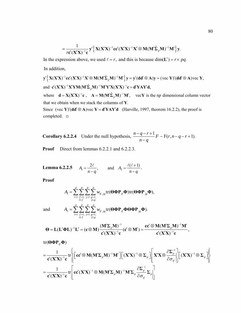
80

1 1 11

1 ˆ ( ) ( ) ( ) . ( )

In the expression above, we used , and this is because dim( ) .

prr r

− − −−

′ ′ ′ ′ ′ ′ ′= ⊗′ ′

′= =

y Χ ΧΧ cc ΧΧ Χ M M Σ M M yc ΧΧ c

L pq×

In addition,

1 1 1

1 1 1

1 1

ˆ( ) ( ) ( ) ( ) (vec ) ( )vec ,

ˆand ( ) ( ) ( ) ,ˆwhere ( ) , ( ) , vec is the dimensional column

p

p

p np

− − −

− − −

− −

′ ′ ′ ′ ′ ′ ′ ′ ′ ′ ′⊗ = ⊗ = ⊗

′ ′ ′ ′ ′ ′ ′ ′ ′=

′ ′ ′= =

y Χ ΧΧ cc ΧΧ Χ M M Σ M M y y dd A y Y dd A Y

c ΧΧ ΧYM M Σ M M Y Χ ΧΧ c d YAY d

d Χ ΧΧ c A M M Σ M M Y vector

that we obtain when we stack the columns of .Since (vec ) ( )vec (Harville, 1997, theorem 16.2.2), the proof is completed.

′ ′ ′ ′⊗ =Y

Y dd A Y d YAY d

Corollary 6.2.2.4 Under the null hypothesis, 1 F( , 1).n q r F r n q rn q

− − +− − +

−∼

Proof Direct from lemmas 6.2.2.1 and 6.2.2.3.

Lemma 6.2.2.5 1 22 (, and A A

n q n q1)+

= =− −

.

Proof

1 ,1 1, 1 1,

2 ,1 1, 1 1,

tr( )tr( ),

and tr( ).

p p p p

if jg if jgi f j g

i f j g

p p p p

if jg if jgi f j g

i f j g

A w

A w

= = = =≤ ≤

= = = =≤ ≤

=

=

∑∑∑∑

∑∑∑∑

ΘΦΡ Φ ΘΦΡ Φ

ΘΦΡ ΦΘΦΡ Φ

1 1

11 1

( ) ( )( ) ( ) ( )

( ) ( )p p

− −−

− − ,′ ′ ′⊗

′ ′ ′ ′= = ⊗ ⊗ =′ ′ ′ ′

M Σ M cc M M Σ M MΘ L L ΦL L c M c M

c ΧΧ c c ΧΧ c′

11 1 1

1

11 1

1

tr( )

1 tr ( ) ( ) ( )( )

1 tr ( ) ( )( )

if

pp p

if

pp p p

if

σ

σ

−− − −

−

−− −

−

⎧ ⎫⎡ ⎤∂⎪ ⎪′ ′ ′ ′ ′ ′⎡ ⎤ ⎡ ⎤ ⎡ ⎤= ⊗ ⊗ ⊗⎢ ⎥⎨ ⎬⎣ ⎦ ⎣ ⎦ ⎣ ⎦′ ′ ∂⎢ ⎥⎪ ⎪⎣ ⎦⎩ ⎭⎡ ⎤∂

′ ′ ′ ′= ⊗⎢ ⎥′ ′ ∂⎢ ⎥⎣ ⎦

ΘΦΡ Φ

Σcc M M Σ M M ΧΧ Σ ΧΧ ΧΧ Σ

c ΧΧ c

Σcc ΧΧ M M Σ M M Σ Σ

c ΧΧ c

p⊗

81

1tr ( ) pp

ifσ−

⎡ ⎤∂′ ′= − ⎢ ⎥

∂⎢ ⎥⎣ ⎦

ΣM M Σ M M

1

1 11 ,

1 1, 1 1,

12 ,

Accordingly, A can be expressed as

tr ( ) tr ( ) ,

and similarly,

tr ( ) (

p p p pp p

if jg p pi f j g if jg

i f j g

pif jg p

if

A w

A w

σ σ

σ

− −

= = = =≤ ≤

−

⎡ ⎤ ⎡ ⎤∂ ∂′ ′ ′ ′= ⎢ ⎥ ⎢ ⎥

∂ ∂⎢ ⎥ ⎢ ⎥⎣ ⎦ ⎣ ⎦

∂′ ′=

∂

∑∑∑∑Σ Σ

M M Σ M M M M Σ M M

ΣM M Σ M M M 1

1 1, 1 1,

) .p p p p

pp

i f j g jgi f j g

σ−

= = = =≤ ≤

⎡ ⎤∂′ ′⎢ ⎥

∂⎢ ⎥⎣ ⎦∑∑∑∑

ΣM Σ M M

1Let ( ) . Since is a symmetric matrix, thenp ij p pt−×′ ′ = =M M Σ M M Τ Τ

for tr

2 for iip

ifif

t it iσ

=⎛ ⎞∂ ⎧⎪=⎜ ⎟ ⎨⎜ ⎟ ≠∂ ⎪⎩⎝ ⎠

ΣΤ

ff

1 1 for Or, tr 2 , where (6.11)

0 for ifp

if ifif

i ft

i fδ δ

σ−⎛ ⎞∂ =⎧

= =⎜ ⎟ ⎨⎜ ⎟ ≠∂ ⎩⎝ ⎠

ΣΤ

1It's easy to check that tr 2 ( ) (6.12)if jgp pig jf jg ij

if jg

t t t tδ δ

σ σ− −⎛ ⎞∂ ∂

= +⎜ ⎟⎜ ⎟∂ ∂⎝ ⎠

Σ ΣT T

2

,

Moreover, analogous to the proof given for expression (4.6) in the Hotelling Τ case,

ˆ ˆ Cov[ , ] ( )

ig jf fg ijif jg if jgw

n qσ σ σ σ

σ σ+

= =−

(6.13)

Utilizing expressions (6.11) and (6.13),

21

1 1, 1 1,

1 1 1 1

2( )

( )

if jgp p p p

ig jf fg ijif jg

i f j gi f j g

p p p pig jf fg ij

if jgi f j g

A t tn q

t tn q

δ δσ σ σ σ

σ σ σ σ

− −

= = = =≤ ≤

= = = =

+=

−

+=

−

∑∑∑∑

∑∑∑∑

Note In the expression above for , we divided by1A 22 if jgδ δ− − , and this is true because

the summations repeat ,if jgw 22 if jgδ δ− − times.

11 1 1 1 1 1 1 1

1 p p p p p p p p

ig if jf jg fg jg ij iff g i j j i g f

A t t tn q

σ σ σ σ= = = = = = = =

⎧ ⎫⎛ ⎞ ⎛ ⎞⎛⎛ ⎞⎪ ⎪⇒ = +⎨ ⎬⎜ ⎟ ⎜ ⎟⎜⎜ ⎟− ⎝ ⎠⎪ ⎪⎝ ⎠ ⎝ ⎠⎝⎩ ⎭∑∑ ∑ ∑ ∑∑ ∑ ∑ t

⎞⎟⎠

82

1 1 1 1

Notice that tr( ),p p p p

ig if jf jg p pf g i j

t tσ σ= = = =

⎛ ⎞⎛ ⎞=⎜ ⎟⎜ ⎟

⎝ ⎠⎝ ⎠∑∑ ∑ ∑ TΣ TΣ

1

1

and since ( ) is o.p. on ( ), then ,

and tr( ) r( ) r( ) (Seely, 2002, chapter 2).

1 2Hence ( ) .

p p p p p p

p p r

rA r rn q n q

−′ ′= ℜ

= = =

= + =− −

TΣ M M Σ M M Σ M TΣ TΣ TΣ

TΣ TΣ M

(6.14)

=

12

1 1, 1 1,

Similarly, and by utilizing expressions (6.12) and (6.13), ( )

( )2( )

if ijp p p p

ig jf fg ijig jf fg ij

i f j gi f j g

A t tn q

t t δ δσ σ σ σ − −

= = = =≤ ≤

+= +

−∑∑∑∑

1 1 1 1

1 1 1 1 1 1 1 1

( ) ( )

2( )

1 2( )

p p p pig jf fg ij

ig jf fg iji j g f

p p p p p p p p

ig ig jf jf ig fg jf iji j g f i j g f

t t t tn q

t t t tn q

σ σ σ σ

σ σ σ σ

= = = =

= = = = = = = =

+= +

−

⎧= +⎨− ⎩

∑∑∑∑

∑∑∑∑ ∑∑∑∑

1 1 1 1 1 1 1 1

1 1 1 1 1 1 1 1

1 2( )

p p p p p p p p

fg ig ij jf fg fg ij iji j g f i j g f

p p p p p p p p

ig ig jf jf ig fg jf ijg i f j i f g j

t t t t

t t t tn q

σ σ σ σ

σ σ σ σ

= = = = = = = =

= = = = = = = =

⎫+ + ⎬

⎭⎧ ⎛ ⎞⎛

= +⎨ ⎜ ⎟⎜ ⎟− ⎩ ⎝ ⎠⎝

∑∑∑∑ ∑∑∑∑

∑∑ ∑∑ ∑∑ ∑ ∑

1 1 1 1 1 1 1 1

p p p p p p p p

⎞

⎠

fg ig ij jf fg fg ij iji f g j g f j i

t t tσ σ σ σ= = = = = = = =

⎛ ⎞⎛ ⎞+ + ⎬⎜ ⎟⎜ ⎟

⎝ ⎠⎝ ⎠∑∑ ∑ ∑ ∑∑ ∑∑ t

⎫

⎭

=

1 1

Since tr( ) r( ) r( ) p p

jf jf p pf j

t rσ= =

= = =∑∑ TΣ TΣ M

1 1 1 1

2 22

and (from above),

1 ( 1)therefore ( ) . (6.15)2( )

p p p p

fg ig ij jfi f g j

t t r

r rA r r r rn q n q

σ σ= = = =

⎛ ⎞⎛ ⎞=⎜ ⎟⎜ ⎟

⎝ ⎠⎝ ⎠+

= + + + =− −

∑∑ ∑ ∑

6.2.3 Estimating the Denominator Degrees of Freedom and the Scale

11 2

2

2 ( 1) 2 , and , and then (lemma 6.2.2.5).1

Ar r rA An q n q A r

+= = =

− − +

83

By utilizing theorems (5.3.1, 5.3.2) and corollary (5.3.3), K-R and the proposed

approaches are identical,

2

2

( 1)where ( 1) 1 (notice that ), A

1 1 1and 1 1 . ( 1)

r rm r n q r

r r n q rAr r n q n q

λ

∗

∗

+= − − = − − + =

− − − − += − = − =

+ − −

r

The estimates of the denominator degrees of freedom and the scale match the values for

the exact multivariate test in corollary 6.2.2.4. So, the K-R approach produces the exact

values for the general multivariate linear model considered in this section which is more

general that the Hotelling model. 2T

6.3 A Balanced Multivariate Model with a Random Group Effect

This model was studied by Birkes (2006) where he showed that there exists an

exact F test to test a linear hypothesis of the fixed effects under a specific condition as we

will see shortly. In this section, we prove that the K-R and the proposed approaches as

well give the same exact values for the denominator degrees of freedom and the scale.

6.3.1 Model Setting

Suppose an experiment yields measurements on p characteristics of a sample of

subjects, and suppose the subjects are in groups each of size m . The measurements of

the -th characteristic of the

t

k j -th subject in the i -th group is denoted by ( 1,..., , ijky i t=

1,...., , 1,...., )j m k= = p . The experiment is designed so that the j -th subject in each

group is associated with covariatesq ( 1,...., )jlx l q= , not depending on i . The design is

balanced in so far as the groups all have the same size m and the same set of covariates.

Each measurement includes a random group effect and a random subject error . ijky ika ijke

Notation

1 1 1 1

, , , , ,j i

j i

m jq t im

x y

x y

′ ′⎡ ⎤ ⎡ ⎤⎡ ⎤ ⎡ ⎤ ⎡ ⎤⎢ ⎥ ⎢ ⎥⎢ ⎥ ⎢ ⎥ ⎢ ⎥= = = = =⎢ ⎥ ⎢ ⎥⎢ ⎥ ⎢ ⎥ ⎢ ⎥⎢ ⎥ ⎢ ⎥′ ′⎢ ⎥ ⎢ ⎥ ⎢ ⎥⎣ ⎦ ⎣ ⎦ ⎣ ⎦⎣ ⎦ ⎣ ⎦

x Y yΧ x Y Y y

x Y y

1ij

ij

ijp

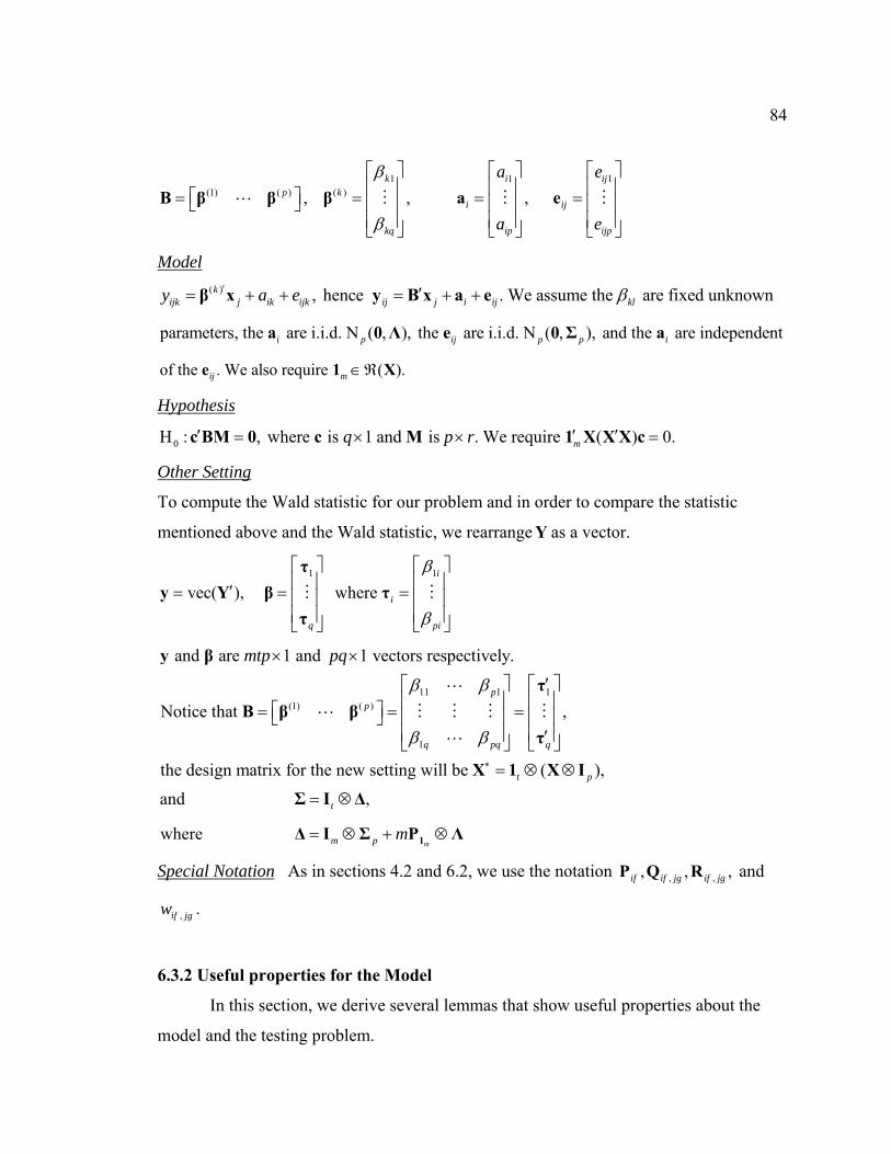
84

1 1(1) ( ) ( ), , ,

k ip k

i ij

kq ip ijp

a e

a e

β

β

1ij⎡ ⎤ ⎡ ⎤ ⎡ ⎤⎢ ⎥ ⎢ ⎥⎡ ⎤= = = ⎢ ⎥=⎢ ⎥ ⎢ ⎥⎣ ⎦ ⎢ ⎥⎢ ⎥ ⎢ ⎥ ⎢ ⎥⎣ ⎦ ⎣ ⎦

B β β β a e

⎣ ⎦

Model( ) , hence . We assume the are fixed unknownk

ijk j ik ijk ij j i ij kly a e β′ ′= + + = + +β x y B x a e

parameters, the are i.i.d. N ( , ), the are i.i.d. N ( , ), and the are independenti p ij p p ia 0 Λ e 0 Σ a

of the . We also require ( ). ij m ∈ℜe 1 Χ

Hypothesis

0 : , where is 1 and is . We require ( ) 0.mq p r′ ′Η = × ×c BM 0 c M 1 Χ ΧΧ c ′ =

Other Setting

To compute the Wald statistic for our problem and in order to compare the statistic

mentioned above and the Wald statistic, we rearrange as a vector. Y

1 1

vec( ), where i

i

q pi

β

β

⎡ ⎤ ⎡ ⎤⎢ ⎥ ⎢ ⎥′= = =⎢ ⎥ ⎢ ⎥⎢ ⎥ ⎢ ⎥⎣ ⎦ ⎣ ⎦

τy Y β τ

τ

11 1 1(1) ( )

1

and are 1 and 1 vectors respectively.

Notice that ,

the design matrix for the new setting will be ( ),

and

pp

q pq q

t p

mtp pq

β β

β β∗

× ×

′⎡ ⎤ ⎡ ⎤⎢ ⎥ ⎢ ⎥⎡ ⎤= = =⎢ ⎥ ⎢ ⎥⎣ ⎦⎢ ⎥ ⎢ ⎥′⎣ ⎦ ⎣ ⎦

= ⊗ ⊗

y β

τB β β

τ

Χ 1 Χ Ι

,t= ⊗Σ Ι Δ

where mm p m= ⊗ + ⊗1Δ Ι Σ Ρ Λ

Special Notation As in sections 4.2 and 6.2, we use the notation and , ,, ,if if jg if jgΡ Q R ,

,if jgw .

6.3.2 Useful properties for the Model

In this section, we derive several lemmas that show useful properties about the

model and the testing problem.

85

Lemma 6.3.2.1 . Aˆ ˆ=Φ Φ

Proof mm p m= ⊗ + ⊗1Δ Ι Σ Ρ Λ

( ) ( )( ) ( )

( ) ( ) 11 1

11 1

,

(6.16)

( ) ( ) ( ) (

m m

m m

m m

m p p

m p p

p p p m p p

m

m

m

−− −

−− −

= − ⊗ + ⊗ +

= − ⊗ + ⊗ +

′ ′⇒ ⊗ ⊗ = ⊗ − ⊗ + ⊗ + ⊗

1 1

1 1

1 1

Ι Ρ Σ Ρ Σ Λ

Δ Ι Ρ Σ Ρ Σ Λ

Χ Ι Δ Χ Ι Χ Ι Ι Ρ Σ Ρ Σ Λ Χ Ι

( ) ( ) 11

11

)

Hence,

( ) ( )( )

m m

p

m p p

t p t t p

m−−

−−

′ ′= − ⊗ + ⊗ +

′⎡ ⎤= ⊗ ⊗ ⊗ ⊗ ⊗⎣ ⎦

1 1Χ Ι Ρ Χ Σ Χ Ρ Χ Σ Λ

Φ 1 Χ Ι Ι Δ 1 Χ Ι

11( ) ( ) p p

t

−−′⎡ ⎤⊗ ⊗⎣ ⎦=Χ Ι Δ Χ Ι

( ) ( )

( ) ( )

111

1 1 1 1

( ) ( ) ( ) ( ) (6.17)

m m

m m

m p p

m p p

m

tm

t

−−−

− − − −

⎡ ⎤′ ′− ⊗ + ⊗ +⎢ ⎥⎣ ⎦=

′ ′ ′ ′ ′ ′− ⊗ + ⊗ +=

1 1

1 1

Χ Ι Ρ Χ Σ ΧΡ Χ Σ Λ

ΧΧ Χ Ι Ρ Χ ΧΧ Σ ΧΧ ΧΡ Χ ΧΧ Σ Λ

1

( ) (if t p t t pifσ

−⎛ ⎞∂′= ⊗ ⊗ ⊗ ⊗ ⊗⎜ ⎟⎜ ⎟∂⎝ ⎠

ΔΡ 1 Χ Ι Ι 1 Χ Ι )

1

1 12

( ) ( )

Hence, ( ) ( ) ( ) ( ).

p pif

if jg p p p pif jg

t

t

σ

σ σ

−

− −

∂′= ⊗ ⊗∂

∂ ∂′ ′= ⊗ ⊗ ⊗ ⊗∂ ∂

ΔΧ Ι Χ Ι

Δ ΔΡ ΦΡ Χ Ι Χ Ι Φ Χ Ι Χ Ι

( )

1 1

,

1 1

1 1

,

( ) ( )

( ) ( ).

( ) ( ) ( ) (

if jg t p t t t t pif jg

p pif jg

if jg if jg p p p pif jg

t

t t

σ σ

σ σ

σ σ

− −

− −

− −

⎛ ⎞ ⎛ ⎞∂ ∂′ ′= ⊗ ⊗ ⊗ ⊗ ⊗ ⊗ ⊗⎜ ⎟ ⎜ ⎟⎜ ⎟ ⎜ ⎟∂ ∂⎝ ⎠ ⎝ ⎠∂ ∂′= ⊗ ⊗∂ ∂

∂ ∂′ ′⇒ − = ⊗ − ⊗ ⊗ ⊗∂ ∂

Δ ΔQ 1 Χ Ι Ι Ι Δ Ι 1 Χ Ι

Δ ΔΧ Ι Δ Χ Ι

Δ ΔQ Ρ ΦΡ Χ Ι Δ Χ Ι Φ Χ Ι Χ Ι )

Consider ( ) ( )p pt ′⊗ ⊗Χ Ι Φ Χ Ι

86

( )( )

( ) ( )( ) ( )

( )

1 1

1 1

1 1 1 1

( ) ( ) ( )

( ) ( ) ( ).

( ) ( ) ( ) ( )

m

m

m m

m m

m m

p m p

p p

m p

m p p

p p

m

m

m

− −

− −

− − − −

′ ′ ′= ⊗ − ⊗

′ ′ ′ ′+ ⊗ + ⊗

′ ′ ′ ′ ′ ′ ′ ′= − ⊗ + ⊗

= − ⊗ + ⊗ +

= − ⊗ + ⊗

1

1

1 1

Χ 1 Χ Χ 1 Χ

Χ 1 1

Χ Ι ΧΧ Χ Ι Ρ Χ ΧΧ Σ

ΧΧ ΧΡ Χ ΧΧ Σ Λ Χ Ι

Χ ΧΧ Χ Ι Ρ Χ ΧΧ Χ Σ Χ ΧΧ ΧΡ Χ ΧΧ Χ Σ Λ

Ρ Ι Ρ Ρ Σ Ρ Ρ Ρ Σ Λ

Ρ Ρ Σ Ρ Σ( )( ) ( ) ( )

(observe that ( ))

( ) ( )m m

m

p p m p p m p

m

t

+ ∈ℜ

′⇒ − ⊗ ⊗ = − ⊗ − − ⊗ = − ⊗1 Χ 1 Χ

Λ 1 Χ

Δ Χ Ι Φ Χ Ι Ι Ρ Σ Ρ Ρ Σ Ι Ρ Σ

p +

1

Moreover, ( ) ( ) ( )p pjg

tσ

−∂′− ⊗ ⊗ ⊗∂ΔΔ Χ Ι Φ Χ Ι Χ Ι p

( ) ( ) ( )

( )( ) ( ) ( )

11

11

( ).m m

m m

ppm p m p

jg jg

ppm m p m p

jg jg

m

m

σ σ

σ σ

−−

−−

⎧ ⎫∂ +∂⎪ ⎪= − ⊗ − ⊗ + ⊗ ⊗⎨ ⎬∂ ∂⎪ ⎪⎩ ⎭

∂ +∂= − − ⊗ + − ⊗ =

∂ ∂

Χ 1 1

Χ 1 Χ 1

Σ ΛΣΙ Ρ Σ Ι Ρ Ρ Χ Ι

Σ ΛΣΙ Ρ Ι Ρ Χ Σ Ι Ρ Ρ Χ Σ 0

, ,ˆ ˆThis implies , and since , then . if jg if jg if jg− = = =Q Ρ ΦΡ 0 R 0 Φ ΦA

Lemma 6.3.2.2 (Birkes, 2006) 1 1

d 1

1

0 d , 2

( ) [ ] ( )( 2)Let .( )

where and ( ) ( ) ( ).

Under H , F .

t t

t

i m t mi

r tm t q r

tm t q r tFr

t

F

− −

−

=

− − − +

′ ′ ′ ′ ′ ′ ′ ′− − − +=

′ ′

= = ⊗ − + − ⊗ −∑ 1 Χ 1 1

c ΧΧ ΧY M M Y QYM M YΧ ΧΧ cc ΧΧ c

Y Y Q Ρ Ι Ρ Ι Ρ Ι Ρ

i i

i

∼

1

m

−

Lemma 6.3.2.3 ( ) 11 1

1

ˆ( ) ( ) . ,

( )ptF

r

−− −

−

′ ′ ′ ′ ′ ′ ′=

′ ′

c ΧΧ Χ Y M M Σ M M YΧ ΧΧ c

c ΧΧ ci i

ˆwhere is the REML estimate of .p pΣ Σ

Proof Since (lemma 6.3.2.1), then under the null hypothesis, Aˆ =Φ Φ

11 ˆ ˆˆ( )F −′ ′ ′= β L L ΦL L β

87

( )( )( ) ( )

1

1 1

ˆ ˆˆ( )

ˆ ˆˆ ˆ ,

t p t

t p t p

i −

− −

′ ′= ⊗ ⊗ ⊗

′ ′ ′ ′= ⊗ ⊗ = ⊗ ⊗

β Φ 1 Χ Ι Ι Δ y

Φ 1 Χ Ι Δ y 1 Φ Χ Ι Δ y

( )

( ) ( ) ( ) ( )

1 1 1 1

1 1

From (6.17),

( ) ( ) ( ) ( )

1 ( ) ( )

m m

m m

p

pm p p

m p p

mt

mt

− − − −

− −

′⊗

′⊗′ ′ ′ ′ ′ ′= − ⊗ + ⊗ +

′ ′ ′ ′= − ⊗ + ⊗ +

1 1

1 Χ 1 Χ

Φ Χ Ι

Χ ΙΧ Χ Χ Ι Ρ Χ ΧΧ Σ ΧΧ Χ Ρ Χ ΧΧ Σ Λ

ΧΧ Χ Ι Ρ Ρ Σ ΧΧ Χ Ρ Ρ Σ Λ

( ) ( ) 1 11 ( ) ( )m mp p m

t− −′ ′ ′ ′= − ⊗ + ⊗Χ 1 1ΧΧ Χ Ρ Ρ Σ ΧΧ Χ Ρ Σ Λ ,+

( ) ( ) ( ) ( ) ( )

( )( ) ( )

1 1 1

11

1 1

and from (6.16), we have1 ( ) ( )

1 ( ) ( )

m m

m m

m m m m

p p p

m p p

m p p

mt

m

t

− − −

−−

− −

′ ′ ′ ′ ′⊗ = − ⊗ + ⊗ + ×

− ⊗ + ⊗ +

′ ′ ′ ′= − − ⊗ + − ⊗

Χ 1 1

1 1

Χ 1 1 Χ 1 1

Φ Χ Ι Δ ΧΧ Χ Ρ Ρ Σ ΧΧ ΧΡ Σ Λ

Ι Ρ Σ Ρ Σ Λ

ΧΧ Χ Ρ Ρ Ι Ρ Ι ΧΧ Χ Ρ Ρ Ρ Σ ( ) 1

p m−

+Σ Λ

( ) ( )

1 1

1

( ) ( )

1 ( )

m m mm p p

p

m

t

− −

−

′ ′ ′ ′+ − ⊗ + +

′ ′= ⊗

1 1 1ΧΧ ΧΡ Ι Ρ Σ Λ Σ ΧΧ Χ Ρ Ι

ΧΧ Χ Ι

1p

− ⊗

1

1 1

1ˆSo, ( ) ,

1 1ˆ ( ) ( ) ( )

t p

t p t

t

t t

−

− −

′ ′ ′= ⊗ ⊗

′ ′ ′ ′ ′ ′ ′ ′ ′ ′ ′= ⊗ ⊗ ⊗ = ⊗ ⊗

β 1 ΧΧ Χ Ι y

L β c M 1 ΧΧ Χ Ι y 1 c ΧΧ Χ M y

( )( )

( )

1 1

1 1

1 1

1 1

( ) 1 ( ) ( ) ( )

( ) ( ) ( )

1 ( ) ( )

( ) ( )

m

m

m

m

m p

p

m p

p

ii

tm

t

− −

− −

− −

− −

′

′ ′ ′ ′ ′= ⊗ − ⊗

′ ′ ′+ ⊗ +

′ ′ ′ ′ ′= − ⊗

′ ′ ′ ′ ′+ ⊗ +

1

1

1

1

L ΦL

c M ΧΧ Χ Ι Ρ Χ ΧΧ Σ

ΧΧ Χ Ρ Χ ΧΧ Σ Λ c M

c ΧΧ Χ Ι Ρ Χ ΧΧ c M Σ M

c ΧΧ ΧΡ Χ ΧΧ c M Σ( ) mΛ M

⊗

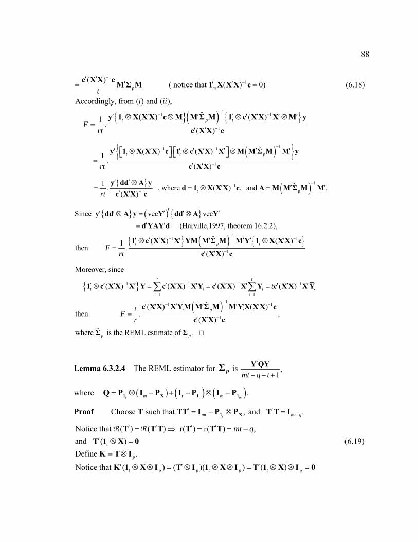
88

( )

11

11 1

1

( ) ( notice that ( ) 0) (6.18)

Accordingly, from ( ) and ( ),

ˆ( ) ( )1 .( )

p m

t p t

ti ii

Frt

−−

−− −

−

′ ′′ ′ ′= =

′ ′ ′ ′ ′ ′ ′ ′⊗ ⊗ ⊗ ⊗=

′ ′

c ΧΧ c M Σ M 1 Χ ΧΧ c

y 1 Χ ΧΧ c M M Σ M 1 c ΧΧ Χ M y

c ΧΧ c

( ) 11 1

1

ˆ( ) ( )1 .( )

t t p

rt

−− −

−

′ ′ ′ ′ ′ ′ ′⎡ ⎤ ⎡ ⎤⊗ ⊗ ⊗⎣ ⎦ ⎣ ⎦=

′ ′

y 1 Χ ΧΧ c 1 c ΧΧ Χ M M Σ M M y

c ΧΧ c

′

( ) 111

1 ˆ . , where ( ) , and .( ) t prt

−−

−

′ ′⊗′ ′ ′= = ⊗ =

′ ′y dd A y

d 1 Χ ΧΧ c A M M Σ M Mc ΧΧ c

( )

( ) 11 1

1

Since vec vec (Harville,1997, theorem 16.2.2),

ˆ( ) ( )1then .( )

t p tF

rt

−− −

−

′′ ′ ′ ′ ′⊗ = ⊗

′ ′=

′ ′ ′ ′ ′ ′ ′ ′⊗ ⊗=

′ ′

y dd A y Y dd A Yd YAY d

1 c ΧΧ Χ YM M Σ M M Y 1 Χ ΧΧ c

c ΧΧ c

( )

1 1 1 1

1 111 1

1

Moreover, since

( ) ( ) ( ) ( )

ˆ( ) ( )then . ,

( )

wher

t t

t i ii i

p

t

tFr

− − − −

= =

−− −

−

′ ′ ′ ′ ′ ′ ′ ′ ′ ′ ′ ′ ′⊗ = = =

′ ′ ′ ′ ′ ′ ′=

′ ′

∑ ∑1 c ΧΧ Χ Y c ΧΧ ΧY c ΧΧ Χ Y c ΧΧ ΧY

c ΧΧ ΧY M M Σ M M YΧ ΧΧ c

c ΧΧ c

i

i i

ˆe is the REML estimate of . p pΣ Σ

Lemma 6.3.2.4 The REML estimator for is pΣ ,1mt q t

′− − +Y QY

where ( ) ( ) ( ).t tm t m= ⊗ − + − ⊗ −1 Χ 1 1Q Ρ Ι Ρ Ι Ρ Ι Ρm

Proof Choose such that , and .tmt mt q−′ ′= − ⊗ =1 ΧΤ ΤΤ Ι Ρ Ρ Τ Τ Ι

Notice that ( ) ( ) r( ) r( ) ,and ( ) (6.19)Define .

Notice that (

t

p

t

mt q′ ′ ′ ′ℜ = ℜ ⇒ = = −′ ⊗ =

= ⊗

′ ⊗ ⊗

Τ Τ Τ Τ Τ ΤΤ 1 Χ 0Κ Τ Ι

Κ 1 Χ ) ( )( ) ( )p p t p t p′ ′= ⊗ ⊗ ⊗ = ⊗ ⊗ =Ι Τ Ι 1 Χ Ι Τ 1 Χ Ι 0

89

[ ]

( )( )

11 1Constant log ( ) ( ) .2 2

Let ( ) ( ) .

( ) ( )

,t

t

R t t

t t

t t mpt p

t p

−′ ′ ′= − ⊗ − ⊗

′ ′ ′= ⊗ = ⊗

′⊗ = ⊗ − ⊗ ⊗

⎡ ⎤= ⊗ − ⊗ ⊗⎣ ⎦

1 Χ

1 Χ

Κ Ι Δ Κ ′y Κ Κ Ι Δ Κ Κ y

D Κ Ι Δ Κ Κ Ι Δ ΚΚΚ

Ι Δ ΚΚ Ι Δ Ι Ρ Ρ Ι

Ι Δ Ρ Δ Ρ Ι

( )where

.m

m

t t m p

mt p t

m

m

⊗ = ⊗ ⊗ + ⊗

= ⊗ + ⊗ ⊗1

1

Ι Δ Ι Ι Σ Ρ Λ

Ι Σ Ι Ρ Λ

( ) ( )

( ) ( )

and

.

Hence, ( ) .

t t m

t t m

t m t

p p

p

t mt p t

m

m

m

⎡ ⎤⊗ ⊗ = ⊗ ⊗ + ⊗⎣ ⎦= ⊗ ⊗ + ⊗ ⊗

′⊗ = − ⊗ ⊗ + ⊗ − ⊗ ⊗

1 Χ 1 Χ 1

1 Χ 1 1

1 Χ 1 1 1

Ρ Δ Ρ Ι Ρ Ρ Σ Ρ Λ

Ρ Ρ Σ Ρ Ρ Λ

Ι Δ ΚΚ Ι Ρ Ρ Σ Ι Ρ Ρ Ρ Λm

( )t′ ′⇒ = ⊗⎡ ⎤⎣ ⎦D Κ Ι Δ ΚΚ Κ

( ) ( ) ( ) ( )( ) ( ) ( )

( ) ( ).

Since from expression (6.19), we have then, .

Also, since ( ), then

t m t m

t m t

t

p mt p t p

p p t

t p

m

m

m m

′= ⊗ − ⊗ ⊗ + ⊗ − ⊗ ⊗ ⊗

⎡ ⎤ ⎡ ⎤ ⎡ ⎤′ ′ ′ ′= ⊗ − ⊗ ⊗ + ⊗ ⊗ − ⊗ ⊗⎣ ⎦ ⎣ ⎦ ⎣ ⎦⎡ ⎤′ ′⊗ = ⊗ ⊗ =⎣ ⎦

′∈ℜ

1 Χ 1 1 1

1 Χ 1 1 1

1 Χ

Τ Ι Ι Ρ Ρ Σ Ι Ρ Ρ Ρ Λ Τ Ι

Τ Τ Σ Τ Ρ Ρ Τ Σ Τ Ι Ρ Τ Λ Τ Ρ Ρ Τ Λ

Τ 1 Χ 0 Τ Ρ Ρ Τ Σ 0

1 Χ ( )

m

( )

1R

.

1 1Hence, Constant log where 2 2

.

t m

mmt q p t

m

m

−

−

⎡ ⎤⊗ ⊗ =⎣ ⎦

′ ′= − −

⎡ ⎤′= ⊗ + ⊗ ⊗⎣ ⎦

1 1

1

Τ Ρ Ρ Τ Λ 0

D y ΚD Κ y

D Ι Σ Τ Ι Ρ Τ Λ

We may re-express D as

( ) ( ) ( )( ) ( ) ( )

( )

11 1

+ , (6.20)

+

Notice that is a p.o., and this is true because

m m

m m

m

mt q t p t p

mt q t p t p

t

t

m

m

−

−− −−

⎡ ⎤ ⎡ ⎤′ ′= − ⊗ ⊗ ⊗ ⊗ +⎣ ⎦ ⎣ ⎦

⎡ ⎤ ⎡ ⎤′ ′= − ⊗ ⊗ ⊗ ⊗ +⎣ ⎦ ⎣ ⎦′ ⊗

′ ⊗

1 1

1 1

1

D Ι Τ Ι Ρ Τ Σ Τ Ι Ρ Τ Σ Λ

D Ι Τ Ι Ρ Τ Σ Τ Ι Ρ Τ Σ Λ

Τ Ι Ρ Τ

Τ Ι Ρ( ) ( ) ( )( )( )( )( ) ( )

m m m t m

m t m m m t m

t t mt t

t t t

′ ′⊗ = ⊗ − ⊗ ⊗

′ ′= ⊗ − ⊗ ⊗ = ⊗ − ⊗

1 1 1 1 Χ 1

1 1 1 1 1 1 1

ΤΤ Ι Ρ Τ Τ Ι Ρ Ι Ρ Ρ Ι Ρ Τ

Τ Ι Ρ Ρ Ρ Ι Ρ Τ Τ Ι Ρ Ρ Ρ Τ

90

( ) ( )

( ) ( ) ( )( )( )

notice that .

Moreover,

r tr trace

tr

m t m

m m m

t m

t

t t t

mt t

′ ′= ⊗ ⊗ =

⎡ ⎤ ⎡ ⎤ ⎡ ⎤′ ′ ′⊗ = ⊗ = ⊗⎣ ⎦ ⎣ ⎦ ⎣ ⎦⎡ ⎤= − ⊗ ⊗⎣ ⎦

1 1 1

1 1 1

1 Χ 1

Τ Ι Ρ Τ Τ Ρ Ρ 0

Τ Ι Ρ Τ Τ Ι Ρ Τ ΤΤ Ι Ρ

Ι Ρ Ρ Ι Ρ

( ) ( ) tr trace 1 (6.21)m t mt t= ⊗ − ⊗ = −1 1 1Ι Ρ Ρ Ρ

( ) ( )1 1mp mt q t

− −−

⎡ ⎤′ ′= ⊗ − ⊗ ⊗⎣ ⎦1ΚD Κ Τ Ι Ι Τ Ι Ρ Τ Σ p

( ) ( ) ( )

( ) ( ) ( )( )

( )

1

11

1

,

where

m

m m

m

t t

t p p

t p t p

t p

mt mt

m

m

−

−−

−

⎡ ⎤′ ′+ ⊗ ⊗ + ⊗⎣ ⎦

⎡ ⎤ ⎡ ⎤′ ′ ′ ′ ′= − ⊗ ⊗ + ⊗ ⊗ +⎣ ⎦ ⎣ ⎦⎡ ⎤′ ′ ′− ⊗ ⊗⎣ ⎦

= − ⊗ − − ⊗

1

1 1

1

1 Χ 1 Χ

Τ Ι Ρ Τ Σ Λ Τ Ι

ΤΤ ΤΤ Ι Ρ ΤΤ Σ ΤΤ Ι Ρ ΤΤ Σ Λ

ΤΤ ΤΤ Ι Ρ ΤΤ Σ

Ι Ρ Ρ Ι Ρ Ρ ( )( ) 1m tt mt p

−⎡ ⎤⊗ − ⊗ ⊗⎣ ⎦1 1 ΧΙ Ρ Ι Ρ Ρ Σ

( ) ( )( ) ( )

1

1

1

,

and

t m t m

m

m t m

mt t p

t p

t p

m

m

−

−

−

⎡ ⎤= − ⊗ − ⊗ − ⊗ ⊗⎣ ⎦

⎡ ⎤′ ′⊗ ⊗ +⎣ ⎦

= ⊗ − ⊗ ⊗ +

1 Χ 1 1 1

1

1 1 1

Ι Ρ Ρ Ι Ρ Ρ Ρ Σ

ΤΤ Ι Ρ ΤΤ Σ Λ

Ι Ρ Ρ Ρ Σ Λ

( ) ( )

1

11

Hence,

Notice that

t m t m m t m

t m t m

t t m t m t

mt t p t p

mt t

m mt t m

m

−

−−

′

⎡ ⎤= − ⊗ − ⊗ + ⊗ ⊗ + ⊗ − ⊗ ⊗ +⎣ ⎦− ⊗ − ⊗ − ⊗

= ⊗ − ⊗ + − ⊗ + ⊗ − ⊗

=

1 Χ 1 1 1 1 1 1

1 Χ 1 1 1

1 1 Χ 1 1 1 1

ΚD Κ

Ι Ρ Ρ Ι Ρ Ρ Ρ Σ Ι Ρ Ρ Ρ Σ Λ

Ι Ρ Ρ Ι Ρ Ρ Ρ

Ρ Ι Ρ Ρ Ι Ι Ρ Ρ Ρ Ρ Ι

( ) ( ) ( )t t mm t m⊗ − + − ⊗ −1 Χ 1 1Ρ Ι Ρ Ι Ρ Ι Ρ

( ) ( )( ) ( ) ( )

11 1 , (6.22)

where .m t m

t t m

p t p

m t m

m−− −′⇒ = ⊗ + ⊗ − ⊗ ⊗ +

= ⊗ − + − ⊗ −

1 1 1

1 Χ 1 1

ΚD Κ Q Σ Ι Ρ Ρ Ρ Σ Λ

Q Ρ Ι Ρ Ι Ρ Ι Ρ

( ) ( )( ) ( ) ( )

Since , , , and are n.n.d. matrices,

so is and , (Harville,

1997, P.369)

m m

m m

t mt q t p p

mt q t p t p

m

m

−

−

′ ′⊗ − ⊗ +

⎡ ⎤ ⎡ ⎤′ ′− ⊗ ⊗ ⊗ ⊗ +⎣ ⎦ ⎣ ⎦

1 1

1 1

Τ Ι Ρ Τ Ι Τ Ι Ρ Τ Σ Σ Λ

Ι Τ Ι Ρ Τ Σ Τ Ι Ρ Τ Σ Λ

91

( )Hence, ,mmt q t p−

⎡ ⎤′ ′− ⊗ ⊗ =⎣ ⎦1Ι Τ Ι Ρ Τ Σ GG

( ) ( )

( ) ( ) ( )

and ,

for some full column rank matrices and (Seely, 2002, Problem 2.D.2).Notice that since

,

then

m

m m

t p

mt q t t p

m

m−

⎡ ⎤′ ′⊗ ⊗ + =⎣ ⎦

⎡ ⎤ ⎡ ⎤′ ′− ⊗ ⊗ ⊗ ⊗ +⎣ ⎦ ⎣ ⎦′ ′ ′ ′= ⇒

1

1 1

Τ Ι Ρ Τ Σ Λ HH

G H

Ι Τ Ι Ρ Τ Σ Τ Ι Ρ Τ Σ Λ = 0

GG HH 0 G G

( ) ( ) ( ).

Hence, m mmt q t t p m−

′ ′= ⇒ =

⎡ ⎤ ⎡ ⎤′ ′− ⊗ ⊗ + ⊗ ⊗ + = +⎣ ⎦ ⎣ ⎦1 1

G HH H 0 G H 0

Ι Τ Ι Ρ Τ Σ Τ Ι Ρ Τ Σ Λ GG HH′ ′

[ ] [ ] , ,′ ′ ′⎡ ⎤ ⎡ ⎤ ′ ′= = = =⎢ ⎥ ⎢ ⎥′ ′ ′⎣ ⎦ ⎣ ⎦

G G G G 0G H G H G G H H

H H 0 H H

( ) ( )1 1

Recall that is a projection operation, and r 1,

and hence, , and .

m mt t

mt q t t

p p

t

m− − + −

⎡ ⎤′ ′⊗ ⊗⎣ ⎦

′ ′= = +

1 1Τ Ι Ρ Τ Τ Ι Ρ Τ

G G Σ H H Σ Λ

= −

( ) ( ) ( )

( )

11 1

1 1R

In addition, by using expression (6.22), we obtain

.

1 1Accordingly, Constant log ( ).2 2

Since and are unstr

m t mp t p

mt q t

p p p

p

m

f m

−− −

− − + −

⎡ ⎤′ ′ ′ ′= ⊗ + ⊗ − ⊗ ⊗ +⎢ ⎥⎣ ⎦

′= − − ⊗ + +

1 1 1 y ΚD Κ y y Q Σ y y Ι Ρ Ρ Ρ Σ Λ y

Σ y Q Σ y Σ Λ

Σ Λ

R

uctured, then and may be considered as different

random variables. This means that to maximize with respect to , it sufficies to

maximize with respect to ,

where

p p

p

R p

R

m

∗

∗

+

=

Σ Σ Λ

Σ

Σ

( )

( ) ( ) ( )

1

1 1

1 1( 1) log .2 2

vec vec

p p

p p

mt q t −

− −

′− − − + − ⊗

′′ ′ ′⊗ = ⊗

Σ y Q Σ y

y Q Σ y Y Q Σ Y

( )( )

1

1

tr (Harville, 1997, theorem 16.2.2).

tr

p

p

−

−

′=

′=

YΣ Y Q

Σ Y QY

( )11 1So, ( 1) log tr ,2 2R pmt q t∗ − ′= − − − + −Σ Σ Y QYp

ˆand hence (Anderson, 2003, lemma 3.2.2). 1p mt q t

′=

− − +Y QYΣ

92

Note We have two expressions for :Q

( ) ( ) ( )( )

,

and

is a p.o. and r( ) 1

t t

m

m t m

t

mt q t

= ⊗ − + − ⊗ −

′ ′ ′= − ⊗

= − − +

1 Χ 1 1

1

Q Ρ Ι Ρ Ι Ρ Ι Ρ

Q ΤΤ ΤΤ Ι Ρ ΤΤ

Q Q

m

Corollary 6.3.2.5 d2 .

1mt t q r F F

mt q t− − − +

=− − +

Proof By combining the results of lemmas (6.3.23) and (6.3.2.4), we obtain

( ) 11 1

1

d

( ) ( )( 1) . ,( )

2and therefore . 1

t mt q tFr

mt t q r F Fmt q t

−− −

−

′ ′ ′ ′ ′ ′ ′ ′− − +=

′ ′

− − − +=

− − +

c ΧΧ ΧY M M Y QYM M YΧ ΧΧ c

c ΧΧ ci i

Corollary 6.3.2.6 Under the null hypothesis,

2 F( ,1

2)mt t q r F r tm t qmt q t

r− − − +− −

− − +− +∼

Proof Direct from lemma 6.3.2.2 and corollary 6.3.2.5.

Lemma 6.3.2.7 For this model, the approximation and the exact approaches to derive

are identical. REMLˆVar[ ]=W σ

Proof Approximation approach

( )11 1( 1) log2 2R pmt q t∗ −′= − − − + − ⊗Σ y Q Σ y,p

111 1( 1)tr

2 2p pR

pif if if

mt q tσ σ

−∗−

⎛ ⎞ ⎛∂ ∂∂ ′= − − − + − ⊗⎜ ⎟ ⎜⎜ ⎟ ⎜∂ ∂⎝ ⎠ ⎝

Σ ΣΣ y Q y,

σ⎞⎟⎟∂ ⎠

1 22 1 1( 1)tr2 2

p p pR

if jg jg if if jg

mt q tσ σ σ σ σ σ

− −∗ ⎛ ⎞ ⎛∂ ∂ ∂∂ ′= − − − + − ⊗⎜ ⎟ ⎜⎜ ⎟ ⎜∂ ∂ ∂ ∂ ∂ ∂⎝ ⎠ ⎝

Σ Σ Σy Q y

1 ⎞⎟⎟⎠

12 1E ( 1)tr2

p pR

if jg jg if

mt q tσ σ σ σ

−∗⎡ ⎤ ⎛ ∂ ∂∂⇒ − = − − + ⎜ ⎟⎢ ⎥ ⎜ ⎟∂ ∂ ∂ ∂⎢ ⎥⎣ ⎦ ⎝

Σ Σ ⎞

⎠

93

( )2 1 2 11 E( ) E( ) tr

2p p

tif jg if jgσ σ σ σ

− −⎧ ⎫⎡ ⎤⎛ ⎞ ⎛ ⎞∂ ∂⎪ ⎪′+ ⊗ + ⊗ ⊗⎢ ⎥⎜ ⎟ ⎜ ⎟⎨ ⎬⎜ ⎟ ⎜ ⎟∂ ∂ ∂ ∂⎢ ⎥⎪ ⎪⎝ ⎠ ⎝ ⎠⎣ ⎦⎩ ⎭

Σ Σ y Q y Q Ι Δ

( ) ( )2 1 2 1

where E( ) E( )p pt p t

if jg if jgσ σ σ σ

− −⎛ ⎞ ⎛ ⎞∂ ∂′ ′ ′ ′⊗ = ⊗ ⊗ ⊗ ⊗⎜ ⎟ ⎜ ⎟⎜ ⎟ ⎜ ⎟∂ ∂ ∂ ∂⎝ ⎠ ⎝ ⎠

Σ Σ y Q y β 1 Χ Ι Q 1 Χ Ι βp⊗

( ) ( ) ( )2 1 2 1

0t t

p pt m t t m

if jg if jgσ σ σ σ

− −⎡ ⎤∂ ∂′ ′ ′ ′ ′= ⊗ − ⊗ + − ⊗ − ⊗⎢ ⎥

∂ ∂ ∂ ∂⎢ ⎥⎣ ⎦1 Χ 1 Χ

Σ Σβ 1 Ρ 1 Χ Ι Ρ Χ 1 Ι Ρ 1 Χ Ι Ρ Χ β =

( )

( )

1 2 12

2 1

1 1E ( 1)tr + tr2 2

Moreover,

p p pRt

if jg jg if if jg

pt

if jg

mt q tσ σ σ σ σ σ

σ σ

− −∗

−

.⎡ ⎤⎡ ⎤ ⎛ ⎞ ⎛ ⎞∂ ∂ ∂∂

⇒ − = − − + ⊗ ⊗⎢ ⎥⎜ ⎟ ⎜ ⎟⎢ ⎥ ⎜ ⎟ ⎜ ⎟∂ ∂ ∂ ∂ ∂ ∂⎢ ⎥ ⎢ ⎥⎣ ⎦ ⎝ ⎠ ⎝ ⎠⎣ ⎦

⎛ ⎞∂⊗ ⊗ =⎜ ⎟⎜ ⎟∂ ∂⎝ ⎠

Σ Σ ΣQ Ι Δ

ΣQ Ι Δ

( ) ( ) ( )

( )

( ) ( ) ( )

2 1 2 1

2 1 2 1

t t m

m

t t m

p pm t m

if jg if jg

t m p t

p pm p t m p

if jg if jg

m

σ σ σ σ

σ σ σ σ

− −

− −

⎡ ⎤∂ ∂⊗ − ⊗ + − ⊗ − ⊗ ×⎢ ⎥

∂ ∂ ∂ ∂⎢ ⎥⎣ ⎦

⊗ ⊗ + ⊗ ⊗

∂ ∂= ⊗ − ⊗ + − ⊗ − ⊗

∂ ∂ ∂ ∂

1 Χ 1 1

1

1 Χ 1 1

Σ ΣΡ Ι Ρ Ι Ρ Ι Ρ

Ι Ι Σ Ι Ρ Λ

Σ ΣΡ Ι Ρ Σ Ι Ρ Ι Ρ Σ

( )

2 1

2 1 2 1 2 1

12

,

and hence,

tr tr( )tr ( 1)tr .

1E ( 1)tr2

pp

if jg

p pt p

if jg if jg if jg

p pR

if jg jg if

mt q t

mt q t

σ σ

σ σ σ σ σ σ

σ σ σ σ

−

− −

−∗

∂= ⊗

∂ ∂

⎡ ⎤⎛ ⎞ ⎛ ⎞ ⎛ ⎞∂ ∂⊗ ⊗ = = − − +⎢ ⎥⎜ ⎟ ⎜ ⎟ ⎜ ⎟⎜ ⎟ ⎜ ⎟ ⎜ ⎟∂ ∂ ∂ ∂ ∂ ∂⎢ ⎥⎝ ⎠ ⎝ ⎠ ⎝ ⎠⎣ ⎦⎡ ⎤ ⎛ ⎞∂ ∂∂

⇒ − = − − + ⎜ ⎟⎢ ⎥ ⎜∂ ∂ ∂ ∂⎢ ⎥⎣ ⎦ ⎝ ⎠

ΣQ Σ

Σ ΣQ Ι Δ Q Σ Σ

Σ Σ

pp

−∂ Σ

2 11+ ( 1)tr .2

pp

if jg

mt q tσ σ

−⎛ ⎞∂− − + ⎜ ⎟⎟ ⎜ ∂ ∂⎝ ⎠

ΣΣ ⎟

2 1 1 11Notice that since ,p p p p p

p pif jg jg if if jgσ σ σ σ σ σ

− − −−

⎛ ⎞∂ ∂ ∂ ∂ ∂= − +⎜ ⎟⎜ ⎟∂ ∂ ∂ ∂ ∂ ∂⎝ ⎠

Σ Σ Σ Σ ΣΣ Σ pΣ

2 1 1

121 1

then, tr 2tr .

1 1E ( 1)tr ( 1)tr2 2

p p pp

if jg jg if

p p p pRp p

if jg jg if jg if

mt q t mt q t

σ σ σ σ

σ σ σ σ σ σ

− −

−∗− −

⎛ ⎞ ⎛ ⎞∂ ∂ ∂= −⎜ ⎟ ⎜ ⎟⎜ ⎟ ⎜ ⎟∂ ∂ ∂ ∂⎝ ⎠ ⎝ ⎠

⎡ ⎤ ⎛ ⎞ ⎛∂ ∂ ∂ ∂∂⇒ − = − − − + = − − +⎜ ⎟ ⎜⎢ ⎥ ⎜ ⎟ ⎜∂ ∂ ∂ ∂ ∂ ∂⎢ ⎥⎣ ⎦ ⎝ ⎠ ⎝

Σ Σ ΣΣ

Σ Σ Σ ΣΣ Σ

⎞⎟⎟⎠

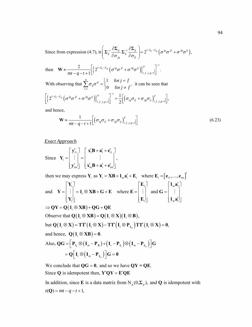
94

( )11 1Since from expression (4.7), tr 2 ,if jgp p ig jf fg ijp p

jg if

δ δ σ σ σ σσ σ

− −− −⎛ ⎞∂ ∂

= +⎜ ⎟⎜ ⎟∂ ∂⎝ ⎠

Σ ΣΣ Σ

( )

( )

11

, , , 1

1

11

, , , 1

2then 2 .1

1 for With observing that , it can be seen that

0 for

122

if jg

if jg

pig jf fg ij

i f j g

pif

iji

pig jf fg ij

ig if fgi f j g

mt q tj fj f

δ δ

δ δ

σ σ σ σ

σ σ


−− −

=

=

−− −

=

⎡ ⎤≈ +⎢ ⎥⎣ ⎦− − +

=⎧= ⎨ ≠⎩

⎡ ⎤+ = +⎢ ⎥⎣ ⎦

∑

W

( ), , , 1

,p

ij i f j g=⎡ ⎤⎢ ⎥⎣ ⎦

( ), , , 1

and hence, 1 (6.23)

1p

ig if fg ij i f j gmt q tσ σ σ σ

=⎡ ⎤≈ +⎢ ⎥⎣ ⎦− − +

W

Exact Approach

[ ]

1 1 1

1

1 1

Since ,

then we may express as where ,....,

and where a

i i i

i

im m i im

i i m i i i i im

t

t t

′ ′ ′ ′+ +⎡ ⎤ ⎡ ⎤⎢ ⎥ ⎢ ⎥= =⎢ ⎥ ⎢ ⎥′ ′ ′ ′⎢ ⎥ ⎢ ⎥+ +⎣ ⎦ ⎣ ⎦

′′= + + =

⎡ ⎤ ⎡ ⎤⎢ ⎥ ⎢ ⎥= = ⊗ + + =⎢ ⎥ ⎢ ⎥⎢ ⎥ ⎢ ⎥⎣ ⎦ ⎣ ⎦

y x B a eY

y x B a e

Y Y ΧB 1 a E E e e

Y EY 1 ΧB G E E

Y E

( )( ) ( )( )

( ) ( ) ( ) ( )( )

( ) ( ) ( )( )

1

nd

Observe that ,

but ,

and hence, .

Also,

m

t t m

m

m

m t

t

t t t

t t t t

t

m t m

t m

′⎡ ⎤⎢ ⎥= ⎢ ⎥

′⎢ ⎥⎣ ⎦⇒ = ⊗ + +

⊗ = ⊗ ⊗

′ ′ ′⊗ = ⊗ − ⊗ ⊗ =

⊗ =

⎡ ⎤= ⊗ − + − ⊗ −⎣ ⎦⎡ ⎤= ⊗ − =⎣ ⎦

1

1 Χ 1 1

1

1 aG

1 a

QY Q 1 ΧB QG QE

Q 1 ΧB Q 1 Χ Ι B

Q 1 Χ ΤΤ 1 Χ ΤΤ Ι Ρ ΤΤ 1 Χ 0

Q 1 ΧB 0

QG Ρ Ι Ρ Ι Ρ Ι Ρ G

Q Ι Ι Ρ G 0

We conclude that , and so we have .Since is idempotent then,

=′ ′=

QG 0 QY = QEQ Y QY E QE

In addition, since is a data matrix from N (0, ), and is idempotent with

r( ) 1, p p

mt q t= − − +

E Σ Q

Q

95

p

2

then W ( , 1) (Mardia, 1992, theorem 3.4.4).

Analogous to the argument given for Hotelling T case in section 4.2.4 that leads toexpression (4.6), we have

p mt q t′ ′= − − +E QE Y QY Σ∼

, (6.24)1

ig jf fg ijif jgw

mt q tσ σ σ σ+

=− − +

From expressions (6.23) and (6.24), we can see that the approximation and the exact

methods give the same estimate for . ,if jgw

Lemma 6.3.2.8 1 22 ( and .

1 1r rA A

mt q t mt q t1)r +

= =− − + − − +

Proof 1( )From expression (6.18), we found that .pt

−′ ′′ ′=

c ΧΧ cL ΦL M Σ M

( )

1 11

11

1 1

( ) ( )( ) (( )

( ) ,( )

and from expression (6.17), we obtain

( ) ( ).m

p

p

m pif

if if

t

t

tσ σ

− −−

−−

− −

′ ′ ′ ′⇒ = = ⊗ ⊗′ ′

′ ′ ′= ⊗′ ′

′ ′ ′− ∂∂= − = − ⊗

∂ ∂1

Θ L L ΦL L c M M Σ M c Mc ΧΧ c

cc M M Σ M Mc ΧΧ c

ΧΧ Χ Ι Ρ Χ ΧΧ ΣΦ ΦΡ Φ

)′

( )1 11

1

Hence, tr( )

( ) ( ) tr ( )

( )m

if

m pp

if

tt σ

− −−

−

⎧ ⎫⎡ ⎤′ ′ ′− ∂− ⎪ ⎪⎢ ⎥′ ′ ′⎡ ⎤= ⊗ ⊗⎨ ⎬⎣ ⎦′ ′ ∂⎢ ⎥⎪ ⎪⎣ ⎦⎩ ⎭

1

ΘΦΡ Φ

ΧΧ Χ Ι Ρ Χ ΧΧ Σcc M M Σ M M

c ΧΧ c

( )1 11

1 tr ( ) ( ) ( )( ) m

pm p

if

1

σ− − −

−

⎡ ⎤∂− ′ ′ ′ ′ ′ ′= − ⊗⎢ ⎥′ ′ ∂⎢ ⎥⎣ ⎦1

Σcc ΧΧ Χ Ι Ρ Χ ΧΧ M M Σ M M

c ΧΧ c

( )1 1

11

1 1

( ) ( ) tr ( )

( )

tr ( ) . (notice that ( ) )

m

m

m pp

if

pp

if

σ

σ

− −−

−

− −

′ ′ ′ ′− − ⎡ ⎤∂′ ′= ⎢ ⎥′ ′ ∂⎢ ⎥⎣ ⎦

⎡ ⎤∂′ ′ ′= − =⎢ ⎥

∂⎢ ⎥⎣ ⎦

1

1

c ΧΧ Χ Ι Ρ Χ ΧΧ c ΣM M Σ M M

c ΧΧ c

ΣM M Σ M M Ρ Χ ΧΧ c 0

96

1 2

1 11 ,

1 1 1 1

Accordingly, and can be expressed as

tr ( ) tr ( ) , p p p p

p pif jg p p

g f i j if jg

A A

A wσ σ

− −

= = = =

⎡ ⎤ ⎡∂ ∂′ ′ ′ ′= ⎢ ⎥ ⎢

∂ ∂⎢ ⎥ ⎢⎣ ⎦ ⎣∑∑∑∑

Σ ΣM M Σ M M M M Σ M M

⎤⎥⎥⎦

1 12 ,

1 1 1 1 tr ( ) ( ) .

p p p pp p

if jg p pg f i j if jg

A wσ σ

− −

= = = =

⎡ ⎤∂ ∂′ ′ ′ ′= ⎢ ⎥

∂ ∂⎢ ⎥⎣ ⎦∑∑∑∑

Σ ΣM M Σ M M M M Σ M M

Analogous to the proof of lemma 6.2.2.5, we obtain

12 ,

1rA

mt q t=

− − +

2( 1) .

1r rA

mt q t+

=− − +


11 2

2

2 ( 1) 2 , and , and then (lemma 6.3.2.8).1 1 1

By utilizing theorems (5.3.1 and 5.3.2) and corollary (5.3.3), K-R and the proposedapproaches are identical

Ar r rA Amt q t mt q t A r

+= = =

− − + − − + +

2

2

, ( 1)where ( 1) 2 , A

1 1 2and 1 1 .( 1) 1 1

r rm r mt q t r

r r mt q t rAr r mt q t mt q t

λ

∗

∗

+= − − = − − − +

− − − − − += − = − =

+ − − + − − +

The estimates of the denominator degrees of freedom and the scale factor match the

values for the exact multivariate test in corollary 6.3.2.6.

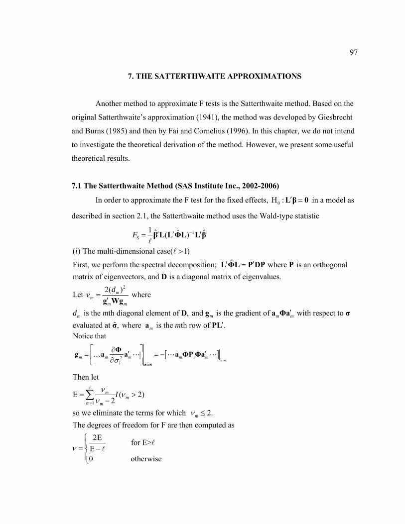
97

7. THE SATTERTHWAITE APPROXIMATIONS

Another method to approximate F tests is the Satterthwaite method. Based on the

original Satterthwaite’s approximation (1941), the method was developed by Giesbrecht

and Burns (1985) and then by Fai and Cornelius (1996). In this chapter, we do not intend

to investigate the theoretical derivation of the method. However, we present some useful

theoretical results.

7.1 The Satterthwaite Method (SAS Institute Inc., 2002-2006)


described in section 2.1, the Satterthwaite method uses the Wald-type statistic

0H : ′ =L β 0

1S

1 ˆ ˆˆ ( )

( ) The multi-dimensional case( 1)ˆFirst, we perform the spectral decomposition; where is an orthogonal

matrix of eigenvectors, and i

F

i

−′ ′ ′=

>

′ ′=

β L L ΦL L β

L ΦL Ρ DΡ ΡD

2

s a diagonal matrix of eigenvalues.2( )Let where

is the th diagonal element of , and is the gradient of with respect to ˆevaluated at , where is the th row of .

mm

m m

m m m

m

d

d mm

ν =′

′

′

g WgD g a Φa σ

σ a ΡLm

[ ]ˆ2

ˆ

Notice that

m m m m i miσ =

=

⎡ ⎤∂ ′ ′= = −⎢ ⎥∂⎣ ⎦ σ σσ σ

Φg a a a ΦΡ Φa…

1

Then let

E ( 2)2

so we eliminate the terms for which 2.The degrees of freedom for F are then computed as

2E for E> E

0 otherwise

mm

m m

m

Iν νν

ν

ν

=

= >−

≤

⎧⎪= −⎨⎪⎩

∑

98

2

S

( ) The one-dimensional case ( 1)In this case, statistic is simplified as

ˆ( ) . ˆNotice that we may use the t-statistic instead since th

iiF

F

=

′=

′L β

L ΦL

2

e numerator degrees of freedom equalsone. The denominator degrees of freedom is computed as

ˆ2( ) ,

ˆwhere is the gradient of with respec

ν′

=′

′

L ΦLg Wg

g L ΦL t to . (we assume that is estimable).′σ L β

7.2 The K-R, Satterthwaite, and Proposed Methods

In this section, we provide some useful lemmas that show the relationship among

the Satterthwaite, K-R and the proposed methods.

Lemma 7.2.1 When the Satterthwaite, the K-R and the proposed methods give 1,=

the same estimate of the denominator degrees of freedom.

Proof The K-R and the proposed methods give the same estimate of the denominator

degrees of freedom which is 1

2A

(corollary 5.3.5).

11 1

1 1

21 1

2 2

1

1 1

tr( )tr( ),

tr tr

( )

2 2( ) 2( )

r r

ij i ji j

r rji

iji j

r ri j

iji j

r r

ij i ji j

A w

w

w

A w

= =

= =

= =

= =

′= =

′

′′ ⎛ ⎞⎛ ⎞= ⎜ ⎟⎜ ⎟′ ′⎝ ⎠ ⎝ ⎠′ ′

=′

′ ′⇒ = =

′′ ′

∑∑

∑∑

∑∑

∑∑

LLΘΦΡ Φ ΘΦΡ Φ ΘL ΦL

LL ΦΡ ΦLL ΦΡ ΦL ΦL L ΦL

L ΦΡ ΦLL ΦΡ ΦLL ΦL

L ΦL L ΦLg WL ΦΡ ΦLL ΦΡ ΦL

1 where [ ]

By noticing that , the proof is completed.

i r

iiσ

×′=

∂= −

∂

g L ΦΡ ΦLg

Φ ΦΡ Φ

99

Note Even though the estimates of the denominator degrees of freedom are the same,

the true levels do not have to be the same for the Satterthwaite method and the K-R and

proposed methods. This is because the statistics used are not the same. The Satterthwaite

statistic uses as the estimator of the variance-covariance matrix of the fixed effects

estimator, whereas the K-R and the proposed methods statistic uses . The following

corollary clarifies this fact.

Φ

AΦ

Corollary 7.2.2 When , and 1= Aˆ ˆ ,=Φ Φ then the Satterthwaite, K-R and proposed

methods are identical.

Proof From lemma 7.2.1, the Satterthwaite, K-R and proposed methods give the same

estimate of the denominator degrees of freedom. Since the scale is 1 (corollary 5.3.5) and

then we have the same statistics for all approaches. This shows that the four

approaches are identical.

Aˆ ˆ ,=Φ Φ

Corollary 7.2.3 In balanced mixed classification models, and when , the

Satterthwaite, K-R and proposed methods are identical. The denominator degrees of

freedom and the scale estimate are

1=

2

2 and 1A

respectively.

Proof: Direct form corollaries 5.3.5, 6.1.1.2, and 7.2.2.

Lemma 7.2.4 SWhen 1, then the Satterthwaite statistic F= ≥ the K-R and the proposed

methods statistic for variance components models.F

Proof It suffices to show that Aˆ ˆ′ ′≥L Φ L L ΦL .

A1 1

A1 1

ˆˆ ˆ ˆ ˆ ˆ ˆ ˆˆSince 2 ( )

ˆˆ ˆ ˆ ˆ ˆ ˆ ˆˆ2 ( )

Notice that

r r

ij ij i ji j

r r

ij ij i ji j

w

w

= =

= =

⎧ ⎫= + −⎨ ⎬

⎩ ⎭⎧ ⎫

⇒ − = −⎨ ⎬⎩ ⎭

∑∑

∑∑

Φ Φ Φ Q Ρ ΦΡ Φ

Φ Φ Φ Q Ρ ΦΡ Φ

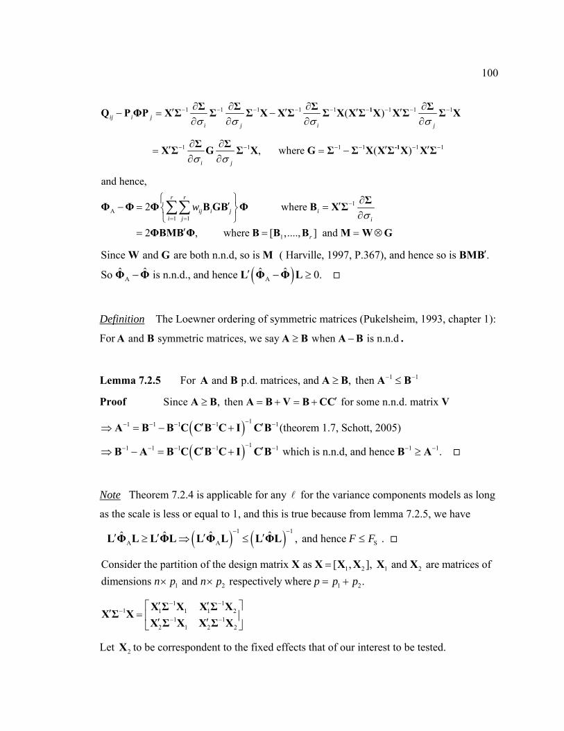
100

1 1 1 1 1 1 1( )ij i ji j i jσ σ σ σ

− − − − − − − − −∂ ∂ ∂ ∂′ ′ ′ ′− = −∂ ∂ ∂ ∂

1Σ Σ Σ ΣQ Ρ ΦΡ Χ Σ Σ Σ Χ Χ Σ Σ Χ Χ Σ Χ Χ Σ Σ Χ1

1 1 1 1 , where ( )i jσ σ

− − − − −∂ ∂ 1 1−′ ′ ′= = −∂ ∂

-1Σ ΣΧ Σ G Σ Χ G Σ Σ Χ Χ Σ Χ Χ Σ

1A

1 1

1

and hence,

2 where

2 , where [ ,...., ] and

r r

ij i j ii j i

r

wσ

−

= =

⎧ ⎫ ∂′ ′− = =⎨ ⎬ ∂⎩ ⎭′= =

∑∑ ΣΦ Φ Φ B GB Φ B ΧΣ

ΦBMB Φ B B B M W G= ⊗

( )A A

Since and are both n.n.d, so is ( Harville, 1997, P.367), and hence so is .ˆ ˆ ˆ ˆSo is n.n.d., and hence 0.

′

′− − ≥

W G M BMB

Φ Φ L Φ Φ L

Definition The Loewner ordering of symmetric matrices (Pukelsheim, 1993, chapter 1):

For . and symmetric matrices, we say when is n.n.d≥ −A B A B A B

Lemma 7.2.5 For 1 1 and p.d. matrices, and , then − −≥ ≤A B A B A B

Proof Since , then for some n.n.d. matrix ′≥ = + = +A B A B V B CC V

( )( )

11 1 1 1 1

11 1 1 1 1 1 1

(theorem 1.7, Schott, 2005)

which is n.n.d, and hence .

−− − − − −

−− − − − − − −

′ ′⇒ = − +

′ ′⇒ − = + ≥

A B B C C B C Ι C B

B A B C C B C Ι C B B A

Note Theorem 7.2.4 is applicable for any for the variance components models as long

as the scale is less or equal to 1, and this is true because from lemma 7.2.5, we have

( ) ( )1 1

A Aˆ ˆ ˆ ˆ , and hence .F F

− −′ ′ ′ ′≥ ⇒ ≤ ≤L Φ L L ΦL L Φ L L ΦL S

1 2 1 2

1 2 1 2

Consider the partition of the design matrix as [ , ], and are matrices of dimensions and respectively where . n p n p p p p

=× × = +

Χ Χ Χ Χ Χ Χ

1 11 1 1 1 2

1 12 1 2 2

− −−

− −

′ ′⎡ ⎤′ = ⎢ ⎥′ ′⎣ ⎦

Χ Σ Χ Χ Σ ΧΧ Σ Χ

Χ Σ Χ Χ Σ Χ

Let to be correspondent to the fixed effects that of our interest to be tested. 2Χ

101

Consider the case where 1

1 2(a) . −′ =Χ Σ Χ 0 1

2 2(b) ( ) where is a fixed matrix. is invertible when is a full column rankmatrix.

f−′ =Χ Σ Χ σ A A A Χ

Lemma 7.2.6 For a model that satisfies conditions (a) and (b) mentioned above, we

have . 1 2A A=

Proof 112

2

According to above, where ( )f− ⎡ ⎤′ = =⎢ ⎥

⎣ ⎦

C 0ΧΣ Χ C σ A

0 C

[ ]

1 2

1

1 22

11 1

12

111

212

1 1 12 1 1

2

11

( )

Also, since , then

,

( ) ( ) ,( )

p p

pp p

p

−−

−

× ×

−−

−

×− − −× − −×

×

−

⎡ ⎤′⇒ = = ⎢ ⎥

⎣ ⎦⎡ ⎤′ ′= ⎣ ⎦⎡ ⎤ ⎡ ⎤′ ′ ′= =⎢ ⎥ ⎢ ⎥

⎣ ⎦⎣ ⎦⎡ ⎤ ⎡ ⎤⎡ ⎤′ ′ ′ ′= = =⎢ ⎥ ⎢ ⎥⎣ ⎦ ′ ′⎢ ⎥ ⎣ ⎦⎣ ⎦

=

-1 C 0Φ ΧΣ Χ

0 C

L 0 B

0C 0L ΦL 0 B B C B

B0 C

0 0 0Θ L L ΦL L B C B 0 B

0 B B C B BB

C 0ΦΘΦ

0

11

1 1 1 1 1 11 12 22 2( ) ( )

−

− − − − − −− −

⎡ ⎤ ⎡ ⎤⎡ ⎤ ⎡=⎢ ⎥ ⎢ ⎥⎢ ⎥ ⎢′ ′ ′ ′⎣ ⎦ ⎣⎣ ⎦ ⎣ ⎦

0 0 0 0C 00 B B C B B 0 C B B C B B CC 0 C 2 2

⎤⎥⎦

11

2

1

1 1 1 1 21 1 1 12 2 22 2 2 2

Moreover, since then

( )( )

ii

i

i

ii

ii

σσ

σ

σ

σσ

−

− − − −− − − −

∂⎡ ⎤⎢ ⎥∂∂ ⎢ ⎥′= =

∂⎢ ⎥∂⎢ ⎥∂⎣ ⎦

∂⎡ ⎤⎡ ⎤⎢ ⎥∂⎡ ⎤ ⎢ ⎥⎢ ⎥= = ∂⎢ ⎥ ⎢ ⎥′ ′′ ′ ∂⎢ ⎥⎣ ⎦ ∂⎢ ⎥⎣ ⎦⎢ ⎥∂⎣ ⎦

C 0ΣΡ Χ Χ

C0

C 0 0 00 0

ΦΘΦΡ C0 C B B C B B C0 C B B C B B C C0

1 1 1 1 22 2 2So, tr( ) tr ( ) (7.1)i

iσ− − − −⎛ ⎞∂′ ′= ⎜ ⎟∂⎝ ⎠

CΘΦΡΦ C B B C B B C

11 2

2 2( ) 1 ( )Since ( ) , then

( ) ( )i i

f fff fσ σ

−− ∂ ∂ ∂

= = =∂ ∂ ∂C A σ σC σ A C A Ι

σ σ iσ

102

So, expression (7.1) above can be simplified as

( )1 1 12 2

1 ( ) tr( ) tr ( )( )i

i

ff σ

− − −∂ ′ ′=∂σΘΦΡ Φ C B B C B B

σ

( )1 1 12 2

1 ( ) ( ) tr ( ) (7.2)( ) ( )i i

f ff fσ σ

− − −∂ ∂′ ′= =∂ ∂σ σB C B B C B

σ σ2

2

( ) ( ) tr( )tr( ) (7.3)[ ( )]i j

i j

f ff σ σ

∂ ∂⇒ =

∂ ∂σ σΘΦΡ Φ ΘΦΡ Φ

σ

1 1 1 11 1 1 1 222 2 22 2 2

1 1 1 1 1 1 1 12 22 2 2 2 2 2

Also,

( )( )

( ) ( )

So,

i j

ji

i j

σσ

σ σ

− − − −− − − −

− − − − − − − −

⎡ ⎤⎡ ⎤⎢ ⎥⎢ ⎥ ∂= ∂ ⎢ ⎥⎢ ⎥ ′ ′′ ′

∂⎢ ⎥∂⎢ ⎥⎣ ⎦ ⎣ ⎦⎡ ⎤⎢ ⎥∂ ∂= ⎢ ⎥′ ′ ′ ′

∂ ∂⎢ ⎥⎣ ⎦

0 00 0CΦΘΦΡ ΦΘΦΡ C 0 C B B C B B C0 C B B C B B C

0 0C C0 C B B C B B C C B B C B B C

( )

1 1 1 1 1 1 1 12 22 2 2 2 2 2

1 1 1 1 1 12 2 2 22

tr( ) tr ( ) ( )

1 ( ) ( ) tr ( ) ( )[ ( )]

i ji j

i j

f ff

σ σ

σ σ

− − − − − − − −

− − − − − −

⎛ ⎞∂ ∂′ ′ ′ ′= ⎜ ⎟⎜ ⎟∂ ∂⎝ ⎠∂ ∂ ′ ′ ′ ′=∂ ∂

C CΘΦΡ ΦΘΦΡ Φ C B B C B B C C B B C B B C

σ σ C B B C B B C B B C B Bσ

( )1 1 1 1 1 12 2 2 22

2

1 ( ) ( ) tr ( ) ( ) [ ( )]

( ) ( ) (7.4[ ( )]

i j

i j

f ff

f ff

σ σ

σ σ

− − − − − −∂ ∂ ′ ′ ′ ′=∂ ∂

∂ ∂=

∂ ∂

σ σ B C B B C B B C B B C Bσ

σ σσ

)

1 2

From expressions 7.3 and 7.4, we have tr( )tr( ) tr( ),

and hence i j i j

A A

=

=

ΘΦΡ Φ ΘΦΡ Φ ΘΦΡ ΦΘΦΡ Φ

Lemma 7.2.7 For a model that satisfies conditions (a) and (b) mentioned above

The K-R and the proposed approaches are identical. ( )i

The Satterthwaite, K-R and proposed approaches give the same estimate

of the denominator degrees of freedom given that the estimate > 2.

( )ii

103

If , and the estimate of the denominator degrees of freedom >2, ( )iii Aˆ =Φ Φ

2

then the Satterthwaite, K-R and proposed methods are identical.

Proof Observe that ( )i 1A A= (lemma 7.2.6), and hence the K-R, and the proposed

methods are identical (corollary 5.3.3). They all give 1 and 2

2A

as the estimates of the

scale and the denominator degrees of freedom respectively (theorems 5.3.1 and 5.3.2).

( )ii Claim 2

2

2 2 for any .A

m

m m

d m=′g Wg

Proof 1 11 1

tr( )tr( ) where [tr( )] ,r r

ij i j i ri j

A w ×= =

′= = =∑∑ ΘΦΡΦ ΘΦΡ Φ a Wa a ΘΦΡΦ

1

( ) ( )Since form expression (7.2), tr( ) , then ( ) ( )i

i i r

f ff fσ σ

×

⎡ ⎤∂ ∂= = ⎢ ⎥∂ ∂⎣ ⎦

σ σΘΦΡ Φ aσ σ

2 2 2

2 1 1

And hence

2 2 2 2[ ( )] ( )the R.H.S where .A A i r

f fσ

×

⎡ ⎤∂= = = = = ⎢ ⎥′ ′ ∂⎣ ⎦

σ σga Wa g Wg

1 1

111 22

21 1

Since where is the th row of , then

where is the th row of .

1 ( )[ ( )]

m m m m m m mi ir r

m

mm m m m m

i ir r

m

m

ff

σ σ

σ σ

× ×

−−−

× ×

⎡ ⎤ ⎡ ⎤∂ ∂′ ′= =⎢ ⎥ ⎢ ⎥∂ ∂⎣ ⎦ ⎣ ⎦

⎡ ⎤ ⎡ ⎤ ′ ′∂ − ∂′ ′ ′ ′⇒ = = = −⎢ ⎥ ⎢ ⎥∂ ∂⎣ ⎦ ⎣ ⎦

Φ Φg a a a ΡL g b L Lb

b Ρ

b B C BC σg b B Bb b B A Bbσ

′ ′

122 2

12

1 1

( )( )

2 2 ( )And the L.H.S( ) ( )

m

i r

m m

m m m m

i ir r

ff

d d f

f f

σ

σ σ

×

−

× ×

⎡ ⎤∂⎢ ⎥∂⎣ ⎦

⎛ ⎞= = ⎜ ⎟′ ′ ′′ ⎝ ⎠⎡ ⎤ ⎡ ⎤∂ ∂

⎢ ⎥ ⎢ ⎥∂ ∂⎣ ⎦ ⎣ ⎦

b σσ

σg Wg b B C Bbσ σW

12

2 2

1 1

Notice that .

2 2[ ( )] the L.H.S the R.H.S( ) ( )

m m m m m

m

m m

i ir r

d

d f

f fσ σ

−

× ×

′ ′ ′ ′= =

⇒ = = =′ ′⎡ ⎤ ⎡ ⎤∂ ∂

⎢ ⎥ ⎢ ⎥∂ ∂⎣ ⎦ ⎣ ⎦

b B C Bb b L ΦLb

σg Wg σ σW

We note that the L.H.S does not depend on row , and this means that our claim is truefor any row .

mm

104

2

2

22 2

2 2Since >2 for any ,A

22E2 2then E 2 , and the L.H.S.E

mm

m m

mm m

m m m m m m

d m

dd d

ν

ν

= =′

⎛ ⎞= − = = =⎜ ⎟′ ′ ′−⎝ ⎠

g Wg

g Wg g Wg g Wg

( )iii Direct from parts ( ) and ( ).ii iii

Comments

( )i When conditions (a) and (b) are satisfied, then the K-R and the proposed methods are

identical. However, these conditions are not enough to make the Satterthwaite approach

identical with the K-R and the proposed methods.

( )ii However, when the denominator degrees of freedom estimate is greater than two,

conditions (a) and (b) are enough to make the Satterthwaite produce the same estimate of

the denominator degrees of freedom produced by the K-R and the proposed methods.

When the K-R and the proposed methods’ estimate of the denominator degrees of

freedom is less or equal than two, the Satterthwaite estimate is zero.

( )iii

( )iv Even though the Satterthwaite method produces the same estimate of the

denominator degrees of freedom as the one produced by K-R and the proposed methods

when the denominator degrees of freedom estimate is greater than two and conditions (a)

and (b) are satisfied, we should notice that this does not mean that the Satterthwaite

approach is identical to the K-R and proposed methods. This is true because the statistics

used are different. The Satterthwaite statistic uses as an estimator of the variance-

covariance matrix of the fixed effects estimator, whereas the K-R and the proposed

methods statistic uses .

Φ

AΦ

( )v Conditions (a) and (b) are not enough to make . For example, in BIB designs,

conditions (a) and (b) are satisfied; however, (chapter 8).

Aˆ ˆ=Φ Φ

Aˆ ˆ≠Φ Φ

105

8. SIMULATION STUDY FOR BLOCK DESIGNS

To compare the tests discussed in the previous chapters, we have conducted

simulation studies for three different types of block designs: partially balanced

incomplete block design (PBIB), balanced incomplete block design (BIB), and complete

block design with missing data (two observations to be missing: one is from the first

block under first treatment and the other one is from the second block under the second

treatment). To test the fixed effects in these models, there are two approaches. The first

approach is the intra-block approach where we consider the blocks fixed, so that only the

within blocks information is utilized. Even though this approach leads to exact F tests, it

does not lead to an optimal test. When the design is efficient and blocking is effective,

this approach is close to optimal. We use the second approach where the blocks are

considered random, and information from both within and between blocks is utilized.

With the second approach, the model does not satisfy Zyskind’s condition, so it is not a

Rady model, and hence we do not have an exact F-test to test the fixed effect.

8.1 Preparing Formulas for Computations

Model for a Block Design

ij i j ijy b eμ α= + + +

for 1,....., , 1,....., , i t j= = s where is the generalμ mean, iα is the treatments effects,

jb is the blocks effects, 2 2N(0, ), N(0, )j b ij eb eσ σ∼ ∼ , and are all

independent.

's and 'sjb eij

1 1

The model can be expressed as ,where [ , ] , [ , , ] ,

n

s tb bμα α

= + + +′ ′= =

y 1 Aa Bbb a

e

22 2 2

1 21

E( ) , and Var( ) where and n e n b i i ni

μ σ σ σ=

′ ′= + = = + = = =∑y 1 Aa y Σ Ι BB D D Ι D BB

Suppose that we are interested in testing: 1H: tα α= = ′⇔ =L β 0

106

[ ]1

0 1 1 0 00 0 1 1 0

where ,

0 0 0 1 1

tμ α α

−⎡ ⎤⎢ ⎥−⎢ ⎥′ ′= =⎢ ⎥⎢ ⎥−⎣ ⎦

L β

The design matrix; is not of full column rank. We can proceed with this

parameterization using the g-inverse. However, to simplify our computations, we will

reparameterize the model so will be a full column rank matrix.

[ , ]n=Χ 1 A

Χt

1 11

Reparameterize the model in the way that with 0.t ii

μ α α α∗ ∗ ∗ ∗ ∗−

=

′ ⎡ ⎤= =⎣ ⎦ ∑β

0 1 0 00 0 1 0

and ,

0 0 0 1

∗

⎡ ⎤⎢ ⎥⎢ ⎥′ =⎢ ⎥⎢ ⎥⎣ ⎦

L

To simplify our notation, from now on, consider , , and .∗ ∗ ∗= = =Χ Χ L L β β

The REML Estimates

2 22 2

1 1 1 1 1 1

The REML equations are:2 ( ) 2 ( )tr( ) , tr( ) ,

where ( ) ( ) .e bσ σ

− − − − − −

∂ ∂′ ′= − + = − +∂ ∂

′ ′ ′ ′= − =

σ σG y GGy GD y GD Gy

G Σ Σ Χ ΧΣ Χ Χ Σ Κ Κ ΣΚ Κ

( ) 1, 1

1

A useful form to find the REML estimates by iteration is

tr ,

where ( 1) ( ,...., ) (Searle ., 1992, chapter 6).

r ri j i ii j

rr et alσ σ==

′=

′× =

D GD G σ y GD Gy

σ

2

2 2

To estimate , we may use the inverse of the expected information matrix where,

1E tr( ) (Searle ., 1992, chapter 6)2

ij

j ii j

w

et alσ σ

⎡ ⎤∂− =⎢ ⎥

∂ ∂⎢ ⎥⎣ ⎦GD GD

2 22

2 22 2 2 2

1 1and hence E tr( ), E tr( ),( ) 2 ( ) 2e bσ σ

⎡ ⎤ ⎡ ⎤∂ ∂− = − =⎢ ⎥ ⎢ ⎥∂ ∂⎣ ⎦ ⎣ ⎦

G GD GD

107

and 2

22 2

1E tr( ) 2e bσ σ

⎡ ⎤∂− =⎢ ⎥∂ ∂⎣ ⎦

GD G

The entries of the inverse of the information matrix are estimated by using the REML

estimates of 2 2 and e bσ σ .

How we get matrix K

[ ] for any (Searle ., 1992, chapter 6)n et al′ ′ ′= − ΧΚ C Ι Ρ C

Notice that [ ] [ ] .However, it's desirable to have with a full row rank so is invertible.For our example, we obtain , and then we can pick the independent rows of it.

n

n

′ ′ ′= − = − =′ ′

−

Χ

Χ

Κ Χ C Ι Ρ Χ C Χ Χ 0Κ Κ ΣΚ

Ι Ρ

Computing , and iΡ ijQ ijR

11 1 1

1 2 2 ,e eσ σ

−− − − −∂ ∂′ ′ ′= = − = −

∂ ∂Σ ΣΡ Χ Χ ΧΣ Σ Χ ΧΣ Σ Χ1

11 1 1

2 22 2b bσ σ

−− − − −∂ ∂′ ′ ′= = − = −

∂ ∂Σ ΣΡ Χ Χ ΧΣ Σ Χ ΧΣ D Σ Χ1

1 11 1 1 1 1 1

11 2 2 2 2

1 11 1 1 1 1

12 21 22 2 2 2

,e e e e

e b e b

σ σ σ σ

σ σ σ σ

− −− − − − − −

− −− − − − − −

∂ ∂ ∂ ∂′ ′ ′= = =∂ ∂ ∂ ∂

∂ ∂ ∂ ∂′ ′ ′= = = =∂ ∂ ∂ ∂

Σ Σ Σ ΣQ Χ Σ Χ ΧΣ Σ Σ Χ ΧΣ Σ Σ Χ

Σ Σ Σ ΣQ Q Χ Σ Χ ΧΣ Σ Σ Χ ΧΣ Σ D Σ Χ1

1 11 1 1

22 2 22 2b bσ σ

− −− − −∂ ∂′ ′= =

∂ ∂Σ ΣQ Χ Σ Χ ΧΣ D Σ D Σ Χ .

, for all , 1, 2 (clear).ij i j= =R 0

The above quantities are to be estimated by using the REML estimates of . σ

Block designs with equal block sizes

2

2 2 1 1

When the design has equal block sizes (e.g., BIBD, and PBIBD), then

where is the block size. Also, , where . ,s k

s k k e k b k s kk σ σ − −

′= = ⊗

= ⊗ = + = ⊗

D BB Ι J

Σ Ι Σ Σ Ι J Σ Ι Σ

( )211 2 2

2 2 2

1where = (Schott, 2005, theorem 1.7)bk e k b k k k

e e bkσσ σ

σ σ σ−− ⎡ ⎤

= + −⎢ ⎥+⎣ ⎦Σ Ι J Ι J

108

11 1 1 1 2

2 22 2 2( )b b e kσ σ σ

−− − − − ′∂ ∂′ ′ ′= = − = − = −

∂ ∂ +ΧD ΧΣ ΣΡ Χ Χ ΧΣ Σ Χ ΧΣ D Σ Χ 2 2

bσ

1 1 1 22 2 2 2 2Notice that ( )( ) .

( ) ( )s k

s k s k s k ke b e bk kσ σ σ σ

− − − ⊗= ⊗ ⊗ = ⊗ = =

+ +Ι J DD Σ Ι J Ι Σ Ι J Σ

1 11 1

12 21 2 2 2 2

1 1 1 22 2 2 3

( )

e b e b

e bk

σ σ σ σ

σ σ

− −− − −

− − −

∂ ∂ ∂ ∂′ ′= = =∂ ∂ ∂ ∂

′′= =

+

Σ Σ Σ ΣQ Q Χ Σ Χ ΧΣ Σ Σ

ΧD ΧΧΣ Σ D Σ Χ

1Χ

1 11 1 1 2 2 2

22 2 2 122 2 2 2 3 2 2 3( ) ( )b b e b e b

k kk kσ σ σ σ σ σ

− −− − − ′ ′∂ ∂′ ′= = = =

∂ ∂ + +ΧD D Χ ΧD ΧΣ ΣQ Χ Σ Χ ΧΣ D Σ D Σ Χ Q= .

Lemma For the mixed linear model , and the

null hypothesis is .

1

, N( , ), r

i ii

σ=

= + =∑y Χβ u u 0 Σ Σ V∼

0H : ′ =L β 0

( )i In simulation of the K-R and Satterthwaite statistics ( ) under , it suffices

to take the fixed effects, .

KR Sand F F

>

0H

=β 0

( )ii KR KR S S( ) ( ) and ( ) ( ) for any constant 0.F F a F F a a= =u u u u

Proof 1KR A

1 ˆ ˆˆ( ) ( ) ( ) ( )i F −′ ′ ′ ′= L β L Φ L L β .

KR 0

A

1

To simulate under H , we generate N( , ), and then where .ˆ ˆ ˆHowever, we should notice that , , and do not depend on . Indeed, they depend

only on .ˆ ˆ ˆ ˆ ˆMoreover,

F

−

′= + =

′ ′= =

u 0 Σ y Χβ u L β 0

Σ Φ Φ Χβu

β ΦΧΣ y ΦΧΣ

∼

1 1

1 10 0 0

S 0

ˆ ˆ( ) .ˆ ˆ ˆˆ ˆ ˆ ˆ (under H ) where is calculated from with .

Similarly, it can be shown that in simulation of under H , it suffices to take F

− −

− −

′+ = +

′ ′ ′ ′ ′ ′ ′⇒ = + = =

= ==

Χβ u β ΦΧΣ u

L β L β L ΦΧΣ u L ΦΧΣ u L β β βu y β 0

β 0

ˆ

( ) ( )2 2

1 11 2 1 2

1 1

ˆ ˆ( ) Observe that N( , ) N( , ), and hence ( ) ( ).

ˆ ˆ ˆ ˆ( ) ( ) ( ) ( ),

ˆ ˆˆ ˆ ˆ ˆ( ) ( ) ( ) ( ) ( ) ( ).

ii a a a a

a a a a

a a a a a a

− −− −

− −

⇔ =

′ ′= = =

′ ′= = =

u 0 Σ u 0 Σ Σ u Σ u

Φ u ΧΣ u Χ ΧΣ u Χ Φ u

β u Φ u ΧΣ u u Φ u ΧΣ u u β u

∼ ∼

109

1 1 14 4

1 1 1

ˆ ˆ( ) 1 ( ) 11ˆ ˆ ˆ ˆ ˆ( ) ( ) ( ) ( ) ( ) ( )

ˆ ˆ( ) ( )ˆ ˆ ˆand ( ) ( ) ( ) ( )

i ii i

iji j

aa a aa a

a aa a a a

σ σ

σ σ

− − −

− − −

∂ ∂−′ ′= − = − =∂ ∂

∂ ∂′=∂ ∂

Σ u Σ uΡ u ΧΣ u Σ u Χ ΧΣ u Σ u Χ Ρ u

Σ u Σ uQ u ΧΣ u Σ u Σ u Χ

,

1 1 16 6

ˆ ˆ1 ( ) ( ) 1ˆ ˆ ˆ ( ) ( ) ( ) ( ).iji ja aσ σ

− − −∂ ∂′= =∂ ∂Σ u Σ uΧΣ u Σ u Σ u Χ Q u

( )( )

11 1 1 1

11 1 1 12 2

ˆ ˆ ˆ ˆAlso, since ( ) ( ) ( ) ( ) ( )

1 1ˆ ˆ ˆ ˆ ( ) ( ) ( ) ( ) ( ),

a a a a a

a a

−− − − −

−− − − −

′ ′= −

⎡ ⎤′ ′= − =⎢ ⎥⎣ ⎦

G u Σ u Σ u ΧΣ u Χ ΧΣ u

Σ u Σ u ΧΣ u Χ ΧΣ u G u

1

, 1

1

44

, 1

ˆ ˆ( ) ( )then ( ) 2 tr ( ) ( ) (section 6.1.2)

ˆ ˆ1 ( ) ( ) 2 tr ( ) ( ) ( ).

Since

r

i j i jm

r

i j i jm

a aa a a

aa

σ σ

σ σ

−

=

−

=

⎡ ⎤⎧ ⎫⎛ ⎞∂ ∂⎪ ⎪⎢ ⎥≈ ⎜ ⎟⎨ ⎬⎜ ⎟⎢ ⎥∂ ∂⎪ ⎪⎝ ⎠⎩ ⎭⎣ ⎦

⎡ ⎤⎧ ⎫⎛ ⎞∂ ∂⎪ ⎪⎢ ⎥= =⎜ ⎟⎨ ⎬⎜ ⎟⎢ ⎥∂ ∂⎪ ⎪⎝ ⎠⎩ ⎭⎣ ⎦

Σ u Σ uW u G u G u

Σ u Σ uG u G u W u

R 2A A KR KR

S S

ˆ ˆ, then we obtain ( ) ( ), and hence hence ( ) ( )

and ( ) ( ). ij a a F F a

F F a

= =

=

0 Φ u Φ u u

u u

= u

e

8.2 Simulation Results

Seven approaches for testing fixed effects are considered in the simulation study:

Kenward-Roger (after modification), Kenward-Roger before the modification, Kenward-

Roger using the conventional variance-covariance of the fixed effects, Satterthwaite,

Containment, and our proposed methods. Five settings for the ratio of and bσ σ that are

denoted by ρ have been used: 0.25, 0.5, 1, 2, 4. For each setting of ρ , 10,000 data sets

have been simulated from the corresponding multivariate distribution with zero treatment

effects. The level for each test, mean of scales, and mean of the denominator degrees of

freedom were computed for the data sets at nominal 0.05. We use to denote levels

below 0.0400 or above 0.0600, and† for levels between 0.0400 and 0.0449 or between

††

0.0551 and 0.0600. So, all unmarked levels are between 0.0450 and 0.0550. For each data

110

set the REML estimates of the variance components have been calculated by the iteration

method mentioned above, and convergence was achieved for almost all data sets. The

convergence rate is reported. Also, we present the percentage relative bias in the

conventional and the adjusted estimator of variance-covariance matrix of the fixed effects

estimator. In each type of block design, we consider some examples where we have

different efficiency factors. The relative efficiency of a random block model to a

complete block model for a given number t of treatments and a given number of n of

observations can be expressed as

( )2

111

/ where , , and .trace ( 1)

n t tt nE

tρ

ρ

ρ −−−′ ′ ′= = + = =

⎡ ⎤′ ′ −⎢ ⎥⎣ ⎦

BB Ι Τ Τ Ι Τ 1 0Τ A Σ A Τ

Σ

The efficiency factor which is denoted by is defined to be the lower bound of , and itdescribes the design alone. For an equireplicate block design with equal block sizes,

q E

( )( )1 where is the replication of the treatments (Birkes, 2006).

trace

Observe that BIB and PBIB designs are equireplicate and have equal block sizes.

tq rr

+

−=

′ −⎡ ⎤⎣ ⎦BA Ι Ρ A

8.2.1 Partially Balanced Incomplete Block Design (PBIB)

I. The first PBIB design (PBIB1) is from Cochran and Cox (1957, P.456) where we have

fifteen blocks, fifteen treatments, four treatments per block and 0.7955q = .

Table 1.1 PBIB1 ( 15, 4, and 6t s k n 0)= = = =

Block Treat. Block Treat. Block Treat. 1 15,9,1,13 6 12,4,3,1 11 9,7,10,3 2 5,7,8,1 7 12,14,15,8 12 8,6,2,9 3 10,1,14,2 8 6,3,14,5 13 5,9,11,12 4 15,11,2,3 9 5,4,2,13 14 7,13,14,11 5 6,15,4,7 10 10,12,13,6 15 10,4,8,11

111

Table 1.2 Simulated size of nominal 5% Wald F- tests for PBIB1

ρ K-R∗ K-R∗∗ K-R Prop.1 Prop.2 Satter Contain 0.25 0.0528 ††0.0390 0.0466 0.0478 0.0468 ††0.0697 ††0.06740.5 0.0536 †0.0423 0.0475 0.0483 0.0480 ††0.0622 †0.0558 1.0 †0.0573 0.0486 0.0521 0.0521 0.0521 †0.0560 0.0528 2.0 0.0548 0.0467 0.0480 0.0480 0.0480 0.0497 0.0483 4.0 0.0544 0.0481 0.0484 0.0484 0.0484 0.0492 0.0485

A

ˆ ˆ before modification, with using instead of . S.E. of entries (0.0019,0.0025)∗ ∗ ∗ ∈Φ Φ

Table1.3 Mean of estimated denominator degrees of freedom for PBIB1

ρ K-R∗ K-R∗∗ K-R Prop.1 Prop.2 Satter Contain 0.25 48.8821 31.9638 39.3355 41.7298 40.2042 38.8929 31 0.5 47.4572 31.8812 38.4884 39.6942 38.9313 38.3272 31 1.0 43.1678 30.0484 34.6682 34.8640 34.7480 34.6475 31 2.0 40.5233 29.9220 32.1060 32.1205 32.1125 32.1052 31 4.0 39.7016 30.5696 31.2880 31.2889 31.2884 31.2830 31

A

ˆ ˆ before modification, with using instead of . ∗ ∗ ∗ Φ Φ

Table 1.4 Mean of estimated scale for PBIB1

ρ K-R∗ K-R∗∗ K-R Prop.1 Prop.2 0.25 0.9890 0.8787 0.9974 0.9954 0.9975 0.5 0.9916 0.9459 0.9991 0.9978 0.9989 1.0 0.9913 0.9829 0.9999 0.9996 0.9998 2.0 0.9902 0.9970 1.0000 1.0000 1.0000 4.0 0.9898 0.9996 1.0000 1.0000 1.0000

A


Table 1.5 Percentage relative bias in the variance estimates,

convergence rate (CR) and efficiency ( E ) for PBIB1 ρ Φ AΦ CR E

0.25 -6.5 1.6 0.9993 0.9604 0.5 -4.2 1.0 0.9999 0.8999 1.0 -0.6 1.5 1.0000 0.8378 2.0 -0.4 0.0 1.0000 0.8080 4.0 -0.6 -0.5 1.0000 0.7987

112

II. The second design (PBIB2) is from Green (1974, P.65) where we have forty-eight

blocks, sixteen treatments, two treatments per block and 0.4762q = .

Table 1.6 PBIB2 design ( 16, 48, 2,and 96)t s k n= = = =

blk trt blk trt blk trt blk trt blk trt blk trt 1 1,2 9 5,8 17 10,12 25 1,5 33 2,14 41 7,15 2 1,3 10 6,7 18 11,12 26 1,9 34 6,10 42 11,153 1,4 11 6,8 19 13,14 27 1,13 35 6,14 43 4,8 4 2,3 12 7,8 20 13,15 28 5,9 36 10,14 44 4,12 5 2,4 13 9,10 21 13,16 29 5,13 37 3,7 45 4,16 6 3,4 14 9,11 22 14,15 30 9,13 38 3,11 46 8,12 7 5,6 15 9,12 23 14,16 31 2,6 39 3,15 47 8,16 8 5,7 16 10,11 24 15,16 32 2,10 40 7,11 48 12,16

Table 1.7 Simulated size of nominal 5% Wald F- tests for PBIB2

ρ K-R∗ K-R∗∗ K-R Prop.1 Prop.2 Satter Contain 0.25 †0.0593 0.0532 †0.0568 †0.0585 †0.0573 ††0.0730 †0.0440 0.5 †0.0585 0.0529 †0.0561 †0.0579 †0.0565 ††0.0711 0.0453 1.0 †0.0570 0.0504 0.0540 0.0549 0.0543 ††0.0644 0.0468 2.0 †0.0557 0.0473 0.0508 0.0511 0.0509 0.0542 0.0480 4.0 †0.0562 0.0470 0.0493 0.0494 0.0493 0.0507 0.0480

A

ˆ ˆ before modification, with using instead of . S.E. of entries (0.0021,0.0026)∗ ∗ ∗ ∈Φ Φ

Table1.8 Mean of estimated denominator degrees of freedom for PBIB2

ρ K-R∗ K-R∗∗ K-R Prop.1 Prop.2 Satter Contain 0.25 83.6874 65.3837 72.6495 82.2865 74.7209 68.9973 33 0.5 79.8284 61.8836 69.0306 77.4455 70.9267 65.9502 33 1.0 65.6409 49.2069 55.8740 59.9145 56.9966 54.6475 33 2.0 49.9531 36.2898 41.2927 41.9262 41.5348 41.1791 33 4.0 43.6954 32.8601 35.2892 35.3400 35.3120 35.2835 33

A


113

Table 1.9 Mean of estimated scales for PBIB2

ρ K-R∗ K-R∗∗ K-R Prop.1 Prop.2 0.25 0.9953 0.9482 0.9981 0.9949 0.9973 0.5 0.9952 0.9511 0.9983 0.9952 0.9975 1.0 0.9948 0.9639 0.9991 0.9968 0.9984 2.0 0.9934 0.9859 0.9999 0.9991 0.9996 4.0 0.9917 0.9974 1.0000 0.9999 1.0000

Aˆ ˆ before modification, with using instead of . ∗ ∗ ∗ Φ Φ

Table 1.10

Percentage relative bias in the variance estimates, convergence rate (CR) and efficiency ( E ) for PBIB2

ρ Φ AΦ CR E

0.25 -7.0 -2.5 1.0000 0.9478 0.5 -7.0 -2.7 1.0000 0.8408 1.0 -5.9 -2.4 1.0000 0.6705 2.0 -3.3 -1.6 1.0000 0.5451 4.0 -2.6 -2.2 1.0000 0.4955

8.2.2 Balanced Incomplete Block Design (BIBD)

Since the design is balanced with respect to treatments, then it can be shown that

the model satisfies conditions (a) and (b) for theorem lemma 7.2.6, and hence 1 2A A= .

The K-R and the proposed approaches are identical. The scale estimate is 1 and the

denominator degree of freedom is estimate is 2

2A

(theorems 5.3.1 and 5.3.2, and corollary

5.3.3). The Satterthwaite method gives the same estimate of the denominator degrees of

freedom as the K-R and the proposed approaches when the estimate >2 (lemma 7.2.7).

Six BIB designs with different efficiency factors are adopted from Cochran and Cox

(1957, chapter 11). Notice that the efficiency factor simplified 1 1as 1 1

t kqrk tα −

= =−

where

is the replication of the treatments and is the number of blocks in which each pair oftreatments occur together (Kuehl, 2000, chapter 9).r α

114

I. In the first design (BIB1), where we have fifteen blocks, six treatments, and two treatments per block ( , and the efficiency factor, 6, 15, 2, and 30)t s k n= = = = 0.6q =

Table 2.1

BIB1 ( 6, 15, 2, and 30)t s k n= = = = Block Treat. Block Treat. Block Treat. Block Treat. Block Treat. 1 1,2 4 1,3 7 1,4 10 1,5 13 1,6 2 3,4 5 2,5 8 2,6 11 2,4 14 2,3 3 5,6 6 4,6 9 3, 5 12 3,6 15 4,5

Table 2.2 Simulated size of nominal 5% Wald F- tests for BIB1

ρ K-R∗ K-R&prop. Satter Contain 0.25 ††0.0786 ††0.0676 ††0.0998 ††0.0619 0.5 ††0.0731 ††0.0635 ††0.0930 †0.0589 1.0 ††0.0710 †0.0566 ††0.0746 0.0534 2.0 ††0.0697 †0.0551 †0.0599 0.0539 4.0 ††0.0727 0.0542 †0.0559 0.0540

before modification. S.E. of entries (0.0023,0.003)∗ ∈

Table 2.3 Mean of estimated denominator degrees of freedom for BIB1

ρ K-R∗ K-R&prop. Satter Contain 0.25 29.0917 20.1712 20.1712 10 0.5 28.0031 19.0591 19.0591 10 1.0 24.6097 15.5784 15.5784 10 2.0 21.0182 11.8539 11.8539 10 4.0 19.7201 10.4807 10.4807 10

before modification.∗

Table 2.4

Mean of estimated scales for BIB1 ρ K-R∗ K-R 0.25 0.9753 1.0000 0.5 0.9725 1.0000 1.0 0.9619 1.0000 2.0 0.9446 1.0000 4.0 0.9344 1.0000

before modification. ∗

115


convergence rate (CR) and efficiency ( E ) for BIB1 ρ Φ AΦ CR E

0.25 -16.0 -3.7 0.9968 0.9556 0.5 -13.5 -2.3 0.9978 0.8667 1.0 -8.9 -1.2 0.9994 0.7333 2.0 -2.0 -0.6 1.0000 0.6444 4.0 0.6 0.9 1.0000 0.6121

II. In the second design (BIB2), we have ten blocks, six treatments, and three treatments

per block ( , 6, 10, 3, and 30)t s k n= = = = 0.8q =

Table 2.6 BIB2 ( 6, 10, 3, and 30)t s k n= = = =

Block Treat. Block Treat.1 1,2,5 6 2,3,4 2 1,2,6 7 2,3,5 3 1,3,4 8 2,4,6 4 1,3,6 9 3,5,6 5 1,4,5 10 4,5,6

Table 2.7 Simulated size of nominal 5% Wald F- tests for BIB2 ρ K-R∗ K-R&prop. Satter Contain

0.25 ††0.0673 †0.0577 ††0.0830 ††0.0710 0.5 ††0.0670 †0.0584 ††0.0775 ††0.0664 1.0 ††0.0633 0.0524 ††0.0604 †0.0552 2.0 ††0.0606 0.0491 0.0515 0.0497 4.0 †0.0579 0.0474 0.0482 0.0475


116

Table 2.8

Mean of estimated denominator degrees of freedom for BIB2 ρ K-R∗ K-R&prop. Satter Contain

0.25 29.4561 20.5425 20.5425 15 0.5 28.5419 19.6163 19.6163 15 1.0 26.3744 17.4069 17.4069 15 2.0 24.7693 15.7620 15.7620 15 4.0 24.2247 15.2012 15.2012 15


Table 2.9 Mean of estimated scales for BIB2

ρ K-R∗ K-R 0.25 0.9761 1.0000 0.5 0.9749 1.0000 1.0 0.9701 1.0000 2.0 0.9653 1.0000 4.0 0.9632 1.0000



convergence rate (CR) and efficiency for BIB2 ρ Φ AΦ CR E

0.25 -12.0 -2.1 0.9977 0.9684 0.5 -7.4 0.2 0.9991 0.9143 1.0 -5.3 -2.1 1.0000 0.8500 2.0 -2.6 -2.0 1.0000 0.8154 4.0 -0.5 - 0.5 1.0000 0.8041

III. In the third design (BIB3), we have ten blocks, six treatments, and three treatments per block ( , 7, 7, 4, and 28)t s k n= = = = 0.8750q =

117


Block Treat. 1 3,5,6,72 1,4,6,73 1,2,5,74 1,2,3,65 2,3,4,76 1,3,4,57 2,4,5,6

Table 2.12 Simulated size of nominal 5% Wald F- tests for BIB3 ρ K-R∗ K-R&prop. Satter Contain 0.25 †0.0569 0.0472 ††0.0697 ††0.0769 0.5 ††0.0613 0.0508 ††0.0660 ††0.0644 1.0 ††0.0607 0.0494 †0.0553 0.0524 2.0 †0.0581 0.0450 0.0470 0.0454 4.0 †0.0570 0.0455 0.0456 0.0456







ρ K-R∗ K-R 0.25 0.9549 1.0000 0.5 0.9653 1.0000 1.0 0.9667 1.0000 2.0 0.9643 1.0000 4.0 0.9632 1.0000

118


convergence rate (CR) and efficiency for BIB3 ρ Φ AΦ CR E

0.25 -10.8 3.9 1.0000 0.9750 0.5 -8.9 -0.5 1.0000 0.9357 1.0 -0.4 2.2 1.0000 0.9000 2.0 -1.3 -0.9 1.0000 0.8824 4.0 -2.0 -1.9 1.0000 0.8769

IV. In the fourth design (BIB4), we have thirty six blocks, nine treatments, and two treatments per block ( , and 9, 36, 2, and 72)t s k n= = = = 0.5625q =

Table 2.16

BIB4 ( 9, 36, 2, and 72)t s k n= = = = Block Treat. Block Treat. Block Treat. Block Treat.

1 1,2 10 1,3 19 1,4 28 1,5 2 2,8 11 2,5 20 2,6 29 2,4 3 3,4 12 3,6 21 2,3 30 3,8 4 4,7 13 4,9 22 4,5 31 4,6 5 5,6 14 5,8 23 5,7 32 3,5 6 1,6 15 6,7 24 6,8 33 6,9 7 3,7 16 1,7 25 7,9 34 2,7 8 8,9 17 4,8 26 1,8 35 7,8 9 5,9 18 2,9 27 3,9 36 1,9


0.25 †0.0578 †0.0566 ††0.0731 0.0520 0.5 †0.0587 †0.0562 ††0.0709 0.0521 1.0 †0.0555 0.0524 ††0.0617 0.0501 2.0 †0.0598 0.0536 †0.0592 0.0525 4.0 †0.0599 0.0547 †0.0557 0.0546


119

Table 2.18


0.25 66.8712 58.3711 58.3711 28 0.5 63.3018 54.7945 54.7945 28 1.0 52.5089 43.9746 43.9746 28 2.0 41.8840 33.3083 33.3083 28 4.0 38.0104 29.4118 29.4118 28



ρ K-R∗ K-R 0.25 0.9966 1.0000 0.5 0.9961 1.0000 1.0 0.9942 1.0000 2.0 0.9906 1.0000 4.0 0.9883 1.0000




0.25 -7.5 -2.0 1.0000 0.9514 0.5 -5.9 -0.8 1.0000 0.8542 1.0 -4.2 -0.7 1.0000 0.7083 2.0 -0.7 0.5 1.0000 0.6111 4.0 0.9 1.1 1.0000 0.5758

V. In the fifth design (BIB5), we have ten blocks, six treatments, and three treatments per block , and ( 9, 18, 4, and 72)t s k n= = = = 0.8438q =

120

Table 2.21 BIB5 design ( 9, 18, 4, and 72)t s k n= = = =

Block Treat. Block Treat. Block Treat. 1 1,4,6,7 7 2,3,6,7 13 1,2,4,9 2 2,6,8,9 8 2,4,5,8 14 1,5,6,9 3 1,3,8,9 9 3,5,7,9 15 1,3,6,8 4 1,2,3,4 10 1,2,5,7 16 4,6,7,8 5 1,5,7,8 11 2,3,5,6 17 3,4,5,8 6 4,5,6,9 12 3,4,7,9 18 2,7,8,9

Table 2.22 Simulated size of nominal 5% Wald F- tests for BIB5 ρ K-R∗ K-R&prop. Satter Contain 0.25 0.0546 0.0532 ††0.0612 †0.0585 0.5 0.0534 0.0523 †0.0577 0.0546 1.0 0.0518 0.0494 0.0525 0.0514 2.0 0.0498 0.0468 0.0476 0.0480 4.0 0.0505 0.0472 0.0475 0.0480

before modification.S.E. of entries (0.0021,0.0024)∗ ∈

Table 2.23


0.25 66.4586 57.9582 57.9582 46 0.5 63.1346 54.6281 54.6281 46 1.0 58.2671 49.7502 49.7502 46 2.0 55.6517 47.1284 47.1284 46 4.0 54.8206 46.2951 46.2951 46


Table 2.24

Mean of estimated scales for BIB5 ρ K-R∗ K-R

0.25 0.9966 1.0000 0.5 0.9962 1.0000 1.0 0.9955 1.0000 2.0 0.9950 1.0000 4.0 0.9949 1.0000


121



0.25 -3.0 0.8 1.0000 0.9688 0.5 -2.4 0.0 1.0000 0.9219 1.0 -1.7 -0.8 1.0000 0.8750 2.0 -0.9 -0.7 1.0000 0.8529 4.0 -0.6 -0.6 1.0000 0.8462

VI. In the sixth design (BIB6), where we have twelve blocks, nine treatments, and six treatments per block ( , and 9, 12, 6, and 72)t s k n= = = = 0.9375q =


Block Treat. Block Treat. Block Treat. Block Treat. 1 4,5,6,7,8,9 4 2,3,4,5,7,9 7 1,3,4,5,8,9 10 1,2,4,5,7,82 2,3,5,6,8,9 5 1,3,5,6,7,8 8 1,2,5,6,7,9 11 1,2,3,7,8,93 2,3,4,6,7,8 6 1,3,4,6,7,9 9 1,2,4,6,8,9 12 1,2,3,4,5,6


0.25 0.0496 0.0477 0.0543 0.0519 0.5 0.0503 0.0483 0.0518 0.0503 1.0 0.0517 0.0501 0.0512 0.0501 2.0 0.0527 0.0509 0.0511 0.0510 4.0 0.0526 0.0505 0.0505 0.0505





122


ρ K-R∗ K-R 0.25 0.9965 1.0000 0.5 0.9963 1.0000 1.0 0.9960 1.0000 2.0 0.9959 1.0000 4.0 0.9959 1.0000




0.25 -1.5 0.7 1.0000 0.9750 0.5 0.2 1.3 1.0000 0.9357 1.0 -0.2 0.1 1.0000 0.9000 2.0 -0.4 -0.4 1.0000 0.8824 4.0 -0.8 -0.8 1.0000 0.8769

8.2.3 Complete Block Designs with Missing Data As we mentioned in the introduction of this chapter, two observations are in each of the following designs; one is from the first block under the first treatment, and the other is from the second block under the second treatments. I. Consider a complete block design with five blocks and four treatments (RCB1),

. 0.9477q =

Table 3.1 Simulated size of nominal 5% Wald F- tests for RCB1

ρ K-R∗ K-R Prop.1 Prop.2 Satter Contain 0.25 ††0.0696 †0.0557 †0.0557 †0.0557 †0.0591 †0.0562 0.5 ††0.0691 0.0545 0.0546 0.0545 †0.0575 †0.0558 1.0 ††0.0631 0.0490 0.0490 0.0490 0.0508 0.0498 2.0 ††0.0622 0.0494 0.0494 0.0494 0.0498 0.0497 4.0 ††0.0622 0.0490 0.0490 0.0490 0.0492 0.0491

before modification. S.E. of entries (0.0022,0.0025)∗ ∈ Table 3.2

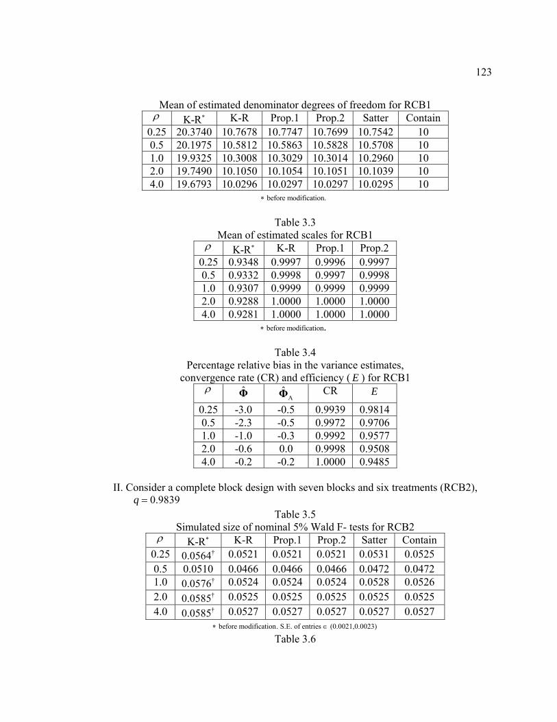
123

Mean of estimated denominator degrees of freedom for RCB1 ρ K-R∗ K-R Prop.1 Prop.2 Satter Contain

0.25 20.3740 10.7678 10.7747 10.7699 10.7542 10 0.5 20.1975 10.5812 10.5863 10.5828 10.5708 10 1.0 19.9325 10.3008 10.3029 10.3014 10.2960 10 2.0 19.7490 10.1050 10.1054 10.1051 10.1039 10 4.0 19.6793 10.0296 10.0297 10.0297 10.0295 10


Table 3.3 Mean of estimated scales for RCB1

ρ K-R∗ K-R Prop.1 Prop.2 0.25 0.9348 0.9997 0.9996 0.9997 0.5 0.9332 0.9998 0.9997 0.9998 1.0 0.9307 0.9999 0.9999 0.9999 2.0 0.9288 1.0000 1.0000 1.0000 4.0 0.9281 1.0000 1.0000 1.0000



convergence rate (CR) and efficiency ( E ) for RCB1 ρ Φ AΦ CR E

0.25 -3.0 -0.5 0.9939 0.9814 0.5 -2.3 -0.5 0.9972 0.9706 1.0 -1.0 -0.3 0.9992 0.9577 2.0 -0.6 0.0 0.9998 0.9508 4.0 -0.2 -0.2 1.0000 0.9485

II. Consider a complete block design with seven blocks and six treatments (RCB2),

0.9839q =Table 3.5

Simulated size of nominal 5% Wald F- tests for RCB2 ρ K-R∗ K-R Prop.1 Prop.2 Satter Contain

0.25 †0.0564 0.0521 0.0521 0.0521 0.0531 0.0525 0.5 0.0510 0.0466 0.0466 0.0466 0.0472 0.0472 1.0 †0.0576 0.0524 0.0524 0.0524 0.0528 0.0526 2.0 †0.0585 0.0525 0.0525 0.0525 0.0525 0.0525 4.0 †0.0585 0.0527 0.0527 0.0527 0.0527 0.0527

before modification. S.E. of entries (0.0021,0.0023)∗ ∈ Table 3.6

124

Mean of estimated denominator degrees of freedom for RCB2 ρ K-R∗ K-R Prop.1 Prop.2 Satter Contain

0.25 37.3202 28.5050 28.5173 28.5076 28.4925 28 0.5 37.1337 28.3205 28.3266 28.3218 28.3143 28 1.0 36.9442 28.1321 28.1335 28.1324 28.1307 28 2.0 36.8508 28.0386 28.0387 28.0386 28.0384 28 4.0 36.8226 28.0102 28.0102 28.0102 28.0102 28


Table 3.7 Mean of estimated scales for RCB2

ρ K-R∗ K-R Prop.1 Prop.2 0.25 0.9873 1.0000 0.9999 1.0000 0.5 0.9872 1.0000 1.0000 1.0000 1.0 0.9871 1.0000 1.0000 1.0000 2.0 0.9870 1.0000 1.0000 1.0000 4.0 0.9870 1.0000 1.0000 1.0000



convergence rate (CR) and efficiency ( E ) for RCB2 ρ Φ AΦ CR E

0.25 -0.4 0.0 0.9995 0.9922 0.5 -0.5 -0.3 0.9998 0.9887 1.0 -1.6 -1.6 1.0000 0.9857 2.0 0.9 0.9 1.0000 0.9844 4.0 0.7 0.7 1.0000 0.9840

8.3 Comments and Conclusion

The bias of the conventional estimator of the variance-covariance matrix of the

fixed effects estimator is large and negative in most cases as expected especially with

small values of ρ (e.g., table 2.5 and table 2.10). The bias was found to be effected by

three factors: , , and .q nρ When , , and/or .q nρ get larger, the bias decreases. This bias

is reduced to an acceptable level by using the adjusted estimator. As expected, when the

between-block variance increased, the estimate of the denominator degrees of freedom

125

decreased (e.g., tables 1.3, 2.2, and 3.1). This is because that the contribution of the

information from between blocks to estimate the fixed effects and their covariance matrix

gets smaller. Notice that for all approaches, the denominator degrees of freedom

estimates approach the Containment method’s estimate as ρ increases. In other words,

as ρ increases, the optimal approximate test approaches the Intra-block exact F-test where

the between-block information is not utilized.

In general, the K-R before modification does not perform as well as K-R after

modification. Before modification, the K-R method tends to be more liberal than K-R

after modification (e.g., table 3.1 and 3.5). Even though the K-R approach using the

conventional estimator of the variance-covariance matrix of the fixed effects estimator

give reasonable true levels (table 1.2), the approach is not appropriate since the

denominator degrees of freedom and the scale estimates were found to be negative for

some data sets. For PBIB1 design, and when ρ =0.25, a data set has -120.8 as an estimate

of the denominator degrees of freedom.

The K-R and the proposed methods perform well and similarly and the similarity

gets stronger when ρ gets larger (for BIB designs, the K-R and proposed methods are

identical). Their true levels tend to be more conservative with designs where the

efficiency factor is higher, and this is related to the small remaining bias in the adjusted

estimator of variance-covariance matrix of the fixed effects estimator in most cases. This

bias is not eliminated in the BIB designs where the efficiency factor is small and this

makes the K-R and the proposed methods’ true levels more liberal (e.g., tables 2.5, 2.10

and 2.15). Indeed, they perform better than other approaches in most cases except a few

cases that will be mentioned below.

The Satterthwaite approach was found to perform poorly for designs with small

values of , and q nρ where the true level tends to be too liberal (e.g., table 2.2). This

unwanted liberality of the true level is related to the negative large percentage relative

bias in the conventional estimator of the variance-covariance matrix of the fixed effects

estimator for the cases where we have small values of , and q nρ (e.g., table 2.5).

When , and/or q nρ get larger, the Satterthwaite method tends to be more conservative.

126

This is due to the relatively small values of the bias in the conventional estimate of the

estimator of the variance-covariance matrix of the fixed effects estimator (e.g., table 2.9).

Indeed, when and q ρ get larger, the Satterthwaite method tends to perform as well as

the K-R and the proposed methods regardless of the sample size (e.g., table 2.12).

For the cases where the Satterthwaite method performs poorly, the Containment

method was found to perform better than the Satterthwaite method generally (e.g., tables

1.2 and 2.2). Moreover, for the cases where the efficiency factors are large, and

and/or nρ get larger, the performance of the Containment method improves in the way

that it becomes as good as the K-R and the proposed methods (e.g., tables 2.12 and 2.22).

For the cases where the efficiency factor is relatively small, we found the Containment

method’s performance tends to be better than all other approaches including the K-R and

the proposed methods when ρ is relatively small (e.g., table 2.2).

127

9. CONCLUSION

9.1 Summary

The strength of Kenward and Roger’s approach comes from combining three

components where no other approach does: First, instead of approximating the Wald-type

statistic itself by an F distribution as in the Satterthwaite approximation, Kenward and

Roger considered a scaled form of the statistic that makes the approximation more

flexible since they approximate the denominator degrees of freedom and the scale as

well. Second, Kenward and Roger modified the procedure in such a way that they get the

right values for both the denominator degrees of freedom and the scale for the two special

cases considered in chapter 3. Third, the adjusted estimator of the variance-covariance

matrix of the fixed effects estimator, which is less biased than the conventional estimator,

as we saw in chapter 2, is used in constructing the Wald-type statistic.

F

F

In this thesis, by modifying certain steps in Kenward and Roger’s derivation, we

obtain two alternative methods which are similar to the K-R method but simpler in

derivation and application. Whenever the ratio of the two quantities derived in

chapter 3 is the same as for the two special cases, the K-R and the proposed methods are

identical. We also showed that the K-R and the proposed methods produce the right

values for the denominator degrees of freedom and the scale factor, not only in the

special cases, but also in three general models where we have exact F tests for fixed

effects.

1 and A 2A

A Wald-type statistic was constructed using the conventional, rather than the

adjusted, estimator of the variance-covariance matrix of the fixed effects estimator, and

then modified to attain the right values in the two special cases. Because was found to

be null in all cases with exact F tests considered in this thesis, the modification step was

problematic and this is consistent with the remark made by Kenward and Roger (1997).

3A

Another approach to obtain approximate F tests for fixed effects is the

Satterthwaite method. When a one-dimensional hypothesis is of interest, then the K-R,

the Satterthwaite, and the proposed methods produce the same estimate of the

128

denominator degrees of freedom, and the scale estimate is one. Even though the estimates

are the same, the Satterthaite and the K-R tests are not necessarily identical, and this is

true because in the K-R statistic, we use the adjusted estimator of the variance-covariance

matrix of the fixed effects estimator, whereas the conventional estimator is used in the

Satterthwaite test. However, in some cases like balanced mixed classification models

where the adjustment in the estimator of the variance-covariance matrix of the fixed

effects estimator is null, the Satterthwaite approach is identical to the K-R and the

proposed methods when testing a one-dimensional hypothesis. When we make inference

about a multidimensional hypothesis, we still have some cases where the K-R and the

Satterthwaite approaches produce the same estimate of the denominator degrees of

freedom, or are even identical approaches as in lemma 7.2.7.

In chapter 8, we conducted a simulation study for three kinds of block designs;

partially balanced block designs, balanced incomplete block designs, and complete block

designs with missing data. The K-R, the proposed, the Satterthwaite, and the

Containment methods were compared in the study. Three factors were considered in the

study: the variance components ratio, the efficiency factor, and the sample size. In most

cases, we found the K-R and the proposed methods performed as well as or better than

the other methods. For designs with small values for all the three factors, the

Satterthwaite method performed poorly. The true level was found to be quite liberal due

to the large bias in the conventional estimator of the variance-covariance matrix of the

fixed effects estimator. In some designs where the efficiency factor and the ratio of the

variance components are both relatively small, the K-R and the proposed methods were

found to be liberal. For those cases, the Containment method was found to work as well

as or better than all other approaches.

9.2 Future Research

In this thesis, some questions about the K-R and other methods used to make

inference about fixed effects in mixed linear models were answered. However, many

issues still need to be investigated. In chapter 3, we derived approximate expressions for

129

the expectation and variance of the Wald-type statistic using the conventional

estimator of the variance-covariance of the fixed effects estimator. However, as we saw

in section 4.4, it was problematic to use the special cases to modify the approach since

was null. As a matter of fact, it is also null in all three general models considered in

chapter 6. A possible direction for further research is to investigate if there is any case

where we have an exact F test and is not null, so that a better modification can be

accomplished. Two different ratios

F

3A

3A

1 2A A were found in the two special cases and in the

three general models considered in chapter 6. It is suggested to search if there is any case

where we have an exact F test and the ratio 1 2A A is different than the two ratios we had.

In case another ratio is found, it is suggested to use it in the modifying stage for the K-R

and the proposed methods.

In balanced mixed classification models, and in the general models considered in

sections 6.2 and 6.3, we noticed that the adjustment of the estimator of the variance-

covariance matrix of the fixed effects estimator is null. It would be interesting to

generalize these results.

When we make an inference about a multidimensional hypothesis of the fixed

effects, lemma 7.2.7 provide conditions where the K-R and the Satterthwaite approaches

produce the same estimate of the denominator degrees of freedom. It would be interesting

to investigate the possibility of other conditions that lead to the same result.

Finally, based on the theoretical derivation of the methods proposed in chapter 5,

and their simulation results for the block designs in chapter 8, these methods’

performances are expected to be comparable to the K-R method. A natural proposal is to

investigate the performance of these proposed methods in other different models.

130

BIBLIOGRAPHY

Anderson, T. (2003). An Introduction to Multivariate Statistical Analysis. New York: John Wiley & Sons.

Bellavance, F., Tardif, S. and Stephens, M. (1996). Tests for the Analysis of Variance of Crossover Designs with Correlated Errors. Biometrics 52, 607-612.

Birkes, D. (2004). Linear Model Theory Class Notes, Unpublished. Oregon State University.

Birkes, D. and Lee, Y. (2003). Adjusted Orthogonal Block Structure in Mixed Linear Models. Unpublished.

Birkes, D. (2006). Class Notes. Unpublished. Oregon State University.

Chen, X. and Wei, L. (2003). A Comparison of Recent Methods for the Analysis of Small-Sample Cross-Over Studies. Statistics in Medicine 22, 2821-2833.

Cochran, W. and Cox, G. (1975). Experimental Designs. New York: John Wiley & Sons.

Fai, C and Cornelius, P. (1996). Approximate F Tests of Multiple Degree of Freedom Hypotheses in Generalized Least Squares Analysis of Unbalanced Split-Plot Experiments. Journal of Statistical Computation and Simulation 54, 363-378.

Giesbrecht, F. and Burns, J. (1985). Two-Stage Anaysis Based on a Mixed Model: Large- Sample Asymptotic Theory and Small-Sample Simulation Results. Biometrics 41, 477-486

Gomes, E., Schaalje, G. and Fellingham, G. (2005). Performance of the Kenward-Roger Method when the Covariance Structure is Selected Using AIC and BIC. Communications in Statistics-Simulation and Computation 34, 377-392.

Graybill, F. and Wang, C. (1980). Confidence Intervals on Nonnegative Linear Cominations of Variances. Journal of the American Statistical Association 75, 869-873.

Green, P. (2001). On the Design of Choice Experiments Involving Multifactor Alternatives. Journal of Consumer Research 1, 61-68.

Harville, D. (1997). Matrix Algebra from a Statistician’s Prospective. New York: Springer.

Harville, D. and Jeske, D. (1992). Mean Squared Error of Estimation or Prediction Under a General Linear Model. Journal of the American Sataistical Association 87, 724- 731.

Huynh, H. and Feldt, L. (1970). Conditions Under Which Mean Square Ratios in Repeated Measurements Designs Have Exact F-Distributions. Journal of the American Statistical Association 65, 1582-1589.

131

Kackar, R. and Harville, D. (1984). Approximations for Standard Errors of Estimators of Fixed and Random Effect in Mixed Linear Models. Journal of the American Staistical Association 79, 853-862.

Kenward, M. and Roger, J. (1997). Small Sample Inference for Fixed Effects from Restricted Maximum Likelihood. Biometrics 53, 983-997.

Krzanowski, W. (2000). Principles of Multivariate Analysis. Oxford, U.K.: Oxford University Press.

Kuehl, R. (2000). Design of Experiments: Statistical Principles of Research Design and Analysis. Pacific Grove: Duxbury Press.

Mardia, K., Kent, J. and Bibby, J. (1992). Multivariate Analysis. New York: Academic Press.

Pase, L. and Salvan, A. (1997). Principles of Statistical Inference. New Jersey: World Scientific.

Prasad, N. and Rao, J. (1990). The Estimation of the Mean Squared Error of Small-Area Estimators. Journal of the American Statistical Association 85, 163-171.

Pukelsheim, F. (1993). Optimal Design of Experiments. New York: John Wiley & Sons.

Rady, E. (1986). Testing Fixed Effects in Mixed Linear Models. Ph.D. thesis, Unpublished. Oregon State University.

Rao, C. (2002). Linear Statistical Inference and its Applications. New York: John Wiley & Sons.

SAS Institute, Inc. (2002-2006), SAS version 9.1.3, Online Help, Cary, NC: SAS Institute.

Satterthwaite, F. (1941). Synthesis of Variance. Psychometrika 6, 309-316.

Satterthwaite, F. (1946). Approximate Distribution of Estimates of Variance Components. Biometrics 2, 110-114.

Savin, A., Wimmer, G. and Witkovsky, V. (2003). Measurement Science Review 3, 53- 56.

Schaalje, G., McBride, J. and Fellingham, G. (2002). Journal of Agricultural, Biological, and Enviromental Statistics 7, 512-524.

Schott, J. (2005). Matrix Analysis for Statistics. New York: John Wiley & Sons.

Searle, S., Casella, G. and McCullouch, C. (1992). Variance Components. New York: John Wiley & Sons.

Seely, J. (2002). Linear Model Theory Class Notes, Unpublished. Oregon State University.

132

Seely, J. and Rady, E. (1988). When Can Random Effects Be Treated As Fixed Effects For Computing A Test Statistic For A Linear Hypothesis? Communications in Statistics- Theory and Methods 17, 1089-1109.

Siefert, B. (1979). Optimal Testing for Fixed Effects in General Balanced Mixed Classification Models. Math. Operationsforsh. Statist. Ser. Statistics 10, 237-256.

Spike, J., Piepho, H. and Meyer, U. (2004). Approximating the Degrees of Freedom for Contrasts of Genotypes Laid Out as Subplots in an Alpha-Design in a Split-Plot Experiment. Plan Breeding 123, 193-197.

Utlaut, T., Birkes, D. and VanLeeuwen, D. (2001). Optimal Exact F Tests and Error- Orthogonal Designs. Conference Proceeding of the 53rd ISI Session, Seoul 2001.

VanLeeuwen, D., Seely, J. and Birkes, D. (1998). Sufficient Conditions for Orthogonal Designs in Mixed Linear Models. Journal of Statistical Planning and Inference 73, 373-389. VanLeeuwen, D., Birkes, D. and Seely, J. (1999). Balance and Orthogonality in Designs for Mixed Classification Models. The Annals of Statistics 27, 1927-1947.

kenward â€“ roger's approach - oregon state university

Documents