CHALLENGES IN POLYMERIZATION REACTOR MODELING AND OPTIMIZATION: A POPULATION BALANCE PERSPECTIVE

Costas Kiparissides

Department of Chemical Engineering, Aristotle University of Thessaloniki & Chemical Process Engineering Research Institute, P.O. Box 472, 54006, Thessaloniki, Greece

Abstract: In the present article, recent developments on modeling, monitoring, optimization and control of particulate polymerization processes are reviewed. A unified population balance approach is described to follow the time evolution of molecular and morphological polymer properties in batch and continuous polymerization reactors. Recent advances on the online monitoring of “polymer quality” are discussed in the context of available hardware and software sensors. The problem of real-time optimization of polymerization processes under parametric uncertainty is also examined along with its online implementation. Finally, new issues related with the modeling, numerical solution and control of multidimensional PBEs are conferred. Copyright © 2004 IFAC Keywords: Polymerization, Particulate processing, Product quality, Distributions, Computational methods, Estimators, Optimization, Control

1. INTRODUCTION Process modeling, optimization and control can have a significant impact on polymer plant operability and economics. Polymer manufacturers face increasing pressures for production cost reductions and more stringent quality requirements. However, product quality in polymer manufacturing is a much more complex issue than in more conventional simple chemical systems. Thus, a major objective of polymerization reactor modeling is to understand how the reaction mechanism, the physical transport phenomena (e.g., mass and heat transfer), mixing, reactor type and operating conditions affect the “polymer quality”. The last term includes all the polymer molecular properties (e.g., molecular weight distribution (MWD), copolymer composition distribution (CCD), sequence length distribution (SLD), long and short chain branching distributions (SCB, LCB), stereoregularity, etc.) as well as the morphological properties of the product (e.g., particle size distribution, (PSD), pore size distribution, bulk density, etc.). One of the most difficult issues in polymer reactor optimization and control is to determine the quantitative relationships between the product physical, thermal, mechanical,

rheological, chemical properties and the molecular/morphological polymer properties. Table 1 summarizes both types of quality control measures. Since the end-use properties of the produced polymers are directly linked with the molecular characteristics of the polymer chains, control of the polymer chain microstructure is of profound interest to the polymer manufacturing industry. This presupposes a thorough knowledge of the polymerization kinetics and the availability of advanced mathematical models to quantify the effects of process operating conditions on the molecular and morphological polymer properties. A great number of modeling studies on the prediction of MWD, CCD, PSD, etc. for linear and branched polymers have been published. Most of the models follow the general framework of population balances but having as internal coordinates the chain length, the chain composition, etc. of the polymer molecules or the particle volume. Synthetic polymers are produced via a multitude of reaction mechanisms (e.g., free-radical, catalytic, ionic, etc.) and processes (e.g., bulk, solution, suspension, etc.). In general, polymerization

Table 1. Some Measures of Polymer Product Quality

MOLECULAR AND MORPHOLOGICAL PROPERTIES END-USE PROPERTIES

••

•• •• •• •• •• ••

••

•• ••

••

Average Molecular Weights and Molecular Weight Distribution (MWD) Copolymer Composition Distribution (CCD) Sequence Length Distribution (SLD) Long-Chain Branching Distribution (LCBD) Stereoregularity (Tacticity) Particle Size Distribution (PSD) Particle Porosity and Surface Area, etc.

Physical and thermal properties (e.g., density, clarity, melting point, temperature stability, swellability, plasticizer uptake, etc.) Chemical (e.g., corrosion resistance, etc.) Mechanical properties (e.g., strength, toughness, stress crack resistance, abrasion resistance, impact resistance, etc.) Rheological properties (e.g., flow properties, shear viscosity and elasticity, melt index, extensional viscosity, extrudate swell, etc.)

processes can be broadly classified into homogeneous and heterogeneous ones. The first class comprises polymerizations which are carried our in a single phase. The latter involves the presence of several phases (i.e., solid, liquid and gas). In heterogeneous polymerization, the final product is obtained in the form of a distribution of polymer particles in the sub-micron or micron size range. Table 2 presents the main characteristics of typical particulate polymerization processes employed for the production of some well-known commodity polymers (Kiparissides, 1996). The analysis of particulate polymerization processes is a rather complex problem due to the highly coupled kinetics, thermodynamics, heat and mass transfer phenomena, taking place in a heterogeneous process. Furthermore, the physical properties (e.g., viscosity, density, transport coefficients, interfacial tension, etc.) of the various phases typically vary by several orders of magnitude in the course of polymerization. Thus, the framework of population balances is ideally suited to the description of the complex dynamics of a wide range of particulate polymerization processes. Efficient polymer reactor process control requires correct information on the state of the polymerization process. Therefore, the availability of on-line measurements is an essential requirement for the implementation of high-level process and polymer quality optimization schemes. On-line monitoring devices have to be able to measure continuously (or at least semi-continuously) and often condition the

sampled material (and sometimes even chemically process it); they must have a satisfactory analysis and response time behaviour; and, finally, they have to supply correct results over long periods of time in environments that are often physically and chemically aggressive. In a review article (Kammona, et al., 1999), a comprehensive survey on recent advances on hardware and software sensors for on-line monitoring of polymer quality was presented. The operating objectives in batch and continuous polymerization processes must satisfy complex molecular and morphological property requirements for the final product and simultaneously achieve the greatest economic potential for the plant. Basically, two types of optimization problems are encountered in polymerization processes. The first deals with the selection of the best (optimal) time invariant controls so that, in the absence of process disturbances, the final product attains some desired molecular and morphological properties. The second, the time optimal control problem, deals with the calculation of the time-optimal control trajectories to ensure the satisfaction of the “polymer quality” requirements and the operational process constraints. These optimal control policies can be calculated offline and implemented as set-point changes of the regulatory process controllers. However, the operation of a polymerization process is heavily affected by disturbances (e.g., process-related sources or inherent model parameter uncertainties) that cause the process to drift away from the offline

Table 2. Typical Particulate Polymerization Processes

Kinetic Mechanisms: FR – Free Radical, I- Ionic, ZN- Ziegler-Natta Polymers: PS – Polystyrene, PMMA – Poly(methyl methacrylate), PVA – Poly(vinyl acetate), PVC – Poly(vinyl cloride), HDPE – High density polyethylene, LLDPE – Linear low density polyethylene, PTFE – Poly(tetrafluorethylene), PP – Polypropylene, EP – Ethylene- Propylene copolymers

Process: Suspension Emulsion Precipitation Liquid Slurry

Gas-Solid Polymerization

Particle Size (µm) 50-500 0.1-1.0 100-104 10-104 10-104 Reactor Type Batch Batch,

CSTR Batch, CSTR

Batch, Loop

Fluid Bed, Stirred Bed

Kinetic Mechanism FR, I FR, I All ZN ZN Polymers PMMA

PS, PVC PS, PMMA, PVA, PTFE

PVC, PTFE

HDPE, PP, EP

HDPE, PP, LLDPE, EP

calculated optimal trajectories. To alleviate the above problems, an online estimation-optimization approach needs to be implemented (Kiparissides, et al., 2002, Chatzidoukas, et al., 2003). The updating of the time optimal control policies is carried out in two steps: in the first step, a state/parameter estimator utilizes the available process measurements to obtain reliable estimates of the state variables and the time-varying model parameters. In the optimization step, the time optimal trajectories are periodically reevaluated based on the most recent information about the process. The calculation of the time optimal control policy is obtained via dynamic programming techniques (including sequential and simultaneous discretization methods). The present paper deals with the modeling and optimization of particulate polymerization processes using a population balance approach. In particular, the paper addresses the following topics. In section two, a unified population balance approach is presented to follow the molecular weight (e.g., MWD, LCB, etc.) and morphological (e.g., PSD) changes in a particulate polymerization process. The solution of the general PBE is reviewed in relation to available numerical methods (e.g., M-I and M-II approaches, finite differences, collocation, finite elements, wavelets, etc.). Subsequently, the general population balance approach is applied to typical polymerization processes to predict the dynamic evolution of MWD, PSD, etc. in batch and continuous systems. In section three, the calculation of the time optimal control policies under structural and parametric uncertainty is reviewed along with their on-line implementation to polymerization processes. Finally, in section four, future directions related to the modeling, monitoring, optimization and control of particulate polymerization reactors are conferred.

2. THE POPULATION BALANCE EQUATION The development of the general population balance equation (PBE) follows the works of Hulburt and Katz (1964) and Ramkrishna (1985). Let us consider a distribution of countable entities (e.g., polymer chains, monomer droplets, polymer particles, etc.)

where and represent ordinary spatial coordinates, is the time, and represents the ith property of the entity. For example,

could denote the degree of polymerization, or the comonomer composition or the volume of a polymer particle. Actually, the term represents the fraction of entities in the geometric volume element

( )t,p,...p,p,z,y,xn k21

ip

V

y,x

n

z

dxdydzdp

t ip

kdp1...

zyx δδδ

2 ... ,pn

=δ

1 ,p δδ, with property values

in the range . Note that the distribution function will satisfy the following condition:

kpδ

(1) ( ) 1dp ... dpdp dxdydzp,...p,p,z,y,xn k21k21 =∫In the above formulation, there are (3 + k) independent variables plus time involved that can be viewed as a (3 + k) dimensional space. Thus, for an

ordinary small volume element in this space, Ω , the general population balance becomes (Himmelblau and Bischoff, 1968):

( )∫∫ΩΩ

Ω−=Ω dDBnddtd (2)

where

(3) ∫ ∫ ∫∫ ∫ ∫Ω

==Ωx py z p

k21k1

... ; dp ... dpdxdydzdpd

B and represent the corresponding rate of “birth” and “death” of entities per unit time, unit geometric volume and unit property change. The left-hand side of eq (2) can be modified by using the general form of Leibnitz’s rule for differentiating definite integrals. Thus, following the general developments of Himmelblau and Bischoff, the differential form of eq (2) can be obtained:

D

( ) ( ) ( )

( ) 0BDnup

nuz

nuy

nuxt

n

i

k

1i i

zyx

=−+∂∂

+

+∂∂

+∂∂

+∂∂

+∂∂

∑=

(4)

where ux = dx/dt, uy = dy/dt and uz = dz/dt denote the usual geometric velocities in the spatial coordinates, respectively.

z and y ,xdtidpu i =

i

is the rate of change of the property p . Very often, the average values of the properties in the entire reactor volume,

, are only required. Accordingly, one can define the following geometrically averaged distribution function,

V

n .

∫=V

ndVV1n (5)

By integrating eq (4) over the geometric volume, V , and using the Gauss’ divergence theorem, the following macroscopic population balance equation is obtained:

( ) ( )

( )outoutinin

i

k

1i i

nqnqV1

BDnup

nVtV

1

−=

=−+∂∂

+∂∂ ∑

= (6)

where and q are the inlet and outlet volumetric flow rates, respectively.

inq out

2.1 Calculation of Molecular Weight Distribution Let us assume that the kinetic mechanism of the chemically initiated free-radical polymerization of a vinyl monomer comprises the following elementary reactions: Initiator decomposition:

•→ R2I dk Chain initiation:

1k RMR I→+•

Propagation:

1xk

x RMR p+→+

Chain transfer to monomer:

1xk

x RPMR fm + →+

Chain transfer to solvent (CTA):

1xk

x RPSR fs +→+

Termination by disproportionation:

yxk

yx PPRR td +→+

Termination by combination:

yxk

yx PRR tc+→+

Chain transfer to polymer:

xyk

yx PRPR fp +→+

Reaction with terminal double bond:

yxk

yx RPR db+

= →+ The subscripts x and y denote the number of monomer units in a polymer chain. The above kinetic mechanism includes propagation and termination reactions by both disproportionation and combination, molecular weight control reactions via transfer to monomer and to chain transfer agent, long-chain branching formation by transfer to polymer and reaction with terminal double bonds. Based on the above kinetic mechanism, we can derive the following population balance equations for the “live”, R , and “dead”, , polymer chains of length . Assuming that the degree of polymerization, , can only take discrete values

, the inlet and outlet terms in eq (6) are equal to zero (i.e., batch reactor) and the rate of change of property is equal to zero, one can easily derive the following macroscopic population balances for the entities

( t,xx

x)

x

) )( t,xP

( fN ... ,2,1:x

( )t,xR and P . ( )t,x

( ) [ ][ ] [ ] [ ]( ) ( )

( ) ( ) [ ] [ ] [ ] (

( ) ( ) ( ) ( )

( ) ( ) ( ) ( )

( ) ( ) ( ) ( )∑∑

∑∑

∑∑

∑

−

=

∞

=

∞

=

∞

=

∞

=

∞

=

∞

=

•

−−+−−

−−−

−−−+

++−−−+

+δ

++=

1x

1ydb

2ydb

1ytc

1ytd

2yfp

1yfp

fsfmp

1,x1y

fsfmI

t,yxDt,yxRk t,yxDt,xRk

)7(t,yRt,xRkt,yRt,xRk

t,yxyDt,xRkt,yRt,xDxk

t,xRSkMk Mt,xRt,1xRk

t,xRSkMkMRkVRdtd

V1

)

( ) [ ] [ ] ( )

( ) ( ) ( ) ( )

( ) ( ) ( ) ( )

( ) ( ) )8(t,yRt,xDk

t,yxRt,yRk21t,yRt,xRk

t,yxDyt,xRkt,yRt,xDxk

t,xRSkMkVPdtd

V1

1ydb

1x

1ytc

1ytd

2yfp

1yfp

fsfm

∑

∑∑

∑∑

∞

=

−

=

∞

=

∞

=

∞

=

−

−−++

+−+−

−+=

where is the Kronecker’s delta function (i.e.,

if and 1,xδ

1 x1,x =δ 1= 01,x =δ if ). 1x ≠Note that the right-hand side terms in eqs (7-8) represent the net production rates of “live” and

“dead” polymer chains. The actual number of rate equations for the “live” and “dead” polymer chains will depend on the total degree of polymerization, Nf, that may be of the order of hundreds or/and thousands monomer units. Consequently, the computational effort associated with the solution of the complete set of differential equations becomes prohibitively high for most cases of interest and makes the on-line application of such a model unrealistic. To deal with the above high-dimensionality problem, several methods have been proposed to reduce the infinite system of differential equations into a low-order system of DAEs. These can be broadly classified into kinetic lumping methods, continuous variable approximations, z-transforms, method of moments, discrete weighted Galerking, orthogonal collocation on finite elements and so forth. In the kinetic lumping methods (Crowley and Choi, 1997a,b, 1998), the polymer chains population is divided into a specified number of “chain lump” domains and the resulting population balance equations are solved numerically. A uniform concentration is assumed for all polymer chains that are members of a “chain lump” domain. However, the calculation of MWD for branched polymers (e.g., systems involving transfer to polymer and terminal double bond reactors) suffers from significant inaccuracies. Continuous variable approximation and z-transform methods, besides their elegant mathematical formulation, lack the ability to handle complex polymerization systems efficiently. Polynomial expansion methods of the MWD require the calculation of high-order moments and may lead to slow convergence (Tobita and Ito, 1993). Pladis and Kiparissides (1998) proposed a polymer chain fractionation approach and used the method of moments to reconstruct the joint molecular weight – long-chain branching distribution for branched polymers. The total population of the polymer chains was divided into a number of classes with respect to the number of long-chain branches. However, in addition to the well-known problem of closure of the “higher-order” moments, the reconstruction of the overall MWD at high monomer conversions and high LCB content requires a very large number of classes to reduce the approximation errors for high molecular weight fractions. Monte-Carlo simulations (Tobita, 1993, 1995) are straightforward techniques that can generally handle complex kinetic mechanisms but usually require significant computational effort for the determination of the MWD. Discrete weighted Galerkin formulation (Deuflhard and Wulkow, 1989, Wulkow, 1992), even though are computationally demanding, provide a powerful tool for the prediction of the MWD in complex polymerization systems (Iedema et al., 2000). However, the approximation of the infinite summation terms (e.g., resulting from termination by combination reactions) requires special treatment. Method of Moments. The method of moments is based on the statistical representation of the average molecular properties of the polymer (e.g., number average, Mn, and weight average, Mw, molecular weights) in terms of the leading moments of the

number chain length distributions (NCLDs) of “live” and “dead” polymer chains, defined by the following equations:

(9) 2,1,0k,Px,Rx1x

xk

k1x

xk

k ==µ=λ ∑∑∞

=

∞

=

The relevant rate functions for the moments of the NCLDs of the “live” and “dead” polymer chains can be obtained by multiplying each term of eqs (7-8) by xk and summing the resulting expressions over the total degree of polymerization, N∝. The resulting rate equations for the leading moments are (Pladis and Kiparissides, 1998):

[ ][ ] [ ] [ ]

[ ] [ ] [ ]

[ ]

)10(kk

kkkSk

MkMkik

Mk

SkMkMRkdt

d

k0t

k

0iikidb

0kdb1k0fp1kfpkfs

kfmkp

k

0iip

0fs0fmIk

λλ−µλ+

+µλ−µλ+µλ−λ−

−λ−λ−λ

+

+λ+λ+=λ

∑

∑

=−

+

=

•

[ ] [ ]

k0td

k

0iikitck0db1k0fp

1kfpkfskfmk

kik

k21kk

)11(kSkMkdt

d

λλ+λλ

+µλ−µλ−

−µλ+λ+λ=µ

∑=

−+

A set of residual equations are then derived by substituting eqs (12-13) into eqs (7-8). The main requirement of the OCFE formulation forces the residual balances to vanish at the selected collocation points, si,j. The number of the finite element controls the density of the collocation points in the overall chain length domain. In general, a high density of collocation points is required in chain length regions where steep changes in the concentrations of “live” and “dead” polymer chains are foreseen. Extensive simulations showed that low-order interpolation polynomials predict the overall MWD more accurately, compared to high-order polynomials for the same total number of collocation points. This was attributed to the oscillatory behavior of the high-order Langrange polynomials.

where [ ]•R , and denote the concentrations of “live” radicals, monomer and chain transfer agent, respectively. Usually, one needs to know the leading moments (i.e., λ

[ ]M [ ]S

0, λ1, λ2 and µ0, µ1, µ2 of the “live” and “dead” polymer distributions) to calculate the values of the number-average, Mn, and weight-average, Mw, molecular weights. Orthogonal Collocation on Finite Elements. A key characteristic of the OCFE method is the treatment of the discrete polymer chain length domain as a continuous one. Hence, the concentrations of “live” and “dead” polymer chains are handled as continuous variables. Accordingly, the chain length domain is divided into a number of finite elements, NE, with element boundaries at the points: ζ0=1, ζ1, ζ2,…, ζNE-1, ζNE = Nf, where Nf is the final degree of polymerization. For each element, a number of n interior collocation points, [s1, s2,…, sn] are specified. The concentrations of the “live” and “dead” polymer chains are then approximated by continuous low-order polynomial functions within each finite element. In the present study, Lagrange interpolation polynomials were used to approximate the concentrations of the “live” and “dead” polymer chains:

(12) ( ) ( ) ( )∑=

− =ζ≤≤ζ=n

0ij1jj,i

Rj,i NE,,1jssR~sWsR~ …

(13) ( ) ( ) ( ) NE,,1jssP~sWsP~n

1ij1jj,i

Pj,i …=ζ≤≤ζ= ∑

=−

The tilde denotes approximation variables. The functions, and are Lagrange

interpolation polynomials of order n+1 and n, respectively, given by the expressions:

( )sW Rj,i ( )sW P

j,i

( )

NE,,1jn,,0i

sss

sssW j1j

n

0k j,kj,i

j,kRj,i

ik

…… ==

ζ≤≤ζ−

−= −

=∏

≠ (14)

( )

NE,,1jn,,1i

sss

sssW

n

1kj1j

j,kj,i

j,kPj,i

ik

…… ==

ζ≤≤ζ−

−=∏

≠=

− (15)

The Lagrange polynomials and ( )sW Rj,i ( )sW P

j,i are equal to zero at the collocation points si,j, for k≠i and equal to unity for k=i. To take into account the concentration of “live” polymer chains at chain length x=1, the left boundary point of the first element was included as an interpolation point.

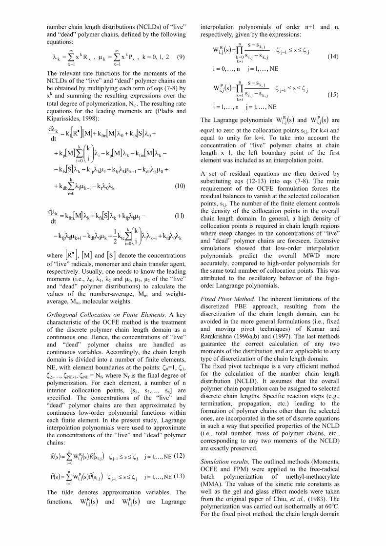
Fixed Pivot Method. The inherent limitations of the discretized PBE approach, resulting from the discretization of the chain length domain, can be avoided in the more general formulations (i.e., fixed and moving pivot techniques) of Kumar and Ramkrishna (1996a,b) and (1997). The last methods guarantee the correct calculation of any two moments of the distribution and are applicable to any type of discretization of the chain length domain. The fixed pivot technique is a very efficient method for the calculation of the number chain length distribution (NCLD). It assumes that the overall polymer chain population can be assigned to selected discrete chain lengths. Specific reaction steps (e.g., termination, propagation, etc.) leading to the formation of polymer chains other than the selected ones, are incorporated in the set of discrete equations in such a way that specified properties of the NCLD (i.e., total number, mass of polymer chains, etc., corresponding to any two moments of the NCLD) are exactly preserved. Simulation results. The outlined methods (Moments, OCFE and FPM) were applied to the free-radical batch polymerization of methyl-methacrylate (MMA). The values of the kinetic rate constants as well as the gel and glass effect models were taken from the original paper of Chiu, et al., (1983). The polymerization was carried out isothermally at 60oC. For the fixed pivot method, the chain length domain

1 10 100 1000 10000 1000000,00

0,02

0,04

0,06

0,08

0,10

0,12

0,14

0,16

Conversion = 93 %

Conversion = 91 %

Conversion = 85 %

Conversion = 30 %

Wei

ght (

gr/lt

)

Chain Length

Fig. 1. Time evolution of the MWD calculated by the FP method.

1 10 100 1000 10000 100000

0,00

0,02

0,04

0,06

0,08

0,10

Wei

ght (

gr/lt

)

Chain Length

Fixed Pivot Predici

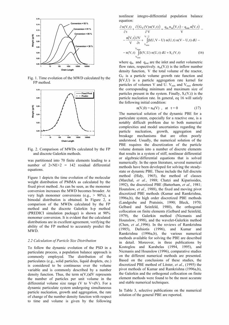
Fig. 2. Comparison of MWDs calculated by the FP and discrete Galerkin methods.

was partitioned into 70 finite elements leading to a number of 2×NE+2 = 142 residual differential equations. Figure 1 depicts the time evolution of the molecular weight distribution of PMMA as calculated by the fixed pivot method. As can be seen, as the monomer conversion increases the MWD becomes broader. At very high monomer conversions (e.g., > 90%), a bimodal distribution is obtained. In Figure 2, a comparison of the MWDs calculated by the FP method and the discrete Galerkin h-p method (PREDICI simulation package) is shown at 90% monomer conversion. It is evident that the calculated distributions are in excellent agreement, verifying the ability of the FP method to accurately predict the MWD.

2.2 Calculation of Particle Size Distribution

To follow the dynamic evolution of the PSD in a particulate process, a population balance approach is commonly employed. The distribution of the particulates (e.g., solid particles, liquid droplets, etc.) is considered to be continuous over the volume variable and is commonly described by a number density function. Thus, the term n(V,t)dV represents the number of particles per unit volume in the differential volume size range (V to V+dV). For a dynamic particulate system undergoing simultaneous particle nucleation, growth and aggregation, the rate of change of the number density function with respect to time and volume is given by the following

nonlinear integro-differential population balance equation:

( ) ( ) ( )

( )

)16()t,V(SdU)t,U(n)U,V()t,V(n

dU)t,UV(n)t,U(n)UV,U(tV

Vt,Vn

Vt,Vnqt,Vnq

V)t,V(n)V(G

t)t,V(n

v

V

V

2/V

V

outininV

max

min

min

+β−

−−−β+∂∂

−

−−

=∂

∂+

∂∂

∫

∫

where qin and qout are the inlet and outlet volumetric flow rates, respectively. nin(V,t) is the inflow number density function, the total volume of the reactor, G

VV is a particle volume growth rate function and

β(V,U) is a particle aggregation rate kernel for particles of volumes V and U. Vmin and Vmax denote the corresponding minimum and maximum size of particles present in the system. Finally, Sv(V,t) is the particle nucleation rate. In general, eq 16 will satisfy the following initial condition: n(V,0) = n0(V) , at t = 0 (17) The numerical solution of the dynamic PBE for a particulate system, especially for a reactive one, is a notably difficult problem due to both numerical complexities and model uncertainties regarding the particle nucleation, growth, aggregation and breakage mechanisms that are often poorly understood. Usually, the numerical solution of the PBE requires the discretization of the particle volume domain into a number of discrete elements that results in a system of stiff, nonlinear differential or algebraic/differential equations that is solved numerically. In the open literature, several numerical methods have been developed for solving the steady-state or dynamic PBE. These include the full discrete method (Hidy, 1965), the method of classes (Marchal, et al., 1988; Chatzi and Kiparissides, 1992), the discretized PBE (Batterham, et al., 1981; Hounslow, et al., 1988), the fixed and moving pivot discretized PBE methods (Kumar and Ramkrishna, 1996a,b), the high order discretized PBE methods (Landgrebe and Pratsinis, 1990; Bleck, 1970; Gelbard and Seinfeld, 1980), the orthogonal collocation on finite elements (Gelbard and Seinfeld, 1979), the Galerkin method (Nicmanis and Hounslow, 1998), and the wavelet-Galerkin method (Chen, et al.,1996). In the reviews of Ramkrishna (1985), Dafniotis (1996), and Kumar and Ramkrishna (1996a,b), the various numerical methods available for solving the PBE are described in detail. Moreover, in three publications by Kostoglou and Karabelas (1994, 1995), and Nicmanis and Hounslow (1996), comparative studies on the different numerical methods are presented. Based on the conclusions of these studies, the discretized PBE method of Litster, et al., (1995) the pivot methods of Kumar and Ramkrishna (1996a,b), the Galerkin and the orthogonal collocation on finite element methods were found to be the most accurate and stable numerical techniques. In Table 3, selective publications on the numerical solution of the general PBE are reported.

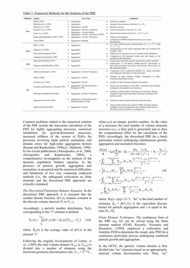
Table 3. Numerical Methods for the Solution of the PBE

Methods Author Test Cases Comments Hiddy (1965) Aggregation • Full discrete method. Batterham et al. (1981) Aggregation • Geometric discretization of the form Vi+1=2Vi. Marchal et al. (1988) Aggregation / Growth • Method of classes. Hounslow et al. (1988) Aggregation / Growth / Nucleation • Fixed discretization of the form Vi+1=2Vi.

≥

Common problems related to the numerical solution of the PBE include the inaccurate calculation of the PSD for highly aggregating processes, numerical instabilities for growth-dominated processes, increased stiffness of the system of DAEs for processes involving rapid particle nucleation, and domain errors for high-order aggregation kernels (Kumar and Ramkrishna, 1996a,b ; Dafniotis, 1996). In two recent publications (Alexopoulos, et al., 2004; Alexopoulos and Kiparissides, 2004), a comprehensive investigation on the solution of the dynamic population balance equation, in the presence of particle growth, aggregation and nucleation, is presented and the numerical difficulties and limitations of two very commonly employed methods (i.e., the orthogonal collocation on finite elements and the discretized PBE approach) are critically examined. The Discretized Population Balance Equation. In the discretized PBE approach, it is assumed that the number density function, n(V,t), remains constant in the discrete volume interval (Vi to Vi+1). Accordingly, a particle number distribution, Ni(t), corresponding to the “i” element is defined:

(∫+

−== +

1i

i

V

Vi1iii VV)t(ndV)t,V(n)t(N ) (18)

where in (t) is the average value of n(V,t) in the element “i”. Following the original developments of Litster, et al., (1995) the total volume domain (Vmin to Vmax) is divided into a number of elements using the fractional geometric discretization rule, Vi+1 = 21/q

Vi ,

where q is an integer, positive number. As the value of q increases the total number of volume elements increases (i.e., a finer grid is generated) and so does the computational effort for the calculation of the PSD. Accordingly, the discretized PBE for a batch particulate system undergoing simultaneous growth, aggregation and nucleation becomes:

∑∑

∑ ∑

∑

∑ ∑

∑

−−

=−−

+−∞

+−=

−−−

=

+−+−−

+−+−−=+−+−

−−

=−−−

−−+−

=

−+−−

+−+−−=−−

+−

=

β−

+β−

−−−−

β+

+−

β−β+

+−+−

β+

+

−−+

−++−δ=

1)q(Si

1jj1ij,1iq/1

q/)1ij(

1)q(Sijjij,i

q/1

q/)1k(q/)ij(q/1q

2k

1k)1kq(Si

2k)2kq(Sijj1kij,1ki

q/1

q/)ij()q(Si

1jjij,i

2qiqi,qi

q/1

q/)1k(q/)1ij(q

2k

k)1kq(Si

1k)2kq(Sijjkij,ki

21i

i21i

i

Vi

3

1j0

i

NN12

2 NN

12222NN

)19( 12

2NNN21

12212NN

rr

NN 1r

NrV)r1(3

G2 f)ji()t(S dt

)t(Nd

where S 2/)1q(q)q( += . “ne” is the total number of elements, βi,j = β(Vi,Vj) is the equivalent discrete kernel for particle aggregation and r is equal to the ratio Di+1/Di.

Finite Element Techniques. The continuous form of the PBE (eq 16) can be solved using the finite element method (FEM). Recently, Nicmanis and Hounslow, (1998), employed a collocation and Galerkin FEM to determine the steady state PSD for a continuous particulate process undergoing combined particle growth and aggregation. In the OCFE, the particle volume domain is first divided into “ne” elements based on an appropriately selected volume discretization rule. Then, “nc”

Litster et al. (1995) Aggregation / Growth (Batch) Aggregation / Growth / Nucleation (CSTR)

• Discretization based on the rule Vi+1=2Vi.1/q, q 2

Kumar and Ramkrishna (1996a,b; 1997) Aggregation / Growth / Nucleation • Arbitrary discretization.

M-I

Vanni (2000) Aggregation /Breakage • Comparison of DPBE methods based on a very coarse discretization

Bleck (1970) Aggregation • Use of two different types of discretization. (i.e . Vi+1=21/2 Vi and Vi+1=21/3 Vi).

Gelbard et al (1980) Aggregation • Generalization for the multi-component PBE case (Gelbard and Seinfeld, 1980).

Satry and Gaschignard (1981) Aggregation • Different set of equations for every moment of the distribution. M-II

Landgrebe and Pratsinis (1990) Aggregation • Comparison of the numerical results only with respect to the moments of the distribution.

Sigh and Ramkrishna (1975) Aggregation • Employment of problem-specific polynomials as basis functions.

WR Sampson and Ramkrishna (1985) Aggregation

• Employment of root-shifted problem-specific polynomials as basis functions.Improved accuracy based on the correct choice of the collocation points

Gelbard and Seinfeld (1978) Aggregation / Growth / Nucleation • Comparison of two collocation methods (i.e., spline collocation and orthogonal collocation on finite elements).

Pillinis (1990) Aggregation / Growth • Galerkin on finite elements method. Simulations of multi-component particulate systems.

Erasmus et al. (1994) Aggregation / Growth • Galerkin on finite elements method with b-splines.

Nicmanis and Hounslow (1996 and 1998) Aggregation / Growth /Nucleation / Breakage (CSTR)

• Steady state formulation of the PBE. Collocation and Galerkin techniques with quadratic basis functions.

Mahoney and Ramkrishna (2002) Aggregation / Growth / Nucleation • Galerkin on finite elements with linear basis functions. Special

treatment of moving discontinuities that arise in problems with particle growth.

Rigopoulos and Jones (2003) Aggregation / Growth /Nucleation / Breakage (Batch, CSTR) • Galerkin on finite elements with linear basis functions.

FE

Sandu and Borden (2003) Aggregation / Growth • General framework for the solution of PBE with finite element

techniques. Several formulations are considered with respect to the choice of basis functions, co-ordinates etc.

internal collocation points are specified within each element. Accordingly, the unknown number density function is approximated at the internal and boundary collocation points of each element, “e”, in terms of Lagrange basis functions, φj,:

(20) )V()t(n)t,V(n j

1nc

0j

ej ϕ= ∑

+

=

where denotes the value of n(V, t) at the “j” internal or boundary collocation point. The above approximation, results in a total number of (ne(nc+1)+1) unknown values of the number density function, .

ejn

nej

Following the general developments of Finlayson (1980), eq 16, for a batch process, can be recast into a system of (ne•nc) residual equations, corresponding to all the internal points of the “ne” volume elements.

( ) ( ) ( )

[

)21(dV)VV(n)V(n)V,VV(

)VV(nn)V,VV(Jw

tnV,VJwtn-

)t(ndV

dG )V(GJ)t(ndd

)t(n

ei

2/V

V

ei

1g

1f

nc

1j

fj

ei

ei

fj

fj

ei

fGj

ne

1f

fk

fk

ei

nc

1k

fGk

ei

ei

i

ViV

eej

i

1nc

0j

jei

ei

g1

−−β+

+−−β+

+β

−

−

ξ

ϕ−=

∫

∑∑

∑ ∑

∑

−

= =

= =

+

=

2/Vei

]

According to the standard finite element formulation, the global volume domain of each element “e” is linearly transformed into a local domain [-1,1]. The index “g” denotes the element containing the ( )

discrete point. fJ is the Jacobean of the volume transformation and wk

G are the weights of the Gauss-Legendre quadrature integration rule. More details regarding the derivation of eq 21 can be found in Alexopoulos, et al., (2004). At the boundary points between the various elements, the number density function and its first derivative are forced to be continuous. Thus, the following (ne-1) continuity conditions between all the adjacent pair of elements (e and e+1) are written:

1e1ej

jnc

1j

eej

nc

1j

j J)t(ndd

J)t(ndd

01nc

++

ξ== ξ

ξ

ϕ=

ξ

ϕ∑

+

∑ (22)

Since the total number of unknown nodal values of nj

e (i.e., ne (nc + 1) + 1 ), is more than the total number of residual equations and continuity conditions (i.e., ne (nc + 1) – 1 ), two additional equations are needed to produce a closed system of DAEs. These equations correspond to the values of nj

e at the minimum Vmin (e = 1, j = 0) and maximum Vmax (e = ne, j = nc+1) value of the volume integration domain. At V = Vmax, a residual equation similar to eq 21 can be written. On the other hand, at V = Vmin the zero boundary condition, n(Vmin,t) = 0, can be employed.

2.3 Application of PBE to Particulate Polymerizations

The Suspension Polymerization Process. In suspension polymerization, the monomer is initially dispersed in the continuous aqueous phase by the combined action of surface active agents (e.g., inorganic or/and water-soluble polymers) and agitation. All the reactants (i.e., monomer, initiator(s), etc.) reside in the organic or “oil” phase. The polymerization occurs in the monomer droplets that are progressively transformed into sticky, viscous monomer-polymer particles and finally into rigid, spherical polymer particles of size 50-500 µm. The polymer solids content in the fully converted suspension is typically 30-50% w/w. Large quantities of polymers, including poly(vinyl chloride) and polystyrene, are produced by the suspension polymerization process. One of the most important issues in the operation of a suspension polymerization reactor is the control of the final particle size distribution (Yuan, et al., 1991). The initial monomer droplet size distribution as well as the final polymer particle size distribution in general depend on the type and concentration of the surface active agents, the quality of agitation and the physical properties (e.g., density, viscosity and interfacial tension) of the continuous and dispersed phases. The transient droplet / particle size distribution is controlled by two dynamic processes, namely, the drop breakage and drop coalescence rates. The former mainly occurs in regions of high shear stresses (i.e., near the agitator blades). The latter is either increased or decreased with the intensity of the turbulent flow field and can be assumed to be negligible for dilute dispersions at sufficiently high concentrations of surface active agents (Chatzi, et al., 1989). The dynamic behavior of a liquid-liquid dispersion in a stirred vessel and, therefore, the drop-size distribution are determined by the droplet breakage and coalescence rates. In general, the drop-size distribution in a batch system can be predicted by the solution of the following population balance equation:

( )

∫

∫

∫

β−−

−−−β+

+=∂

∂

max

min

min

max

V

V

2V

V

V

V

dU)t,U(n)U,V()t,V(n)V(g)t,V(n

)23(dU)t,U(n)t,UV(n)U,UV(

dU)t,U(n)U(g)U(u)V,U(kt

)t,V(n

The left-hand side term in eq 23 represents the rate of change of the number density function, n(V,t). The first term on the right-hand side of eq 23 represents the generation of droplets in the size range (V , V+dV) due to drop breakage. k(U,V) is a daughter drop probability function, accounting for the probability that a drop of volume V to be formed by the breakage of a drop of volume U. u(U) is the number of droplets formed by the breakage of a drop of volume U and g(U) is the breakage rate of a droplet of volume U. The second term represents the

0 100 200 3000

20

40

60

80

100

120

140

160

180 1 min / 0 % Conversion 5 min / 0 % Conversion 50 min / 5 % Conversion 155 min / 40 % Conversion 320 min / 83 % Conversion

Prob

abili

ty D

ensit

y F

unct

ion

* 10

4 (µm

-1)

Particle Diameter (µm)

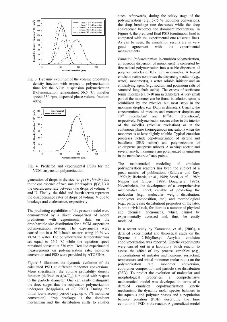
Fig. 3. Dynamic evolution of the volume probability density function with respect to polymerization time for the VCM suspension polymerization (Polymerization temperature: 56.5 oC, impeller speed: 330 rpm, dispersed phase volume fraction: 40%).

0 100 200 3000

20

40

60

80

100

120 Experimental Simulation

Particle Diameter (µm)

Pro

babi

lity

Den

sity

Func

tion

* 10

4 (µm

-1)

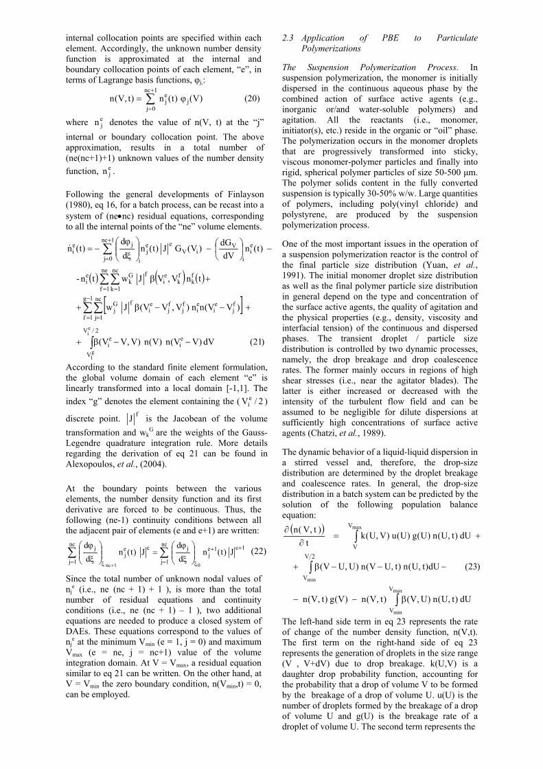
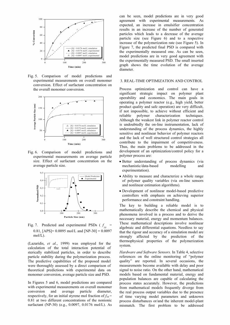
Fig. 4. Predicted and experimental PSDs for the

VCM suspension polymerization

generation of drops in the size range (V , V+dV) due to the coalescence of two smaller droplets. β(V, U) is the coalescence rate between two drops of volume V and U. Finally, the third and fourth terms represent the disappearance rates of drops of volume V due to breakage and coalescence, respectively. The predicting capabilities of the present model were demonstrated by a direct comparison of model predictions with experimental data on the drop/particle size distribution for a VCM suspension polymerization system. The experiments were carried out in a 30 lt batch reactor, using 40 % v/v VCM in water. The polymerization temperature was set equal to 56.5 oC while the agitation speed remained constant at 330 rpm. Detailed experimental measurements on polymerization rate, monomer conversion and PSD were provided by ATOFINA. Figure 3 illustrates the dynamic evolution of the calculated PSD at different monomer conversions. More specifically, the volume probability density function (defined as dv

3n/Vtot) is plotted with respect to the particle diameter. One can easily distinguish the three stages that the suspension polymerization undergoes (Maggioris, et al., 2000). During the initial low-viscosity period (e.g., up to 5% monomer conversion), drop breakage is the dominant mechanism and the distribution shifts to smaller

sizes. Afterwards, during the sticky stage of the polymerization (e.g., 5-75 % monomer conversion), the drop breakage rate decreases while the drop coalescence becomes the dominant mechanism. In Figure 4, the predicted final PSD (continuous line) is compared with the experimental one (discrete line). As can be seen, the simulation results are in very good agreement with the experimental measurements. Emulsion Polymerization. In emulsion polymerization, an aqueous dispersion of monomer(s) is converted by free-radical polymerization into a stable dispersion of polymer particles of 0.1-1 µm in diameter. A typical emulsion recipe comprises the dispersing medium (e.g., water), monomer(s), a water soluble initiator and an emulsifying agent (e.g., sodium and potassium salts of saturated long-chain acids). The excess of surfactant forms micelles (ca. 5-10 nm in diameter). A very small part of the monomer can be found in solution, some is solubilized by the micelles but most stays in the monomer droplets (ca. l0µm in diameter). Usually, the concentrations of micelles and monomer droplets are 1018 micelles/cm3 and 1010-1011 droplets/cm3, respectively. Polymerization occurs either in the interior of the micelles (micellar nucleation) or in the continuous phase (homogeneous nucleation) when the monomer is at least slightly soluble. Typical emulsion processes include copolymerization of styrene and butadiene (SBR rubber) and polymerization of chloroprene (neoprene rubber). Also vinyl acetate and several acrylic monomers are polymerized in emulsion in the manufacture of latex paints. The mathematical modeling of emulsion polymerization reactors has been the subject of a great number of publications (Saldivar and Ray, 1997a,b; Richards, et al., 1989; Storti, et al., 1989; Napper and Gilbert, 1989; Dougherty, 1986). Nevertheless, the development of a comprehensive mathematical model, capable of predicting the molecular (e.g., molecular weight distribution, copolymer composition, etc.) and morphological (e.g., particle size distribution) properties of the latex is not a trivial task, for there is a number of physical and chemical phenomena, which cannot be experimentally assessed and, thus, be easily modelled. In a recent study by Kammona, et al., (2003), a detailed experimental and theoretical study on the Styrene / 2-Ethylhexyl Acrylate emulsion copolymerization was reported. Kinetic experiments were carried out in a laboratory batch reactor to assess the effect of key process variables (e.g., concentrations of initiator and nonionic surfactant, temperature and initial monomer molar ratio) on the polymerization rate, monomer conversion, copolymer composition and particle size distribution (PSD). To predict the evolution of molecular and morphological properties, a comprehensive mathematical model was developed in terms of a detailed emulsion copolymerization kinetic mechanism, the dynamic molar species balances in the aqueous and polymer phases and a population balance equation (PBE) describing the time evolution of PSD in the reactor. A generalized model

0 100 200 3000

20

40

60

80

100

[S] = 0.0176 mol/L simulation [S] = 0.0176 mol/L experimental [S] = 0.0097 mol/L simulation [S] = 0.0097 mol/L experimental

% C

onve

rsio

n

Time (min)

Fig. 5. Comparison of model predictions and experimental measurements on overall monomer conversion. Effect of surfactant concentration on the overall monomer conversion.

0 100 200 300

50

100

150

200

[S] = 0.0176 mol/L simulation [S] = 0.0176 mol/L experimental [S] = 0.0097 mol/L simulation [S] = 0.0097 mol/L experimental

Ave

rage

Par

ticle

Siz

e (n

m)

Time (min)

Fig. 6. Comparison of model predictions and

experimental measurements on average particle size. Effect of surfactant concentration on the average particle size.

0 100 200 3000,0

0,1

0,2

0,3

0,4

0,5

0 100 200 30020

40

60

80

100

120

140

160

180

200

220

240

Part

icle

dia

met

er (n

m)

Time(min)

Model Prediction Experimental

Nor

mal

ized

PSD

Particle Size (nm)

Fig. 7. Predicted and experimental PSDs ( f

10 = 0.81, [APS]= 0.0095 mol/L and [NP-30] = 0.0097 mol/L).

(Lazaridis, et al., 1999) was employed for the calculation of the total interaction potential of sterically stabilized particles, in order to describe particle stability during the polymerization process. The predictive capabilities of the proposed model were thoroughly assessed by a direct comparison of theoretical predictions with experimental data on monomer conversion, average particle size and PSD. In Figures 5 and 6, model predictions are compared with experimental measurements on overall monomer conversion and average particle diameter, respectively, for an initial styrene mol fraction of f10 = 0.81 at two different concentrations of the nonionic surfactant (NP-30) (e.g., 0.0097, 0.0176 mol/L). As

can be seen, model predictions are in very good agreement with experimental measurements. As expected, an increase in emulsifier concentration results in an increase of the number of generated particles which leads to a decrease of the average particle size (see Figure 6) and to a respective increase of the polymerization rate (see Figure 5). In Figure 7, the predicted final PSD is compared with the experimentally measured one. As can be seen, model predictions are in very good agreement with the experimentally measured PSD. The small inserted graph shows the time evolution of the average diameter. 3. REAL-TIME OPTIMIZATION AND CONTROL

Process optimization and control can have a significant strategic impact on polymer plant operability and economics. The main goals in operating a polymer reactor (e.g., high yield, better product quality and safe operation) are very difficult, if not impossible, to achieve without efficient and reliable polymer characterization techniques. Although the weakest link in polymer reactor control is undoubtedly the on-line instrumentation, lack of understanding of the process dynamics, the highly sensitive and nonlinear behavior of polymer reactors and the lack of well structured control strategies all contribute to the impairment of competitiveness. Thus, the main problems to be addressed in the development of an optimization/control policy for a polymer process are: ••

••

Better understanding of process dynamics (via mechanistic/data-based modelling and experimentation).

••

Ability to measure and characterize a whole range of polymer quality variables (via on-line sensors and nonlinear estimation algorithms). Development of nonlinear model-based predictive controllers with emphasis on achieving superior performance and constraint handling.

The key to building a reliable model is to mathematically describe the chemical and physical phenomena involved in a process and to derive the necessary material, energy and momentum balances. These mathematical descriptions involve nonlinear algebraic and differential equations. Needless to say that the rigour and accuracy of a simulation model are strongly affected by the prediction of the thermophysical properties of the polymerization system.

Hardware and Software Sensors. In Table 4, selective references on the online monitoring of “polymer quality” are reported. In several occasions, the measurements become available with delay and poor signal to noise ratio. On the other hand, mathematical models based on fundamental material, energy and population balances are capable of calculating the process states accurately. However, the predictions from mathematical models frequently diverge from the real process output variables due to the presence of time varying model parameters and unknown process disturbances or/and the inherent model-plant mismatch. The first problem to be addressed

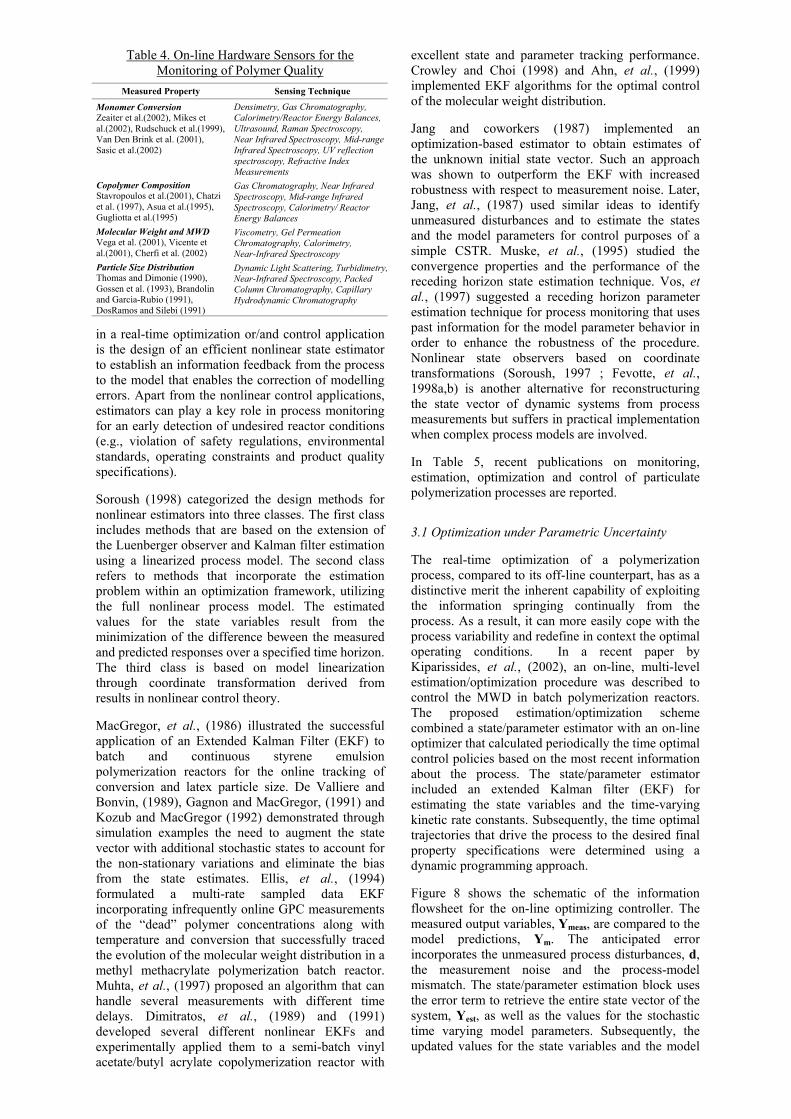
Table 4. On-line Hardware Sensors for the Monitoring of Polymer Quality

in a real-time optimization or/and control application is the design of an efficient nonlinear state estimator to establish an information feedback from the process to the model that enables the correction of modelling errors. Apart from the nonlinear control applications, estimators can play a key role in process monitoring for an early detection of undesired reactor conditions (e.g., violation of safety regulations, environmental standards, operating constraints and product quality specifications). Soroush (1998) categorized the design methods for nonlinear estimators into three classes. The first class includes methods that are based on the extension of the Luenberger observer and Kalman filter estimation using a linearized process model. The second class refers to methods that incorporate the estimation problem within an optimization framework, utilizing the full nonlinear process model. The estimated values for the state variables result from the minimization of the difference beween the measured and predicted responses over a specified time horizon. The third class is based on model linearization through coordinate transformation derived from results in nonlinear control theory. MacGregor, et al., (1986) illustrated the successful application of an Extended Kalman Filter (EKF) to batch and continuous styrene emulsion polymerization reactors for the online tracking of conversion and latex particle size. De Valliere and Bonvin, (1989), Gagnon and MacGregor, (1991) and Kozub and MacGregor (1992) demonstrated through simulation examples the need to augment the state vector with additional stochastic states to account for the non-stationary variations and eliminate the bias from the state estimates. Ellis, et al., (1994) formulated a multi-rate sampled data EKF incorporating infrequently online GPC measurements of the “dead” polymer concentrations along with temperature and conversion that successfully traced the evolution of the molecular weight distribution in a methyl methacrylate polymerization batch reactor. Muhta, et al., (1997) proposed an algorithm that can handle several measurements with different time delays. Dimitratos, et al., (1989) and (1991) developed several different nonlinear EKFs and experimentally applied them to a semi-batch vinyl acetate/butyl acrylate copolymerization reactor with

excellent state and parameter tracking performance. Crowley and Choi (1998) and Ahn, et al., (1999) implemented EKF algorithms for the optimal control of the molecular weight distribution.

Measured Property Sensing Technique

Monomer Conversion Zeaiter et al.(2002), Mikes et al.(2002), Rudschuck et al.(1999), Van Den Brink et al. (2001), Sasic et al.(2002)

Densimetry, Gas Chromatography, Calorimetry/Reactor Energy Balances, Ultrasound, Raman Spectroscopy, Near Infrared Spectroscopy, Mid-range Infrared Spectroscopy, UV reflection spectroscopy, Refractive Index Measurements

Copolymer Composition Stavropoulos et al.(2001), Chatzi et al. (1997), Asua et al.(1995), Gugliotta et al.(1995)

Gas Chromatography, Near Infrared Spectroscopy, Mid-range Infrared Spectroscopy, Calorimetry/ Reactor Energy Balances

Molecular Weight and MWD Vega et al. (2001), Vicente et al.(2001), Cherfi et al. (2002)

Viscometry, Gel Permeation Chromatography, Calorimetry, Near-Infrared Spectroscopy

Particle Size Distribution Thomas and Dimonie (1990), Gossen et al. (1993), Brandolin and Garcia-Rubio (1991), DosRamos and Silebi (1991)

Dynamic Light Scattering, Turbidimetry,Near-Infrared Spectroscopy, Packed Column Chromatography, Capillary Hydrodynamic Chromatography

Jang and coworkers (1987) implemented an optimization-based estimator to obtain estimates of the unknown initial state vector. Such an approach was shown to outperform the EKF with increased robustness with respect to measurement noise. Later, Jang, et al., (1987) used similar ideas to identify unmeasured disturbances and to estimate the states and the model parameters for control purposes of a simple CSTR. Muske, et al., (1995) studied the convergence properties and the performance of the receding horizon state estimation technique. Vos, et al., (1997) suggested a receding horizon parameter estimation technique for process monitoring that uses past information for the model parameter behavior in order to enhance the robustness of the procedure. Nonlinear state observers based on coordinate transformations (Soroush, 1997 ; Fevotte, et al., 1998a,b) is another alternative for reconstructuring the state vector of dynamic systems from process measurements but suffers in practical implementation when complex process models are involved. In Table 5, recent publications on monitoring, estimation, optimization and control of particulate polymerization processes are reported. 3.1 Optimization under Parametric Uncertainty The real-time optimization of a polymerization process, compared to its off-line counterpart, has as a distinctive merit the inherent capability of exploiting the information springing continually from the process. As a result, it can more easily cope with the process variability and redefine in context the optimal operating conditions. In a recent paper by Kiparissides, et al., (2002), an on-line, multi-level estimation/optimization procedure was described to control the MWD in batch polymerization reactors. The proposed estimation/optimization scheme combined a state/parameter estimator with an on-line optimizer that calculated periodically the time optimal control policies based on the most recent information about the process. The state/parameter estimator included an extended Kalman filter (EKF) for estimating the state variables and the time-varying kinetic rate constants. Subsequently, the time optimal trajectories that drive the process to the desired final property specifications were determined using a dynamic programming approach. Figure 8 shows the schematic of the information flowsheet for the on-line optimizing controller. The measured output variables, Ymeas, are compared to the model predictions, Ym. The anticipated error incorporates the unmeasured process disturbances, d, the measurement noise and the process-model mismatch. The state/parameter estimation block uses the error term to retrieve the entire state vector of the system, Yest, as well as the values for the stochastic time varying model parameters. Subsequently, the updated values for the state variables and the model

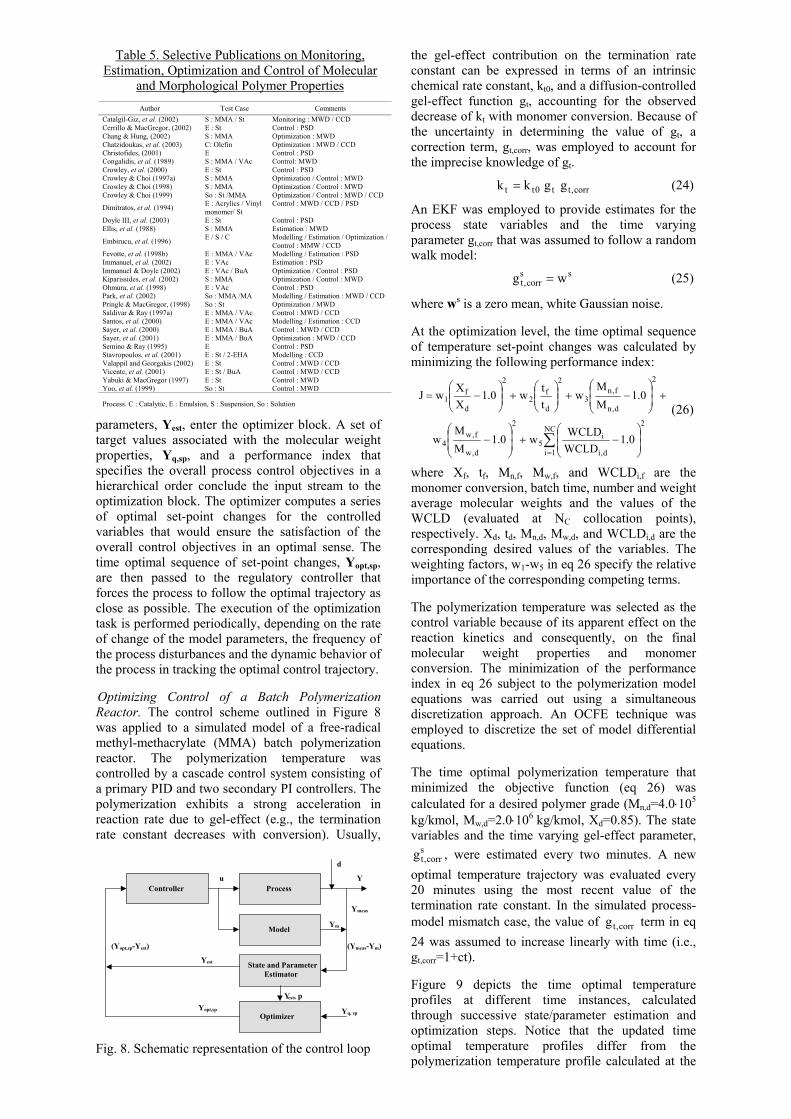
Table 5. Selective Publications on Monitoring, Estimation, Optimization and Control of Molecular

and Morphological Polymer Properties

parameters, Yest, enter the optimizer block. A set of target values associated with the molecular weight properties, Yq,sp, and a performance index that specifies the overall process control objectives in a hierarchical order conclude the input stream to the optimization block. The optimizer computes a series of optimal set-point changes for the controlled variables that would ensure the satisfaction of the overall control objectives in an optimal sense. The time optimal sequence of set-point changes, Yopt,sp, are then passed to the regulatory controller that forces the process to follow the optimal trajectory as close as possible. The execution of the optimization task is performed periodically, depending on the rate of change of the model parameters, the frequency of the process disturbances and the dynamic behavior of the process in tracking the optimal control trajectory. Optimizing Control of a Batch Polymerization Reactor. The control scheme outlined in Figure 8 was applied to a simulated model of a free-radical methyl-methacrylate (MMA) batch polymerization reactor. The polymerization temperature was controlled by a cascade control system consisting of a primary PID and two secondary PI controllers. The polymerization exhibits a strong acceleration in reaction rate due to gel-effect (e.g., the termination rate constant decreases with conversion). Usually,

Controller Process

State and ParameterEstimator

Optimizer

Model

Y

Ymeas

(Yopt,sp-Yest)

Yest

u

Yq, sp

Yest, p

Ym

Yopt,sp

d

(Ymeas-Ym)

Fig. 8. Schematic representation of the control loop

the gel-effect contribution on the termination rate constant can be expressed in terms of an intrinsic chemical rate constant, kt0, and a diffusion-controlled gel-effect function gt, accounting for the observed decrease of kt with monomer conversion. Because of the uncertainty in determining the value of gt, a correction term, gt,corr, was employed to account for the imprecise knowledge of gt.

Author Test Case Comments Catalgil-Giz, et al. (2002) S : MMA / St Monitoring : MWD / CCD Cerrillo & MacGregor, (2002) E : St Control : PSD Chang & Hung, (2002) S : MMA Optimization : MWD Chatzidoukas, et al. (2003) C: Olefin Optimization : MWD / CCD Christofides, (2001) E Control : PSD Congalidis, et al. (1989) S : MMA / VAc Control: MWD Crowley, et al. (2000) E : St Control : PSD Crowley & Choi (1997a) S : MMA Optimization / Control : MWD Crowley & Choi (1998) S : MMA Optimization / Control : MWD Crowley & Choi (1999) So : St /MMA Optimization / Control : MWD / CCD

Dimitratos, et al. (1994) E : Acrylics / Vinyl monomer/ St

Control : MWD / CCD / PSD

Doyle III, et al. (2003) E : St Control : PSD Ellis, et al. (1988) S : MMA Estimation : MWD

Embirucu, et al. (1996) E / S / C Modelling / Estimation / Optimization / Control : MMW / CCD

Fevotte, et al. (1998b) E : MMA / VAc Modelling / Estimation : PSD Immanuel, et al. (2002) E : VAc Estimation : PSD Immanuel & Doyle (2002) E : VAc / BuA Optimization / Control : PSD Kiparissides, et al. (2002) S : MMA Optimization / Control : MWD Ohmura, et al. (1998) E : VAc Control : PSD Park, et al. (2002) So : MMA /MA Modelling / Estimation : MWD / CCD Pringle & MacGregor, (1998) So : St Optimization / MWD Saldivar & Ray (1997a) E : MMA / VAc Control : MWD / CCD Santos, et al. (2000) E : MMA / VAc Modelling / Estimation : CCD Sayer, et al. (2000) E : MMA / BuA Control : MWD / CCD Sayer, et al. (2001) E : MMA / BuA Optimization : MWD / CCD Semino & Ray (1995) E Control : PSD Stavropoulos, et al. (2001) E : St / 2-EHA Modelling : CCD Valappil and Georgakis (2002) E : St Control : MWD / CCD Vicente, et al. (2001) E : St / BuA Control : MWD / CCD Yabuki & MacGregor (1997) E : St Control : MWD Yoo, et al. (1999) So : St Control : MWD Process. C : Catalytic, E : Emulsion, S : Suspension, So : Solution

(24) corr,tt0tt ggkk =

An EKF was employed to provide estimates for the process state variables and the time varying parameter gt,corr that was assumed to follow a random walk model:

(25) sscorr,t wg =

where ws is a zero mean, white Gaussian noise. At the optimization level, the time optimal sequence of temperature set-point changes was calculated by minimizing the following performance index:

2

NC

1i d,i

i5

2

d,w

f,w4

2

d,n

f,n3

2

d

f2

2

d

f1

0.1WCLDWCLDw0.1

MM

w

0.1MM

wttw0.1

XXwJ

∑=

−+

−

+

−+

+

−=

(26)

where Xf, tf, Mn,f, Mw,f, and WCLDi,f are the monomer conversion, batch time, number and weight average molecular weights and the values of the WCLD (evaluated at NC collocation points), respectively. Xd, td, Mn,d, Mw,d, and WCLDi,d are the corresponding desired values of the variables. The weighting factors, w1-w5 in eq 26 specify the relative importance of the corresponding competing terms. The polymerization temperature was selected as the control variable because of its apparent effect on the reaction kinetics and consequently, on the final molecular weight properties and monomer conversion. The minimization of the performance index in eq 26 subject to the polymerization model equations was carried out using a simultaneous discretization approach. An OCFE technique was employed to discretize the set of model differential equations. The time optimal polymerization temperature that minimized the objective function (eq 26) was calculated for a desired polymer grade (Mn,d=4.0⋅105 kg/kmol, Mw,d=2.0⋅106 kg/kmol, Xd=0.85). The state variables and the time varying gel-effect parameter,

, were estimated every two minutes. A new optimal temperature trajectory was evaluated every 20 minutes using the most recent value of the termination rate constant. In the simulated process-model mismatch case, the value of term in eq 24 was assumed to increase linearly with time (i.e., g

scorr,tg

corr,tg

t,corr=1+ct). Figure 9 depicts the time optimal temperature profiles at different time instances, calculated through successive state/parameter estimation and optimization steps. Notice that the updated time optimal temperature profiles differ from the polymerization temperature profile calculated at the

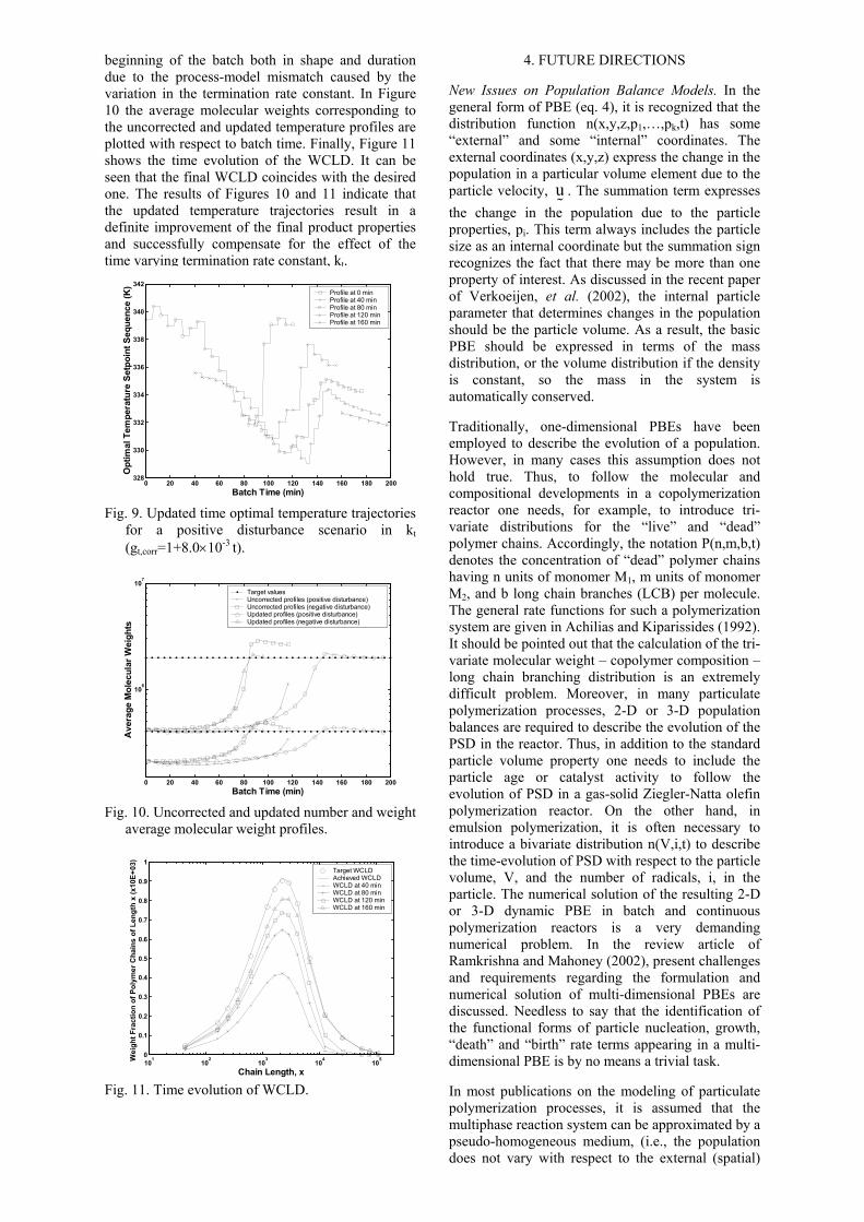
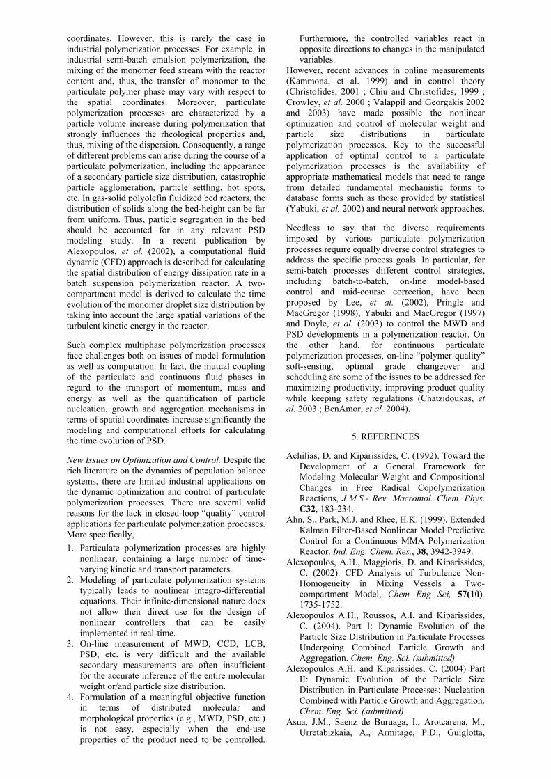
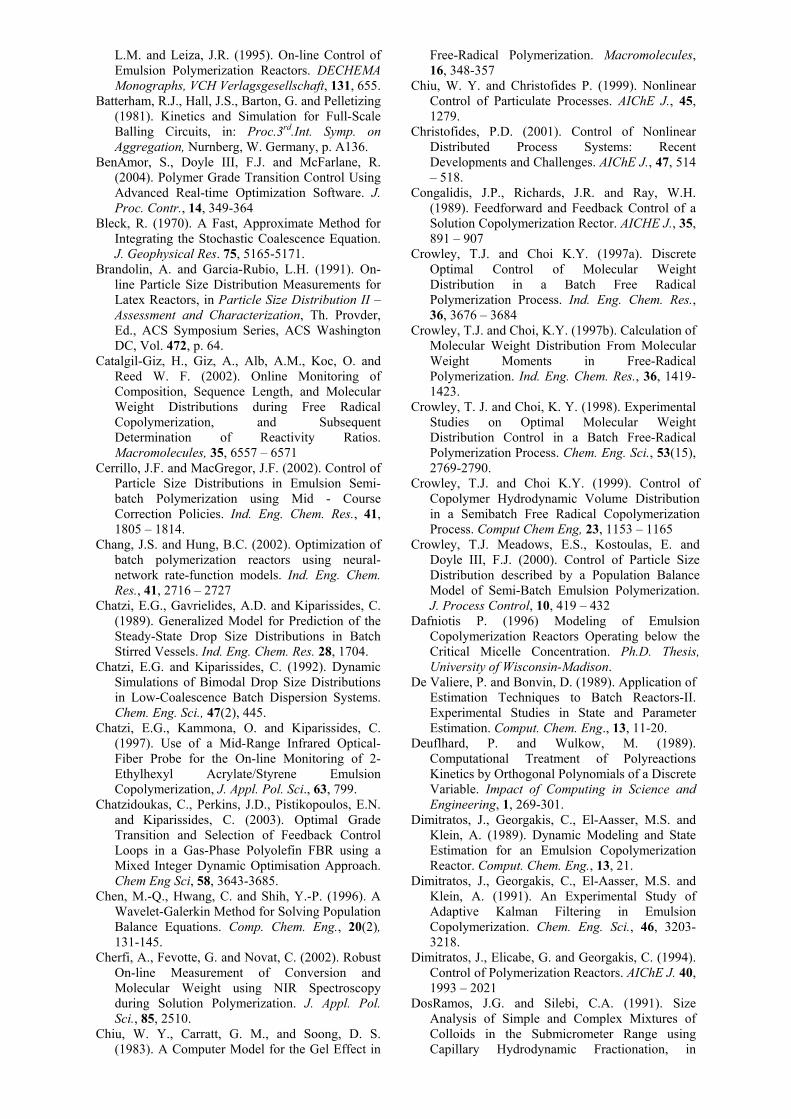
beginning of the batch both in shape and duration due to the process-model mismatch caused by the variation in the termination rate constant. In Figure 10 the average molecular weights corresponding to the uncorrected and updated temperature profiles are plotted with respect to batch time. Finally, Figure 11 shows the time evolution of the WCLD. It can be seen that the final WCLD coincides with the desired one. The results of Figures 10 and 11 indicate that the updated temperature trajectories result in a definite improvement of the final product properties and successfully compensate for the effect of the time varying termination rate constant, kt.

0 20 40 60 80 100 120 140 160 180 200328

330

332

334

336

338

340

342

Batch Time (min)

Opt

imal

Tem

pera

ture

Set

poin

t Seq

uenc

e (K

)

Profile at 0 min Profile at 40 min Profile at 80 min Profile at 120 minProfile at 160 min

Fig. 9. Updated time optimal temperature trajectories

for a positive disturbance scenario in kt (gt,corr=1+8.0×10-3 t).

0 20 40 60 80 100 120 140 160 180 200

106

107

Batch Time (min)

Ave

rage

Mol

ecul

ar W

eigh

ts

Target values Uncorrected profiles (positive disturbance)Uncorrected profiles (negative disturbance)Updated profiles (positive disturbance) Updated profiles (negative disturbance)

Fig. 10. Uncorrected and updated number and weight

average molecular weight profiles.

10

110

210

310

410

50

0.1

0.2

0.3

0.4

0.5

0.6

0.7

0.8

0.9

1

Chain Length, x

Wei

ght F

ract

ion

of P

olym

er C

hain

s of

Len

gth

x (x

10E+

03)

Target WCLD Achieved WCLD WCLD at 40 min WCLD at 80 min WCLD at 120 minWCLD at 160 min

Fig. 11. Time evolution of WCLD.

4. FUTURE DIRECTIONS

New Issues on Population Balance Models. In the general form of PBE (eq. 4), it is recognized that the distribution function n(x,y,z,p1,…,pk,t) has some “external” and some “internal” coordinates. The external coordinates (x,y,z) express the change in the population in a particular volume element due to the particle velocity, . The summation term expresses the change in the population due to the particle properties, p

u

i. This term always includes the particle size as an internal coordinate but the summation sign recognizes the fact that there may be more than one property of interest. As discussed in the recent paper of Verkoeijen, et al. (2002), the internal particle parameter that determines changes in the population should be the particle volume. As a result, the basic PBE should be expressed in terms of the mass distribution, or the volume distribution if the density is constant, so the mass in the system is automatically conserved. Traditionally, one-dimensional PBEs have been employed to describe the evolution of a population. However, in many cases this assumption does not hold true. Thus, to follow the molecular and compositional developments in a copolymerization reactor one needs, for example, to introduce tri-variate distributions for the “live” and “dead” polymer chains. Accordingly, the notation P(n,m,b,t) denotes the concentration of “dead” polymer chains having n units of monomer M1, m units of monomer M2, and b long chain branches (LCB) per molecule. The general rate functions for such a polymerization system are given in Achilias and Kiparissides (1992). It should be pointed out that the calculation of the tri-variate molecular weight – copolymer composition – long chain branching distribution is an extremely difficult problem. Moreover, in many particulate polymerization processes, 2-D or 3-D population balances are required to describe the evolution of the PSD in the reactor. Thus, in addition to the standard particle volume property one needs to include the particle age or catalyst activity to follow the evolution of PSD in a gas-solid Ziegler-Natta olefin polymerization reactor. On the other hand, in emulsion polymerization, it is often necessary to introduce a bivariate distribution n(V,i,t) to describe the time-evolution of PSD with respect to the particle volume, V, and the number of radicals, i, in the particle. The numerical solution of the resulting 2-D or 3-D dynamic PBE in batch and continuous polymerization reactors is a very demanding numerical problem. In the review article of Ramkrishna and Mahoney (2002), present challenges and requirements regarding the formulation and numerical solution of multi-dimensional PBEs are discussed. Needless to say that the identification of the functional forms of particle nucleation, growth, “death” and “birth” rate terms appearing in a multi-dimensional PBE is by no means a trivial task. In most publications on the modeling of particulate polymerization processes, it is assumed that the multiphase reaction system can be approximated by a pseudo-homogeneous medium, (i.e., the population does not vary with respect to the external (spatial)

coordinates. However, this is rarely the case in industrial polymerization processes. For example, in industrial semi-batch emulsion polymerization, the mixing of the monomer feed stream with the reactor content and, thus, the transfer of monomer to the particulate polymer phase may vary with respect to the spatial coordinates. Moreover, particulate polymerization processes are characterized by a particle volume increase during polymerization that strongly influences the rheological properties and, thus, mixing of the dispersion. Consequently, a range of different problems can arise during the course of a particulate polymerization, including the appearance of a secondary particle size distribution, catastrophic particle agglomeration, particle settling, hot spots, etc. In gas-solid polyolefin fluidized bed reactors, the distribution of solids along the bed-height can be far from uniform. Thus, particle segregation in the bed should be accounted for in any relevant PSD modeling study. In a recent publication by Alexopoulos, et al. (2002), a computational fluid dynamic (CFD) approach is described for calculating the spatial distribution of energy dissipation rate in a batch suspension polymerization reactor. A two-compartment model is derived to calculate the time evolution of the monomer droplet size distribution by taking into account the large spatial variations of the turbulent kinetic energy in the reactor. Such complex multiphase polymerization processes face challenges both on issues of model formulation as well as computation. In fact, the mutual coupling of the particulate and continuous fluid phases in regard to the transport of momentum, mass and energy as well as the quantification of particle nucleation, growth and aggregation mechanisms in terms of spatial coordinates increase significantly the modeling and computational efforts for calculating the time evolution of PSD. New Issues on Optimization and Control. Despite the rich literature on the dynamics of population balance systems, there are limited industrial applications on the dynamic optimization and control of particulate polymerization processes. There are several valid reasons for the lack in closed-loop “quality” control applications for particulate polymerization processes. More specifically, 1. Particulate polymerization processes are highly

nonlinear, containing a large number of time-varying kinetic and transport parameters.

2. Modeling of particulate polymerization systems typically leads to nonlinear integro-differential equations. Their infinite-dimensional nature does not allow their direct use for the design of nonlinear controllers that can be easily implemented in real-time.

3. On-line measurement of MWD, CCD, LCB, PSD, etc. is very difficult and the available secondary measurements are often insufficient for the accurate inference of the entire molecular weight or/and particle size distribution.

4. Formulation of a meaningful objective function in terms of distributed molecular and morphological properties (e.g., MWD, PSD, etc.) is not easy, especially when the end-use properties of the product need to be controlled.

Furthermore, the controlled variables react in opposite directions to changes in the manipulated variables.

However, recent advances in online measurements (Kammona, et al. 1999) and in control theory (Christofides, 2001 ; Chiu and Christofides, 1999 ; Crowley, et al. 2000 ; Valappil and Georgakis 2002 and 2003) have made possible the nonlinear optimization and control of molecular weight and particle size distributions in particulate polymerization processes. Key to the successful application of optimal control to a particulate polymerization processes is the availability of appropriate mathematical models that need to range from detailed fundamental mechanistic forms to database forms such as those provided by statistical (Yabuki, et al. 2002) and neural network approaches. Needless to say that the diverse requirements imposed by various particulate polymerization processes require equally diverse control strategies to address the specific process goals. In particular, for semi-batch processes different control strategies, including batch-to-batch, on-line model-based control and mid-course correction, have been proposed by Lee, et al. (2002), Pringle and MacGregor (1998), Yabuki and MacGregor (1997) and Doyle, et al. (2003) to control the MWD and PSD developments in a polymerization reactor. On the other hand, for continuous particulate polymerization processes, on-line “polymer quality” soft-sensing, optimal grade changeover and scheduling are some of the issues to be addressed for maximizing productivity, improving product quality while keeping safety regulations (Chatzidoukas, et al. 2003 ; BenAmor, et al. 2004).

5. REFERENCES

Achilias, D. and Kiparissides, C. (1992). Toward the

Development of a General Framework for Modeling Molecular Weight and Compositional Changes in Free Radical Copolymerization Reactions, J.M.S.- Rev. Macromol. Chem. Phys. C32, 183-234.

Ahn, S., Park, M.J. and Rhee, H.K. (1999). Extended Kalman Filter-Based Nonlinear Model Predictive Control for a Continuous MMA Polymerization Reactor. Ind. Eng. Chem. Res., 38, 3942-3949.

Alexopoulos, A.H., Maggioris, D. and Kiparissides, C. (2002). CFD Analysis of Turbulence Non-Homogeneity in Mixing Vessels a Two-compartment Model, Chem Eng Sci, 57(10), 1735-1752.

Alexopoulos A.H., Roussos, A.I. and Kiparissides, C. (2004). Part I: Dynamic Evolution of the Particle Size Distribution in Particulate Processes Undergoing Combined Particle Growth and Aggregation. Chem. Eng. Sci. (submitted)

Alexopoulos A.H. and Kiparissides, C. (2004) Part II: Dynamic Evolution of the Particle Size Distribution in Particulate Processes: Nucleation Combined with Particle Growth and Aggregation. Chem. Eng. Sci. (submitted)

Asua, J.M., Saenz de Buruaga, I., Arotcarena, M., Urretabizkaia, A., Armitage, P.D., Guiglotta,

L.M. and Leiza, J.R. (1995). On-line Control of Emulsion Polymerization Reactors. DECHEMA Monographs, VCH Verlagsgesellschaft, 131, 655.

Batterham, R.J., Hall, J.S., Barton, G. and Pelletizing (1981). Kinetics and Simulation for Full-Scale Balling Circuits, in: Proc.3rd.Int. Symp. on Aggregation, Nurnberg, W. Germany, p. A136.

BenAmor, S., Doyle III, F.J. and McFarlane, R. (2004). Polymer Grade Transition Control Using Advanced Real-time Optimization Software. J. Proc. Contr., 14, 349-364

Bleck, R. (1970). A Fast, Approximate Method for Integrating the Stochastic Coalescence Equation. J. Geophysical Res. 75, 5165-5171.

Brandolin, A. and Garcia-Rubio, L.H. (1991). On-line Particle Size Distribution Measurements for Latex Reactors, in Particle Size Distribution II – Assessment and Characterization, Th. Provder, Ed., ACS Symposium Series, ACS Washington DC, Vol. 472, p. 64.

Catalgil-Giz, H., Giz, A., Alb, A.M., Koc, O. and Reed W. F. (2002). Online Monitoring of Composition, Sequence Length, and Molecular Weight Distributions during Free Radical Copolymerization, and Subsequent Determination of Reactivity Ratios. Macromolecules, 35, 6557 – 6571

Cerrillo, J.F. and MacGregor, J.F. (2002). Control of Particle Size Distributions in Emulsion Semi-batch Polymerization using Mid - Course Correction Policies. Ind. Eng. Chem. Res., 41, 1805 – 1814.

Chang, J.S. and Hung, B.C. (2002). Optimization of batch polymerization reactors using neural-network rate-function models. Ind. Eng. Chem. Res., 41, 2716 – 2727

Chatzi, E.G., Gavrielides, A.D. and Kiparissides, C. (1989). Generalized Model for Prediction of the Steady-State Drop Size Distributions in Batch Stirred Vessels. Ind. Eng. Chem. Res. 28, 1704.

Chatzi, E.G. and Kiparissides, C. (1992). Dynamic Simulations of Bimodal Drop Size Distributions in Low-Coalescence Batch Dispersion Systems. Chem. Eng. Sci., 47(2), 445.

Chatzi, E.G., Kammona, O. and Kiparissides, C. (1997). Use of a Mid-Range Infrared Optical-Fiber Probe for the On-line Monitoring of 2-Ethylhexyl Acrylate/Styrene Emulsion Copolymerization, J. Appl. Pol. Sci., 63, 799.

Chatzidoukas, C., Perkins, J.D., Pistikopoulos, E.N. and Kiparissides, C. (2003). Optimal Grade Transition and Selection of Feedback Control Loops in a Gas-Phase Polyolefin FBR using a Mixed Integer Dynamic Optimisation Approach. Chem Eng Sci, 58, 3643-3685.

Chen, M.-Q., Hwang, C. and Shih, Y.-P. (1996). A Wavelet-Galerkin Method for Solving Population Balance Equations. Comp. Chem. Eng., 20(2), 131-145.

Cherfi, A., Fevotte, G. and Novat, C. (2002). Robust On-line Measurement of Conversion and Molecular Weight using NIR Spectroscopy during Solution Polymerization. J. Appl. Pol. Sci., 85, 2510.

Chiu, W. Y., Carratt, G. M., and Soong, D. S. (1983). A Computer Model for the Gel Effect in

Free-Radical Polymerization. Macromolecules, 16, 348-357

Chiu, W. Y. and Christofides P. (1999). Nonlinear Control of Particulate Processes. AIChE J., 45, 1279.

Christofides, P.D. (2001). Control of Nonlinear Distributed Process Systems: Recent Developments and Challenges. AIChE J., 47, 514 – 518.

Congalidis, J.P., Richards, J.R. and Ray, W.H. (1989). Feedforward and Feedback Control of a Solution Copolymerization Rector. AICHE J., 35, 891 – 907

Crowley, T.J. and Choi K.Y. (1997a). Discrete Optimal Control of Molecular Weight Distribution in a Batch Free Radical Polymerization Process. Ind. Eng. Chem. Res., 36, 3676 – 3684

Crowley, T.J. and Choi, K.Y. (1997b). Calculation of Molecular Weight Distribution From Molecular Weight Moments in Free-Radical Polymerization. Ind. Eng. Chem. Res., 36, 1419-1423.

Crowley, T. J. and Choi, K. Y. (1998). Experimental Studies on Optimal Molecular Weight Distribution Control in a Batch Free-Radical Polymerization Process. Chem. Eng. Sci., 53(15), 2769-2790.

Crowley, T.J. and Choi K.Y. (1999). Control of Copolymer Hydrodynamic Volume Distribution in a Semibatch Free Radical Copolymerization Process. Comput Chem Eng, 23, 1153 – 1165

Crowley, T.J. Meadows, E.S., Kostoulas, E. and Doyle III, F.J. (2000). Control of Particle Size Distribution described by a Population Balance Model of Semi-Batch Emulsion Polymerization. J. Process Control, 10, 419 – 432

Dafniotis P. (1996) Modeling of Emulsion Copolymerization Reactors Operating below the Critical Micelle Concentration. Ph.D. Thesis, University of Wisconsin-Madison.

De Valiere, P. and Bonvin, D. (1989). Application of Estimation Techniques to Batch Reactors-II. Experimental Studies in State and Parameter Estimation. Comput. Chem. Eng., 13, 11-20.

Deuflhard, P. and Wulkow, M. (1989). Computational Treatment of Polyreactions Kinetics by Orthogonal Polynomials of a Discrete Variable. Impact of Computing in Science and Engineering, 1, 269-301.

Dimitratos, J., Georgakis, C., El-Aasser, M.S. and Klein, A. (1989). Dynamic Modeling and State Estimation for an Emulsion Copolymerization Reactor. Comput. Chem. Eng., 13, 21.

Dimitratos, J., Georgakis, C., El-Aasser, M.S. and Klein, A. (1991). An Experimental Study of Adaptive Kalman Filtering in Emulsion Copolymerization. Chem. Eng. Sci., 46, 3203-3218.

Dimitratos, J., Elicabe, G. and Georgakis, C. (1994). Control of Polymerization Reactors. AIChE J. 40, 1993 – 2021

DosRamos, J.G. and Silebi, C.A. (1991). Size Analysis of Simple and Complex Mixtures of Colloids in the Submicrometer Range using Capillary Hydrodynamic Fractionation, in

Particle Size Distribution II – Assessment and Characterization, Th. Provder, Ed., ACS Symposium Series, ACS Washington DC, Vol. 472, p. 292.

Dougherty, E.P., (1986). The SCOPE Dynamic Model for Emulsion Polymerization I. Theory. J. Appl. Pol. Sci., 32(1), 3051.

Doyle III, F.J., Harrison, C.A. and Crowley, T.J. (2003). Hybrid Model-Based approach to Batch-to-Batch Control of Particle Size Distribution in Emulsion Polymerization. Comp. Chem. Eng., 27, 1153 – 1163

Ellis, M.F., Taylor, T.W., Gonzalez, V. and Jensen K. (1988). Estimation of the Molecular Weight Distribution in Batch Polymerization. AIChE J., 34, 1341 – 1353

Ellis, M.F., Taylor, T.W. and Jensen K.F. (1994). Online Molecular Weight Distribution Estimation and Control in Batch Polymerization. AIChE J., 40, 445-462.

Embirucu, M., Lima, E.L. and Pinto, J.C. (1996). A Survey of Advanced Control of Polymerization Reactors. Polymer Engineering Science, 36, 433 – 447

Erasmus, L.D., Eyre, D. and Everson, R.C. (1994). Numerical Treatment of the Population Balance Equation Using a Spline-Galerkin method, Comput Chem Eng, 18(9), 775-783

Fèvotte, G., McKenna, T.F., Othman, S. and Hammouri, H. (1998a). Nonlinear Tracking of Glass Transition Temperatures for Free Radical Emulsion Copolymers. Chem. Eng. Sci., 53, 773-786.

Fèvotte, G., McKenna, T.F., Othman, S. and Santos, A.M. (1998b). A Combined Hardware/Software Sensing approach for On-Line Control of Emulsion Polymerization Process. Comp. Chem. Eng., 22, 443 – 449

Finlayson, B.A. (1980). Nonlinear Analysis in Chemical Engineering. McGraw-Hill, NY, New York

Gagnon, L. and MacGregor, J.F. (1991). State Estimation for Continuous Emulsion Polymerization. Can. J. Chem. Eng., 69, 648-656.

Gelbard, F. and Seinfeld, J.H. (1978). Numerical solution of the dynamical equation for particulate systems, Jf Comput Phys, 28, 357-375

Gelbard, F. and Seinfeld, J.H. (1979). Exact Solution of the General Dynamic Equation for Aerosol Growth by Condensation. J. Colloid Interface Sci., 68(1), 173.

Gelbard, F. and Seinfeld, J.H. (1980). Simulation of Multicomponent Aerosol Dynamics. J. Colloid Interface Sci., 78(2), 485.

Gelbard F., Tambour Y. and Seinfeld J.H. (1980) Sectional Representation for Simulating Aerosol Dynamics. J. Colloid Interface Science, 76(2), 541-556

Gossen, P.D., MacGregor, J.F. and Pelton, R.H. (1993). Composition and Particle Diameter for Styrene/Methyl Methacrylate Copolymer Latex using UV and NIR Spectroscopy. Appl. Spectr., 47(11), 928.

Guiglotta, L.M., Arotcarena, M., Leiza, J.R. and Asua, J.M. (1995). Estimation of Conversion and copolymer Composition in Semicontinuous

Emulsion Polymerization using Calorimetric Data. Polymer, 36(10), 2019.

Hidy, G.M. (1965). On the Theory of the Coagulation of Noninteracting Particles in Brownian Motion. J. Colloid Sci., 20, 123.

Himmelblau, D.M. and Bischoff, K.B. (1968). Process Analysis and Simulation. Deterministic Systems. John Wiley & Sons, Inc

Hounslow M.J., Ryall, R.L. and Marshall, V.R. (1988). Discretized Population Balance for Nucleation, Growth, and Aggregation. AIChE J., 34(11), 1821-1832.

Hulburt, H.M. and Katz, S. (1964). Some Problems in Particle technology. A Statistical Mechanical Formulation. Chem. Eng. Sci., 19, 555

Iedema, P. D., Wulkow M. and Hoefsloot, C. J. (2000). Modeling Molecular Weight and Degree of Branching Distribution of Low-Density Polyethylene. Macromolecules, 33(19), 7173-7184.

Immanuel, C.D., Cordeiro, C.F., Sundaram, S.S., Meadows, E.S., Crowley, T.J. and Doyle III, F.J. (2002). Modeling of Particle Size Distribution in Emulsion Co-Polymerization: Comparison with Experimental Data and parametric Sensitivity Studies. Comp. Chem. Eng., 26, 1133 – 1152

Immanuel, C.D. and Doyle III, F.J. (2002). Open-Loop Control of Particle Size Distribution in Semibatch Emulsion Copolymerization using a Genetic Algorithm. Chem. Eng. Sci., 57, 4415 – 4427

Jang, S.S., Joseph, B. and Mukai, H. (1987). Control of Constrained Multivariable Nonlinear Process using a Two-Phase Approach. Ind. Eng. Chem. Res., 26, 2106-2114.

Kammona, O., Chatzi, E.G. and Kiparissides, C. (1999). Recent Developments in Hardware Sensors for the On-line Monitoring of Polymerization Reactions. J. Macromol Sci., Rev Macromol Chem Phys, C39(1), 57-134

Kammona, O., Pladis, P., Frantzikinakis, C. and Kiparissides, C. (2003). A Comprehensive Experimental and Theoretical Investigation of the Styrene/2-Ethylhexyl Acrylate Emulsion Copolymerization. Macromol.Chem.Phys., 204, 983-999

Kiparissides, C. (1996). Polymerization reactor modeling: A Review of Recent Developments and Future Directions. Chem. Eng. Sci., 51, 1637

Kiparissides, C., Seferlis, P., Mourikas, G. and Morris, A.J. (2002). Online Optimizing Control of Molecular Weight Properties in Batch Free-Radical Polymerization Reactors. Ind. Eng. Chem. Res., 41, 6120 – 6131

Kostoglou M. and Karabelas A.J. (1994). Evaluation of Zero Order Methods for Simulating Particle Coagulation. J. Colloid Interface Sci., 163, 420.

Kostoglou M. and Karabelas A.J. (1995). Evaluation of Numerical Methods for Simulating an Evolving Particle Size Distribution in Growth Processes. Chem. Eng. Comm., 136, 177.

Kozub, D.J. and MacGregor, J.F. (1992). State Estimation for Semi-Batch Polymerization Reactors. Chem. Eng. Sci., 47, 1047-1062.

Kumar, S. and Ramkrishna, D. (1996a). On the Solution of Population Balance Equations by

Discretization-I. A Fixed Pivot Technique. Chem. Eng. Sci., 51(8), 1311-1332.

Kumar, S. and Ramkrishna, D. (1996b). On the Solution of Population Balance Equations by Discretization-II. A Moving Pivot Technique. Chem. Eng. Sci., 51(8), 1333-1342.

Kumar, S. and Ramkrishna, D. (1997). On The Solution of Population Balance Equations by Discretization III. Simultaneous Nucleation, Growth and Aggregation. Chem. Eng. Sci., 52, 4659-4679.

Landgrebe, J.D. and Pratsinis, S.E. (1990). A Discrete-Sectional Model for Powder Production by Gas-Phase Chemical reaction and Aerosol Coagulation in the Free-Molecular Regime. J. Colloid Interface Sci., 139(1), 63-86.

Lazaridis, N., Alexopoulos, A.H., Chatzi, E.G. and Kiparissides, C. (1999). Steric Stabilization in Emulsion Polymerization Using Oligomeric Nonionic Surfactants. Chem. Eng. Sci., 54, 3251-3261.

Lee, K., Lee, J.H., Yang, D.R. and Mahoney, A.W. (2002). Integrated Run-to Run and On-line Model-Based Control of Particle Size Distribution for a Semi-Batch Precipitation Reactor, Comp. Chem. Eng., 26, 1117-1131.

Litster, J.D., Smit, D.J. and Hounslow, M.J. (1995). Adjustable Discretized Population Balance for Growth and Aggregation. AIChE J., 41, 591-603.

MacGregor, J.F., Kozub, D.J., Penlidis, A. and Hamielec, A.E. (1986). State Estimation for Polymerization Reactors. IFAC Symp. On Dynamic and Control of Chemical Reactors and Distillation Columns, Bournemouth, UK, Pergamon Press.

Maggioris, D., Goulas, A., Alexopoulos, A.H., Chatzi, E.G. and Kiparissides C. (2000). Prediction of Particle Size Distribution in Suspension Polymerization Reactors: Effect of Turbulence Nonhomogeneity. Chem. Eng. Sci., 55, 4611.

Mahoney, A.W. and Ramkrishna, D. (2002). Efficient Solution of Population Balance Equations with Discontinuities by Finite Elements. Chem Eng Sci, 57, 1107-1119

Marchal P., David, R., Klein, J.P. and Villermaux, J. (1988). Crystallization and Precipitation Engineering-I. An Efficient Method for Solving Population Balance in Crystallization with Agglomeration. Chem. Eng. Sci., 43(1), 59-67.

Mikes, F., Gonzalez-Benito, B., Serrano, B., Bravo, J. and Baselga, J., (2002). Fluorescence Monitoring of Polymerization Reaction. A New Method for Treating Fluorescence Experimental Data. Polymer, 43, 4331.

Muske, K.R., Rawlings, J.B. and Lee, J.H. (1995). Receding Horizon Recursive State Estimation. In R. Berber (ed), Methods of Model Based Process Control, 349-365, Kluwer, Dordrecht.

Mutha, R.K., Cluett, W.R. and Penlidis, A. (1997). A New Multirate-Measurement-Based Estimator: Emulsion Copolymerization Batch Reactor Case Study. Ind. Eng. Chem. Res., 36, 1036-1047.

Napper, D. H and Gilbert, R.G. (1989). Polymerization in Emulsions, in: Comprehensive

Polymer Science, I. Pirma, Eds., Pergamon, Oxford, Vol. IV, p.171.

Nicmanis, M. and Hounslow, M.J. (1996). A Finite Element Analysis of the Steady State Population Balance Equation for Particulate Systems: Aggregation and Growth. Comp. Chem. Eng., 20, S261.

Nicmanis, M. and Hounslow, M.J. (1998). Finite-Element Methods for Steady-State Population Balance Equations. AIChE J., 44, 2258.

Ohmura, N., Kataoka, K., Watanabe, S. and Okubo, M. (1998). Controlling Particle Size by Self-Sustained Oscillations in Continuous Emulsion Polymerization of Vinyl Acetate. Chem. Eng. Sci., 53, 2129 – 2135

Park, M.J., Hur, S.M. and Rhee, H.K. (2002). Online Estimation and Control of Polymer Quality in a Polymerization Reactor. AIChE J., 48, 1013 – 1021

Pilinis C. (1990) Derivation and Numerical Solution of the Species Mass Distribution Equation for Multicomponent Particulate Systems, Atmos. Environ. A, 24 (7), 1923–1928

Pladis, P. and Kiparissides, C. (1998). A Comprehensive Model for the Calculation of Molecular Weight-Long-Chain Branching Distribution in Free-Radical Polymerizations. Chem. Eng. Sci., 53(18), 3315-3333.

Pringle, T.L.C., and MacGregor, J. F. (1998). Optimization of Molecular Weight Distribution using Batch-to-Batch Adjustments. Ind. Eng. Chem. Res., 37, 3660 – 3669

Ramkrishna, D. (1985). The Status of Population Balances. Reviews Chem. Eng., 3(1), 49.

Ramkrishna, D. and Mahoney, A.W. (2002). Population Balance Modeling. Promise for the Future. Chem Eng Sci, 57, 595-606

Richards, J.R., Congalidis, J.P. and Gilbert, R., (1989). Mathematical Modeling of Emulsion Copolymerization Reactors. J. Appl. Pol. Sci., 37, 2727.

Rigopoulos S., and Jones A.G. (2003). Finite-Element Scheme for Solution of the Dynamic Population Balance Equation. AIChE J., 49(5), 1127-1139

Rudschuck, S., Adams, J., Fuhrmann, J., (1999). Online Observation of Emulsion Polymerization by Fluorescence Technique. Nuclear Instruments and Methods in Physics Research B, 151, 341.

Saldivar, E. and Ray, W.H., (1997a). Control of Semicontinuous Emulsion Copolymerization Reactor. AIChE J., 43, 2021 – 2033

Saldivar, E. and Ray, W.H., (1997b). Mathematical Modeling of Emulsion Copolymerization Reactors: Experimental Validation and Application to Complex Systems. Ind. Eng. Chem. Res., 36(4), 1322

Sampson K.J., and Ramkrishna D. (1985) A New Solution to the Brownian Coagulation Equation through the Use of Root-Shifted Problem-Specific Polynomials, J. Coll Int. Sci., 103(1), 245-254.

Santos, A. M., Fevotte, G., Othman, N. and McKenna, T.F. (2000). On-line monitoring of methyl-methacrylate-vinyl acetate emulsion

copolymerization. J. Appl. Polym. Sci., 75, 1667 – 1683

Sandu, A. and Borden, C. (2003). A Framework for the Numerical Treatment of Aerosol Dynamics. Appl. Num. Math., 45, 475-497.

Sasic, S., Ozaki, Y., Olinga, A. and Siesler, H.W., (2002). Comparison of Various Chemometric Evaluation approaches for On-line FT-NIR Transmission and FT-MIR/ATR Spectroscopic Data of Methyl Methacrylate Solution Polymerization. Anal. Chim. Acta, 452, 265.

Sastry K.V.S, and Gaschignard P., ‘Discretization Procedure for the Coalescence of Particulate Processes’, Ind. Eng. Chem. Fundam., 20, 355-361 (1981).Sayer, C., Lima, E.L., Pinto, J.C., Arzamendi, G. and Asua, J.M. (2000). Molecular Weight Distribution in Composition controlled Emulsion Polymerization. J. Appl. Polym. Sci., 38, 1100 – 1109

Sayer, C., Arzamendi, G., Asua, J.M., Lima, E.L. and Pinto, J.C. (2001). Dynamic Optimization of Semicontinuous Emulsion Copolymerization Reactions: Composition and Molecular Weight Distribution. Comp. Chem. Eng., 25, 839 – 849

Semino, D., and Ray, W.H. (1995). Control of Systems described by Population Balance Equations – I. Controllability Analysis. Chem. Eng. Sci., 50, 1805 – 1824

Singh P.N. and Ramkrishna D. (1975). Transient Solution of the Brownian Coagulation Equation by Problem-Specific Polynomials, J. Coll Int. Sci., 53(2), 214-223

Soroush, M. (1997). Nonlinear State-Observer Design with Application to Reactors. Chem. Eng. Sci., 52, 387-404.

Soroush, M. (1998). State and Parameter Estimations and their Applications in Process Control. Comput. Chem. Eng., 23, 229-245.

Stavropoulos, Y., Kammona, O., Chatzi, E.G. and Kiparissides, C. (2001). Multivariate Statistical Analysis of Mid-Infrared Spectra for the Online Monitoring of 2-Ethylhexyl Acrylate / Styrene Emulsion Copolymerization. J. Appl. Polym. Sci., 82, 1776 – 1787

Storti, G., Morbidelli, M. and Carra, S. (1989). Detailed Modeling of Multicomponent Emulsion Polymerization Systems”, in: Computer Applications in Applied Polymer Science II: Automation, Modelling and Simulation, p.379, T. Provder, Eds., ACS Symposium. Series, 404, Washington DC,.

Tobita, H. (1993). Molecular Weight Distribution in Free-Radical Polymerization with Long-Chain Branching. J. Polymer Sci., 31, 1363.

Tobita, H. (1995). Molecular Weight Distribution in Free-Radical Polymerization with Chain-Length-Dependent Bimolecular Termination. 1. Bulk Polymerization. Macromolecules, 28, 5119.

Tobita, H. and Ito K. (1993). On The Calculation of Molecular Weight Distribution from the Moments Using Laguerre Polynomials. Polymer Reaction Eng., 1(3), 407-425.

Thomas, J. and Dimonie, V. (1990). Fiber Optic Dynamic Light Scattering from Concentrated Dispersions. 3: Particle Sizing in Concentrates. Appl. Optics, 29(36), 5332.

Valappil, J. and Georgakis, C. (2002). Nonlinear Model Predictive Control of End-Use Properties in Batch Reactors. AIChE J., 48, 2006 – 2021

Valappil, J. and Georgakis, C. (2003). Accounting for Batch Reactor Uncertainty in the Nonlinear MPC of End-Use Properties. AIChE J., 49, 1178-1192

Van Den Brink, M., Hansen, J.-F., De Peinder, P., Van Herk, A.M. and German, A.L., (2001). Measurement of Partial Conversions During the Solution Copolymerization of Styrene and Butyl Acrylate Using On-line Raman Spectroscopy. J. Appl. Pol. Sci., 79, 426.

Vanni M., (2000). Approximate Population Balance Equations for Aggregation-Breakage Processes. J. Coll Int. Sci., 221, 143-160.

Vega, M.P., Lima, E.L. and Pinto, J.C. (2001). In-line Monitoring of Weight Average Molecular Weight in Solution Polymerizations using Intrinsic Viscosity Measurements. Polymer, 42, 3009.

Verkoeijen, D., Pouw, G.A., Meesters, G.M.H and Scarlett, B. (2002). Population Balances for Particulate Processes – A Volume Approach. Chem. Eng. Sci., 57, 2287-2303

Vicente, M., Leiza, J.R. and Asua, J.M. (2001). Simultaneous Control of Copolymer Composition and MWD in Emulsion Copolymerization. AIChE J., 47, 1594 – 1606

Vos, B.J., Grievink, J., de Jong, P.J. and Verheijen P.J.T. (1997). A Robust Mode-Based Approach for Online Monitoring of Dynamic Process Performance. Paper 194d, Annual AIChE Meeting, Los Angeles.

Wulkow, M. (1992). Adaptive Treatment of Polyreactions in Weighted Sequence Spaces. Impact of Computing in Science and Engineering, 4, 153-193

Yabuki, Y., and MacGregor, J.F. (1997). Product Quality Control in Semibatch Reactor using Midcourse Correction policies. Ind. Eng. Chem. Res., 36, 1268 – 1275

Yabuki, Y., Nagasawa, T. and MacGregor, J.F. (2002). Industrial Experiences with Product Quality in Semi-Batch Processes. Comp. Chem. Eng., 26, 205 – 212

Yoo, K.Y., Jeong, G. and Rhee, H.K. (1999). Molecular Weight distribution Control in a Batch Polymerization Reactor using the On-line Two-Step Method. Ind. Eng. Chem. Res., 38, 4805 – 4814

Yuan, H.G., Kalfas, G. and Ray W.H. (1991). Suspension polymerization. JMS – Rev. Macromol. Chem. Phys., C31, 215.

Zeaiter, J., Gomes, V.G., Romagnoli, J.A. and Barton, G.W., (2002). Inferential Conversion Monitoring and Control in Emulsion Polymerization through Calorimetric Measurements. Chem. Eng. J., 89, 37.