sensors

Article

Extrinsic Calibration of Camera and 2D Laser Sensorswithout Overlap

Khalil M. Ahmad Yousef 1,*,† ID , Bassam J. Mohd 1 ID , Khalid Al-Widyan 2 andThaier Hayajneh 3 ID

1 Department of Computer Engineering, The Hashemite University, Zarqa 13115, Jordan; bassam@hu.edu.jo2 Department of Mechatronics Engineering, The Hashemite University, Zarqa 13115, Jordan;

alwidyan@hu.edu.jo3 Department of Computer and Information Sciences, Fordham University, New York, NY 10023, USA;

thayajneh@fordham.edu* Correspondence: khalil@hu.edu.jo; Tel.: +962-79-666-9967† Current address: Department of Computer Engineering, The Hashemite University, Zarqa 13115, Jordan.

Received: 12 September 2017; Accepted: 12 October 2017; Published: 14 October 2017

Abstract: Extrinsic calibration of a camera and a 2D laser range finder (lidar) sensors is crucialin sensor data fusion applications; for example SLAM algorithms used in mobile robot platforms.The fundamental challenge of extrinsic calibration is when the camera-lidar sensors do not overlapor share the same field of view. In this paper we propose a novel and flexible approach for theextrinsic calibration of a camera-lidar system without overlap, which can be used for robotic platformself-calibration. The approach is based on the robot–world hand–eye calibration (RWHE) problem;proven to have efficient and accurate solutions. First, the system was mapped to the RWHE calibrationproblem modeled as the linear relationship AX = ZB, where X and Z are unknown calibrationmatrices. Then, we computed the transformation matrix B, which was the main challenge in theabove mapping. The computation is based on reasonable assumptions about geometric structure inthe calibration environment. The reliability and accuracy of the proposed approach is compared to astate-of-the-art method in extrinsic 2D lidar to camera calibration. Experimental results from realdatasets indicate that the proposed approach provides better results with an L2 norm translationaland rotational deviations of 314 mm and 0.12◦ respectively.

Keywords: calibration; range sensing; mobile robot; mapping; 2D lidar sensor

1. Introduction

Accurate extrinsic calibration between different sensors is an important task in many automationapplications. In order to improve environmental perception in such applications, multiple sensors areused for sensor data fusion to produce unified and accurate results [1]. Some of those applicationscan be seen in surveillance and motion tracking, mobile robotics, etc. For example, in mobile robotics,usually a given robotic platform is equipped with single or multiple laser range finders, single ormultiple cameras sensors, single or multiple RGB-D sensors, and others.

It is important to compute the relative transformations (i.e., extrinsic parameters) between suchdifferent classes of sensors quickly and easily using a standard methodology. This would be moreefficient compared with using specialized routines or ad hoc implementations to adapt to a particularapplication or platform [2–4]. Often, a sensor is added to a robotic platform, for the purpose ofextending functionality, or existing sensors being disassembled and assembled again after maintenanceor replacement. In this case, one should be able to efficiently calibrate the robotic platform without theneed of an expert knowledge. In fact, enabling workers in a mall, a workshop, or at an assembly line tocalibrate a robotic platform themselves will substantially reduce their workload and calibration time.

Sensors 2017, 17, 2346; doi:10.3390/s17102346 www.mdpi.com/journal/sensors

Sensors 2017, 17, 2346 2 of 24

Therefore, one of the main motivations of this paper is to present a novel and flexible approachfor the calibration of 2D laser range finder (or lidar) and camera sensors of different configurations(e.g., overlapping and non-overlapping field of views of the sensors). Additionally, we aim on exploringand solving the extrinsic calibration problem at hand into possibly other problem domains provento have efficient and accurate solutions, and that also best suitable for calibrating non-overlappingsensors. To do so, the proposed work interprets the multi-sensor extrinsic calibration problem of acamera and 2D lidar sensors as the well-known robot–world hand–eye (RWHE) calibration problem.The only requirement is the availability of an additional reference frame, which is stationary withrespect to the calibration object frame and is detectable in the 2D lidar frame.

The RWHE calibration problem was formulated by Zhuang et al. [5] as the homogeneous matrixequation AX = ZB for calibrating a visual sensor rigidly attached to the end effector of a standard robotarm (The RWHE problem and its mathematical formulation AX = ZB are described and discussed inSection 3). The advantages of the RWHE formulation compared to other state-of-the-art formulations(e.g., [6–8]) are threefold. First, the RWHE solution is well investigated in the literature and there aremany efficient and accurate algorithms developed for it. Second, it is efficient and accurate to applythe RWHE formulation on the extrinsic 2D lidar–camera calibration, especially, and to the best of ourknowledge, this was not been investigated before. (One might argue that the RWHE formulationseems to complicate the extrinsic calibration problem that was originally compared; however, wedemonstrate that this is not a problem as shall be seen throughout the paper).Third, such a formulationdoes not constrain the extrinsic calibration setup of the multi-sensor systems of a 2D lidar and camerapair to have an overlapping field of view. This allows for many possible calibration configurations ofthe underlying sensors. It is important to mention that this work is only concerned with the spatialextrinsic calibration of a 2D lidar–camera system, but not the temporal calibration. Readers interestedin temporal calibration are advised to refer to the work of Furgale et al. [9].

The remainder of this paper is structured as follows. Section 2 provides an overview of existingapproaches, recent work and contributions of this paper to the extrinsic calibration problem of a2D lidar and camera system without overlap. Section 3 briefly describes the formulation of therobot–world hand–eye calibration problem. Section 4 first presents several configurations of 2D lidarand camera sensors, which we used in our experimentations, followed by presenting our proposedRWHE calibration procedure to extrinsically calibrate them. In Section 5, the experimental results arediscussed and compared with one of the state-of-the-art published reports, namely the work of Zhangand Pless [6]. Lastly, Section 6 concludes the paper with final comments and future directions.

2. Recent Work and Contributions

There are many extrinsic calibration procedures published in the literature for calibrating multiplelidar units [10], multiple cameras [11,12], or other variations of the lidars and cameras. However, themajority of published calibration approaches focus on the extrinsic calibration of a camera and a lidar.Such extrinsic calibration is well studied in computer vision and robotics literature for both 2D and 3Dlidars. Published work in calibration approaches of lidar–camera systems can be classified as follows:

• Targetless extrinsic calibration of lidar–camera sensors. Such approaches generally depend onfinding correspondences between features (e.g., edges, lines, corners) extracted from both thelidar and camera systems and then minimizing the reprojection error associated with them.In this category, there are two types of research:

– sufficient or partial overlap does exist between the sensors [13–15]; and

– no overlap [16].

• Target-based extrinsic calibration of lidar–camera sensors. Some examples of the calibrationtargets include a planar checkerboard pattern [6,7] or a right-angled triangular checkerboard [17]or a trirectangular trihedron [8] or an arbitrary trihedron [18] or a v-shaped calibration target [19]or others. In this category, there are two types of research:

Sensors 2017, 17, 2346 3 of 24

– sufficient overlap does exist between the field of views of the camera and lidarsensors [2,6–8,18–28]; and

– no overlap [29].

Target-based extrinsic calibration with no overlap has received very little attention of research [29].According to [29], this category includes two more categories. The first category is based on usinga bridging sensor whose relative pose from both the camera and the lidar sensors can be calculated.The second category is based on using a reasonable assumption about specific geometric structuresdefined in the calibration environment. The calibration approach presented in this paper best fits inthis latter category of non-overlapping target-based extrinsic calibration similar to what was discussedin [29]. In addition, the presented approach applies in the case of overlapping sensors similar to thework in [6].

In what follows, we briefly review some of the state-of-the-art approaches in extrinsic calibrationof lidar–camera sensors. Afterward, we present our contributions to the state-of-the-art.

2.1. Targetless

Castorena et al. [15] proposed a joint automatic calibration and fusion approach for a 3D lidarand a camera via natural alignment of depth and intensity edges without requiring any calibrationtarget. The approach jointly optimizes calibration parameters and fusion output using an appropriatecost function. This requires the sensors to have an overlapping field of view.

Pandey et al. [14] proposed a targetless calibration approach for calibrating 3D lidar and camerasensors that share a common field of view. The approach is based on using appearance of theenvironment by maximizing mutual information between sensor-measured surface intensities.

Napier et al. [16] calibrated a 2D push broom lidar to a camera and required no overlapor calibration target. The proposed approach relies on optimizing a correlation measure between lidarreflectivity and grayscale values from camera imagery acquired from natural scenes. However, theapproach requires an accurate pose estimate from an inertial measurement unit (IMU) mounted on amoving platform.

2.2. Target-Based

Wasielewski and Strauss [20] proposed a calibration approach for a monochrome charge-coupleddevice (CCD) camera and a 2D lidar. They used a specific calibration pattern consisting of twointersected planes to match data provided by the camera and lidar sensors and therefore to identify thelidar–camera geometric transformation. The calibration parameters were estimated using nonlinearleast squares. Similarly, Yu et al. [1] calibrated a lidar and a camera for data fusion using cameracalibration toolbox for MATLAB [30].

Geiger et al. [26] presented an online toolbox to fully automate camera-to-camera andcamera-to-range calibration using a single image and 3D range scan shot. The approach uses aset of planar checkerboard calibration patterns, which are placed at various distances and orientations.The approach requires that the camera(s) and the 3D lidar sensors have a common field of view, whichmay or may not include all of the checkerboard patterns. Given one image or scan from each sensor,3D range data is segmented into planar regions to identify possible checkerboard mounting positions.An exhaustive search is performed over all possible correspondences of pattern locations to find theoptimal desired transformation estimates.

Gong et al. [18] proposed an approach for calibrating a system composed of a 3D lidar and acamera. They formulated the calibration problem as a nonlinear least squares in terms of geometricconstraints associated with a trihedral object.

Khosravian et al. [28] proposed a Branch-and-Bound (BnB) approach for checkerboard extractionin the camera-lidar calibration problem. They formulated the checkerboard extraction as acombinatorial optimization problem with a defined objective function that relies on the underlyinggeometry of the camera-lidar setup. The BnB approach was used for optimizing the objective function

Sensors 2017, 17, 2346 4 of 24

with a tight upper bound to find the globally optimal inlier lidar points (i.e., the lidar scan points andtheir corresponding camera images). The approach requires that the calibration target is placed withinthe field of view of both the camera and the lidar sensors.

Zhang and Pless [6] proposed a practical implementation for the extrinsic calibration of a cameraand 2D lidar sensors. The implementation requires that a planar calibration pattern is posed such thatit is in the field of view of the camera and the lidar. The implementation also requires at least fiveplanes input (five planar shots). Initially, a solution that minimizes an algebraic error is computed.Next, the computed solution is nonlinearly refined by minimizing a camera reprojection error.The implementation lacks a systematic study on the minimal solution of the original problem [31].This implementation has been extended to extrinsically calibrate other kinds of lidars and cameras,and since then has become state of the art [31]. For example, a similar implementation for full 3D lidarsis described in [32]. An efficient implementation of [6] through an online toolbox is given in [33,34].

The lack of the minimal solution issue in the Zhang and Pless implementation [6] motivatedother studies to deal with this issue such as Vasconcelos et al. [7], Zhou [31], and Hu et al. [8].For example, Vasconcelos et al., only using three planar shots, derived the minimal solution; however,it requires solving a sophisticated perspective-three-point (P3P) problem in dual 3D space with eightsolutions, and might suffer from degeneration problems as discussed in [8]. Zhou’s study proposedan algebra method instead of geometric ones based on three plane-line correspondences to derivethe minimal solution; however, multiple solutions and degeneration problems also exist as in theVasconcelos’s method. The study in Hu et al. [8] derived the minimal solution only using a single shotof a trirectangular trihedron calibration object. The study avoided the degeneration problem foundin Vasconcelos et al. and Zhou. It showed the ability to obtain a unique solution based on solvinga simplified P3P and perspective-three-line (P3L) problems separately for the lidar and the cameraposes, respectively. However, to uniquely determine the actual camera pose without scaling ambiguityfrom the formulated P3L problem, they needed some metric information from the scene, such as theactual lengths of two edges of the used trirectangular trihedron. Unfortunately, the availability of suchinformation was not discussed further in the paper.

Bok et al. [29] proposed an approach for calibrating a camera and a 2D lidar, which requires nooverlap between the camera-lidar sensors. The approach relies on an initial solution computed viasingular value decomposition (SVD). The approach adopts a reasonable assumption about geometricstructures in the calibration scene—either a plane or a line intersecting two planes. Then, the solutionis refined via nonlinear optimization process to minimize Euclidean distance between the structuresand the lidar data.

2.3. Our Contributions

Our contributions to the state of the art in extrinsic lidar–camera calibration are summarizedas follows:

• The formulation of the extrinsic 2D lidar–camera calibration problem as a variant of therobot–world hand–eye calibration problem to support a non-overlapping field of view of thesensors.

• The computation of the transformation matrix B in the RWHE linear formulation AX = ZB,based on reasonable assumptions about geometric structure in the calibration environment.

• A novel approach for calibration to allow flexibility for sensor and calibration object placement.• A calibration paradigm that involves a moving robotic platform and a stationary calibration

object, which allows for automatic or semi-automatic robotic platform self-calibration.• A demonstration of the proposed calibration approach on real sensors, including multiple

configurations of lidars and cameras.• Results were compared with a state-of-the-art method in lidar–camera calibration.

Sensors 2017, 17, 2346 5 of 24

3. Robot–World Hand–Eye Calibration Problem

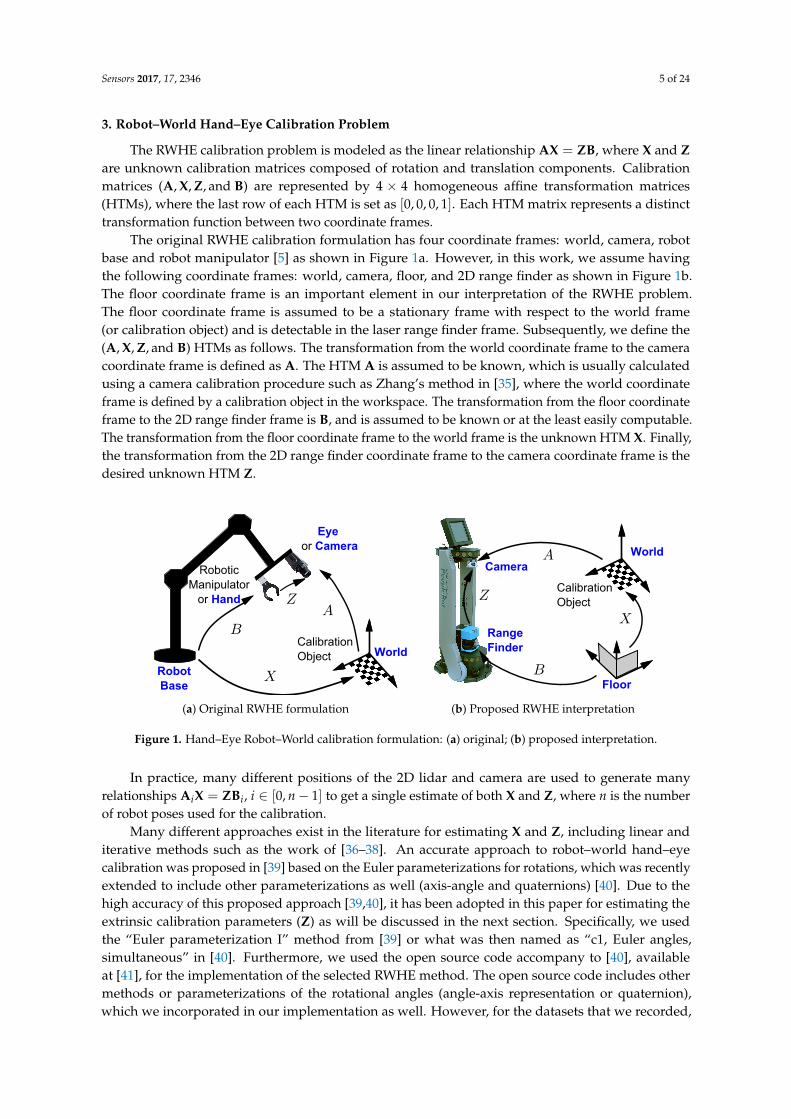
The RWHE calibration problem is modeled as the linear relationship AX = ZB, where X and Zare unknown calibration matrices composed of rotation and translation components. Calibrationmatrices (A, X, Z, and B) are represented by 4 × 4 homogeneous affine transformation matrices(HTMs), where the last row of each HTM is set as [0, 0, 0, 1]. Each HTM matrix represents a distincttransformation function between two coordinate frames.

The original RWHE calibration formulation has four coordinate frames: world, camera, robotbase and robot manipulator [5] as shown in Figure 1a. However, in this work, we assume havingthe following coordinate frames: world, camera, floor, and 2D range finder as shown in Figure 1b.The floor coordinate frame is an important element in our interpretation of the RWHE problem.The floor coordinate frame is assumed to be a stationary frame with respect to the world frame(or calibration object) and is detectable in the laser range finder frame. Subsequently, we define the(A, X, Z, and B) HTMs as follows. The transformation from the world coordinate frame to the cameracoordinate frame is defined as A. The HTM A is assumed to be known, which is usually calculatedusing a camera calibration procedure such as Zhang’s method in [35], where the world coordinateframe is defined by a calibration object in the workspace. The transformation from the floor coordinateframe to the 2D range finder frame is B, and is assumed to be known or at the least easily computable.The transformation from the floor coordinate frame to the world frame is the unknown HTM X. Finally,the transformation from the 2D range finder coordinate frame to the camera coordinate frame is thedesired unknown HTM Z.

CalibrationObject

Eye or Camera

World

Robotic Manipulator

or Hand

RobotBase

(a) Original RWHE formulation

World

Floor

CalibrationObject

RangeFinder

Camera

(b) Proposed RWHE interpretation

Figure 1. Hand–Eye Robot–World calibration formulation: (a) original; (b) proposed interpretation.

In practice, many different positions of the 2D lidar and camera are used to generate manyrelationships AiX = ZBi, i ∈ [0, n− 1] to get a single estimate of both X and Z, where n is the numberof robot poses used for the calibration.

Many different approaches exist in the literature for estimating X and Z, including linear anditerative methods such as the work of [36–38]. An accurate approach to robot–world hand–eyecalibration was proposed in [39] based on the Euler parameterizations for rotations, which was recentlyextended to include other parameterizations as well (axis-angle and quaternions) [40]. Due to thehigh accuracy of this proposed approach [39,40], it has been adopted in this paper for estimating theextrinsic calibration parameters (Z) as will be discussed in the next section. Specifically, we usedthe “Euler parameterization I” method from [39] or what was then named as “c1, Euler angles,simultaneous” in [40]. Furthermore, we used the open source code accompany to [40], availableat [41], for the implementation of the selected RWHE method. The open source code includes othermethods or parameterizations of the rotational angles (angle-axis representation or quaternion),which we incorporated in our implementation as well. However, for the datasets that we recorded,

Sensors 2017, 17, 2346 6 of 24

Euler parameterization I comparably gave the best estimated results without singularity issues, hence itwas selected in this paper. In the event of singularity issues, other parameterizations can be consideredwith little impact on our proposed approach.

4. The Proposed Calibration Procedure

The proposed RWHE calibration formulation consists of the following steps:

1. Select a configuration that relates the lidar–camera sensors together.2. Define the calibration environment with respect to the RWHE coordinate frames (world, camera,

floor, and 2D range finder) and the transformation matrices (A, B, X, Z).3. Compute the transformation matrices A and B.4. Apply the selected RWHE Euler parameterization I method to estimate the desired extrinsic

calibration parameters Z.5. Verify the accuracy of the estimated extrinsic calibration results.

In what follows, the above steps are discussed in detail.

4.1. Camera–Lidar Configurations

To compute the calibration parameters, we considered the following camera–lidar configurations:

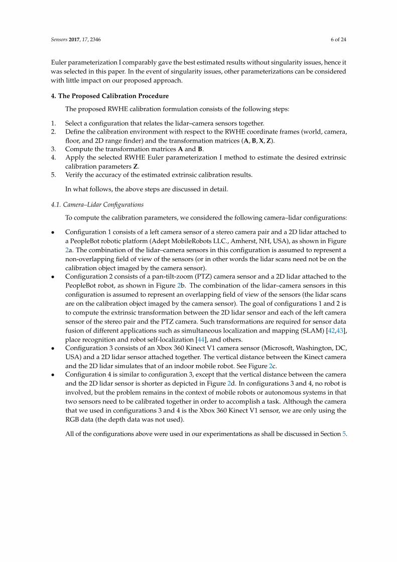
• Configuration 1 consists of a left camera sensor of a stereo camera pair and a 2D lidar attached toa PeopleBot robotic platform (Adept MobileRobots LLC., Amherst, NH, USA), as shown in Figure2a. The combination of the lidar–camera sensors in this configuration is assumed to represent anon-overlapping field of view of the sensors (or in other words the lidar scans need not be on thecalibration object imaged by the camera sensor).

• Configuration 2 consists of a pan-tilt-zoom (PTZ) camera sensor and a 2D lidar attached to thePeopleBot robot, as shown in Figure 2b. The combination of the lidar–camera sensors in thisconfiguration is assumed to represent an overlapping field of view of the sensors (the lidar scansare on the calibration object imaged by the camera sensor). The goal of configurations 1 and 2 isto compute the extrinsic transformation between the 2D lidar sensor and each of the left camerasensor of the stereo pair and the PTZ camera. Such transformations are required for sensor datafusion of different applications such as simultaneous localization and mapping (SLAM) [42,43],place recognition and robot self-localization [44], and others.

• Configuration 3 consists of an Xbox 360 Kinect V1 camera sensor (Microsoft, Washington, DC,USA) and a 2D lidar sensor attached together. The vertical distance between the Kinect cameraand the 2D lidar simulates that of an indoor mobile robot. See Figure 2c.

• Configuration 4 is similar to configuration 3, except that the vertical distance between the cameraand the 2D lidar sensor is shorter as depicted in Figure 2d. In configurations 3 and 4, no robot isinvolved, but the problem remains in the context of mobile robots or autonomous systems in thattwo sensors need to be calibrated together in order to accomplish a task. Although the camerathat we used in configurations 3 and 4 is the Xbox 360 Kinect V1 sensor, we are only using theRGB data (the depth data was not used).

All of the configurations above were used in our experimentations as shall be discussed in Section 5.

Sensors 2017, 17, 2346 7 of 24

Z

Y

X

ExtrinsicTransformationto be computed

Z

YX

Range Finder SensorCoordinate Frame

The Coordinate Frame of the Left Camera of the Stereo Pair

Stereo Camera Pair

RangeFinder Sensor

Left Camera Sensor

(a) Configuration 1

Z

YX

Range Finder SensorCoordinate Frame

X Z

-Y

PTZ Camera Coordinate Frame

ExtrinsicTransformationto be computed

RangeFinder Sensor

PTZ Camera

(b) Configuration 2

(c) Configuration 3 (d) Configuration 4

Figure 2. Four configurations of lidar–camera sensors: (a) SICK LMS-500 2D lidar (Minneapolis, MN,USA) and a mobileRanger C3D stereo camera (Focus Robotics, Hudson, NH, USA) rigidly attachedto a PeopleBot robotic platform; (b) SICK LMS-500 2D lidar and AXIS 214 PTZ network camera(Axis Communications, Lund, Sweden) rigidly attached to a PeopleBot robotic platform; (c) SICKLMS-100 2D lidar and a Kinect Xbox 360 camera rigidly attached at a height similar to a mobile robot;(d) same configuration as of (c), but the camera is mounted at a shorter vertical distance from the lidar.

4.2. Calibration Environment

To apply the RWHE formulation AX = ZB on the underlying extrinsic calibration problem,we need to further discuss the involved coordinate frames introduced in Section 3.

From the standard RWHE calibration problem, there is the world coordinate frame that is definedby a stationary calibration object. In this work, we decided to use a planar chessboard pattern. There isalso the floor coordinate frame that serves as the reference coordinate frame for the lidar sensor.As mentioned before, the main requirement on this floor frame is to be a stationary with respect to thecalibration object and detectable by the lidar sensor. A corner of a wall in the calibration workspacewas chosen for this floor frame, using the assumption that the wall planes are orthogonal. This is

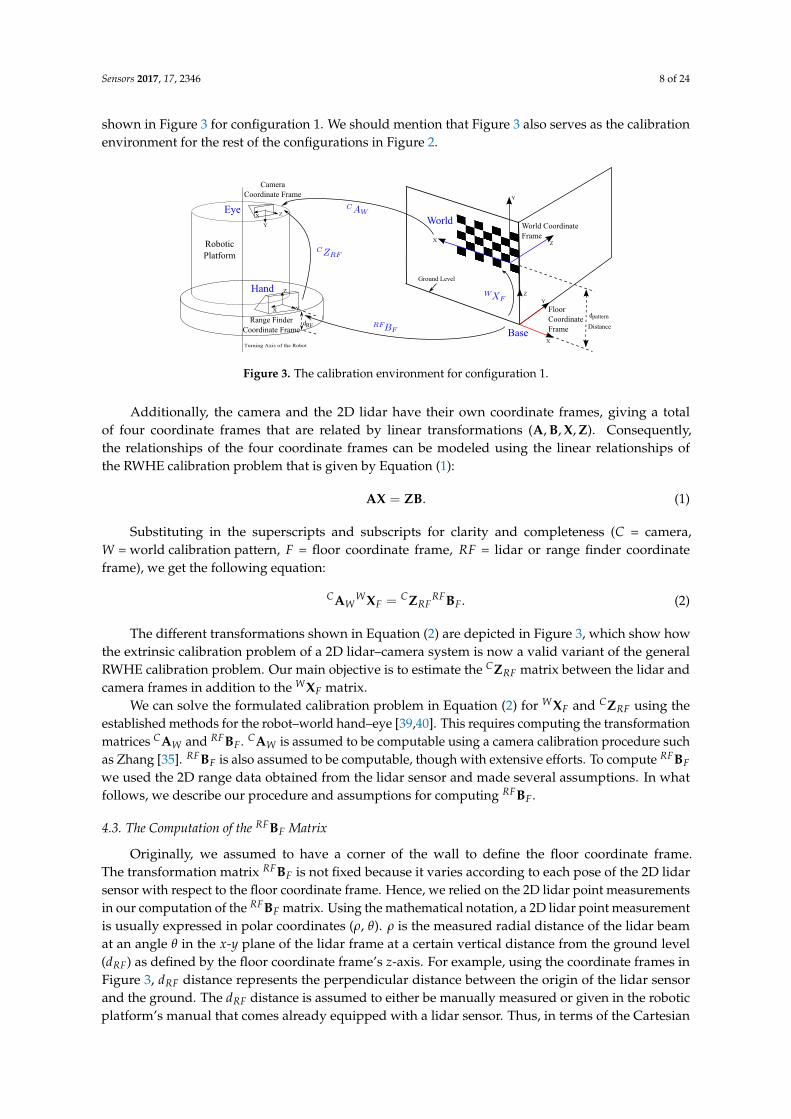
Sensors 2017, 17, 2346 8 of 24

shown in Figure 3 for configuration 1. We should mention that Figure 3 also serves as the calibrationenvironment for the rest of the configurations in Figure 2.

Hand Z

YX

Z

Y

X

Turning Axis of the Robot

XZ

Y

EyeWorld

Base

Z

Robotic

Platform

dpattern

Ground Level

World Coordinate

Frame

X

Y

Floor

Coordinate

Frame Distance

Camera

Coordinate Frame

Range Finder

Coordinate FramedRF

Figure 3. The calibration environment for configuration 1.

Additionally, the camera and the 2D lidar have their own coordinate frames, giving a totalof four coordinate frames that are related by linear transformations (A, B, X, Z). Consequently,the relationships of the four coordinate frames can be modeled using the linear relationships ofthe RWHE calibration problem that is given by Equation (1):

AX = ZB. (1)

Substituting in the superscripts and subscripts for clarity and completeness (C = camera,W = world calibration pattern, F = floor coordinate frame, RF = lidar or range finder coordinateframe), we get the following equation:

CAWWXF = CZRF

RFBF. (2)

The different transformations shown in Equation (2) are depicted in Figure 3, which show howthe extrinsic calibration problem of a 2D lidar–camera system is now a valid variant of the generalRWHE calibration problem. Our main objective is to estimate the CZRF matrix between the lidar andcamera frames in addition to the WXF matrix.

We can solve the formulated calibration problem in Equation (2) for WXF and CZRF using theestablished methods for the robot–world hand–eye [39,40]. This requires computing the transformationmatrices CAW and RFBF. CAW is assumed to be computable using a camera calibration procedure suchas Zhang [35]. RFBF is also assumed to be computable, though with extensive efforts. To compute RFBFwe used the 2D range data obtained from the lidar sensor and made several assumptions. In whatfollows, we describe our procedure and assumptions for computing RFBF.

4.3. The Computation of the RFBF Matrix

Originally, we assumed to have a corner of the wall to define the floor coordinate frame.The transformation matrix RFBF is not fixed because it varies according to each pose of the 2D lidarsensor with respect to the floor coordinate frame. Hence, we relied on the 2D lidar point measurementsin our computation of the RFBF matrix. Using the mathematical notation, a 2D lidar point measurementis usually expressed in polar coordinates (ρ, θ). ρ is the measured radial distance of the lidar beamat an angle θ in the x-y plane of the lidar frame at a certain vertical distance from the ground level(dRF) as defined by the floor coordinate frame’s z-axis. For example, using the coordinate frames inFigure 3, dRF distance represents the perpendicular distance between the origin of the lidar sensorand the ground. The dRF distance is assumed to either be manually measured or given in the roboticplatform’s manual that comes already equipped with a lidar sensor. Thus, in terms of the Cartesian

Sensors 2017, 17, 2346 9 of 24

coordinates, a lidar point measurement (x, y, z) at certain angular resolution can be expressed in thelidar frame as described below:

x = ρ× cos(θ),y = ρ× sin(θ),

z = 0.(3)

During the calibration procedure, we assume that the calibration data is being recorded duringstop and go mode of the robotic platform against the calibration object as shown in Figure 3.The calibration data contains an image of the calibration object and a lidar scan at each positionof the robot platform (or lidar–camera pair) as recorded by the camera and lidar sensors. Each recordedlidar scan consists of a large number of lidar point measurements. The lidar points from each lidarscan are supplied to a linear least squares line fitting procedure to generate a 2D line map. This mapis used to compute the RFBF matrix after locating the origin of the floor frame with respect to theorigin of the lidar frame (i.e., (0,0) location on the map). Locating the origin of the floor frame withinthe map allows computation of three translational components (xt, yt and dRF) and one rotationalcomponent (φ) between the origins of the floor and lidar frames of the RFBF matrix. This provides thetransformation RFBF under the assumption that the lidar scans are all parallel to the floor x-y plane(i.e., the roll and pitch angles of the lidar are zeros). We understand that this assumption might beconsidered a limitation of the proposed work; however, this will mainly affect how the rotationalcomponents of the RFBF matrix are computed. We believe that the presented work with such anassumption can be tolerated as to just prove the main idea of applying the RWHE formulation for theextrinsic lidar–camera calibration with no overlapping field of views of the sensors. The computedRFBF matrix is expressed as given in Equation (4). Figure 4 summarizes the steps taken to compute theRFBF matrix for one pose of the lidar–camera pair:

RFBF =

cos(φ) −sin(φ) 0 xt

sin(φ) cos(φ) 0 yt

0 0 1 −dRF0 0 0 1

. (4)

ym

m

CalibrationTarget

Corner on the Floor

2D Lidar

−3 −2 −1 0 10

1

2

Floor

x mm

ym

m

−2 −1 0 1

0.511.522.5

Real Scene Diagram depicting real scene

(xt , yt)

phi

x mm

x103

x103

x103

x103

robot

Diagram depicting lidar point measurements

Diagram depicting fitted lines of lidar point measurements

Figure 4. Steps to estimate the RFBF matrix.

Sensors 2017, 17, 2346 10 of 24

4.4. Solving the Extrinsic Calibration Parameters

After computing the transformations CAW and RFBF, the WXF and CZRF transformations canbe estimated using the Euler parameterization I method [39]. In Euler parameterization I, the costfunction to be minimized is given in Equation (5), where CAW,i represents the ith camera pose.The transformations WXF and CZRF are decomposed into rotation and translation components asshown in Equation (6). Therefore, in the minimization process, we have a function of 12 variables:three Euler angles and three translation components for each of the WXF and CZRF matrices:

c1 =n−1

∑i=0||CAW,i

WXF − CZRFRFBF,i||2, (5)

c1 =n−1

∑i=0

∥∥∥∥∥∥∥∥∥Ai

RX(θa, θb, θc)

tX0

tX1

tX2~0 1

− RZ(θd, θe, θ f )

tZ0

tZ1

tZ2~0 1

Bi

∥∥∥∥∥∥∥∥∥2

. (6)

The overall minimization problem is shown in Equation (7):

{θa, θb, θc, tX0, tX1, tX2, θd, θe, θ f , tZ0, tZ1, tZ2} = arg minθa ,θb ,θc ,tX0,tX1,tX2θd ,θe ,θ f ,tZ0,tZ1,tZ2

c1. (7)

An approximate solution to Equation (7) is found using an L2 norm with theLevenberg–Marquardt method for nonlinear least squares, as provided by the implementationlevmar [45]. (The initial solutions of θa, θb, θc, θd, θe, θ f are set to zeros such that the correspondingrotational matrices are identity, and similarly the translation components are set to zero. It is importantto mention that for the selected RWHE method, as quoted from [40], “various different initial solutionswere tested, and there was small or negligible difference in the solution quality versus using an identitymatrix for rotation matrices and translation component with all elements zero. For this reason, weconclude that for the experiments ... for the first class of methods is not sensitive to initial solutions”.Therefore, the reader should notice that, with initial solutions as set above, the proposed extrinsiccalibration approach will still converge even if the orientations of the camera and the lidar are highlynot aligned (i.e., a rotation that is not being closed to the identity) as well as a translation that isnot fairly easy to estimate.) Then, substituting in the estimated parameters gives WXF and CZRF inapproximate forms W XF and CZRF as shown in Equations (8) and (9):

W XF =

RX(θa, θb, θc)

tX0

tX1

tX2~0 1

, (8)

CZRF =

RZ(θd, θe, θ f )

tZ0

tZ1

tZ2~0 1

. (9)

The transformations W XF and CZRF will have an ambiguity in the translation components. This isexplained as follows. The reader should note that since the used lidar is only a 2D sensor, the distancebetween the world coordinate frame and the floor coordinate frame is not constrained by Equation (5).Moreover, in the calibration procedure, when we recorded our calibration datasets, the calibrationobject was assumed to be stationary with a moving robotic platform against it. Hence, consideringthe sensors attached to a heavy weight robot platform, similar to the ∼25 Kg PeopleBot platform inour configurations 1 and 2, we will have a problem in our recorded datasets. The problem is that the

Sensors 2017, 17, 2346 11 of 24

moving robot platform will not have tilting poses during the calibration procedure. This results in thatthe recorded calibration datasets lack any excitation in the roll and pitch angles, which in turn rendersthe mounting height of the camera unobservable and accordingly an ambiguity in the translationalcomponents of the estimated extrinsic parameters. However, we can create a constraint and solve thisproblem by manually measuring a defined distance that we call dpattern. dpattern distance is defined asthe distance (in terms of the world coordinate frame’s y axis) from the (0, 0, 0) location of the calibrationobject to the ground plane. However, other configurations of the world frame are possible, such as inFigure 5. In this case, to find dpattern distance, some trigonometry is needed in terms of measuring theperpendicular distance from the origin of the world frame along the y-axis to the ground.

Zdpattern

Ground Level

WorldCoordinateFrame Y

FloorCoordinateFrame

Distance

X

X

Y

Figure 5. Schematic view of possible orientation of the world coordinate system.

When the value of dpattern is known, we can specify that the y translation component of WXF is−dpattern as shown in Equation (10):

W XF =

RX(θa, θb, θc)

tX0

−dpattern

tX2~0 1

. (10)

While it is possible to adjust W XF with a constant such that the translational ambiguity is resolved,in order to reconcile CZRF to that change, another Levenberg–Marquardt minimization procedure isrecommended to be performed.

Consequently, we minimize the function c1 in Equation (6) via another application of theLevenberg–Marquardt method, but this time with one less parameter. This is because the y componentof the translation in W XF will remain constant as −dpattern. The minimization problem is shownin Equation (11); the initial solution given to the Levenberg–Marquardt method is W XF and CZRF.The new approximate solutions W ˆXF and C ˆZRF are produced by substituting the estimated parametersas in Equations (8) and (9) and ˆtX1 = −dpattern:

{ ˆθa, ˆθb, ˆθc, ˆtX0, ˆtX2ˆθd, ˆθe, ˆθ f , ˆtZ0, ˆtZ1, ˆtZ2} = arg min

θa ,θb ,θc ,tX0,tX2θd ,θe ,θ f ,tZ0,tZ1,tZ2

c1. (11)

Algorithm 1 summarizes the process of estimating the transformations W ˆXF and C ˆZRF. It isrecommended that the order in Algorithm 1 of lines 3, 5, and 6 is maintained. The reason is that thesearch for an approximate local minimum gets stuck in poorer quality estimates of WXF and CZRF ifthis order is not followed. Of course, this behavior is method and dataset dependent. In addition, it

Sensors 2017, 17, 2346 12 of 24

may not be true in all situations, but, through experimentation, it was found true with the datasetsthat we used in this work.

Algorithm 1 Perform calibration of two sensors

1: Compute CAW,i for each pose i.2: Compute RFBF,i for each pose i.3: Compute solution to Equation (7) using 12 parameters, using zeros as initial solutions for all

parameters. This solution is W XF and CZRF.4: Manually measure the dpattern distance.5: Set the y translational component of W XF to −dpattern as in Equation (10).

6: Compute W ˆXF and C ˆZRF, which are the approximate solution to Equation (11) using 11 parameters,where W XF and CZRF (from line 3) serve as the initial solution.

4.5. Verifying Accuracy

With the extrinsic calibration results C ˆZRF and W ˆXF estimated using Algorithm 1, the laser datafrom the 2D lidar can be projected onto the imaging plane of the camera sensor. This will be animportant step to check the accuracy of the estimated results. To this end, we next discuss how a givenlidar point measurement is projected onto the camera sensor plane.

To project a homogeneous point ~Xi defined with respect to the lidar coordinate frame(see Equation (3)) onto a point~xi in the image plane of a camera sensor, we can use the followingforward projection relationship:

~xi = K ˆZ3×4 ~Xi, (12)

where~xi is composed of a (3× 1) homogeneous vector, ~Xi is composed of a (4× 1) homogeneousvector (the third z component is zero), K3×3 is the intrinsic camera calibration matrix, and ˆZ3×4 isC ˆZRF without the last row (i.e., [0, 0, 0, 1]). The relationship in Equation (12) assumes either zero radialand tangential distortion or that such distortion has already been removed.

Similarly, with the estimated calibration results (C ˆZRF and W ˆXF), the world calibration points onthe calibration pattern can be projected onto the imaging plane using a newly estimated A matrix thatwe refer to as Anew = C ˆZRF

RFBFW ˆX−1

F matrix. This is done using the forward projection equationas follows:

~xi = KAnew3×4~Xi, (13)

where~xi is again composed of a (3× 1) homogeneous vector, ~Xi is composed of a (4× 1) homogeneousvector in the world coordinate frame, K3×3 is the intrinsic camera calibration matrix, and Anew3×4

is Anew without the last row. The relationship in Equation (13) also assumes either zero radial andtangential distortion or that such distortion has already been removed.

Subsequently, we could check the accuracy of the estimated calibration results C ˆZRF and W ˆXF,by computing the reprojection root mean squared error (rrmse). The rrmse is computed betweenprojected world calibration points (i.e., the grid points of the calibration object) to the image planeusing the original A matrix and the same world calibration points projected using the Anew matrix.This rrmse computation is given in Equation (14):

rrmse =

√1m

m

∑i‖~xi,new −~xi‖2, (14)

where i is an image point index, m total number of world projected calibration points,~xi,new = KAnew3×4

~Xi, and~xi = KA3×4 ~Xi.

Sensors 2017, 17, 2346 13 of 24

5. Experimental Results

This section presents the experimental extrinsic calibration results for the four configurationsshown in Figure 2. For configurations 1 and 2, in Figure 2a,b, a SICK-LMS 500 lidar is used. This lidarwas set to an angular resolution of 0.5◦ and 180◦ angular field of view. For configurations 3 and 4, inFigure 2c,d, a SICK-LMS 100 is used with an angular resolution of 0.5◦ and 270◦ angular field of view.

In all configurations (1–4), we assume valid and known intrinsic calibration parameters of thecameras. We also assume a pin-hole camera model for the cameras with radial and tangential lensdistortion as described in [35].(It is assumed that, for configurations 1 and 2 in Figure 2, the individualintrinsic camera calibration and the remaining extrinsic transformation, say between the left and rightcamera or between the left camera and the PTZ camera sensors, to be computed using the standardstereo camera calibration [30,46] when needed.) All of the results shown in this paper were generatedon a workstation with two quad-core processors and 8 GB of RAM. The camera calibration was carriedout using the open source computer vision library (i.e., OpenCV’s camera calibration functions) [46],where the calibration object does not have to be moved. The calibration object used in all configurationswas a 9× 7 checkerboard, where the size of a checker square was 40 mm × 40 mm.

The number of calibration images and lidar scans used in configurations 1 and 2 was 18, while 15and 12 were used for configurations 3 and 4, respectively. The number of poses reported above for allof the configurations has no link to the accuracy of the reported results, but rather an indication of theactual poses that was recorded and used to generate the estimated calibration results.

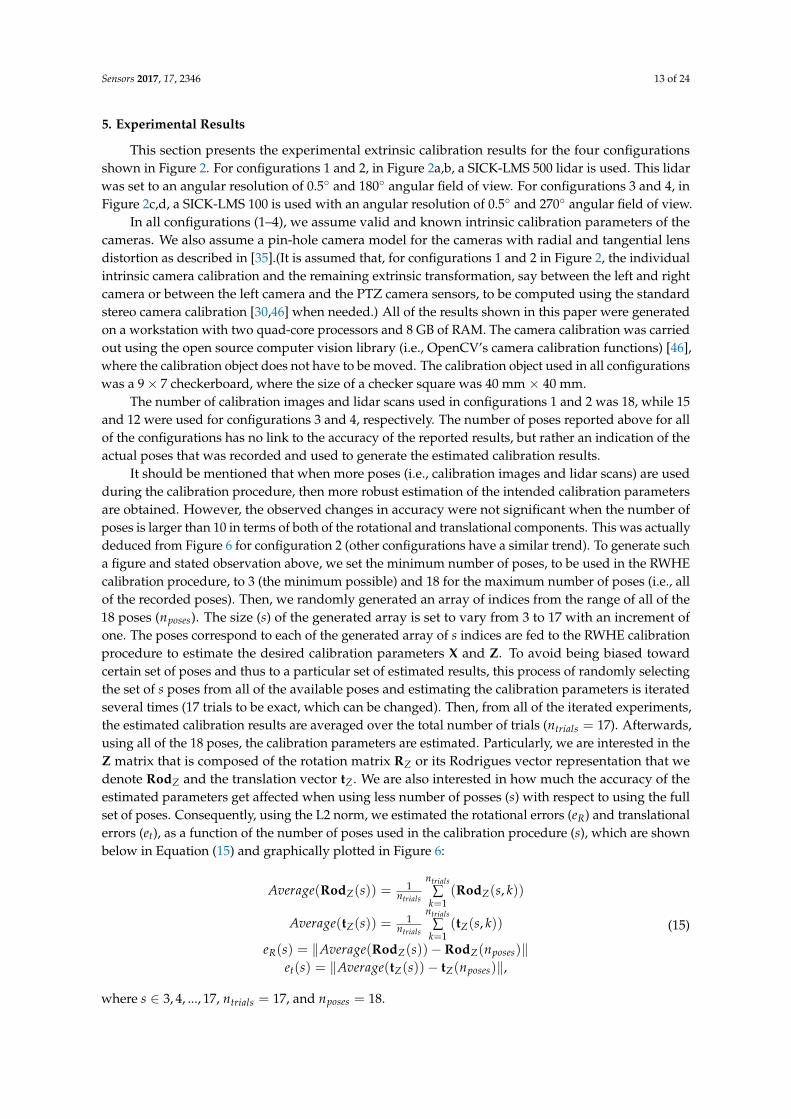
It should be mentioned that when more poses (i.e., calibration images and lidar scans) are usedduring the calibration procedure, then more robust estimation of the intended calibration parametersare obtained. However, the observed changes in accuracy were not significant when the number ofposes is larger than 10 in terms of both of the rotational and translational components. This was actuallydeduced from Figure 6 for configuration 2 (other configurations have a similar trend). To generate sucha figure and stated observation above, we set the minimum number of poses, to be used in the RWHEcalibration procedure, to 3 (the minimum possible) and 18 for the maximum number of poses (i.e., allof the recorded poses). Then, we randomly generated an array of indices from the range of all of the18 poses (nposes). The size (s) of the generated array is set to vary from 3 to 17 with an increment ofone. The poses correspond to each of the generated array of s indices are fed to the RWHE calibrationprocedure to estimate the desired calibration parameters X and Z. To avoid being biased towardcertain set of poses and thus to a particular set of estimated results, this process of randomly selectingthe set of s poses from all of the available poses and estimating the calibration parameters is iteratedseveral times (17 trials to be exact, which can be changed). Then, from all of the iterated experiments,the estimated calibration results are averaged over the total number of trials (ntrials = 17). Afterwards,using all of the 18 poses, the calibration parameters are estimated. Particularly, we are interested in theZ matrix that is composed of the rotation matrix RZ or its Rodrigues vector representation that wedenote RodZ and the translation vector tZ. We are also interested in how much the accuracy of theestimated parameters get affected when using less number of posses (s) with respect to using the fullset of poses. Consequently, using the L2 norm, we estimated the rotational errors (eR) and translationalerrors (et), as a function of the number of poses used in the calibration procedure (s), which are shownbelow in Equation (15) and graphically plotted in Figure 6:

Average(RodZ(s)) = 1ntrials

ntrials∑

k=1(RodZ(s, k))

Average(tZ(s)) = 1ntrials

ntrials∑

k=1(tZ(s, k))

eR(s) = ‖Average(RodZ(s))− RodZ(nposes)‖et(s) = ‖Average(tZ(s))− tZ(nposes)‖,

(15)

where s ∈ 3, 4, ..., 17, ntrials = 17, and nposes = 18.

Sensors 2017, 17, 2346 14 of 24

4 6 8 10 12 14 16 180

0.002

0.004

0.006

0.008

0.01

0.012

3Number of Poses (s) Used in the RWHE Calibartaion Procedure

e R(s)(nounit)

(a)

4 6 8 10 12 14 16 180

2

4

6

8

10

Number of Poses (s) Used in the RWHE Calibartaion Procedure

e t(s)mm

3

(b)

Figure 6. The accuracy of the extrinsic camera calibration parameters as a function of the number ofposes used in the RWHE calibration procedure for configuration 2: (a) rotation error of the estimated Zmatrix; (b) translation error of the estimated Z matrix.

From Figure 6 and related experiments discussed above, we can draw several observations.

• Using few poses produced calibration results comparable to that of large number of poses.• Comparing three poses with 18 poses, the averaged translational errors were just 8 mm and the

averaged rotation errors were just 0.0105 indicating that the presented RWHE calibration methodworks fine with the three poses case (i.e., minimum number of possible poses).

• The most important poses that would mostly affect the accuracy of the results are those posesthat are very close to the calibration pattern, although this was not shown in Figure 6, as weare taking the average of the randomly selected poses over many trials. This observation wasactually discussed in [29], and as such no experimental results about this study were presentedand analyzed further in this paper.

Table 1 lists the manually measured distances dRF and dpattern for the Configurations 1–4.

Table 1. The calibration distances dRF and dpattern for the four configurations in Figure 2.

Measured Distance (mm) Configuration 1 Configuration 2 Configuration 3 Configuration 4

dpattern 830 830 830 160dRF 340 340 140 140

Throughout all of the experiments, once the A and B matrices are determined, the time to estimatethe ˆX and ˆZ transformations is usually less than a minute. Practically speaking, the exact time willdepend on the size of the calibration data supplied to the calibration procedure. Further insight on thetiming performance of the employed RWHE calibration procedure is provided in [40].

Sensors 2017, 17, 2346 15 of 24

For the configurations in Figure 2, configuration 2 allows for overlapping filed of views of thesensors as done in Zhang and Pless method [6]. Hence, it was easier to compare this configurationwith the work in [6].

The rest of the section is organized as follows. First, the calibration results (i.e., the estimated Xand Z transformations) are presented for configurations 1 and 3, when the calibration pattern is not inthe field of view of both the lidar and camera sensors (Section 5.1). Then, the results are discussed forconfigurations 2 and 4, when the lidar and camera sensors view the calibration pattern (Section 5.2).The comparison with the Zhang and Pless method [6] is presented in Section 5.3. The uniqueness ofthe proposed calibration approach is highlighted in Section 5.4.

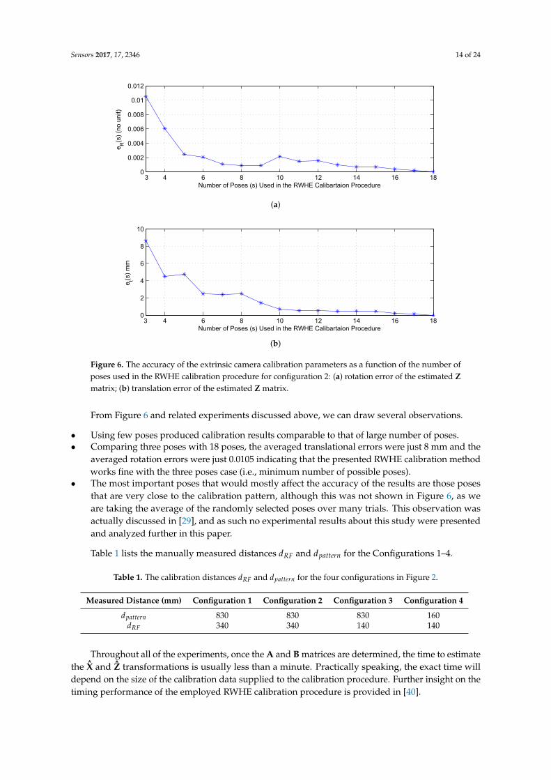
5.1. Calibration Results for Configurations 1 and 3

To estimate the calibration parameters for configurations 1 and 3, we used the correspondingmeasured dpattern and dRF values provided in Table 1. The accuracy of the obtained results is calculatedusing Equation (14).

Figures 7 and 8 show projection of world calibration points (grid points) to one selected calibrationimage in configurations 1 and 3. The error difference between the location of the point in images(based on the original A matrix) and the reprojected point (based on the Anew = ZBX−1 matrix) isshown by a blue line. The rrmse error values are (in pixels); 3.77658 and 5.17108 for configurations1 and 3, respectively. The error values imply high accuracy in the estimated calibration results.

Zoomed

Figure 7. Configuration 1: Reprojection error based on the estimated X and Z matrices. Blue linesindicate the amount of the reprojection error (original image resolution 752× 480).

Zoomed

Figure 8. Configuration 3: Reprojection error based on the estimated X and Z matrices. Blue linesindicate the amount of the reprojection error (original image resolution 640× 480).

Sensors 2017, 17, 2346 16 of 24

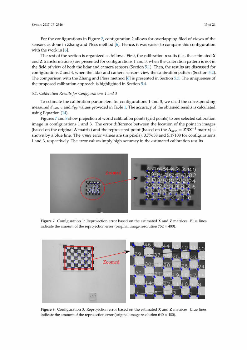
Figures 9 and 10 show forward projection of lidar point measurements to two selected test imagesfor configurations 1 and 3, using the corresponding estimated Z matrix. It should be noted that noground truth of the estimated calibration parameters is available. With visual inspection, the lidarpoints are correctly projected to the image plane, in configurations 1 and 3, at about the same heightof the corresponding lidar from the ground level based on the dRF distance. The verification wasmanually done by measuring the distances of where the lidar points projected on the wall plane(s) oron the calibration object (see next subsection), and then comparing that to the reported dRF values inTable 1. The measured distances of the projected lidar scans to the ground plane were all very closeto the dRF values in Table 1 within 1–5% of an error. While this error is small, it is believed that theerror sources might be due to uncertainties in the estimated intrinsic camera parameters, measureddistances, lidar point measurements, and the computed A and B matrices. This is consistent withthe assumption that the lidar scans are parallel to the ground plane, and shows high accuracy in theestimated calibration results. Similar verification was done for the rest of the configurations.

(a) (b)

Figure 9. Configuration 1: Projection of lidar data to two test images using the estimated Z matrix(points are shown in red color): (a) first test image; (b) second test image.

(a) (b)

Figure 10. Configuration 3: Projection of the lidar data to two test images using the estimated Z matrix(points are shown in red color): (a) first test image; (b) second test image.

Sensors 2017, 17, 2346 17 of 24

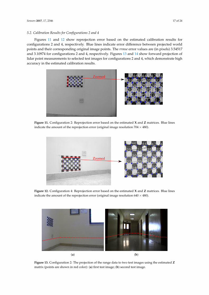
5.2. Calibration Results for Configurations 2 and 4

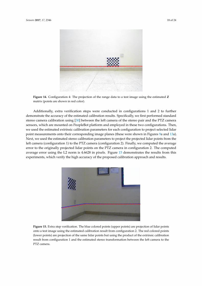
Figures 11 and 12 show reprojection error based on the estimated calibration results forconfigurations 2 and 4, respectively. Blue lines indicate error difference between projected worldpoints and their corresponding original image points. The rrmse error values are (in pixels) 3.54517and 3.10974 for configurations 2 and 4, respectively. Figures 13 and 14 show forward projection oflidar point measurements to selected test images for configurations 2 and 4, which demonstrate highaccuracy in the estimated calibration results.

Zoomed

Figure 11. Configuration 2: Reprojection error based on the estimated X and Z matrices. Blue linesindicate the amount of the reprojection error (original image resolution 704× 480).

Zoomed

Figure 12. Configuration 4: Reprojection error based on the estimated X and Z matrices. Blue linesindicate the amount of the reprojection error (original image resolution 640× 480).

(a) (b)

Figure 13. Configuration 2: The projection of the range data to two test images using the estimated Zmatrix (points are shown in red color): (a) first test image; (b) second test image.

Sensors 2017, 17, 2346 18 of 24

Figure 14. Configuration 4: The projection of the range data to a test image using the estimated Zmatrix (points are shown in red color).

Additionally, extra verification steps were conducted in configurations 1 and 2 to furtherdemonstrate the accuracy of the estimated calibration results. Specifically, we first performed standardstereo camera calibration using [30] between the left camera of the stereo pair and the PTZ camerasensors, which are mounted on PeopleBot platform and employed in these two configurations. Then,we used the estimated extrinsic calibration parameters for each configuration to project selected lidarpoint measurements onto their corresponding image planes (these were shown in Figures 9a and 13a).Next, we used the estimated stereo calibration parameters to project the projected lidar points from theleft camera (configuration 1) to the PTZ camera (configuration 2). Finally, we computed the averageerror to the originally projected lidar points on the PTZ camera in configuration 2. The computedaverage error using the L2 norm is 4.6628 in pixels. Figure 15 demonstrates the results from thisexperiments, which verify the high accuracy of the proposed calibration approach and results.

Figure 15. Extra step verification. The blue colored points (upper points) are projection of lidar pointsonto a test image using the estimated calibration result from configuration 2. The red colored points(lower points) are projection of the same lidar points but using the product of the extrinsic calibrationresult from configuration 1 and the estimated stereo transformation between the left camera to thePTZ camera.

Sensors 2017, 17, 2346 19 of 24

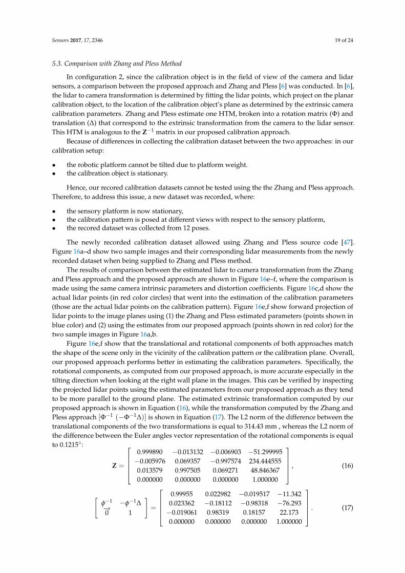
5.3. Comparison with Zhang and Pless Method

In configuration 2, since the calibration object is in the field of view of the camera and lidarsensors, a comparison between the proposed approach and Zhang and Pless [6] was conducted. In [6],the lidar to camera transformation is determined by fitting the lidar points, which project on the planarcalibration object, to the location of the calibration object’s plane as determined by the extrinsic cameracalibration parameters. Zhang and Pless estimate one HTM, broken into a rotation matrix (Φ) andtranslation (∆) that correspond to the extrinsic transformation from the camera to the lidar sensor.This HTM is analogous to the Z−1 matrix in our proposed calibration approach.

Because of differences in collecting the calibration dataset between the two approaches: in ourcalibration setup:

• the robotic platform cannot be tilted due to platform weight.• the calibration object is stationary.

Hence, our recored calibration datasets cannot be tested using the the Zhang and Pless approach.Therefore, to address this issue, a new dataset was recorded, where:

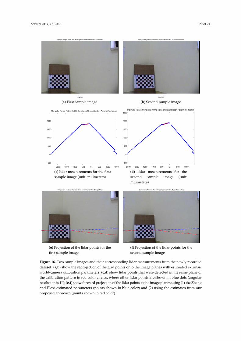
• the sensory platform is now stationary,• the calibration pattern is posed at different views with respect to the sensory platform,• the recored dataset was collected from 12 poses.

The newly recorded calibration dataset allowed using Zhang and Pless source code [47].Figure 16a–d show two sample images and their corresponding lidar measurements from the newlyrecorded dataset when being supplied to Zhang and Pless method.

The results of comparison between the estimated lidar to camera transformation from the Zhangand Pless approach and the proposed approach are shown in Figure 16e–f, where the comparison ismade using the same camera intrinsic parameters and distortion coefficients. Figure 16c,d show theactual lidar points (in red color circles) that went into the estimation of the calibration parameters(those are the actual lidar points on the calibration pattern). Figure 16e,f show forward projection oflidar points to the image planes using (1) the Zhang and Pless estimated parameters (points shown inblue color) and (2) using the estimates from our proposed approach (points shown in red color) for thetwo sample images in Figure 16a,b.

Figure 16e,f show that the translational and rotational components of both approaches matchthe shape of the scene only in the vicinity of the calibration pattern or the calibration plane. Overall,our proposed approach performs better in estimating the calibration parameters. Specifically, therotational components, as computed from our proposed approach, is more accurate especially in thetilting direction when looking at the right wall plane in the images. This can be verified by inspectingthe projected lidar points using the estimated parameters from our proposed approach as they tendto be more parallel to the ground plane. The estimated extrinsic transformation computed by ourproposed approach is shown in Equation (16), while the transformation computed by the Zhang andPless approach [Φ−1 (−Φ−1∆)] is shown in Equation (17). The L2 norm of the difference between thetranslational components of the two transformations is equal to 314.43 mm , whereas the L2 norm ofthe difference between the Euler angles vector representation of the rotational components is equalto 0.1215◦:

Z =

0.999890 −0.013132 −0.006903 −51.299995−0.005976 0.069357 −0.997574 234.4445550.013579 0.997505 0.069271 48.8463670.000000 0.000000 0.000000 1.000000

, (16)

[φ−1 −φ−1∆−→0 1

]=

0.99955 0.022982 −0.019517 −11.342

0.023362 −0.18112 −0.98318 −76.293−0.019061 0.98319 0.18157 22.1730.000000 0.000000 0.000000 1.000000

. (17)

Sensors 2017, 17, 2346 20 of 24

reproject the grid points onto the image with estimated extrinsic parameters

Longitude

(a) First sample image

reproject the grid points onto the image with estimated extrinsic parameters

Longitude

(b) Second sample image

−2000 −1500 −1000 −500 0 500 1000 1500

−500

0

500

1000

1500

2000

Plot Valid Range Points that hit the plane of the calibration Pattern (Red color)

(c) lidar measurements for the firstsample image (unit: milimeters)

−2500 −2000 −1500 −1000 −500 0 500 1000

−500

0

500

1000

1500

2000

2500Plot Valid Range Points that hit the plane of the calibration Pattern (Red color)

(d) lidar measurements for thesecond sample image (unit:milimeters)

Comparative Analysis: Red color Using our estimates, Blue: Zhang &Pless

(e) Projection of the lidar points for thefirst sample image

Comparative Analysis: Red color Using our estimates, Blue: Zhang &Pless

(f) Projection of the lidar points for thesecond sample image

Figure 16. Two sample images and their corresponding lidar measurements from the newly recordeddataset. (a,b) show the reprojection of the grid points onto the image planes with estimated extrinsicworld-camera calibration parameters; (c,d) show lidar points that were detected in the same plane ofthe calibration pattern in red color circles, where other lidar points are shown in blue dots (angularresolution is 1◦); (e,f) show forward projection of the lidar points to the image planes using (1) the Zhangand Pless estimated parameters (points shown in blue color) and (2) using the estimates from ourproposed approach (points shown in red color).

Sensors 2017, 17, 2346 21 of 24

5.4. Uniqueness of the Proposed Approach

The presented approach in this paper share many similarities that come from both Zhang andPless [6] and Bok et al. [29]. In this subsection, the added values of our approach are highlighted.

While our proposed approach and that of Zhang and Pless similarly estimate the desired extrinsiccalibration parameters, our approach does not require that the camera–lidar sensors share a commonfield of view of the calibration object. Both approaches estimate the desired extrinsic calibrationparameters by minimizing the distance between the plane of the calibration pattern and the locationof the pattern as estimated by the camera. However, our approach casts the problem using theRWHE calibration formulation and considers different assumptions about the scene and the calibrationprocedure. Compared with the Zhang and Pless approach, our calibration paradigm is considered aharder problem because the field of views of the sensors need not overlap, and the moving roboticplatform may not be tilted during calibration due to many reasons such as a heavy mobile robotbase. The sensory platform weight leads to the problem in that the recorded calibration datasetlacks any excitation in the roll and pitch angles and thus having some of the extrinsic calibrationparameters be unobservable. This was successfully mitigated by using manually measured dpattern

distance. Additionally, having the robot platform moving against a stationary calibration target allowsfor automatic or semi-automatic robot platform self-calibration (considering the manually measureddistances dpattern and dRF), which is not feasible with the Zhang and Pless approach.

Comparing our approach with Bok et al. [29], both approaches deal with no-overlap extrinsiccalibration of a lidar–camera systems and also adopt some reasonable assumptions about the calibrationenvironment. However, there are few differences between the two approaches. First, Bok et al. definedeither a plane perpendicular to one of the axes of the world coordinate system (as defined by thecalibration pattern), or a line intersecting two planes that is parallel to one of the axes of the worldcoordinate system to perform the calibration. In our approach, we defined a corner on the floor andrequired that the lidar scans are to be parallel to the ground plane. Second, the approach by Boket al. requires manual selection of lidar data that overlapped the defined geometric structure. Inour proposed approach, the manual selection of lidar data is not required; instead, dpattern and dRFdistances are assumed to be manually measured. Lastly, the nonlinear optimization cost function usedin the Bok et al. approach is structure dependent, where in our approach the cost function is structureindependent and only associated with the employed RWHE calibration approach.

Finally, our proposed approach is flexible and scalable to consider other configurations or setups.For example, one could add many other lidars and cameras and be very flexible with the presentedapproach to estimate the calibration parameters. The only requirement is to compute the transformationmatrices (As and Bs) for the RWHE method to estimate the desired calibration parameters X and Z.In addition, one may need to consider fixing the translational components of the estimated matricessimilar to what was done when we fixed the y translational component of the W XF matrix in Equation(10) to remove the translational ambiguity.

6. Conclusions

This paper presented a novel approach for the extrinsic calibration of a camera–lidar systemwithout overlap based on a RWHE calibration problem. The system was mapped to the RWHEcalibration problem and the transformation matrix B was computed, by considering reasonableassumptions about the calibration environment. The calibration results of various experiments andconfigurations were analyzed. The accuracy of the results was examined and verified. Our approachwas compared to a state-of-the-art method in extrinsic 2D lidar to camera calibration. Results indicatethat the proposed approach provides better accuracy with an L2 norm translational and rotationaldeviations of 314 mm and 0.12◦, respectively.

The presented work is unique, flexible, and scalable. Our approach is considered one of the fewstudies addressing the topic of target-based extrinsic calibration with no overlap. We believe that itcan easily be a part of an automatic robotic platform self-calibration assuming the required distances

Sensors 2017, 17, 2346 22 of 24

(i.e., dRF and dpattern) are known. Additionally, we could add other lidars and cameras to the proposedsystem and still be capable of using the proposed calibration approach.

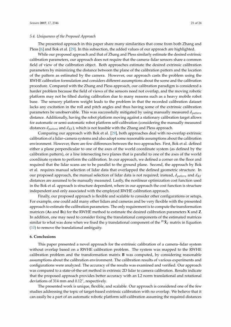
Future work could consider applying the presented ideas to other robotic platforms with possiblydifferent placements of the heterogeneous sensors after deciding the possible importance of suchconfigurations in the robotic and computer vision communities. For example, Figure 17 illustratesa system of a camera and 2D lidar sensors with a non-overlapping field of view, and the views ofthe sensors are in completely different planes. Considering the possible sources of uncertainties inthe calibration procedure, and thus in the estimated parameters, is another point of future work.Furthermore, future work may possibly include researching the calibration problem when the lidarsensor on the robotic platform is being tilted such that the lidar scans are not being parallel to theground floor anymore.

Figure 17. A configuration where the views of the sensors are in different planes.

Acknowledgments: We would like to acknowledge that this research was supported by a grant from theDeanship of Scientific Research at the Hashemite University, Zarqa, Jordan. In addition, we would like to thankAmy Tabb of the United States Department of Agriculture, Agricultural Research Service, the Appalachian FruitResearch Station (USDA-ARS-AFRS) for her valuable discussions on this research topic.

Author Contributions: Khalil Ahmad Yousef was responsible for the algorithm development, data collection,the experimental study, and the writing of the paper. Bassam Mohd provided technical support, guidance throughthe project and contributed to the paper writing and editing. Khalid Al-Widyan contributed to analysis of theexperimental results. Thaier Hayajneh helped in organizing the work and editing the paper.

Conflicts of Interest: The authors declare no conflict of interest.

References

1. Yu, L.; Peng, M.; You, Z.; Guo, Z.; Tan, P.; Zhou, K. Separated Calibration of a Camera and a LaserRangefinder for Robotic Heterogeneous Sensors. Int. J. Adv. Robot. Syst. 2013, 10, 367.

2. Underwood, J.; Hill, A.; Scheding, S. Calibration of range sensor pose on mobile platforms. In Proceedingsof the International Conference on Intelligent Robots and Systems, 2007 (IROS 2007), San Diego, CA, USA,29 October–2 November 2007; pp. 3866–3871.

3. Cucci, D.A.; Matteucci, M. A Flexible Framework for Mobile Robot Pose Estimation and Multi-SensorSelf-Calibration. In Proceedings of the International Conference on Informatics in Control, Automation andRobotics (ICINCO), Reykjavík, Iceland, 29–31 July 2013; pp. 361–368.

4. Ahmad Yousef, K. Hypothesize-and-Verify Based Solutions for Place Recognition and Mobile RobotSelf-Localization in Interior Hallways. Ph.D. Thesis, Purdue University, West Lafayette, IN, USA, 2013.

5. Zhuang, H.; Roth, Z.S.; Sudhakar, R. Simultaneous robot/world and tool/flange calibration by solvinghomogeneous transformation equations of the form AX=YB. IEEE Trans. Robot. Autom. 1994, 10, 549–554.

Sensors 2017, 17, 2346 23 of 24

6. Zhang, Q.; Pless, R. Extrinsic calibration of a camera and laser range finder (improves camera calibration).In Proceedings of the IEEE/RSJ International Conference on Intelligent Robots and Systems, 2004 (IROS 2004),Sendai, Japan, 8 September–2 October 2004; Voume 3, pp. 2301–2306.

7. Vasconcelos, F.; Barreto, J.P.; Nunes, U. A minimal solution for the extrinsic calibration of a camera and alaser-rangefinder. IEEE Trans. Pattern Anal. Mach. Intell. 2012, 34, 2097–2107.

8. Hu, Z.; Li, Y.; Li, N.; Zhao, B. Extrinsic Calibration of 2-D Laser Rangefinder and Camera From Single ShotBased on Minimal Solution. IEEE Trans. Instrum. Meas. 2016, 65, 915–929.

9. Furgale, P.; Rehder, J.; Siegwart, R. Unified temporal and spatial calibration for multi-sensor systems.In Proceedings of the IEEE/RSJ International Conference on Intelligent Robots and Systems (IROS), Tokyo,Japan, 3–7 November 2013; pp. 1280–1286.

10. Gao, C.; Spletzer, J.R. On-line calibration of multiple LIDARs on a mobile vehicle platform. In Proceedingsof the IEEE International Conference on Robotics and Automation (ICRA), Anchorage, AK, USA, 3–7 May2010; pp. 279–284.

11. Svoboda, T.; Martinec, D.; Pajdla, T. A convenient multicamera self-calibration for virtual environments.PRESENCE Teleoper. Virtual Environ. 2005, 14, 407–422.

12. Heng, L.; Li, B.; Pollefeys, M. Camodocal: Automatic intrinsic and extrinsic calibration of a rig with multiplegeneric cameras and odometry. In Proceedings of the IEEE/RSJ International Conference on IntelligentRobots and Systems, Tokyo, Japan, 3–7 November 2013; pp. 1793–1800.

13. Levinson, J.; Thrun, S. Automatic Online Calibration of Cameras and Lasers. In Proceedings of the Robotics:Science and Systems, Berlin, Germany, 24–28 June 2013.

14. Pandey, G.; McBride, J.R.; Savarese, S.; Eustice, R.M. Automatic extrinsic calibration of vision and lidar bymaximizing mutual information. J. Field Robot. 2015, 32, 696–722.

15. Castorena, J.; Kamilov, U.S.; Boufounos, P.T. Autocalibration of LIDAR and optical cameras via edgealignment. In Proceedings of the IEEE International Conference on Acoustics, Speech and Signal Processing(ICASSP), Shanghai, China, 20–25 March 2016; pp. 2862–2866.

16. Napier, A.; Corke, P.; Newman, P. Cross-calibration of push-broom 2d lidars and cameras in naturalscenes. In Proceedings of the IEEE International Conference on Robotics and Automation (ICRA), Karlsruhe,Germany, 6–10 May 2013; pp. 3679–3684.

17. Li, G.; Liu, Y.; Dong, L.; Cai, X.; Zhou, D. An algorithm for extrinsic parameters calibration of a cameraand a laser range finder using line features. In Proceedings of the IEEE/RSJ International Conference onIntelligent Robots and Systems, San Diego, CA, USA, 29 October–2 November 2007; pp. 3854–3859.

18. Gong, X.; Lin, Y.; Liu, J. 3D LIDAR-camera extrinsic calibration using an arbitrary trihedron. Sensors 2013,13, 1902–1918.

19. Sim, S.; Sock, J.; Kwak, K. Indirect correspondence-based robust extrinsic calibration of LiDAR and camera.Sensors 2016, 16, 933.

20. Wasielewski, S.; Strauss, O. Calibration of a multi-sensor system laser rangefinder/camera. In Proceedingsof the Intelligent Vehicles’ 95 Symposium, Detroit, MI, USA, 25–26 September 1995; pp. 472–477.

21. Ha, J.E. Extrinsic calibration of a camera and laser range finder using a new calibration structure of a planewith a triangular hole. Int. J. Control Autom. Syst. 2012, 10, 1240–1244.

22. Shi, K.; Dong, Q.; Wu, F. Weighted similarity-invariant linear algorithm for camera calibration with rotating1-D objects. IEEE Trans. Image Process. 2012, 21, 3806–3812.

23. Mei, C.; Rives, P. Calibration between a central catadioptric camera and a laser range finder for roboticapplications. In Proceedings IEEE International Conference on Robotics and Automation, 2006 (ICRA 2006),Orlando, FL, USA, 15–19 May 2006; pp. 532–537.

24. Krause, S.; Evert, R. Remission based improvement of extrinsic parameter calibration of camera and laserscanner. In Proceedings of the 12th International Conference on Control Automation Robotics & Vision(ICARCV), Guangzhou, China, 5–7 December 2012; pp. 829–834.

25. Li, D.; Tian, J. An accurate calibration method for a camera with telecentric lenses. Opt. Lasers Eng. 2013,51, 538–541.

26. Geiger, A.; Moosmann, F.; Car, O.; Schuster, B. Automatic camera and range sensor calibration using a singleshot. In Proceedigs of the IEEE International Conference on Robotics and Automation (ICRA), Saint Paul,MN, USA, 14–18 May 2012; pp. 3936–3943.

Sensors 2017, 17, 2346 24 of 24

27. Hillemanna, M.; Jutzia, B. UCalMiCeL-Unified intrinsic and extrinsic calibration of a multi-camera-systemand a laserscanner. In Proceedings of International Conference on Unmanned Aerial Vehicles in Geomatics(UAV-g), Bonn, Germany, 4–7 September 2017; pp. 17–24.

28. Khosravian, A.; Chin, T.; Reid, I.D. A branch-and-bound algorithm for checkerboard extraction incamera-laser calibration. In Proceedings of the IEEE International Conference on Robotics and Automation(ICRA 2017), Singapore, 29 May–3 June 2017; pp. 6495–6502.

29. Bok, Y.; Choi, D.G.; Kweon, I.S. Extrinsic calibration of a camera and a 2D laser without overlap.Robot. Auton. Syst. 2016, 78, 17–28.

30. Bouguet, J.Y. Camera Calibration Toolbox for Matlab. Available online: http://www.vision.caltech.edu/bouguetj/calib_doc/index.html (accessed on 9 September 2017).

31. Zhou, L. A new minimal solution for the extrinsic calibration of a 2d lidar and a camera using three plane-linecorrespondences. IEEE Sens. J. 2014, 14, 442–454.

32. Unnikrishnan, R.; Hebert, M. Fast Extrinsic Calibration of a Laser Rangefinder to a Camera. Technical ReportCMU-RI-TR-05-09; School of Computer Science, Robotics Institute, Carnegie Mellon University: Pittsburgh,Pennsylvania, 2005.

33. Kassir, A.; Peynot, T. Reliable automatic camera-laser calibration. In Proceedings of the AustralasianConference on Robotics & Automation (ARAA), Brisbane, Australia, 1–3 December 2010.

34. Kassir, A. Radlocc Laser-Camera Calibration Toolbox. Available online: http://www-personal.acfr.usyd.edu.au/akas9185/AutoCalib/index.html (accessed on 9 September 2017).

35. Zhang, Z. A flexible new technique for camera calibration. IEEE Trans. Pattern Anal. Mach. Intell. 2000,22, 1330–1334.

36. Dornaika, F.; Horaud, R. Simultaneous robot–world and hand–eye calibration. IEEE Trans. Robot. Autom.1998, 14, 617–622.

37. Hirsh, R.L.; DeSouza, G.N.; Kak, A.C. An iterative approach to the hand–eye and base-world calibrationproblem. In Proceedings of the IEEE International Conference on Robotics and Automation (ICRA), Seoul,Korea, 21–26 May 2001; Volume 3, pp. 2171–2176.

38. Shah, M. Solving the robot–world/hand–eye calibration problem using the kronecker product. J. Mech.Robot. 2013, 5, 031007.

39. Tabb, A.; Ahmad Yousef, K. Parameterizations for Reducing Camera Reprojection Error for Robot-WorldHand-Eye Calibration. In Proceedings of the IEEE/RSJ International Conference on Intelligent Robots andSystems (IROS 2015), Hamburg, Germany, 28 September–2 October 2015.

40. Tabb, A.; Ahmad Yousef, K. Solving the robot–world hand–eye(s) calibration problem with iterative methods.Mach. Vis. Appl. 2017, 28, 569–590.

41. Tabb, A.; Ahmad Yousef, K. Open Source Code for Robot-World Hand-Eye Calibration.Available online: https://data.nal.usda.gov/dataset/data-solving-robot--world-hand--eyes-calibration-problem-iterative-methods_3501 (accessed on 9 September 2017).

42. Kwon, H.; Yousef, K.M.A.; Kak, A.C. Building 3D visual maps of interior space with a new hierarchicalsensor fusion architecture. Robot. Auton. Syst. 2013, 61, 749–767.

43. Jacobson, A.; Chen, Z.; Milford, M. Autonomous Multisensor Calibration and Closed-loop Fusion for SLAM.J. Field Robot. 2015, 32, 85–122.

44. Ahmad Yousef, K.; Park, J.; Kak, A.C. Place recognition and self-localization in interior hallways by indoormobile robots: A signature-based cascaded filtering framework. In Proceedings of the IEEE/RSJ InternationalConference on Intelligent Robots and Systems (IROS 2014), Chicago, IL, USA, 14–18 September 2014;pp. 4989–4996.

45. Lourakis, M. Levmar: Levenberg–Marquardt Nonlinear Least Squares Algorithms in C/C++.Available online: http://www.ics.forth.gr/~lourakis/levmar/ (accessed on 31 January 2017).

46. OpenCV Version 2.4.9. Available online: http://opencv.org/ (accessed on 31 January 2017).47. Code for calibration of cameras to planar laser range finders. Available online: http://research.engineering.

wustl.edu/~pless/code/calibZip.zip (accessed on 31 January 2017).

c© 2017 by the authors. Licensee MDPI, Basel, Switzerland. This article is an open accessarticle distributed under the terms and conditions of the Creative Commons Attribution(CC BY) license (http://creativecommons.org/licenses/by/4.0/).