kinetic modeling of methanol synthesis from carbon monoxide
TRANSCRIPT

San Jose State UniversitySJSU ScholarWorks
Master's Theses Master's Theses and Graduate Research
Spring 2012
Kinetic Modeling Of Methanol Synthesis FromCarbon Monoxide, Carbon Dioxide, AndHydrogen Over A Cu/ZnO/Cr2O3 CatalystDaaniya RahmanSan Jose State University
Follow this and additional works at: http://scholarworks.sjsu.edu/etd_theses
Part of the Chemical Engineering Commons
This Thesis is brought to you for free and open access by the Master's Theses and Graduate Research at SJSU ScholarWorks. It has been accepted forinclusion in Master's Theses by an authorized administrator of SJSU ScholarWorks. For more information, please contact [email protected].
Recommended CitationRahman, Daaniya, "Kinetic Modeling Of Methanol Synthesis From Carbon Monoxide, Carbon Dioxide, And Hydrogen Over A Cu/ZnO/Cr2O3 Catalyst" (2012). Master's Theses. 4162.http://scholarworks.sjsu.edu/etd_theses/4162

KINETIC MODELING OF METHANOL SYNTHESIS FROM CARBON MONOXIDE, CARBON DIOXIDE, AND HYDROGEN OVER A Cu/ZnO/Cr2O3
CATALYST
A Thesis
Presented to
The Faculty of the Department of Chemical and Materials Engineering
San José State University
In Partial Fulfillment
Of the Requirements for the Degree
Master of Chemical and Materials Engineering
by
Daaniya Rahman
May 2012

© 2012
Daaniya Rahman
ALL RIGHTS RESERVED

The Designated Thesis Committee Approves the Thesis Titled
KINETIC MODELING OF METHANOL SYNTHESIS FROM CARBON MONOXIDE, CARBON DIOXIDE, AND HYDROGEN OVER A Cu/ZnO/Cr2O3
CATALYST
by
Daaniya Rahman
APPROVED FOR THE DEPARTMENT OF CHEMICAL AND MATERIALS
ENGINEERING
SAN JOSE STATE UNIVERSITY
May 2012
Dr. Melanie McNeil Department of Chemical and Materials Engineering Dr. Gregory Young Department of Chemical and Materials Engineering Dr. Arthur Diaz Department of Chemical and Materials Engineering

ABSTRACT
KINETIC MODELING OF METHANOL SYNTHESIS FROM CARBON MONOXIDE, CARBON DIOXIDE AND HYDROGEN OVER A Cu/ZnO/Cr2O3
CATALYST
by Daaniya Rahman
The main purpose of this study was to investigate kinetic models proposed in the
literature for methanol synthesis and select the best fit model using regression techniques
in POLYMATH. Another aim was to use the results from the best fit model to explain
some aspects and resolve some questions related to methanol synthesis kinetics. Two
statistically sound kinetic models were chosen from literature based on their goodness of
fit to the respective kinetic data. POLYMATH, the non-linear regression software, was
used to fit published experimental data to different kinetic models and evaluate kinetic
parameters. The statistical results from POLYMATH were used for comparison of the
models and selection of the best fit model. The results obtained from the best fit kinetic
model were then used to analyze the trends and kinetic features related to methanol
synthesis. The study was primarily concentrated on the effect of reaction conditions on
the relative contribution of CO and CO2 in producing methanol.
The combined model that included both CO and CO2 hydrogenation rate terms
was the best fit kinetic rate expression that described methanol synthesis kinetics most
appropriately. A number of reaction conditions such as conversion, pressure, CO/CO2,
and hydrogen content in the feed can have marked effects on the relative contribution of
CO and CO2 in synthesizing methanol. Therefore, no generalizations can be made
regarding the main carbon source in methanol.

v
ACKNOWLEDGEMENTS
I owe my deepest gratitude to my advisor, Dr. Melanie McNeil for her unending
guidance, support, and encouragement throughout my endeavor to write this thesis. I
would like to thank my committee members, Dr. Gregory Young and Dr. Arthur Diaz for
their invaluable suggestions and feedback. I extend my heartfelt thanks to my parents for
their love and blessings. Last but not the least, I am immensely grateful to my husband,
Tarique and my son, Ibrahim for their patience, love, and support.

vi
Table of Contents
1.0 Introduction…………………………………………………………………………..1
1.1 Significance…………………………………………………………………. 3
1.2 Focus of Study……………………………………………………………… 4
2.0 Literature Review …………………………………………………………………... 5
2.1 Overview……………………………………………………………………. 5
2.2 Reaction Mechanism………………………………………………………....5
2.3 Kinetic Models……………………………………………………………….9
2.4 Reaction Conditions………………………………………………………….14
2.4.1 Temperature………………………………………………………..14
2.4.2 Pressure…………………………………………………………….15
2.4.3 Space Velocity……………………………………………………..16
2.5 Catalyst………...…………………………………………………….............18
2.6 Summary……………………………………………………………………..19
3.0 Research Objectives.....................................................................................................20
4.0 Methodology................................................................................................................21
4.1 Overview..........................................................................................................21
4.2 Selection of Statistically Sound Kinetic Models.............................................21
4.3 Data Evaluation................................................................................................23
4.4 Parameter Estimation.......................................................................................28
4.5 Evaluation of Models.......................................................................................29
4.6 Comparison of Models.....................................................................................31

vii
4.7 Analysis of Results..........................................................................................31
4.8 Summary..........................................................................................................32
5.0 Results and Discussion................................................................................................33
5.1 Overview..........................................................................................................33
5.2 Regression Results and Parameter Evaluation.................................................33
5.3 Role of CO/CO2 in Producing Methanol.........................................................43
5.3.1 Conversion........................................................................................44
5.3.2 Hydrogen Content in Feed................................................................45
5.3.3 Pressure.............................................................................................47
5.3.4 CO/CO2 Content in the Feed............................................................49
5.4 Summary..........................................................................................................53
6.0 Conclusion...................................................................................................................55
References………………………………………………………………………………..57
Appendix A: Additional Experimental Data .....................................................................61
Appendix B: Additional Results........................................................................................67

viii
List of Figures
Figure 1 Relationship between reaction temperature and CO2 conversion 15 and methanol yield from experimental results and thermodynamic predictions Figure 2 Relationship between reaction pressure and CO2 conversion and 16 methanol yield from experimental results and thermodynamic predictions Figure 3 Relationship between space velocity and CO2 conversion and 17 methanol yield Figure 4 Rates of methanol formation as a function of space velocity for 18 methanol synthesis over Cu/ZnO/Al2O3 with synthesis gas containing 10 vol% CO2. Reaction conditions: T =523 K, P=3.0 MPa, H2/COx=4 Figure 5 Reaction rates for methanol and water 23 Figure 6 Comparison of experimental and predicted (by Graaf’s model) 35 methanol production rate Figure 7 Comparison of experimental and predicted (by Rozovskii’s model) 36 methanol production rate Figure 8 Comparison of experimental methanol production rate and those 37 predicted by Graaf’s and Rozovskii’s models at low CO2 inlet partial pressures Figure 9 Comparison of experimental methanol production rate and those 38 predicted by Graaf’s and Rozovskii’s models at high CO2 inlet partial pressures Figure 10 Comparison of experimental values of methanol production rate 39 and rates estimated form the combined model Figure 11 Comparison of experimental methanol production rate values and 41 those estimated from the combined kinetic rate expression and Graaf's and Rozovskii's models Figure 12 Gibb’s free energy change, ∆G, for CO and CO2 hydrogenation 44 to CH3OH and the WGS reaction at P = 75 atm and three different conversion levels as a function of temperature
ix
Figure 13 Plot of methanol synthesis rate and % CO2 in the feed under 45 lean H2 conditions Figure 14 Plot of overall rate as function of % CO2 at a pressure of 50 atm 47 Figure 15 Plot of the relative contribution of CO and CO2 at a pressure of 50 atm 48 Figure 16 Plot of rates calculated from combined model and CO hydrogenation 49 model when % CO2 in feed = 0 Figure 17 Plot of overall methanol synthesis rate as a function of % CO in feed 50 when % CO2 in feed = 0 Figure 18 Predicted (-) compared to experimental (■) methanol production rate 51 versus mole percent carbon monoxide in the feed at 513 K and 4.38 MPa Figure 19 Plot of relative contribution of CO hydrogenation vs. % CO2 52 in the feed Figure 20 Comparison of CO and CO2 hydrogenation rate 53 Figure A.1 Conversion plotted as a function of W/FA0 65
Figure B.1 Residual plot generated by fitting Graaf’s model to low CO2 67 inlet partial pressure data. Figure B.2 Residual plot generated by fitting Graaf’s model to low CO2 68 inlet partial pressure data Figure B.3 Residual plot generated by fitting combined model to 71 entire range of kinetic data.

x
List of Tables Table 1 Summary of Kinetic Models proposed in literature for 11 Methanol Synthesis Table 2 Experimental results reported by Calverley 25 Table 3 Variables, constants and parameters in the study 29 Table 4 Statistical tests for model evaluation 31 Table 5 POLYMATH results of fitting Graaf’s and Rozovskii’s model 34 Table 6 Values of kinetic parameters for Graaf’s and Rozovskii’s model 35 Table 7 POLYMATH results for the comparative study 40 Table 8 Values of kinetic parameters obtained from fitting the combined 42 rate equation Table A.1 Experimental results published by Calverley 59 Table B.1 Polymath report generated by fitting Graaf’s model to low CO2 69 inlet partial pressure data Table B.2 Polymath report generated by fitting Rozovskii’s model to high CO2 70 inlet partial pressure data Table B.3 Polymath report generated by fitting combined model to entire 72 range of kinetic data

xi
List of Symbols
r reaction rate
p partial pressure
k reaction rate constant
f fugacity
α exponent in rate equation
θ coverage of species
∆H enthalpy change of reaction
∆G Gibb’s free energy change
Keq equilibrium constant for methanol synthesis reaction
K i constants relative to adsorption equilibrium terms in the model
R2 correlation coefficient

CHAPTER 1
INTRODUCTION
Kinetic modeling is an important tool in the design and optimization of chemical
synthesis processes. Kinetic studies aid in reactor design and are important means to gain
a better insight of the overall process so that it can be modified for optimum operating
conditions and better yields. A detailed knowledge of the reaction scheme can often lead
to betterment of the production process resulting in appreciable profits [1]. One such
industrially important process is the synthesis of methanol.
Methanol is a widely used industrial feedstock and a promising alternative energy
resource. It is mainly produced from a mixture of carbon monoxide, carbon dioxide, and
hydrogen under high pressure and temperature using Cu/ZnO- based catalysts. Synthesis
of methanol takes place via three main reactions [2]:
• hydrogenation of carbon monoxide
CO +2H2 CH3OH Reaction (1)
(∆H = -91 kJ/mol; ∆G = -25.34 kJ/mol)
• hydrogenation of carbon dioxide
CO2 + 3H2 CH3OH + H2O Reaction (2)
(∆H = -49.5 kJ/mol; ∆G = 3.30 kJ/mol)
• water-gas shift reaction
CO + H2O CO2 + H2 Reaction (3)
(∆H = -41.2 kJ/mol; ∆G = -28.60 kJ/mol)

2
Cu/ZnO-based catalysts have been reported to be the most beneficial for this
process due to their high activity, selectivity, and stability which is further enhanced by
using supports and promoters [2, 3]. Major kinetic studies for methanol synthesis were
done as early as 1977, and, even recently, authors are trying to model the process kinetics
[2]. Although reaction mechanisms for this process have been studied for decades now,
there has been no agreement on one exact scheme. There are concerns regarding the role
of carbon dioxide in the methanol synthesis process, the identity of the active sites on the
catalyst, and the role of ZnO [3, 4 and 5].
There have been several efforts to improve the methanol synthesis process since
its inception by BASF (Baden Aniline and Soda Factory) in the 1920’s by developing
new, more efficient, and stable catalysts, new reactor configurations, and optimizing the
reaction conditions like temperature, pressure, and space velocity. Catalyst innovation
involves using effective supports like ZnO and ZrO2, promoters like alumina, zirconia,
and other elements like boron, cobalt, gallium, and magnesium to enhance the catalyst
performance at varied reaction temperatures [3, 6]. Since methanol synthesis is an
exothermic reaction, high temperatures enhance methanol yield but only up to an
optimum temperature due to thermodynamic limitations. These limitations result in
decreasing the equilibrium yield with very high temperatures. Therefore, new methods of
synthesis at low temperatures have been developed [7]. The pressure range has also been
lowered over the years considering the economics of the process [6]. However, the
reaction mechanism remains a topic of debate and is still being investigated.

3
1.1 Significance
Methanol synthesis is of large industrial significance. Its global production was
around 45 million metric tons in 2010 and is expected to increase to 85 million metric
tons per year by 2012 [8]. Chemical Market Associates Inc., in their 2010 World
Methanol Cost Study Report stated “The global methanol industry is in the midst of the
greatest capacity buildup in its history” [9]. The 2011 report stated “Global methanol
demand growth was robust in 2010 and is expected to continue at about the same pace”
[37]. This high methanol production caters to a wide variety of applications. Methanol is
used as a feedstock for many important chemicals like formaldehyde, acetic acid, methyl
tert-butyl ether, and chloromethane which in turn are used in various applications like
paints, plastics, and plywood to explosives [6]. Methanol, either in pure form or blended
with gasoline is also used as a transportation fuel. It holds excellent promise as an
alternative source of energy since it offers several advantages clean burning properties,
low emissions, high octane rating, high volatility, high energy density, easy transport, and
ability to be incorporated in the existing engines without major modifications in the
infrastructure [2, 10, and 11]. Methanol is also being used as an energy carrier in fuel
cell research applications [11]. The world methanol industry has a significant impact on
the global economy, generating over $12 billion in annual economic activity while
creating over 100,000 direct and indirect jobs [8].
Another aspect of importance is the production of methanol from hydrogenation
of carbon dioxide which may help utilize the excess CO2 from the atmosphere, thereby

4
reducing one of the major greenhouse gases and mitigating the main cause of global
warming [2, 6].
Since methanol offers so many benefits as an alternative energy source and is of
use in a multitude of applications, optimizing and enhancing its production by modeling
its reaction kinetics could be of considerable importance. Due to the disagreement on the
methanol synthesis reaction scheme, there is always a scope to develop new and effective
kinetic models which can prove to be useful in the improvement of the process resulting
in high methanol yields and greater profits.
1.2 Focus of Study
The focus of my study is to investigate and compare the validity of kinetic models
proposed in literature for methanol synthesis from CO/CO2/H2 over a Cu-based
ZnO/Cr2O3 catalyst by fitting them to published experimental data over a range of inlet
CO2 partial pressures and analyze the kinetic aspects of methanol production using the
results predicted by the best fit kinetic model.

5
CHAPTER 2
LITERATURE REVIEW
2.1 Overview
Methanol production was first carried out in the 1920’s by BASF. It holds
immense industrial significance due to the wide variety of applications it caters to. It has
been reported that global methanol consumption reached 40.4 million metric tons in 2007
and is expected to increase to 58.6 million metric tons by 2012 [12]. Due to its industrial
importance and high consumption, numerous investigations have been carried out in
order to improve the methanol production process. Among various means, kinetic
modeling is one of the most important tools in optimizing and enhancing the overall
process. A large number of experimental results have been reported in literature
regarding the reaction kinetics of methanol synthesis but some questions and doubts still
remain unanswered. The main controversies revolve around the reaction mechanism
(role of CO and CO2) and identity of active sites. The literature review analyzes the
following aspects of methanol synthesis kinetics:
• Reaction Mechanism
• Kinetic Models
• Reaction Conditions
• Catalyst
2.2 Reaction Mechanism
Methanol synthesis occurs via three reactions namely: hydrogenation of carbon
monoxide, hydrogenation of carbon dioxide, and water gas shift reactions as shown in

6
Chapter 1. There have been a number of studies on methanol synthesis kinetics involving
Cu-based catalysts for decades now but controversies still remain regarding the reaction
mechanism. One of the major concerns has been the role of CO2 in methanol production.
Initial kinetic studies on methanol synthesis by Natta et al. and Leonov et al.
considered only CO and H2 as the main reactants and neglected any contribution from
CO2 [13]. Later, Klier et al. in 1982 showed that methanol was mainly formed from CO
and H2 that adsorbed on the catalyst and CO2 acted only as a promoter and not as a main
reactant. They also suggested that methanol production rate was maximum at a CO2/CO
ratio of 2:28 which was governed by a balance between the promoting effect of CO2 and
retarding effect due to strong adsorption of CO2 [14]. In another study, Liu et al.
conducted initial rate experiments in a batch reactor to determine the effect of feed
composition on methanol production rate and obtained conflicting results. They showed
that methanol formation rate increased with increasing CO2 pressure. A year later, they
presented a more detailed study and proposed that hydrogenation of CO2 was the primary
reaction in producing methanol at low temperature, low conversion, and in the absence of
water but at high temperature, high conversion, and in the presence of water, methanol
was primarily produced via CO hydrogenation [15].
Chinchen et al. reported in their study that CO2 was the primary reactant in
methanol production using 14C-labeled reactants [16]. Takagawa and Ohsugi, in 1987,
determined the empirical rate equations for all the three methanol synthesis reactions and
showed that methanol production rate increased with increase in CO2/CO ratio in the
beginning of the reaction but decreased as the ratio increased and water started to form.

7
They claimed their results to be in accordance with both Klier et al. and Liu et al. [17].
McNeil et al. in their experimental study found that 2 mole % CO2 in the feed yielded
optimum methanol production rate. They also found the contribution of CO2 to methanol
formation to be more at lower temperatures. Unlike other studies, they developed a rate
expression based on mechanistic information which included the effects of CO2, both as a
methanol producer as well as a rate inhibitor [18].
Another group of researchers led by Rozovskii et al. showed that there was no
direct path for hydrogenation of CO to methanol. They reported in their earlier study,
using C-14 labeling techniques and in a more recent study using Temperature
Programmed Desorption technique that methanol formation takes place through CO2
hydrogenation [19]. In a methanol synthesis study conducted by Fujita et al. at
atmospheric pressure in a flow reactor, it was found that CO2 produced methanol via
hydrogenation of formate species formed on Cu and CO produced methanol via
hydrogenation of formate species formed on ZnO. CO2 hydrogenation rates were found
to be more rapid than CO hydrogenation rates. They reported that the presence or
absence of water and the difference in the reactivity of the former and latter formate
species mainly caused a difference in the methanol production rates from CO and CO2
[20].
In 1998, Sun and co workers studied methanol synthesis and water gas shift
reaction using IR technique and found that CO2 hydrogenation was the principle pathway
in methanol production for both CO2 and CO2/CO hydrogenation reactions. The rate
determining step was found to be the hydrogenation of formate species. They suggested

8
that CO addition lowers the activation energy of the production process, in addition to
affecting the reaction path [4]. In another study, Sahibzada et al. showed that the
intrinsic rate of CO2 hydrogenation was twenty times faster than CO hydrogenation and
at CO2 > 1%, it was the main source of methanol production. They reported that
methanol formation rate increased linearly with increase in CO2 concentration in the
absence of products [21]. Further establishing the role of CO2 in methanol production,
Ostrovskii, studied methanol synthesis mechanism on Cu/Zn containing catalyst under a
wide range of experimental conditions and showed that CO2 was the principal source of
methanol production [22].
Recently, Lim et al. conducted a comprehensive study assuming CO and CO2 to
adsorb on different Cu sites and water to adsorb on a ZnO site. They found that CO2
hydrogenation rate was slower than CO hydrogenation rate which decreased methanol
formation rate but since CO2 decreases WGS reaction rate, it, therefore decreases the
production of DME, a byproduct from methanol. It was therefore, concluded that
methanol production rate can be indirectly enhanced by finding an optimum CO2
concentration. They claim to be the first study among the various ones reporting the role
of CO2 in methanol synthesis, suggesting a kinetic mechanism relating CO and CO2
hydrogenation reactions [2]. In a more recent study by the same authors, they have used
the developed kinetic model to evaluate the effect of carbon dioxide fraction on the
methanol yield, and have also devised an optimization strategy to maximize methanol
production rate taking CO2 fraction and temperature profile into account [30].

9
2.3 Kinetic Models
A number of kinetic models have been proposed in the literature and kinetic
parameters have been evaluated, each based on a different set of assumptions regarding
the reaction pathway and reaction conditions. Leonov et al. were the first to present a
kinetic model for methanol synthesis over a Cu/ZnO/Al2O3 catalyst. However, they did
not consider the effect of CO2 in the feed [13]. Later Klier et al. and Villa et al. proposed
models which included the pCO2 terms but did not treat CO2 as the main reactant [13, 14].
The model proposed by Villa et al. was developed based on the scheme that methanol
was produced from only CO and a CO2 adsorption term was included since CO2 adsorbs
strongly at high concentrations. Takagawa and Ohsugi derived empirical rate expressions
for the three methanol synthesis reactions under a wide range of experimental conditions
[17]. Graaf et al. derived a kinetic model taking into account both CO and CO2
hydrogenation and the water gas shift reaction. They derived 48 reaction schemes by
assuming different elementary steps to be rate limiting and then selected the best possible
kinetic model using statistical discrimination [31]. The kinetic model derived by Graaf et
al. is shown in Table 1. McNeil et al. developed a carbon dioxide hydrogenation rate
expression based on mechanistic information reported in literature in contrast to the
earlier models based on empirical expressions [18]. Skrzypek et al. derived their kinetic
model based on Reactions (2) and (3) since they have shown through their experiments
that methanol synthesis prefers CO2 in spite of CO as a carbon source [32].
A kinetic model for methanol synthesis was presented by Askgaard et al. and the
kinetic parameters were evaluated using gas phase thermodynamics and surface science

10
studies. They found that the calculated rates when extrapolated to actual working
conditions compared well with the measured rates [23]. Froment and Buschhe conducted
experiments and developed a steady state kinetic model based on a detailed reaction
scheme assuming CO2 to be the main source of carbon in methanol. Their model
described the effects of temperature, pressure, and gas phase composition on methanol
production rates even beyond their own experimental conditions [13]. In another kinetic
study by Kubota et al., kinetic equations for methanol synthesis were developed
assuming CO2 hydrogenation to be the predominant reaction. The authors found their
equations to be reasonably accurate since the yield values obtained from their equations
and those from experiments conducted in a test plant compared well [24].
Šetinc and Levec proposed a kinetic model for liquid phase methanol synthesis in
2001 and showed that methanol production is proportional to the CO2 concentration and
not to the CO concentration [33].
Rozovskii and Lin proposed two reaction schemes to build the theoretical kinetic
models which could fit the experimental data well. They used two different gas phase
compositions, one enriched with CO2 and the other with CO to test the applicability of
their models. They found that both the schemes proved to be effective when dealing with
a CO2 enriched mixture, but, the kinetic model based on scheme 1 did not match with the
experimental data well when using a CO enriched mixture [19]. Lim et al. developed a
comprehensive kinetic model consisting of 48 reaction rates based on different possible
rate determining steps. They showed through parameter estimation that, among the 48
rates, surface reaction of a methoxy species was the rate determining step for CO

11
hydrogenation, hydrogenation of a formate intermediate was the rate determining step for
CO2 hydrogenation and formation of a formate intermediate was the rate determining step
for the water-gas shift reaction. However they used a Cu/ZnO/Al2O3/Zr2O3 catalyst [2].
Grabow and Mavrikakis have developed a comprehensive microkinetic model using
density functional theory calculations to deal with the uncertainties regarding the reaction
mechanism and nature of active sites [34].
Table 1 summarizes the various kinetic models, proposed in literature along with
the experimental reaction conditions.
Table 1. Summary of Kinetic Models proposed in literature for methanol synthesis. Operating Conditions
Kinetic Model Author, Year
Ref.
493-533 K; 40-55 atm
Leonov et al., 1973
13
498-523 K; 75 atm
Klier et al., 1982
14
N/A
Villa et al., 1985
13

12
Operating Conditions
Kinetic Model Author, Year
Ref.
483-518 K; 15-50 bar
Graaf et al., 1988
31
483-513 K; 2.89-4.38 MPa
McNeil et al., 1989
18
483-563 K; 1-4 bar
Askgaard et al., 1995
23
453-553 K; 15-51 bar
Froment and Bussche 1996
13

13
Operating Conditions
Kinetic Model Author, Year
Ref.
473-548K; 4.9 MPa
Kubota et al., 2001
24
473-513 K; 34-41 bar
Šetinc and Levec, 2001
33
513 K; 5.2 MPa
Rozovs--kii and Lin, 2003
19
523-553 K; 5 MPa
Lim et al., 2009
2

14
2.4 Reaction Conditions
The main reaction conditions to be considered in methanol synthesis are
temperature, pressure, and space velocity.
2.4.1 Temperature
Methanol synthesis is usually carried out at 493-573 K [1, 23]. Since,
hydrogenation reactions of CO and CO2 are exothermic; their rates increase with
temperature but only up to a certain temperature. At higher temperatures, the rates begin
to decrease as the thermodynamic equilibrium constant decreases as temperature
increases. Therefore, very high temperatures are not suitable. It was reported by Bill et
al. that methanol yield increased with temperature but only up to 493 K [6]. Similarly it
was found by Xin et al. that maximum CO2 conversion and yield were possible at around
523 K. They also reported that methanol synthesis was more sensitive to reaction
temperature than the water gas shift reaction. Figure 1 shows the dependence of CO2
conversion and methanol yield on reaction temperature [25].
Extreme temperatures limit the efficiency of methanol production due to
thermodynamic limitations. Therefore, a low temperature route of methanol synthesis
has been proposed by Tsubaki and co workers. They conducted the experiments at 443 K
on a copper based catalyst using ethanol as a catalytic solvent. They showed that the
reaction mechanism at low temperature followed: formate to methyl formate to methanol
pathway instead of formate to methoxy to methanol route. They proposed that low
temperature methanol production enabled high conversions up to 50-80% and reduction
of production cost without any thermodynamic equilibrium [7].

15
Figure 1. Relationship between reaction temperature and CO2 conversion and methanol yield from experimental results and thermodynamic predictions (Reprinted with permission from [25]).
2.4.2 Pressure
Methanol production was initially carried out at very high pressures when it was
first started in 1920’s by BASF. Later, ICI lowered pressures to 50-100 atm using a
Cu/ZnO/Al2O3 catalyst [6]. In 1988, Graaf et al. studied the kinetics of methanol
synthesis form CO, CO2 and H2 over the same catalyst and developed a kinetic model
operative at pressures of 15-50 atm. They claimed their low pressure methanol synthesis
kinetic model to be more precise in illustrating the experimental values compared to the
previously proposed models [26]. It was reported by Deng et al. that methanol
production could be carried at 20 atm using Cu/ZnO/Al2O3 catalyst [6].

16
Xin et al. reported that high pressure was advantageous for CO2 hydrogenation as
shown in Figure 2 [25].
Figure 2. Relationship between reaction pressure and CO2 conversion and methanol yield from experimental results and thermodynamic predictions (Reprinted with permission from [25]). However, very high pressures tend to increase the production cost and are unsafe.
Therefore, present efforts are to decrease the operating pressure without affecting the
yield by developing novel catalysts.
2.4.3 Space Velocity
Space velocity can have complicated effects on methanol yield. Xin et al.
reported that both CO2 conversion and methanol yield decreased as space velocity was
increased for a given value of CO2 concentration.
Their results are shown in Figure 3 [25].

17
Figure 3. Relationship between space velocity and CO2 conversion and methanol yield (Reprinted with permission from [25]). However, in another study, Lee and co workers found that methanol yields increased at
low space velocities but only up to a particular value of CO2 concentration after which it
began to decrease. They reported that maximum rate of methanol production could be
achieved with an optimum value of space velocity, as shown in Figure 4 [27].

18
Figure 4. Rates of methanol formation as a function of space velocity for methanol synthesis over Cu/ZnO/Al2O3 catalyst with synthesis gas containing 10 vol% CO2. Reaction conditions: T =523 K, P=3.0 MPa, H2/COx=4 (Reprinted with permission from [27]). 2.5 Catalyst
Cu/ZnO/Al2O3 is the catalyst mostly chosen for methanol synthesis due to its high
selectivity, stability, and activity. Copper acts as the main active component, ZnO acts as
a supporter and Al2O3 acts as a promoter. Another promoter used in the catalyst system
is chromia [2, 6]. However, there are many controversies and questions regarding the
individual catalyst components, the role of ZnO, and the identity of active sites. Most of
the authors are of the view that metallic copper is the active component of the catalyst
and the role of ZnO is to enhance dispersion of copper particles. Ovesen et al. concluded
from their results that Cu was the active catalytic component in methanol synthesis [23].

19
Froment and Bussche also assumed Cu to be the active catalytic site and ZnO to provide
structural promotion in the development of their detailed kinetic model for methanol
formation [13]. Another group of researchers led by Fujitani et al., however, have
demonstrated conflicting results. They showed using surface science techniques that the
role of ZnO was to form active sites in addition to dispersing Cu particles [5]. Ostrovskii
also reported that methanol synthesis occurs on the ZnO component of the catalyst [22].
Since, CO and CO2 hydrogenation is believed to occur on two different sites, it is
proposed that doubts regarding the identity of active sites could be resolved [2,18]. There
are also efforts to develop novel catalysts that can effectively operate at lower
temperatures, lower pressures, and exhibit water tolerance since water acts as an inhibitor
for the catalyst [12].
2.6 Summary
A large volume of literature is contributed to studying methanol synthesis reaction
kinetics owing to its importance in the industry. However, a number of controversies still
remain unresolved regarding the reaction mechanism, in particular. Although CO2 has
been accepted to be the primary source of carbon in methanol, its role and its effect on
methanol production rates has not yet been described clearly. Modeling of reaction
kinetics can, therefore, prove to be beneficial in understanding the overall process. A
number of kinetic models have been proposed in literature and there is still scope to
develop newer and more effective models which could help improve the process and
enhance methanol yield.

20
CHAPTER 3
RESEARCH OBJECTIVES
The primary objective of this study was to investigate different kinetic models
that have been proposed in literature for methanol synthesis over a copper- based
zinc/chromia catalyst. Another aspect of this work was to compare the goodness of fit of
different models and select the best fit model by fitting experimental kinetic data over a
range of inlet carbon dioxide partial pressures.
Models based on a mechanism considering CO hydrogenation to be the principal
pathway in forming methanol were compared to those derived from the scheme
considering CO2 to be the primary reactant in methanol synthesis over different ranges of
CO2 partial pressures in the feed. Each of these models was also compared to a
combined kinetic rate expression. The aim was to select the kinetic model and rate
expression that fits the data best and can describe methanol synthesis kinetics most
appropriately.
It was hypothesized that the model based on the CO hydrogenation pathway
should fit the rate data better in case of low CO2 feed partial pressures, while the model
based on the CO2 hydrogenation pathway should fit the data with high CO2 content more
effectively. It was also presumed that the combined rate expression including both CO
and CO2 hydrogenation rate terms will prove to be the best fit kinetic model. The study
also used the results from the best fit model to explain some aspects and resolve some
arguments related to methanol synthesis kinetics.

21
CHAPTER 4
METHODOLOGY
4.1 Overview
This study comprises of analyzing and comparing different kinetic models and
selecting the best fit kinetic rate expression for methanol synthesis from CO, CO2, and
H2O over a Cu/ZnO/Cr2O3 catalyst. Non linear regression techniques in POLYMATH
were used to determine the rate parameters and goodness of fit of the models. The
methodology included the following steps:
• Selection of statistically sound kinetic models
• Data evaluation
• Parameter estimation
• Evaluation of models
• Comparison of models
• Analysis of Results
4.2 Selection of statistically sound kinetic models
A kinetic rate expression is derived from the reaction mechanism by assuming a
particular rate limiting step. Rate laws are written in the following form:
rate = (Kinetic term).(Potential term) Equation (1) (Adsorption term)n
A rate equation should fit a set of data better than other alternative rate
expressions to prove its effectiveness. However, any one kinetic model cannot be
considered the most accurate since rate laws often exhibit the same form and more than

22
one model can fit a set of data with equal efficacy. Another aspect of importance is
developing a kinetic model that can be applied at temperatures and pressures pertinent to
the industry.
As mentioned in Sections 2.2, methanol synthesis kinetics has been a point of
controversy despite of the fact that a large volume of literature and experimental results
have been reported regarding the mechanism and kinetic modeling. One of the main
unresolved issues is the source of carbon in methanol and the role of CO2 in methanol
synthesis. Some researchers believe that CO2 is the primary reactant in forming methanol
while many others are of the view that carbon in methanol comes from CO. As a result,
different mechanistic schemes have been written based on which various kinetic models
have been proposed in literature, as shown in Table 1 in Section 2.3.
Among the kinetic models proposed in literature, two models have been selected
for this study based on their goodness of fit to the respective kinetic data. The validity
and effectiveness of the developed rate models was tested by determining how well they
fit the experimental data compared to other proposed models. The model based on the
reaction scheme which considers CO to be the primary reactant in methanol synthesis is:
2 3 2
2 2 2 2 2 2
3/2 1/21 ,1
1 1/2 1/2
[ / ( )]
(1 )[ ( / ) ]CO CO H CH OH H eq
CO CO CO CO H H O H H O
k K f f f f Kr
K f K f f K k f
−=
+ + + Equation (2)
where,
r1 = reaction rate
f i = fugacity of component i
ki = reaction rate constant

23
Keq = equilibrium constant for methanol synthesis reaction
K i = constants relative to adsorption equilibrium terms in the model
It was proposed by Graaf et al. in 1988. Graaf and co authors developed three
independent kinetic equations for CO hydrogenation, CO2 hydrogenation and water gas
shift reaction. Among them, the kinetic model based on CO hydrogenation treating CO
as the main reactant was chosen for this study. The fugacities in Equation (2) have been
replaced by partial pressures since the fugacity coefficients calculated for the species at
the used temperature and pressure are close to unity. The coefficients were calculated
using the Fugacity Coefficient Solver of Thermosolver software.
The authors have shown that the experimental and estimated values of reaction
rates for methanol and water agree to a satisfactory extent as shown in Figure 5. Also,
they found the model statistically appropriate based on the standard χ2 test [26].
Figure 5. Reaction rates for methanol and water: (○) and (●), p=50 bar, (□) and (■), p=30 bar, (∆) and (▲), p=15 bar. Open symbols= reaction rates for methanol. Closed symbols= reaction rates for water. Lines = calculated with model (Reprinted with permission from [26]).

24
The other model selected for this study was put forth by Rozovskii and co
workers. It was based on the fact that methanol was formed from only carbon dioxide
and not carbon monoxide. The authors believed that CO hydrogenation to methanol did
not take place directly. Instead, CO was converted to CO2 via the water gas shift reaction
which underwent hydrogenation to form methanol. The kinetic model is of the form:
2
2
2 2
2 2 2
3 3( )
2 2 1
(1 )
1 / ( )
m H OH
p m H CO
H O H O CO
p pk p
K p pr
K p K p K p− −
−
=+ +
Equation (3)
where,
r = reaction rate
ki = reaction rate constant
K i = equilibrium constant of step i
Kp(m) = methanol synthesis equilibrium constant
pi = partial pressure of component i
The authors reported that the relative error in the experimental and calculated
partial pressure values for methanol and water was not more than 15% and 10%
respectively [19].
4.3 Data Evaluation
An extensive set of rate vs. partial pressure data for a reaction carried out using
Cu/ZnO/Cr2O3 catalyst at relevant temperature and pressure is needed for testing the
goodness of fit of the proposed rate equation. It has to be ensured that the selected data is
good enough for the fitting procedure. Data was selected based on the number of

25
independent experimental data points (minimum three data points for one parameter),
repeatability and reproducibility of runs, standard deviation, and errors in measurement.
In this study, experimental data reported by Calverley was used in kinetic
modeling. Calverley conducted methanol synthesis experiments at 100 atm and 285° C.
Rate vs. partial pressure data derived from Calverley’s experimental results is listed in
Table 2. The complete kinetic data set reported by Calverley is shown in Table A.1 in
Appendix A.
Calverley used a fixed bed tubular reactor in his experiments. Since the reactor
was operated in integral mode, the rates were calculated by fitting a polynomial function
to conversion and turnover frequency data. The resulting polynomial was differentiated
to obtain the rates. The complete method and graphs are shown in Appendix A.
Table 2. Rate vs. partial pressure data (modified from [35]).
Expt. no. Partial pressure in reacting mixture (atm) rate(mole g-1h-1)
PH2 PCO PCO2 PCH3OH PH2O
1 23.6611 47.47184 10.2643 7.22825 0.100708 0.036951
2 22.39149 48.44998 10.74025 6.54032 0.09771 0.036873
3 22.92911 48.47728 10.64591 6.16146 0.099122 0.036873
4 26.75057 58.83309 0.261214 4.90524 0.002338 0.057407
5 25.59639 60.18043 0.352938 4.12758 0.002955 0.057324
6 26.25064 57.83377 0.21978 2.97 0.001964 0.098346
7 26.52385 57.85767 0.15642 2.8215 0.001412 0.098346

26
Expt. no. Partial pressure in reacting mixture (atm) rate(mole
g-1h-1) PH2 PCO PCO2 PCH3OH PH2O
8 27.25414 56.1685 0.11682 4.5045 0.001116 0.098537
9 27.57242 56.16534 0.08712 4.2867 0.000842 0.098537
10 27.43637 54.68739 0.073778 6.62008 0.000729 0.098413
11 27.53455 54.65099 0.105682 6.52038 0.001048 0.098413
12 25.80793 58.23389 0.307076 4.00794 0.002679 0.052876
13 23.61426 53.98524 0.382848 6.05179 0.003297 0.046801
14 24.75748 52.78336 0.374872 6.70981 0.003461 0.046745
15 25.63614 55.97083 4.871298 4.0504 0.043921 0.052479
16 43.12371 39.80287 4.729087 5.71936 0.100859 0.021616
17 21.5991 60.16416 0.28304 3.24032 0.002 0.059686
18 26.15155 57.8314 0.23562 3.0294 0.002097 0.097692
19 26.32651 57.57811 0.218226 3.23407 0.001964 0.098233
20 27.1295 56.16234 0.13662 4.5837 0.001299 0.097884
21 18.07447 65.23821 0.231988 2.47716 0.001265 0.067878
22 23.37286 47.2388 0.176176 2.60876 0.001716 0.048809
23 39.07473 33.71077 0.071148 3.60822 0.001623 0.020618
24 16.3641 53.59279 0.1596 1.6128 0.000959 0.065731
25 14.85073 46.44027 0.109824 1.01376 0.000691 0.098233
26 15.17839 45.98898 0.102784 1.28832 0.000668 0.098253

27
Expt. no. Partial pressure in reacting mixture (atm) rate(mole g-1h-1)
PH2 PCO PCO2 PCH3OH PH2O
27 26.70627 54.65583 0.259512 3.84353 0.002496 0.052513
28 24.19182 47.08725 0.128066 2.50712 0.001295 0.052513
29 26.04254 18.17773 0.0295 1.49 0.000832 0.010788
30 25.9988 18.17061 0.0254 1.54 0.000715 0.010788
31 26.2044 11.15081 7.925114 1.915 0.366614 0.025611
32 37.11324 15.35355 12.96311 5.9812 0.61683 0.025611
33 26.34675 11.23801 7.87404 1.755 0.363389 0.025611
34 26.51445 8.606552 11.45455 1.27 0.694653
35 15.44279 13.87243 16.92149 0.635 0.370807 0.026659
36 26.86179 12.69082 6.751975 1.965 0.281328 0.031318
37 26.57701 13.91582 4.815106 2.23 0.181025 0.029586
38 26.63701 13.94311 4.80367 2.16 0.180649 0.029688
39 26.37333 15.58774 3.620792 2.525 0.120593 0.022224
40 25.63808 16.4711 2.744082 2.48 0.084081 0.01628
41 26.08267 17.27464 1.17477 2.66 0.034917 0.012843
42 26.35364 18.75499 0.332431 2.285 0.009195 0.008732
43 24.48028 53.31206 5.112754 6.17143 0.046215 0.045423
44 27.12064 17.16944 1.469595 1.055 0.045696 0.065599
45 28.72466 7.9083 11.37746 0.51 0.813492 0.001358

28
Expt.no. Partial pressure in reacting mixture (atm) rate(mole
g-1h-1) PH2 PCO PCO2 PCH3OH PH2O
46 28.26576 10.49342 8.2016 0.63 0.434889 0.017594
47 28.31764 12.25776 6.11422 0.69 0.27805 0.031063
48 27.66529 16.81097 3.214026 0.91 0.104119 0.06436
49 27.10585 18.34763 1.61544 0.955 0.04698 0.075925
50 27.64567 18.08989 0.735522 0.93 0.022127 0.07193
51 27.55619 18.98943 0.0041 0.445 0.000117 0.077518
The data looks adequate since there are sufficient numbers of experimental runs.
The results are reported up to 3 significant figures. A Varian 920 gas chromatograph was
used to measure H2, CO, and CO2. Known mixtures of CO and H2 were sampled with the
GC over a range of compositions to verify the linearity of response. A Varian 1440 gas
chromatograph was used to quantify hydrocarbons and methanol. The author has
reported that the reproducibility of the experiments was acceptable. Exit methanol
concentration remained within 2% for a given run when calculated over time.
Carbon balance calculated for each run was limited to 1%. Also, constant
catalytic activity was maintained throughout the experiment to ensure uniformity in the
results. Calverley also showed that the experiments were essentially carried out in the
kinetic regime and the external and internal mass transfer rates could be neglected at the
given experimental conditions. The concentration gradient of CO near the catalyst
surface was found to be negligibly small. Methanol yields were found to be independent

29
of catalyst particle size showing that internal mass transfer rates were very small. The
author also reported insignificant temperature gradients during the experiments [35].
4.4 Parameter Estimation
Estimation of kinetic parameters was done by fitting the rate equations shown in
Section 4.1 to the experimental data shown in Section 4.2 using POLYMATH, a non-
linear regression software. The model proposed by Graaf was fit to only those data
points which show low or zero CO2 inlet partial pressures while the model proposed by
Rozovskii was fit to those data points where CO2 partial pressures are high in the feed.
The combined rate expression was fit to the entire range of data.
A minimum of three and maximum of seven parameters were estimated including
the reaction rate constants (k) and the adsorption equilibrium constants (Ki). The reaction
equilibrium constants (KP,I) were calculated from THERMOSOLVER software since
increasing the number of parameters beyond a limit may make the model less realistic.
Table 3 shows the variables, constants and parameters estimated in this study.
Table 3. Variables, constants and parameters in this study.
Constants Variables Parameters
Temperature Partial pressure/product composition
Reaction rate constant (k)
Space Velocity Reaction rates Adsorption equilibrium constant (Ki)
Catalyst composition Reaction equilibrium constant (KP,I)
4.5 Evaluation of Models
The goodness of fit of the kinetic models was evaluated by comparing the rates

30
obtained from the model with those reported by Calverley. The statistical information
and plots reported in the POLYMATH results were used to judge the quality of the
developed model. The following points were used as guidelines in determining the
goodness of fit of the developed kinetic model [29]:
• R2 and R2adj: R
2 and R2adj are the correlation coefficients which determine if the
model represents the experimental data precisely or not. A correlation coefficient
close to one indicates an adequate regression model. They can also be used for
comparing various models representing the same dependent variable.
• Variance and Rmsd: A small variance (< 0.01) and Rmsd usually indicate a good
model. These parameters can be used for comparing various models representing
the same dependent variable.
• Graph: If a plot of the calculated and measured values of the dependent variable
shows different trends, it signifies an inadequate model.
• Residual plot: The residual plot showing the difference between the calculated
and experimental values of the dependent variable as function of the experimental
values will be used a measure of goodness of fit of the model. A randomly
distributed residual plot is an indication of goodness of fit of a model. If the
residuals show a clear trend, it is indicative of an inappropriate model.
• Confidence intervals: The 95% confidence intervals should be smaller and should
have the same sign as the respective parameter values for a statistically good
model. The guidelines are also summarized in Table 4.
31
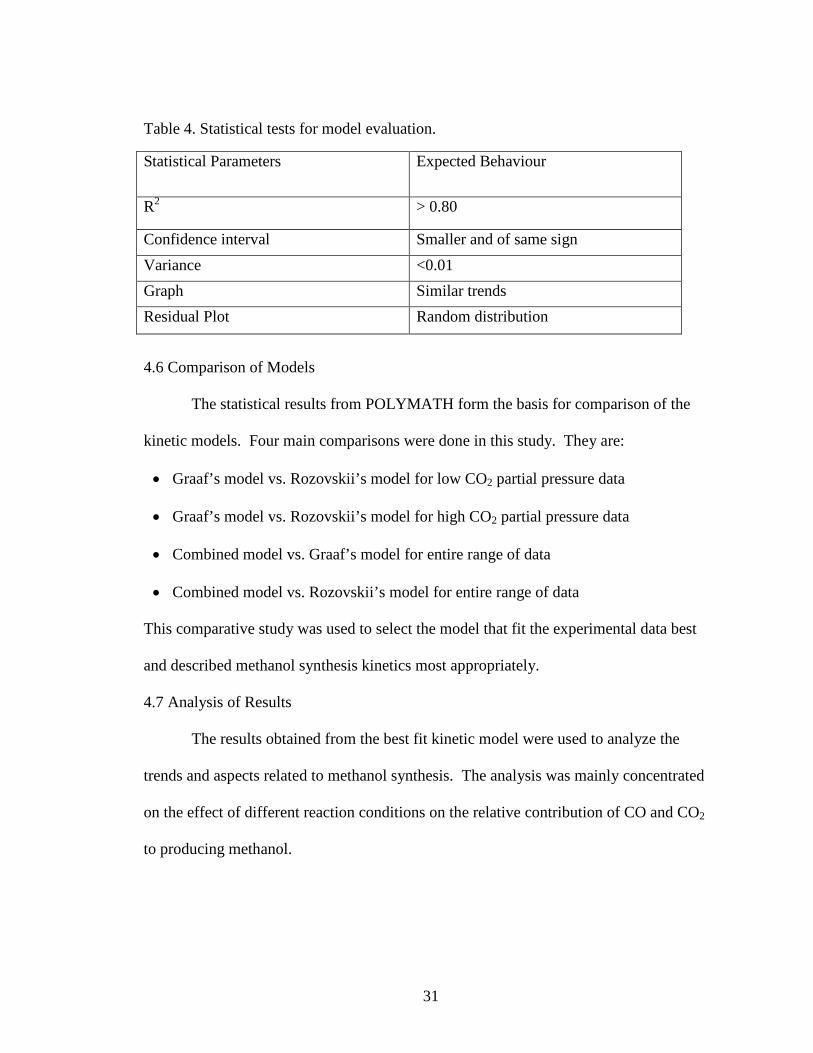
Table 4. Statistical tests for model evaluation.
4.6 Comparison of Models
The statistical results from POLYMATH form the basis for comparison of the
kinetic models. Four main comparisons were done in this study. They are:
• Graaf’s model vs. Rozovskii’s model for low CO2 partial pressure data
• Graaf’s model vs. Rozovskii’s model for high CO2 partial pressure data
• Combined model vs. Graaf’s model for entire range of data
• Combined model vs. Rozovskii’s model for entire range of data
This comparative study was used to select the model that fit the experimental data best
and described methanol synthesis kinetics most appropriately.
4.7 Analysis of Results
The results obtained from the best fit kinetic model were used to analyze the
trends and aspects related to methanol synthesis. The analysis was mainly concentrated
on the effect of different reaction conditions on the relative contribution of CO and CO2
to producing methanol.
Statistical Parameters Expected Behaviour
R2 > 0.80
Confidence interval Smaller and of same sign
Variance <0.01
Graph Similar trends
Residual Plot Random distribution

32
4.8 Summary
Kinetic models proposed by researchers were selected based on their efficacy in
describing methanol synthesis kinetics. Experimental data reported by Calverley after
evaluation was selected for the purpose of modeling. Multiple non linear regression
techniques in POLYMATH were used to fit the models to the experimental data in order
to determine the kinetic parameters and the goodness of fit of the models. Statistical tests
in POLYMATH were used to compare the effectiveness of various models in depicting
kinetics of methanol synthesis and select the best fit kinetic model. The results predicted
by the most appropriate model were used in studying some kinetic features of methanol
synthesis.

33
CHAPTER 5
RESULTS AND DISCUSSION
5.1 Overview
The models were fit to the experimental kinetic data to study their effectiveness in
describing methanol synthesis kinetics. Three different models were compared to select
the best fit model using regression techniques. The results and data generated from the
best fit model were then used to study some trends and kinetic aspects of methanol
synthesis. This chapter includes the following content:
• Regression results and parameter evaluation
• Role of CO/CO2 in producing methanol
5.2 Regression Results and Parameter Evaluation
A wide range of data including both low and high CO2 inlet partial pressures was
chosen for regression so that the applicability of the kinetic models could be validated
properly. The equilibrium constants for CO and CO2 hydrogenation reactions at the
reaction temperature were calculated using the THERMOSOLVER software. They were
found to be 3.88*10-4 for CO hydrogenation and 7.7*10-5 for CO2 hydrogenation
reaction. The equilibrium constants were also calculated using the equations presented
by Graaf et al [36]. The values were found to be very close using the two methods.
The statistical features obtained by fitting Graaf's model to low inlet CO2 partial
pressure data and Rozovskii's model to high inlet CO2 partial pressure data are
summarized in Table 5.

34
Table 5. POLYMATH results of fitting Graaf’s and Rozovskii’s model. Model Parameters
R2 R2adj Variance Rmsd Residuals 95% confidence intervals
Graaf 0.81 0.75 1.9*10-4 0.00323 scattered positive, smaller
Rozovskii 0.91 0.89 4.13*10-5 0.0016 scattered positive, smaller
The statistical features listed in Table 4 are used as indicators of the quality of the
regression models. They are explained below:
• R2 and R2adj were close to one suggesting the models satisfactorily represent the
kinetic data
• Variance and Rmsd was sufficiently small to indicate that both the models represent
the data accurately
• Residuals as shown in Figures B.1 and B.2 in Appendix B were randomly distributed
and did not follow a particular trend signifying the models are statistically
appropriate
• Confidence intervals are listed in polymath reports for both the models shown in
Tables B.1 and B.2 in Appendix B. The models were statistically stable since the
confidence intervals were much smaller than the respective absolute values of the
parameters
The parameter values obtained from the fitting procedure are shown in Table 6.

35
Table 6. Values of kinetic parameters for Graaf’s and Rozovskii’s model.
Model Graaf
Parameter Value k1 ((atm.h)-1) 0.0535 KCO (atm-1) 0.0022 KCO2 (atm-1) 0.0185 Kwh (atm-1) 1011
Rozovskii k3 ((atm.h)-1) 0.0031 K-2 (atm-1) 5.104 K1 (atm-1) 9.978
The graphical representation of the results is shown in Figures 6 and 7.
Figure 6 shows a comparison of experimental values of rate and those calculated from
Graaf's model when the inlet CO2 partial pressures were negligibly small.
0
0.02
0.04
0.06
0.08
0.1
0.12
0 2 4 6 8 10 12 14
data point
met
han
ol p
rod
uct
ion
rat
e (m
ol/g
/h)
r exp
r cal
Figure 6. Comparison of experimental and predicted (by Graaf’s model) methanol production rate.

36
Figure 6 shows that the model proposed by Graaf which was based on CO being
the primary reactant, fit to the data well where CO2 feed partial pressures were very low.
The experimental and estimated rates matched each other quite closely, thereby
confirming the hypothesis. Figure 7 shows a comparison of experimental and calculated
values of rate for Rozovskii's model for high CO2 partial pressure data. The residual
plots for both the regression models are shown in Figures B.1 and B.2 in Appendix B.
Also, the polymath reports summarizing the statistical features of the regression are
shown in Tables B.1 and B.2 in Appendix B.
0
0.01
0.02
0.03
0.04
0.05
0.06
0.07
0.08
0 2 4 6 8 10 12 14
data point
met
han
ol p
rod
uct
ion
rat
e(m
ol/g
/h)
r exp
r cal
Figure 7. Comparison of experimental and predicted (by Rozovskii’s model) methanol production rate.
For CO2 enriched feed, Rozovskii's model that was derived assuming CO2 to be
the main reactant, provided an effective kinetic description of the methanol synthesis

37
process. As shown in Figure 7, the rates estimated from Rozovskii's model are in good
agreement with the experimental rate values.
Both the models were fit to low and high inlet CO2 partial pressure data in order
to compare the effectiveness of each for the given range of data. Figure 8 shows a
comparison of experimental values of rate and those calculated by Graaf's model and
Rozovskii's model when CO2 partial pressures were negligibly small in the feed.
0
0.02
0.04
0.06
0.08
0.1
0.12
1 2 3 4 5 6 7 8 9 10 11 12 13
data point
met
han
ol p
rod
uct
ion
rat
e(m
ol/g
/h)
r exp
r cal GRAAF
r cal ROZOVSKII
Figure 8. Comparison of experimental methanol production rate and those predicted by Graaf’s and Rozovskii’s models at low CO2 inlet partial pressures.
Line column charts have been used to represent the data since it is easier to read
the data with these plots. The trend in Figure 8 on the next page shows that Graaf's
model fit better to the experimental data than Rozovskii's model when CO2 was in
negligible amounts in the feed. Figure 9 shows a comparison of experimental rate values
38
and rate values estimated from Graaf’s and Rozovskii’s models when the CO2 partial
pressures were high in the feed.
0
0.01
0.02
0.03
0.04
0.05
0.06
0.07
0.08
1 2 3 4 5 6 7 8 9 10 11 12
data point
met
han
ol
pro
du
ctio
n r
ate(
mo
l/g
/h)
r exp
r cal ROZOVSKII
r cal GRAAF
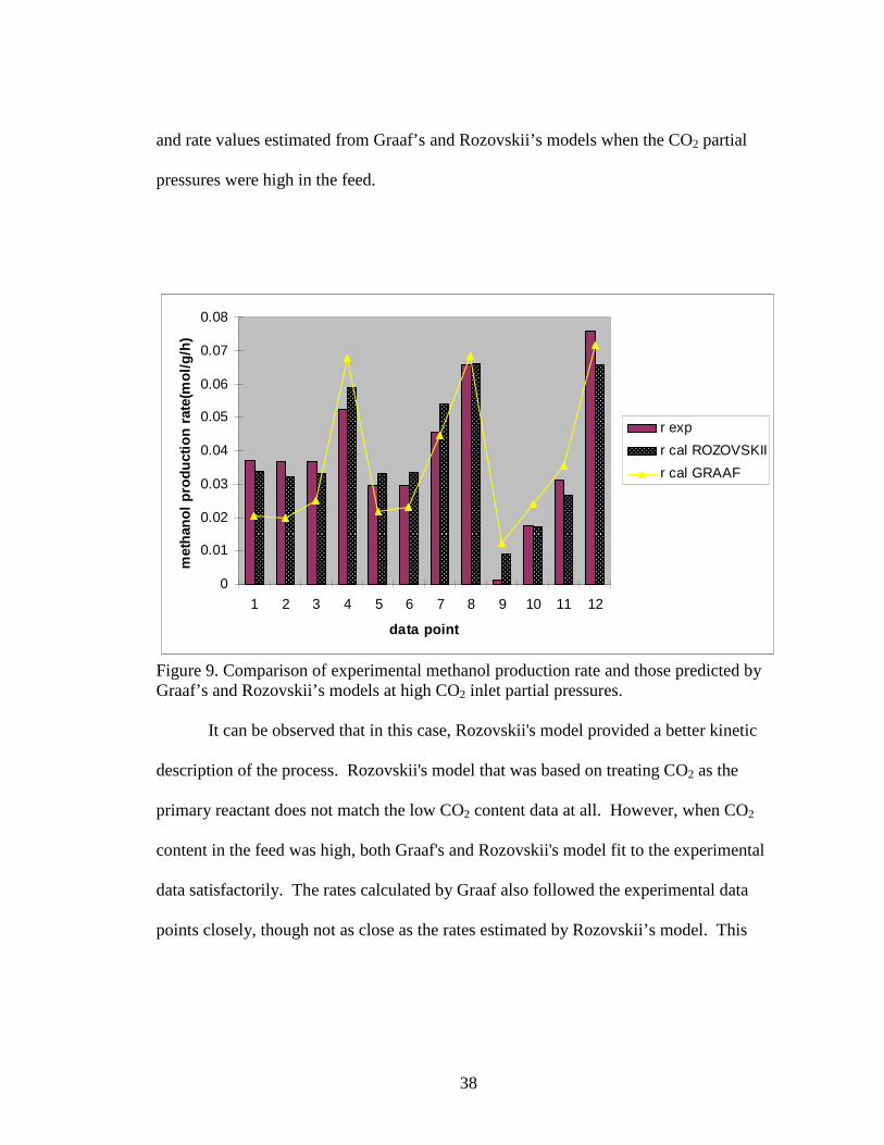
Figure 9. Comparison of experimental methanol production rate and those predicted by Graaf’s and Rozovskii’s models at high CO2 inlet partial pressures.
It can be observed that in this case, Rozovskii's model provided a better kinetic
description of the process. Rozovskii's model that was based on treating CO2 as the
primary reactant does not match the low CO2 content data at all. However, when CO2
content in the feed was high, both Graaf's and Rozovskii's model fit to the experimental
data satisfactorily. The rates calculated by Graaf also followed the experimental data
points closely, though not as close as the rates estimated by Rozovskii’s model. This

39
feature was also observed by Rozovskii in his study. The models proposed by him fit to
the experimental results better when CO2 amounts were higher in the feed [19].
The combined rate expression by summing equations 1and 2 can be written
as,
2
2
2 3 2 2 2
2 2 2 2 2 2 2 2 2
33/2 1/2 31 ,1 ( )
1 1/2 1/22 2 1
(1 )[ / ( )]
(1 )[ ( / ) ] 1 / ( )
m H OH
CO CO H CH OH H eq p m H CO
CO CO CO CO H H O H H O H O H O CO
p pk p
k K f f f f K K p pr
K f K f f K k f K p K p K p− −
−−
= ++ + + + +
Equation (4)
The parameters in this expression were fit to the entire range of experimental data
including low as well as high CO2 inlet partial pressures. Figure 10 shows a comparison
of experimental values of rate and rates estimated form the combined model.
0
0.02
0.04
0.06
0.08
0.1
0.12
0 5 10 15 20 25
data point
met
han
ol p
rod
uct
ion
rat
e (m
ol/g
/h)
r exp
r cal
Figure 10. Comparison of experimental values of methanol production rate and rates estimated form the combined model.
40
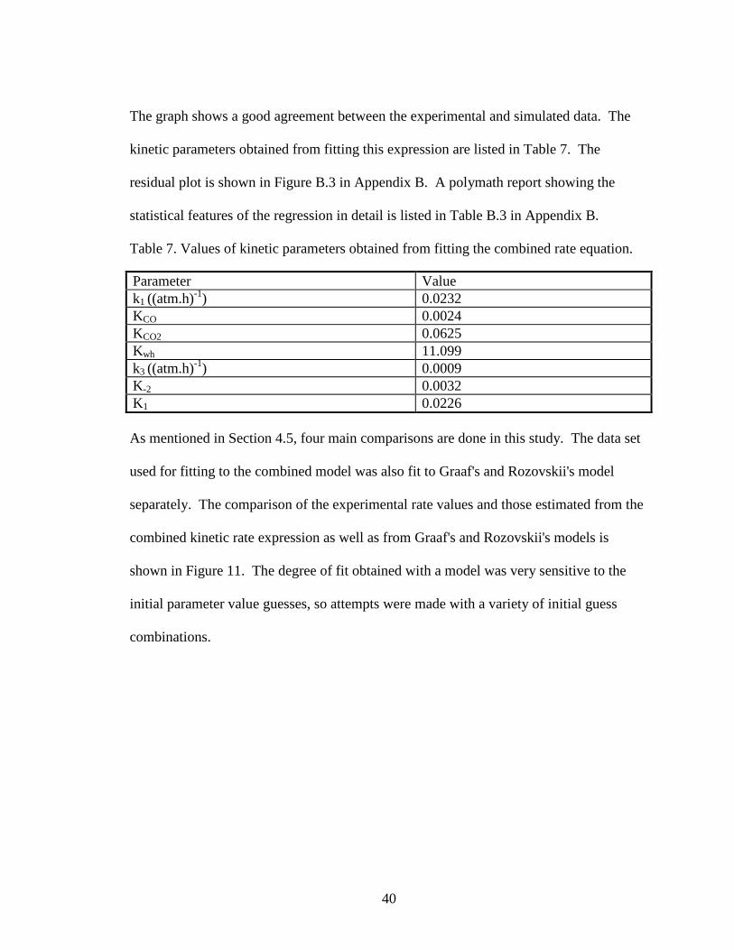
The graph shows a good agreement between the experimental and simulated data. The
kinetic parameters obtained from fitting this expression are listed in Table 7. The
residual plot is shown in Figure B.3 in Appendix B. A polymath report showing the
statistical features of the regression in detail is listed in Table B.3 in Appendix B.
Table 7. Values of kinetic parameters obtained from fitting the combined rate equation.
As mentioned in Section 4.5, four main comparisons are done in this study. The data set
used for fitting to the combined model was also fit to Graaf's and Rozovskii's model
separately. The comparison of the experimental rate values and those estimated from the
combined kinetic rate expression as well as from Graaf's and Rozovskii's models is
shown in Figure 11. The degree of fit obtained with a model was very sensitive to the
initial parameter value guesses, so attempts were made with a variety of initial guess
combinations.
Parameter Value k1 ((atm.h)-1) 0.0232 KCO 0.0024 KCO2 0.0625 Kwh 11.099 k3 ((atm.h)-1) 0.0009 K-2 0.0032 K1 0.0226

41
0
0.02
0.04
0.06
0.08
0.1
0.12
1 2 3 4 5 6 7 8 9 10 11 12 13 14 15 16 17 18 19 20 21
data point
met
han
ol
pro
du
ctio
n r
ate
(mo
l/g
/h)
r exp
r cal COMBINED
r cal GRAAF
r cal ROZOVSKII
Figure 11. Comparison of experimental methanol production rate values and those estimated from the combined kinetic rate expression and Graaf's and Rozovskii's models.
The trend in Figure 11 suggests that the combined rate expression fits to the
experimental data better than the individual models. Although, the rates calculated from
Graaf’s model are also in good agreement with the experimental rate values, it is the
combined rate expression which gives the best results. The results of fitting for the four
comparisons are tabulated in Table 8.

42
Table 8. POLYMATH results of fitting for the comparative study of models.
The statistical parameters listed in Table 8 as well as the trend in Figure 11
indicate that the combined model is the best fit model. Based on the above mentioned
results, it can be concluded that the combined rate expression which includes both CO
and CO2 hydrogenation rate terms describes methanol synthesis kinetics in the best
low CO2 partial pressure Parameter R2 R2adj Variance Rmsd Residuals 95%
confidence intervals
Model
Graaf 0.81 0.75 1.9*10-4 0.00323 scattered positive, smaller
Rozovskii 0.106 -0.67 8.5*10-4 0.0071 follow a trend
positive, smaller
high CO2 partial pressure R2 R2adj Variance Rmsd Residuals 95%
confidence intervals
Graaf 0.71 0.60 1.5*10-4 0.0029 scattered positive, smaller
Rozovskii 0.91 0.89 4.13*10-5 0.0016 scattered positive, smaller
entire range R2 R2adj Variance Rmsd Residuals 95%
confidence intervals
Combined 0.85 0.78 1.6*10-4 0.0022 scattered positive, smaller
Graaf 0.82 0.79 1.5*10-4 0.0024 scattered positive, smaller
entire range R2 R2adj Variance Rmsd Residuals 95%
confidence intervals
Combined 0.85 0.78 1.6*10-4 0.0022 scattered positive, smaller
Rozovskii 0.68 0.64 2.6*10-4 0.0033 scattered positive, smaller

43
possible manner. It was also attempted to fit the combined model separately to low and
high inlet CO2 partial pressure data, however, there were not enough data points in the
two ranges to achieve proper regression results.
5.3 Role of CO/CO2 in Producing Methanol
A number of kinetic models have been proposed in the literature attempting to
describe methanol synthesis kinetics. However, the controversies regarding the carbon
source in methanol and the nature of active sites still remain unsolved. An effort,
therefore, was made in this study to come up with a model that can adequately describe
some features and resolve questions related to methanol synthesis kinetics. The model
proposed in this study is based on the fact that CO and CO2 hydrogenation both
contribute to overall methanol production.
However, the relative contribution of CO and CO2 hydrogenation in producing
methanol cannot be generalized. Instead, the question regarding the main source of
carbon in methanol depends on specific conditions like conversion, pressure, relative
amount of CO and CO2, as well as hydrogen content in the feed. The results have been
discussed under the following conditions:
• Conversion
• Hydrogen content in the feed
• Pressure
• CO/CO2 content in the feed

44
5.3.1 Conversion
Figure 12 shows the Gibb’s free energy change of hydrogenation of CO and CO2
to methanol as a function of temperature. It can be observed that CO2 hydrogenation has
more negative ∆G and thus a higher driving force at very low conversions whereas CO
hydrogenation is more likely to occur at higher conversions at a temperature of 558 K.
Figure 12. Gibb’s free energy change, ∆G, for CO and CO2 hydrogenation to CH3OH and the WGS reaction at P = 75 atm and three different conversion levels as a function of temperature (Reprinted with permission from [34]).
These results from thermodynamics prove that conversion levels can affect the
extent to which CO and CO2 hydrogenation will contribute in producing methanol. We
could not show the same behavior using our results since not enough data points were
available at a constant feed composition and the conversions did not vary much in orders

45
of magnitude. A similar result was reported by Liu et al. in their study in which they
showed that hydrogenation of CO2 was the primary reaction in producing methanol at
low conversion [15].
5.3.2 Hydrogen Content in Feed
Grabow and Mavrikakis have reported that hydrogen content in the feed can have
a marked effect on methanol production rates for CO rich feeds [34]. Methanol
production rate decreases almost linearly with increasing CO2 content in the feed when
the feed is lean in H2 (< 50 %). A similar trend was predicted by our model. Figure 13
shows a plot of methanol synthesis rate and % CO2 in the feed under lean H2 conditions.
0
0.005
0.01
0.015
0.02
0.025
0.03
0.035
0.04
0.045
0.05
0 5 10 15 20 25 30 35
% CO2
met
han
ol p
rod
uct
ion
ra
te (
mo
l/g/h
)
Figure 13. Plot of methanol synthesis rate and % CO2 in the feed under lean H2 conditions.

46
It was observed that the rate decreased linearly as CO2 content in the feed
increased. This behavior can be attributed the fact that hydrogenation of one mole of CO
to methanol needs two moles of H2 compared to CO2 which needs three moles of H2 to
form methanol. Therefore, under lean hydrogen conditions, CO hydrogenation activity is
increased. However, as CO2 % in the feed increased, the overall rate decreased since CO
hydrogenation was inhibited by increased amounts of CO2 in the feed. Also, since there
was no water in the feed in the beginning, CO2 participated competitively in methanol
synthesis as well as RWGS resulting in lower methanol production.
At a pressure of 50 atm, when hydrogen in the feed was increased slightly, the
overall rate showed a maximum value at CO2/(CO+CO2) = 0.036 (encircled in Figure 14)
as predicted by the model developed in this study. Calverley and Smith reported similar
results in their study. However, they observed the maxima when 0.05 <CO2/(CO+CO2) <
0.2 [35]. In our study, hydrogen content in the feed never increased beyond 60%. But at
lower pressures (50 atm in our case), less hydrogen may be needed in the feed for the rate
to increase with increasing CO2 amounts. Figure 14 shows the overall rate plotted as
function of CO2 % at a pressure of 50 atm.

47
0
0.005
0.01
0.015
0.02
0.025
0.03
0.035
0.04
0.045
0.05
0 0.1 0.2 0.3 0.4 0.5 0.6 0.7
CO2/(CO+CO2)
met
han
ol p
rod
uct
ion
rat
e (m
ol/g
/h)
Figure 14. Plot of overall rate as function of % CO2 at a pressure of 50 atm.
Therefore, at 50 atm and H2 content of around 56% in the feed, overall methanol
synthesis rate showed an increase in value as % CO2 increased but it decreased again
possibly due to adsorption of CO2 on active Cu sites necessary for CO activation. This
behavior showing maximum rate a particular value of CO2 % has been reported by other
authors as well like Klier et al. McNeil et al., and Lim et al. [2, 14,and 18].
5.3.3 Pressure
Total pressure also affects the relative contribution from CO and CO2 in
producing methanol. Figure 15 shows the relative contribution of CO and CO2 at a
pressure of 50 atm calculated using the results from our model.
48
0
20
40
60
80
100
120
1 3 5 7 9 11 13 15 17 19 21 23
data point
Rel
ativ
e co
ntr
ibu
tio
n o
f C
O a
nd
CO
2
hyd
rog
enat
ion
(%
)
Rel contribution of CO2
Rel contribution of CO
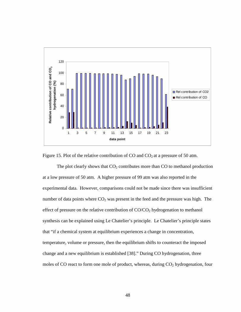
Figure 15. Plot of the relative contribution of CO and CO2 at a pressure of 50 atm.
The plot clearly shows that CO2 contributes more than CO to methanol production
at a low pressure of 50 atm. A higher pressure of 99 atm was also reported in the
experimental data. However, comparisons could not be made since there was insufficient
number of data points where CO2 was present in the feed and the pressure was high. The
effect of pressure on the relative contribution of CO/CO2 hydrogenation to methanol
synthesis can be explained using Le Chatelier’s principle. Le Chatelier’s principle states
that “if a chemical system at equilibrium experiences a change in concentration,
temperature, volume or pressure, then the equilibrium shifts to counteract the imposed
change and a new equilibrium is established [38].” During CO hydrogenation, three
moles of CO react to form one mole of product, whereas, during CO2 hydrogenation, four

49
moles of CO2 react to form two moles of product. When the pressure was high, CO
hydrogenation was favored since it is the pathway which results in lower compression.
5.3.4 CO/CO2 Content in the Feed
Figure 16 shows a comparison between rates calculated from the combined model
and those calculated from the CO hydrogenation model described in the previous sections
when % CO2 in the feed was zero.
0
0.02
0.04
0.06
0.08
0.1
0.12
4 6 8 10 12 14 18 20 22 24 26 28 30
data point
met
han
ol p
rod
uct
ion
rat
e (m
ol/g
/h)
rate from CO hydrogenation
rate from combined model
Figure 16. Plot of rates calculated from combined model and CO hydrogenation model when % CO2 in feed = 0.
The values of rates were quite close to each other suggesting the fact that in the
absence of CO2, the entire methanol was produced entirely from CO. The deviations
could be a result of inadequate fitting of the models.
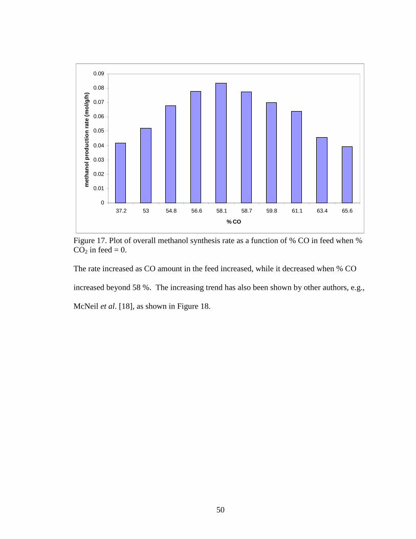
Results obtained from the combined model form the basis of studying a few trends related to methanol synthesis kinetics. Figure 17 shows overall rate plotted as a function of % CO in the feed in the absence of CO2.
50
0
0.01
0.02
0.03
0.04
0.05
0.06
0.07
0.08
0.09
37.2 53 54.8 56.6 58.1 58.7 59.8 61.1 63.4 65.6
% CO
met
han
ol p
rod
uct
ion
rat
e (m
ol/g
/h)
Figure 17. Plot of overall methanol synthesis rate as a function of % CO in feed when % CO2 in feed = 0.
The rate increased as CO amount in the feed increased, while it decreased when % CO
increased beyond 58 %. The increasing trend has also been shown by other authors, e.g.,
McNeil et al. [18], as shown in Figure 18.

51
Figure 18. Predicted (-) compared to experimental (■) methanol production rate versus mole percent carbon monoxide in the feed at 513 K and 2.89/4.38 MPa (Reprinted with permission from [18]).
The decreasing trend can be explained by using the fact that in the absence of
CO2, catalyst deactivation occurs via the Boudouard reaction resulting in carbon
deposition and, therefore, decreasing methanol synthesis rate. The Boudouard reaction
can be written as [39]:
2CO(g) CO2(g) + C(s) Reaction (4)
As amount of CO increased, the reaction proceeded in the forward direction at a faster
rate leading to more carbon deposition and fouling of the catalyst, and therefore, reducing
methanol production rates. The volcanic shape of the plot shown in Figure 17 has also
been reported by Grabow and Mavrikakis [34]. They observed a volcano-shaped curve
when methanol production was plotted as a function of CO2/(CO+CO2) feed ratio for
CO- rich feeds [34].

52
Another trend predicted by our model is that the contribution from CO
hydrogenation to forming methanol decreased as % CO2 increased. The relative
contribution from CO hydrogenation in synthesizing methanol plotted as a function of %
CO2 is shown in Figure 19.
0
5
10
15
20
25
30
35
40
45
0 0.5 1.4 3.1 4.2 6.5 8.8 12.5 14.7 21.8 33
% CO2
con
trib
uti
on
fro
m C
O h
ydro
gen
atio
n
Figure 19. Plot of relative contribution of CO hydrogenation vs. % CO2 in the feed.
The plot shows expected behavior since a high CO2 content can lead to inhibition
of CO hydrogenation due to the strong adsorption of CO2 on active Cu sites necessary for
CO activation.
It has been predicted by our model that the major fraction of methanol resulted
from CO2 hydrogenation, as shown in Figure 20.

53
0
0.01
0.02
0.03
0.04
0.05
0.06
0.07
0.08
0.09
1 3 5 7 9 11 13 15 17 19 21 23 25
data point
met
han
ol p
rod
uct
ion
rat
e (m
ol/g
/h)
rate of COhydrogenation
rate of CO2hydrogenation
Figure 20. Comparison of CO and CO2 hydrogenation rate.
Sahibzada et al. also showed that the intrinsic rate of CO2 hydrogenation was
twenty times faster than CO hydrogenation and at CO2 > 1%, it was the main source of
methanol production [21]. This aspect was also studied by Grabow and Mavrikakis who
showed that larger fraction of methanol was formed from CO2. However, they used a
different feed composition [34].
5.4 Summary
Based on the regression results from POLYMATH, the combined model proposed
in this study was selected to be the best fit kinetic model that describes methanol
synthesis kinetics most appropriately. Predictions from this model have been
successfully used to explain the trends related to methanol synthesis kinetics. It can be
concluded that no generalization can be made regarding the carbon source in methanol.

54
Instead, the relative contribution of CO/CO2 hydrogenation in methanol production
depends on various reaction conditions like conversion, pressure, CO/CO2, and hydrogen
content in the feed. Therefore, experimental data and results should be cautiously
extrapolated and interpreted from low pressure/low conversion laboratory conditions to
high pressure/high conversion industrial conditions.

55
CHAPTER 6
CONCLUSION
This study comprised of investigating various kinetic models proposed in
literature for methanol synthesis and selecting the most appropriate model using
regression techniques. POLYMATH software was the non-linear regression tool used in
fitting different models to published experimental data collected at a temperature of 558
K and pressures of 50 and 100 atm over a Cu/ZnO/Cr2O3 catalyst. The results of fitting
revealed that the combined model including both CO and CO2 hydrogenation rate terms
was the best fit model, thereby confirming the hypothesis made in this research. A
kinetic model like this one that can describe methanol synthesis kinetics satisfactorily can
prove to be very useful in kinetic studies of methanol leading to a better understanding of
the process and improvements in yields and profits.
Kinetic aspects of methanol synthesis, primarily the relative contribution of CO
and CO2 hydrogenation in producing methanol was also studied based on the results
predicted by the best fit kinetic model developed in this work. The results suggest that no
generalization can be made regarding the more dominant reaction pathway. Instead, the
contribution from each hydrogenation pathway depends on reaction conditions like
conversion, pressure, CO/CO2, and hydrogen content in the feed. Methanol production
can be maximized by optimizing these conditions. However, it is recommended to
carefully interpret experimental data and extrapolate results from low pressure/low
conversion laboratory conditions to high pressure/ high conversion industrial conditions
when studying the relative importance of CO2 and CO hydrogenation reactions. Owing

56
to the industrial importance of methanol, there will always be a scope to improve the
productivity of the process. Therefore, further studies should be conducted in order to
reveal more information regarding the kinetic aspects of methanol synthesis.

57
References
1. C.J. Schack, M. A. McNeil and R.G. Rinker, "Methanol synthesis from hydrogen, carbon monoxide, and carbon dioxide over a CuO/ZnO/Al2O3 catalyst: I. Steady-state kinetics experiments," Appl. Catal., 50(1), 247-263 (1989). 2. H.W. Lim, M. Park, S. Kang, H. Chae, J.W. Bae and K. Jun,"Modeling of the kinetics for methanol synthesis using Cu/ZnO/Al2O3/ZrO2 catalyst: Influence of carbon dioxide during hydrogenation," Ind. Eng. Chem. Res., 48(23), 10448-10455 (2009). 3. J. Toyir, P. Piscina, J. Fierro and N. Homs, “Highly effective conversion of CO2 to methanol over supported and promoted copper-based catalysts: influence of support and promoter,” Appl. Catal. B: Environmental, 29, 201-215 (2001). 4. Q. Sun, C. Liu, W. Pan, Q. Zhu and J. Deng, "In situ IR studies on the mechanism of methanol synthesis over an ultrafine Cu/ZnO/Al2O3 catalyst," Appl. Catal., 171(2), 301-308 (1998). 5. T. Fujitani and J. Nakamura, “The chemical modification seen in the Cu/ZnO methanol synthesis catalysts,” Appl. Catal. A: General, 191, 111-129 (2000). 6. X. Liu, G.Q. Lu, Z. Yan and J. Beltramini,"Recent advances in catalysts for methanol synthesis via hydrogenation of CO and CO2," Ind. Eng. Chem. Res., 42(25), 6518-6530 (2003). 7. R. Yang, X. Yu, Y. Zhang, W. Li and N. Tsubaki, “A new method of low-temperature methanol synthesis on Cu/ZnO/Al2O3 catalysts from CO/CO2/H2,” Fuel, 87, 443-450 (2008). 8. Methanol Institute (2009). Methanol production [Online]. Available at http://www.methanol.org/contentIndex.cfm?section=methanol&topic=factSheets&title=Methpr (accessed 1 February 2010). 9. PR Newswire Association (2010). CMIA completes 2010 world methanol cost study [Online]. Available at http://www.prnewswire.com/news-releases/cmai-completes-2010-world-methanol-cost-study-83350592.html (accessed 3 February 2010). 10. M.R. Rahimpour and K. Alizadehhesari, “Enhancement of carbon dioxide removal in a hydrogen-permselective methanol synthesis reactor,” Int J of Hydrogen Energ, 34, 1349-1362 (200
58
11. MIT Technology Review (2006). Methanol: The new hydrogen [Online]. Available at http://www.technologyreview.com/energy/16629/page1/ (accessed 23 January 2010). 12. G. Centi and S. Perathoner, “Opportunities and prospects in the chemical recycling of carbon dioxide to fuels,” Catal. Today, 148, 191-205 (2009). 13. K.M. V. Bussche and G.F. Froment, “A steady-state kinetic model for methanol synthesis and the water gas shift reaction on a commercial Cu/ZnO/Al2O3 catalyst,” J. Catal., 161, 1-10 (1996). 14. K. Klier, V. Chatikavanij, R.G. Herman and G.W. Simmons, “Catalytic synthesis of methanol from CO/H2 : 1V. Effects of carbon dioxide,” J. Catal., 74, 343-360 (1982). 15. G. Liu, D. Willcox, M. Garland and H.H. Kung, “The role of CO2 in methanol synthesis on Cu-Zn Oxide: An isotope labeling study,” J. Catal., 96, 251-260 (1985). 16. G.C. Chinchen, P.J. Denny, D.G. Parker, M.S. Spencer and D.A. Whan, “Mechanism of methanol synthesis from CO2/CO/H2 mixture over copper/zinc oxide/alumina catalysts: Use of 14C-labelled reactants,” Appl. Catal., 30, 333-338 (1987). 17. M. Takagawa and M. Ohsugi, “Study on reaction rates for methanol synthesis from carbon monoxide, carbon dioxide and hydrogen,” J. Catal., 107, 161-172 (1987). 18. M. A. McNeil, C.J. Schack and R.G. Rinker, "Methanol synthesis from hydrogen, carbon monoxide, and carbon dioxide over a CuO/ZnO/Al2O3 catalyst: II. Development of a phenomenological rate expression," Appl. Catal., 50(1), 265-285 (1989). 19. A.Y. Rozovskii and G.I. Lin, “Fundamentals of methanol synthesis and decomposition,” Top Catal., 22 (3-4), 137-150 (2003). 20. S. Fujita, M. Usui, H. Ito and N. Takezawa, “Mechanisms of methanol synthesis from carbon dioxide and from carbon monoxide at atmospheric pressure over Cu/ZnO,” J. Catal., 157, 403-413 (1995). 21. M. Sahibzada, I.S. Metcalfe and D. Chadwick, “Methanol synthesis from CO/CO2/H2 over Cu/ZnO/Al2O3 at differential and finite conversions,” J. Catal., 174, 111-118 (1998). 22. V.E. Ostrovskii, “Mechanisms of methanol synthesis from hydrogen and carbon oxides at Cu-Zn containing catalysts in the context of some fundamental problems of heterogeneous catalysis,” Catal. Today, 77, 141-160 (2002). 23. T.S. Askgaard, J.K. Norskov, C.V. Ovesen and P. Stoltze, “A kinetic model of methanol synthesis,” J. Catal., 156, 229-242 (1995).
59
24. T. Kubota, I. Hayakawa, H. Mabuse, K. Mori, K. Ushikoshi, T. Watanabe and M. Saito, “Kinetic study of methanol synthesis from carbon dioxide and hydrogen,” Appl. Organometal. Chem., 15, 121-126 (2001). 25. A.N. Xin, Z. Yizan, Z. Qiang and W. Jinfu, “Methanol synthesis from CO2 hydrogenation with a Cu/Zn/Al/Zr fibrous catalyst,” Chinese J Chem Eng, 17(1), 88-94 (2009). 26. G.H Graaf, E.J. Stamhuis and A.A.C.M. Beenackers, “Kinetics of low pressure methanol synthesis,” Chem. Eng. Sci., 43(12), 3185-3195 (1988). 27. J.S. Lee, S.H. Han, H.G. Kim, K.H. Lee and Y.G. Kim, “Effects of space velocity on methanol synthesis from CO2/CO/H2 over Cu/ZnO/Al2O3 catalyst,” Korean J. Chem. Eng., 17 (3), 332-336 (2000). 28. V.D. Kuznetsov, F.S Shub and M.I. Temkin. “Kinetics of methanol synthesis and hydrolysis on a copper-containing catalyst,” Kinet Catal +, 25(3), 510-517 (1984). 29. Polymath Software (Date not mentioned) Polymath Help Documentation [Online]. Available at http://www.polymath-softaware.com/PolymathHelp/ (accessed 12 April 2010). 30. H.W. Lim, H. Jun, M. Park, H. Kim, K. Ha, H. Chae, J.W. Bae and K. Jun, “Optimization of methanol synthesis reaction on Cu/ZnO/Al2O3/ZrO2 catalyst using genetic algorithm: Maximization of the synergetic effect by the optimal CO2 fraction,” Korean J. Chem Eng., 27(6), 1760-1767 (2010). 31. G.H Graaf, H. Scholtens, E.J. Stamhuis and A.A.C.M. Beenackers, “Intra-particle diffusion limitations in low pressure methanol synthesis,” Chem. Eng. Sci., 45(4), 773-783 (1990). 32. J.Skryzpek, M. Lachowska and H. Moroz, “Kinetics of methanol synthesis over commercial copper/zinc oxide/alumina catalysts,” Chem. Eng. Sci., 46(11), 2809-2813 (1991). 33. M. Setinc & J. Levec, “Dynamics of a mixed slurry reactor for the three phase methanol synthesis,” Chem. Eng. Sci., 56, 6081-6087 (2001). 34. L.C. Grabow and M. Mavrikakis, “Mechanism of methanol synthesis on Cu through CO2 and CO hydrogenation,” ACS Catal., 1, 365-384 (2011).

60
35. E.M. Calverley, “A study of the mechanism and kinetics of the synthesis of methanol and higher alcohols over alkali promoted copper/zinc-oxide/chromia catalysts,” Open Access Dissertations and Theses, Paper 1913 (1989). 36. G.H. Graaf and A.A.C.M Beenackers, “Comparison of two-phase and three-phase methanol synthesis processes,” Chem Eng Process, 35, 413- 427 (1996). 37. PR Newswire Association (2011). CMIA Completes 2010 World Methanol Analysis [Online]. Available at http://www.prnewswire.com/news-releases/cmai-completes-2011-world-methanol-analysis-105860938.html (accessed 3 November 2011).
38. Wikimedia Foundation Inc. (2011). Le Chatelier’s principle [Online]. Available at en.wikipedia.org/wiki/Le_Chatelier’s_principle (accessed 4 December 2011). 39. Wikimedia Foundation Inc. (2011). Boudouard reaction [Online]. Available at en.wikipedia.org/wiki/Boudouard_reaction (accessed 20 December 2011).

61
Appendix A
ADDITIONAL DATA
The experimental results reported by Calverley are listed in Table A.1. The
reported results included pressure, feed flow rate, catalyst weight, inlet mole fraction for
CO, H2, methanol and CO2 and the outlet mole fraction of methanol for a total of 51 runs.
Table A.1. Experimental results published by Calverley (Reprinted with permission from [35]). Run # Feed
flow rate (mol/h)
Pressure Catalyst mass
Mole fraction in feed exit mole fraction
CO H2 CH3OH CO2 CH3OH
1 1.834 99.7 1.56 0.482 0.312 0.019 0.089 0.0725
2 1.799 99.7 1.56 0.491 0.318 0 0.091 0.0656
3 1.799 99.7 1.56 0.491 0.318 0 0.091 0.0618
4 1.828 99.7 1.56 0.587 0.311 0.019 0 0.0492
5 1.793 99.7 1.56 0.598 0.317 0 0 0.0414
6 2.709 99 1.56 0.581 0.309 0 0 0.03
7 2.709 99 1.56 0.581 0.309 0 0 0.0285
8 2.786 99 1.56 0.566 0.301 0.027 0 0.0455
9 2.786 99 1.56 0.566 0.301 0.027 0 0.0433
10 2.874 99.7 1.56 0.548 0.293 0.053 0 0.0664
11 2.874 99.7 1.56 0.548 0.293 0.053 0 0.0654
12 1.774 99.7 1.56 0.58 0.317 0 0 0.0402

62
Run # Feed
flow rate (mol/h)
Pressure Catalyst mass
Mole fraction in feed exit mole fraction
CO H2 CH3OH CO2 CH3OH
13 1.8 99.7 1.56 0.54 0.323 0 0 0.0607
14 1.833 99.7 1.56 0.53 0.317 0.018 0 0.0673
15 1.81 97.6 1.57 0.57 0.322 0 0.043 0.0415
16 1.807 97.6 1.57 0.419 0.501 0 0.042 0.0586
17 1.805 97.6 1.57 0.611 0.273 0 0 0.0332
18 2.709 99 1.57 0.581 0.309 0 0 0.0306
19 2.714 98.3 1.57 0.583 0.307 0.006 0 0.0329
20 2.786 99 1.57 0.566 0.301 0.027 0 0.0463
21 1.81 98.3 1.57 0.657 0.226 0 0 0.0252
222 1.793 84.7 1.57 0.556 0.32 0 0 0.0308
23 1.839 84.7 1.57 0.407 0.504 0 0 0.0426
24 1.839 84 1.57 0.634 0.227 0 0 0.0192
25 2.412 70.4 1.57 0.656 0.235 0 0 0.0144
26 2.431 70.4 1.57 0.651 0.233 0.008 0 0.0183
27 1.851 98.3 1.56 0.554 0.327 0 0 0.0391
28 1.851 84.7 1.56 0.554 0.327 0 0 0.0296
29 0.959 50 1.56 0.372 0.548 0 0 0.0298
30 0.959 50 1.56 0.372 0.548 0 0 0.0308

63
Run # Feed
flow rate (mol/h)
Pressure Catalyst mass
Mole fraction in feed exit mole fraction
CO H2 CH3OH CO2 CH3OH
31 0.965 50 1.56 0.243 0.558 0 0.147 0.0383
32 0.965 76 1.56 0.243 0.558 0 0.147 0.0787
33 0.965 50 1.56 0.243 0.558 0 0.147 0.0351
34 0.981 50 1.56 0.188 0.553 0 0.218 0.0254
35 1.03 50 1.56 0.283 0.326 0 0.33 0.0127
36 0.964 50 1.56 0.272 0.571 0 0.125 0.0393
37 0.934 50 1.56 0.297 0.57 0 0.088 0.0446
38 0.932 50 1.56 0.297 0.57 0 0.088 0.0432
39 0.937 50 1.56 0.33 0.571 0 0.065 0.0505
40 0.961 50 1.56 0.346 0.557 0 0.049 0.0496
41 0.959 50 1.56 0.362 0.568 0 0.02 0.0532
42 0.949 50 1.56 0.387 0.567 0 0.005 0.0457
43 1.8 99.7 1.56 0.533 0.331 0 0.043 0.0619
44 3.306 50 1.56 0.35 0.561 0 0.028 0.0211
45 3.306 50 1.56 0.165 0.583 0 0.223 0.0102
46 3.306 50 1.56 0.217 0.576 0 0.16 0.0126
47 3.306 50 1.56 0.252 0.578 0 0.119 0.0138
48 3.345 50 1.56 0.342 0.569 0 0.062 0.0182

64
Run # Feed
flow rate (mol/h)
Pressure Catalyst mass
Mole fraction in feed exit mole fraction
CO H2 CH3OH CO2 CH3OH
49 3.421 50 1.56 0.372 0.559 0 0.031 0.0191
50 3.342 50 1.56 0.367 0.569 0 0.014 0.0186
51 3.381 50 1.56 0.382 0.559 0 0 0.0089
The information given in Table A.1 was used to predict the exit gas composition and the
partial pressure of each species using material balance calculations.
The reactor was operated in integral mode during the experiments. Therefore, the
following procedure was used to calculate the rates:
• At a given temperature and pressure, conversion for each run was calculated using
the inlet and outlet composition of reactant, CO. Conversion is calculated using the
following expression:
0
1 AA
A
FX
F= −
where,
XA = conversion
FA0 = inlet molar flow rate of reactant
FA = outlet molar flow rate of reactant
• The ratio of catalyst weight to inlet molar flow rate of CO was also computed
• For a PFR, the rate equation can be written as,

65
0A AA
F dXr
dW− = Equation A.1
or
0
AA
A
dXr
Wd
F
− =
Equation A.2
where,
-rA = rate of reaction
FA0 = inlet molar flow rate of reactant
W = catalyst weight
XA = conversion
• XA was plotted as a function of W/ FA0 and a curve was fit through the points, with
the curve passing through the origin.
• The rates were then calculated by finding the slope of the curve at each data point.
The polynomial function obtained was differentiated to give reaction rates at the
corresponding value of conversion. The plot of XA vs. W/ FA0 is shown in Figure
A.1. As shown in the graph, the curve fits to the data points satisfactorily with an
R2 value of 0.81.

66
y = -0.0008x4 + 0.014x3 - 0.0889x2 + 0.236x - 0.126R2 = 0.8148
0
0.02
0.04
0.06
0.08
0.1
0.12
0.14
0.16
0.18
0 1 2 3 4 5 6 7 8 9
W/FA0
X
Figure A.1 Conversion plotted as a function of W/FA0.
• A fourth order polynomial describes the curve and can be written as
X = -0.0008TF4 + 0.014TF3 - 0.0889TF2 + 0.236TF - 0.126 Equation A.3
TF is the turnover frequency, used interchangeably for W/FA0.
• Differentiating this polynomial, we get
( ) ( ) ( )2 3 0.236 2*0.0889 *TF 3*0.014 *TF – 4*0.0008 *TFdX
dTF= − + Equation A.4
Rates are obtained by finding the above mentioned differential at each value of
conversion. The calculated values of rates are shown in Table 2 in Section 4.2.

67
Appendix B
ADDITIONAL RESULTS
Experimental data including a range of low and high inlet CO2 partial pressures
was used in the regression procedure. The model proposed by Graaf was fit to the low
CO2 inlet partial pressure data and that proposed by Rozovskii was fit to the data with
high CO2 content in the feed. As already explained in Section 4.4, residual plots show
the deviation between the experimental values and the corresponding values calculated
from the models. For a good fit, the residuals should be randomly distributed and not
follow a clear trend around the line of err = 0. The residual plots generated as a result of
fitting Graaf’s and Rozovskii’s models to the kinetic data are shown in Figures B.1 and
B.2.
Figure B.1. Residual plot generated by fitting Graaf’s model to low CO2 inlet partial pressure data.

68
Figure B.2. Residual plot generated by fitting Graaf’s model to low CO2 inlet partial pressure data.
As shown in the Figures B.1 and B.2, the residuals were distributed in a random
manner around the line of err = 0 and did not follow a clear trend indicating the goodness
of fit of the two models. The polymath reports for the same regression models are shown
in Tables B.1 and B.2 displaying the statistical features of the regression.

69
Table B.1. Polymath report generated by fitting Graaf’s model to low CO2 inlet partial pressure data. POLYMATH Report No Title Nonlinear Regression (L-M) 21-Nov-2011
Model: r = (k*Kco*(pco*ph2^1.5-
pm/(ph2^0.5*0.000388)))/((1+Kco*pco+Kco2*pco2)*(ph2^0.5+(Kwh)*ph2o))
Variable Initial guess Value 95% confidence
k 0.1 0.0535024 6.141E-05
Kco 0.01 0.0022467 2.907E-06
Kco2 0.001 0.0184968 0.0066304
Kwh 10. 1011. 4.803157
Nonlinear regression settings
Max # iterations = 64
Precision R^2 0.8149573
R^2adj 0.7532763
Rmsd 0.0032336
Variance 0.0001963
General Sample size 13
Model vars 4
Indep vars 5
Iterations 29
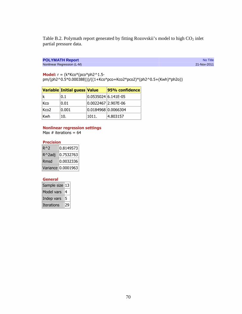
70
Table B.2. Polymath report generated by fitting Rozovskii’s model to high CO2 inlet partial pressure data.
POLYMATH Report No Title Nonlinear Regression (L-M) 21-Nov-2011
Model: r = (k*Kco*(pco*ph2^1.5-
pm/(ph2^0.5*0.000388)))/((1+Kco*pco+Kco2*pco2)*(ph2^0.5+(Kwh)*ph2o))
Variable Initial guess Value 95% confidence
k 0.1 0.0535024 6.141E-05
Kco 0.01 0.0022467 2.907E-06
Kco2 0.001 0.0184968 0.0066304
Kwh 10. 1011. 4.803157
Nonlinear regression settings
Max # iterations = 64
Precision R^2 0.8149573
R^2adj 0.7532763
Rmsd 0.0032336
Variance 0.0001963
General Sample size 13
Model vars 4
Indep vars 5
Iterations 29

71
The residual plot generated as a result of fitting the combined model to the entire range of
data is shown in Figure B.3. The polymath report of the same regression is shown in
Table B.3.
Figure B.3. Residual plot generated by fitting combined model to entire range of kinetic data. The residuals as shown in Figure B.3 are randomly distributed and no clear trend was
observed suggesting the combined model represents the kinetic data appropriately.
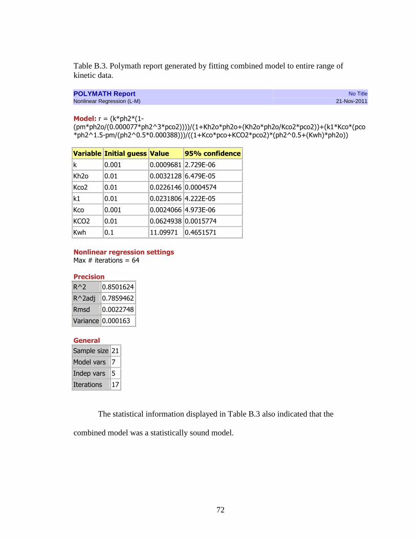
72
Table B.3. Polymath report generated by fitting combined model to entire range of kinetic data. POLYMATH Report No Title Nonlinear Regression (L-M) 21-Nov-2011
Model: r = (k*ph2*(1-
(pm*ph2o/(0.000077*ph2^3*pco2))))/(1+Kh2o*ph2o+(Kh2o*ph2o/Kco2*pco2))+(k1*Kco*(pco*ph2^1.5-pm/(ph2^0.5*0.000388)))/((1+Kco*pco+KCO2*pco2)*(ph2^0.5+(Kwh)*ph2o))
Variable Initial guess Value 95% confidence
k 0.001 0.0009681 2.729E-06
Kh2o 0.01 0.0032128 6.479E-05
Kco2 0.01 0.0226146 0.0004574
k1 0.01 0.0231806 4.222E-05
Kco 0.001 0.0024066 4.973E-06
KCO2 0.01 0.0624938 0.0015774
Kwh 0.1 11.09971 0.4651571
Nonlinear regression settings Max # iterations = 64
Precision R^2 0.8501624
R^2adj 0.7859462
Rmsd 0.0022748
Variance 0.000163
General Sample size 21
Model vars 7
Indep vars 5
Iterations 17
The statistical information displayed in Table B.3 also indicated that the
combined model was a statistically sound model.