kinetic theory of hard spheres - universiteit utrecht
TRANSCRIPT

Journal of Statistical Physics, VoL 21, No. 2, 1979
Kinetic Theory of Hard Spheres
H. van Beijeren 1 and M. H. Ernst 2
Received January 2, I979
Kinetic equations for the hard-sphere system are derived by diagrammatic techniques. A linear equation is obtained for the one-particle-one particle equilibrium time correlation function and a nonlinear equation for the one- particle distribution function in nonequilibrium. Both equations are non- local, noninstantaneous, and extremely complicated. They are valid for general density, since statistical correlations are taken into account system- atically. This method derives several known and new results from a unified point of view. Simple approximations lead to the Boltzmann equation for low densities and to a modified form of the Enskog equation for higher densities.
KEY WORDS: Kinetic theory, linear and nonlinear; hard spheres; equi- librium time correlation functions; diagram expansions; Dyson equation; Enskog equation, modified.
1. I N T R O D U C T I O N
The aim of modern kinetic theory is to derive kinetic equations from first principles, i.e., from Liouville's equation and ensemble theory. The pioneering work in this field has been done by Bogoliubov51~ He starts from the BBGKY hierarchy equations, expressing the time derivatives of the n-particle distribu- tion functions in terms of the (n + 1)-partMe distribution functions. In order to close this set of equations Bogoliubov makes the assumption that, starting from arbitrary initial conditions, after an initial stage of the order of a few mean free times, all n-particle distribution functions become time-independent functionals of the one-particle distribution function. These functionals are obtained in the form of a density expansion, by imposing certain factorization conditions in case the separation between particles is very large. Insertion of
1 Institut ffir theoretische Physik, RWTH Aachen, West Germany. Instituut voor theoretische Fysica, Rijksuniversiteit Utrecht, The Netherlands.
125 0022-4715/79/0800-0125503.00/0 �9 1979 Plenum Publishing Corporation

126 H. van Beijeren and M. H. Ernst
the expression for the two-particle distribution function into the first hierarchy equation yields a closed equation for the one-particle distribution function.
For low densities Bogoliubov's equation reduces to the Boltzmann equation. The first correction term, which involves triple collisions, has been calculated by Choh and Uhlenbeck3 2~ Cohen and Green (a~ have developed the cluster expansion method, in which the functional assumption is avoided. Prigogine and co-workers (4~ independently derived kinetic equations by a different, diagrammatic, method. These were shown to be equivalent to the equations obtained by the cluster expansion method. (5~
In the meantime Green, Kubo, and others developed the correlation function method, (6~ which describes the linear response of a system to a small external disturbance or the decay to equilibrium of a small fluctuation. Both phenomena lead to linear hydrodynamic equations. The transport coefficients in these equations can be expressed as time integrals of equilibrium time correlation functions.
In both approaches to the description of nonequilibrium phenomena two fundamental problems have arisen.
The first problem is that nearly all coefficients in the formal density expansions of the transport coefficients turn out to be divergent integrals. (7~ The cause of these divergences is that the individual terms in the density expansions of the transport coefficients take into account the dynamics of an isolated group of particles only. Within such an isolated group the memory of the initial velocities is not destroyed, so that there are significant contribu- tions to the time correlation functions for all times up to infinity. In reality the memory of the initial velocities is destroyed, or at least distributed over many particles, after a few mean free times, as a result of the frequent collisions suffered by all particles.
The divergences in the density expansions of the transport coefficients can be removed by making resummations in which the many-body character of the dynamics is taken into account. An example is the ring summation of Kawasaki and Oppenheim, (8~ in which the most divergent terms in all orders of the density are summed to finite terms. These terms depend on the density in a nonanalytic way. Hence virial expansions, analogous to the virial expansions of equilibrium quantities, do not exist for transport coefficients.
The second problem is the phenomenon that the time correlation functions occurring in the Green-Kubo formulae do not decay exponentially in time, as was expected previously. Instead they decay as slowly as t -a/2, where d is the dimensionality of the system. This result was obtained first by Alder and Wainwright from computer experiments. (9~ Theoretical explana- tions followed soon, some of them based on hydrodynamical arguments, (~'1~ others derived from kinetic theory. (11~ Especially in two dimensions the long- time tails have dramatic consequences. There, linear transport coefficients

Kinetic Theory of Hard Spheres 127
do not exist, since the time integrals by which they are expressed, according to the Green-Kubo formulas, are divergent. In three dimensions the existence of the Navier-Stokes coefficients is not affected, but there the divergences enter into the Burnett coefficients, (1~ which are transport coefficients appear- ing in the hydrodynamic equations when terms of third order in the gradients of the hydrodynamic densities are taken into account.
The original motivation for the research reported here was a systematic investigation of the density dependence of transport coefficients. Indeed we have been able to renormalize the density expansions of time correlation functions in such a way that the divergences arising from these expansions are removed. This does not mean that we can now present a generalized expansion of transport coefficients in increasing orders in the density, allowing for nonanalytic functions of the density, such as broken powers of n and functions containing logarithms of n. The problem of finding such an expansion is very hard indeed and only little progress has been made beyond the leading nonanalyticity. (12)
On the other hand, the theory developed here turns out to be very useful in the description of long-time tails and the related singularities occurring in the hydrodynamic equations. It provides a derivation for general densities of all results produced by hydrodynamic theories.
Let us briefly sketch the contents of this paper? We derive linear kinetic equations for one-particle equilibrium time correlation functions in the hard- sphere system and a nonlinear kinetic equation for the nonequilibrium one- particle distribution function. The restriction to hard spheres has been made for practical reasons mainly: The dynamics of this system is relatively simple. All collisions are instantaneous, so that interactions between more than two particles do not occur. There exist no bound states between two or more particles, because the interaction is purely repulsive. Finally, all hydrodynamic densities can be expressed as moments of the one-particle distribution func- tion, because the energy density is purely kinetic. Nevertheless, the hard- sphere system shows many of the characteristic features of fluids in general. It is the only model for which a satisfactory kinetic equation at high densities is available (the Enskog equation). Furthermore, it is one of the systems best suited for computer experiments. Therefore it is interesting to have good theoretical predictions just for this model. Extension of the theory developed here to more general potentials is possible, but the technical details become extremely complicated. In our analysis we use a method which was devised by Zwanzig, <14) but is carried much further here. The functions of interest are expanded in infinite series by expressing statistical correlations in terms of Mayer functions and describing the time evolution by means of the binary
3 A more detailed exposition is given {n Ref. 13, to which we will refer for several of the detailed proofs. Copies are available from HvB.

128 H. van Beijeren and M. H. Ernst
collision expansion. The individual terms in this series are represented by diagrams. By a number of subsequent reduction steps the diagrammatic expansions are cast into such a form that well-known diagrammatic methods can be applied. We obtain a Dyson equation for the one-particle-one- particle correlation function, which can be interpreted as a generalized linear Boltzmann equation. In similar way we obtain a nonlinear kinetic equation for the one-particle distribution function. Finally, our equations are re- normalized by standard diagram techniques in order to remove the diver- gences present in the contributions of individual diagrams.
The equations obtained thus are completely general, but they contain a collision operator which is expressed as an infinite sum of diagrams. Hence it is impossible to solve these equations without making further assumptions. An important point, however, is that all statistical correlations are taken into account systematically. Both the Boltzmann equation, valid for low densities, and a modified form of the Enskog equation, which is a good approximation for higher densities, can be extracted by simple approximations.
In the last section a comparison is made with other theories and it is shown how several different results can all be obtained from our equations.
2. E Q U I L I B R I U M T I M E C O R R E L A T I O N F U N C T I O N S FOR THE H A R D - S P H E R E S Y S T E M
W e consider a classical system of identical hard spheres with mass m and diameter a, enclosed in a d-dimensional box of volume V. The Hamil- tonian is given as
N
H(r) = ~ [�89 + V(r~)] + ~ ~(r~) (2.1) i=l
where qb(r)-- ~ if r < cr
(2.2) = 0 if r > ~
The variable P = (N, xl,..., xN) represents the number of particles and their position and velocity coordinates x~ = (r~, v~). The external potential V(r) may contain, besides the wall potential of the box, e.g., gravitational or electrostatic fields. The summation variable a runs over all pairs (i, j ) of different particles in the system and r~ = r~; = r~ - r;.
The dynamics of the system is defined as usual for smooth, hard spheres, where all collisions between pairs of spheres are instantaneous and the motion of a particle between the subsequent collisions is a free motion under the external potential V(r).
We will be interested in equilibrium time correlation functions
(A(P(O))B(P(t)))~q (2.3)

Kinetic Theory of Hard Spheres 129
where A and B are functions of the coordinates of the particles at the initial time and at time t, respectively. The brackets denote an average over the grand canonical ensemble, given by
N
O(P) = (N! ZCr)-~ W(I?) ~ ~b(x3 (2.4) ~ = 1
~b(x) = (/3m/2r exp{- t3[mv2[2 + V(r)]} (2.5a)
W(P)= e x p { - / 9 ~ ~(r~)} (2.5b)
Here p = 1/kBT, where kB is Boltzmann's constant and T is the temperature; the fugacity ~ = (2wm/~h2)a12e ~", where h is Planck's constant and/z is the chemical potential; and the normalization factor Zg~ is the grand canonical partition function. The overlap function W(P) vanishes for all configurations in which two hard spheres overlap each other, and equals unity for all non- overlapping configurations. It can be expanded in a Mayer series as
w ( r ) - - W(h .... , rN)=] - - [ (1 + f , ) = 1 + s ~ f j e + - . - (2.6) a cc cc f l -r162
where the Mayer functions f a r e defined as
with
f~ = 1 - v~(rr - or) (2.7)
~(x) = 1 if x/> 0 (2.8)
= 0 if x < O
We will mainly be interested in the one-particle-one-particle correlation function and the one-particle self-correlation function, which are defined as
F ( x , x ' ; t ) = ( ~ 3 ( x - x , ( O ) ) ( ~ 8 ( x ' - x j ( t ) ) - q ~ ( x ' ) ) ) q (2.9a)
F~(x,x';/)= ( ~ 3(x-x~(O))8(x '-x ,( l)))q (2.9b)
where x' = (r', v'); n(r) is the equilibrium density at position r, and q~(x) is the equilibrium one-particle distribution function
~o(x) = n(r)?o(V) (2.10a)
q~o(V) = (~m/2~r) a/2 exp(- ~mv2 /2 ) (2.10b)
The generalization to n-particle-m-particle correlation functions is discussed in the Appendix.

130 H. van Beijeren and M. H. Ernst
Equilibrium time correlation functions can be rewritten with the aid of unbarred or barred streaming operators ~5) as
<A(F(O))B(F(t))> = .( dr A(P)p(P)S(t)B(F) (2.11a)
= f dr A(F)S(t)p(F)B(F) (2.1 lb)
where ] dF = N ~=o f dxl ... dxu and the operators S and S satisfy the relation
p(F)S(t) = S(t)p(r) (2.12)
Furthermore, they can be expressed in binary collision expansions as
S = S~ + S~ , ~ T~S~ + S~ , ~ T~S~ , ~ T~S~ + ... (2.13a) c~ cr B
= S O + S O �9 ~ T~S ~ + S O �9 ~ T=S ~ �9 ~ TaS ~ + ... (2.13b) tt c~ B
Equation (2.13b) can be obtained from (2.13a) by Hermitian conjugation and subsequent time reversal (see Ref. 15). The asterisk denotes a convolution product. S~ is the N-particle free streaming operator, given by
S~ = exp(L~e~ (2.14a) with
s __ ~ (v~. ~ ~3V(r~) 1 ~ ) (2.14b) = ~ ~r~ ~r~ m
It can be factorized into single-particle operators N
s~ = 1-1 s,~ (ZlS) i = l
These operators generate the free streaming of one particle in the external field V(r) and leave the coordinates of the other particles unchanged.
The binary collision operators T, and T~ are defined (z~ as
lira S~ dd v~(-v,~..a)lv,s.6[ 8(r,j - ~6)[b~(/j') - i] T,j n~o J (2.16a)
T~j = lim ~ a - l [ dO t~(-v,j.~)[v,~.~l{3(r,j - crb)b~(ij) - 3(r,j + ag)}S~ n $ o d (2.16b)
In (2.16a) and (2.16b) the d integration is an angular integration over the d-dimensional unit sphere and the 3 denotes a d-dimensional g-function. The operator b~(ij) transforms the velocities of particles i and j into postcoUisional velocities; its action on an arbitrary function is given by
b~(/j)f(v~, vj, r~, rj,...) = f(vi*, vs*, ri, rj,...) (2.17a)

Kinetic Theory of Hard Spheres 131
with
v~* = v~ - (v~j.~)b, vj* = vj + (vij.~)O (2.17b)
The infinitesimal free streaming operators S~ serve to determine the action of the binary collision operators on functions that are discontinuous at the collision surface, r~ = ~.
Equation (2.15) holds for both forward and backward streaming, i.e., positive (resp. negative) values of t, but (2.16) is valid for forward streaming only. The binary collision operators for backward streaming are given in Ref. 15. In the sequel we will mainly restrict ourselves to the case of forward streaming and indicate when backward streaming is needed. Except for the sign of t in the free streaming operators and the definition of the binary collision operators, the formalisms are completely identical in the two cases.
Besides (2.13a) we will frequently use its Laplace transform
G(z) = G O + G~ ~ T,G ~ + G~ ~ T,~G~ ~ TBG ~ + ... (2.18) ct g B
and a similar form instead of (2.13b). We have omitted the z dependence of G ~ which follows from (2.14) to be given by
G~ = (z - ~ ~ (2.19)
We conclude this section with a list of hard-sphere properties, compiled from Refs. 15, 16, and 13. They are given in Laplace language; their transla- tion into time language is obvious.
f~r~ = T~f~ = 0 (2.20)
f~T B = T~f~ (a ~/3) (2.21a)
f~G ~ + G~ ~ = G~ + G~ ~ (2.22)
) 2 , ) f~, G O + G O f ~ = G~ f~, + G O T~, f ~ G O ~ = i I = i ~ = i
(2.23) T~jf(xk, x~,...) = 0 if k, l,... ~ i, j (2.24)
f dv~ dvj ~jf(x~, xj,...) = f dv~ dvj ~b(x~)4~(xj)~jf(x~, xj .... ) = 0 (2.25)
[if lira f(x~, xj .... ) exists].
3. D I A G R A M M A T I C R E P R E S E N T A T I O N
Insertion of the Mayer expansion (2.6) and the binary collision expansion (2.13a) or (2.13b) into (2.9) and (2.11) yields an expansion of the equilibrium

132 H. van Beijeren and M. H. Ernst
time correlation functions in terms of Mayer functions, free streaming operators, and either T or T operators. The first choice, which corresponds to using (2.11a), forms the most convenient starting point for the unbarred diagram representation; the second choice, corresponding to (2.11b), for the barred representation. In order to make easy contact with existing theories, in Sections 6 and 7, we need the barred representation. In order to stay con- sistently with one representation throughout the paper we always use the barred representation and comment on the unbarred representation in foot- notes. In the barred representation we obtain terms that are typically of the structure
f N (N! Zgr) -1 dx u 8(x - x~) S O * T~S ~ * ,.. TBS~ 1 ~ ~b(x~) 3(x' - xj) i=1
(3.1)
although the final 8-function need not be present, as follows from (2.9a). Expressions of this kind can be represented by diagrams (8'1a'17~ in which
functions and operators are replaced by diagrammatic elements; free stream- ing operators are represented by vertical lines, Mayer functions and binary collision operators by horizontal bonds between the vertical lines, and 3- functions by crosses at the top and bottom of the vertical lines. The same diagrams will be used both in time language and Laplace language.
The relations between diagrams and analytic expressions of the type (3.1) are given in a number of diagram rules (DRs). The first rule describes the elements of which a diagram may consist.
DR 1 (a) An N-particle diagram consists in general of N vertical lines, hori-
zontal bonds, and crosses. Each vertical line represents a particle and is labeled at its top by the number of that particle.
(b) Horizontal bonds are drawn between two vertical lines. A bond will be called an (i, j)-bond, or an a-bond with a = (i, j) , if it connects the lines labeled i and j. There are three different types of horizontal bonds, namely: (i) statistical bonds, representing Mayer functions and drawn as dashed lines (,~--~,); (ii) T-bonds, representing T-operators and drawn as single lines (: :); (iii) T-bonds, representing T-operators and drawn as double lines ( ~ ) . As a general name for T- and T-bonds the term dynamical bond will be used.
(c) A cross at the top or bottom of the line labeled i is called a top-cross or bottom-cross, respectively, and represents a 3-function b ( x - x~) or ~ ( x ' - x , ) .
(d) The leveh, of the dynamical bonds in a diagram, together with the top level and bottom level, where all vertical lines begin (resp. end), are numbered (0, 1, 2,...) from top to bottom. In time language the top level
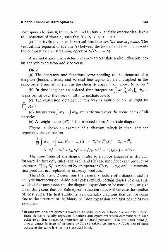
Kinetic Theory of Hard Spheres 133
corresponds to time 0, the bot tom level to time t, and the intermediate levels to a sequence of times t~, such that 0 < tl < t2 < "" < t.
(e) The levels divide each vertical line into vertical line segments. The vertical line segment of the line (i) between the levels l and l + 1 represents the one-particle free streaming operator Si~ +~ - t~).
A second diagram rule determines how to translate a given diagram into an analytic expression and vice versa.
DR 2 (a) The operators and functions corresponding to the elements of a
diagram (bonds, crosses, and vertical line segments) are multiplied in the same order from left to right as the elements appear from above to below. ~
(b) In time language an ordered time integration ft o d h ft~l dt2 fi2 dta ...
is performed over the times of all intermediate levels. (c) The expression obtained in this way is multiplied to the right by
N
NI r i = l
(d) Integrations f dx l ... f dXN are performed over the coordinates of all particles.
(e) A weight factor (N!) -* is attributed to an N-particle diagram.
Figure la shows an example of a diagram, which in time language represents the expression
' f f 5~. dx l ... dx5 ~(x - x l ) S l ~ ... S5 ~ �9 7~2s~ ~ ... s~ ~ �9 T23
• S~ ~ .,. $5 ~ �9 T34S1 ~ ... $5~ 3(x' - x2)r -" r
The translation of the diagram rules to Laplace language is straight- forward. In fact only rules (ld), (le), and (2b) are modified; each product of operators ]--~= z Si ~ is replaced by an operator G~ xN) and all convolu- tion products are replaced by ordinary products.
The DRs 1 and 2 determine the general structure of a diagram and its analytic interpretation. Additional rules exclude certain classes of diagrams, which either never occur in the diagram expansions to be considered, or give a vanishing contribution. Subsequent reduction steps will increase the number of these rules. The first additional rule excludes diagrams that cannot occur due to the structure of the binary collision expansion and that of the Mayer expansion.
4 In case two or more elements stand at the same level or between the same two levels, these elements usually represent functions and operators which commute with each other (e.g., free streaming operators of different particles). The statistical bond fs always comes in front of an operator T~j and behind an operator ~j, if one of these occurs at the same level as the statistical bond.

134 H. van Beijeren and M. H. Ernst
1 2 3
8
4 1 2 3 4
b
I t ~ - - - J
f
Fig. I. (a) A diagram containing all elements defined in DR I, (b) the corresponding cutoff diagram, and (c) the vertices of the latter.
D R 3 (a) There is at most one dynamical bond at each level. (b) There are no dynamical bonds at the top and bot tom levels of a
diagram. (c) Each statistical bond occurs at most once in a diagram.
D R 3a and D R 3b are consequences of the structure of the binary collision expansion (2.13b), and D R 3c follows from the structure of the Mayer expansion (2.6).
The time correlation functions defined in (2.9a) and (2.9b) can now be represented diagrammatically as 5
F(x, x') = [D0(x, x') - Do(x)]/Zgr (3.2a)
F~(x, x') = DoS(X, x')/Zgr (3.2b)
Here Do(x, x') [resp. D0(x)] is the set of all diagrams with one top-cross and one [resp. no] bottom-cross, with only T-bonds as dynamical bonds, and with statistical bonds only at the bot tom level, satisfying DRs 1-3. 6 DoS(x, x') is the subset of all diagrams belonging to Do(x, x') where the top-cross and the bottom-cross are attached to the same vertical line.
Two other definitions will be needed frequently:
A vertex is a set of bonds and/or a cross located at one level of a diagram, together with the entries and exits of attached vertical lines. At each level of a diagram a vertex is present, containing all bonds and/or crosses at that level.
The vertical line length of a diagram is the total number of its vertical line segments. For example, the vertical line length of Fig. la is 16.
5 The bar indicates the barred representation. 6 In the unbarred representation one has sets Do(x, x'), Do(x), and DoS(x, x'), which
have only T-bonds as dynamical bonds and statistical bonds only at the top level.

Kinetic Theory of Hard Spheres 135
A first simplification of diagrams is obtained by the introduction of two cutoff rules, giving prescriptions to delete vertical line segments corresponding to operators which may be omitted without affecting the value of the diagrams. These rules are given together:
DR 4a (4b). Each vertical line is deleted above (below) the highest (lowest) level where a vertex is attached to it. This level is called the upper
(lower) cutoff level of the line. The integrations f dx~ are shifted from the top
level to the upper cutoff levels of the vertical lines. The factors ~b(x~) are shifted from the bottom level to the lower cutoff levels.
Let us consider the consequences of these rules. If a vertex is attached at the top or bottom of a vertical line, clearly nothing of this line is deleted at the upper [resp. the lower] end. The upper and lower cutoff levels of a line may coincide, so that the line is reduced to a single point. If no crosses or bonds are attached to a line, it is deleted completely, although its label is maintained. The cutoff rules do not change the value of a diagram, as can be seen from the relations
S~~ = ~b(xOS~~ (3.3)
f dx~S~~ .... ) = f dx~f (x~ ,x , .... ) (3.4a)
S~~ x~,...) = f ( x t, xk .... ), j , k .... r i (3.4b)
If so desired, cutoff diagrams may always be replaced by the original diagrams again.
Figure lb shows the diagram of Fig. la after application of the cutoff rules. In Laplace language the corresponding analytic expression is
x f dxa T2aa~ dx~ r3~r162176 ~(x' - x~)r
The vertical line length of this diagram has been reduced to 8. Its vertices take the form shown in Fig. lc.
By virtue of the cutoff rules a further simplification can be obtained by translating (2.24) and (2.25) into a diagram rule:
DR 5a (5b). From each T-bond (T-bond) at least one vertical line runs downward (upward).
This DR yields the first example of diagrams that are excluded since they give vanishing contributions. The optimal profit of this DR will only be obtained after the application of certain reductions, to be defined later.

136 H. van Beijeren and M. H. Ernst
The time correlation functions F and F ~ can now be expressed as
F(x, x') = [/~l(x, x') - D~(x)]/Zgr (3.5a)
FS(x, x ' ) ~- DiS(x, xt) /Zg r ( 3 . 5 b )
where D1 a n d / ~ s are obtained from Do and/?0 ~ by applying the cutoff rules and DR 5. Hence these sets can be defined by replacing " D R s 1-3" in the definition of Do by " D R s 1-5."
An important simplification is obtained by expressing the time correla- tion functions in terms of linked diagrams. A diagram is linked (18) if there is a path consisting of bonds and vertical line segments between any two particles. It is unlinked otherwise. Some examples are given in Fig. 2.
An unlinked N-particle diagram consists of a number of pieces which are linked by themselves, but which are not linked to each other. The piece containing the top-cross will be called reference piece, and contains, say, s particles; the remaining part of the diagram, containing N - s particles, is called the disjoint part and may consist of several disjoint pieces. Before collecting diagrams with the same reference piece we first relabel all particles in natural order: in the reference piece as 1, 2,..., s, and in the disjoint part as s + 1,..., N. After this relabeling each N-particle diagram with an s-particle reference piece occurs N!/[(N - s)! s!] times. Its total contribution is simply
[N!/(N - s)! s!](N[) -1 f dxz ... dxs f dx~+~ ... dXN "', on the product of the
contribution of the reference piece and that of the disjoint part, both inter- preted as" independent" diagrams with weight factors (s !) - 1 and [(N - s)!]-1, respectively, according to DR 2e.
Hence all diagrams contributing to a correlation function as given by (2.9)-(2.11) and having the same reference piece, say D, can be added up and their sum can be represented by D, provided its contribution is multiplied by an extra factor representing the sum of all possible disjoint parts. In Ref. 13 it is shown that this factor is Zgr for linked diagrams containing both a top- and a bottom-cross. It is also cross give no contribution to
1 2 3 1 2 1 2 3
a ~ ~ ' - - - b J ( - - - - - "* c
2 3
proven that linked diagrams without a bottom- the time correlation functions. This is the result
2 3
e
Fig. 2. Examples of linked diagrams (a and b) and unlinked diagrams (c, d, and e).

Kinetic Theory of Hard Spheres 137
of a cancellation between diagrams in which the bottom-cross occurs in a disjoint piece and diagrams without a bottom-cross, representing the sub- tracted te rm/ ) l (x ) on the right-hand side of (3.5a). As a result a diagram rule can be added:
DR 6. All diagrams are linked.
Now the time correlation functions occurring in (2.9)-(2.10) can be expressed in terms of linked diagrams as 7
F(x, x') = Co(x, x') (3.6a)
FS(x, x') = CoS(x, x') (3.6b)
Here Co(x, x') [resp. CoS(x, x')] is the subset of all linked diagrams belonging t o / ) l ( x , x') [resp./51'(x, x')].
4. S H I F T I N G P R O C E D U R E
The next step in the reduction of the diagrammatic expansions (3.6) is a redistribution of statistical bonds over the different levels of the diagrams, called the shifting procedure. This can in principle be achieved by commuting free streaming operators and/or dynamical bonds with statistical bonds according to Eqs. (2.20)-(2.23). As a result of the shifting procedure the statistical correlations between particles are taken into account at more relevant times than before. This simplifies the calculation of several contribut- ing diagrams considerably (see Fig. 3 for an example). Furthermore, thanks to the shifting procedure, the structure of the diagrams becomes more sym- metric, in the sense that the same elements can in principle occur everywhere (before, statistical bonds could only occur at the bottom level). This enables one to apply standard field-theoretic methods, such as the Dyson equation and the skeleton renormalization. The Dyson equation in this case becomes a kinetic equation, or generalized Boltzmann equation, for the one-particle- one-particle correlation function. In the high-density regime a generalization of the linearized Enskog equation comes out in a natural way as the simplest approximation to this equation. The skeleton renormalization removes the divergences occurring in a straightforward density expansion of the general- ized Boltzmann collision operator. Furthermore, the same procedure can be used to derive nonlinear kinetic equations for the n-particle distribution functions, which will be discussed to some extent in Section 8. In the high- density regime a generalization of the nonlinear Enskog equation is obtained
7 Starting from the unbarred representation one obtains sets Co(x, x') and CoS(X, x') which are related to the sets Do and Do' in the same way that Co and Co' are related to /)o and /)o ~.

138 H. van Beijeren and M. H. Ernst
1 2 3 4 1 2 3 4
[ l i
a b
Fig. 3. Two similar diagrams in which statistical correlations are taken into account at different times.
as the simplest approximation to the kinetic equation for the one-particle distribution function.
The actual shifting procedure amounts to a systematic repeated applica- tion of (2.22)-(2.23) to diagrams of the sets Co and Co g , defined beneath (3.6). A simple example is given in Fig. 4. The details are given in Ref. 13 ; here we restrict ourselves to a description of the leading principles for the shifting procedure and we describe the sets of diagrams resulting when the shifting procedure is applied to the sets Co(x, x') and CoS(X, x').
We need the concepts of line reducibility and articulation lines, which are defined as follows:
A line-irreducible diagram is a diagram that contains no articulation lines.
A vertical line in a diagram is an articulation line if deletion of this line and all bonds and crosses attached to it produces an unlinked diagram. 8 A line-reducible diagram is a diagram that contains at least one articulation line,
I t is always possible to decompose a line-reducible diagram into a number of line-irreducible diagrams by cutting it along all its articulation lines. In this process top- and bottom-crosses are omitted, as well as all levels where vertices of different star factors were attached. Next the cutoff rules
Articulation lines are similar to articulation points in graph theory. (19) If all vertical lines in a diagram are contracted'to points, articulation lines become articulation points in the resulting graph.
1 2 ;3 1 2 3 1 2 3
Fig. 4. Example of shifting in a diagram.
1 2 b
H

Kinetic Theory of Hard Spheres 139
are applied to all lines, according to DR 4. In analogy to the terminology used for Mayer graphs, the line-irreducible diagrams into which a line-reducible diagram can be decomposed will be called the star factors of that diagram.
The aim of the shifting procedure is to give the diagrams a maximally compact structure, such that:
(a) The vertical line length (defined at the end of Section 3) of each star factor of the diagram is minimal; this means that it cannot be decreased by moving statistical bonds to different levels, keeping the positions of all dynamical bonds fixed.
(b) Each statistical bond stands at the lowest possible level of the complete diagram that is compatible with the requirement of minimal line length of the individual star factors.
In Ref. 13 it is proven that these two requirements determine the shifting procedure completely. 9
The first implication of these requirements is that star factors consisting of statistical bonds only remain at the bot tom level of the diagram. Next, if statistical bonds are shifted to the lowest possible levels, compatible with minimal line length, the set of diagrams Co(x, x ') is transformed into a new set Cl(x, x'), which consists of all linked barred regular diagrams with one top-cross and one bot tom-cross? ~ A diagram is called barred regular if every vertex in any star factor of the diagram is a barred regular vertex, a concept defined below:
A barred regular vertex v at a level l in a star factor A of a diagram D has the following properties:
(i) The vertical line length of A increases if any nonempty set of statistical bonds belonging to v is moved to the level 1 + 1, unless I is the bot tom level.
(ii) The vertical line length of A does not decrease if any set of statistical bonds belonging to v is moved to the level l - 1. (4.1)
(iii) I f v contains a dynamical bond, this is a T-bond if in A more lines run upward than downward from the vertex; it is a T-bond otherwise.
(iv) v does not contain bondsf~ and T~ or T~ with equal c~.
9 The requirement (a) of maximal compactness of the star factors by itself is not sufficient to determine the shifting rules uniquely. Therefore (b) has been added, although this requirement is not free of arbitrariness. For example, an alternative to (b) is the requirement that each statistical bond stands at the highest possible level, compatible with minimal line length. This gives rise to the regular representation. It is worth noting that both regular and barred regular representations can be obtained by applying the shifting rules either to the sets Co and Co s or to the equivalent sets Co and Co ~.
lo When taking the alternative option of shifting statistical bonds to the highest possible levels, compatible with the requirement of minimal line length, one obtains the set C~(x, x') of so-called regular diagrams.

140 H. van Beijeren and M. H. Ernst
1 2 3 1 2 2 3
a b c
Fig. 5. (a) A line-reducible diagram and (b, c) the star factors of which it consists.
Property (iv) excludes diagrams that give vanishing contributions as a consequence of the relations (2.20), f~T~ = T~f~ = O.
Note that a vertex in a line-reducible diagram need not satisfy properties (i)-(iv) with respect to the complete diagram. For instance, in Fig. 5a the T12-bond is a regular vertex; it satisfies all properties (i)-(iv) with respect to the star factor to which it belongs (Fig. 5b). Nevertheless it does not satisfy property (iii) with respect to the complete diagram.
As a consequence of (3.6), the functions F(x, x') and FS(x, x') can be expressed as
F(x, x') = CI(x, x') (4.2a)
F~(x, x') = C~(x, x') (4.2b)
where C1 ~ is the subset of all diagrams of C1 where the top-cross and the bottom-cross are attached to the same vertical line.
Some examples of vertices are shown in Fig. 6. The vertices in Figs. 6a-c are barred regular; the others are not, because they violate property (i) (Figs. 6d, f, g) or (ii) (Fig. 6e) or (iii) (Fig. 6h).
Finally, in Fig. 7 some diagrams are shown which belong to the set C~(x, x').
t~7-; : - , U..z._'-_~ k--,_._ T . . . . J a b c
d e f
k=z~----~ I l U-a--- "-t g h i
Fig. 6. Examples of vertices.

Kinetic Theory of Hard Spheres 141
I I 2 1 2 3 4 I 2 3
a b c d
Fig. 7. Some diagrams belonging to the set Cl(x, x').
5. U N L A B E L E D D I A G R A M S , E L I M I N A T I O N OF THE F U G A C I T Y
We take together all sets of diagrams that can be transformed into each other by permutations of particle labels and represent such sets by unlabeled diagrams. In the following reduction the fugacity is eliminated in favor of the density. This section is concluded by a review of the diagram rules as applicable after these reductions.
Diagrams that can be transformed into each other by a mere permutation of particle labels have equal values, since in the corresponding analytic expressions the integrations over all corresponding particle coordinates are performed. Hence one may take together the sets of all diagrams that can be transformed into each other by such permutations and represent each set by an unlabeled diagram, c18~ Its value is obtained as the value of a corresponding labeled diagram times the number of such diagrams. For an N-particle dia- gram this number is N! divided by a symmetry number s; this is the number of permutations of particle labels leaving the labeled diagrams unchanged. On replacement of labeled by unlabeled diagrams the factor (N!)-1 in DR 2e must accordingly be replaced by 1/s. An example of a diagram with symmetry number larger than l is given in Fig. 8. This diagram is invariant under the permutation of particles 2 and 3 and that of particles 5 and 6. Hence it has symmetry number 4.
In the next reduction step the fugacity is eliminated in favor of the density. To this end consider the topological structure of barred regular diagrams. There exist barred regular diagrams from which a piece without any top- or bottom-crosses can be removed by a single cut either through a
3 2 ! 4 5 6
Fig. 8. A diagram with symmetry number s = 4.

142 H. van Beijeren and M. H. Ernst
.__J L
a b c
* [ I L I.
l . . . �9 - ~. ~I..- --,.X - - - - I ~ - - - - , ~
e f
I----'I~--4 I d
Fig. 9. (a) A diagram with dynamical articulation points and (b) its trunk; (c, e) two diagrams with statistical articulation points and (d, f) their trunks.
vertical line segment or through a point of a Mayer graph at the bottom. The cut point will be called a dynamical or a statistical articulation point, (19)'11 respectively, and the cutoff piece without crosses will be called, respectively, a dynamical or a statistical branch. A diagram without branches will be called a trunk diagram; the trunk of a diagram is obtained by deleting all of its branches. Some examples of diagrams containing articulation points and the corresponding trunks are shown in Fig. 9. Notice that the trunk of a barred regular diagram is always barred regular, since the trunk and the branches of a diagram consist of completely different star factors.
Barred regular diagrams with branches extending above the correspond- ing articulation points are forbidden by DR 5a. Consequently, dynamical branches in barred regular diagrams are always attached from below, as in Fig. 9a, and statistical branches cannot contain dynamical bonds. Examples of diagrams excluded by DR 5b are shown in Fig. 10.
11 Articulation points must be well distinguished from articulation lines. Indeed, vertical lines containing an articulation point are always articulation lines, but an articulation line need not contain an articulation point.
h a
+N I__J-
C Fig. 10. Diagrams forbidden by DR 5b.

Kinetic Theory of Hard Spheres 143
All barred regular diagrams can be obtained from barred regular trunk diagrams by attaching branches at the lower cutoff levels of the vertical lines, as defined in DR 4. Consider first the case where a cutoff level is different from the bottom level. Suppose this level corresponds to a time h- Then the set of all barred regular branches that can be attached at this lower cutoff point just represents the one-particle distribution function
~ dx2 ... dxN S(t - h)p(x, x2 .... , x~) ff'~=l d
Here x is the phase of the particle to which the line containing the cutoff point corresponds, and p again is the grand canonical density. One can under- stand this by making a diagram expansion of the expression above (with a top-cross representing the nonintegration over x) and applying all the reduction steps described so far. The operator S(t - h) may be replaced by unity, since it leaves the grand canonical density unchanged. Then the integrations over x2,..., xN and the summation over N can be performed, yielding the equilibrium one-particle distribution function 9(x) defined by (2.10).
On the other hand, the set of all statistical branches that can be attached to the kth particle at the bottom of a trunk diagram represents just the fugacity expansion of the one-particle distribution function q~(x). Hence the summation over these branches replaces the fugacity ~b(x~) [defined in (2.5)] of the bottom particles in a trunk diagram by the local density q~(xk) at their final position xk.
The net result of the preceding reduction can be expressed in a new diagram rule:
DR 7. All diagrams are trunk diagrams [if in DRs 2c and 4, ~b(x~) is replaced by q~(x~)]. 12
In Section 4, below the definition of a barred regular vertex, we stated that such a vertex may dissatisfy the set of properties (i)-(iv) of (4. I) with respect to the complete diagram, and in Fig. 5 an example was given where this happened. It is important to notice here that after the reduction to trunk diagrams this can no longer occur. Hence a vertex satisfying requirements (i)-(iv) of (4.1) with respect to the complete diagram to which it belongs is barred regular and vice versa. A proof of this is given in Appendix C of Ref. 13.
12 It is to be noted, however, that after the reduction to trunk diagrams the replacement of cutoff diagrams by the corresponding noncutoff diagrams in general is no longer allowed. The reason is that usually &0 and 9(x0 do not commute. An important exception is the case that no external potentials are present.

144 H. van Beijeren and M. H. Ernst
As a conclusion of this section the diagram rules are summarized in a concise formulation. They are denoted with an asterisk to distinguish them from the original rules. Concepts like statistical bonds, vertical lines, linked diagrams, and barred regular vertices have been defined in Sections 3-5. The first six diagram rules describe the structure of diagrams, the last rules describe their analytic interpretation. The rules are given here in time language the translation to Laplace language is obvious.
DR 1' . All diagrams consist in general of vertical lines, statistical bonds, T-bonds, T-bonds, and a top- and bottom-cross.
DR 2*. All diagrams are linked (see Section 3). DR 3a*(3b*). Each vertical line is deleted above (below) the highest
(lowest) level where a vertex is attached to it. DR 4a*(4b*). From each T-bond (T-bond) at least one line runs
upward (downward). DR fi*. All diagrams are trunk diagrams. DR 6". All vertices are barred regular (see Section 4). DR 7*. The levels of a diagram correspond to an ordered set of times
0 < tl < t2.." < t ,_ l < t, and each vertical line segment represents a free streaming operator of the corresponding particle, between the two times corresponding to the top and bottom of the line segment.
DR 8*. The order of elements in a diagram from top to bottom is the same as the order of corresponding operators and functions from left to right in the analytic expression represented by the diagram.
DR 9*. Factors q~(x~) have to be added at the lower cutoff levels of the vertical lines.
DR 10". Integrations over the phases x~ of all particles must be per- formed at the times corresponding to the upper cutoff levels of the vertical lines.
DR 11". Time-ordered integrations must be performed over the times tl,..., t~_~ corresponding to the intermediate levels.
DR 12". Labeled diagrams have a weight factor (N!)- 1, where N is the number of particles in the diagram; unlabeled diagrams have a weight factor l/s, where s is the symmetry number of the diagram.
The function F(x, x') can now be expressed at
F(x, x') = C2(x, x') (5.1)
where C2(x, x') is the set of all diagrams satisfying DRs 1"-12". In similar way FS(x, x') can be identified with a set C2S(x, x').

Kinetic Theory of Hard Spheres 145
6. D Y S O N E Q U A T I O N
In this section kinetic equations for the functions F(x, x') and FS(x, x') will be derived. They can be interpreted as kernels of integral operators or one-particle propagators r(x, t) and rS(x, t), which act on arbitrary functions A(x) of the one-particle phase x, i.e.,
f '. t)A(x') P(x, t)~(x)A(x) (6.1) dx' F(x, x , =
and a similar definition for r ~ in terms of F ~, which will be postponed until the end of this section. An equivalent form of (6.1) is
F(x, x' ; t) = .I dxl 3(x - x l )P(x l , t )q~(xl) 3(x' - xl) (6.2)
The propagator F can, of course, also be represented by the set of diagrams C2(x, x'), provided the meaning of the top- and bottom-crosses is slightly changed: It follows from (6.1) and (6.2) that (i) one should not integrate over the phase x of the top-cross particle, and (ii) a bottom-cross on the line of, say, particle j represents now the permutation operator Pxlxj, which inter- changes xl and xj. In addition, one should remove the factor ~ (x j )= Px~x?(xl) at the bottom level of this line.
The diagrams contributing to P can be distinguished into diagrams with and without statistical vertices. A statistical vertex contains no dynamical bonds and at least one statistical bond. It can occur only at the bottom of a diagram. The set consisting of all diagrams of P without statistical vertices will be denoted by r D. We first consider the diagrams of F with statistical vertices. If a diagram of r contains a statistical vertex at the bottom, there is exactly one line running upward from it, since the diagram is barred regular. Let the particle corresponding to this line be i. Then i is not the bottom-cross particle, because statistical articulation points are forbidden by DR 5*. If the bottom-cross is attached to particle j, the statistical vertex connecting i and j may be any connected Mayer graph with i a n d j as root points, (~9~ but without statistical articulation points. Hence the sum of all allowed statistical vertices at the bottom of diagrams contributing to 1~, represents the pair correlation function ~
G(ri, rj) = n2(r~, rj) n(r~)n(rh 1 (6.3)
where n2 is the equilibrium pair distribution function. Furthermore, if one removes the statistical vertex at the bottom, the remaining diagram may be any diagram contributing to r ~ Hence the complete propagator I~ can be expressed as
r(x~, t ) = P~(x~,t)[l+fdx2G(r~,r2)Px~(x2)] (6.4)

146 H. van Beijeren and M. H. Ernst
u
tz
d
h
Fig. 11. Some diagrams contributing to/~.
Consider next the operator fib. The simplest diagram contributing to F~ is the free propagator. Then there are diagrams containing one bubble; in these diagrams a free propagator is running down from the top-cross to a bubble and another free propagator is running down from this bubble to the bottom-cross. A bubble or collision diagram ~a is a linked diagram without statistical vertices and is characterized by the property that it cannot be separated into two disjoint parts by a single cut through a vertical line. The top and bottom of a bubble consist of a vertex (which may be the same one). An entry at the top-vertex and an exit at the bottom-vertex of the bubble mark the places where free propagators are attached in the complete diagram of which the bubble is a part. Examples of bubbles are shown in Fig. 11. The entries and exits are marked by crosses, which have the inter- pretation discussed at the beginning of this section.
The interpretation of collision diagrams is given by DRs 7"-12", provided one keeps in mind that crosses are interpreted as described at the beginning of this section and that in time language the contributions of instantaneous diagrams, i.e., diagrams containing no vertical line segments,
must be multiplied by a factor 3+(t) defined by fo dt f( t ) 3+(t) = f+(0).
This is most easily understood by transforming back from Laplace language. The binary collision operator is z independent, hence its inverse Laplace transform contains a 3+-function of the time.
The barred regular collision operator B(xl) is now defined as the sum of all barred regular collision diagrams? 4 As short-hand notations we will use B~ or B. Besides the free propagator and the one-bubble diagrams, the propagator contains two-bubble diagrams, three-bubble diagrams, etc., con-
la Collision diagrams correspond to self-energy diagrams in field theory. (le) 14 Similarly one can define a regular collision operator B(xl) as the sum of all regular
collision diagrams. B(xl) is not equal to/~(xl).
Kinetic Theory of Hard Spheres 147
I j i a b c
Fig. 12. A few diagrams contributing to ~D.
sisting of an alternating chain of free propagators and bubbles, but always beginning and ending with a free propagator. All these diagrams have the convolution property, i.e., their contribution is the convolution product of the contributions of the subsequent constituent free propagators and bubbles, provided one uses unlabeled diagrams; for only in that case does the weight factor of a complete diagram factorize into the product of the weight factors of the constituent pieces. In Laplace language the convolution property becomes an ordinary product property.
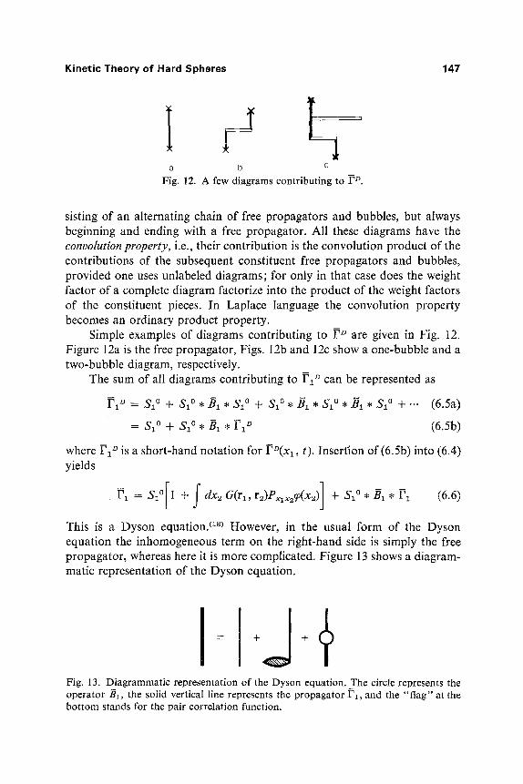
Simple examples of diagrams contributing to r ~ are given in Fig. 12. Figure 12a is the free propagator, Figs. 12b and 12c show a one-bubble and a two-bubble diagram, respectively.
The sum of all diagrams contributing to 1~ ~ can be represented as
F1D = $1 ~ + 5'1 ~ �9 �9 $1 ~ + S~ ~ �9 B~ �9 5'1 ~ � 9 �9 S~ ~ + ... (6.5a)
= $1 ~ + $1 ~ * B1 * F1 ~ (6.5b)
where ~z~ is a short-hand notation for rZ~(xl, t). Insert'ion of (6.5b) into (6.4) yields
P~ =S~~ + f dx~G(rl,r2)Pxlx~(x~)] + S~~ B~. Pz (6.6)
This is a Dyson equation. (~8~ However, in the usual form of the Dyson equation the inhomogeneous term on the right-hand side is simply the free Propagator, whereas here it is more complicated. Figure 13 shows a diagram- matic representation of the Dyson equation.
Fig. 13. Diagrammatic representation of the Dyson equation. The circle represents the operator/~1, the solid vertical line represents the propagator F1, and the "flag" at the bottom stands for the pair correlation function.

148 H. van Beijeren and M. H. Ernst
On differentiating (6.6) with respect to time one obtains, with the aid of (2.14a), the following equation:
f0 (~/c3t)P(Xa, t) = ~~ t) + d~-B(xl, , )P(xl , t - r) (6.7)
with initial condition
P(xl, O) = 1 + f dx2 G(rl, r2)Pxlx29(x2) (6.8)
This equation can be interpreted as a non-Markovian kinetic equation for the propagator F; the collision operator/~ has the structure of a memory kernel.
We will also need the Fourier and Laplace transform of (6.7). The Fourier transforms of a one-particle phase function, f(xl) and of a translation- invariant one-particle operator O(x~) are defined as
fu(v~) = f drx [exp(- ik.rl)]f(xl) (6.9a)
Ok(v1) = [exp(- ik.rl)]O(x~) exp(ik, r~) (6.9b)
In the absence of an external potential [see Eq. (2.14)] the density n, the pair correlation function, and the collision operator are translation invariant and ~o(x) = n~oo(V). The Fourier and Laplace transform of (6.7) takes the form
ik.v~ - B~(v~)]Pk~ = 1 + nG~ f dv~ Px~9o(V2) (6.10) [z
This can be transformed into an equation for the inverse of the propagator:
[Fk~(vx)] -x - - [1- - nC~ f dv2 Pxl~9o(V2)][z- ik.vl - /~u~(v0] (6.11)
where Ck is the Fourier transform of the Ornstein-Zernike direct correlation function, (2~ satisfying the equation
rick = nGk/(1 + nGk) (6.12)
From (6.2) and (6.7) one obtains the following kinetic equation for the function F(x, x', t)~5:
(O/~t)f(x, x,'" t) = ~~ x'; t) + dr dx" B(x, x", t - ~-)f(x", x'; ~-)
(6.13)
~5 Similar equations can be obtained by using the regular propagator F instead of F; these are given in Ref. 13.

Kinetic Theory of Hard Spheres 149
where
B(x, x", t) = f dxl 3(x - xl) B(x l , t) 3(x" - xl) (6.14)
and the initial condition of (6.13) is
F(x, x' ; O) = ~(x - x')q~(x) + a(r, r')~o(x')cp(x) (6.15)
For the function F~(x, x', t) equations similar to (6.7)-(6.15) can be obtained. The self-propagator p8 is defined by the relation
F~(x, x' ; t) = f dx~ 3(x - xl) PS(xl, t)q~(xl) 3(x' - xl) (6.16)
F~ is represented by the diagrams of C'28(x, x'). Note that in all these diagrams the line of particle 1 runs from top to bottom, so that no statistical vertices may occur. The self-collision operator Bs is defined as the set of all barred regular collision diagrams with the top- and bottom-crosses attached to the same vertical line. p s satisfies Dyson equations:
P1 ~= $1 ~ $1 ~ ~*F1 ~= $1 ~ + P~S*B1 ~*$1 ~ (6.17)
These equations can be transformed into kinetic equations for the self- propagator and the function F~(x, x', t), which are completely analogous to Eqs. (6.7), (6.8), and (6.13).
7, SKELETON R E N O R M A L I Z A T I O N
In the preceding section the collision operator was expressed as an infinite series of diagrams. Most of the individual diagrams in this expansion yield contributions that diverge as t --+ 0% or as z --~ 0 in Laplace language. This was discovered in 1965 independently by Weinstock, by Frieman and Goldman, and by Dorfman and CohenJ v The cause of the divergences is that the diagrams describe the dynamics of only an isolated group of particles. Within such an isolated group only a restricted number of collisions will occur, so that part of the memory of the initial velocities always remains preserved. If, moreover, the phase space available for a collision sequence corresponding to a certain diagram increases with time, that diagram yields a divergent contribution. (21~
In reality the memory o f t h e initial velocities is destroyed, or at least dispersed over many particles, after a few mean free times, as a result of the continual collisions between the particles. Intuitively one would expect that the divergences could be removed by the introduction of a damping on the free streaming, taking into account the interactions of the particles with the surrounding fluid and giving rise to a cutoff time of the order of the mean free time. A formal procedure that leads to such a damping is the skeleton

150 H. van Beijeren and M. H. Ernst
a b c
~ - Yt
d e f
Fig. 14. Some diagrams (a-e) with the same skeleton (f).
renormalization, (ls~ a standard procedure in field theory. It implies a resum- mation of infinite sets of collision diagrams in such a way that in the resulting collision diagrams the streaming of particles between vertices is described by exact propagators instead of by free propagators. An illustration is given in Fig. 14. All diagrams (e.g., Figs. 14b-e) that can be constructed from Fig. 14a by replacing the vertical line segments by diagrams contributing to the exact propagator P can be summed to Fig. 14f, representing the operator
f dx2 ~o(x2)T12F(xl, t)P(x2, t)T12. This summation must be done in time
language, for only then do the two pieces of the diagram connecting the T12 at the top to the Tlz at the bot tom factorize into a product of propagators that commute with each other.
Now let us turn to the general procedure. First the set of all collision diagrams contributing to B is divided into subsets of diagrams which have the same skeleton. The skeleton of a diagram D is obtained in the following way:
First one has to find the bubble insertions of D. A bubble insertion is a piece of a diagram which is by itself a diagram occurring in the expansion of P, which is not the free propagator, and which can be isolated from the whole diagram by two cuts, either through a vertical line or through a point of a vertex? 6 I f both cuts are through vertical lines (e.g., in Figs. 14a-d) the resulting bubble insertion is a diagram of the set P~ (see Section 6). I f the lower cut is through a point of a vertex, the resulting self-energy insertion ends with a statistical vertex (e.g., the rightmost insertion in Fig. 13e).
16 In order to understand that a bubble insertion is always a diagram occurring in the expansion of r , we need the theorem discussed at the end of Section 5. According to this theorem the question of whether a given vertex is barred regular can be answered completely on the basis of the structure of the vertex, without reference to the decom- position into star factors of the diagram in which the vertex occurs. For a complete discussion see Ref. 13.

Kinetic Theory of Hard Spheres 151
Next the skeleton of D is obtained by replacing all its maximal self- energy insertions, i.e., self-energy insertions that are not contained in larger self-energy insertions, by so-called black-box propagators. For instance, Fig. 14f is the skeleton of Figs. 14a-e, where the bold vertical lines are the black- box propagators.
Now, it can be shown (~a) that all barred regular diagrams that have the same skeleton, say S, can be added together, and their sum can be represented by S, provided all black-box propagators in S are interpreted as exact propagators F. As stated before, the addition of diagrams has to be done in time language, since only then do parallel propagators factorize into a product of single-particle propagators. In general the transformation to Laplace language cannot be done in a simple way, not even by using convolution products, because F(t) ~ P(h)P(t - h).
We may conclude that the collision operator B is the sum of all skeletons with the structure of barred regular collision diagrams. Hence it can be expressed by the diagrammatic equation 17
~ + o,o +
ci t2_li 1 + ,,, + +
~ + -.- + ~ + "'" +
(7.1)
We have drawn here only a few diagrams of an infinite set. Equation (7.1) and the Dyson equation (6.6) are two coupled equations,
which in principle determine the exact propagator completely. However, (7.1) is extremely complicated; it contains an infinite number of diagrams and it is highly nonlinear in the exact propagator. There is in general little hope of solving these equations exactly. Nevertheless, they form a good starting point for making systematic approximations. The detailed structure of the diagrams in (7.1) gives precise information about the dynamical processes involved, and in many problems the study of these diagrams may guide one to the con- struction of systematic approximation schemes. Some examples will be discussed in Section 9.
Finally, we observe that the skeleton renormalization can also be applied to the self-collision operators/~s. In that case the black-box propagators for the special particle 1 are replaced by exact self-propagators F~, while all the other black-box propagators are replaced by ordinary propagators F.
17 A similar equation can be obtained for the regular collision operator B.

152 H. van Beijeren and M. H. Ernst
8. N O N L I N E A R K I N E T I C T H E O R Y
The same techniques that were developed in the previous sections can be used to derive a nonlinear kinetic equation for the one-particle distribution function. This method is rather different from other derivations of nonlinear kinetic equations, for instance that of Bogoliubov. r It does not make use of the BBGKY hierarchy equations; the only assumption made is about the form of the initial ensemble. The resulting equation is nonlocal, non- Markovian, and highly nonlinear.
We start from an initial ensemble of the form
N
p(P, 0) = (N! Z) - IW(F) I - - [ D(x,) (8.1) t = l
where the overlap function W is defined in (2.6) and the normalization factor Z is given as
f Z = d r (N!)-IW(P)I~=, D(xi) (8.2)
The initial ensemble is completely determined by the one-particle function D, which must be a nonnegative, integrable function of r and v.
Note that (8.1) includes the local equilibrium ensemble,
p,(p) = (N! Z,)-I W(I') N
x exp ~. fi(r0{tx(r0 - �89 - u(r,)l 2} (8.3) ~=J .
where the local inverse temperature, local chemical potential, and local mass velocity may be arbitrary functions of the position r.
The one-particle distribution function is defined as
fro(x, t) = dr ~, 3(x, - x) p(V, t) (8.4)
The ensemble density describing the system at time t satisfies the equation
p(P, t) = S(- t )p(P , 0) (8.5)
After inserting this into (8.4) one can obtain a diagrammatic expansion of the one-particle distribution function, similar to the diagrammatic expansions defined in Section 3. Again the 3-functions in (8.4) are represented by a top- cross. The binary collision expansion (2.13b) is inserted for the streaming operator. However, one has to use binary collision operators for backward streaming now, (la,~5~ which are obtained by replacing in (2.16b) ~(-v~j.~) with uQ(v~j �9 ~). Furthermore, the function W(F) is expanded in Mayer graphs according to (2.6). No crosses are placed at the bottom of the diagram, where

Kinetic Theory of Hard Spheres 153
no f-functions are present in this case. However, one must attribute a factor D(xO to the bottom of each particle line i, replacing r in DR 2c of Section 3. The cutoff rules are applied in precisely the same way as in Section 3. However, the interpretation of a cutoff diagram is slightly changed. The free streaming operators corresponding to the line segments deleted at the top side of a diagram may be omitted just as before, by virtue of (3.3a). On the other hand, the free streaming operators corresponding to deleted line segments at the lower side of a diagram may not be omitted in the corre- sponding analytic expression, because these operators act on functions D(x~), and (3.4b) does not apply. The reason we delete these line segments nonethe- less is that we want to apply the shifting procedure in the same way as in Section 4.
To that end we need diagrams with a similar structure as there. The interpretation of the cutoff diagrams can be kept the same as in Section 3, if the free streaming operators corresponding to deleted line segments are incorporated into the functions which are attached at the lower cutoff levels. Accordingly DR 4 has to be changed:
DR 4a'(4b'). Each vertical line is deleted above (below) the highest (lowest) level containing a cross or a bond attached to the line. To the lower cutoff level of the line labeled i one must attribute a factor S~~ + t~C)D(x~), where t~ c is the time corresponding to this level.
Then, DR 5b, which forbids T-bonds from which no vertical lines run upward, can be applied here, too. However, DR 5a, forbidding T-bonds from which no lines run down, does not apply, because of the presence of the factors SSD(xO at the lower cutoff levels. As in the case of the time correlation functions, the reduction to linked diagrams cancels the factor 1/Z. Analogous to (3.5) the one-particle distribution function is now given as the sum of all linked diagrams with a top-cross and no bottom-cross, which satisfy DRs 1-4' and 5b, which contain only T-bonds as dynamical bonds, and which contain no statistical bonds except at the bottom.
The shifting procedure introduced in Section 4 may be applied here as well. The cutoff rules for individual star factors are the same as in Section 4. After application of the shifting procedure the one-particle distribution function can be expressed as the sum of all barred regular diagrams with one top-cross and no bottom-cross (DR 5a does not apply, however).
Again the transition from labeled to unlabeled diagrams changes the weight factor (N!)-1 to a symmetry factor 1/s.
The reduction to trunk diagrams immediately leads to the desired kinetic equation for the one-particle distribution function. As in Section 5, a point on a vertical line segment or in a vertex where a piece of a diagram can be disconnected from the top-cross by a cut is called a dynamical or statistical

154 H. van Beijeren and M, H. Ernst
Fig. 15. A diagram without dynamical bonds, contributing to f(:)(xl, t).
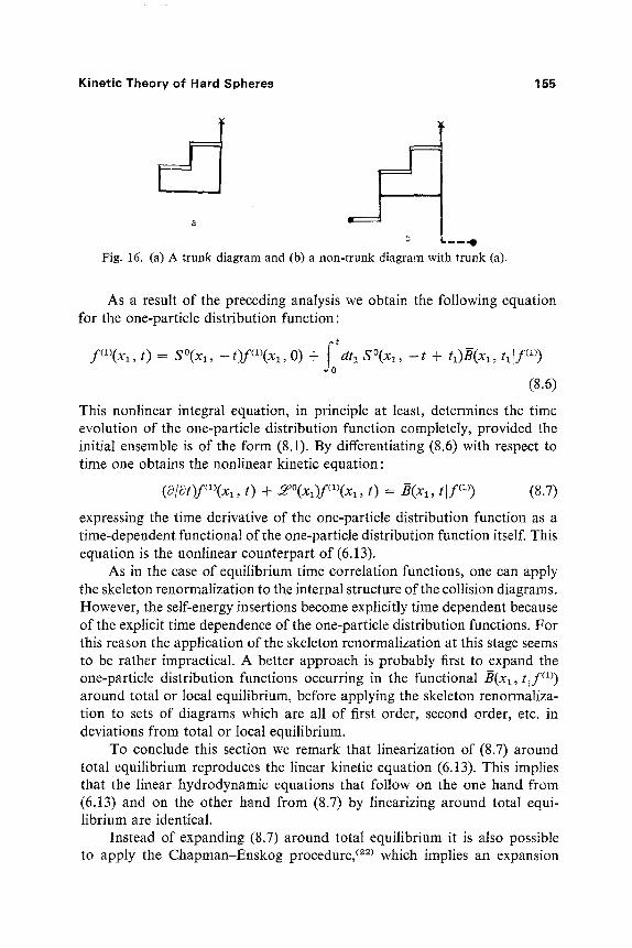
articulation point, respectively. But here the trivial case of a cut-point on the line segment running down from the top-cross is excluded. Trunk diagrams are defined again as diagrams without articulation points. As in Section 6, we distinguish between diagrams without or with dynamical bonds. The simplest diagram without dynamical bonds is the diagram consisting of the top-cross only. All other diagrams without dynamical bonds consist of a free propagator running down from the top-cross and a statistical vertex at the bottom (an example is given in Fig. 15). The sum of these diagrams represents the function S~ 0), as follows from the Mayer expansion of f(l~(xl, 0). All trunk diagrams with dynamical bonds consist of a barred regular collision diagram which is connected to the top-cross by one vertical line segment (an example is shown in Fig. 16a). The set/~ of all barred regular collision diagrams is larger here than it was in Section 8 : It contains diagrams with T-bonds from which no vertical lines run down, because DR 5a does not hold.
As in Section 5, all non-trunk diagrams with dynamical bonds can be constructed from trunk diagrams by attaching arbitrary diagrams from the expansion off(~(x~, t) at the lower cutoff levels of the vertical lines (see Fig. 16b). Hence the set of all diagrams with the same trunk represents the contribution of the latter, acting on a product of one-particle distribution functions which are attached at the lower cutoff levels of all the vertical lines, and evaluated at the corresponding times. For instance, the contribution of the diagram in Fig. 16a after the reduction to trunk diagrams is
f d x l ~ ( x - x l ) . dt lS~ - q ) dx2fz2 d t2S~ + q) J J o 1
f // x . dxa T23f(l~(x2, t2) dta S~ xa, - ta + t2)Tlaf(l~(xl, t3)f(~(xa, t3) J t2
The set of all collision diagrams is called the collision operator again. Here this operator produces a highly nonlinear functional of the function f of x and t on which it acts. This functional will be denoted as B(x, t[f). Again the contributions of instantaneous collision diagrams must be multiplied by a factor 3+(t).
Kinetic Theory of Hard Spheres 155
a
1
IZ - - - ' B
Fig. 16. (a) A trunk diagram and (b) a non-trunk diagram with trunk (a).
As a result of the preceding analysis we obtain the following equation for the one-particle distribution function:
fo' f(~)(xl, t) -= S~ -t)f(1)(xl, O) + dtl S~ - t + h)B(xl, h l f m)
(8.6)
This nonlinear integral equation, in principle at least, determines the time evolution of the one-particle distribution function completely, provided the initial ensemble is of the form (8.l). By differentiating (8.6) with respect to time one obtains the nonlinear kinetic equation:
(a/at)f(1)(xl, t) + 5r176 t) = B(xl, t l f (1)) (8.7)
expressing the time derivative of the one-particle distribution function as a time-dependent functional of the one-particle distribution function itself. This equation is the nonlinear counterpart of (6.13).
As in the case of equilibrium time correlation functions, one can apply the skeleton renormalization to the internal structure of the collision diagrams. However, the self-energy insertions become explicitly time dependent because of the explicit time dependence of the one-particle distribution functions. For this reason the application of the skeleton renormalization at this stage seems to be rather impractical. A better approach is probably first to expand the one-particle distribution functions occurring in the functional B(xl, t l f (~) around total or local equilibrium, before applying the skeleton renormaliza- tion to sets of diagrams which are all of first order, second order, etc. in deviations from total or local equilibrium.
To conclude this section we remark that linearization of (8.7) around total equilibrium reproduces the linear kinetic equation (6.13). This implies that the linear hydrodynamic equations that follow on the one hand from (6.13) and on the other hand from (8.7) by linearizing around total equi- librium are identical.
Instead of expanding (8.7) around total equilibrium it is also possible to apply the Chapman-Enskog procedure, (22~ which implies an expansion

156 H. van Beijeren and M. H. Ernst
about local equilibrium. This is a much more complicated procedure to follow here than it is in the case of the Boltzmann equation, because of the nonlocal and noninstantaneous character of the collision operator B. How- ever the results one would obtain would be very interesting, since the approach of a system to equilibrium is believed to proceed through a sequence of states close to local equilibrium but not necessarily close to total equilibrium.
9. D I S C U S S I O N
In the previous sections we have derived a linear kinetic equation for the one-partMe-one-particle correlation function and a nonlinear kinetic equa- tion for the one-particle distribution function by means of a diagrammatic expansion for these functions. Statistical correlations were expressed in Mayer functions and the streaming operator was represented by the binary collision expansion. A number of subsequent reduction steps led to the required kinetic equations, which turned out to be nonlocal and noninstantaneous. Diver- gences in the density expansions of the collision operators were removed by applying the skeleton renormalization. Now we want to make a comparison with the results of other investigators and mention the main applications of our theory.
Kinetic equations have been obtained with several methods. We list some of the most important ones below:
(i) The method of Bogoliubov, (1~ which is based on the functional assumption, implying that under certain initial conditions all the n-particle distribution functions become time-independent functionals of the one- particle distribution function after a short initial stage. Choh and Uhlenbeck have developed this theory further (2~ to obtain the first density correction to the Boltzmann equation and to the transport coefficients.
(ii) The cluster expansion method, developed by Green and Cohen. (3~ In this method the functional assumption is avoided. Relations between the n-particle distribution functions and the one-particle distribution function are constructed by means of cluster expansions, analogous to the methods used in the Mayer theory, and an attempt is made to prove the functional assumption of Bogoliubov's theory.
(iii) The diagrammatic methods developed by van Hove and co- workers (23~ and by the Brussels school. (4~
(iv) The binary collision expansion method, introduced by Zwanzig (1~ and used by several other authors. (8,~v,2~,2~ In this method the collision operator is expanded as a power series in the density. The individual terms in this expansion are obtained by inverting the density expansion of the exact propagator. Statistical correlations are always taken into account at the initial time.

Kinetic Theory of Hard Spheres 157
(v) Methods based on short-time expansions. (26'27~ These methods are well-suited to obtain exact kinetic equations for times much shorter than the mean free time, but generalizations valid for all times are not easy to obtain.
(vi) Weak coupling methods in which the collision operator is expanded in powers of the coupling strength. (28'29~
(vii) Projection operator methods. These were introduced by Zwanzig (3~ and were extended by Mori (al~ and used by several other investigators. Kinetic equations of the form (6.7) follow easily in these methods, but the collision operator is usually expressed as a complicated correlation function which cannot be calculated directly. In actual calculations projection operator tech- niques must therefore always be combined with some approximation scheme for the collision operator, such as a density expansion, (a2~ a weak coupling expansion, (28~ or a short-time expansion. (27~
(viii) The "fully renormalized kinetic theory" of Mazenko. (aa~ In this method the structure of the collision operator is analyzed extensively by algebraic methods before physical approximations are introduced.
In principle all these methods are equivalent. There are several papers in which the equivalence between certain methods is shown, for instance, between (ii) and (iii), (5~ and between (ii) and (iv). (3~ In practical applica- tions, however, it mostly turns out that, dependent on the problem one considers, certain methods are preferable.
The method developed in this paper is based on (iv); however, the analysis has been carried much further. The main improvement is that the statistical correlations are taken into account in the internal structure of the collision operators. The whole analysis is based on the application of the shifting procedure, which follows from a commutation relation between Mayer functions and free streaming operators. As a consequence the structure of the collision operators is much simpler in our representation than in Zwanzig's original version.
What are the advantages of our formulation of the kinetic equations ? First, the collision operator is expanded as an infinite series of diagrams,
each representing a well-defined dynamical event. In nondJagrammatic methods, such as (i) and (ii), n-body collision operators are expressed in terms of the formal solution of the isolated n-body problems. Before performing explicit calculations these expressions must be analyzed further in terms of different collision sequences. In the diagrammatic representations this analysis is automatically carried out. The diagrammatic method used here has the additional advantage that statistical correlations are taken into account at the most relevant times. This again simplifies actual calculations considerably.
Second, we expect that the divergences in the density expansion of the transport coefficients are removed in a systematic way by the application of the skeleton renormalization, provided the transport coefficients exist at all

158 H. van Beijeren and M. H. Ernst
for the model under consideration. Of course these renormalized expansions are still completely formal, since no estimates of the magnitude of the indi- vidual terms have been given, nor have any upper or lower bounds been established for these terms. Similar renormalization procedures have been applied in (vii).
Third, in many formulations of the kinetic equations it is not simple to take initial statistical correlations into account [e.g., in (i)-(iv)]. In our formulation these col"relations are systematically taken care of. As a result the obtained kinetic equations are not restricted to low densities, nor are there any restrictions that the time should be either long or short.
Finally, our approach has the advantage that it reproduces several different nonequilibrium results for the hard-sphere system from a unified point of view. We mention the main results below and refer to Ref. 13 for details.
The Boltzmann equation is obtained by keeping only the leading term in the density expansion of the collision operator. This means that in Eq. (7.1) for the function F(x, x', t) only the first two terms on the right-hand side survive, giving rise to a linearized Boltzmann equation. In the nonlinear equation (8.7) the collision operator reduces to
BB(xl, t l f (1~) = f dx2 T12f~l)(xl, t)f(1)(x2, t) (9.1)
This form of the nonlinear binary collision term has also been derived by Bogoliubov. (1) The collision operator T12 is slightly nonlocal and therefore different from the usual Boltzmann operator, but for low densities the nonlocality may be neglected in most cases.
The Enskog equation is obtained by keeping only the instantaneous diagrams in the expansion of the collision operator. These are all diagrams which contain no vertical line segments and are therefore proportional to a 8-function $+(t). In the nonlinear case this leads to a new kinetic equation of the form (8.7) with a modified Enskog collision operator (35)
BM~(x~, t l f (1~) = f dx2 T~2x(rl, r2)f(1)(xl, t)f(1)(x2, t) (9.2)
The nonuniform pair distribution function g(r~, r2) = (1 + f~2)x(r~, r2) is defined in terms of a nonuniform equilibrium ensemble pnu(P, t) of the form (2.4), where the external potential V(r) has been chosen such that pn~ produces the correct density n(r, t) everywhere (note that for the determination of x the choice of the temperature is irrelevant). The explicit form of g(r~, r2) in terms of Pnu is
r2) = f dP Onu(P) ~ ~ 3(r~ - r,) 8(r2 - rj) (9.3) n(rl)n(r2)g(rz ,

Kinetic Theory of Hard Spheres 159
This can be expressed as a nonlocal functional of the density n(r) (see StelF19~), in the form of a Mayer expansion/19'35) The modified Enskog collision operator differs from the usual nonlinear Enskog collision operator
BE(x1, t l f ~1~) = f dx2 Tmxo(r12[n(�89 + �89 t)f(l~(x2, t) (9.4)
Here the x function is related to the equilibrium pair distribution function go(r~2) = (1 +f~2)xo(r~2tn) with the (uniform) density taken to be n(�89 + �89 However, in a one-component system the usual Enskog equation and the modified Enskog equation give rise to the same Navier-Stokes equa- tions and related transport coefficients. Our equation is straightforwardly generalized to the case of hard-sphere mixtures. Then it leads to Navier- Stokes equations which are different from those obtained by previous exten- sions of the Enskog equation. It is interesting to observe that for mixtures the predictions based on the modified Enskog equation are consistent with the laws of irreversible thermodynamics, especially with the Onsager relations, whereas this is not the case in the existing extensions of Enskog's theory for mixtures. This has been discussed in detail in Ref. 35. Recently Kincaid has investigated the numerical differences between the predictions of the modified Enskog theory and those of previous theories/36~ For the binary diffusion coefficient he found differences up to about 30~o. An H-theorem for the modified Enskog equation has been proved by R6sibois. (37~
In the linear theory the instantaneous diagrams, examples of which are given in Figs. l la-d, lead to a modified linear Enskog equation [compare (6.7)] of form
[~3/~3t - ~~ - ~ME(X~)]h(x~, t) = 0 (9.5a) with
t ~ ( BME(Xl) = J dx2 ~o(x2)T12~[1 + G(rz, r2)](1 + PXxX2)
Here ~0(x~) = ncpo(V 0 is defined in (2.10); G(rl, r2) is the equilibrium pair correlation function (6.3); and H(rl, r2]r3) represents the set of all Mayer graphs that can be obtained by replacing one field point by a root-point in the Mayer graphs representing the pair correlation function G(r~, r2) (see Ref. 19). Furthermore, h(x, t) represents either the equilibrium one-particle time correlation function F(x, x'; t) or the nonequilibrium distribution function, i.e.,f~l)(x, t) = ~v(x){1 + h(x, t)}. In case no external forces are present (9.5) can be put into a more convenient form, (35~ which reads for the Fourier transform of h(x, t), defined in (6.9a),
{~/~t + ik.v - xAk(v)}hk(v, t) = ik-v[Ck - xf~] 3nk (9.6)

160 H. van Beijeren and M. H. Ernst
Here Ck, as in (6.12), is the Fourier transform of the direct correlation function;f~ is the Fourier transform of the Mayer f-function, given in (2.7); and x = xo(r~2 = e[n) is the equilibrium pair distribution function at contact. Finally,
~nk(t) = n f dv %(v)h~(v, t) (9.7a)
Ak(vl)h(h) = n=2f dr2 f d~ (v12"b)#(vx2"~) (9.7b)
x {h(v~*) - h(vl) + [exp(-ik.~r)]h(v2*) - [exp(ik.~r)lh(v2)}
The linear modified Enskog equation (9.5) or (9.6) follows also by linearizing (9.2), as was shown in Ref. 35. Percus et al., ~26~ Konijnendijk and van Leeuwen, C2v and Mazenko ~a3~ have obtained this equation as the limit of the complete kinetic equation as time goes to zero. In order to emphasize the differences between (9.5b) and the usual Enskog equation we consider the linearized form of (9.4). Inserting this into the linearized kinetic equation for the distribution function, one recovers (9.6) with the right-hand side replaced by
�89 vn(dxidn)fkt2 8nk (9.8)
In the case of tagged particles where h~(x, t) represents F~(x, x'; t) or the distribution function fm~(x, t) = q~(x)[1 + h~(x, t)] of the tagged particle, the instantaneous diagrams yield the usual linear Enskog equation, i.e.,
[O/~t - s - BS~(x)lh~(x, t) = 0 (9.9a)
with / ,
B~E(Xl) = X J dx2 ~o(x2)TI2 (9.9b)
From the linear kinetic equation (6.13) for F(x, x'; t) one can derive linearized hydrodynamic equations. The transport coefficients are expressed as matrix elements of the collision operator and its inverse. They can be identified immediately with the Green-Kubo formulas, expressing transport coefficients as time integrals over equilibrium time correlation functions. From the nonlinear kinetic equation nonlinear hydrodynamic equations can be derived in principle by generalizing the Chapman-Enskog method of solution. However, this method leads to serious complications because of the nonlocal and noninstantaneous character of the complete collision operator. In a study on nonlinear viscous flow such a nonlinear kinetic equation was used in Ref. 38. The collision term there is, apart from the nonlinear Boltz- mann term, precisely the nonlinear r!ng term (e.g., the diagrams of Figs. 1 If and 1 lg without a bottom-cross) and all nonlinear repeated ring terms (an

Kinetic Theory of Hard Spheres 161
example is given in Fig. 1 lc, again dropping the bottom-cross). The only difference is that we distinguish here between T and T operators, which is not done in Ref. 38. This difference has no effect on the results obtained there to dominant order in the density.
Another interesting application is the study of the density expansion of the transport coefficients. In three dimensions the triple collision term, i.e., the first te'rm beyond the Boltzmann collision term, is convergent. It was discussed first by Choh and Uhlenbeck. (2) In our kinetic equations the form of this term for the hard-sphere case follows automatically from the expan- sion of the collision operator by collecting all three-particle collision diagrams (e.g., Figs. 1 lc-h). In the linearized theory it reads
~3(xl, t) = f dx~ dx3 ~(x~)~(x~)
• 3+(t) T12f~f23(1 + Px~2 + Pxzm)
P~I~)
x s~%rl~(1 + P~lx~)
f - ~ x S~ + Px~m)
f - o f x S%T~(1 + P ~ ) (9.10)
where S% is a short-hand notation for S~ x2, t). To obtain (9.10) we have used theorems by Sandri et al., Murphy and Cohen, and Hoegy and Sengers, (89) restricting the number of collisions (real or virtual) between three isolated, identical, smooth hard spheres to four, in a few well-defined sequences. For a review of numerical calculations on the triple-collision contributions to the transport coefficients in three dimensions, see Ref. 40.
Beyond the order n 2 in three dimensions and the order n in two dimen- sions the individual terms in the density expansion of the collision operator give divergent contributions to the transport coefficients. For that reason we had to introduce the skeleton renormalization. The contributions of the renormalized diagrams are well-behaved (at least in three dimensions), but depend on the density in a nonanalytic way. The leading nonanalyticities stem from the so-called ring term, represented by the diagram in Fig. 14f. The

162 H. van Beijeren and M. H. Ernst
density dependence of this term has been studied by Kawasaki and Oppen- heim.(8~, 18 Their analysis can be reproduced easily from our kinetic equations.
The long-time behavior of equilibrium time correlation functions can also be calculated with the aid of kinetic theory. For low densities this has been done by Dorfman and Cohen. (11) For the time correlation functions occurring in the Green-Kubo formulas, such as the velocity autocorrelation function, they find a long-time behavior proportional to t-~/2 in d dimensions. They also obtained an extension to higher densities for hard-sphere systems (4t) by supplying the Enskog collision operator (9.5b) with a consistent approxi- mation for the ring term. For densities not too close to the freezing density this theory is in excellent agreement with molecular dynamics data.
From our kinetic equations the long-time behavior of equilibrium time correlation functions can be obtained for general fluid densities, and also the so-called kinetic-potential and potential-potential contributions to these correlation functions can be treated. In three dimensions the results agree completely with the results from mode-mode coupling theoryJ TM Further- more, the latter can be justified to some extent by estimating the terms that are neglected in mode-mode coupling theory. (42~ In two dimensions the t - ~ behavior is modified for very long times and changes finally to a behavior as [t(log t)1/2] -1. It is easy to extend the theory so as to calculate four-point correlation functions like the ones occurring in formal correlation function expressions for the super Burnett coefficients. (42~ These are found to behave for long times as t 1/2 in three dimensions and as t (for times which are not extremely long) in two dimensions. C~2~
Finally we mention that the linear theory can be extended easily to m- particle-n-particle equilibrium time correlation functions, as is carried out in the Appendix, while the nonlinear theory can be used to express the n-particle distribution functions as time-dependent functionals of the one-particle distribution function.
We conclude by giving some other possible applications and extensions of the theory presented here.
(i) It would be very useful if, under certain conditions, one could find convergence proofs for the individual renormalized diagrams contributing to the collision operator as well as for the whole series. To date only a few results have been obtained in this direction. Lanford ( ~ has shown rigorously that the nonlinear kinetic equation for the one-particle distribution function reduces to the Boltzmann equation in the limit of vanishing particle density (the Boltzmann-Grad limit) for a time interval which is a finite fraction of the mean free time. For this he has to require that the initial spatial correlations do not extend beyond a range proportional to the hard-sphere diameter. For
18 Numerical estimates of the resulting contributions to the transport coefficients have been made by Pomeau e t al . ~8~ and by Kan and Dorfman. ~49~

Kinetic Theory of Hard Spheres 163
the equilibrium velocity autocorrelation function a stronger result has been obtained~44~: in the Boltzmann-Grad limit this function satisfies the Lorentz- Boltzmann equation for all times. The limit is not uniform for all times, however; this means, for instance, that one cannot prove that the coefficient of self-diffusion approaches its Lorentz-Boltzmann value. For the Lorentz gas it is straightforward to show by Lanford's methods that the velocity autocorrelation function satisfies the Lorentz-Boltzmann equation in the Boltzmann-Grad limit. ~45~ Spohn and Lebowitz have discussed the problems of steady heat flow for this system. (46~
(ii) The derivation of nonlinear hydrodynamic equations from the non- linear kinetic equation (8.7) by making an expansion around local equilibrium. This procedure is more difficult here than it is in the case of the Boltzmann or Enskog equation. The reason is that the collision operator contains many contributions exhibiting a slow time decay, such as that of the ring diagram.
An interesting question is the following: Can equilibrium time correla- tion functions be described in some sense by nonlinear equations, and especially can their long-time behavior be obtained from such equations ~v~ ?
(iii) The derivation of nonlinear kinetic equations for initial ensembles which allow for more general correlations between the positions and velocities of the particles than those contained in (8.1).
(iv) A further investigation of the density dependence of transport coefficients. In principle it seems possible with our theory to make a classi- fication of diagrams which contribute to a given order in the density n, where we allow for nonanalytic functions, containing, for instance, noninteger powers of n or powers of log n. However, the actual calculation of all these terms is very difficult; it is already so for the first nonanalytic term in three dimensions.
(v) The study of Brownian motion by applying the kinetic equation for the one-particle self-correlation function to a Brownian particle. This has been undertaken by one of the authors (HvB) in collaboration with Dorfman.
(vi) The extension to more general potentials of finite range. Very little is known about the derivation of kinetic equations in the presence of short- range attractive forces between the particles. The main complication is the possibility of bound states between two or more particles. If one extends the hard-sphere interaction by an attractive square well, the interactions between the particles remain instantaneous. Therefore it seems plausible that our techniques can be applied to this model with only a few changes. The resulting kinetic equations would be interesting, especially at moderate and high densities. Furthermore, the theory described here can be extended to more general potentials of finite range. Then the binary collision expansion must be generalized to a multiple collision expansion, taking into account inter- actions among more than two particles and of finite duration. This makes the theory much more complicated.

164 H. van Beijeren and M. H. Ernst
It would be interesting to know whether also in the case where a small attractive piece is present some kind of Enskog equation could be obtained by considering a short-time limit.
A P P E N D I X . m - P A R T I C L E - n - P A R T I C L E C O R R E L A T I O N F U N C T I O N S
Our method can be extended directly to m-particle-n-particle equilibrium time correlation functions, defined as
r([m]; [n]; t ) =- F(xl , . . . , Xm; Xl',..., X,' ; t )
= ( y. ~ ~(x~- x,~(0)) t l . . . i ra ~ = 1
x ~( ~ 1-~ 3 (x l ' - x h ( t ) ) - n(xt', .... x n ' ) ~ (A1) \ J l . . d n ! = 1 2 / e q
The summations are subject to the restrictions i~ r iz and j~ r j, if k r l. The function n(xl .... , x.) is the equilibrium n-particle distribution function
n(x, .... , x , ) = ~ ~ 1-~ ~(x~- x,~))q (A2) t l . . , i n k = l
After introducing (2.11b) into (A1) one can make a diagrammatic representation of this expression along the lines sketched in Section 3. All the g-functions 3(xk - xik(0)) are represented by a cross at the top and the 8- functions 3(x/ - xjt ) by a cross at the bottom. Hence (A1) can be expressed as
F([m]; [n]; t) = {/30([m], [n]) - Do([ml)n([n])}/Z~r (A3)
where/90([m], [hi) and/7o([m]) are the sets of all diagrams with m top-crosses and n [resp. zero] bottom-crosses satisfying DRs 1-3. The DRs 4 and 5 can be introduced as before, after which the sets Do([m], [n]) and /9o([m]) in (A3) can be replaced by the corresponding sets Ol([m], [n]) and B~([m]). Also, the reduction to linked diagrams goes as before, with the following important convention: all the top-crosses are considered to be linked among themselves by virtual bonds and so are all bottom-crosses but no such virtual bonds are made between top-crosses and bottom-crosses. After the reduction to linked diagrams the following expression is obtained for the correlation functions:
F([m]; [n]; t) = Co(Ira], [hi) (A4)
where Co([m], In]) is the subset of all linked diagrams belonging to/91([m], In]). The shifting procedure goes as in Section 4, with the following proviso: when decomposing a diagram into star factors and applying the cutoff rules to the latter, one has to respect the virtual bonds between top-crosses and between
Kinetic Theory of Hard Spheres 165
bottom-crosses. This implies that there is always a star factor containing all the top-crosses and a star factor (which may be the same one) containing all the bottom-crosses. Also, the reduction to trunk diagrams goes as before, but again one has to respect the virtual bonds while looking for articulation points. The correlation functions may then be expressed as
F([m]; [n]; t) = C2([m], [n]) (A5)
where C2 is the set of all barred regular trunk diagrams, satisfying DRs 1"- 12". However, D R I* has to be generalized slightly so as to allow for diagrams with arbitrary numbers of top and bot tom crosses.
For the one-particle-two-particle, two-particle-one-particle, and two- particle-two-particle correlation functions one can obtain Dyson-like equations again, but these are more complicated than for the one-particle- one-particle correlation function. For details we refer to Ref. 13.
The skeleton renormalization finally can be applied to the sets C2([m], [hi) representing the F([m]; [n]; t), irrespective of the values of m and n.
A more extended treatment of the formalism for the m-particle-n-particle correlation functions, as well as for the m-particle distribution functions in the nonequilibrium case, can be found in Ref. 13.
A C K N O W L E D G M E N T S
The authors want to thank J. R. Dorfman for some useful remarks about the manuscript. The research reported in this paper was clone for a doctoral thesis at the Katholieke Universiteit Nijmegen. We acknowledge the courtesy of this university in making the original figures from the thesis available for this paper.
REFERENCES
1. N. N. Bogoliubov, J. Phys. USSR 10:257 (1946); English translation in Studies in Statistical Mechanics, Vol. I, J. de Boer and G. E. Uhlenbeck, eds. (North-Holland, Amsterdam, 1962).
2. S. T. Choh, The kinetic theory of phenomena in dense gases, Diss., Univ. of Michigan (1958).
3. M. S. Green and R. A. Piccirelli, Phys. Rev. 132:1388 (1963); E. G. D. Cohen, in Fundamental Problems in Statistical Mechanics (North-Holland, Amsterdam, 1962).
4. I. Prigogine, Non-Equilibrium Statistical Mechanics (Interscience, New York, 1962). 5. J. Brocas, Advan. Chem. Phys. 11:317 (1967). 6. M. S. Green, J. Chem. Phys. 20:1281 (1952); 22:398 (1954); R. Kubo and K.
Tomita, J. Phys. Soc. Japan 9:888 (1954); R. Kubo, in Lectures in Theoretical Physics (Interscience, New York, 1959), Vol. I, p. 120.
7. J. Weinstock, Phys. Rev. 132:454 (1963); 140:A460 (1965); J. R. Dorfman and E. G. D. Cohen, Phys. Lett. 16:124 (1965); E. A. Frieman and R. Goldman, Bull. Am. Phys. Soc. 10:531 (1965).
166 H, van Beijeren and M. H. Ernst
8. K. Kawasaki and I. Oppenheim, Phys. Rev. 139:A1763 (1965). 9. B. J. Alder and T. E. Wainwright, Phys. Rev. Lett. 18:988 (1967); Phys. Rev. A
1:18 (1970). 10. M. H. Ernst, E. H. Hauge, and J. M. J. van Leeuwen, Phys. Rev. Lett. 25:1254
(1970); Phys. Lett. 34A:419 (1971); Phys. Rev. A 4:2055 (1971). 11. J. R. Dorfman and E. G. D. Cohen, Phys. Rev. Lett. 25:1257 (1970); Phys. Rev. A
6:776 (1972). 12. C. Bruin, Physica 72:261 (1974); Doctoral thesis (Delft University Press, 1978). 13. H. van Beijeren, Diss., Katholieke Universiteit Nijmegen. 14. R. Zwanzig, Phys. Rev. 129:486 (1963). 15. M. H. Ernst, J. R. Dorfman, W. Hoegy, and J. M. J. van Leeuwen, Physica 45:127
(1969). 16. J. V. Sengers, M. H. Ernst, and D. T. Gillespie, J. Chem. Phys. 56:5583 (1972). 17. J. M. J. van Leeuwen and S. Yip, Phys. Rev. 139:Al183 (1965). 18. C. Bloch, in Studies in Statistical Mechanics, Vol. III, J. de Boer and G. E. Uhlen-
beck, eds. (North-Holland, Amsterdam, 1965), p. 35; J. W. Essam and M. E. Fisher, Rev. Mod. Phys. 42:272 (1970).
19. G. E. Uhlenbeck and G. W. Ford, in Studies in Statistical Mechanics, Vol. I, J. de Boer and G. E. Uhlenbeck, eds. (North-Holland, Amsterdam, 1962); G. Stelt, in The Equilibrium Theory of Classical Fluids, H. L. Frisch and J. L. Lebowitz, eds. (Benjamin, New York, 1964).
20. L. S. Ornstein and F. Zernike, Proc. Kon. Ned. Akad. Wetensch. 17:793 (1914). 21. M. H. Ernst, L. K. Haines, and J. R. Dorfman, Rev. Mod. Phys. 41:296 (1969). 22. S. Chapman and T. G. Cowling, The Mathematical Theory of Nonuniform Gases
(University Press, Cambridge, 1960). 23. L. van Hove, in Fundamental Problems in Statistical Mechanics, E. G. D. Cohen,
ed. (North-Holland, Amsterdam, 1962). 24, J. M. J. van Leeuwen and A. Weyland, Physica 36:457 (1967); 38:35 (1968). 25. E. H. Hauge and E. G. D. Cohen, Y. Math. Phys. 10:397 (1969). 26. J. L. Lebowitz and J. K. Percus, Phys. Rev. 155:122 (1967); J. L. Lebowitz, J. K.
Percus, and J. Sykes, Phys. Rev. 171 : 224 (1968) ; J. Sykes, J. Stat. Phys. 8: 279 (1973). 27. H. H. U. Konijnendijk and J. M. J. van Leeuwen, Physica 64:342 (1973). 28. A. Z. Akcasu and J. J. Duderstadt, Phys. Rev. 188:479 (1969). 29. D. Forster and P. C. Martin, Phys. Rev. A 2:1575 (1970). 30. R. Zwanzig, in Lectures in Theoretical Physics, Vol. III (Interscience, New York,
1961). 31. H. Mori, Progr. Theor. Phys. 33:423 (1965). 32. M. H. Ernst, in Lectures in Theoretical Physics, Vol. IXC (Gordon and Breach, New
York, 1967). 33. G. F. Mazenko, Phys. Rev. A 7:209, 222 (1973); 9:360 (1974). 34. L. K. Haines, Diss. ; Technical note BN-460, Univ. of Maryland (1966). 35. H. van Beijeren and M. H. Ernst, Physica 68:437 (1973); 70:25 (1973). 36. J. M. Kincaid, Phys. Left. 64A:429 (1978). 37. P. R6sibois, J. Stat. Phys. 19:593 (1978) Physica 94A:1 (1974). 38. M. H. Ernst, B. Cichocki, J. R. Dorfman, J. Sharma, and H. van Beijeren, J. Stat.
Phys. 18:237 (1978). 39. G. Sandri, R. D. Sullivan, and P. Norem, Phys. Rev. Lett. 13:743 (1964); E. G. D.
Cohen, in Lectures in Theoretical Physics, Vol. VIIIA (Univ. of Colorado, Boulder, 1966); T. J. Murphy, unpublished; W. R. Hoegy and J. V. Sengers, Phys. Rev. A 2:2461 (1970).

Kinetic Theory of Hard Spheres 167
40. J. V. Sengers, D. T. Gillespie, and J. J. Perez-Esandi, Physica 90A:365 (1978). 41. J. R. Dorfman and E. G. D. Cohen, Phys. Rev. A 12:292 (1975). 42. I. M. de Schepper, H. van Beijeren, and M. H. Ernst, Physica 75:1 (1974); I. M. de
Schepper and M. H. Ernst, Physica 87A:35 (1977); Physica 93A:61 t (1978). 43. O. E. Lanford, in Dynamical Systems, J. Moser, ed. (Springer, New York, 1975). 44. H. van Beijeren, J. L. Lebowitz, O. E. Lanford, and H. Spohn, to be published. 45. H. Spohn, Comm. Math. Phys. 60:277 (1978). 46. J. L. Lebowitz and H. Spohn, J. Stat. Phys. 19:633 (1978). 47. R. Zwanzig, K. S. J. Nordholm, and W. C. Mitchell, Phys. Rev. A 5:2680 (1972). 48. Y. Pomeau and A. Gervois, Phys. Rev. A 9:2196 (1974); A. Gervois, C. Normand
Alle, and Y. Pomeau, Phys. Rev. A 12:1570 (1975). 49. Y. Kan and J. R. Dorfman, Phys. Rev. A 16:2447 (1977).