kinetics and modeling of the radical polymerization of

Kinetics and Modeling of the Radical

Polymerization of Acrylic Acid and of

Methacrylic Acid in Aqueous Solution

Dissertation

zur Erlangung des mathematisch-naturwissenschaftlichen Doktorgrades

„Doctor rerum naturalium“

der Georg-August-Universität Göttingen

im Promotionsprogramm Chemie

der Georg-August University School of Science (GAUSS)

vorgelegt von

Nils Friedrich Gunter Wittenberg

aus Hamburg

Göttingen, 2013

Betreuungsausschuss

Prof. Dr. M. Buback, Technische und Makromolekulare Chemie, Institut für Physikalische

Chemie, Georg-August-Universität Göttingen

Prof. Dr. P. Vana, MBA, Makromolekulare Chemie, Institut für Physikalische Chemie,

Georg-August-Universität Göttingen

Mitglieder der Prüfungskommission

Referent: Prof. Dr. M. Buback, Technische und Makromolekulare Chemie, Institut für

Physikalische Chemie, Georg-August-Universität Göttingen

Korreferent: Prof. Dr. P. Vana, MBA, Makromolekulare Chemie, Institut für Physikalische


Weitere Mitglieder der Prüfungskommission:

Prof. Dr. G. Echold, Physikalische Chemie fester Körper, Institut für Physikalische Chemie,


Prof. Dr. B. Geil, Biophysikalische Chemie, Institut für Physikalische Chemie, Georg-August-

Universität Göttingen

Jun.-Prof. Dr. R. Mata, Computerchemie und Biochemie,Institut für Physikalische Chemie,


Prof. Dr. A. Wodtke, Physikalische Chemie I / Humboldt-Professur, Institut für Physikalische


Tag der mündlichen Prüfung: 24.10.2013

Meiner Familie

Table of Contents

V

Table of Contents

Abstract .......................................................................................................................... 1

1 Introduction ............................................................................................................ 3

2 Theoretical Background ......................................................................................... 7

2.1 General Aspects of Radical Stability and Reactivity ...................................... 7

2.2 Ideal Polymerization Kinetics of Radical Polymerization .............................. 9

2.2.1 Formation of Radicals and Initiation ..................................................... 10

2.2.2 Propagation ............................................................................................. 13

2.2.3 Termination ............................................................................................ 13

2.2.4 Steady State Kinetics ............................................................................. 14

2.3 Additional Reactions...................................................................................... 15

2.3.1 Transfer Reactions to Small Molecules .................................................. 15

2.3.2 Intermolecular Transfer to Polymer ...................................................... 19

2.3.3 Intramolecular Transfer to Polymer – Backbiting ................................ 20

2.3.1 β-Scission Reaction ................................................................................. 24

2.3.2 Retardation and Inhibition .................................................................... 26

2.4 Influences on Rate Coefficients ..................................................................... 27

2.4.1 Temperature and Pressure ..................................................................... 29

2.4.2 Concentration ......................................................................................... 30

2.4.3 Ionization ................................................................................................ 33

2.4.4 Chain Length .......................................................................................... 38

2.4.5 Conversion .............................................................................................. 45

2.5 Computer Modeling of Polymerizations ........................................................ 51

3 Materials, Experimental Procedures and Data Evaluation ................................ 55

3.1 Chemicals ....................................................................................................... 55

Table of Contents

VI

3.1.1 Monomers ............................................................................................... 55

3.1.2 Solvents .................................................................................................. 57

3.1.3 Initiators ................................................................................................. 58

3.1.4 Inhibitors ................................................................................................ 60

3.1.5 Substances used to prepare Buffer Solutions ........................................ 60

3.1.6 Others ..................................................................................................... 61

3.2 Purification Procedures ................................................................................. 63

3.3 NIR ................................................................................................................ 63

3.3.1 Setup ....................................................................................................... 63

3.3.2 Thermally initiated Polymerization in a Cuvette.................................. 64

3.3.3 Photoinitiated Polymerization in a Cuvette .......................................... 65

3.3.4 Degree of Monomer Conversion ............................................................. 65

3.4 EPR ................................................................................................................ 69

3.4.1 Setup ....................................................................................................... 69

3.4.2 Organic Samples .................................................................................... 69

3.4.3 Aqueous Samples ................................................................................... 70

3.4.1 Deconvolution of Spectra ........................................................................ 70

3.4.2 Calibration .............................................................................................. 70

3.5 NMR ............................................................................................................... 71

3.5.1 Quantitative 1H-NMR ............................................................................ 71

3.5.2 Quantitative 13C-NMR ........................................................................... 72

3.5.3 Polymerization in NMR Sample Tube ................................................... 77

3.6 Density Measurement ................................................................................... 78

3.7 Viscosity Measurement ................................................................................. 78

3.7.1 Important Features of Polymer Solutions ............................................. 79

3.7.2 Polymerization in Viscosity Measurement Capillary ............................ 80

3.8 Preparation of Buffer Solutions .................................................................... 80

3.9 SEC ................................................................................................................ 81

Table of Contents

VII

3.10 ESI-MS ........................................................................................................... 81

3.11 HPLC ............................................................................................................. 81

3.12 pH-Meter ........................................................................................................ 82

3.13 High-Temperature Polymerizations.............................................................. 83

3.13.1 Stopped-Flow experiments in High-Pressure Cell ................................. 84

3.13.2 Polymerization in a Tubular Reactor ..................................................... 84

3.14 Other Setups for Polymerization ................................................................... 88

3.14.1 1 L Automated Reactor ........................................................................... 88

3.14.2 Polymerization in a Heating Block ........................................................ 89

3.14.3 Polymerization in a Flask ...................................................................... 89

3.14.4 Polymerization in a Lined Flask ............................................................ 90

3.15 Computer Programs ...................................................................................... 90

3.15.1 Curve Fitting .......................................................................................... 90

3.15.2 Determination of Joint Confidence Regions .......................................... 90

3.15.3 Simulation .............................................................................................. 91

3.16 Error Estimate ............................................................................................... 91

4 Methacrylic Acid ................................................................................................... 95

4.1 Chain-Transfer to 2-Mercaptoethanol .......................................................... 96

4.1.1 Chain Transfer Constants deduced by the Mayo Method ..................... 97

4.1.2 Chain Transfer Constants deduced by the CLD Method .................... 101

4.1.3 Comparison of Mayo and CLD methods .............................................. 103

4.2 Model development for Non-ionized Methacrylic Acid ............................... 106

4.2.1 Modeling Polymerization at Medium initial Monomer Content ......... 110

4.2.2 Modeling Polymerization at Low initial Monomer Content ................ 123

5 Acrylic Acid ......................................................................................................... 141

5.1 Model development for Non-ionized Acrylic Acid ....................................... 142

5.1.1 Initiator Kinetics .................................................................................. 146

5.1.2 Evaluation of kps data ........................................................................... 149

Table of Contents

VIII

5.1.3 Evaluation of kt and Viscosity data ..................................................... 155

5.1.4 Determination kbb by 13C-NMR ............................................................ 159

5.1.5 BA as a Model for AA to estimate CCTAt by EPR .................................. 164

5.1.6 CCTAs of ME with AA ............................................................................. 175

5.1.7 Determination of kp for AA Macromonomers by 1H-NMR................... 178

5.1.8 Modeling Polymerization at 35 to 80 °C .............................................. 181

5.1.9 Modeling Polymerization at High Temperature .................................. 188

5.2 Model Development for Ionized Acrylic Acid .............................................. 197

5.2.1 kp of Fully Ionized AA and dependence on Ionic Strength .................. 198

5.2.2 kt at Full Ionization .............................................................................. 201

5.2.3 kbb at Full Ionization and dependence on Ionic Strength .................... 202

5.2.4 Density .................................................................................................. 204

5.2.5 Modeling the Polymerization of Fully Ionized AA ............................... 208

5.2.6 The dependence of kp on the Degree of Ionization ............................... 212

5.2.7 The dependence of kt on the Degree of Ionization ............................... 214

5.2.8 The dependence of kbb on the Degree of Ionization.............................. 217

5.2.9 β-Scission .............................................................................................. 219

5.2.10 The pKA of pAA ..................................................................................... 220

5.2.11 Modeling the Polymerization of Partly Ionized AA ............................. 224

6 Acrylamide .......................................................................................................... 231

7 Closing Remarks................................................................................................. 243

Appendix .................................................................................................................... 251

Abbreviations and Symbols ....................................................................................... 263

References .................................................................................................................. 271

Abstract

1

Abstract

The radical polymerization of methacrylic acid, acrylic acid and acrylamide in

aqueous solution has been investigated. Detailed kinetic models for both acrylic acid,

AA, and methacrylic acid, MAA, have been developed applying the program

PREDICITM. Good representation of experimental conversion vs. time profiles and

molar mass distributions as well as, in case of AA, the branching level could be

achieved.

The polymerization of MAA has been studied at 35 and 50 °C with focus on the

influence of 2-mercaptoethanol, ME, as chain transfer agent, CTA, on reaction

kinetics. The rate coefficient of transfer to CTA, tr,CTA ,k was measured for different

monomer levels by the Mayo and the chain length distribution procedure. The ratio

of tr,CTAk to the propagation rate coefficient, pk , is independent of monomer to water

ratio while both rate coefficients increase by approximately one order of magnitude

in passing from bulk to dilute aqueous solution.

It was found that addition of CTA reduces the rate of MAA polymerization by two

effects on t .k At negligible monomer conversion, tk increases towards higher

content of CTA, because average chain length is reduced by the CTA. Chain-length

dependent termination may be represented by adopting the composite model, which

is a well-established theory to describe chain-length dependency of termination of

macroradicals of identical size. The composite model could be applied to average

chain length. The reduction of tk towards higher degrees of monomer conversion

(Norrish–Trommsdorff or gel effect) becomes weaker towards higher levels of CTA,

which could be described by correlating the intensity of the gel effect to molar mass

of polymer in solution.

Abstract

2

The polymerization of non-ionized AA in aqueous solution has been studied between

35 and 80 °C with and without ME as CTA. Chain-length dependent termination

was taken into account for modeling as for MAA. During AA polymerization a 1,5-

hydrogen shift (backbiting) takes place transforming the secondary propagating

radical, SPR, into a tertiary midchain radical, MCR, the kinetics of which were

included into the model. The backbiting reaction was quantified via 13C-NMR, the

other MCR reactions were estimated from conversion vs. time profiles. By measuring

the MCR fraction during butyl acrylate, BA, polymerization via electron

paramagnetic resonance, EPR, it could be shown that the transfer of MCRs to CTA is

not an important reaction path. BA can be used as AA model compound so that the

same finding should also apply for AA polymerizations in aqueous phase. Chain

transfer of SPRs of AA was measured by the Mayo method.

The model was extended towards high-temperature polymerization of AA between 90

and 170 °C, where -scission and propagation of macromonomers need to be

considered. Moreover, a model for the polymerization of ionized AA was developed,

which takes numerous dependencies of rate coefficients on ionization and ionic

strength into account, e.g., propagation is reduced by ionization of monomer, but to a

higher extent for lower monomer concentration. Moreover, propagation of ionized

monomer augments towards higher ionic strength. MCRs were found during

acrylamide polymerization via EPR revealing the backbiting reaction to apply for

this monomer as well. Thus, the kinetic scheme is the same as for AA

polymerization.

Parts of this thesis have already been published:

Wittenberg, N. F. G.; Buback, M.; Stach, M.; Lacík, I. Macromol. Chem. Phys. 2012,

213, 2653–2658.

Wittenberg, N. F. G.; Buback, M.; Hutchinson, R. A. Macromol. React. Eng. 2013, 7,

267–276.

Introduction

3

1

1 Introduction

Polymer chemistry began with the pioneering research by Staudinger,[1,2] who

discovered the chain structure of polymers consisting of chemically bonded

monomeric units. Baekeland’s investigations leading to BakeliteTM[3] formed from an

elimination reaction of phenol with formaldehyde started the age of commercial

synthetic polymers over 100 years ago.

Since those early times, polymer production grew rapidly and became a major field of

the chemical industry. In 2012, the polymer production in Germany had a production

value of 27.7 billion euro, which is 19.5 % of the chemical and pharmaceutical

industry.[4]

Polymers may be synthesized via polycondensation, polyinsertion (catalytic),

cationic, anionic or radical polymerization. All of these methods have special

advantages and disadvantages and are used in industry to different extent. Radical

polymerization is a robust and versatile technique, which is applied to produce e.g.

polyethylene, polystyrene, polyacrylates, polymethacrylates, and corresponding

copolymers in high quantities.

The physical properties of a polymer derive from the functionalities of its monomer

units, but also from its molecular mass distribution (MMD) and microstructure.

Thus, with the same monomer (composition) the production of quite different

polymers is possible. Provided the structure-properties relationship is known,

modeling of the polymerization process can be applied to simulate polymerization

and predict the properties of the resulting polymer. Kinetic models are utilized as an

Chapter 1

4

additional tool for planning new industrial processes or improving established ones,

e.g., reducing consumption of resources or enhancing product quality. They also find

application for a more accurate process control (online use).

For precise models, accurate knowledge of all rate coefficients of the process

including their various dependencies is essential. Rate coefficients are not easily

determined and are often not known with sufficient accuracy.

The introduction of pulsed-laser polymerization, PLP, techniques led to a great

advancement in knowledge of rate coefficients. The propagation rate coefficient can

be measured precisely by the PLP–SEC method, invented by Olaj et al.[5] based on

the older rotating sector technique. PLP is combined with subsequent analysis of the

formed polymer by size-exclusion chromatography, SEC. The termination rate

coefficient including conversion dependence is accessible via the SP–PLP–NIR

technique, introduced by Buback et al.[6] The decline in monomer concentration after

a single laser pulse, SP, initiation is monitored via time-resolved near infrared, NIR,

spectroscopy. Electron paramagnetic resonance, EPR, spectroscopy allows for direct

measurement of radical concentration; combination with pulsed laser polymerization

led to the SP–PLP–EPR technique introduced by Buback et al.[7] The technique

provides access to chain-length dependence of the rate coefficient of termination and

different types of radicals may be distinguished.

During polymerization of acrylate type monomers a 1,5-hydrogen shift (backbiting)

takes place transforming the secondary propagating radical, SPR, into a tertiary

midchain radical, MCR, the kinetics of which are quite different from SPR kinetics

and have to be accounted for in a kinetic model.

The polymerization of water-soluble monomers is of industrial importance, as the

associated polymers find various application as superabsorber material, e.g., part of

hygiene and cosmetics products as well as in packaging and soil improvement, or as

thickener, dispersant and emulsifier, e.g., applied in wastewater treatment, mining,

textile, and paper industry.

Kinetics in aqueous solution are more complex due to the strong dependence of the

rate coefficient of propagation on monomer concentration, and thus degree of

monomer conversion.[8-10] For monomers featuring ionizable moieties, kinetics are

particularly challenging. The influences of ionization and ionic strength are not

limited to effects on the structure of the polymer in solution; they have a great

impact on polymerization kinetics as well, e.g., the rate coefficient of propagation of

methacrylic acid at low monomer concentration in aqueous solution declines by

Introduction

5

about one order of magnitude from the non-ionized to ionized monomer.[11] Addition

of more ionizing agent, e.g., NaOH, to fully ionized methacrylic acid, i.e., increasing

ionic strength, leads to a pronounced enhancement of polymerization rate.[12]

Theoretical Background

7

2

2 Theoretical Background

This chapter summarizes the theoretical background of the research presented in

this thesis. Especially the general aspects were already presented in several other

works and are therefore given briefly only. Afterwards particular aspects important,

e.g., for the polymerization of acrylic monomers, effects of high temperature, and

ionization of monomer are presented. Chain-length and conversion dependency are

also important aspects for the modeling presented in this thesis and are

consequently outlined in more detail.

2.1 General Aspects of Radical Stability and Reactivity

In order to understand reactivity in radical polymerization, one has to consider the

factors that determine stability of organic radicals. The stability of one radical is

interesting in absolute terms, but mostly relative to other radicals. At this, one has

to consider how easily a radical is formed. It is equipollent to look upon the

contribution of the strength of the bond, which has to be broken to form the radical,

and the intrinsic stability of the radical.

First, the electronegativity of the atom where the radical is essentially located has to

be considered. In general, carbon-centered radicals are more stable than nitrogen-

centered ones, which again are more stable than oxygen-centered ones. That is why

carbon-centered radicals are most common in organic chemistry. Due to this factors

transfer to carboxyl groups of acrylic acid and methacraylic acid (two monomers, on

Chapter 2

8

which this thesis focuses,) can be excluded. Furthermore, transfer of the radical

function from a growing chain to the solvent water need not be considered.

Nevertheless, this effect may be overcompensated by other factors, e.g., TEMPO

(2,2,6,6-tetramethylpiperidine 1-oxyl) is a stable radical.

The bond strength between a carbon and a hydrogen atom is strongly influenced by

hybridization: sp3 is more stable than sp2 which again is more stable than sp. This

can be explained, firstly, by an increasing s-character of the bond, which decreases

bond length, and secondly, by stabilization of the radical by aliphatic substituents.

At this, the radical is stabilized by hyperconjugation between the p-orbital of the

radical and the C-H -bond of vicinal carbons. This effect is additive. Alkinyl and

benzyl radicals are rather exotic. The only radical polymerization that features

primary radicals is the polymerization of ethene (ethylene), which is only performed

at high temperatures. A major part of this work is about the kinetics of secondary

and tertiary radicals; their difference in reactivity originates from their difference in

stability (subchapter 2.3.3).

Delocalization by conjugation to double bonds or aromatic rings causes especially

strong stabilization of ca. 12 kcal mol1 (vinyl and phenyl group). A good example for

the impact of this stabilization is the propenyl radical formed by transfer to

monomer during radical polymerization of propene. During this polymerization,

transfer is so potent that only oligomeric product can be produced. For rare alkinyl

radicals conjugation to only one -bond is possible, because the other one is

orthogonal. Heteroatoms can stabilize radicals by conjugation to a lone electron pair.

In this case, the effect strengthens the more electron density can be transferred to

the radical function. Amino groups stabilize more than hydroxyl groups because

nitrogen has a lower electronegativity. A negative charge on the oxygen leads to a

better stabilization. This is important for monomers with a carboxylate moiety,

which are treated in subchapter 5.2.

Both donor and acceptor substituents stabilize radicals and for captodative radicals

the effects (most often) add up instead of compensating each other, or yet cause an

even more enhanced stabilization. Radicals show a tendency to compensate electron

shortage and abundance, respectively, i.e. radicals with a prevailing influence of

donors react rather with double bonds under the influence of acceptors and vice

versa. This is very important for reactivity ratios in copolymerization, but also for

the initiation step (see subchapter 2.2.1).


9

Charges and polarity, respectively, have a strong influence on reactivity as they

lower the energy of the transition state. They always reduce the entropy of the

transition state thus acceleration the reaction.[13]

The formation of radical anions and cations is also possible.I Solutions of radical

anions are quite stable as long as they remain oxygen free and no protonation

sources are available (Birch reduction). Radical anions are sometimes used as

initiators, e.g., in BuNA (butadiene rubber) production. Radical cations are less

stable and do not play a role in radical polymerization.

Furthermore, steric effects are important. Strong van-der-Waals repulsion by

moieties next to the radical center stabilizes the radical function and reduce its

reactivity. This is the reason why 1,2 substituted monomers are rather uncommon.

Due to repulsion of moieties in the corresponding polymeric product, growth of the

chain is slow and the ceiling temperature (the temperature, above which the polymer

is thermodynamically less stable than the corresponding monomer) thereof is low.

Steric effects are also very important for regioselectivity. Radicals add to a 1,1-

substituted double bond at the C2 side; this even holds for monosubstituted double

bonds. Only for a few monomer, e.g., vinyl acetate, head-head-propagation becomes

significant at high temperature.

2.2 Ideal Polymerization Kinetics of Radical Polymerization

During radical polymerization, the reactive radical species can undergo various

reactions. For a simple treatment some assumptions are made:

All reactions are irreversible.

All starting radicals are only generated by initiator and consumed by initiation.

Monomer is solely consumed by propagation.

Radicals exclusively stop growing by mutual deactivation.

All rate coefficients are independent of chain-length and concentrations.

These basic reactions and deductions are described in the following subchapters.

I Here, radical ion refers to compounds that carry a connected charge and radical function.

This should not be mixed up with radicals that also have charges somewhere else. Under

basic conditions, a growing chain of pAA is a polycation and a radical but not a radical cation,

because the radical function is separated from the charge.

Chapter 2

10

2.2.1 Formation of Radicals and Initiation

In principle, all reactions generating radical species can be used for radical

polymerization; this includes, e.g., ionizing radiation, supersonic and electrochemical

reactions. Nevertheless, more common is the addition of an initiator. Initiator

decomposition is induced either by UV-rays (photo initiation) or thermically

(chemical initiation). Another commercially important initiation system is redox

initiation, e.g., hydroperoxide and iron(II) react to hydroxide, hydroxyl radical and

iron(III).

Common photoinitiators are ketones that undergo -cleavage after photoexcitation of

the carbonyl function. This is the Norrish type I reaction.[14] For photoinitiators, the

rate of decomposition is usually independent of temperature. Due to higher costs,

this method of initiation is used more often in research than in industrial

production.

Common chemical initiators are peroxides and azo-compounds, because both the

oxygen-oxygen-bond and the nitrogen-carbon-bond can undergo homolytic bond

cleavage rather easily. The former are cheaper and thus of higher industrial

importance. In order to reduce the activation energy of the decay reaction, peroxides

are sometimes combined with a reducing agent forming a redox initiation system.

Initiation may also occur by reactions between components in the reaction mixture

other than proper initiator. A well known example are two mechanisms of thermal

auto initiation of monomer styrene.[15,16] The thiol-ene reaction is another example of

initiation by non-initiator compounds within the reaction mixture.[17]

The normal photo and chemical initiators follow the reaction scheme:

The initiator, I, decomposes into two growing chains of chain length zero. This

ignores the initiator fragment completely. Sometimes the initiator fragment at the

end of the chain is counted as one monomer unit leading to the following scheme

instead:

0

dI 2Rk f


11

The decay of the initiator takes place as a first-order reaction with the rate

coefficient dk .

Merely a fraction of initiator fragments is available to initiate radical

polymerization. This fraction is given by the correction factor, f, which is the initiator

efficiency. Its value depends on viscosity of solvent and effective size of the

fragments; usually it varies between 0.4 and 0.9. After the decay of the initiator the

fragments both being radicals may recombine as long as they remain together in the

solvent cage. Only after one of them has left it by diffusion, immediate

recombination is prevented. In addition, side reactions of the initiator radicals may

further reduce the share of radicals available for initiation decreasing f even more.

The rate of formation of radicals, which describes the built up of the radical

concentration, Rc , from initiator concentration, Ic , with time, t, can be expressed by

eq. (2.1).

These newly produced radicals react with a monomer molecule, M, to initiate chain

growth with the rate coefficient ik . This step is usually very fast and therefore

ignored, because in this case it is negligible for overall rate of polymerization.

Initiator decay reduces initiator concentration and it may happen that initiator is

decomposed completely prior to complete monomer conversion, which is referred to

1

dI 2Rk f

R

d I

d2

d

ck f c

t (2.1)

0 1

iR M Rk

Chapter 2

12

as dead-end polymerization. In industrial practice, often mixtures (cocktails) of

initiators with different rates of decomposition are used.

It is important to keep in mind that even in the more robust radical polymerizations

not each initiator is able to initiate effectively. Depending on the stability of the

initiating and the resulting radical, initiation can be slow and the corresponding

initiator would be considered unsuitable for this polymerization.

In case of photochemically initiated polymerization induced by a short (a few ns) UV-

laser pulse, as used in pulsed–laser–polymerization, PLP, techniques, creation of

radicals can be considered as instantaneous, because the formation of radicals is fast

in comparison to a subsequent reaction steps.

In principel, the radical concentration produced upon applying a laser pulse at time

zero, 0

Rc may be determined by eq. (2.2), which contains quantum yield (fraction of

absorbed photons leading to decomposition), , initiator efficiency, quantity, n, of

absorbed photons, and irradiated sample volume, V.

According to the Beer–Lambert–Bouguer law,[18-20] the amount of absorbed photons

can be calculated from the total amount of photons hitting the sample by eq. (2.3);

is the radiant power (intensity) at a certain wavenumber, , the index 0 means: in

front of the cell. E denotes energy, at this, an index of p refers to laser pulse, an

index of tomolar energy of photons at given laser wavelength. is the molar

decadic absorption coefficient, and l the path length within the sample cell. In

practice, determining all these values proves virtually impossible and 0

Rc is

measured directly (see subchapter 3.4).

0

R 2n

c Φ fV

(2.2)

Ip

0

absorbed total 1 1 10c lE

n nE

(2.3)


13

2.2.2 Propagation

Polymer chains grow by adding monomer, M, thus increasing chain length, i, by one.

This process is called propagation.

The rate of monomer consumption by propagation is described by eq. (2.4). The

corresponding rate coefficient is pk .

2.2.3 Termination

The process of chain growth ends with the termination of the radical (or with

transfer, v.i.). Chain termination is characterized by the reaction of two radicals

eliminating both radical functions. It proceeds either by disproportionation, the

transfer of a -hydrogen from one radical to the other forming an unsaturated chain-

end, or by combination, i.e., a formation of a covalent bond between the active

centers of propagating radicals.

In case of combination, the degree of polymerization, i + j, of the resulting

macromolecule, Pi j , is the sum of the degrees of polymerization i and j of the two

primordial growing chains, while disproportionation does not change the degrees of

polymerization of the reactants.

1

pR M Ri i

k

M

p M R

d

d

ck c c

t (2.4)

t,comb

t,disp

R R P

R R P P

i j i j

i j i j

k

k

Chapter 2

14

The overall termination rate coefficient is the sum of the rate coefficients of

combination, t,combk , and of disproportionation, t,dispk . Which of the mechanisms

prevails is mostly determined by the structure of the monomer, steric hindrance

favoring disproportionation. To some degree, higher temperature supports

disproportionation. The fraction of disproportionation is given by .

The rate of consumption of radicals is described by a second-order rate equation. To

describe the process eq. (2.5) including a factor of 2 is used throughout this work, as

recommended by IUPAC.[21]

2.2.4 Steady State Kinetics

Under continuous initiation, a quasi-stationary state (Bodenstein principle) is

reached quickly. Thus, the rates of generation and consumption of radicals are equal,

hence eq. (2.1) and eq. (2.5) can be combined to eq. (2.6). Further combination with

eq. (2.4) leads to eq. (2.7), which gives the rate of polymerization, Pr .

Likewise considerations allow for calculating the average number of monomer units

added to an initiating radical until it terminates. This is called the kinetic chain

length, , and can be calculated according to eq. (2.8) as the rate of the overall

reaction divided by the rate of the initiation reaction.

2Rt R

d2

d

ck c

t (2.5)

2

d I t Rk f c k c (2.6)

pM

polym M d I

t

d

d

kcr c k f c

t k (2.7)


15

2.3 Additional Reactions

The reactions given in subchapter 2.2 are generally considered to be the most

important ones, but depending on reaction conditions and desired accuracy of the

description of the process other reactions need to be taken into account. They are

described in the following subchapters. The growing radicals are very reactive and

can basically react with all other substances in the reaction mixture.

The so-obtained radicals may reinitiate quickly. This process is called transfer. It

can occur with small molecules as described in subchapter 2.3.1. Transfer to polymer

has different aspects and is treated separately. Intermolecular (see subchapter 2.3.2)

and intramolecular transfer (see subchapter 2.3.3) are different in kinetics and in

their impact on produced polymer. At higher temperature, -scission becomes

important for polymerization, especially as a follow-up process of transfer to

polymer.

If the small molecular transfer product initiates slowly or not at all, this process is

called retardation or inhibition, respectively (see subchapter 2.3.2).

2.3.1 Transfer Reactions to Small Molecules

In the context of radical polymerization transfer reaction always means transfer of

the radical function. The following schemes illustrate possible reactions.

Transfer reaction:

M p

d I t

c k

k f c k

(2.8)

Chapter 2

16

The radical function is transferred from the growing chain, Ri

, with chain length i

to an arbitrary species, X, forming the new radical X and dead polymer, Pi

. The

corresponding rate coefficient tr,Xk is correlated with the ratio of stabilities of Ri

and X.

Reinitiation:

By adding monomer, M, the newly formed radical produces another growing chain,

1R, of chain length unity. This takes place with the rate coefficient of reinitiation by

X, i,Xk .

Termination:

Instead of initiating, X can also undergo termination reactions. The corresponding

rate coefficient is t,Xk . If this process is of importance, it reduces radical

concentration and thus rate.

Usually, the only transfer rate coefficients that is of interest is tr,Xk . Typically, not

the rate coefficient itself but its ratio to pk , called chain transfer constant of transfer

to X, XC , is considered, see eq. (2.9). Strictly speaking, it is not a real constant, but

mostly the two coefficients change in the same way under different conditions, e.g.,

upon change of temperature, thus leaving XC untouched. The activation energy

(compare subchapter 2.4.1) of XC is typically rather small (10 kJ/mol) or

imperceptible, respectively.[22,23] Overall, there are surprisingly few studies about the

activation energy of chain transfer. Nevertheless, this assumption of XC being a

tr,XR X P Xi i

k

1

i,XX M Rk

t,XR X Pi i

k


17

constant may not hold under all conditions, e.g., the value can change with solvent

composition.[24]

Chain transfer can occur to all species in a reaction mixture, e.g., initiator, monomer,

solvent. Every chain-transfer event reduces molar mass of produced polymer. Thus,

the kinetic-chain length does not give the degree of polymerization. A transfer term

has to be added yielding eq. (2.10).

Components that easily undergo transfer may be added to a polymerization system

in order to control molar mass. They are called chain-transfer agents, CTAs. If the

rate of chain transfer is so high that only oligomer is produced, the process is called

telomerization and instead of CTA the additive is called telogen. Typically,

halogenated alkanes or thiols are used as CTAs with high chain transfer constants

and aldehydes or alcohols are used as weaker CTAs.

The facile cleavage of the S-H bond in thiols is associated with large chain-transfer

rate coefficients.[25] The sulfur-centered radical produced by hydrogen transfer may

add to monomer rapidly.

Transfer reduces chain length but does not influence radical concentration directly.

Thus, the CTA should not influence polymerization kinetics. Later in this work, it

will be shown that this assumption has only limited validity (see subchapter 4.2)

tr,X

X

p

kC

k (2.9)

M p

d I t tr,i ii

c ki

k f c k k c

(2.10)

Chapter 2

18

Determination of Chain-Transfer Constants

The most widespread technique for determing XC is the Mayo method.[26] A more

recently developed technique is referred to as CLD method.[27] In addition, there is a

third scarcely used method: O’Brien and Gornick[28] showed, based on considerations

of Mayo,[26] a way to determine chain transfer-constants without the necessity to

measure molecular masses.

In principle, the Mayo and CLD technique should work equally well. Nonetheless,

there has been quite some dispute about the method of choice.[22,23,29,30] Both methods

require polymer from reaction to low conversion under steady-state conditions, which

is subsequently analyzed for molar-mass distribution, MMD. Under particular

conditions XC may also be deduced from pulsed laser polymerization.[22,31]

The Mayo procedure refers to eq. (2.11). If only one chain transfer process is of

interest, eq. (2.12) can be used. The inverse of the number-average degree of

polymerization, ni , is plotted vs. the ratio of CTA to monomer concentrations. The

slope to a straight-line fit yields XC . Commercial SEC control programs directly yield

the number and weight averages, nM and wM , respectively. From

nM , ni is

simply obtained by dividing by monomer mass, which makes the Mayo method easily

applicable.

Eq. (2.11) is transformed into eq. (2.12) defining 0

ni as the degree of polymerization

in the absence of the CTA.

Rc and Mc refer to concentration of radical and monomer, respectively. Guillemets

indicate: chain-length averaged. jc is the concentration of an arbitrary species j, to

which transfer occurs with the rate coefficient tr, .jk

tr,t R

p M p Mn

11 j j

j

k ck c

k c k ci

(2.11)

CTA

CTA 0Mn n

1 1cC

ci i (2.12)


19

The CLD method uses eq. (2.13) and (2.14).[23,29] Plotting the logarithm of polymer

mass distribution, mP , as a function of mass, m, should yield a straight line with

slope for large molar masses, i.e., for m approaching infinity Within a second

step, the product of and negative molar mass of the monomer, MM , is plotted vs.

the ratio of CTA to monomer concentrations, CTAc /Mc . According to eq. (2.14), the

slope to the so-obtained straight line yields the transfer constant, CTAC .

It has been articulated that the CLD method is less sensitive towards problems with

SEC calibration and signal analysis.[23]

The method of O’Brien and Gornick[28] employs eq. (2.15). A double logarithmic plot

of the ratio of initial concentration to concentration of CTA and monomer at any

conversion should give a straight line, the slope of which is CTAC . The technique

works with non-catalytic CTAs only. For end-group analysis usually 1H-NMR or

titration is used. This method may also used to measure CTA concentration.

2.3.2 Intermolecular Transfer to Polymer

Instead of transfer of the radical function to a small molecule, it can also be

transferred to polymer in the reaction mixture, following this scheme:

t R tr,

M p M p M

d ln 1lim

d

m i i

mi

k cP k c

m M k c k c

(2.13)

0CTA

M CTA M

M

λ λc

M C Mc

(2.14)

0 0

CTA MCTA

CTA M

ln lnc c

Cc c

(2.15)

Chapter 2

20

Commonly, the newly formed radical is not of the same type as the original one,

because the rate coefficient of transfer to polymer is higher if the newly formed

radical is more stable. Naturally, the reactivity of the more stable radical is smaller.

During polymerization of acrylate-type monomers the secondary propagating radical,

SPR, may react to the more stable tertiary radical midchain radical, MCR, by a

transfer process.

The transfer constant varies a lot with the monomer type. Under most conditions,

the effective rate of intermolecular transfer to polymer is too low to have a notable

kinetic effect.

Transfer to polymer can have a strong effect on polymer properties. Long-chain

branching points are formed by transfer to polymer and subsequent addition of

polymer, or subsequent termination. Already a small number of long chain

branching points has a strong effect on the physical properties of the polymer.

Transfer to polymer often becomes important at high conversion when the

concentration of polymer is elevated. This reaction broadens the MMD. If the

polymerization temperature is sufficiently high, scission (see subchapter 2.3.1)

becomes an important follow-up reaction.

2.3.3 Intramolecular Transfer to Polymer – Backbiting

A growing polymer chain may transfer the radical function backwards along the

chain. This reaction is called backbiting. The rate coefficient of backbiting, bbk , is

higher, in case that more stable radicals are formed. It was first described for ethene

polymerization.[32] Here a 1,4-, 1,5-, and 1,6-hydrogen shift takes place. During

polymerization of acrylic monomers, only backbiting via a 1-5-hydrogen shift is

significant.[33] As for intermolecular transfer, this shift transforms a secondary into a

tertiary radical, also called MCR. The higher stability of the tertiary radical makes

backbiting an enthalpically-driven process. In Figure 2-1 the mechanism of

backbiting is depicted, which occurs via an intermediate six-membered ring.

tr,PR P R Pi j j i

k


21

Figure 2-1 The mechanism of backbiting is shown for a growing chain in acrylic acid

polymerization. First, the radical function (marked red) is located at the end of the

chain (marked turquoise). Then a six-membered ring is formed and one electron from

the bond of the hydrogen atom attached to the carbon atom five bonds back in the

chain (marked green) forms together with the electron of the original radical function

a new bond between the hydrogen atom and the end of the chain. By this process a

new radical function is formed at the position of the primordial hydrogen bond.

The only difference between MCRs formed by inter- and intramolecular chain

transfer is the position in the chain, to which the radical function is transferred. If

necessary to specify, in this work, sMCR denotes an MCR formed by an 1,5-hydrogen

shift and lMCR those with the radical function somewhere in the chain.

MCRs can add monomer and thus be retransformed into SPRs. This is shown in

Figure 2-2. Note that it was calculated for BA, that the newly formed SPR reacts

with different rate coefficients as “normal” SPRs.[34] This should be true for all

acrylate-type monomers.

Figure 2-2 The mechanism of MCR-propagation is shown for an MCR of acrylic acid. By adding

monomer, an MCR is transformed back into an SPR, which has an additional short

branch (marked turquoise).

Chapter 2

22

Significant backbiting makes reaction kinetics more complicated. First, the

backbiting itself has to be considered:

Additionally, propagation has to be distinguished:

And the same applies to termination:

Backbiting has a strong effect on rate of polymerization and product properties. The

latter effect led to its discovery.[32,35] MCRs are more stable than SPRs and thus

propagate much slower, e.g., in AA polymerization at 50 °C the ratiot

pk to p

sk is 45.33 10 .[36,37] This means PR is slowed down by the backbiting reaction and

eq. (2.4) has to be transformed into eq. (2.16), which results in an effective pk value

defined by eq. (2.17).

bbSPR, MCR,R Ri i

k

sp

SPR, SPR, 1

tp

MCR, SPR, 1

R M R

R M R

i i

i i

k

k

sst

SPR, SPR,

stt

SPR, MCR,

ttt

MCR, MCR,

R R P P P

R R P P P

R R P P P

i j i j i j

i j i j i j

i j i j i j

k

k

k


23

The reduction of effective propagation leads to lower polymer molecular mass.

If a steady-state assumption is made: d MCRc /dt = const. (compare subchapter 2.2.4)

and transfer to monomer plus scission (see subchapter 2.3.1) is ignored, the

fraction of MCRs may be estimated by eq. (2.18).[38]

Major simplification may be achieved with the so-called long-chain hypothesis, i.e., it

is much more probable for an MCR to add to a monomer molecule than to terminate

or undergo transfer reactions t t tt st

p M tr,M M t MCR t SPR2 2k c k c k c k c :

There is some indication that the radical function of an MCR formed by backbiting

can move further back along the chain, transforming into an MCR, which is similar

to those formed by intermolecular transfer.[34,39] There is no enthalpical gain by this

process, but activation energy has been calculated to be rather low for BA, making it

a relevant mechanism.[34] It was calculated that an sMCR is likely to undergo

backbiting again, because its geometry favors it.[34]

s t s tMp M SPR p M MCR p M SPR p M MCRR R

d

d

ck c c x k c c x k c c k c c

t (2.16)

s

p p SPReffectivek k x (2.17)

MCR bb

MCR t tt st

SPR MCR p M t MCR t SPR bb2 2

c kx

c c k c k c k c k

(2.18)

bb

MCR t

p M bb

kx

k c k

(2.19)

Chapter 2

24

Hutchinson et al.[40,41] found that backbiting can be influenced by the choice of

solvent. They hypothesize that hydrogen bond interactions between the growing

chain and solvent molecules stiffen the chain hence hindering its backward

movements reducing the rate of backbiting.

Short-chain branching has consequences for polymer properties that differ from the

ones of long-chain branching.

2.3.1 β-Scission Reaction

The -scission means the breakage of the C-C-bond in -position to the carbon atom

bearing the radical function. Therefore, a scission of the carbon backbone of the

polymer chain takes place.

If this happens to an SPR, the reaction is the reverse of propagation, forming a

monomer and a polymer chain shortened by one; this is why it is called

depropagation. Depropagation has a higher activation energy than propagation. The

temperature, at which the rate of depropagation becomes as fast as the rate of

propagation, is called ceiling temperature. As the rate of propagation depends on

monomer concentration, the ceiling temperature also depends on it. Above the ceiling

temperature, polymerization is no longer possible.

If the split comes about for an MCR, it is converted into an SPR and a dead polymer

chain with an unsaturated end-group. With its terminal double-bond it can function

as a monomer, thus it is called macromonomer, MM. -scission can go to both sides.

This is especially important forsMCR , because here, depending on the side of

scission, either a “real” MM or a three-monomer-unit-MM can be built. Labeling the

latter macromonomer may be actually misleading. Yet, in this work, they are still

called MM for reasons of continuity.


25

Figure 2-3 The mechanism of -scission is shown for an MCR of acrylic acid.

-scission of MCRs can have a strong effect on reaction kinetics and product

properties. Follow-up reactions are as follows.

An MCR formed by backbiting may undergo -scission in either direction. k

denotes

the rate coefficient of -scission:

An SPR can add to an MM and form an MCR with the radical function somewhere

on the chain:

This radical can afterwards add monomer (or terminate) consequently forming a

long-chain branching point:

But it can also undergo -scission again:

s SPR, 2 2 SPR,3 3MCR ,

R R MM R MMi ii

k

lMCR ,

p,MMR MM Ri j i j

k

t

l SPR, 1MCR ,

pR M R i ji j

k

Chapter 2

26

Polymerization kinetics of BA at high temperature including -scission and follow-up

reactions have been modeled successfully.[42,43]

2.3.2 Retardation and Inhibition

If the radical function is transferred to a small molecule and the product reinitiates

very slowly or not at all, the former process is called retardation and the latter

inhibition. The chemical species are called retardant and inhibitor, respectively.

Retardants decrease the rate of polymerization. Inhibitors prevent the

polymerization from taking place until they are used up (induction period). It should

be noted that this designation is not handled very consequently. Transfer to polymer

which can slow down the rate of polymerization a lot (vide supra) is called transfer

nonetheless.

There are not only transfer-type retardants and inhibitors, but also addition-type

retardants and inhibitors.

A transfer-type inhibition:

An addition-type inhibition:

Both radicals formed in these reactions do neither propagate nor initiate. Often they

still terminate.

l SPR, SPR,jMCR ,

R R MM R MMi j ii j

k

tr,XR X P Xi i

k

tr,XR X P- Xi i

k


27

Kinetics may become very complicated, because under different conditions chemical

species may play different roles. From the earliest days of polymerization research it

is known that oxygen initiates polymerization.[44] On the other hand it is the most

abundant of the addition-type inhibitors. It adds to growing chains rapidly. This

reaction is probably diffusion controlled.[45,46] The so-formed peroxide radical does not

propagate. Peroxides or hydroperoxides formed by this process dissociate at high

temperature forming radicals, which can initiate radical polymerization. For that

reason, there is even a second mechanism of initiation. Peroxides that do not

decompose during the polymerization process remain in the product reducing its

quality. Hence oxygen plays an ambiguous role in polymerization kinetics.[47]

Usually, it is attempted to remove it completely from the reaction mixture.

Often unwanted impurities function as inhibitors or retardants.

Inhibitors are added to all monomers to keep them from polymerizing during storage

and transport. In this context, they are sometimes called stabilizers. In industrial

practice, inhibitors are usually not removed but just compensated for by additional

initiator.

Common inhibitors are, e.g., quinone, hydroquinone, which is oxidized to quinone by

oxygen, and hydrochinone monomethyl ether. The latter is only effective in

combination with oxygen.

2.4 Influences on Rate Coefficients

In this subchapter different influences on rate coefficients are discussed. Like all

chemical reactions the sub-steps of radical polymerization depend on temperature

and pressure (see subchapter 2.4.1).

For some chemically controlled reactions, there is a distinct dependence of rate

coefficients on concentration. This is above all true for aqueous systems (see

subchapter 2.4.2). In general, these systems exhibit more complicated

polymerization kinetics than organic systems. By ionizing or protonating

components their electronic structure and thus chemical reactivity is altered;

moreover, diffusion rate is modified as well (see subchapter 2.4.3).

Chapter 2

28

Some sub-steps of radical polymerization are not governed by the chemical reaction

itself. To understand this it has be to be taken into account that all chemical

reactions with molecularity other than unity are preceded by mutual approach of the

reactants by diffusion. This way the rate coefficient can be split into a diffusion-

dependent term and a chemical-reaction term as given by eq. (2.20).

If the first term of eq. (2.20) RHS predominates, the reaction is considered to be

diffusion controlled. If the second term predominates, the reaction is considered to be

chemically controlled. Termination, initiator efficiency[48], inhibition and catalyzed

chain transfer[49] are generally considered to be diffusion controlled, while initiator

decay, initiation, propagation and transfer are generally considered to be chemically

controlled.

The diffusion step may be described by the Smoluchowski equation:[50]

Here AN denotes the Avogadro constant,

XD and YD are the diffusion coefficients

of the reacting species X and Y, and c,Xr and c,Yr are the capture radii of X and Y,

respectively. Therefore, the corresponding rate coefficient of the diffusive step is

proportional to the sum of the diffusion coefficients of the two reacting molecular

species.

Under the assumption of negligible ionic interaction, the individual diffusion

coefficients may be approximated by the Stokes–Einstein equation:[51]

1 1 1

diffusion chemical reactionk k k (2.20)

X Y

A c,X c,Y4k N D D r r (2.21)


29

Bk stands for the Boltzmann constant, T for the thermodynamic temperature, h,Xr

for the hydrodynamic radius of X, is the dynamic viscosity of the solution. Diffusion

rate is decreased towards larger size and towards higher viscosity of medium.

Often in chemistry capture radii and hydrodynamic radii are of similar size. Thus

canceling out each other after combining eq. (2.21) and eq. (2.22).However, this is not

true for growing polymer chains, which have one distinct centre of reactivity, the

radical function, that does not change in size, while the rest of the molecule vary a

lot. This chain-length dependence is discussed in subchapter 2.4.4.

Eq. (2.22) contains viscosity as well, which in many cases augments dramatically

during the course of polymerization. Thus, rate coefficients will not stay constant

with increasing conversion. Effects of varying concentration and ionization also

matter with the treatment of conversion dependence. This is addressed in

subchapter 2.4.5.

There are a lot of phenomena that influence pk and depending on solvent different

ones are of importance. A good overview, also on aspects not important in this work,

is given elsewhere.[10]

2.4.1 Temperature and Pressure

The most widespread method to describe the temperature dependence of rate

coefficients is eq. (2.23), the Arrhenius equation, derived by van’t Hoff[52] and

Arrhenius[53] based on thermodynamic theory:

B

S

h,6 X

k TD

r

(2.22)

Aexp

Ek A

R T

(2.23)

Chapter 2

30

The rate coefficient depends on a temperature independent pre-exponential factor, A,

the activation energy, AE , the gas constant, R, and the absolute temperature, T.

For diffusion-controlled reactions, AE is the same as for fluidity, the reverse of

viscosity (compare eq: (2.21) and eq. (2.22)). The latter is assumed to be a fraction of

the energy of vaporization. For molecules possessing spherical symmetry, it is 1/3,

for nonspherical molecules it is less, usually 1/4.[54] If hydrogen bonds are present in

the solvent, the activation energy decreases towards higher temperature due to

reduced strength of the hydrogen bonds.[55]

In fact activation energy is pressure depended, but as a convention, pressure

dependence is put into the pre-exponential factor, A. Following this, a pressure-

independent pre-exponential factor, A , can be defined (eq. (2.24))

At low isothermal compressibility or in case of first-order reactions both temperature

and pressure dependence may be represented by the rather simple eq. (2.25), which

is an extension of eq. (2.23).

At ambient pressure, ‡V p is normally lower than the error of measurement of

activation energy and can be neglected.

2.4.2 Concentration

For ideal polymerization kinetics, rate coefficients are considered to be independent

of the concentrations of compunds. Often, this is assumed for real polymerizations as

well, but for both diffusion-controlled and chemically-controlled polymerization

reactions, the rate coefficients may vary significantly with concentration.

‡

expV p

A AR T

(2.24)

‡

AexpE V p

k AR T

(2.25)


31

A different composition obviously leads to a different viscosity. Hence, all

diffusion-controlled rates (termination, initiator efficiency, inhibition and catalyzed

chain transfer) are affected. Following eq. (2.22) and eq. (2.21) their rate coefficients

increase and decrease with fluidity. Sometimes a small change of one component has

a large impact on viscosity.

Less obvious is the concentration dependence of chemically controlled rate

coefficients. Initiator decay can be influenced a lot by other components in a hardly

predictable way, e.g., rate of decomposition of sodium persulfate is increased by a

factor of up to seven in the presence of acrylic acid, but depending on concentration

and ionization of monomer it can also be decreased.[56]

A special case, which will be discussed in greater detail, is the rate coefficient of

propagation, pk . In the late 90ies it was begun to measure propagation rate

coefficients for polymerizations in aqueous solution by PLP–SEC (pulsed laser

polymerization size exclusion chromatogrophy) – a method superior over the older

rotating sector technique. It has been found that pk depends on monomer

concentration. Several explanatory approaches were made for these astonishing

results:

First, water-soluble monomers like acrylic acid and methacrylic acid (two of the

earliest examined monomers) tend to associate with each other forming a variety of

different dimers up to oligomers. Changes in the solvent to monomer ratio

necessarily lead to different amounts of the various associations of monomer. Under

the assumption that these monomer associations show different reactivities, the rate

has to depend on monomer concentration.[57] This would mean that reactivity in

polar organic solvents, e.g., ethanol or dimethyl sulfoxide changed in a similar way

as in water, but this is not the case.[58] This theory has been discarded.

Second, the “local” concentration may be differ from overall concentration. Usually, it

is assumed that overall monomer concentration is identical to the “local” monomer

concentration in close proximity to the radical centre. If overall and “local” monomer

concentrations are different, following eq. (2.4) pk will appear higher than the same

factor as the “local” concentration is higher as the overall concentration. However, in

case of polymerizations in aqueous solution, this assumption requires an enormously

large difference – a factor of ten. At low monomer concentrations almost all monomer

molecules would have to be situated in the direct vicinity of macroradicals. As a

consequence, the reaction solution consists of a few radicals with associated

monomer molecules dissolved in almost pure water.[59] In addition polymer in the

reaction mixture does not influence pk .[9] If the polymer collected monomer from the

Chapter 2

32

solution to achieve the elevated “local” concentration, additional polymer would

reduce the measured pk .This theory is now considered dismissed.

Third, the corresponding reaction is chemically controlled and thus the rate

coefficient can be described by the Eyring equation, eq. (2.26), which assumes the

reactants to go through a transition state (TS) as the highest point of the “pass”.[60,61]

If it is a genuine kinetic effect, it can be explained by this equation.

Q stands for the partition functions of species, ‡ denotes the transition state. is the

transmission coefficient (1 or less), h the Planck constant, and 0E the zero-point

energy difference between educts and transition state.

The transmission coefficient is independent of the concentrations of the components

in the reaction mixture. Thus, there remain only two possibilities. Either the

partition functions are influenced consequently shifting the Arrhenius prefactor

(compare eq. (2.23)) or the zero-point energy difference and the activation energy

(compare eq. (2.23)), respectively. Detailed examination of the temperature

dependence of pk of MAA has shown that AE is almost in

sensitive towards a variation of monomer content within a large concentration range

and it is primarily A that varies.[59] Consequently, the partition functions have to be

influenced by the solvent environment. Gilbert et al.[62] calculated that the effect is

due to different extents of hindrance to internal rotation (vibration with an

activation energy in the order of magnitude of a rotation) in the transition state (TS)

structure for propagation. The solvent molecules in the surrounding area of the

activated complex may impose a hindrance to the internal rotation of the activated

complex depending on how strong they are attached and how big they are. The

stronger intermolecular interactions of the activated complex with an environment

that basically consists of monomer molecules result in a lower mobility of side groups

and thus lead to a reduced pre-exponential factor towards higher monomer

content.[9,59].

The same group[63] has found in a newer investigation again through calculation that

a different solvent field causes a different activation energy. They found for the

0B

p

M BR

expEk T Q

kh Q Q k T

‡

(2.26)


33

propagation of AA that the activation energy in toluene representing non-polar

solvents is as in the gas phase while it is considerably reduced in a water

environment. The level of accuracy, however, was not sufficient for quantitative

accuracy. The variation of AE was ascribed to better resonance stabilization of the

TS in the polar solvent, and better mixing of the molecular orbitals of the reactants,

assisting in the transfer of electrons from the monomer to the growing chain.

In another calculation of the polymerization of MAA and AA the experimental

finding was confirmed that the rate acceleration of both polymers in water is mainly

due to entropic rather than electrostatic effects. Degirmenci et al. also calculated the

difference of the pk s of MAA and AA arises mainly from steric hindrance of the

methyl group and not from difference in electronic structure.[64]

For AAm, calculations that compare propagation in gas phase with those in aqueous

phase conclude that activation energy is reduced.[65] Experimental results for 1-

vinylpyrrolidin-2-one[66] and N-vinylformamide,[67] suggest as well that AE varies

with solvent content, although not in a way that could explain the dependency of pk

on Mc .

Overall, the influence on pk in aqueous solution is mostly based on an alteration of

the entropy of the transition state, but there is an also a smaller effect on AE . In

subchapter 5.1.2, this is discussed in detail including new results for pk .

2.4.3 Ionization

Shifting the pH of a reaction mixture away from its “natural” value by addition of

acid or base can have an enormous influence on reaction kinetics. Both diffusion and

chemically controlled reactions are affected by various mechanisms. The effect of

ionization on the rate of polymerization has been investigated by several groups. The

best investigated monomers are acrylic acid and methacrylic acid.[11,12,68-80] Although,

most groups did not know at the time of publication that acrylic acid undergoes

backbiting (see 2.3.3) during polymerization.

To characterize the ionization of monomer and polymer, the degree of ionization, ,

is defined by eq. (2.27).

Chapter 2

34

First, density changes with ionization. Therefore, a different concentration applies

for the same mole ratio of monomer to solvent. Ionized molecules are preferably

located near to contrary charged ions, thus the local concentration of charged

monomer near to charged monomer or a charged growing chain is lower than the

overall concentration. If the monomer has ionizable functionalities, the

corresponding polymer has them as well. The ApK and

BpK value of the polymer

are different from the values of the monomer.[81,82] Thus, polymerizing with initially

partly ionized monomer, the degree of ionization of monomer and polymer is

different for the same pH and change during polymerization.

In dealing with polyions, in addition to pH, another factor has to be taken into

account, the ionic strength, I, given by eq. (2.28).

z is the charge number of the ion.

The degree of ionization of polymer and ionic strength have an enormous effect on

the structure of polymer.[82-87] As more and more side groups become ionized,

Coulomb repulsion leads to a widening of the polymer coil. However, higher ionic

strength, thus more counter ions, weakens this effect. Screening by counter ions may

even lead to a polymer structure of the ionized polymer like the one of the

non-ionized polymer.[84,85,87]

Addition of salts most often increases viscosity, which can be calculated rather

easily.[88] However, ionized monomer and polymer make the prediction of solution

viscosity more complicated. The equations used in the previous subchapters to

calculate the influence of viscosity on diffusion-controlled reactions (eq: (2.22) and

eq. (2.21)) are insufficient in this case, because diffusion of charged species cannot be

described ignoring Coulomb interaction.

ionizing agent

ionizable groups

n

n (2.27)

21

2i i

i

I c z (2.28)


35

The investigation into the polymerization of ionizable monomers has been focused on

the two commercially most important ones: acrylic acid and methacrylic acid. All

works agree in that the initial rate of polymerization decreases towards higher

degree of ionization of monomer (AA and MAA) and increases again with even higher

degree of ionization, although the increase by overtitration is higher for AA.II[12,68-

75,78-80] The same trend was found for molar masses of polymer product. Most groups

found this minimum at full ionization, but Cutié et al. discovered that the minimum

of rate of polymerization is shifted towards lower degrees of ionization with higher

temperature.[80] In addition, the different experimental studies differ a lot with

respect to the magnitude of the decrease of the rate of polymerization with higher .

The strongest effect was found by Kabanov et al.[12] who observed a 50-fold decrease

in overall rate from polymerizing non-ionized AA to polymerizing fully-ionized AA.III

Comparison of rates of polymerization without understanding the dependencies of

individual reactions can be problematic. The pH value or the ionization of monomer

can have surprising effects on chemically controlled reactions like the initiator

decay. One example that may illustrate the problems, which initiators can cause,

shall be given here: In an early work, Katchalsky and Blauer[83] reported that

monomers with a carboxyl group did not polymerize if this function were ionized.

This way they explained the decline in rate of polymerization they found with higher

pH. Later it was pointed out by Pinner[72] that their initiator of choice (hydrogen

peroxide) does not work under too basic conditions. After this was published, Blauer

performed more experiments with a different initiator (AIBN and 4 % ethanol to

make it soluble) and polymerized fully ionized MAA successfully up to pH 12.[73]

Only a few authors tried to understand the polymerization kinetics in detail. An

outstanding exception is the path breaking work by the group of Kabanov.[12,69] They

explained both the reduction of overall rate and the decrease of molar masses of

polymer with increasing by a reduction of pk through Coulomb repulsion of the

ionized growing chain and the ionized monomer. The finding of increasing rate and

molar mass with “overtitration” was explained as a pk -effect as well. They concluded

that an ion pair mechanism increases propagation. A counter ion,, e.g., a sodium

cation, can bring a monomer anion and the end of the polyanion, i.e. the growing

chain, together having one of them at each side so they may react. As the number of

II The reader should note that the degree of ionization is defined here in a way that a value of

more than one is possible. Additional neutralizing agent after full ionization is counted as

well. III Their overview graph (Fig.1 in the paper cited) of initial rate of polymerization for AA and

MAA as a function of pH between 1 and 14 is reproduced in many other works.

Unfortunately, in the English translation from the Russian original the labels in the graph

were swapped (No.1 is AA and not MAA).

Chapter 2

36

counter ions rises, this effect becomes more and more important enhancing pk . This

is supported by their finding that additional salt has qualitatively the same effect as

overtitration. The quantity of the effect depends on the nature of the counter ion

(v.i.).

Furthermore, they found an increase of tacticity of the newly produced polymer in

the same way as they found an increase of rate with overtitration, i.e. more salt had

a stronger effect on fully ionized monomers and different counter ions varied in their

effectiveness, e.g., 2-methylpropan-1-aminium lead to a higher percentage of

syndiotactic triads in pMAA than ammonium (up to 87 %). This was explained by

van-der-Waals interaction between methyl groups. Moreover, lower temperature led

to higher tacticity. By polymerizing at the highest ionic strength, they even produced

crystalline pAA that had the same interplanary distances as pAA produced by

hydrolysis of syndiotactic poly (isopropyl acrylate).

Measuring pk has gained precision in comparison to the rotating sector method by

the development of the PLP–SEC method (pulsed laser polymerization carried out in

conjunction with size-exclusion chromatographic), put forward by Olaj et al.[5,89] SEC

of polyacids may be performed after esterfication[57,90] or directly by aqueous phase

SEC.[91] The latter being the preferred method. This method has been employed to

measure pk values of MAA and AA as a function of concentration and degree of

ionization directly.[11,76,92] The best investigated monomer considering the influence of

degree of ionization and concentration is MAA. As the influence of ionization seems

to be the same for both MAA and AA,[11] only MAA is discussed here. The rate varies

enormously as a function of both monomer concentration and degree of

ionization[9,11,58,59,91,92] e.g., decrease by about one order of magnitude in passing from

dilute aqueous solution of non-ionized MAA to either bulk polymerization of non-

ionized MAA (as discussed in subchapter 2.4.2) or to fully ionized MAA in dilute

solution. Lacík et al.[11] have developed an empirical equation, eq. (2.29), that

incorporates both influences over a broad range and covers a wide temperature

range as well.

36

2

1.88 10 4.1 10 exp 0.08 (1 0.08) exp 5.3

/ K

0.202 0.553 2.283 0.475 1

0 1;0.05 0.40;6 80 °C

pk wT

w w

w

(2.29)

37

Their findings for MAA polymerization should be transferable to the polymerization

of other monomers (not only AA) in ionized or partly ionized form in aqueous

solution – at least for similar monomers. The plot of eq. (2.29) is given in Figure 2-4

to visualize the complex relationship. The variation of pk with monomer content is

weaker for partially ionized MAA and may even be reversed with fully ionized MAA.

A broader range than the strict validity of the equation (0.05 < w < 0.4) is plotted.

In addition, for MAA polymerizations at different degrees of ionization (0–1) no effect

by addition of sodium chloride (increasing ionic strength and number of counter ions,

respectively, without increasing the degree of ionization) was found.[11]

Figure 2-4 The rate coefficient of propagation of MAA as a function of both weight fraction of

monomer and degree of ionization as given by eq. (2.29). Please note that although the

full range of w is plotted the equation was only derived for 0.05 < w < 0.4.

There is scarce experimental data on the influence of degree of ionization on the rate

of termination. Because of viscosity increase and additional repulsion, a reduction of

the rate coefficient must be assumed. Based on the observation that screening of

counter ions can lead to a structure like the non-ionized polymer chain, one may

Chapter 2

38

assume that screening of counter ions can increase tk of ionized growing chains may

be even up to the point that the reduction by Coulomb repulsion becomes

compensated. Experimental data, e.g., by Kabanov[12] et al. did not present this

effect. Later, Anseth et al.[78] found a reduction of tk with ionization of polymer,

which could be partly compensated by an increase of the number of counter ions.

However, as their measurement of p t/k k was done after 20–30 s of dark time, one

should be rather cautious with these experiments. In a more recent set of

experiments[36] it was shown for non-ionized AA that radical concentration has faded

out completely after 0.003 s (SPR) and 0.6 s (MCRs) dark time, respectively. In a

new study, radicals during polymerization of fully ionized AA were investigated

directly by EPR.[77] tk was found to decrease by about a factor of 15 from 10 cg g1 AA

to 20 cg g1 sodium acrylate (NaA).

2.4.4 Chain Length

The influence of chain length is ignored in ideal polymerization kinetics.

Notwithstanding, it would be more correct to write the rate coefficients for

propagation and termination as pk and tk , respectively. The guillemet indicates

that the rate coefficients are chain-length averaged. Often it is omitted for reasons of

convenience. Chain-length dependence of propagation and termination is of

completely different nature, as the former coefficient is chemically controlled while

the latter is diffusion controlled.

Chain-length dependency of termination results from an increase of the

hydrodynamic radius (see eq. (2.22)) while the capture radius stays the same or

changes slightly only (see eq. (2.21)). This is not at all trivial. The hydrodynamic

radius is a function of polymer type and chain length as well as solvent and

temperature. The capture radius may be influenced by more or less effective

shielding by the long unreactive chain attached to the reactive radical center.

Diffusion coefficients of polymers usually follow a power-law expression.[93,94] To

illustrate this, one example is given in Figure 2-5. The diffusion coefficients of pAA

are plotted for different molar masses ( wM , weight average molecular mass) and are

best represented by the expression: 4 0.58 2 1

w2.1 10 cm sD M . The reader may

note the similarity to eq. (2.30) which will be introduced next.


39

If just one chain length, i, is treated, the chain-length-dependent termination

(CLDT) may be given by a power.law function, which follows the form found for

diffusion of polymers through a solution

,

t

i ik denotes the rate coefficient of termination of two radicals of identical chain

length i. Here, 0

tk is the rate coefficient of termination directly extrapolated from

long-chain regime to both chain lengths being unity. l describes chain-length

dependency.

104

105

106

10-7

10-6

D /

cm

2 s

1

Mw / g mol

1

Figure 2-5 The selfdiffusion coefficients of pAA for different molar masses are plotted. pAA is

fully ionized and 0.01 mol L1 NaCl is added. The solid violet line is the best power-law

fit. The exponent is 0.58. Data is taken from literature: red circles,[82] blue squares.[95]

There is usually a distribution of chain-lengths and two chains terminating mostly

will have different chain-lengths. There are three ways under discussion, by which

termination of radicals of arbitrary size is described best. These are the diffusion

mean, eq. (2.31), the geometric mean, eq. (2.32), and the harmonic mean, eq. (2.33).

l, 0

t t

i ik k i (2.30)

Chapter 2

40

In case of i j all three equations are transformed back into eq. (2.30). Under many

conditions, the results from eq. (2.31), eq. (2.32), and eq. (2.33) are very similar and

at conditions, under which the expressions predict quite different tk -values, the rate

coefficient is difficult to measure with the required accuracy.[96] The geometric mean

model is computationally less demanding. The diffusion mean is the

physicochemically most plausible.

If eq. (2.30) represented the chain-length dependence of tk correctly, it would be

possible to measure chain length dependency in the domain of long chains and

extrapolate back to chain length unity or vice versa – as this can be done with

diffusion coefficients. It was found that such extrapolation does not work. In order to

explain this, the composite model was developed.[97] It states that termination follows

pure centre-of-mass diffusion only up to a certain chain-length – the crossover chain-

length, ci , after which entanglement becomes important. In this second region

segmental diffusion is dominant. Thus, two different equations are needed

depending on the chain length of the terminating radicals. These are given as

eq. (2.34). For chains with i below ci , a different exponent applies than for chains

with i above than ci .

l l

0i,j tt

2

kk i j

(2.31)

li,j 0

2t tk k ij

(2.32)

l

i,j 0

t t

2 i jk k

i j

(2.33)

s

s l l l

, 1,1

t t c

, 1,1 0 t t c t c

i i

i i

k k i i i

k k i i k i i i

(2.34)


41

1,1

tk represents the coefficient for two chains with chain length unity. The essential

message is that 1,1

tk is not 0

tk , the coefficient from direct extrapolation from long

chain to chain length unity. s is the exponent of chain-length dependency in the

region of short chains. It is in the range of 0.5 to 1.0. For larger radicals with chain

lengths above the crossover chain length, ci , which is in the range of 30 to 100

monomer units, the decrease of ,

t

i ik with i is less pronounced with the exponent, l ,

being in the range of 0.16 to 0.24. This model was confirmed experimentially for all

monomers studied so far by different techniques. Most notable of these is single

pulse – pulsed laser polymerization in conjunction with electron paramagnetic

resonance spectroscopy (SP–PLP–EPR). The majority of existing SP–PLP–EPR

studies has been carried out on methacrylate-type monomers.[7,98-103]

tk as given by the composite model is plotted in Figure 2-6 with typical values.

0.16 is the theoretical value of l for two radical centers located at the end of the

chain in good solvents.[104-106] If the two radical centers are not located at the end of

their chain with one being situated somewhere in the middle, the theoretical value of

l will become 0.27, and if both of them are somewhere in the chain, it will become

0.43.[106] So far, there is no experimental data to support the latter two coefficients,

while the first is in close agreement with values found experimentally.[7,99,100,107,108]

A good overview of measured values for tk in general and also of values for chain-

length dependency is given elsewhere.[107]

Chapter 2

42

100

102

104

106

106

107

108

segmental diffusion

is dominant

= 0.6

k0

t

k

t / L

mol

s

i

ic=100

k1,1

t

= 0.16

center-of-mass

diffusion is

dominant

Figure 2-6 The rate of termination for two chains of identical length following the composite

model (eq. (2.34)) is plotted as solid line and the back extrapolation from long-chain

region (eq. (2.30)) is plotted as dashed line. The two lines merge at the crossover chain

length, ic. Typical parameters for a good solvent are chosen.

The composite model may explain the ratio of long-chain tk of styrene to long-chain

tk of methyl methacrylate (MMA).[109] The diffusion coefficient of MMA is slightly

above the one of styrene. Thus, one would expect that tk of MMA were higher as

well. Surprisingly, comparing the long chain behavior, tk of styrene is higher by

more than a factor of two. Detailed kinetic analysis ot the short-chain region has

revealed that MMA exhibits a higher ci and a higher s . The combination thereof

leads to lower long-chain tk -values even with a higher1,1

tk . On the other hand, the

two monomers exhibit very different pk values. Hence, the comparison of long-chain

tk -values is conducted between two quite different chain lengths, this might as well

explain the difference. This question will only be solved finally, after 1,1

t c s, and k i

of styrene will have been measured with sufficient precision.

The diffusion-controlled nature of tk allows for an estimate of the maximum

possible value for 1,1

tk given by eq. (2.21) and eq. (2.22), which is called the diffusion

limit. At this, one more aspect has to be considered: When the two radical centers


43

react, the affected two radicals combine, which results in one of three possible triplet

states or one possible singlet state.[110] Only the singlet leads to a stable molecule. It

is possible (but unlikely) that inter-system crossing takes place and it is possible

that spins flip through strokes to neighboring molecules while the two radical

centers are still together in the solvent cage. They hit each other and the

surrounding molecules around 100 to 1000 times before they leave the solvent cage

again. Thus, the value of from the diffusion limit has to be corrected by a factor

between 0.25 and 1. The actual values of tk are always even lower than the

diffusion limit, because steric hindrance may reduce the effective capture radii.

CLDT has been troughfully studied at low degrees of monomer conversion. No clear

picture on CLDT at moderate and high conversion has emerged so far. Work about

chain-length dependency varying with conversion is scarce. Applying the SP–PLP–

NIR method, it was found for butyl methacrylate and tert-butyl methacrylate, that

stays constant up to a certain degree of monomer conversion (ca. 0.3 in case of tert-

butyl methacrylate), then increases linearly by about a factor of 4 up X = 0.5;

afterwards both0

tk , which has stayed constant that long, and decrease linearly;

reaches 0 at about X = 0.7.[108] However, SP–PLP–NIR does not provide direct access

to CLDT. Moreover, the procedure is tedious.[111] The combined dependence on chain-

length and conversion was also investigated by the RAFT–CLD–T method. It was

found that chain-length dependence becomes more and more pronounced towards

higher conversion and that it declines wavelike.[112] An extended composite model

was proposed, in which there is in addition to the crossover chain-length another

turnover point for even higher chain length. This chain-length marks the onset of the

gel point. At this point, jumps from a value of about 0.16 to about unity.[113-115] The

RAFT–CLD–T method suffers from the inherent problem that the RAFT agent

influences the kinetics. The results found for low conversion, which region is quite

well investigated, are in some cases contradictory to experiments without RAFT

agent and thus the results for higher conversion may be wrong as well. Preferable

would be a more direct measurement, e.g., by EPR, but this has not been attempted

so far.

The temperature dependence of 1,1

tk scales with the temperature dependence of

fluidity (inverse dynamic viscosity); ci , s , and l have experimentally been found

to be temperature independent.[7,98-100] As ci is assumed to depending on chain

flexibility, its lack of temperature dependence is rather surprising and future

experiments covering an even broader temperature range are required.

Experimental proof for chain-length-dependent propagation (CLDP) has been found

indirectly by pulsed laser polymerization size exclusion chromatography (PLP–SEC)

Chapter 2

44

experiments[116] and pulsed laser polymerization matrix-assisted laser desorption

ionization time-of-flight mass spectrometry (PLP–MALDI–ToF–MS)[117] thus

excluding SEC artifacts. The basic idea is that the reactive center at the end of the

chain cannot see the rest of the chain; accordingly, there cannot be a chain length

dependence for chemically controlled reactions except for very short chains. In case

of high chain transfer or very high rate of initiation, this situation may apply.

It has been proposed by Smith et al.[118] to represent CLDP by this equation:

The rate coefficient of propagation at chain-length i, p

ik , decreases from the highest

value at chain length unity, 1

pk , with a “half-life” chain length, 1/2i , to reach the

“normal” value i.e. the value of the rate coefficient of propagation for log chains, pk .

100

102

104

109

1010

2 4 6 8 10 12 14

0

1x103

2x103

3x103

4x103

5x103

6x103

k

p / L

mol

s

i

k

p

i1/2

k

p

kp /

L m

ol

s

s

k0

t

kt /

L m

ol

s

i

ic

k1,1

t

l

103

104

Figure 2-7 In order to illustrate the difference between CLDT (red) and CLDP (blue) both have

been plotted for methyl methacrylate bulk polymerization at 25 °C. Both ordinates are

1

p p

p p

1/2p

ln 1/ 21 exp 1i

k kk k i

ik

(2.35)


45

scaled to cover two orders of magnitude to make the curves more comparable. In the

region of very short chains, kt decreases less with chain length than kp

but it keeps declining, while kp stays constant after a few additions. The rate

coefficient of termination has been plotted according to eq. (2.30) (simple exponential,

short dash) and eq. (2.34) (composite model, solid line). The values were taken from

literature:[103,119] kt1,1 = 2.36 1010 L mol1 s1; s = 0.63; ic = 200; l = 0.17. The rate

coefficient of propagation has been plotted as constant (value at high chain length,

short dash) and according to eq. (2.34) (exponential decay, solid line). The values were

taken from literature:[116,118] kp∞ = 3.49 102 L mol1 s1; kp

1 = 15.8 kp∞; s = 0.63;

i1/2 = 1.12. Eq. (2.34) is plotted in the insert with axes scaled linearly.

In order to compare the effects of CLDT and CLDP both pk and tk were plotted

together for MMA bulk polymerization at 25 °C in Figure 2-7.

It should be noted that not all calculations support a higher pk for the first addition

steps, e.g., for butyl acrylate and vinyl chloride even a slight increase or a to–and–fro

over the first four steps was computed, respectively.[34,39]

2.4.5 Conversion

During the course of conversion, all effects of concentration as discussed in

subchapter 2.4.2 apply as the concentration of monomer declines with conversion

and in case of partially ionized or protonized monomer the degree of ionization of

monomer may change with conversion, which has consequences on the kinetics as

discussed in subchapter 2.4.3. Apart from that, viscosity increases during the course

of polymerization, which is dealt with in this subchapter. As all chemical reactions

with molecularity other than unity are preceded by mutual approach of the reactants

by diffusion and diffusion rate is decreased towards higher viscosity of medium,

diffusion controlled reactions become slower and non-diffusion-controlled reactions

may run under diffusion control. This can be understood by combining the

Smulochwski (eq. (2.20)), and the Stokes-Einstein equation (eq. (2.21)) as discussed

previously in this work (introduction 2.4).

It is important to understand that macroscopic viscosity and the effective viscosity

which applies for the growing radicals are not necessarily the same. 1,1

tk at

negligible conversion scales with dynamic viscosity, , i.e. if the value in one solution

Chapter 2

46

is known, the value in a different solvent can be predicted easily by scaling of 1,1

tk

with the ratio of reciprocal solution viscosities:[102]

But 1,1

tk does not decrease by addition of polymer to the same degree as fluidity. This

is demonstrated in Figure 2-8 (purple triangles). The same is true for tk (red

diamonds, black squares, and magenta triangles).

0.0 0.1 0.2 0.3 0.410

-4

10-3

10-2

10-1

100

kt(w

pM

AA)

/ k

t(wp

MA

A =

0)

1(w

pM

AA)

/ 1(w

pM

AA =

0)

wPolymer

/ g g1

Figure 2-8 To compare the influence of polymer contained in the reaction mixture on kt and 1,

experimental data for MAA/pMAA is plotted. Values are given as ratio to the value at

zero polymer content. Green spheres: relative fluidity[120], red diamonds: <kt> SP-PLP–

NIR technique, wMAA0 = 0.6;[121] black squares: <kt> SP–PLP–NIR technique, wMAA

0 =

0.6;[121] purple triangles: kt1,1 SP–PLP–EPR technique, wMAA = 0.1 polymer-premix;[120]

magenta triangles: <kt> SP–PLP–EPR technique, wMAA = 0.1, polymer-premix.[120] It

should be noted that the polymer produced during laser experiments is of smaller size

than the polymer used for premix and viscosity measurements.

1,1

t

1,1

t

solution A solution B

solution Asolution B

k

k

(2.36)


47

In the following section, viscosity and its influence on termination are discussed. It

turns out that tk and 1 are influenced by the presence of polymer to different

extent (Figure 2-8). The growing chains are not influenced by polymer coils around

them in the same way as with the solvent, with which they stand in direct contact.

The exact relationship is not known.

In order to characterize the change in viscosity over conversion, relative viscosity,

r , is defined as the ratio of viscosity at a certain conversion X, ,X to viscosity at

zero conversion 0 :

The termination reaction of two macroradicals proceeds in a three-stage mechanism

according to Benson and North.[122,123] First, both macroradicals have to come into

contact by translational (center-of-mass) diffusion (TD). Subsequently, the radical

functionalities have to come into immidiate proximity (a few Å) by segmental

diffusion (SD). The third and final step is the chemical reaction (CR) proceeding

either by combination or disproportionation. Hence the rate coefficient of

diffusion-controlled termination, t,Dk , is given by:

Another mechanism, by which two radical centers of growing chains can approach

each other is reaction diffusion (RD), where radical sites advance towards each other

not by movement of the polymer chain, but by growing in the direction of the other

radical center. This term has to be added:

r 0

X

(2.37)

t,D t,SD t,TD t,CR

1 1 1 1

k k k k (2.38)

Chapter 2

48

At low degree of monomer conversion, segmental diffusion mostly dominates. The

associated rate coefficient t,SDk is controlled by the type of polymer and the viscosity

of the monomer-solvent mixture. As the former is conversion-independent and the

latter does not change much, t,SDk remains more or less constant, which results in a

plateau value of tk up to moderate degree of monomer conversion.

At higher conversion, tk starts to decrease notably, when TD becomes slower than

SD and constitutes the bottle neck thus controlling the mechanism. The

corresponding rate coefficient, t,TDk , scales with the inverse viscosity of the

polymerizing medium. t,TDk can be expressed relative to 0

TDk , the theoretical

termination rate coefficient under translational diffusion control at conversion zero,

and relative viscosity. The stark decrease of tk with pk staying constant leads to an

augment of both rate of polymerization and molar mass of polymer produced. This is

called the Norrish–Trommsdorff or gel effect.[124,125]

Towards even higher conversion, center-of-mass diffusion of macroradicals

essentially ceases and termination runs under RD control. Termination under RD

conditions scales with pk via the reaction-diffusion constant, RDC , which is enhanced

by chain flexibility. Studies into the termination kinetics of ethene indicated that the

reaction-diffusion constant may be estimated with the help of the volume-swept-out

model which considers the diameter of the macroradical and the jump distance.[126-

128] Typically, CRD is independent of temperature, but decreases towards higher

pressure.[129,130] It should be noted that, in this work, RDC is defined differently from

some other publications, where bulk polymerizations have been analyzed and RD

was correlated with conversion, X, via a constant RDC (see eq. (2.40)). The t,TDk

expression of the present work into solution polymerization uses monomer

concentration (eq. (2.41)).

t t,D t,RDk k k (2.39)

t,RD RD p1k C X k (2.40)

t,RD RD M pk C c k (2.41)


49

At very high conversion and thus high viscosity even propagation may run under

diffusion control. This is especially the case for bulk polymerizations. As termination

by reaction diffusion is proportional to propagation, from this point on both tk and

pk begin to decline rapidly and radicals remain “frozen” in the polymer matrix. This

is called the glass effect.

Diffusion controlled p,Dk may be scaled to viscosity applying a diffusion controlled

rate coefficient of propagation at zero conversion, 0

p,Dk , and relative viscosity, r ,

which changes with conversion. This leads to modification of eq. (2.20) into eq. (2.42).

Including diffusion-controlled propagation and assuming translation-diffusion

controlled and reaction-diffusion-controlled termination to occur in parallel, yields

Equation (8) for the overall termination rate coefficient of bulk polymerization.[123,130]

Information about the effective reduced viscosity in polymer solution is hardly

available (v.s.). The variation of relative viscosity has been approximated by an

exponential relation containing one single parameter C :[90]

Combining eq. (2.42) with eq. (2.44) yields:

r

0 0

p p,0 p,D

1 1

k k k

(2.42)

*

RD

tr r

0 0 0

t,SD t,TD p,0 p,D

11

1 1

C Xk

k k k k

(2.43)

r expX C X (2.44)

Chapter 2

50

Combining eq. (2.43)(2.42) with eq. (2.44) yields:

These two equations are plotted in Figure 2-9.

0.0 0.2 0.4 0.6 0.8 1.010

0

102

104

106

108

kp

k /

L m

ol

1 s

1

X

kt

SD

TD

RD

gel effect

glass effect

Figure 2-9 The conversion-dependence of kt and kp plotted for MMA bulk polymerization

according to eq. (2.46) and eq. (2.45). The regions of dominant segmental diffusion,

translational diffusion, and reaction diffusion are marked by SD, TD, and RD,

respectively. Rate coefficients are taken from literature.[130,136]

0 0

p p,0 p,D

exp1 1 C X

k k k

(2.45)

*

RD

t

0 0 0

t,SD t,TD p,0 p,D

11

exp exp1 1

C Xk

C X C X

k k k k

(2.46)


51

If initiator decay is a truly unimolecular reaction, it should not be influenced by

viscosity. An initiator system with higher molecularity, e.g., a redox initiator can

become diffusion controlled. Initiator efficiency decreases as the viscosity increases.

The two newly formed radicals remain near one another, i.e. in the solvent cage, for

a longer period, so they have more time to terminate or undergo side reactions. The

time span between addition of two monomer molecules also increases with

conversion, because at very high conversion there is less monomer available.

Experimental confirmation for a pronounced decrease of f at high conversions has

been obtained from comparison of bulk and emulsion polymerization of MMA.[131]

Furthermore EPR studies found this effect.[132-135]

2.5 Computer Modeling of Polymerizations

The physical properties of a polymer derive from the functionalities of its monomer

units, but also from its molecular mass distribution (MMD) and microstructure.

Thus, with the same monomer (composition) the production of quite different

polymers is possible. This is one of the reasons why even though lots of new

monomers have been developed over the last decades, predominantly the same

monomers as in the beginning of large-scale industrial application of polymerization

are used. New requirements on products were rather met by modification of

production processes of existing monomers than by application of new monomers.

This may demonstrate the importance of meticulous optimization of industrial

polymerization processes.

Modeling can be used to simulate polymerization, e.g., conversion and thereby heat

production, but also all properties of the resulting polymer as they are determined by

the process. It is a more sophisticated approach than just doing experiments to see

how modification of one parameter, e.g., temperature, affects others, e.g., wM . As far

as possible, all relevant reactions with all their individual dependencies are regarded

separately. Hence, special experiments should be carried out to yield individual rate

coefficients.

Modeling can be used to test hypothesis about mechanisms, i.e. checking if they lead

to correct predictions, or to plan experiments. In addition, a model may be used for

evaluation and interpretation of a complex experiment. Thus, modeling may lead to

a better understanding of the underlying kinetics.

Chapter 2

52

Kinetic models are applied as an additional tool for planning new industrial

processes or improving established ones, e.g., reducing consumption of resources or

enhancing product quality. They also find application in process control (online use).

If it is known, how the system will react to alteration of parameters, due to a

working model, steering also considers the development to come. This makes

operation more precise thus enhancing product quality and safety of the plant. The

use of detailed kinetic models for intelligent process control becomes more and more

widespread.

Mathematically the model consists of a set of differential equations and is integrated

numerically. For a very accurate picture, it is possible to use Monte Carlo

calculations. Monte Carlo means figuratively throwing dice as the numerical

integration works with a random number generator. It usually requires much

computation time and enormous memory capacities. These calculations yield

information about individual chains with their specific structure are calculated.

Monte Carlo is used, if these special information is desired. In contrast to very slow

Monte Carlo, the use of moments equations is the quickest way to solve the problem,

but in this case it is not possible to calculate distributions and use chain-length

dependent rate coefficients. Calculating including distributions gives more

information and allows for chain-length dependency, but needs more computational

effort. There are several methods to achieve this. The most wide spread software

package is PREDICITM, which is also the one used in this work. It utilizes discrete

Galerkin methods and allows for modeling, which involves an arbitrary number of

species and chain-length distributions and any number of chain-length dependent

reaction steps; moreover there are no restrictions on the form of MWD and equilibria

may be involved.[137] These factors slow computation down and the limitations of

calculation arise either from time-consumption or from the instability of the

program.


53

Materials, Experimental Procedures and Data Evaluation

55

3

3 Materials, Experimental

Procedures and Data

Evaluation

3.1 Chemicals

3.1.1 Monomers

Acrylamide

Acrylamide (AAm, IUPAC: prop-2-enamide, Fluka, purum, ≥ 98.0 %, stabilized with

Cu2+,IV CASRN: 79-06-1, 171.08 g molM ) was used as received or recrystallized

from acetone where remarked. purum

IV technical information given by Sigma-Aldrich GmbH on inquiry

Chapter 3

56

Acrylic acid

Acrylic acid (AA, IUPAC: prop-2-enoic acid, Merck, ≥ 99 %, anhydrous, stabilized

with hydroquinone monomethyl ether, CASRN: 79-10-7, 172.06 g molM ) was

used as received or purified by distillation (v.s.) where remarked.

AA has a Michael system and undergoes 1,4-Michael addition with itself. Diacrylic

acid (DiAA, 2-(acryloyloxy)acetic acid) is formed. Water contamination and higher

temperature promote this reaction.[138,139] Thus, storage stability of AA is limited and1H-NMR was done in regular intervals to ensure DiAA concentration being below

10.01 mol mol .

Butyl acrylate

Butyl acrylate (BA, IUPAC: prop-2-enoic acid butyl ester, Fluka, purum, ≥ 99 %,

stabilized with hydroquinone monomethyl ether, CASRN: 205-480-7, 1127.17 g molM ) was purified by passing the monomer through a column filled

with inhibitor remover (v.i.).

Methacrylic acid

Methacrylic acid (MAA, IUPAC: 2-methylprop-2-enoic acid, Merck, ≥ 99 %,

anhydrous, stabilized with hydroquinone monomethyl ether, CASRN: 79-41-4, 1100.12 g molM ) was used as received or purified by distillation (v.s.) where

remarked.


57

Sodium acrylate

Sodium acrylate (NaA, IUPAC: sodium prop-2-enoate, Aldrich, purum, 97 %,

stabilized with 140 ppm hydroquinone monomethyl ether,V CASRN: 7446-81-3, 194.04 g molM ) was used as received. Polymerization during longer storage of

several months was observed. 1H-NMR was carried out before a set of experiments

to ensure that monomer is not contaminated by polymer.

3.1.2 Solvents

Demineralized water

Demineralized water (CASRN: 7732-18-5, 118.02 g molM ) was taken from an

internal cycle.

Deuterium oxide

Deuterium oxide (Aldrich or Deutero, 99.9 %, CASRN: 7789-20-0, 120.03 g mol )M was used without further purification.

Dimethyl sulfoxide

Dimethyl sulfoxide (DMSO, Grüssing, für analytische Zwecke 99.5%, CASRN:

67-68-5, 178.13 g mol )M was used without further purification.

o -Xylene

o -Xylene (IUPAC: 1,2-dimethylbenzene, Sigma-Aldrich, puriss, > 99.0 %,CASRN:

95-47-6, 1106.17 g molM ) was used as received.

V technical information given by Sigma-Aldrich GmbH on inquiry

Chapter 3

58

Toluene

Toluene (IUPAC: methylbenzene, Fluka, puriss, > 99.7 %, CASRN: 108-88-3, 192.14 g mol )M was used without further purification.

3.1.3 Initiators

2-[(E)-2-(1-carbamimidoyl-1-methylethyl)diazen-1-yl]-2-methylpropanimidamide

dihydrochloride

2-[(E)-2-(1-carbamimidoyl-1-methylethyl)diazen1-yl]-2-methylpropanimidamide di-

hydrochloride, alternatively labeled 2,2’-azobis-(2-methyl propionamidine)

dihydrochloride (V-50, Aldrich, 97 %, CASRN: 2997-92-4, 1271.19 g mol )M was

used as received.

2,2'-Azobis[2-methyl-N-(2-hydroxyethyl)propionamide]

2,2'-Azobis[2-methyl-N-(2-hydroxyethyl)propionamide] (VA-086, Wako, 1st grade,

> 98 %, CASRN: 61551-69-7, 1288.35 g mol )M was used as received.


59

2-Hydroxy-2-methyl-1-phenylpropan-1-one

2-Hydroxy-2-methyl-1-phenylpropan-1-one (D1173, Aldrich, > 97 %, CASRN:

7473-98-5, 1164.20 g mol )M was used as received.

2-Methyl-4’-(methylthio)-2-morpholinopropiophenone

2-Methyl-4-(methylthio)-2-morpholino-propiophenone (MMMP, Aldrich, > 98 %,

CASRN: 71868-10-5, 1279.40 g mol )M was used without further purification.

Di-tert-butyl peroxide

Di-tert-butyl peroxide (DTBP, IUPAC: 2-(tert-butylperoxy)-2-methylpropane,

CASRN: 110-05-4, 1146.23 g mol )M was used without further purification.

Sodium persulfate

Sodium persulfate (NaPS, IUPAC: disodium O-[(sulfonatoperoxy)sulfonyl]

oxidanidolate, CASRN: 7775-27-1, 1238.11 g mol )M was used without further

purification.

Chapter 3

60

3.1.4 Inhibitors

Hydroquinone monomethyl ether

Hydroquinone monomethyl ether (MeHQ, IUPAC: 4-Methoxyphenol, Fluka, CASRN:

150-76-5, 1124.14 g mol )M was used as received.

N,N′-Di-sec-butyl-p-phenylenediamine

N,N′-Di-sec-butyl-p-phenylenediamine (IUPAC: N1,N4-di-(2-butyl)benzene-1,4-

diamine, Aldrich ≥ 94.0 %, CASRN: 101-96-2, 1220.35 g mol )M was used without

further purification.

3.1.5 Substances used to prepare Buffer Solutions

Citric acid

Citric acid (IUPAC: 2-hydroxypropane-1,2,3-tricarboxylic acid, Sigma-Aldrich, 99 %,

CASRN: 201-069-51, 1192.12 g mol )M was used as received.

Hydrochloric acid standard solution

Hydrochloric acid standard solution (11 mol L, Fluka) was used as received.


61

Potassium dihydrogen phosphate

Potassium dihydrogen phosphate (potassium phosphate monobasic powder, suitable

for cell culture, suitable for insect cell culture, suitable for plant cell culture, Sigma,

≥ 99.0 %, CASRN: 7778-77-0, 1136.09 g mol )M was used as received.

Potassium chloride

Potassium chloride (for molecular biology, Sigma, ≥99.0%, CASRN: 7447-40-7, 174.55 g mol )M was used as received.

Sodium hydroxide volumetric solution

Sodium hydroxide volumetric solution (11 mol L, Fluka) was used as received.

3.1.6 Others

2,2,6,6-Tetramethylpiperidine 1-oxyl

2,2,6,6-Tetramethylpiperidine 1-oxyl (TEMPO, Aldrich, > 99 %, CASRN: 2564-83-2,

1156.26 g mol )M was used for ESR calibration without further purification.

2-Mercaptoethanol

2-Mercaptoethanol (ME, IUPAC: 2-sulfanylethan-1-ol, Aldrich, ≥ 99 %, CASRN:

60-24-2, 178.13 g mol )M was used as CTA without further purification.

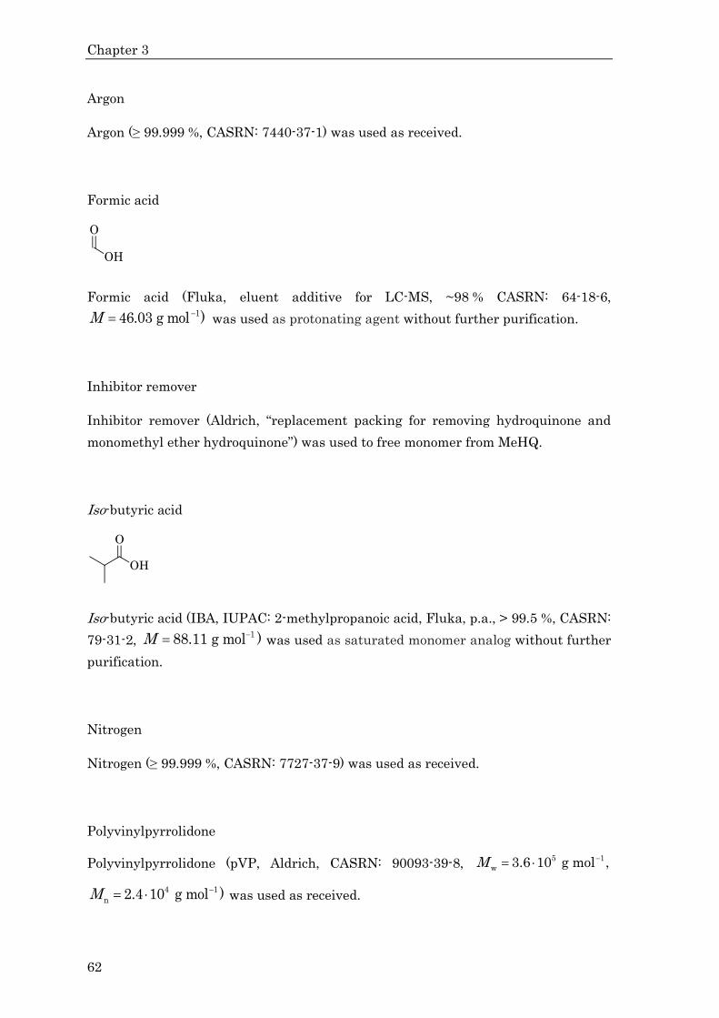
Chapter 3

62

Argon

Argon (≥ 99.999 %, CASRN: 7440-37-1) was used as received.

Formic acid

Formic acid (Fluka, eluent additive for LC-MS, ~98 % CASRN: 64-18-6, 146.03 g mol )M was used as protonating agent without further purification.

Inhibitor remover

Inhibitor remover (Aldrich, “replacement packing for removing hydroquinone and

monomethyl ether hydroquinone”) was used to free monomer from MeHQ.

Iso-butyric acid

Iso-butyric acid (IBA, IUPAC: 2-methylpropanoic acid, Fluka, p.a., > 99.5 %, CASRN:

79-31-2, 188.11 g mol )M was used as saturated monomer analog without further

purification.

Nitrogen

Nitrogen (≥ 99.999 %, CASRN: 7727-37-9) was used as received.

Polyvinylpyrrolidone

Polyvinylpyrrolidone (pVP, Aldrich, CASRN: 90093-39-8, 5 1

w 3.6 10 g mol ,M

4 1

n 2.4 10 g mol )M was used as received.


63

Sodium chloride

Sodium chloride (Merck, p.a., > 99.5 %) was used as received.

3.2 Purification Procedures

Monomers may come into contact with ground glass joints during purification and

storage. In order to reduce impurities, PTFE rings (Dr. Dietmar Glindemann,

GlindemannTM PTFE sealing rings) were used instead of grease to seal ground glass

joints and PTFE stopcocks were used for column chromatography. The chemical

substances were stored according to instructions of supplier. Monomer free of

inhibitor was stored at 20 °C.

Inhibitor Remover

Inhibitors that are more polar than the monomer can be removed by passing the

mixture through a column filled with inhibitor remover. By this procedure MeHQ-

free BA of was obtained.

Distillation

In order to remove impurities, e.g., inhibitor, monomer was distilled over a 20 cm

Vigreux column at 8 mbar. Fine copper wire was placed in the still pot and the lower

parts of the column to prevent polymerization. This is especially important for AA.

3.3 NIR

3.3.1 Setup

Spectra were recorded with the FTIR spectrometer IFSTM 88 (Bruker Optik). A

water-cooled cell holder was used to reduce heat transfer from the cell to

spectrometer components. The optical system was permanently purged with

compressed air, dried by an adsorption dryer (ZANDER Aufbereitungstechnik). The

Chapter 3

64

optical configuration consisted of a tungsten halogen lamp (Gilway Technical Lamp,

L7417A, 12 V, 50 W), a silicon-coated calcium difluoride beam splitter (model

T8401), and a liquid-nitrogen-cooled InSb detector (InfraRed Associates, model

D413, 1 mm in diameter). The sample compartment was separated from the optical

system by calcium difluoride windows.

Cuvettes were connected to the heated/refrigerated circulating bath F3-K (Haake)

operated with an aqueous ethane-1,2-diol solution (50 percent by volume) used as

heat transfer fluid.

Data acquisition and data analysis were performed using the software OPUS

(Bruker Optik, version 4.2 or 6.0).

3.3.2 Thermally initiated Polymerization in a Cuvette

All components were mixed and filled into a cylindrical, thermostated optical cell

(65.14/Q, optical path length, if not stated otherwise 10 mm, Spectrosil, Starna) and

purged with argon for 4 minutes. The cell was positioned into the spectrometer (v.s.)

and brought to the desired temperature. The time required for heating to

polymerization temperature was in most cases shorter than the inhibition period.

This initial range of negligible degree of monomer conversion was cut off in the

conversion-time profiles, which were subjected to modeling. A few reaction mixtures

led to significant degree of monomer conversion before the final temperature had

been reached. Change in temperature was checked via the shape of the broad water

peak (v.i. Figure 3-2.). In these particular cases the data points from before final

temperature were removed and the remaining profile was extrapolated to correct the

time. These profiles were not used for modeling, but only to compare with the

predictions of the final model. NIR spectra were taken in short intervals (of 3 to 60 s)

until monomer conversion was complete, which took up to several hours. The

absence of residual monomer was additionally checked by 1H-NMR .

Cleaning of the cell can become tedious, especially for measurements without CTA.

Leaving the devices for extended time periods (several hours to days) in saturated

3NaHCO solution turned out to be the best method for precleaning them.


65

3.3.3 Photoinitiated Polymerization in a Cuvette

All components were mixed and filled into a cylindrical, thermostated optical cell

(Starna 65.14/Q/ optical path length, if not stated otherwise 10 mm, SpectrosilTM,

Starna). D1173 was used as photoinitiator. The initial mixture was purged with

argon for 4 minutes. After heating to reaction temperature, the polymerizing

mixture was irradiated for 40 to 80 s with an Osram Ultra-VitaluxTM 300 W lamp

positioned at a distance of 18 cm, until a degree of monomer conversion of a few

percent had been reached, which was monitored via NIR spectroscopy (v.s.).

Polymerization was stopped by adding MeHQ to the reaction mixture, which was

afterwards cooled to –20 °C.

3.3.4 Degree of Monomer Conversion

6300 6200 6100 60000.0

0.1

0.2

0.3

0.4

ab

sorb

an

ce

wavenumber / cm1

Figure 3-1 NIR absorbance spectrum showing the signal of the first overtone of the C–H

stretching recorded during a polymerization of 0.11 g g1 AA in D2O. The arrow

indicates the direction of change with reaction time. Only the peak around 1175 cm1

is used for calculation of conversion.

Chapter 3

66

The first overtone of the C–H-stretching mode at the C=C double bond was used to

quantitatively measure degree of monomer conversion as a function of

polymerization time. This method works in both organic and aqueous

solutions.[130,140,141] A typical set of lines for different degrees of monomer conversion

(from zero to full) during AA polymerization is depicted in Figure 3-1.

5550 5540 5530 55200.600

0.625

0.650

0.675

0.700

ab

sorb

an

ce

wavenumber / cm1

room temperature

65 °C

Figure 3-2 Shown is a part of the broad water signal also depicted in Figure 3-3 for a series of

spectra taken every 15 s during the initial period of a polymerization of 0.11 g g1 AA

in D2O. The arrow gives the direction of change with time. Final temperature is

reached approximately after the fourth spectrum.

For AA, the absorbance of the C–H mode was integrated between 6250 and

6120 1cmagainst a baseline fitted via a polynomial passing through the absorbance

data points at 6370, 6280, 6113 and 6085 1cm .

Ionization of monomer shifted the

signal. For NaA, the absorbance of the C–H mode was integrated between 6261 and

6053 1cmagainst a baseline fitted via a polynomial passing through the absorbance

data points at 6284, 6255, 6062 and 6051 1cm .

For MAA, the absorbance of the C–H

mode was integrated between 6275 and 6092 1cm against a baseline fitted via a

polynomial passing through the absorbance data points at 6310, 6274, 6088 and

6065 1cm .

As the shift resulting from ionization is not very strong and other


67

influences might interfere, the NIR signal was not used to calculate the degree of

ionization of monomer for different degrees of conversion.

The polymer signal (C–H-stretching mode at the saturated carbon atom) is much

weaker and positioned at smaller wavenuber (Figure 3-3 c) compared to the

corresponding monomer signal. The low wavenuber region of monomer peak overlaps

to a small extent with high wavenuber region of the polymer peak (Figure 3-3 d). As

not the full but rather the high wavenuber part of the signal was used, this did not

affect the data evaluation described above.

As shown in Figure 3-2, the shape of the broad peak associated with water is

especially sensitive towards temperature. Such being the case, the water peak was

used to check temperature and ensure that only data points were used after final

temperature was reached. Moreover, it was secured that reaction enthalpy of

polymerization did not lead to significant temperature increase and the whole

process remained isothermal.

For the purpose of improving signal-to-noise quality, 2D O was used as the solvent

instead of 2H O. [141] For a typical monomer weight fraction of

10.1 g g the monomer

signal is just a small peak on the flank of the 2H O peak (Figure 3-3 a), whereas the

background absorption of 2D O is at smaller wave numbers than the one of

2H O in

the =C–H region under investigation (Figure 3-3 b).

No notable solvent isotope effect on the polymerization kinetics is expected to

occur.[141] This assumption has been verified by comparison with reported conversion

vs. time profiles for 2H O being the solvent.[90] In recipes of PREDICITM simulation

weight was corrected by ration of densities taken from ref.[142]

7000 6000 50000.0

0.5

1.0

1.5

2.0

2.5

3.0

3.5

7000 6000 50000.0

0.5

1.0

1.5

2.0

2.5

3.0

3.5

7000 6000 5000

0.00

0.25

0.50

0.75

7000 6000 50000.0

0.5

1.0

1.5

2.0

2.5

3.0

3.5

dcb

a

ab

sorb

an

ce

wavenumber / cm1

Figure 3-3 Typical NIR spectra.with important lines being marked: dark blue square: H2O; medium blue square: D2O; red circle: monomer; green triangle:

polymer; conditions: a: 0.10 g g1 AA in H2O, optical path 2 mm; b: 0.11 g g1 AA in D2O, low conversion, optical path 10 mm; c: same as b, but full

conversion; d: difference between b and c


69

3.4 EPR

3.4.1 Setup

EPR spectra were recorded on an EPR CW/Transient Spectrometer System Elexsys-

IITM 500T (Bruker Biospin) or an ElexsysTM E500 (Bruker Biospin) both operating

with the X-band. The resonator, Optical Transmission Cavity (Bruker), was open or

equipped with a grid, to allow for irradiation. Temperature was set by a 4131VT unit

(Bruker) purging the sample cavity with nitrogen.

Samples were irradiated inside the cavity by a 500 W mercury arc lamp (LAX 1450,

Müller Elektronik; HBO 500 W/2, Osram). It was checked that spectra taken with a

cut-off filter WG335 (Schott) had the same ratio of EPR line intensities. As the

weaker UV radiation with filter impaired S/N ratio, samples from measurements

without filter were used for data processing.

3.4.2 Organic Samples

Monomer in solvent was by several freeze-pump-thaw cycles and CTA in solvent

was degassed by several freeze-pump-thaw cycles as well .The following preparation

was carried out in a glove-box under an argon atmosphere. Then the two solutions

were mixed giving a monomer concentration of 11.52 mol L with either

10.02 mol mol , i.e. 13.04 mmol L, or

10.05 mol mol , i.e. 17.60 mmol L, and an

initiator concentration of 116 mmol L. An EPR quartz tube of 5 mm outer, and 4 mm

inner diameter (Bruker) was filled with 200 L reaction mixture. The sample tube

was closed with a plastic cap and sealed with PARAFILMTM. The samples were

measured directly afterwards to avoid side reactions, e.g., the thiol-ene reaction

occurred.

Optimized measuring conditions were: single scan: 83.9 s, width: 100 G; time

constant: 10.24 ms; attenuation: 13; receiver gain: 60; microwave power: 10 mW;

modulation amplitude: 3 G.

Chapter 3

70

3.4.3 Aqueous Samples

Measuring EPR in water is especially challenging. A special EPR-cell constructed for

measurements in water was used, the ER 165FCVT-S-Q, also called WG-808-S-Q,

(WilmadLabGlass/Rototec-Spintec) made of SuprasilTM to guarantee a clean

background. The measuring section is between two planar plates maximizing the

filling factor. It has a volume of 150 L and is filled completely. No liquid is left

above this section as this would reduce S/N-ratio. D1173 (initiator) weight fraction

was 3 14.7 10 g g .

Optimized measuring conditions were: single scan: 10.0 s, width: 100 G; time

constant: 0.01 ms; attenuation: 13; receiver gain: 70; microwave power: 10 mW;

modulation amplitude: 3 G.

3.4.1 Deconvolution of Spectra

Spectra were simulated using SimfoniaTM v.1.25 (Bruker). Coupling constants and

line broadening were first adjusted for spectra measured at temperatures where one

radical species dominates, i.e. SPRs at 50 °C and MCRs at 70 °C. Simulation of the

spectra was carried out by Dr. Tatiana Sergeeva. For details see ref.[101]

The simulated spectra were used to fit the complex spectra applying ExcelTM solver

and gain fraction of different radical species.

3.4.2 Calibration

Radical concentrations were obtained by calibration with TEMPO. The double

integral of the signal and radical concentration are correlated linearly. The double

integral of spectra at different concentrations of TEMPO are plotted against radical

concentration and fitted to a straight line, the slope of which is the calibration

constant. It has to be measured for each composition of the reaction mixture and

temperature. This is only possible for BA-toluene mixtures, because ME and TEMPO

undergo a redox reaction. Calibration with TEMPO was carried out by Dr. Johannes

Barth. For details see ref.[143,144]


71

Spectra were subjected to double integration to obtain absolute radical concentration

by multiplying with the calibration constant. In principle, both the measured

spectrum and the fitted spectrum should yield the same result. However, the

baseline has to be corrected. It can be straight and just tilted, but also slightly

curved. The more lines in a spectrum the more difficult it is to correct the baseline

without erasing signal.

Analysis of SPR dominated spectra (few lines) gave the same result for original and

simulated spectra. Analysis of spectra with many lines from both SPR and MCR

gave lower radical concentration for measured (and baseline-corrected) spectra. As

this could be traced back to signal being cut off, simulated spectra were used for

analysis.

3.5 NMR

1H-NMR spectra were recorded in thin-walled tubes (e.g. Schott S, NorellTM 508-up)

at solute mass concentrations of about 10.06 g g .

Spectra for qualitative analysis

were determined at room temperature with an AvanceTM III (300 MHz, Bruker). In

order to improve S/N-ratio, 16 or 32 FIDs were co-added.

Spectra for quantitative 1H-NMR analysis were determined by a UnityTM 300 or

MercuryTM 300 (300 MHz, Varian).

3.5.1 Quantitative 1H-NMR

Optimum 1H-NMR measuring conditions for quantitative analysis were taken from

Schrooten.[145] The relaxation of the hydrogen atom attached to the -carbon is

unusually slow. Baseline (Bernstein polynomial fit) and phase (manual) were

corrected.

Chapter 3

72

Table 3-1 Optimum conditions for quantitative 1H-NMR measurement.VI Ref.[145]

parameter AA pAA

measuring temperature 35 °C

pulse angle 10° 84°

repetitions 32

acquisition time / s 3.128

relaxation delay / s 3 5

3.5.2 Quantitative 13C-NMR

FIDs were processed by the MestReNovaTM software package. Baseline (Bernstein

polynomial fit or multipoint baseline correction) and phase (manual) were corrected.

Exponential apodization of the FID was done to improve S/N. It was checked for the

samples that exhibit a rather intense quaternary carbon peak that apodization does

not influence the results.VII

Spectra for quantitative 13C-NMR analysis were determined with an Inova 500

equipped with a cryo-probe (500 MHz, Varian). Because of the cryo-probe, as it is

oversaturated in the very beginning of recording, backward linear prediction (up to

22 points, Toeplitz) was necessary.

VI NMR measurements were performed at the Institut für Organische und

Biomolekulare Chemie (Georg-August-Universität Göttingen) by R. Machinek.

VII Apodization may cause higher intensity for peaks of atoms with a shorter relaxation time.


73

Figure 3-4 Typical FID of a 13C-NMR of pAA.

Optimum 13C-NMR measuring conditions for quantitative analysis were determined

in this work. Different measuring parameters were tested. A sample with very high

branching was chosen (polymerization conditions: 10.1 g gAA,

10.02 g gVA-086, in

water, 170 °C, X = 85 %) to abtain a good S/N-ratio.

The two questions were, which delay is needed to get complete relaxation of all

crucial nuclei, and which delay is necessary for the nuclear Overhauser effect, NOE,

built up during acquisition, to recede. In order to minimize NOE, measurement was

carried out with inverse gated decoupling, i.e. it was only decoupled during

acquisition. Different combinations of acquisition time, at, and relaxation delay, rd,

were tried. Acquisition should not be too long because of NOE built-up, on the other

hand not too short, because otherwise signal might be cut off and this to a different

extent for different nuclei. Thus, looking at the FID, shown in Figure 3-4, the value

should not be smaller than 0.5 s and not bigger than 1.0 s. The relaxation delay

should be so long further extension thereof has no more influence. To allow for

shorter delays, the pulse angle was reduced.

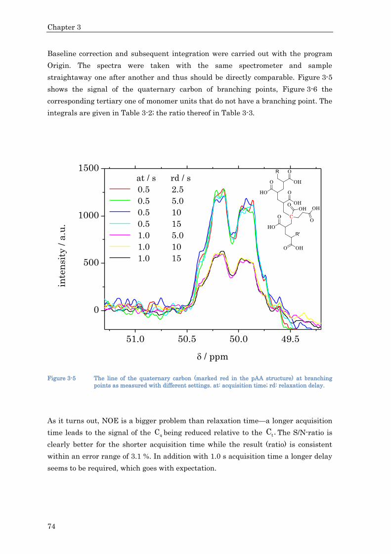
Chapter 3

74

Baseline correction and subsequent integration were carried out with the program

Origin. The spectra were taken with the same spectrometer and sample

straightaway one after another and thus should be directly comparable. Figure 3-5

shows the signal of the quaternary carbon of branching points, Figure 3-6 the

corresponding tertiary one of monomer units that do not have a branching point. The

integrals are given in Table 3-2; the ratio thereof in Table 3-3.

51.0 50.5 50.0 49.5

0

500

1000

1500

inte

nsi

ty /

a.u

.

/ ppm

at / s rd / s

0.5 2.5

0.5 5.0

0.5 10

0.5 15

1.0 5.0

1.0 10

1.0 15

Figure 3-5 The line of the quaternary carbon (marked red in the pAA structure) at branching

points as measured with different settings. at: acquisition time; rd: relaxation delay.

As it turns out, NOE is a bigger problem than relaxation time—a longer acquisition

time leads to the signal of the qC being reduced relative to the tC . The S/N-ratio is

clearly better for the shorter acquisition time while the result (ratio) is consistent

within an error range of 3.1 %. In addition with 1.0 s acquisition time a longer delay

seems to be required, which goes with expectation.


75

Summing up, an acquisition time of 0.5 s gives a better signal and requires only a

relaxation delay of 2.5 s. Therefore, these measuring conditions are the optimal ones,

summarized in Table 3-4.

44.8 44.6 44.4 44.2 44.0 43.8 43.6

0.0

5.0x103

1.0x104

1.5x104

2.0x104

2.5x104

3.0x104

3.5x104

at / s rd / s

0.5 2.5

0.5 5.0

0.5 10

0.5 15

1.0 5.0

1.0 10

1.0 15

inte

nsi

ty /

a.u

.

/ ppm

Figure 3-6 The line of the tertiary carbon (marked red in the pAA structure), at which branching

points can occur, as measured with different settings. at: acquisition time; rd:

relaxation delay.

Table 3-2 Integrals of the peaks shown in Figure 3-5 and Figure 3-6.

measuring condition range / ppm Integral / a.u. Deviation / %

at 0.5 rd 2.5 50.50 - 49.60 612.1 0.99

at 0.5 rd 5.0 50.50 - 49.60 599.8 -1.04

at 0.5 rd 10 50.50 - 49.60 639.1 5.44

at 0.5 rd 15 50.50 - 49.60 606.1 0.00

Chapter 3

76

at 1.0 rd 5.0 50.50 - 49.60 320.2 5.82

at 1.0 rd 10 50.50 - 49.60 345.1 14.05

at 1.0 rd 15 50.50 - 49.60 302.6 0.00

at 0.5 rd 2.5 44.60 - 43.60 10 436.2 -0.87

at 0.5 rd 5.0 44.60 - 43.60 10 236.1 -2.77

at 0.5 rd 10 44.60 - 43.60 10 368.6 -1.51

at 0.5 rd 15 44.60 - 43.60 10 527.9 0.00

at 1.0 rd 5.0 44.60 - 43.60 4 847.0 -4.74

at 1.0 rd 10 44.60 - 43.60 5 036.9 -1.01

at 1.0 rd 15 44.60 - 43.60 5 088.2 0.00

Table 3-3 Ratio of the integrals of the peaks shown in Figure 3-2 and Figure 3-3.

measuring condition ratio quaternary to

tertiary line

deviation from

ratio of 0.5 rd 15 s / %

at 0.5 rd 2.5 0.055 1.8

at 0.5 rd 5.0 0.055 1.7

at 0.5 rd 10 0.058 6.6

at 0.5 rd 15 0.054 0.0

at 1.0 rd 5.0 0.062 13.8

at 1.0 rd 10 0.064 17.8

at 1.0 rd 15 0.056 3.1


77

Table 3-4 Optimum conditions for quantitative 13C-NMR measurement of pAAVIII

Pw 0.3 often not possible due to viscosity and

homogeneity issues

measuring

temperature 50 °C or higher

decoupling n n y decoupling with an NOE as low as possible

pulse angle 36° compromise between maximum intensity and a

measuring time as short as possible

repetitions

640

14208

for highly branched polymer

for sample with minimal branching

acquisition time 0.5 s

relaxation delay 2.5 s

3.5.3 Polymerization in NMR Sample Tube

The reaction mixture was filled into an NMR tube and purged with argon through a

hollow needle for 6 minutes. The sample tube was closed with a plastic cap and

sealed with PARAFIMTM. The tube was kept in the heated/refrigerated circulating

bath F3-K (Haake) operated with an aqueous ethane-1,2-diol solution (50 percent by

volume) used as heat transfer fluid for the desired time. The polymerization was

quenched by addition of MeHQ and oxygen (air) plus cooling to 0 °C (ice bath).

VIII NMR measurements were performed at the Institut für Organische und Biomolekulare

Chemie (Georg-August-Universität Göttingen) by R. Machinek.

Chapter 3

78

3.6 Density Measurement

A density meter based on the oscillating U-tube principle was used. It consists of a

data acquisition unit, DMA 60 (Anton Paar), a measuring unit, DMA 602TP (Anton

Paar), and a high-temperature cell, DMA 602 H (DURANTM 50, −10 ≤ ≤ 150 °C,

Anton Paar). Temperature monitoring inside the U-tube was carried out by means of

a digital thermometer (Voltcraft 302 K/J Thermometer). Heating was performed by a

water bath circulator (Haake, D2-L). To reduce overheating, the water bath

circulator was connected to a water circulation cooler (Lauda Dr. R. Wobser,

WK 500).

The measurement is only correct, if the U-tube is filled completely and there are no

bubbles inside it. This became a problem especially for measurements a higher

temperature, because solubility of gases decreases. Therefore, solutions were first

heated to desired temperature and filled into the capillary afterwards.

3.7 Viscosity Measurement

If not stated otherwise, viscosity was measured by an AMVnTM instrument (Anton

Paar GmbH) using RheoplusTM (Anton Paar GmbH) as the analysis software. It is a

falling/rolling sphere viscosimeter, which uses four different capillaries to cover a

range from 0.3 to 20 000 mPa s. The capillaries were filled by sucking in the solution

into it with a syringe from the other end.IX

In a few experiments, kinematic viscosity, , was measured with an Ubbelohde

viscometer (SCHOTT, 0a, inside diameter of 0.53 mm) and corrected via the

Hagenbach–Couette procedure. The viscometer was mounted inside a clear-view

thermostat (Lauda Dr. R. Wobser, D40) filled with water. It remained inside for at

least 900 s before measurement to allow for thermal equilibration. The water

temperature was determined by a Pt100 connected to a PID controller (Eurotherm,

2460). The PID controller regulated a universal relay box (Lauda Dr. R. Wobser, R3),

which controlled the power supply of an immersion heater.

IX Some of the viscosity and density measurements were carried out by Roman Kremring

during his bachelor thesis.


79

Dynamic viscosities, , were determined via combination of the measured kinematic

viscosity and density, , by:

3.7.1 Important Features of Polymer Solutions

0 5000 10000 15000 20000

45

50

55

60

/

mP

a s

time / s

Figure 3-7 A sample of 0.06 g g1 pMAA was measured at 25 °C by an AMVn (falling/rolling

sphere viscosimeter) two times. First, the capillary was filled quickly and with high

sheer force (red stars), second, the capillary was filled gingerly with lower sheer force

(blue triangles). The arrow indicates three singular measurements, during which a

tiny bubble in the capillary slowed the sphere down hence giving a too high value of .

Polymer solutions are non-Newtonian fluids, viz., when stressed they become either

less viscous over time (thixotropy), or they become more viscous over time

(3.1)

Chapter 3

80

(rheopecty). Both the Ubbelohde viscometer and the falling/rolling sphere

viscosimeter cause sheer forces on the sample during filling and measuring. For the

latter these can be minimized by choosing a small angle, thus slowing down the

sphere. If not stated otherwise, viscosity was measured at an angle of 20°. Figure 3-7

shows how the filling procedure increases viscosity and it slowly decreases

afterwards. Therefore, the sheer forces during measurement are very small, if the

right conditions have been chosen. Filling the capillary gingerly reduces

sheer-induced rise in viscosity. Nevertheless, it takes time for viscosity to decrease.

Samples were filled and left for 18 000 to 25 200 s before measurement. Another

problem is occurrence of bubbles as they slow down or even block the movement of

the sphere. Measurements that gave indication of bubbles or other interferences

were discarded. Bubbles became a problem especially for measurements a higher

temperature, because solubility of gases decreases. For that reason, solutions were

first heated to desired temperature and filled into the capillary afterwards.

3.7.2 Polymerization in Viscosity Measurement Capillary

All components were mixed, purged with argon for 8 minutes, and directly sucked

into the measuring capillary by a syringe at the other end. The capillary was

positioned into the viscosimeter (v.s.) and brought to the desired temperature.

Initiators that produce gas, e.g., azo-initiators are unsuitable for this experiment. A 10.05 g g monomer solution changes density by less than 1 %, this effect was

ignored.

3.8 Preparation of Buffer Solutions

Buffer solutions were prepared based on ref.[146] Main components, e.g., citric acid,

were chosen following the recipe given. Aqueous solutions 1(1.0 mol L )

of sodium

hydroxide or hydrochloric acid, respectively, were added under stirring until the

desired pH value had been reached. During this process, the pH value was

monitored online.


81

3.9 SEC

The entire set of size-exclusion chromatography, SEC, analysis was carried out in

aqueous phase by I. Lacík, DSc, and M. Stach, PhD, and co-workers at the Polymer

Institute of the Slovak Academy of Sciences according to procedures detailed

elsewhere.[59,91,147]

3.10 ESI-MS

The polymer was dissolved, e.g., in water/ethanol to give a solution of ca. 10.1 g L .

Two spectrometers were used to measure ESI-MS.X

An Ion-trap LCQTM (Thermo Finnigan) connected to an HPLC setup (v.i.) was

operated with an electrospray voltage of 4.5 kV and a capillary temperature of

200 °C. It had a measuring range of 200–2000 m/z. In order to improve S/N-ratio ca.

200 spectra were coadded.

A micrOTOFTM (Bruker) was operated with an electrospray voltage of 3.8 kV and a

capillary temperature of 180 °C. It had a measuring range of 30–3000 m/z. In order

to improve S/N-ratio ca. 200 spectra were coadded.

Spectra were analyzed by OriginProTM 8.5 (OriginLab).

3.11 HPLC

Setup

The high-performance liquid chromatography, HPLC, setup consisted of an AS

1555TM autosampler (Jasco), degasser 3492 (Kontron), a 57 SynergiTM MAX RP

column (Phenomenex), and a SurveyorTM PDA UV-detector (Finnigan) operating

X ESI-MS analysis was performed at the Institut für Organische und Biomolekulare Chemie

(Georg-August-Universität Göttingen) by Dr. H. Frauendorf.

Chapter 3

82

from 200 to 800 nm.XI The HPLC setup was connected to an ESI-MS spectromter

(Finnigan, Ion Trap LCQTM), v.i.

Sample preparation

Aqueous samples with 11 mg g XII initiator were stirred until dissolution was

complete. They were kept at the desired temperature for a defined time analogously

to either polymerization in a heating block or polymerization in a tubular reactor

(v.i.). In the latter case, residence time was corrected analogously to polymerization

(v.i.). Afterwards samples were cooled down rapidly in an ice bath.

Measurement

The injection volume was 5 L, the flow rate 5 L 1s . The starting eluent was water

with 4 15 10 g g formic acid. Within 900 s the eluent changed gradually to methanol

with 4 15 10 g g formic acid. Eluation was continued with the latter for 420 s.

The signal appertaining to non-decomposed initiator could be assigned to a line

found after 360 s via ESI-MS. Integration of the corresponding UV signal gave the

concentration of the initiator.

3.12 pH-Meter

A S47 SevenMulti™ dual meter pH / conductivity (Mettler-Toledo,

−2.000 ≤ pH ≤ 20.000, 0.001 S cm−1 ≤ c ≤ 1 000 mS cm−1) was used to determine as

pH values.

XI HPLC analysis was performed at the Institut für Organische und Biomolekulare Chemie

(Georg-August-Universität Göttingen) by Dr. H. Frauendorf. XII For some samples a higher initial weight fraction was chosen and the samples were

diluted prior to HPLC measurement.


83

3.13 High-Temperature Polymerizations

Figure 3-8 The setup for high temperature experiments is shown schematically. It could be

operated in two modes.

Figure 3-8 depicts the setup schematically.XIII The reaction mixture started from the

reservoir container located on a balance (Omnilab, OL 3100-P), which was connected

to a computer to calculate mass flow in 1 s intervals. The reaction mixture flowed via

a PTFE tube (inner diameter 1 mm) to the degasser (Ercatech AG, ERC-3215α) and

further to an HPLC pump (built by the mechanical workshop of the Institut für

Physikalische Chemie, Georg-August-Universität Göttingen). The pump gave a

pressure of 200 bar and from here on connection was by a stainless steel capillary

(AD: 1/16´´) with an inner diameter of 0.5 mm. Then it entered a double line tube

(1 m) to get a temperature of 50 °C., which was not enough to induce significant

monomer conversion but reduced temperature difference to reaction temperature. In

the next step the reaction mixture flowed into the tubular reactor located in a

heating bath (Haake, N3) filled with silicone oil. The stainless steel, tubular reactor

consisted of two 510.1156 (Nova Swiss, AD: 1/16´´, ID: 0.5 mm). It was spiral-shaped,

had a length of 1050 cm, an inner diameter of 0.5 mm ± 0.05 mm, and thus a

geometric volume of 2.06 mL ± 0.41 mL. Temperature was measured by CIA S250

Chromel/Alumel thermocouple and pressure by a P3MB (HBM). Afterwards the

reaction mixture was cooled to 50 °C in a double line tube (1 m). Then it flowed into a

high-pressure cell (described in more detail elsewhere[145,148]) heated electrically to

50 °C and located in the FTIR spectrometer IFS 88 (Bruker Optik). A controlling

XIII The high-temperature polymerizations were all carried out by Daniel Weiß.[148] under

cosupervision of Dr. H.-P. Voegele.

Chapter 3

84

valve followed to set the velocity of the flow. The last part of the setup was a

collecting vessel.

The setup allowed for two different modes of operation described in what follows.

3.13.1 Stopped-Flow experiments in High-Pressure Cell

The tubular reactor was bypassed and polymerization took place in the high

pressure cell. The reaction mixture flowed without prior warming through the cell

until stationary condition was reached. Then the valves of the high-pressure cell

were closed and the cell was used as a batch reactor. Polymerization was followed by

NIR as described in subchapter 3.3. The upper temperature limit for measurements

with this mode of operation was set by initiator decay. At temperatures above

140 °C, VA-086 decayed so fast that significant X had already been reached at the

starting point.

With this setup, it was not possible to draw samples during polymerization.

The procedure is described in more detail here.[148] .

3.13.2 Polymerization in a Tubular Reactor

Polymerization was carried out inside the tubular reactor. Residence time, , was set

by flow rate and was calculated from mass flow, density of the reaction mixture and

geometric volume of the reactor. This theoretical value had to be corrected (v.i.).

The lower and upper temperature limits for measurements with this mode of

operation were set by initiator decay. At temperatures above 170 °C, VA-086 decayed

so fast that high final monomer conversion was reached even at the highest flow

rate. Measuring a conversion vs. time profile is not possible under these conditions.

At temperatures below 130 °C, VA-086 decayed so slowly even for the lowest flow

rate, which still allowed for turbulent flow, high conversion could not be reached.

Samples were taken at each flow rate. They were dried in vacuo at temperatures up

to 90 °C and measured by NMR (subchapter 3.5.1 and 3.5.2).


85

Correction of residence time in the tubular reactor

0 10 20 30 40 500.00

0.03

0.06

0.09

0.12

in

ten

sity

/ a

.u.

time / s

Figure 3-9 Residence time distribution of the whole setup (red) and without the tubular reactor

(blue) measured as time-dependent signal intensity (pulse-response) for residence time

experiments applying marker (AA) as approximate delta function.

Residence time of the tubular reactor was measured by flowing water through the

apparatus with and without the reactor being included. AA was injected as marking

substance as an approximate delta function. Increase of the center peak of the

interferogram (to increase time resolution) was used to measure the arrival of

marking substance. The result is shown in Figure 3-9.

The curves from experiments with the tubular reactor have, within experimental

accuracy, the same shape as the curves from experiments without the tubular

reactor—there is only a time offset. Thus, no significant broadening by the high-

pressure cell can be observed.

The curves were integrated to obtain , see Figure 3-10. The true residence time of

the tubular reactor was calculated as the difference between residence time

including the tubular reactor and residence time not including the reactor.

Chapter 3

86

0 10 20 30 40 500.0

0.2

0.4

0.6

0.8

1.0

F(t

)

time / s

Figure 3-10 Sum functions of the curves shown in Figure 3-9. This is used to compute the true

residence time of the tubular reactor as the difference between residence time

including the tubular reactor (red) and residence time not including the reactor (blue).

This was done for different flow rates and the residence time calculated from mass

flow, density of the reaction mixture and geometric volume of the reactor. This

theoretical value, calc , was plotted against the true residence time, . This is shown

in Figure 3-11. A linear relationship was found and an empirical correction function

was determined, eq. (3.2), with which all experimental results given later have been

corrected.

The procedure is described in more detail elsewhere.[148]

calc/ s / s 2.38 4.58 (3.2)


87

3.0 4.5 6.0 7.5 9.00

4

8

12

16

/

s

calc

/ s

Figure 3-11 Calculated and directly measured residence times are compared (green squares).

These values are fitted to a straight line (red, eq. (3.2)).

As it was only possible to measure for high flow rates, for lower flow rates, and

thus higher conversion, residence time was corrected via linear extrapolation,

eq. (3.2). The time has to be more precise for the beginning of the polymerization, as

the rate of polymerization is highest here. The comparison of the conversion-time

profiles of polymerization with the stopped-flow operation to conversion-time profiles

from polymerization in the tubular reactor before and after correction suggest that

the correction and even the extrapolation works well. An example is given in

Figure 3-12. Small symbols give the result from batch polymerization (stopped-floe

operation) used as reference here. Big open symbols belong to a polymerization of the

same reaction mixture in the tubular reactor. The rate of polymerization seems to be

smaller for the tubular reactor. Correction of residence time of the tubular reactor

via eq. (3.2) yields the big, solid symbols. The corrected conversion-time profile of the

polymerization in the tubular reactor agrees with the one of the batch reactor, thus

the rates of polymerization are the same.

Chapter 3

88

0 50 100 150 2000.0

0.2

0.4

0.6

0.8

1.0

X

time / s

Figure 3-12 Conversion-time profiles of polymerization with the stopped flow operation (small

symbols) is compared to conversion-time profiles from polymerization in the tubular

reactor before correction (big open symbols) and after correction (big filled symbols) are

compared. 0.1 g g1 AA was polymerized with 0.002 g g1 VA-086 in H2O at 140 °C.

3.14 Other Setups for Polymerization

3.14.1 1 L Automated Reactor

A LabMaxTM 1 L automated, stirred reactor (Mettler-Toledo) was connected to a

nitrogen cylinder and operated by iC Software (Mettler-Toledo).

A mixture of water and monomer was stirred under a nitrogen blanket for 1800 s

and heated to desired temperature. Then initiator and, if required, CTA were added

in countercurrent. Samples were drawn in increasing time intervals. They were

cooled immediately after having been taken from the polymerizing mixture and both

MeHQ and oxygen (air) were added. The decay of monomer and CTA concentrations

was monitored by 1H-NMR and by gravimetric analysis.


89

3.14.2 Polymerization in a Heating Block

The reaction mixture was filled into a dark (protection from UV light) twist-off-glass

with a septum integrated in the cap. Argon was purged through the reaction mixture

by a hollow needle. The sample was kept in the Block Heater 250 (Rotilab) for the

desired time. In order to ensure good mixing, the heater was standing on a KS-15

shaker (Edmund Bühler GmbH)

Polymerization was stopped either by cooling the sample rapidly with liquid

nitrogen, which sometimes caused the glass to break, or by adding MeHQ and

oxygen (air) and cooling the sample in an ice bath.

3.14.3 Polymerization in a Flask

The reactor was a flask connected to a Schlenk line. A mixture of water and solvent

was either purged with argon for 30 minutes or degassed by several freeze-pump-

thaw circles and flooded with argon afterwards. It was brought to desired

temperature. Then dissolved initiator and, if required, CTA were added by a syringe

through a septum. Samples were drawn in increasing intervals. They were cooled

immediately after having been taken from the polymerizing mixture and both MeHQ

and oxygen (air) were added.

Later, this procedure was replaced by polymerization in a lined flask, which allows

for better temperature control.

Synthesis of arylic acid macromonomer

The above described procedure was modified to synthesize arylic acid

macromonomer, MM(AA).

150 mL DMSO were purged with argon and brought to 138 °C. 0.0116 g VA-086 was

dissolved in 5.3 g DMSO. Half of the initiator solution was added through a syringe.

10.72 g AA was added dropwise. The rest of the initiator was added slowly. After

2400 s the reaction mixture was cooled in an ice bath. No inhibitor was added. The

product of extraction from water was dried in vacuo.

Chapter 3

90

190 mL o-Xylol were purged with argon and brought to 140 °C. 0.116 g DTBP was

added through a syringe, then 10.79 g AA. After 8700 s the reaction mixture was

cooled in an ice bath. No inhibitor was added. The reaction product was dried in

vacuo.

3.14.4 Polymerization in a Lined Flask

The reactor was a lined flask with its hose barbs connected to a heated/refrigerated

circulating bath (Haake, F3-K) with ethanol used as heat transfer fluid. The flask

was completely covered with aluminum foil. The reaction mixture was purged with

argon for 2400 s and brought to the desired temperature. The foil was opened on one

side and the flask was irradiated by a 100 W mercury arc lamp (LAX 100, Müller

Elektronik; HBO 100 W/2, Osram) from ca. 40 cm distance. Afterwards a sample was

drawn by a wide, hollow needle, cooled immediately to 20 °C, and stored in

darkness. This procedure was repeated until final conversion was reached.

3.15 Computer Programs

3.15.1 Curve Fitting

Fitting of mathematical functions to experimental data was conducted by the

software OriginProTM 8.5 (OriginLab), except for curve fitting described in 3.15.2.

Linear fitting is carried out applying the method of least squares. For non-linear

curve fitting the Levenberg–Marquardt algorithm is used for iterative adjustment of

parameters.

3.15.2 Determination of Joint Confidence Regions

The program Contour (A. M. van Herk, version 1.8) was used to generate ellipses

corresponding to joint confidence regions for Arrhenius activation energy and

Arrhenius pre-exponential factor of p.k The details of the program are given

elsewhere.[149,150]


91

3.15.3 Simulation

Simulations were performed by the program PrediciTM v6.4.8 (Dr. Michael Wulkow

Computing in Technology GmbH).

3.16 Error Estimate

Density

The density meter is specified to be accurate to 6 31.5 10 g cm .

ESI-MS

Results are from the LCQTM are precise by 0.1 m/z and results from the micrOTOFTM

are precise by 0.005 m/z.

Monomer Concentration from FT—NIR

Repeated recording of spectra of the same sample shows slightly different results.

Errors may be introduced by apodization and phase correction, but the main source

of error seems to arise from uncertainties of the baseline.

The error of the integrated absorbance is estimated to be less than ±2 %, but rises for

very low concentrations.

NMR

As correct measuring conditions were checked and results from different data

processing were compared, values derived by 1H-NMR are estimated to have at least

two significant digits and those from 13C-NMR to have at least one significant digit.

pH

The inaccuracy of the pH values is given by the manufacturer to be ±0.002.

Statistical Error

The errors of parameters which are deduced by curve fitting are determined using

statistical methods. They are mostly given together with the respective value in the

text.

Chapter 3

92

Temperature

For experiments in cuvettes as well as for viscosity determination, an error of

±0.5 °C is estimated on the basis of manufacturer’s information. The temperature in

the pH measurements is precise to ±0.1 °C. The temperature in density

measurements is accurate within ±0.1 °C. The temperature in the nitrogen flow to

thermostat EPR tubes is precise to ±0.1 °C.

Viscosity

The error given by manufacturer of the AMVn is: accuracy (trueness) < 0.7 %,

precision < 0.35 %. The accuracy of the other viscosity measurements is slightly

lower.

Weight

For preparing the reaction solutions and gravimetric analysis, an analytical balance

(CPA 3245, Sartorius) with an accuracy of ±0.1 mg was used.


93

Methacrylic Acid

95

4

4 Methacrylic Acid

The polymerization of MAA (methacrylic acid, IUPAC: 2-methylpropenoic acid) is of

industrial interest as the product is widely used, most often as comonomer for

polymers applied, e.g., in hygiene and cosmetics. These polymers are produced by

radical polymerization in aqueous phase. In addition to solution polymerization,

emulsion polymerizations are performed in which carboxylic monomers such as

methacrylic acid may act as in-situ stabilizer. Moreover, MAA is similar to AA, but

the kinetics are simpler due to lack of backbiting. Knowledge about MAA kinetics

may help to better understand AA kinetics. For modeling polymerization in aqueous

solution, detailed kinetic and mechanistic knowledge is required.

The propagation rate coefficient is known from PLP–SEC analysis.[5,89,151] SEC on

pMAA may be performed after quantitative methylation of the carboxyl moieties

yielding PMMA[57,90] or directly on pMAA via aqueous-phase SEC.[91] The pk value of

MAA varies enormously as a function of both monomer concentration and degree of

ionization[9,11,58,59,91,92] e.g., decreases by about one order of magnitude in passing

from dilute aqueous solution of non-ionized MAA to either bulk polymerization of

non-ionized MAA or to fully ionized MAA in dilute solution. These effects are not

independent of each other, i.e., the variation of pk with monomer content is weaker

with partially ionized MAA and may even be reversed with fully ionized MAA.[11] It

has been attempted to model solution and emulsion polymerization from = 0 to

= 1.[79] PLP–SEC studies on samples, to which pMAA had been added, thus

mimicking situations of different degrees of monomer conversion, establish that it is

Chapter 4

96

essentially the ratio of MAA-to-water concentrations which is responsible for the

characteristic dependence of pk in aqueous-solution.[9]

For non-ionized MAA, both the SP–PLP–NIR[121] and the SP–PLP–EPR

techniques[120] have been applied in aqueous solution. The experimental pk and tk

values turned out to be well suited for modeling aqueous-phase MAA polymerization

kinetics and polymer molar mass distribution in the absence of efficient chain

transfer.[90]

So far, modeling of MAA polymerization in aqueous solution has not been addressed

at technically relevant CTA concentrations. This chaper describes polymerization

kinetics and modeling of MAA with a special focus on chain transfer. Unlike to

preceding investigations,[90] the chain-length dependence of kt has to be explicitly

taken into account and the impact of CTA concentration on the variation of

termination rate with degree of monomer conversion has to be accounted for as well.

Parts of this chapter have already been published:

Wittenberg, N. F. G.; Buback, M.; Stach, M.; Lacík, I. Macromol. Chem. Phys. 2012,

213, 2653–2658.

Wittenberg, N. F. G.; Buback, M.; Hutchinson, R. A. Macromol. React. Eng. 2013, 7,

267–276.

4.1 Chain-Transfer to 2-Mercaptoethanol

Modeling polymerization under the influence of chain-transfer requires knowledge of

the corresponding rate coefficients. Therefore, the chain-transfer constant of

2-mercaptoethanol for methacrylic acid polymerization in aqueous solution has been

measured for varying MAA content from 0.05 to 10.3 g gat 50 °C. The analysis has

been carried out via both the Mayo and the chain length distribution, CLD,

method.XIV

Another question to be answered is, whether trk in aqueous solution varies with

MAA content as does pk or stays constant as is the case with conventional

XIV CLD stands for chain length distribution, while CLDT stands for chain-length dependent

termination. While a little confusing, these are the common abbreviations in literature.

Methacrylic Acid

97

monomers in organic solvents. It turns out that CTAC is independent of monomer

concentration. Thus, tr,CTAk exhibits the same strong decrease with monomer

concentration as has been reported for p .k

The question was easier to answer with ME being the CTA, as the associated CTAC

is large and may be accurately measured.[28,152] Non-ionized MAA was selected as

monomer, because pk is already known.[9,59] Moreover, in contrast to acrylate-type

monomers, where secondary chain-end radicals may undergo backbiting reactions to

produce tertiary midchain radicals, in MAA polymerization only one type of

propagating radical occurs. The simultaneous presence of these two types of radicals

adds complexity to the kinetic analysis,[33,101,153] as addressed in chapter 5.

4.1.1 Chain Transfer Constants deduced by the Mayo Method

0.00 0.02 0.040.000

0.002

0.004

0.006



cME

/ cMAA

Figure 4-1 Mayo plot of product from polymerization of 0.30 g g1 MAA at 50 °C in aqueous

solution at different levels of photoinitiator (D1173): 1.31 mmol L1 (red),

6.56 mmol L1 (black), and 32.8 mmol L1 (green). The corresponding best fits to a

straight line are given as dotted lines and the concatenate fit as blue solid line. Due to

dominance of chain transfer as chain stopping event, the individual slopes are almost

identical.

Chapter 4

98

The Mayo method requires polymerizations to be dominated by chain transfer as

stopping event. In order to demonstrate the fulfillment of the necessary conditions,

polymerizations were carried out at different initiator concentrations, but otherwise

identical conditions. The result of the Mayo procedure, eq. (2.12), yielding CTAC is

shown in Figure 4-1 for the three different initiator concentrations. Five times more

and five times less initiator content than used for the other experiments presented

later resulted in almost the same slope of the Mayo plot.

0.00 0.02 0.040.000

0.002

0.004

0.006



n

cME

/ cMAA

nn

M

Mi

M

wn

M2

Mi

M

Figure 4-2 Inverse of the number average degree of polymerization for pMAA samples plotted as

a function of the ratio of CTA (here ME) to monomer (here MAA) content. Polymer was

produced by reaction to low degrees of monomer conversion for 0.30 g g1 MAA in

aqueous solution at 50 °C and 6.56 mmol L1 D1173 added as photoinitiator; data

points are either deduced from Mn (red squares) or from Mw (blue circles). The dotted,

red line is fitted to the data from Mn (eq. (4.1)) and the straight, blue line is fitted to

the data from MW (eq. (4.2)).

The number-average degree of polymerization, ni , may be deduced either from nM

or wM . The quality of nM determination may be affected by uncertainties of SEC

analysis at lower molar masses. It thus appeared recommendable to determine nM

from wM , the value of which is accessible with better accuracy than nM . In case of

Methacrylic Acid

99

transfer-controlled polymerization, as with ME being the CTA, dispersity w n/M M is

close to 2, which allows for an estimate of nM from wM .[23,29]

Figure 4-2 shows a typical Mayo plot for MAA polymerization in aqueous phase with

ni being deduced from SEC curves either via eq. (4.1) or via eq. (4.2).

3 4 5 6

cME

/cMAA

= 0.030

cME

/cMAA

= 0.020c

ME/c

MAA = 0.013

lg (M / g mol

)

w (

lg (

M /

g m

ol))

*

Figure 4-3 Shown are three typical MMDs of polymer produced by reaction to low degrees of

monomer conversion for 0.15 g g1 MAA in aqueous solution at 50 °C, cME/cMAA = 0.013

(dashed line) 0.020 (solid line) 0.030 (dotted line), and 6.56 mmol L1 D1173. The MMD

represented by a dotted line has a second maximum marked by an asterisk. This

occurred only for a few samples of polymerizations with high ME content and was

probably caused by posterior initiation by ME. The thiol-ene reaction as a possible

mechanism of initiation is shown at the top. Analysis was still possible (see text).

nn

M

Mi

M (4.1)

wn

M2

Mi

M (4.2)

Chapter 4

100

The data from both nM and wM are in close agreement, which demonstrates the

quality of SEC analysis and also suggests that w n/M M is close to 2, as is expected in

case of chain transfer to ME being the dominant chain-terminating event. As the

scatter on the data from wM is smaller, only these numbers have been fitted by the

straight line. From the slope to this line CTAC = 0.116 ± 0.010 is obtained. According

to the same procedure, CTAC has been determined for other MAA weight fractions

and photoinitiator concentrations. The so-obtained numbers are listed in Table 4-1.

Using wM for analysis has an additional advantage. Among the Mayo data a few

results of polymerizations with high ME concentration are included where the

MMDs of the pMAA samples were bimodal probably from subsequent initiation by

ME (see Figure 4-3). As water evaporates faster than MAA and ME, the

concentration of both latter species increase during drying and the thiol-ene reaction

(Figure 4-3 top) may become important. For these MMDs, the data points obtained

from nM (eq. (4.1)) deviate from a straight line deduced by fitting the values of

monomodal MMDs only. This does not hold true for fitting via eq. (4.2). The so-

obtained 1

ni

values all closely fit to a straight line. This is shown in Figure 4-4.

0.00 0.02 0.04

0.00

0.01

0.02

1

cME

/ cMAA

Figure 4-4 Mayo plot of polymer produced by reaction to low degrees of monomer conversion for

0.15 g g1 MAA in aqueous solution at 50 °C. Data points are either deduced from Mn

(red squares) or from Mw (blue circles); the blue line is fitted to the data from MW

(eq. (4.2)). Data points corresponding to bimodal MMDs are marked by an arrow.

Methacrylic Acid

101

4.1.2 Chain Transfer Constants deduced by the CLD Method

The CLD method estimates CTAC according to eq. (2.14), which requires the slope of

the ln MP vs. M plot, eq. (2.13), to be known. SEC yields the weight fraction of

polymer of molar mass M, .Mw From Mw the quantity

MP is obtained via

eq. (4.3).[154]

0.0 2.0x105

4.0x105

6.0x105

8.0x105

-28

-24

-20

-16

Mw

Mn

ln (

PM

)

M / g mol

Figure 4-5 CLD plot for determination of the chain-transfer constant according to eq. (4.3) and

(4.4); the data refers to polymer produced by reaction to low degrees of monomer

conversion for 0.30 g g1 MAA in aqueous solution at 50 °C, cME/cMAA = 0.007, and

6.56 mmol L1 D1173 being added as the photoinitiator; the slope to the straight line is

used for determination of the chain-transfer constant CCTA (see Figure 4-6). The region

of fitting is indicated by solid line. Mn and Mw are given for orientation.

2

MM

wP

M (4.3)

Chapter 4

102

The so-obtained ln MP vs. M correlation for pMAA from polymerization of

0.30 g g1 MAA in aqueous solution at 50 °C is shown in Figure 4-5. Straight-line

behavior is not seen over the entire range of pMAA masses. According to eq. (2.13),

the data for very high molar mass should be considered for deducing the slope , in

particular in cases where termination becomes significant.[23,29] The resulting

dilemma is illustrated in Figure 4-5 by indicating the positions of nM and wM ,

which are in the region of maximum signal intensity. In this region, molar mass is

not sufficiently high as to allow for determination of the chain-transfer constant. On

the other hand, the very high molar mass region, e.g., above 500 000 1g mol , is too

poor in signal quality as to provide a reliable estimate of the slope The CLD

method has thus been applied in this example to molar masses around

400 000 1g mol (Figure 4-5, solid line), to which the straight line is fitted. In general,

the region used was a compromise between choosing the highest molar masses, and

still having sufficient signal intensity. The region of maximum RI intensity is not

suitable for CLD analysis in this example.

An example of a final plot yielding CTAC from the CLD method is depicted in

Figure 4-6.

2ln λMw

MM

(4.4)

Methacrylic Acid

103

0.00 0.02 0.040.000

0.002

0.004

0.006

(M

M)

cME

/ cMAA

Figure 4-6 The asterisk symbols represent the results from CLD fitting according to eq. (4.4). The

dotted line represents the slope taken from the Mayo plot in Figure 4-2 for the same

experimental conditions: 0.30 g g1 MAA in aqueous solution at 50 °C, and

6.56 mmol L1 D1173 . This line has almost identical slope as one from fitting the

asterisk symbols to a straight line, which yields CCTA from CLD method (Table 4-1).

The data point marked by the arrow is the one deduced from the slope to the fitted line

in Figure 4-5.

4.1.3 Comparison of Mayo and CLD methods

Data obtained for CTAC from the CLD method are represented by the asterisk

symbols in Figure 4-6. The results from the Mayo procedure (see Figure 4-2) are

given by the dotted line. The CLD results exhibit a significantly larger scatter than

the Mayo ones. The CTAC values from the two procedures are compared in Table 4-1.

Within the larger scatter of the CLD data, good agreement between the Mayo and

CLD method is found. The uncertainty is slightly larger at the lowest MAA content

(0.05 1g g). It should further be noted from Table 4-1 that the CLD method yields

unusually high CTAC at the largest photoinitiator concentration, which is most likely

due to the occurrence of smaller radicals and thus to a larger impact of termination

Chapter 4

104

affecting CLD analysis. With the exception of this particular CTAC value, the data in

Table 4-1 indicate that CTAC at 50 °C is more or less independent of both MAA and

photoinitiator concentration. The bottom entry in Table 4-1, lists the result from an

experiment at 90 °C. Comparison with the associated experiment at 50 °C tells that

the Mayo and CLD methods yield opposite trends for the temperature effect on CTAC ,

which may be understood as an indication of CTAC not being dependent on

temperature to a significant extent, as expected (see subchapter 2.3.1). The Mayo

method appears to provide simple but accurate access to the transfer constant in

case of high CTA activity with polymerization in aqueous solution.

0.0 0.1 0.2 0.3

0.25

0.50

0.75

1.00

1.25

wMAA

CCTA

/ C

CTA,w = 0.05

kp / k

p,w = 0.05

Figure 4-7 Relative CCTA and kp (with respect to the associated value for wMAA = 0.05). The

CCTA/CCTA(wMAA = 0.05) data refers to MAA polymerization at 50 °C, blue triangles

pointing right: Mayo method, aqua triangles pointing left: CLD method. The data

points scatter more for lower concentrations. The kp data is taken from ref.[59,121]

The essential result of the present study is illustrated in Figure 4-7, in which both

CTAC and pk are plotted relative to the respective values at 10.95 g g .MAAw Whereas

CTAC is independent of monomer content, pk exhibits the well-known strong

decrease upon enhancing MAA concentration. This observation says that the

genuine kinetic effect associated with hindrance to rotational motion in the

Methacrylic Acid

105

transition state structure by the molecular environment is primarily due to

characteristics of the radical chain-end and thus is more or less identical for

propagation and for transfer to the CTA. The important consequence of this finding

is that the known enormous variation of pk with monomer concentration, and thus

with conversion, also applies to chain transfer, which may easily be taken into

account by adopting constant CTAC for a wide range of monomer concentration. This

finding probably holds for other transfer reactions, e.g., transfer to monomer, as

well. It was found for modeling MAA polymerization in aqueous solution that

transfer to monomer had to be included and both the tr p/ constantk k and the

tr constantk approach were tested.[90] The first approach gave a slightly better

representation of the experimental MMDs, although, within experimental accuracy

it was not possible to decide whether the rate coefficient of transfer is affected in the

same way by the monomer-to-water ratio as is pk . The findings of the present work

indicates that the tr p/ constantk k approach is correct.

Table 4-1 Chain-transfer constants, CCTA, of ME in MAA polymerizations in aqueous solution at

different MAA concentrations, cMAA, and initiator concentrations, cD1173, at 50 and

90 °C deduced via the Mayo and the CLD method. The uncertainties are estimated as

twice the statistical error of each underlying experimental series. The weighted mean

value were calculated.

CTAC (Mayo)

CTAC (CLD)

variation of 1

MAA / mol Lc

(50 °C, 1

D1173 / mmol L 6.56c )

0.600 (5 wt.%) 0.138 ± 0.015 0.10 ± 0.03

1.80 (15 wt.%) 0.125 ± 0.024 0.12 ± 0.04

3.60 (30 wt.%) 0.116 ± 0.010 0.12 ± 0.05

mean value 0.12 ± 0.01 0.11 ± 0.02

variation of D1173c / mmol L1

(50 °C, 1

MAA / mol L 3.60c )

1.31 0.122 ± 0.006 0.13 ± 0.75

6.56 0.116 ± 0.010 0.12 ± 0.05

32.8 0.121 ± 0.014 0.19 ± 0.02

mean value 0.12 ± 0.01 0.18 ± 0.02

variation of temperature / °C

(1

MAA / mol L 0.600,c 1

D1173 / mmol L 6.56c )

50 0.138 ± 0.015 0.10 ± 0.03

90 0.110 ± 0.030 0.13 ± 0.02

Chapter 4

106

4.2 Model development for Non-ionized Methacrylic Acid

Batch radical polymerization of non-ionized methacrylic acid, 10.1 0.3 g g in

aqueous solution, has been studied between 35 and 50 °C at ambient pressure with

2-mercaptoethanol as the chain-transfer agent. Initial polymerization rate decreases

with CTA concentration, which has been varied up to CTA M/ 0.24.n n In order to

illustrate the influence of CTA, three conversion vs. time profiles of polymerizations

with different level of CTA content (but otherwise identical conditions) are depicted

in Figure 4-8.

Kinetic modeling is presented, which includes chain-length-dependent termination

and uses an empirical function to account for the dependence of termination rate on

both monomer conversion and molar mass of the polymeric product. In conjunction

with PREDICITM simulation, these models afford for an adequate representation of

the measured monomer conversion vs. time profiles and MMDs.

The kinetic models consider initiation, propagation, termination, transfer to

monomer and transfer to a CTA. Using a highly efficient CTA, such as ME, reduces

chain length to an extent that requires the dependence of tk on radical chain length

and on the molar mass (distribution) of the produced polymer to be taken into

account.

The reaction scheme is presented in Table 4-2, where I2 represents the initiator,

which decays thermally with the rate coefficient dk and exhibits a growth efficiency,

f, of primary radicals I . Within a first addition step, a growing chain P of length

unity is formed from I and one monomer molecule M. The radical chain grows by

addition of monomer molecules with the rate coefficient p .k Termination of two

radicals may occur via combination, with rate coefficient tck , producing a (dead)

macromolecule D, or via disproportionation, which proceeds with rate coefficient tdk

by hydrogen transfer and results in the formation of two macromolecules. Chain

growth also ceases upon transfer to monomer or to a CTA. The chain length of

polymeric species is given by the indices i, j, or 1. Radical species are marked by a

dot, e.g., P .i

The values of the individual rate coefficients, are summarized in Table

4-3 and Table 4-4, respectively

Methacrylic Acid

107

0 5000 10000 150000.00

0.25

0.50

0.75

1.00

cME

/cMAA

= 0.03

0.3 g g1

MAA

no CTA cME

/cMAA

= 0.002X

time / s

cME

/cMAA

= 0.2

Figure 4-8 Polymerization of 0.30 g g MAA in aqueous solution with 0.001 g g V-50 as initiator

at 50 °C. The relative CTA content is given for each profile in the graph.

The azo-initiator V-50 was used, as peroxides and thiols may form a redox initiation

system.[155] Moreover, initiator decay should be independent of pH, which is the case

with V-50.[156] V-50 decomposes according to a first-order rate law with a half-life of

about 10 hours at 50 °C.[156] This slow initiator decay ensures almost constant

initiator content during the reaction and avoids dead-end polymerization. Initiator

efficiency was assumed to be f = 0.8, which is a typical value that has successfully

been used for modeling.[90] The variation of density was considered in the simulation

by assuming ideal mixing. The temperature dependence of the density of monomer

and solvent was fitted by a third-order and a second-order polynomial,

respectively.[157]

It was checked that the thiol-ene reaction does not play a significant role for the

systems under investigation.

Chapter 4

108

Table 4-2 Individual reaction steps used for modeling radical polymerization of non-ionized

methacrylic acid in aqueous solution.

initiator decomposition d

2I 2If k

chain initiation p

1I M Rk

propagation p

1R M Rk

i i

termination

by combination tcR R P

k

i j i j

by disproportionation tdR R P P

k

i j i j

chain

transfer

to monomer tr,M

1R M P Rk

i i

to CTA tr,CTA

1R CTA P Rk

i i

The variation of pk as a function of initial MAA weight fraction,

0

MAAw , of degree of

monomer conversion, X, and of temperature, is known from literature; p,maxk in

Table 4-3 refers to propagation in highly diluted aqueous solution.[121] There are

indications of pk being chain-length dependent up to i = 10.[118] This dependence

needs to be considered under conditions of extreme chain transfer, as with catalytic

chain-transfer agents.[49] For the present system no need for incorporation of this

effect was found.

CTAC for ME is 0.122, with this number being insensitive towards MAA-to-water

content and temperature (4.1). Transfer to monomer is known from literature[90] and

as CTAC was found to be constant, the same was assumed for M .C

xx The fraction of termination by disproportionation, , was assumed to be 0.8,

which is a typical value for methacrylates.[90] The composite model is used for

representation of chain-length-dependent termination. Information about tk as a

function of MAA concentration and of radical chain length is available from SP–

PLP–EPR experiments.[120] To avoid the high computational effort associated with

considering individual reactions between two radicals of chain lengths i and j,

respectively, termination is scaled via the number-average radical size. The chain-

length dependence of tk has been implemented into PREDICITM via the composite

Methacrylic Acid

109

model with the relevant chain length being given by the number-average size. This

procedure is associated with only modest additional computational effort.

This procedure is based on the fact that tk averaged over all chain lengths, tk ,

has been shown to be equal to the tk of the average chain length of that distribution,

ni , times a correction factor, d , which is usually close to unity as given in

eq. (4.5).[107,158-161] The correction factor results from the fact that shorter chains

contribute more to overall termination. Eq. (4.5) is valid in case of termination being

dominant.

In case of transfer being dominant eq. (4.5) transforms into eq. (4.6) yielding almost

the same result.[161]

Beyond chain-length dependence, the variation of tk with monomer conversion has

to be incorporated. Such information is available from SP–PLP–NIR measurements.

Within the present study, the effects of chain length and conversion on termination

rate are both taken into account to allow for simulation of MAA polymerization in

aqueous solution within a wide range of CTA concentrations and up to complete

degrees of monomer conversion.

l l2

d

l l

2 2 2

2 2 1

(4.5)

2

d l1 (4.6)

l0

t t dnk k i

(4.7)

Chapter 4

110

4.2.1 Modeling Polymerization at Medium initial Monomer Content

The entries in Table 4-3 demonstrate that a large body of kinetic information on

MAA radical polymerization in aqueous MAA solution is available from independent

experiments. It is essentially termination kinetics at different levels of ME

concentration, which remains to be determined via simulation of the experimental

monomer conversion vs. polymerization time data. Under conditions of highly

efficient chain transfer, e.g., with ME, the distributions of radical size and of polymer

molar mass are controlled by propagation and transfer rates.

104

105

106

107

108

l = 0.166

l = 0.160

ic = 68

ic = 100

s = 0.61

<k

t> /

L m

ol s

Mn(R) / g mol

s = 0.62

Figure 4-9 Dark blue squares: Initial kt values deduced as mean values from the conversion range

0 < X < 0.025 of MAA polymerizations (0.30 g g in aqueous solution) at varying cME/cM

up to 0.2. The abscissa values are simulated number-average values of growing

polymer chains. Solid blue line: fitting according to the composite model; data points

for Mn below 5852 g mol–1 were used for fitting the short-chain behavior, whereas data

at higher average molar masses are subjected to fitting the long-chain behavior. Red

dashed line: kti,i and s from SP–PLP–EPR work on MAA;[120] pink dashed line:

extrapolation with ic of MAA and l from theoretical considerations.[106,119]

To determine the effect of radical chain length on tk without interference of

contributions from polymer-induced viscosity changes, rates at different ME

Methacrylic Acid

111

concentrations and low degrees of monomer conversion, i.e., below 2.5 percent were

estimated under the assumption of tk being independent of monomer conversion.

The so-obtained tk values are plotted as a function of the number-average size of

growing polymer chains, with these latter values being deduced from simulation. A

double-log plot of the resulting tk vs. the number-average radical size is shown in

Figure 4-9. CTA concentration has been widely varied which results in the broad

range of radical sizes.

In addition to tk from simulation of measured MAA conversion vs. time traces

(open square symbols), values of ,

t

i ik deduced from SP–PLP–EPR experiments[120]

are represented by the dashed line in Figure 4-9. The EPR experiment is highly

instationary, but refers to a narrow distribution of radical chain lengths.

Termination occurs between two radicals of approximately the same size, which

increases linearly with time t after pulsing. The square symbols refer to termination

under stationary conditions with the reacting radicals exhibiting a broad

distribution of chain lengths. The number-average size of radicals, nM , is obtained

as the mean value over a broad distribution of radical sizes, whereas the abscissa

value for the SP–PLP–EPR data refers to a narrow distribution of radical chain

lengths. In view of this fundamental difference, the data from the two experiments

are remarkably close to each other in slope, thus in s , but also in absolute value.

The close comparison also holds for ,

t

i ik extrapolated to longer radical chain lengths,

which values are illustrated by the pink dashed line in Figure 4-9. This line is

constructed by adopting the cross-over chain length of methyl methacrylate (MMA)

for MAA and taking the power-law exponent l from theory.[106,119]

From SP–PLP–EPR, the value of s for MAA was determined to be 0.62 ± 0.06,[120]

which is close to s 0.61, the corresponding number from the present study. It

should however be noted that the latter s is based on only three data points. For

MMA bulk polymerization, s has been obtained from SP–PLP–EPR measurements

to be 0.63 [103] and from RAFT-CLDT to be 0.65.[119] So far, no value of either ci or l

has been measured for MAA by the SP–PLP–EPR technique because of poor signal

intensity.[120] The values for MMA are close to ci = 100[107] and l = 0.16.[106] The

corresponding numbers deduced within the present study from the <kt> vs. Pn

correlation in Figure 1 are: c 68i and l 0.17.

In Figure 4-9, an offset is seen between the dashed and the solid line, which

corresponds to 1,1

tk from stationary experiments being by a factor of 0.7 below the

SP–PLP–EPR value. However, according to theory,[161] this factor should be 1.27

(calculated from eq. (4.6), eq. (4.5) gives 1.12). Closer inspection tells that the two

lines correspond to different systems, 10.1 g g MAA in H2O and

10.3 g g MAA in

Chapter 4

112

D2O both at 50 °C. Viscosity measurements for these two solutions at ambient

pressure resulted in the values 0.6681 and 1.2064 mPa s, respectively. The

associated ratio of viscosities is 0.554. In conjunction with the theoretical factor of

1.27 the ratio of 1,1

tk values thus should be 0.554 ∙ 1.27 = 0.704, which is in perfect

agreement with the measured difference. The close comparison demonstrates the

dominant effect of viscosity on 1,1

tk .

The satisfactory agreement of the two types of tk representations (Figure 4-9)

provides support for applying the composite model to the correlation of the low

conversion chain-length-averaged termination rate coefficient with average radical

chain length, ni , according to the full line in Figure 1. Below nM = 5852 g mol,

which corresponds to ci = 68, the expression for short-chain radicals, eq. (4.8), has

been used, whereas eq. (4.9) has been applied for long-chain radicals. In what

follows, tk always refers to the chain length averaged rate coefficient; for reasons of

convenience, chevrons are omitted.

After focusing on CLDT, the variation of termination rate with monomer conversion

will now be addressed. At low degrees of monomer conversion, segmental diffusion

(SD) operates, which is controlled by the viscosity of the monomer-solvent mixture.

Over an initial range of monomer conversion, the associated coefficient t,SDk remains

more or less constant which results in a plateau value of tk up to moderate degrees

of monomer conversion. At higher conversion, tk starts to clearly decrease, as

termination transitions to translational diffusion control with the associated rate

coefficient t,TDk scaling with the inverse viscosity of the polymerizing medium. This

type of bulk viscosity includes the impact of the concentration and of the type of

polymer produced during the course of a particular polymerization. t,TDk is expressed

in terms of 0

t,TDk , the hypothetical termination rate coefficient under translational

diffusion control prior to polymerization, and of r , the relative viscosity, 0

r /

with 0 referring to the viscosity of the initial solution prior to polymerization.

Towards even higher conversion, center-of-mass diffusion of macroradicals

s1,1

t,CLD t n n c k k i i i

(4.8)

l ls l1,1 0

t,CLD t c n t n n c k k i i k i i i

(4.9)

Methacrylic Acid

113

essentially ceases and termination runs under reaction-diffusion (RD) control, which

assumes two radical sites to approach each other by propagation of the chain ends in

conjunction with mobility of chain segments. Termination under RD conditions thus

scales with pk via the reaction-diffusion constant, RDC , which is enhanced by chain

flexibility. The t,TDk expression of the present study into solution polymerization

uses monomer concentration, eq. (2.41). At very high conversion and thus high

viscosity even propagation may run under diffusion control. (see subchapter 2.4.5)

The variation of relative viscosity has been described by an exponential relation

containing one single parameter C .[90] Adopting this notation and assuming pk not

to run under diffusion control, turns eq. (2.43) into eq. (4.10), which has been

successfully applied for modeling MAA polymerization in aqueous solution.[90]

For an initial MAA content of 10.6 g g, the plateau value of constant (but chain-

length dependent) t,SDk holds up to about 0.1.X For an MAA content of 10.3 g g,

the region of constant t,SDk is approximately twice as large and extends up to

0.2X with these ranges, however, being affected by the size and the structure of

produced pMAA.[121]

As no backbiting occurs during MAA polymerization, ideal polymerization kinetics,XV

eq. (2.7), has been used for estimating tk as a function of X from experimental

monomer conversion vs. time data of all experiments.

Figure 4-10 illustrates tk data deduced via eq. (2.7) for two polymerizations in the

absence of CTA. The different regions of diffusion control, i.e., by SD, TD, and RD

are clearly seen. Also presented in Figure 4-10 are conversion vs. time profiles

measured at two ME levels. The initial plateau region which is assigned to SD,

increases with ME content and extends over the entire experimental conversion

range at the highest ME concentration. At ME MAA/ 0.2c c , the plateau value for

termination under SD control is significantly above tk at lower ME content. The tk

plateau value for MAA polymerization with ME MAA/ 0.002c c is close to the one for

XV Here, ideal refers to each single data point, i.e., overall constancy is not assumed.

Moreover, CLD-T is not excluded.

*

t RD p

0

t,SD t,TD

11

1 eX C

k C X k

k k

(4.10)

Chapter 4

114

MAA polymerization without CTA. The conversion range of SD control is however

larger than in the absence of ME. Moreover, the decline of tk in the TD region is less

pronounced. The data for chemically induced MAA polymerization with

ME MAA/ 0.002c c is remarkably close to tk deduced from SP-PLP-NIR experiments

on 10.3 g g MAA in aqueous solution without CTA.[121] The reason behind this

agreement probably is that the high radical concentration, which is instantaneously

produced by the laser pulse, leads to similarly low molar masses as in chemically

induced polymerizations with ME MAA/ 0.002c c .

0.0 0.2 0.4 0.6 0.8

5

6

7

8

0.3 g g1

MAA

CI, no CTA (two experiments)

CI, 0.002 cME

/cMAA

SPPLPNIR

log(k

t / L

mol s

)

X

SD

TD

RD

CI, 0.2 cME

/cMAA

Figure 4-10 Dependence of the termination rate coefficient on monomer conversion as derived from

ideal polymerization kinetics (eq. (2.7)) for four chemically initiated (CI)

polymerizations (0.30 g g in aqueous solution) at ambient pressure; data points were

smoothed; the asterisk symbols are data from SP–PLP–NIR experiments

(wMAA0 = 0.30 g g, 50 °C, 2000 bar),[121] which were extrapolated to ambient pressure

with eq. (2.25) via the activation volume of 12.4 cm3 mol. The ME concentrations are

given in the Figure. The notations SD, TD, and, RD refer to control of termination by

segmental, translational (centre-of-mass), and reaction diffusion, respectively.

Eq. (4.11) has been conceived as an expression for tk , in which chain-length

dependence and conversion dependence are merged together. Aspects of conversion-

dependent s [120] and l

[108] have already been discussed. Most studies into CLDT

Methacrylic Acid

115

refer to low monomer conversion, whereas studies into the conversion dependence

ignore CLDT. No clear indications for a potential dependence of s and of l on

monomer conversion were found. Hence, both power-law exponents are assumed to

be insensitive towards monomer conversion. In eq. (4.11), the parameters t,SDk and 0

t,TDk are replaced by t,CLD t,SD/sd k k and by 0

t,CLD t,TD/td k k . The parameters sd and

td account for the relative contributions of segmental diffusion and translational

diffusion:

Transformation of eq. (4.11) into eq. (4.8) and eq. (4.9), respectively, requires:

sd + td = 1 for X = 0. Analysis of the individual monomer conversion vs. time profiles

by fitting to eq. (4.11) via the Levenberg-Marquardt algorithm yields numbers for sd,

td, C , and RDC . The parameters sd = 0.96 ± 0.01 and td = 0.04 ± 0.01 turned out to

provide an adequate representation of tk for the entire set (10.3 g g MAA) of

measured conversion vs. time traces. The conversion dependence of termination rate

on ME concentration is exclusively assigned to C . The impact of ME content is thus

contained in t,CLDk and in C . The parameter RD 20C was deduced from

polymerization rates measured in the absence of ME. This value is in reasonable

agreement with the one of MMA, for which *

RDC = 93.5 was measured, which

corresponds to RD 10.3C .[130] Assuming pk to be independent of chain length results

in t,RDk being also insensitive toward chain length.

Illustrated in Figure 4-11 are the individual contributions of the terms in eq. (4.11)

to overall tk for MAA polymerization (10.3 g g) in aqueous solution without CTA

being present. t,CLDk remains essentially constant over the wide conversion range, in

which average chain-length drops only by a factor of 2.6. Up to about X = 0.6, the

first term on the RHS eq. (4.11) dominates and RD plays no significant role. Above

0.74, t,RDk exceeds the first term.

η1

t t,CLD RD M peX C

k k sd td C c k

(4.11)

Chapter 4

116

0.0 0.3 0.6 0.9

5

6

7

kt without k

t,RD

kt as realized

in model

log(k

t / L

mol s

)

X

SD

TD

RD

kt,CLD

kt,RD

Figure 4-11 Contributions to overall kt according to eq. (4.11) as a function of degree of monomer

conversion. The notations SD, TD, and, RD refer to control of termination by

segmental, translational (centre-of-mass), and reaction diffusion, respectively.

The parameter C may be deduced by PREDICITM fitting of the entire body of

polymerization data for a wide range of molar masses, which may be achieved by

variation of CTA content. In Figure 4-12 the so-obtained C values are plotted as a

function of the weight average molar mass at X = 0.5, a value which is close to the

mean molar mass taken over the entire conversion range. The entire set of

experimental C vs. wM data is fitted by eq. (4.12) which results in the parameter

values a = 1.4 and b = 0.15. Interestingly, this value for b is similar to the power-law

exponent for self-diffusion of polymer in good solvents (see subchapter 2.4.4) and

thus also similar to l .

w

bC a M (4.12)

Methacrylic Acid

117

Combination of eq. (4.11) and eq. (4.12) replaces C by a and b. Thus, by using one

additional parameter, an adequate representation of the measured conversion vs.

time traces at widely different polymer molar masses is achieved.

The combined influence of wM of dead polymer in solution and chain length of

macroradicals (long-chain region) on tk is depicted in Figure 4-13 top. The weight of

the former is at 0.5X much stronger. wM and X have the same influence on tk

shown in Figure 4-13 bottom.

104

105

106

6

8

10

12

C

Mw (P) / g mol

0.15

w 1.4 4.1 2 C M

t t,CLD RD M p

1 4.11

e

X C

k k C c ksd td

Figure 4-12 Correlation of Cwith the weight-average molar mass of pMAA produced up to X = 0.5

at different levels of chain-transfer agent ME. The symbols are deduced from

PREDICITM fitting of experimental conversion-time data. The obtained fit parameters

refer to eq. (4.12), which extends eq. (4.11).

Illustrated in Figure 4-14 is the impact on tk of ME concentrations up to

ME MAA/ 0.2c c according to eq. (4.11) and eq. (4.12). The minor increase of tk upon

enhancing monomer conversion at the highest ME content results from a weak

decrease of radical chain length towards lower MAA content, i.e., toward higher

Chapter 4

118

conversion. In addition to the logarithm of tk , the square root of tk is plotted (in the

lower part of Figure 4-14). The inverse of the latter quantity scales with both rate of

polymerization and kinetic chain length.

The quality of the kinetic model associated with the rate coefficients summarized in

Table 4-3 is illustrated by comparison of measured and simulated monomer

conversion vs. time traces in Figure 4-15. The model turns out to adequately

represent the polymerization kinetics of 10.3 g g MAA in aqueous solution at 50 °C

for ME contents between zero and ME MAA/ 0.2c c . For 0, 0.05 and 0.1 ME content,

repeat experiments are included. They demonstrate that the quality of simulation is

close to experimental reproducibility. At high monomer conversion, the model

slightly overestimates polymerization rate, which may be partly due to reduced

initiator efficiency or to diffusion control of pk at very high viscosity. These

phenomena are not included in the model.

Methacrylic Acid

119

Figure 4-13 The dependence of kt on molar mass of polymer in solution and chain length of

macroradicals at X = 0.5 is plotted at the top. The dependence of kt on molar mass of

polymer in solution and degree of monomer conversion at <in> = 105 is plotted at the

bottom.

Chapter 4

120

105

106

107

108

0.0 0.2 0.4 0.6 0.8

0.0

2.0x103

4.0x103

6.0x103

8.0x103

0

kt /

L m

ol s

0.20

0.10

0.03

0.01

0.002

0

0.20

0.10

0.03

0.01

0.002

0

(kt /

L m

ol s

)

X

Figure 4-14 Dependence of overall termination rate coefficient, kt, and of kt0.5 (lower figure) on

monomer conversion, as estimated from eq. (4.11) and eq. (4.12) with the parameter

values being deduced from PREDICITM fitting of the experimental MAA conversion vs.

time traces for wMAA0 = 0.30 g g and 50 °C. cME/cMAA is indicated at each curve.

Methacrylic Acid

121

0 2000 4000 60000.0

0.2

0.4

0.6

0.8

1.0

0 3000 6000 90000.0

0.2

0.4

0.6

0.8

1.0

0 7000 14000 210000.0

0.2

0.4

0.6

0.8

1.0

0 8000 16000 240000.0

0.2

0.4

0.6

0.8

1.0

0 8000 16000 240000.0

0.2

0.4

0.6

0.8

1.0

0 8000 16000 240000.0

0.2

0.4

0.6

0.8

1.0

0 0.0008

0.003

X

0.05

0.1 0.2

time / s

Figure 4-15 Comparison of measured and simulated MAA conversion vs. time plots (for different

cME to cMAA ratios as given for each graph) for MAA polymerizations (with 0.30 g g

MAA) at 50 °C, ambient pressure, and 0.001 g g V-50 as the initiator. Depicted as

squares in blue are the experiments and in cyan repeat experiments (for cME/cMAA = 0,

0.05 and 0.10). The simulations thereof are indicated by the red lines.

Chapter 4

122

Table 4-3 Summary of rate coefficients and other parameters used for modeling radical

polymerization of 0.3 g g1 non-ionized methacrylic acid in aqueous solution at 50 °C.

reaction step

rate expression ref.

initiator

decomposition

41 15

d

1.52 10/ s 2.24 10 exp

( / K)k

T

[156]

0.8f

[90]

propagation

31 1 6

p,max

1.88 10L mol s 4.10 10 exp

/ Kk

T

0

p MAA

0

p,max MAA

0

MAA

0

MAA

5.3 10.08 0.92exp

1

0.11 1 / bar exp 0.096

/ K1

k w X

k w X

w X p

Tw X

[121]

termination

31,1 1 1 12

t

2.64 10L mol s 2.29 10 exp

/ Kk

T

XVI

0.611 1 1,1

n t, =0 t n

0.1661 1 1,1 0.444

n t, =0 t n

68 : L mol s

68 : L mol s 68

X

X

i k k i

i k k i

[120]

this study

0.15

w

11.4

g mol

MC

1

1 1

t t, =0 M pL mol s 0.96 0.04 e 20X C

Xk k c k

this study

1 1

tc tL mol s 1 0.8k k

1 1

td tL mol s 0.8k k [90]

transfer

tr, M 5

tr,M

p

5.37 10k

Ck

[90]

tr,CTA 1

CTA

p

1.22 10k

Ck

[162]

density

2

1 4 5

MAA

2 37

1 5

H O

26

g mL 1.0288 5.5568 10 / C 1.1132 10

/ C +1.0041 10 / C

g mL 0.9999 2.3109 10 / C

5.44807 10 / C

[157]

XVI The value is already corrected for a distribution of chain lengths.

Methacrylic Acid

123

4.2.2 Modeling Polymerization at Low initial Monomer Content

In this subchapter the termination behavior of 10.1 g g

MAA is dealt with and

compared to the data for 10.3 g g initial weight fraction of monomer. Under

conditions of efficient chain transfer, as with ME, the distributions of radical size

and of polymer molar mass are controlled by propagation and transfer rates.

Furthermore, it is demonstrated that the decline of tk with conversion caused by

the presence of polymer also depends on the amount of monomer being present at

the same time.

At slow rate of initiation and in the absence of CTA, transfer to monomer becomes

the essential chain stopping event. Modeling polymerization of MAA at lower initial

monomer concentration was carried out analogously to the modeling procedure

described in subchapter 4.2.1.XVII

The entries in Table 4-3 demonstrate that a large body of kinetic information on

MAA radical polymerization in aqueous MAA solution is available from independent

experiments. As with the previous modeling problem, it is essentially termination

kinetics at different levels of ME concentration, which remains to be determined via

simulation of experimental monomer conversion vs. polymerization time data.

In what follows, tk refers to the chain-length averaged rate coefficient; for reasons

of convenience, chevrons are omitted.

To determine the effect of radical chain length on tk without interference of

contributions from polymer-induced viscosity changes, rates at different ME

concentrations and low degrees of monomer conversion, i.e., below 2.5 percent were

estimated under the assumption of tk remaining constant. The so-obtained tk

values are plotted as a function of the number-average size of growing polymer

chains, with these latter values being deduced from simulation. With accurate values

for pk and CTAC being available, these calculated values should be precise. A double-

log plot of the resulting tk vs. the number-average radical size is shown in Figure 4-

16. CTA concentration has been widely varied which results in the broad range of

radical sizes. This was done for three sets of experiments: 10.3 g g MAA at 50 °C,

10.1 g g MAA 50 °C, and 10.1 g g MAA 35 °C. The values for 35 °C were

extrapolated to 50 °C applying 1

A 22 kJ molE from lit.[120]

XVII Some of the conversion time and MMD data used for modeling in this subchapter were

taken from previous work.[147]

Chapter 4

124

Surprisingly, 1,1

tk is, within experimental uncertainty, the same for 10.3 g g and

10.1 g g MAA. Thus, the representation of tk at negligible conversion, viz., the

chain-length dependency of tk can be adopted from the previous subchapter. The

ratio of viscosity for 10.3 g g and

10.1 g g MAA content MAA MAA0.3 0.1( / 1.5)w w

suggests that tk should be higher for 10.1 g g MAA content by a factor of 1.5. This

may indicate an influence of MAA content on the polymer coil dynamics.

104

105

106

107

108

kt /

L m

ol s

Mn(R) / g mol

Figure 4-16 Symbols: Initial kt values deduced as mean values from the conversion range

0 < X < 0.025 of MAA polymerizations in aqueous solution at varying cME/cM up to 0.2.

The abscissa values are simulated number-average values of growing polymer chains.

Blue squares: wMAA = 0.30 g g, wV-50 = 0.001 g g, 50 °C; circles: wMAA = 0.10 g g, wV-50 = 0.01 g g, 50 °C; triangles: wMAA = 0.10 g g, 35 °C extrapolated to 50 °C

applying EA from lit.[120] Line: fitting of the 0.30 g g data according to the composite

model; data points for Mn below 5852 g mol–1 were used for fitting the short-chain

behavior, whereas data at higher average molar masses are subjected to fitting the

long-chain behavior. The chain-length dependency of kt for 0.10 g g and 0.30 g g is

in good agreement.

As no backbiting occurs during MAA polymerization, ideal polymerization

kinetics,XVIII eq. (2.7), has been used for estimating tk as a function of X from

XVIII Here, ideal refers to each single data point, i.e., overall constancy is not assumed.

Moreover, CLD-T is not excluded.

Methacrylic Acid

125

experimental monomer conversion vs. time data in the same way as for higher MAA

concentration. The result for three CTA concentrations is shown in Figure 4-17. The

most pronounced decrease of tk occurs for polymerizations without CTA. The

reproducibility is very good. The data points in blue and cyan, belonging to

experiments under ostensibly the same conditions, show close agreement (see

Figure 4-17).

The reduction of tk towards higher degree of monomer conversion becomes less

pronounced as the ME content increases. The initial value of tk increases with

higher ME content, as has been discussed for Figure 4-9 and Figure 4-10,

respectively. At ME MAA/ 0.2c c , tk is significantly higher than at lower ME content

and does not change with X.

0.0 0.2 0.4 0.6 0.8

6.5

7.0

7.5

8.0

cME

/cMAA

= 0.2

cME

/cMAA

= 0.01

no CTA (two experiments)

log(k

t / L

mol s

)

X

Figure 4-17 Dependence of the termination rate coefficient as deduced by adapting ideal

polymerization kinetics (eq. (2.7)) for polymerization of 0.10 g g MAA in aqueous

solution with 0.01 g g V-50 at ambient pressure. The realtive ME concentrations are

given in the figure.

In Figure 4-18, the dependence of tk on ME content and degree of monomer

conversion is compared for 0 1

MAA 0.1 g gw and 0 1

MAA 0.3 g gw . For the 10.3 g g MAA

the initial plateau region of t ,k which is assigned to SD, increases with ME content

Chapter 4

126

and extends over the entire experimental conversion range at the highest ME

concentration. The decline of tk in the TD region is less pronounced, the higher the

ME content. The initial value of tk increase towards higher ME content, which

becomes visible at high levels of CTA.

For the 10.1 g g MAA, the Norrish–Trommsdorf effect is much weaker, due to the

weak increase of polymer content towards higher monomer conversion. For CTA-free

polymerization, the tk value at X = 0 is the same for the two initial MAA

concentrations, but at X = 0.8 the tk value for 0 1

MAA 0.3 g gw is by one and a half

orders of magnitude below the one for 0 1

MAA 0.1 g g .w Aside from that, there are no

pronounced SD and TD dominated regions for low MAA content. The form may be

described as a “tilted plateau”. Buback et al.[90] also found for polymerizations

without CTA and MAA content of 10.1 g g , 10.2 g g ,

and 10.3 g g that the Norrish–

Trommsdorf effect becomes weaker towards low initial monomer content. The data

was more scattered and all polymerizations were modeled with tk only varying with

respect to reaction diffusion. In this work, a more fundamental treatment of

termination kinetics is carried out.

The general effect of adding CTA is the same for both 10.1 g g and

10.3 g g MAA.

Towards higher ME content, tk is larger and varies less with conversion. At

ME MAA/ 0.2c c , the value for termination is the same for both initial weight fractions

over the entire range of conversion (see Figure 4-18).

Analysis of the individual monomer conversion vs. time profiles of 10.1 g g MAA

(without addition of ME) by fitting to eq. (4.11), via the Levenberg-Marquardt

algorithm, yields numbers for sd, td and, C . The procedure was the same as applied

for 10.3 g g MAA. The parameter RDC is 20, as for

10.3 g g MAA. The parameters

sd = 0.00 ± 0.01 and td = 1.00 ± 0.01 turned out to provide the best representation of

tk for the entire set of measured MAA conversion vs. time traces at 10.1 g g MAA.

Eq. (4.11) is turned into eq. (4.13). Differences in the conversion dependence of

termination rate on ME concentration are exclusively assigned to C . The impact of

ME content is thus contained in t,CLDk (v.s.) and in C (v.i.).

η

t,CLD

t RD M pe

X C

kk C c k

(4.13)

Methacrylic Acid

127

0.0 0.2 0.4 0.6 0.8

5

6

7

8

cME

/cMAA

= 0.2 w

0

MAA = 0.3

w0

MAA = 0.1

w0

MAA = 0.1, no CTA

w0

MAA = 0.3, no CTAlo

g(k

t / L

mol s

)

X

SD

TD

RD

Figure 4-18 Dependence of the termination rate coefficient as derived from ideal polymerization

kinetics (eq. (2.7)) for three polymerizations (0.30 g g MAA with 0.001 g gV-50,

(blue/darkblue) and 0.10 g g MAA with 0.01 g g V-50 (cyan/pale cyan) in aqueous

solution). The relative ME concentrations are given in the Figure. The notations SD,

TD, and, RD refer to control of termination by segmental, translational (centre-of-

mass), and reaction diffusion, respectively.

Given the initial plateau of tk for 0 1

MAA 0.3 g gw and considering polymer content,

one may expect constant tk for 0 1

MAA 0.1 g gw over almost the whole conversion

range. However, the polymer content for 0 1

MAA 0.1 g gw at X = 0.6 is the same for 0 1

MAA 0.3 g gw at X = 0.2, but the tk value of the former is lower by a factor of five.

This aspect will be addressed in what follows.

Impurities that function as retarders lead to an increased apparent tk . As they are

consumed during the course of polymerization, their effect on apparent tk decreases,

which means that the apparent tk decreases as well. Given the initial tk values of

the polymerization with 0 1

MAA 0.1 g gw being the same as the ones of the

polymerization with 0 1

MAA 0.3 g gw , a retardation of the former polymerization

appears rather unlikely (see Figure 4-18).

In order to check whether such impurities affect the polymerization at 10.1 g g

initial weight fraction of MAA, a two-step experiment was carried out. The reaction

mixture was prepared as before, but prior to chemically initiated polymerization 200

Chapter 4

128

UV-laser pulses were applied.XIX Azo-compounds can be used as both chemical and

photoinitiators. The high energy laser pulses cause V-50 to decay and, with each

pulse, high radical concentrations are achieved. They do not lead to significant

monomer conversion, because of high termination rate. Components that react with

growing chains faster than does the monomer are used up to a significant extent.

After the “laser cleaning”, within the second step, a chemically initiated

polymerization was carried out as with the other samples. Due to a high initiator

concentration in the beginning, high radical production by the laser pulses is

combined with the initiator concentration being reduced slightly only.

0 1000 2000 3000 4000 50000.0

0.2

0.4

0.6

0.8

1.0

0 100 200 300 400 5000.00

0.02

0.04

0.06

0.08

0.10

X

time / s

X

time / s

Figure 4-19 Comparison of two polymerizations of 0.10 g g MAA with 0.001 g g V-50 as the

initiator in aqueous solution at 50 °C and ambient pressure. Red triangles: chemically

initiated polymerization; Blue stars: First, photopolymerization leading to high radical

concentration and to X = 0.03. Second, chemically initiated polymerization; time zero

was corrected. In the insert the region of low conversion is depicted enlarged. “Laser

cleaning” was carried out by a LPXpro 240 (Coherent), 200 pulses were applied

(100 Hz, 74.3 mJ per pulse)

XIX This step was carried out with the help of Dr. Jens Schrooten.

Methacrylic Acid

129

The conversion-time profiles of a polymerization with “laser cleaning” is compared to

a polymerization under the same condition, but without laser pulses being applied,

in Figure 4-19. Laser initiation led to X = 0.03; the time zero of the profiles was

corrected accordingly. The two conversion-time profiles, with and without “laser

cleaning”, are in perfect agreement up to X = 0.4. Hence, impurities functioning as

retarders provide no explanation for the decrease of tk with monomer conversion.

At higher degree of monomer conversion, the Norrish–Trommsdorf effect is weaker

for polymerization with laser pulses being applied in the beginning. The reason for

this probably is that the oligomeric material produced by laser pulsing reduces

viscosity.

Beyond the plateau region, the polymerization of 10.1 g g and

10.3 g g initial weight

fraction of monomer, respectively, exhibit different tk at the same level of polymer

content. It should be noted that the monomer content for a given polymer content is

three times higher for 10.3 g g MAA. Thus, the monomer may affect the stability and

permeability, respectively, of the polymer-water solution weakening the Norrish–

Trommsdorf effect. The data indicates that a higher MAA content in the reaction

mixture, and thus in the solvent-swollen polymer coils, enhances segmental mobility.

This observation would be in line with the unexpected finding of the same initial tk

values for 10.1 g g and

10.3 g g MAA (v.i.). It may also explain the different extend

of the Norrish–Trommsdorf effect seen in Figure 4-19.

In order to verify this assumption, a polymerization was carried out with isobutyric

acid, IBA, being added as non-polymerizing monomer analog. The effect of IBA

addition on pk is the same as monomer addition.[9] The idea is that IBA, while not

polymerizing, will have the same effect as monomer on the polymer-water matrix,

and thus on tk . A reaction mixture of 10.1 g g MAA and

10.2 g g IBA corresponds

over almost the entire range to the initial plateau region of tk found for the

polymerization of 10.3 g g MAA. The tk values derived by ideal polymerization

kinetics are depicted in Figure 4-20. With 10.2 g g IBA in the reaction mixture, tk

does not decrease with X. On the contrary, a slight enhancement is seen, which

might result from pk being a little higher with IBA replacing MAA. The above-

mentioned explanation for the decrease of tk with conversion found for 0 1

MAA 0.1 g gw is supported by this experiment as well. This observed variation of tk

upon addition of IBA is not yet fully understood and should be subject to further

research. It needs to be considered whenever species are added to MAA

polymerization in aqueous phase.

Chapter 4

130

0.0 0.2 0.4 0.6 0.8

5

6

7

8w

0

MAA = 0.1 + w

IBA = 0.2

w0

MAA = 0.1

w0

MAA= 0.3

log(k

t / L

mol s

)

X

Figure 4-20 Dependence of the termination rate coefficient as derived from ideal polymerization

kinetics, eq. (2.7), for three polymerizations: 0.30 g g MAA with 0.001 g gV-50,

(blue/darkblue), 0.10 g g MAA with 0.01 g g V-50 (cyan/pale cyan), and 0.10 g g

MAA with 0.01 g g V-50 and 0.20 g g IBA as non-polymerizing monomer analog in

aqueous solution.

Differences in the conversion dependence of termination rate on ME concentration

are exclusively assigned to C . The impact of ME content is thus contained in t,CLDk

and in C . The parameter C was deduced by PREDICITM fitting of the entire body of

polymerization data for a wide range of molar masses, which may be achieved by

variation of CTA content. In Figure 4-21 the so-obtained C values are plotted as a

function of the weight average molar mass at 0.5 degree of monomer conversion, a

value which is close to the mean molar mass taken over the entire conversion range.

The C values derived for 0 1

MAA 0.1 g gw are smaller than the ones for 0 1

MAA 0.3 g gw , because td is smaller for 0 1

MAA 0.3 g gw . The entire set of

experimental C vs. wM data, including both temperatures and the theoretical data

point of (86.02|0) for a polymerization producing polymer of chain length unity only

and thus exhibiting no conversion dependence, was fitted by eq. (4.12) which results

in the parameter values a = 0.27 and b = 0.19.

Methacrylic Acid

131

104

105

106

1

2

3

4

5

C

Mw (D) / g mol

t t,CLD RD M pe (4.13)

CXk k C c k

0.19

w0.27 (4.12) C M

Figure 4-21 Correlation of C with simulated weight-average molar mass of pMAA at X = 0.5 for

polymerization at different levels of chain-transfer agent ME. The symbols are

deduced from PREDICITM fitting of experimental conversion-time data. The obtained fit

parameters refer to eq. (4.12), which complements eq. (4.11). Both equations are also

given in the graph. Blue symbols refer to 50 °C and cyan symbols refer to 35 °C. The

theoretical data point for a polymerization producing polymer of chain length unity

only and thus exhibiting no conversion dependence (86.02|0) is not shown, but was

included into the fitting of data.

Viscosity measurement were carried out, in order to investigate how the empirical

exponential function featuring the parameter C depending on wM is related to

actual conversion dependence of viscosity. The relative viscosity of premixed

solutions of water, MAA, and pMAA simulating different degrees of monomer

conversion are plotted in Figure 4-22.XX For comparison, the function used in the

model is scaled and plotted as a line. Good agreement is observed, which, however,

does not mean that tk measurement may be replaced by viscosity measurements,

XX There are two problems to be kept in mind: Premixed solutions do not have exactly the

same viscosity as the genuine reaction mixture at a given degree of conversion and the

Ubbelohde method may cause problems with non-Newtonian liquids, even though low flow

rates were chosen.

Chapter 4

132

but it is interesting to observe, as the exact relationship between tk and viscosity of

polymer solutions is unknown (see subchapter 2.4.5).

Furthermore, the relative viscosity shows the same temperature dependence at 35,

50, 65, and 80 °C, which supports the finding of C being temperature independent.

0.0 0.2 0.4 0.6 0.8 1.0

1

2

3

r

X

Figure 4-22 Relative viscosity of premixed solutions of water, MAA, and pMAA simulating

different degrees of monomer conversion (wMAA0 = 0.1 g g) is given for 35 °C (pink),

50 °C (purple), 65 °C (green), and 80 °C (blue). The function used in the model (red

line) is plotted for comparison. Samples were measured by Ubbelohde method.

The quality of the kinetic model associated with the rate coefficients summarized in

Table 4-4 is illustrated by comparison of measured and simulated monomer

conversion vs. time traces in Figure 4-23 for 50 °C and in Figure 4-24 for 35 °C. The

model turns out to satisfactorily represent the polymerization kinetics of 10.1 g g

MAA in aqueous solution at both 35 and 50 °C for ME contents between

ME MAA/ 0c c and ME MAA/ 0.2c c . For comparison, some repeat experiments are

included. They demonstrate that the quality of simulation is close to experimental

reproducibility.

Methacrylic Acid

133

MMDs have been measured for different temperatures (35, 50, and 65 °C) and for

different levels of initiator concentration (0.01, 0.001, and 10.0001 g g). With

5

tr,M 5.37 10C taken from ref.[90] MMDs were predicted too high. The deviation was

systematically higher towards lower rate of initiation, i.e., low initiator

concentration and low temperature. Therefore, transfer to monomer had to be

increased and 4

tr,M 1 10C yields simulated MMDs being in satisfying agreement

experimental ones.

In Figure 4-25 some MMDs are compared to the prediction of the PREDICITM model.

Measured MMDs exhibit a kink slightly below 6 110 g mol .

This is a calibration

artifact. Measured and predicted MMDs are in good agreement within experimental

uncertainty, which is higher in this case due to the problem of MMDs being partly

out of calibration range. MMDs of polymerizations at high levels of CTA are not

shown, as their prediction is rather trivial for known pk and tr,CTAC being deduced

from MMDs.

Chapter 4

134

0 500 1000 1500 20000.0

0.2

0.4

0.6

0.8

1.0

0 500 1000 1500 20000.0

0.2

0.4

0.6

0.8

1.0

0 1000 2000 30000.0

0.2

0.4

0.6

0.8

1.0

0 2000 40000.0

0.2

0.4

0.6

0.8

1.0

0 2000 40000.0

0.2

0.4

0.6

0.8

1.0

0 3000 60000.0

0.2

0.4

0.6

0.8

1.0

0 0.01

0.02

X

0.05

0.1 0.2

time / s

Figure 4-23 Comparison of measured and simulated MAA conversion vs. time plots. Blue lines:

polymerization of 0.1 g g MAA with 0.01 g g V-50 as the initiator at 50 °C with

different initial cME to cMAA ratios given for each graph; the simulations are indicated

by the red lines; an independent repeat experiments for cME = 0 is included (cyan).

Methacrylic Acid

135

0 2000 4000 60000.0

0.2

0.4

0.6

0.8

1.0

0 3000 6000 90000.0

0.2

0.4

0.6

0.8

1.0

0 7000 140000.0

0.2

0.4

0.6

0.8

1.0

0 8000 16000 240000.0

0.2

0.4

0.6

0.8

1.0

0 8000 16000 240000.0

0.2

0.4

0.6

0.8

1.0

0 8000 16000 240000.0

0.2

0.4

0.6

0.8

1.0

0 0.02

0.05

X

0.12

0.13 0.2

time / s

Figure 4-24 Comparison of measured and simulated MAA conversion vs. time plots. Blue lines:

polymerization of 0.1 g g MAA with 0.01 g g V-50 as the initiator at 35 °C with

different initial cME to cMAA ratios given for each graph; the simulations are indicated

by the red lines; independent repeat experiments are included (cyan).

Chapter 4

136

4 5 6 7 4 5 6 7

4 5 6 7

lg ( M / g mol1

)

w (

lg (

M /

g m

ol

1))

65 °C

35 °C 50 °C

Figure 4-25 Comparison of measured and simulated MMDs. Blue line: polymerization of 0.1 g g

MAA to full conversion with 0.001 g g V-50 and at different temperatures given for

each graph. Very high molar masses were reached and a significant amount of polymer

was beyond the limits of SEC calibration. This resulted in a kink as a calibration

artifact. Red line: simulation.

To test and further verify this model, polymerizations with a completely different

setup and lower monomer concentration were carried out. As demonstrated by

Figure 4-26, the model developed with conversion time data from experiments in

small scale reactors and with deutered water as solvent is well suited for predictions

of larger scale (1 L). In addition, the agreement shows the absence of isotope effects.

Figure 4-26 also shows that the model is capable of predicting conversion of CTA

correctly.

Methacrylic Acid

137

CTAC of 2-mercaptoethanol for MAA polymerization in aqueous solution has been

determined to be 0.12 ± 0.01 at 50 °C. The Mayo and the CLD method were applied

for analysis of the aqueous-phase SEC data. Both methods yield more or less

identical results with the Mayo method being slightly more robust when applied to a

system under conditions of strong chain-transfer activity and with SEC analysis

being difficult. CTAC turned out to be independent of MAA content, which means that

the chain-transfer rate coefficient largely decreases from dilute to concentrated

aqueous solution of MAA as does kp. The measured constancy of CTAC largely

facilitates modeling of aqueous-solution radical polymerizations once the variation of

pk with monomer content has been mapped out and a reliable CTAC value is known.

Batch radical polymerization of 10.1 g g non-ionized MAA in aqueous solution has

been investigated between 35 and 65 °C for a wide concentration range of

2-mercaptoethanol, which acts as the chain-transfer agent. The measured monomer

conversion vs. time profiles and MMDs may be adequately simulated via PREDICITM

using a physic-chemically based model which includes kinetic information from

independent laser-induced experiments. Efficient chain transfer of ME affects both

the initial rate of termination, due to the dependence of tk on radical chain length,

and termination up to high degrees of monomer conversion, due to bulk viscosity

being tuned by the impact of ME content on polymer molar mass. Chain-length

dependency of tk could be well described by applying the composite model, which

was originally developed for one predominant chain length. During polymerization of 10.3 g g MAA without CTA tk shows clearly defined regions of SD, TD, and RD. For

10.1 g g MAA this is not the case, it is more a tilted plateau. The development of tk

with degree of monomer conversion can be described by three parameters sd, td, and

C . These parameters are different for 10.1 g g and

10.3 g g MAA, while the low

conversion tk values were found to be the same for both concentrations. For

modeling monomer concentrations in between, e.g., 10.2 g g MAA linearly

interpolated values may be used, but this should be subject of further research.

Polymerizations with an initial monomer content below 10.1 g g MAA can be

predicted by the model quite well, as Figure 4-26 demonstrates. Nevertheless, the

gel effect becomes weaker towards lower initial MAA content.

C depends on molar mass of polymer in solution, but appears to be temperature

independent between 35 and 80 °C. The model should predict conversion vs. time

profiles and MMDs for polymerizations up to 80 °C without problems.

Chapter 4

138

0.0 3.0x103

6.0x103

9.0x103

1.2x104

0.0

0.2

0.4

0.6

0.8

1.0

ME

d

egre

e of

con

ver

sion

time / s

MAA

Figure 4-26 0.032 g g MAA were polymerized with 0.05 mol mol ME and 0.007 g g V-50 in H2O

at 50 °C inside a 1 L stirred reactor. Degree of monomer conversion was monitored by 1H-NMR (cyan squares) and gravimetrically (blue triangles); the simulation thereof is

given as a blue, solid line. Degree of CTA conversion was monitored by 1H-NMR (red

circles); the simulation thereof is given as a red, solid line.

Table 4-4 Summary of modified rate coefficients used for modeling radical polymerization of

0.1 g g1 non-ionized methacrylic acid in aqueous solution from 35 to 50 °C and 65 °C

for MMDs, respectively. This table complements Table 4-3.

reaction step

rate expression ref.

termination

η

t, =01 1

t M pL mol s 20e

X

X C

kk c k

0.19

w

10.27

g mol

MC

this study

transfer

tr, M 4

tr,M

p

1 10k

Ck

this study

Methacrylic Acid

139

Acrylic Acid

141

5

5 Acrylic Acid

The polymerization of AA (acrylic acid, IUPAC: propenoic acid) is of great industrial

importance. Polyacrylic acid, pAA, is the most important superabsorber material,

e.g., part of hygiene and cosmetics products as well as in packaging and soil

improvement. pAA is widely used as thickener, dispersant and emulsifier. It is

applied, e.g., in wastewater treatment, mining, textile, and paper industry.

Each monomer unit of the polymer bears an ionizable moiety making pAA a

polyelectrolyte. pAA is a weak electrolyte, thus its degree of ionization varies

vigorously with pH. Solutions of pAA have interesting properties as the structure of

the polymer varies a great deal with degree of ionization and ionic strength as well

as the nature of counterions.[82,84-87,163-166]

The influences of ionization and ionic strength are not limited to effects on the

structure of the polymer in solution; they have a great impact on polymerization

kinetics as well. In subchapter 5.1, polymerization kinetics and modeling of AA at its

natural pH is discussed. Ionization and ionic strength are addressed in

subchapter 5.2

The effect of ionization on overall polymerization kinetics of AA has been studied by

several groups.[12,68,70,74,80,83,167] Propagation has been examined separately by PLP–

SEC, for both non-ionized[37,57,91] and partly as well as fully ionized monomer.[76]

Copolymerization, e.g., with AAm has been studied and a pronounced dependence on

pH was found. Both reactivity ratios vary with degree of ionization, so does the rate

of polymerization.[75,168] Theoretical estimates of pk for non-ionized monomer have

been carried out to explain the concentration effect[63,64] (see subchapter 2.4.2) as well

Chapter 5

142

as the influence of ionization.[169] Termination, backbiting and propagation of MCRs

have been studied by modeling radical concentration vs. time traces from SP–PLP–

EPR of both non-ionized[36] and fully ionized[77] AA.

5.1 Model development for Non-ionized Acrylic Acid

Batch radical polymerization of non-ionized acrylic acid, 0.1 and 10.3 g g in aqueous

solution, has been studied at ambient pressure between 35 and 80 °C under

variation of initiator concentration and upon addition of different levels of

2-mercaptoethanol as CTA. Furthermore, high-temperature experiments were

carried out between 90 and 170 °C at 200 bar at different levels of initiator

concentration in a batch and in a tubular reactor.XXI

Initial polymerization rate decreases with CTA concentration, which has been varied

up to CTA M/ 0.28.n n Accurate kinetic modeling of these polymerizations requires

chain-length-dependent termination as has been shown for MAA (see

subchapter 4.2).

An overview of the relevant reactions and associated rate coefficients is given in

Table 5-1. The basic kinetic scheme given in the first part of Table 5-1 is similar to

the one for MAA polymerization given in Table 4-2. Because of backbiting taking

place with AA, the scheme has to be extended by MCR kinetics presented in Table

5-1 second part. The MCR related reactions have been described in subchapter 2.3.3.

Modeling at high temperature requires even more reactions taken into account. They

are listed in the last part of Table 5-1. The associated reactions are discussed in

subchapter 2.3.1.

XXI The high-temperature polymerizations in a tubular reactor device have been carried out

by Daniel Weiß.[148]

Acrylic Acid

143

Table 5-1 Individual reaction steps used for modeling radical polymerization of non-ionized

acrylic acid in aqueous solution.

Basic kinetics

initiator decomposition

0dI 2R

k f

chain initiation 0 SPR,1

iR M Rk

propagation of SPRs sp

SPR, SPR, 1R M Ri i

k

SPR-SPR

termination

by combination sssst

SPR, SPR,

1R R Pi j i j

k

by disproportionation ss sst

SPR, SPR,R R P Pi j i j

k

chain

transfer of

SPRs

to monomer str,M

SPR, SPR,1R M P Ri i

k

to CTA str,CTA

SPR, SPR,1R CTA P Ri i

k

MCR kinetics

backbiting

bbSPR, MCR,R Ri i

k

propagation of MCRs tp

MCR, SPR, 1R M Ri i

k

SPR-MCR

termination

by combination ststt

SPR, MCR,

1R R Pi j i j

k

by disproportionation st stt

SPR, MCR,R R P Pi j i j

k

MCR-MCR

termination

by combination ttttt

MCR, MCR,

1R R Pi j i j

k

by disproportionation tt ttt

MCR, MCR,R R P Pi j i j

k

chain

transfer of

MCRs

to monomer

ttr,M

MCR, SPR,1R M P Ri i

k

to CTA ttr,CTA

MCR, SPR,1R CTA P Ri i

k

Chapter 5

144

Additional high temperature reactions

-scission of

sMCR s SPR, 2 2 SPR,3 3MCR ,

R R MM R MMi ii

k

lMCR l SPR, SPR,MCR ,

R R MM R MMi j j ii j

k

SPR adding MM l

sp,MM

SPR, MCR ,R MM Ri j i j

k

propagation of lMCR l

tp

SPR, 1MCR ,R M R i ji j

k

Table 5-2 summarizes the numerous rate coefficients, almost all of which have been

determined or modified in this work. Initiator decay, propagation of SPRs,

termination of SPRs, transfer to CTA, and backbiting are available from

independent experiments. Chain-length dependency of termination rate was

included, because polymerization under addition of CTA was modeled as well.

Transfer to monomer was obtained rather independently from the MMDs of the

product of polymerization with low rate of initiation.

MCR kinetics is less certain and was subject to fitting. As simulation results are

rather insensitive towards MCR termination the main fitting factor was t s

p p/ .k k

Table 5-2 Summary of rate coefficients and of other parameters used for modeling radical

polymerization of non-ionized acrylic acid in aqueous solution up to 90 °C at ambient

pressure.

reaction step

rate expression

ref.

decay of V-50

41 15

d

1.52 10/ s 2.24 10 exp

( / K)k

T

[156]

0.8f

[90]

decay of

VA-086

41 13

d

1.48 10/ s 1.24 10 exp

( / K)k

T

this study

0.38f [170]

Acrylic Acid

145

propagation

s 1 1 8

p

1 1

/ L mol s 1.2 10 0.063 1 0.063 exp 17

2.66.7 exp 8.6 10.4

1 50 exp 9.9 exp

/ J mol K / K

k w

ww

R T

[37]

this study

t s

p p

2314/ 2.41 exp

/ Kk k

T

this study

termination

31,1,ss 1 1 12

t

1.86 10L mol s 1.9 10 exp

/ Kk

T

XXII

n

0.81 1 1,1

t, =0 t n

n

0.161 1 1,1 0.64

t, =0 t n

30 :

L mol s

30 :

L mol s 30

X

X

i

k k i

i

k k i

[36]

this study

1,1 1,1 1

t t 0.1 g g wk k

2 3

AA AA AA1.13 1.22 0.968 1.76w w w w

[171,172]

this study

1,1,tt 1,1,ss

t t/ 0.1k k this study

st tt ss

t t t0.5k k k [107]

ss 1 1 ss

tc t

ss 1 1 ss

td t

st 1 1 st

tc t

st 1 1 st

td t

tt 1 1 tt

tc t

tt 1 1 tt

td t

L mol s 1 0.05

L mol s 0.05

L mol s 1 0.4

L mol s 0.4

L mol s 1 0.8

L mol s 0.8

k k

k k

k k

k k

k k

k k

this study

η

t, =01 1

t M pL mol s 20e

X

X C

kk c k

3.7

0

AA

360

0 0.3

C w

w

this study

backbiting 1 9

bb

5020/ s 4.25 10 exp

/ Kk

T

this study

transfer to

monomer

s

tr,Ms 5

tr,M s

p

7.5 10k

Ck

this study

XXII The value is already corrected for a distribution of chain lengths (compare

subchapter 4.2).

Chapter 5

146

t

tr,Mt 5

tr,M t

p

7.5 10k

Ck

transfer to

ME

s

tr,CTAs

CTA s

p

0.28 0.04k

Ck

t

tr,CTAt

CTA t

p

0.28k

Ck

this study

density

2

1 3

AA

27

1 5

H O

26

g mL 1.0731 1.0826 10 / C

7.237910 / C

g mL 0.9999 2.3109 10 / C

5.44807 10 / C

[157]

5.1.1 Initiator Kinetics

According to ideal polymerization kinetics (see subchapter 2.2), rate of initiation

enhances the rate of polymerization and lowers molar mass by a square root

dependence. The simple kinetic scheme does not strictly apply for AA

polymerization, but should be valid to a good approximation.

Even though initiator decay is generally understood as a first order reaction, it is

often influenced by the concentration of other compounds (see subchapters 2.2.1 and

2.4 especially 2.4.3).

The initiators used for chemical initiation of polymerizations presented here are the

azo compounds V-50 and VA-086. The slow initiator decay ensures almost constant

initiator content during most of the reactions and avoids dead-end polymerization.

Furthermore, a slow rate of polymerization is important in that the temperature of

the polymerization mixture may be kept constant.

Azo compounds were selected for initiation, as thiols and peroxides may form a redox

initiation system.[155] Moreover, initiator decay should be independent of pH, which

requirement is more or less fulfilled by V-50[156] and perfectly holds for VA-086, as

will be presented below.

The initiator efficiency of V-50 was assumed to be f = 0.8, which is a typical value,

that had been successfully used for modeling before.[90] The initiator efficiency of

VA-086 has been reported to be 0.38.[170]

Acrylic Acid

147

0 3 6 90.00

0.25

0.50

0.75

1.00

11.12

11.12

4.81

4.81

3.99

3.99

1.49

1.49

c VA

-08

6 / c

0 VA

-08

6

time / 104 s

pH

Figure 5-1 Exponential fit via eq. (5.1), of time-dependent relative initiator concentration at

90 °C. Buffer solutions have been prepared to simulate different degrees of ionization

of monomer; pH =11.12 (square), 4.81 (circle), 3.99 (diamond), 1.49 (triangle). Symbols:

measured data, dashed line: fit; solid line: concatenate fit.

The decay of VA-086 has been measured for different pH in buffer solutions (see

subchapter 3.8) prepared to simulate different degrees of ionization of monomer.

Samples were heated in a heating block and analyzed by HPLC subsequently (see

subchapter 3.11). The resulting relative concentrations as a function of time are

shown in Figure 5-1. The exponential fit, eq. (5.1), yields d .k Independent fits for

each pH value (11.12, 4.81, 3.99, and 1.49) yield identical results of good

reproducibility. The concatenate fit gives: 5 1

d, 90°C 2.69 0.03 10 sk , which is in

fair agreement with 5 1

d, 90°C 2.90 10 sk , which is the value provided by the

manufacturer.[156]

0

d/ expc c k t (5.1)

Chapter 5

148

2.24 2.40 2.56 2.72

-12

-9

-6

-3

ln

(k

d /

s)

T

/ 103

K

tubular reactor, 170 °C

heating block, 90 °C

Figure 5-2 Squares: measured kd; solid line: best fit to straight line yielding eq. (5.3), red, dotted

line: plot with Arrhenius parameter provided by the supplier, eq. (5.2).[156]

dk was also measured at the highest temperature of the tubular reactor

experiments, 170 °C. Analogously to the polymerization procedure, an initiator

solution was heated at different flow rates and the solution was measured by HPLC

afterwards. Eq. (5.1) yields: 2 1

d, 170°C 4.2 10 sk .

The measured dk values and the Arrhenius lines according to equation, eq. (2.23),

with values from the supplier, eq. (5.2), as well as the best fit to the measured data

points, eq. (5.3), are plotted in Figure 5-2. The latter equation is used for modeling.

The activation energy of 1123 kJ mol associated with eq. (5.3) appears to be more

realistic than the supplier value of 1105 kJ mol .

41 10

d

1.26 10/ s 3.54 10 exp

( / K)k

T

(5.2)

Acrylic Acid

149

5.1.2 Evaluation of kps data

Both rate of polymerization and molar mass scale with pk , therefore accurate values

of pk are essential for modeling. In this subchapter, the evaluation of both

published[37] and unpublished PLP–SEC results from Lacík et al. for non-ionized AA

is presented.XXIII Moreover, the monomer concentration effect on pk and s

pk ,

respectively, in aqueous solution is discussed.

The s

pk values discussed here refer to negligible conversion, while modeling was

carried out for polymerizations up to full conversion. Polymer in the reaction mixture

is not included for calculation of w in the model, as it has been shown for MAA

polymerization that pk only refers to the monomer to water ratio.[9]

The most probable combination of A and AE is given in Figure 5-3 for different

weight fractions of monomer. Joint 95 % confidence intervals are presented for the

high monomer contents 1( 01 g g )w , whereas for the less accurate data at low AA

content joint 75 % confidence intervals are given. A strong dependence of A on

monomer content can be observed. A smaller dependence of AE on monomer content

cannot be ruled out.

Two approaches have been considered to fit an expression for s

pk as a function of

temperature and weight fraction of monomer. Depending on the desired accuracy,

the dependence of AE on AA content may be ignored. In this case, the maximum of

s

pk around 10.03 g gw can be ascribed entirely to A and an averaged

A ,E

111.6 kJ mol , deduced from the data for 10.2 g g and

10.4 g g AA may be used, as

the polymerization of this amount of monomer is of highest interest. A values may be

calculated and fitted to an equation of the same form as has been used before to

obtain a good representation of s

pk without maximum.[121] This procedure yields the

first term of eq. (5.4) RHS. Calculating the difference between A values from

XXIII Thus, all s

pk measurements were carried out the Lacík group.

41 13

d

1.48 10/ s 1.24 10 exp

( / K)k

T

(5.3)

Chapter 5

150

measured s

pk and the first term of eq. (5.4) RHS and fitting those exponentially

yields the second term of eq. (5.4) RHS. Eq. (5.4) provides a good representation of s

pk between 10 and 60 °C. However, for low AA content1( 0.06 g g )w , eq. (5.4)

RHS 1st term underestimates s

pk at 10 °C and overestimates it at 60 °C. If the value

of s

pk at low monomer content 1( 0.06 g g )w is not of interest, the first term of

eq. (5.4) RHS will be sufficient for an adequate estimation of s

p .k

0 1 2 36

9

12

15

18

0.0 0.1 0.2 0.3 0.4 0.5 0.66

9

12

15

18

EA /

kJ

mol

A / 108 s

EA /

kJ

mol

A / 108 s

Figure 5-3 Joint confidence intervals of the Arrhenius parameters for kp of non-ionized AA (lines)

and the most probable combination (symbols) for different weight fractions of AA.

Joint 95 % confidence intervals (solid lines) are given for monomer concentrations up

to w = 0.1 and, as accuracy of the data of lower concentration is notably lower, joint

75 % confidence intervals (dashed line) are depicted for lower AA content. w = 0.01

(black), 0.02 (red), 0.03 (green), 0.05 (blue), 0.1 (aqua), 0.2 (magenta), 0.4 (yellow), 0.6

(brown); symbols: best values. Data for high w is also shown enlarged.

s 1 1 7

p 1

6

1

1395/ L mol s 1.94 10 exp 0.16 1 0.16 exp 3.7

/ K

1395 6.5 10 exp exp 59

/ K

k wT

wT

(5.4)

Acrylic Acid

151

It is highly desirable to have an adequate representation for the entire range of

concentrations and temperatures under investigation. Moreover, for extrapolation

towards high temperature, e.g., the modeling presented in subchapter 5.1.9, it is

essential to use an activation energy as precise as possible. Given this, dependency

of AE on monomer content was included in the modeling presented.

The A values taken from Figure 5-3 are depicted as a function of weight fraction in

Figure 5-4, with the accuracy of values corresponding to lower monomer content

being lower as has been shown before. As the effect of monomer content on s

pk arises

mostly from a difference in entropy of the respective transition states, the course of A

is very similar to the one of s

pk , yet, it does not exhibit a maximum. Accordingly, the

A values are fitted in the same form as s

p ,k but without a maximum[121] yielding

eq. (5.5). This equation allows for a good representation of data, which can be

observed in Figure 5-4.

0.0 0.2 0.4 0.6

0.0

3.0x107

6.0x107

9.0x107

1.2x108

A /

L m

ol s

w / g g

Figure 5-4 Squares: The Arrhenius pre-exponential factor shown in Figure 5-3 as a function of

weight fraction of monomer. Line: Best fit, eq. (5.5).

s 1 1 1 8

p / L mol s 1.2 10 0.063 1 0.063 exp 17A k w (5.5)

Chapter 5

152

Although less variable than the pre-exponential factor, the activation energy seems

to be a function of weight fraction of monomer as well, as is shown in Figure 5-5. The

big star symbols denote AE values from the original fitting presented in Figure 5-3.

Furthermore, AE values were calculated from measured

s

pk values by combining

eq. (5.5) for A with the Arrhenius equation, eq. (2.23). This is depicted by the small

star symbols, which were fitted empirically yielding eq. (5.6) plotted in Figure 5-5 as

line.

0.0 0.2 0.4 0.6

12

14

16

EA /

kJ

mol

w / g g

Figure 5-5 Big stars: Activation energy shown in Figure 5-3 as a function of AA weight fraction.

Small stars: Activation energy derived from kp values and eq. (5.5). Red line: Best fit of

EA (small stars), eq. (5.6).

s 1

A p

2.6/ kJ mol 6.7 exp 8.6 10.4

1 50 exp 9.9E k w

w

(5.6)

Acrylic Acid

153

The combination of eq. (5.5), eq. (5.6), and eq. (2.23) yields eq. (5.7), which allows for

an improved representation of the measured data and should be suitable for

extrapolation.

In Figure 5-6, s

pk is plotted as a function of temperature and AA weight fraction

according to eq. (5.7). A marked dependence of s

pk on w is seen. Moreover, a

maximum of s

pk can be observed over the entire temperature range, which shifts

towards smaller w upon increasing temperature.

Figure 5-6 Plot of eq. (5.7) within the boundaries of strict validity.

s 1 1 8

p

1 1

/ L mol s 1.2 10 0.063 1 0.063 exp 17

2.66.7 exp 8.6 10.4

1 50 exp 9.9 exp

/ J mol K / K

k w

ww

R T

(5.7)

Chapter 5

154

Eq. (5.7) is used for modeling s

pk up to high temperature. Therefore, the implications

of the extrapolation should be considered. The plot of the equation within the

temperature range of modeling is shown in Figure 5-7. Over such a broad

temperature range, the dependency of AE on w has a marked effect. The values of

s

pk at low concentration increase faster towards higher temperature than the ones at

high concentration. Hence, the steepness of the increase of s

pk from concentrated

aqueous AA solution towards higher dilution increases from 35 °C up to 170 °C.

Interestingly, the maximum fades out and is predicted to disappear above

approximately 150 °C.

Figure 5-7 Plot of eq. (5.7) within the temperature range used in this work (including

extrapolation).

Discussing the behavior of kp in aqueous medium

At infinite dilution, the environment of a growing chain consists of water molecules

only. Towards higher monomer concentration, water molecules are replaced by

monomer molecules. Hindrance of internal rotation of the transition-state structure

for pk increases. Finally, the environment of a growing chain in bulk consists

exclusively of monomer molecules. The alteration in surroundings of the radical

centre is not linear, but is most pronounced in the beginning and declines gradually.

Acrylic Acid

155

Generally, this is in agreement with experimental findings of pk in aqueous

solution. However, a maximum of pk is difficult to reconcile with this simple

approach. The analysis presented here may help to unraveled the fact of a maximum

of pk being present at about 10.03 g g . Both A and

AE depend on monomer content,

the former to a larger extent, but neither of the dependencies exhibits a maximum.

Instead, the maximum results from the combined dependency of pk on A and A .E

This elucidates that detailed analysis is crucial and a small dependency like the one

of AE (Figure 5-5) may not be ignored when trying to understand kinetic behavior.

More detailed studies are needed, like, e.g., calculations of solvent fields that consist

of water and monomer in different ratios. So far, only calculations with a

surrounding of pure water and toluene have been carried out (and only by treating

the surrounding as a continuum or one water molecule and a continuum).[63,64,169]

5.1.3 Evaluation of kt and Viscosity data

Because of its diffusion-controlled nature, tk scales with inverse viscosity (fluidity,

see subchapter 2.4), hence, measurements of tk and viscosity are compared in this

section.

Fluidity of water-AA mixtures and of the two pure substances are plotted in

Figure 5-8 as a function of AA content at 30 °C. The data points were fitted to a cubic

function, which is used in the model to account for composition dependency of tk at

zero conversion. The correction factor for the influence of different monomer content

on t ,k ,w is introduced by eq. (5.8).

2 3

AA AA AA1.13 1.22 0.968 1.76w w w w (5.8)

1,1 1,1 1

t t 0.1 g g wk k (5.9)

Chapter 5

156

0.0 0.2 0.4 0.6 0.8 1.0

0.4

0.6

0.8

1.0

1.2

1.4

/ m

P s

wAA

/ g g1

Figure 5-8 Triangles: fluidity of water/AA mixtures as a function of AA content at 30 °C. Data

taken from ref.[171,172] Line: best cubic fit used for eq. (5.9).

Experimental 1,1

tk values for 10.1 g g

and 10.5 g g

AA as well as the composite

model (eq. (2.34)) parameters s and ci are available from literature.[36] The

theoretical value of l in good solvents, 0.16, was used in the model.[104-106] However,

this data is for SPR-SPR termination. MCR termination kinetics is discussed further

below. The ratio of the 1,1

tk value for 10.1 g g

to 10.5 g g

AA is 6.1, whereas the

associated ratio of fluidities is 1.8.[171,172] The 10.1 g g

value was used and slightly

adjusted for modeling, eq. (5.9) and eq. (5.10), as the corresponding t

pk and bbk

coefficients appeared to curate. The correction factor for a distribution of chain

lengths (compare subchapter 4.2) is already included.

31,1,ss 1 1 12

t

1.86 10L mol s 1.9 10 exp

/ Kk

T

(5.10)

Acrylic Acid

157

Chain-length dependency of termination was included in the model, because it is

needed for polymerizations with CTA added to the polymerization mixture (see

subchapter 4.2). Composite-model parameters have neither been measured of MCR-

SPR termination nor of MCR-MCR termination. Considering that ci represents the

point, at which control by center-of-mass diffusion is replaced by control via

segmental diffusion, it may be smaller than the value for SPR homotermination.

However, the ci value for SPR homotermination is already rather low, so the SPR

value was adopted for modeling of MCRs. For the same reason, the SPR s value is

also used for MCR termination. The theoretical value of l is different if radicals are

located somewhere in the chain.[106] For sMCR this is not the case, because they are

located almost at the end of the chain. Furthermore, EPR experiments with BA (see

subchapter 5.1.5) suggest that chain-length dependency of MCRs should be the same

as for SPRs.

There is no literature data for homotermination of MCRs. For crosstermination a

chain-length averaged value is available, which has been derived by modeling SP–

PLP–EPR data under neglect of homotermination of MCRs,[36] Under the assumption

of the geometric mean, eq. (2.31), for crosstermination and the above-mentioned

composite model parameters, the values from ref.[36] yield averaged 0.18 for the ratio

of the (hypothetical)1,1,tt

tk to 1,1,ss

t .k Slightly better representation of experimental

conversion vs. time data is obtained with this coefficient being reduced (down to

0.01), but this low value appears far too small. Thus, 0.1 was chosen as ratio for

modeling, as expressed by eq. (5.12). Because of the diffusion controlled nature of 1,1

t ,k its activation energy should be the same as for fluidity. A difference in

activation energy between 1,1,ss

tk and 1,1,tt

tk would be difficult to reconcile with this

fact. Thus, the ratio of the two coefficients is assumed to be temperature

independent. Overall, for the data modeled in this work, propagation of MCRs

proved to be more influential than termination.

n

0.81 1 1,1

t, =0 t n

n

0.161 1 1,1 0.64

t, =0 t n

30 :

L mol s

30 :

L mol s 30

X

X

i

k k i

i

k k i

(5.11)

Chapter 5

158

For the fraction of disproportionation in SPR homotermination a typical value for the

polymerization of acrylate type monomers, ss 0.05, was used and for the MCR

homotermination tt 0.8 was adopted from polymerization of methacrylate-type

monomers.[173] For crosstermination an intermediate value of st 0.4 was chosen.

Temperature dependency of was neglected in the model. A decrease towards higher

temperature is expected.[173] Chain-length dependency of [173] was neglected as well.

The diffusion mean, eq. (2.31), was assumed for crosstermination yielding eq. (5.13).

The Norrish–Trommsdorff effect is less pronounced during polymerization of AA

than for MAA. For 10.1 g g no conversion dependence of

tk was found, while for 10.2 g g and

10.3 g g a slight conversion dependence was noted in agreement with

literature.[144,157] As no measurements were done with monomer content sufficiently

high to determine RD ,C a reasonable value of RD 20C was assumed. The conversion

dependence of tk was modeled by estimation of C in the same way as described for

MAA in subchapter 4.2.2 leading to eq. (5.14). As only few conversion vs. time

profiles were used for estimating the relationship given by eq. (5.15), this equation

should be validated by further experiments. For polymerizations of 10.1 g g AA, C

can be set to zero.

1,1,tt 1,1,ss

t t/ 0.1k k (5.12)

st tt ss

t t t0.5k k k (5.13)

η

t, =01 1

t M pL mol s 20e

X

X C

kk c k

(5.14)

3.7

0

AA

360

0 0.3

C w

w

(5.15)

Acrylic Acid

159

For the polymerization of 10.2 g g AA at 170 °C no Norrish–Trommsdorff effect was

observed ( 0),C which can be explained by the lower molar mass of polymer

produced under these conditions (see subchapter 4.2).

5.1.4 Determination kbb by 13C-NMR

The rate coefficient of backbiting during polymerization of non-ionized AA is

available from modeling SP–PLP–EPR data,[36] where a decrease by a factor of 1.9

from 10.1 g gtowards

10.5 g g AA content was found.

In the present work, a more direct approach is used. bbk is derived from the fraction

of branching points, BPx , i.e., the ratio of monomer units that exhibit a branching

point to the total number of monomer units. The method of measurement was 13C-NMR . At this, it is important to choose parameters that allow for quantitative

analysis of sprectra. These were examined as described in subchapter 3.5.2.

At negligible influence of transfer, scission, and termination by disproportionation,

every backbiting event leads to a branching point. Hence, the number of branching

points is given by the ratio of rate of backbiting to the rate of propagation:

The contribution of MCRs to growth is negligible, i.e.,

s t

p M SPR p M MCRR Rk c c x k c c x , which simplifies eq. (5.16) into eq. (5.17).

Eq. (5.17) has the advantage of s

pk being accurately known.

bb SPRbb R

BP s t

p p M SPR p M MCRR R

k c xrx

r k c c x k c c x

(5.16)

bb

BP s

p M

kx

k c (5.17)

Chapter 5

160

10.03 g g AA in water were photopolymerized in a lined flask with 4 11.6 10 g g

D1173 as the initiator. A low monomer concentration was chosen to maximize

branching.

0.0020 0.0025 0.0030 0.0035 0.0040

3

6

9

12

0 °C50 °C100 °C

ln (

kbb /

s)

T

/ K

170 °C

1 9

bb

5020/ s 4.25 10 exp

/ Kk

T

1 8

bb

4331/ s 4.3 10 exp

/ Kk

T

1 7

bb

3925/ s 7.41 10 exp

/ Kk

T

Figure 5-9 Arrhenius plot of kbb. Red, solid line: AA, 13C-NMR, this work; blue, dashed line AA

(0.1 g g1), SP–PLP–EPR, from ref;[36] dotted magenta line BA, 13C-NMR, from ref.[174]

The corresponding equations are given in the same color.

The Arrhenius parameters were determined between 20 and 74 °C from 13C-NMR

analysis of pAA product from low conversion (A more detailed description is given

further below). The associated equation, eq. (5.18), is plotted in Figure 5-9. The

Arrhenius equation from the SP–PLP–EPR data[36] for 10.1 g g

AA determined

between 5 and 40°C as well as the equation for BA[174] are plotted for comparison.

The data for bbk of AA obtained by the two strategies are in good agreement. AA

exhibits a slightly higher AE than BA with also the absolute values being higher

1 9

bb

5020/ s 4.25 10 exp

/ Kk

T

(5.18)

Acrylic Acid

161

between 50 and 100 °C. However, branching levels will be lower for pAA at identical

conditions because of the higher value of s

pk of AA.

The EPR study indicated a decrease of bbk by a factor of 1.9 from 10.1 g gtowards

10.5 g g AA content.[36] In this study, from 10.03 g g towards

10.3 g g AA content at

74 °C, a slight increase by the factor of 1.2 was found. The lower bbk value at higher

monomer content in the EPR study may be a consequence of the 1,1

tk value being

relatively lower at that concentration. It was estimated to be lower than the change

in fluidity. Furthermore, within the EPR-experiment, bbk is coupled to termination

and t

pk . The latter might have been underestimated quantitatively. The result from

the NMR experiment is independent of these coefficients. This supports the idea that

the 1,1

tk of 10.1 g g AA should be more reliable (see subchapter 5.1.3).

The assignment of signals of the 13C-NMR spectrum of pAA is known from

literature.[175] Nonetheless, in order to ensure line assignment in addition to

“normal” spectra (but with conditions allowing for quantitative evaluation, see

subchapter 3.5.2) a dept-135 (distortionless enhancement by polarization transfer

135 degree) spectrum and an apt (attach proton test) spectrum were measured. In

Figure 5-10 the section of the 13C-NMR spectrum corresponding to the backbone of

the chain and the entire 13C-NMR spectrum (insert) are given. The carboxyl function

gives signals between 170 and 190 ppm, which could in principle be used for

evaluation of branching, but as line assignment was easier for the backbone and

distinction of lines is more difficult for the carboxyl signals, this was not done.

Around 130 ppm the observed signal of residual monomer appears quite strong due

to weaker broadening. Moreover, signals from macromonomer endgroups can be

observed, but for evaluation of these endgroups 1H-NMR was used because of its

superior S/N ratio. Towards higher field, the signals of the backbone and of

endgroups appear. This region is shown enlarged in Figure 5-10. Here, in contrast to

the full spectrum, an apt (red) and dept 135 (teal) spectrum are shown. For both

techniques, tertiary and primary carbon atoms give negative signals and secondary

ones give positive signals. The difference between the techniques is that quaternary

carbons show in the apt, but not in the dept, which proves the signal at 50 ppm to

originate from quaternary carbon. It also becomes clear that the three signals

between 41 and 47 ppm belong to tertiary carbon atoms.

Chapter 5

162

Figure 5-10 Section of the 13C-NMR spectrum corresponding to the backbone of the chain and the

whole 13C-NMR spectrum (insert). The sample consists of the product of the

polymerization of 0.1 g g1 AA with 0.02 g g1 VA-086 in H2O at 170 °C.

Insert: The carboxyl function gives signals between 170 and 190 ppm, around 130 ppm

the signal of residual monomer can be observed, appearing stronger, because lines are

less broadened, as well as weak signals from macromonomer endgroups. Further

towards high field the signals from the backbone of the chain as well as endgroups

appear.

Large: Backbone section of the spectrum. Here, in contrast to the full spectrum, an apt

(red) and dept 135 (teal) spectrum are shown. Using these techniques, tertiary and

primary carbon atoms give negative signals, while secondary ones give a positive

signal. The difference between the techniques is that quaternary carbons show up in

the apt, but not in the dept proving the signal at 50 ppm to originate from a

quaternary carbon.

Another advantage of 13C-NMR is that short-chain branching and long-chain

branching may be distinguished. Figure 5-11 shows the section of the 13C-NMR

spectrum used for determination of branching. This spectrum is of the reaction

polymerization product from reaction of 10.1 g gAA with 10.02 g g VA-086 in H2O at

170 °C. Because of the high temperature, branching is high. The pAA main chain is

drawn with a short chain branch and a long chain branch. Here, peak assignment is

indicated by arrows of the same color. There are the signals of the quaternary carbon

atoms at a branching point, qC , the tertiary carbon atoms in the chain away from

branching points, tC 1, the tertiary carbon atoms in a long chain next to a branching

points, tC 2 , and, the tertiary carbon atoms in a short chain next to a branching

Acrylic Acid

163

points, tC 3. Assignments were taken from literature.[175] Not for all spectra, the

separation of the tertiary signals was as good as in Figure 5-11.

Figure 5-11 Section of the 13C-NMR spectrum of the reaction product of polymerization of 0.1 g g1

AA with 0.02 g g1 VA-086 in H2O at 170 °C and a Lewis structure section of a pAA

molecule. The pAA is drawn consisting of the main chain (black), a short chain branch

(blue), and a long chain branch (red). The signals of the quaternary carbon atoms at a

branching point (Cq, orange), the tertiary carbon atoms in the chain away from

branching points (Ct1, black), the tertiary carbon atoms in a long chain next to a

branching points (Ct2, purple), and the tertiary carbon atoms in short chains next to

branching points (Ct3, green) are marked accordingly. The corresponding positions in

the polymer chain are indicated by arrows of the same color. (For Ct1 only one arrow is

given to keep the graph lucid.) Assignment of signals has been taken from ref.[175]

In order to calculate SCBx from the four signals shown in Figure 5-11, three formulae

were developed: eq. (5.19), eq. (5.20), and eq. (5.21). As separation of signals is

difficult, it was checked that results from all three formulas agree, viz., that the

evaluation of the spectrum is consistent. For the example given in Figure 5-11,

eq. (5.19), eq. (5.20), and eq. (5.21) yield SCBx 0.53, 0.46, and 0.52, respectively.

t

SCB

q

C 3

Cx

(5.19)

Chapter 5

164

For calculation of BPx from the four signals shown in Figure 5-11, eq. (5.22) and

eq. (5.23) were developed. Again, it was checked that results from the two formulas

agree, viz., the evaluation of the spectrum is consistent. For the example given in

Figure 5-11, eq. (5.22) and eq. (5.23) yield BPx 0.052 and 0.053, respectively.

5.1.5 BA as a Model for AA to estimate CCTAt by EPR

In previous work,[147] a retardation of the AA polymerization by ME as CTA has been

found for low concentrations of CTA, which was explained by a higher tk resulting

from reducted of chain length. However, at even higher concentrations of CTA, an

enhancement of rate of polymerization was found relative to the expected value

considering CLDT, i.e., in going from no to high concentration of CTA, polymr passes

through a minimum. One explanation could be that at higher CTA concentration a

significant amount of MCRs undergo transfer to CTA with subsequent reinitiation of

q t

SCB

q

3 C C 2

Cx

(5.20)

t

SCB

t t

t

C 1

C 2 2 C 1C 1

3

x

(5.21)

q

BP

q t t t

C

C C 3 C 1 C 2x

(5.22)

t

SCB SCB

BP

t t

t t SCB

SCB SCB SCB SCB

C 2

1 3 2

C 2 C 2C 1 C 2

1 3 2 1 3 2

x xx

xx x x x

(5.23)

Acrylic Acid

165

the CTA radical that the rate enhancing effect of transforming MCRs into SPRs

notably compensates retardation by enhancement of termination.

The polymerization kinetics of BA (butyl acrylate) has been investigated with focus

on propagation, termination, backbiting and high-temperature reactions.[40-

43,49,101,107,176-181] BA polymerizations have been successfully modeled for different

conditions.[42,43] Overall BA is one of the best examined monomers. BA and AA show

a similar general kinetic behavior and even kinetic coefficients are of similar size.

The main difference arises from solvent, because BA is polymerized in organic

solvents, while AA polymerization takes place in aqueous solution. For many

monomers including AA, the rate coefficient of propagation becomes a function of

monomer concentration (see subchapter 2.4.2 and 5.1.2) when polymerized in water,

thus making kinetics more complex. This does not affect the comparison made in this

chapter, because CTAC is a good constant even in aqueous systems (subchapter 4.1.1).

In this subchapter investigation into the chain transfer of MCRs to CTA are

described and an approximate value for t

CTAC is determined. On the one hand, chain-

transfer constants of thiols to both methacrylate and acrylate monomers are close to

each other, i.e., between 0.5 and 2. On the other hand, it was found by Junkers et

al.[176] via mass spectrometry that the amount of -scission products is reduced a

great deal even in case that small amounts of CTA (0.01 1mol mol ) were added to

the reaction mixture. The authors concluded that the CTA reacted so fast with MCRs

that transfer becomes the main reaction pathway of MCRs, i.e. the CTA “patches”

MCRs thus reducing branching. So far, no experimental procedure has been

developed to measure chains-transfer of MCRs to CTA directly.

Agirre et al. polymerized BA with tetrabromomethane added as CTA.[182]

Tetrabromomethane was chosen, because in contrast to thiols this CTA transfers a

bromine atom instead of a hydrogen atom, and thus the “patching” product is

different from the backbone of the polymer. Mass spectrometry confirmed that the

amount of -scission products was reduced, the “patching” product could not be found

via13C-NMR analysis, which strongly suggests that

t

CTAC is rather low.

As the two types of radicals, SPRs and MCRs, show different hyperfine splitting,

they can be easily distinguished by EPR. In addition, absolute radical concentrations

can be obtained. Unfortunately, EPR measurements of aqueous solutions are

difficult and can only be carried out using special equipment (see chapter 3.4.3).

Water has a rather high dipole moment of 1.855 D.[183] In contrast, toluene is an

almost ideal solvent for EPR experiments, with a dipole moment of 0.357 D.[183] This

led to the idea of using BA as a model to get a better understanding of AA kinetics.

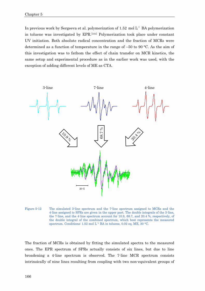
Chapter 5

166

In previous work by Sergeeva et al. polymerization of 1.52 1mol L BA polymerization

in toluene was investigated by EPR.[101] Polymerization took place under constant

UV initiation. Both absolute radical concentration and the fraction of MCRs were

determined as a function of temperature in the range of 50 to 90 °C. As the aim of

this investigation was to fathom the effect of chain transfer on MCR kinetics, the

same setup and experimental procedure as in the earlier work was used, with the

exception of adding different levels of ME as CTA.

20 G

68.7

%

3-line 7-line 4-line

Figure 5-12 The simulated 3-line spectrum and the 7-line spectrum assigned to MCRs and the

4-line assigned to SPRs are given in the upper part. The double integrals of the 3-line,

the 7-line, and the 4-line spectrum account for 10.9, 68.7, and 20.4 %, respectively, of

the double integral of the combined spectrum, which best represents the measured

spectrum. Conditions: 1.52 mol L1 BA in toluene, 0.02 eq. ME, 30 °C.

The fraction of MCRs is obtained by fitting the simulated spectra to the measured

ones. The EPR spectrum of SPRs actually consists of six lines, but due to line

broadening a 4-line spectrum is observed. The 7-line MCR spectrum consists

intrinsically of nine lines resulting from coupling with two non-equivalent groups of

Acrylic Acid

167

two -protons. The 3-line spectrum results from slow rotation of macromolecules, as

discussed in detail in ref.[101]

In Figure 5-12, the three-component fit is shown consisting of the 4-line, 7-line, and

3-line species. All three simulated spectra (top) are combined to best represent the

measured spectrum. The comparison between simulated and measured spectrum

(bottom) demonstrates good accuracy of the simulation. Most of the small deviation

results from the baseline of the experimental spectrum being somewhat tilted. The

ratio of the double integrals yields the ratio of radical concentrations and thus the

fraction of MCRs is given by:

Shown in Figure 5-13 is, to which extent MCRs are observed as a 3-line spectrum

depending on temperature for different CTA concentrations. The 3-line specrum is

associated with a hindered rotation of the macroradical.[101] It is not observed with

model species consisting of a few monomer units only. A reduction of the fraction of

the 3-line spectrum may indicate that chain length is reduced into the oligomeric

region. The 3-line spectrum is observed for polymerizations with 0.02 1mol mol

CTAXXIV to the same extent as without CTA. For 0.05 1mol mol CTA this is

approximately true as well even though the fraction of the 3-line spectrum appears

to some extent reduced. On the other hand, this deviation is within experimental

uncertainty.

Figure 5-14 shows the mole fraction of mid-chain radicals for BA polymerizations

from low temperature, where SPRs predominate, to high temperature, where MCRs

predominate. Depending on temperature, the mole fraction of MCRs is reduced

slightly by CTA. For both 0.02 1mol mol and 0.05

1mol mol the reduction can only

be observed between 0 and 60 °C.

XXIV CTA content is given relative to monomer content.

MCR

3-line 7-line

3-line 7-line 4-linex

(5.24)

Chapter 5

168

-60 -30 0 30 60 900.0

0.2

0.4

0.6

0.8

1.0

/ °C

3

-lin

e /

(3

-lin

e +

7

-lin

e)

Figure 5-13 The share of the 3-line spectrum is given as a function of temperature. Comparing

polymerizations without CTA (squares) taken from ref.[101] to those with addition of

0.02 mol mol1 CTA (circles) the 3-line spectra indicate no effect of CTA. Comparison

with polymerizations, where 0.05 mol mol1 CTA (triangles) have been added, does not

fully support this; there appears to be a slight lowering towards less 3-line signal.

Other than with PLP, continuous initiation ensures that radical concentration is

(pseudo) stationary. Thus, eq. (2.18) can be used to analyze polymerization without

CTA. For polymerizations with CTA, a transfer term, t

tr,CTA CTAk c , has to be added

yielding eq. (5.25). Transfer to monomer may be ignored. Transfer to polymer was

negligible because MCRx did not show any conversion dependence.

Backbiting as well as propagation of MCRs are independent of CTA. There are two

effects of CTA that influence MCRx . First, even small amounts of CTA reduce

MCR bb

MCR t t tt st

SPR MCR p M tr,CTA CTA t MCR t SPR bb2 2

c kx

c c k c k c k c k c k

(5.25)

Acrylic Acid

169

average chain length dramatically, which leads to higher st

tk and tt

tk . At this, the

former coefficient is much higher, and thus crosstermination is the dominant

reaction. Second, a new reaction pathway is opened. MCRs can transfer to the CTA,

which initiates as follow-up reaction, thereby converting MCRs into SPRs.

-60 -30 0 30 60 900.0

0.2

0.4

0.6

0.8

1.0

/ °C

xM

CR

Figure 5-14 The mole fraction of mid-chain radicals during polymerization of BA (1.52 mol L1 in

toluene) under continuous photoinitiation is shown as a function of temperature. The

CTA reduces the fraction of MCRs; this effect increases with the amount of CTA, but

the effect is small and not seen for every temperature. All data points are averages of

multiple measurements. Squares: no CTA, circles: 0.02 mol mol1, triangles:

0.05 mol mol1. Statistical error is calculated as corrected sample standard deviation.

Data of polymerizations without ME is taken from ref.[101]

At lower temperatures, backbiting and crosstermination are controlling for MCRx . As

the activation energy of the former is by 127.1 kJ mol higher, the fraction of MCRs

increases with temperature. The higher rate of termination for polymerizations with

CTA leads to the reduction of MCRs. The difference in MCRx first increases then

decreases again and disappears at ca. 60 °C. At higher temperature, termination

loses importance compared to propagation of MCRs due to its 123.3 kJ mol lower

activation energy.[144,184,185] Moreover, at high temperature crosstermination

Chapter 5

170

additionally loses importance, as there are only few SPRs left for termination with

MCRs.

s

CTAC is approximately unity. In the system BA with thiols s

CTAC is 1.5 and

temperature independent.[180] In general, chain-transfer constants exhibit no or very

low activation energy. That means transfer becomes important when propagation

becomes important. Hence, at high temperature, a reduction of MCRx caused by

increased transfer should be notable. This is not observed; the graphs merge at high

temperature.

This phenomenon needs to be discussed in further detail. The two pathways

reducing MCR concentration by transfer to CTA and by propagation are given by

eq. (5.26) and eq. (5.27), respectively.

In order to estimate whether transfer is significant one has to look at the ratio of the

two reaction rates. Doing so leads to eq. (5.28). With 0.01 1mol mol CTA, the chain-

transfer constant has to be 100 to get a transfer rate as fast as propagation, which

would be an uncommon value. To make transfer the dominant reaction an even

higher value is needed.

Under the assumption that the long-chain approximation holds, eq. (5.29) is used to

calculate the fraction of MCRs for 70 °C, a temperature, which lies in the region

where termination is of less importance. Still, the differences are only a minimum

value (v.i.).

t t t

tr p CTA CTA MCR Rr k C c x c (5.26)

t t

p p M MCR Rr k c x c (5.27)

tttr CTACTAt

Mp

r cC

cr (5.28)

Acrylic Acid

171

The following Arrhenius parameters are used for calculation:[144]

In Table 5-3 the difference between MCRx without transfer to CTA and MCRx with

transfer to CTA is given in percentage points. The log-chain approximation was used

for calculation and, due to shorter chains, termination is higher for polymerization

with CTA further decreasing MCR.x Thus, the differences are only a minimum value.

In the experiment with the higher CTA concentration, a stronger effect is predicted.

As the effect is reduced by conversion, values at zero and 50 % conversion are given. .

Within experimental accuracy, no conversion effect could be observed. Without

transfer, a degree of monomer conversion of 0.9 would result in one percent point

increase of MCR ,x eq. (5.29), which is within error range of MCRx measurement.

At 70 °C, the measured difference of MCRx between polymerization without CTA and

with 0.02 1mol mol CTA is 0.61 percentage points and between polymerization

without CTA and with 0.05 1mol mol CTA is 3.1 percentage points. Adding

experimental error of 2 percentage points, which is more than twice the corrected

sample standard deviation, gives 2.6 and 5.1, respectively. These values are already

very close to 1.87 and 4.53, the calculated differences for t

CTA 10C and below 2.77

and 6.62, the calculated values for t

CTA 15.C Besides, if the latter value of the

constant were right, a notable conversion dependence would apply. Thus, t

CTAC

seems to be below 10 and is certainly below 15.

bb

MCR t t

p M tr,CTA CTA bb

kx

k c k c k

(5.29)

17 1

bb

1t 6 1 1

p

31.7 kJ mol4.47 10 exp s

28.9 kJ mol1.52 10 exp L mol s

kR T

kR T

Chapter 5

172

Table 5-3 The difference between xMCR without transfer to CTA to xMCR with transfer at 70 °C is

given in percentage points. Long-chain approximation is made, thus calculated

numbers are the minimum values. The initial value and the one at 50 % is given,

because the value is a function of conversion (both monomer and CTA)

10.02 mol mol CTA 10.05 mol mol CTA

X

t

CTAC

0 0.5 0 0.5

1 0.19 0.11 0.47 0.27

5 0.94 0.53 2.32 1.31

10 1.87 1.05 4.53 2.59

15 2.77 1.57 6.62 3.83

100 15.72 9.57 31.09 20.76

200 26.74 17.37 46.13 34.03

300 34.88 23.86 54.99 43.25

By calibration with TEMPO, absolute radical concentrations can be obtained from

the double integral of the EPR signal. The overall absolute radical concentrations for

different conditions are given in Figure 5-15. Throughout the polymerization

reaction, high stationary radical concentrations are observed. Addition of CTA

causes a reduction of the radical concentration by about a factor of 3. The reduction

does not increase linearly with CTA content. From 0.02 1mol mol to 0.05

1mol mol

the reduction is only about 30 %.

The difference in radical concentration between the three reaction mixtures may, to

some extent, be explained by the difference in tk resulting from different chain

lengths. GPC analysis of a sample from polymerization without CTA at 20 °C gave

an nM of

4 13.61 10 g mol (Ð = 2.2). Applying the Mayo equation, eq. (2.12), and

assuming s

CTA 1.0,C the addition of 0.02 1mol mol CTA reduces chain length from

282 to 50. With l 0.2 the composite model, eq. (2.34), yields an associated

reduction of tk by a factor of 1.4. According to eq. (2.6) steady-state radical

concentration is proportional to the reciprocal square root of tk . Thus, the reduction

of Rc is by a factor of 1.2. Further reduction of the radical concentration may arise

Acrylic Acid

173

from termination by CTA radicals. For polymerizations with a smaller rate of

initiation and therefore a lower rate of termination leading to longer chains the

impact of a CTA would be stronger. It would be interesting to do the same

experiment with low radical concentration 8 1(10 mol L ) , but these conditions are at

present beyond EPR measuring range.

-60 -30 0 30 60 900

2

4

6

/ °C

c R /

106 m

ol

L

1

Figure 5-15 Overall radical concentrations (SPRs and MCRs) of polymerizations with different

concentrations of CTA are shown as a function of temperature. Black squares: no CTA,

red circles: 0.02 mol mol1, blue triangles: 0.05 mol mol1. Data of polymerizations

without ME is taken from ref.[101]

The radical concentrations in the three reaction mixtures exhibit exactly the same

temperature dependency. The radical concentration slightly increases with higher

temperature. Then it increases from 0 to 30 °C, and afterwards decreases again, but

slowly or stays constant.

The rate of initiation is the same, because in case of photoinitiation the energy for

decomposition of initiator is not supplied thermally. Termination increases with

temperature, but only slightly, as the activation energy of tk is as low as

Chapter 5

174

15.6 kJ mol . [144,184,185] Hence, with a constant fraction of MCRs a slight decrease of

the radical concentration with higher temperature would be expected, but this is not

the case. In the temperature region under investigation a dramatic shift in MCRx

takes place. Due to MCRs terminating more slowly, a higher fraction of MCRs allows

for a higher radical concentration. The fact that the inflection points of the curves in

Figure 5-14 and Figure 5-15 are at the same temperature also supports MCRs

kinetics as being the reason.

-60 -30 0 30 60 900.4

0.6

0.8

1.0

1.2

1.4

/ °C

c R /

cR(2

0 °

C)

0.0

0.2

0.4

0.6

0.8

1.0

xM

CR

Figure 5-16 Overall stationary radical concentration (SPRs and MCRs) is plotted in olive as a

function of temperature scaled to the radical concentration at 20 °C. For comparison

the fraction of midchain radicals is plotted in pink. (upper half filled squares: no CTA,

right half filled circles: 0.02 mol mol1, lower half filled triangles: 0.05 mol mol1)

In order to better visualize both the relationship between radical concentrations

during polymerization with different CTA content and how they are related to the

fraction of MCRs, both quantities are plotted together in Figure 5-16. At this, radical

concentration is scaled to the value at 20 °C which is near the inflection point. The

radical concentration curves of the three reaction mixtures are on top of each other

Acrylic Acid

175

and they are also (though somewhat more scattered) on top of the curves fir the MCR

fraction.

The fact, that the three curves have, within experimental error, the same shape even

though chain length of both MCRs and SPRs are quite different points towards

MCRs and SPRs showing the same chain-length dependency of tk .

In this subchapter it has been shown that the chain-transfer constant of MCRs

cannot be significantly higher than the chain-transfer constant of SPRs.

Even without considering higher termination rate for polymerizations with CTA, s

CTAC still cannot be above 15, which would be too low to make transfer of MCRs a

major reaction pathway. Thus, effects so far attributed to high transfer of MCRs to

CTA have to be explained differently, e.g., a reduction of -scission products may be

the result of increased termination. Moreover, an enhancement of rate of

polymerization may result from additional initiation by the thiol-ene reaction.

Furthermore, it was demonstrated how termination increases and overall radical

concentration drops by a factor of three upon addition of 0.02 1mol mol CTA.

However, the reduction of the fractions of MCRs by higher crosstermination is only

small.

5.1.6 CCTAs of ME with AA

The chain-transfer constant of SPRs to ME during polymerization of AA was

determined by the Mayo plot, which has been developed for systems with only one

growing radical species. In the following, it will be shown that the Mayo procedure

can be used for this system with MCRs being present to determine s

CTA .C This is

related to a detailed analysis of MCR kinetics by Nikitin et al.[38]

The basic idea of the Mayo equation is that the average chain length is determined

by the ratio of growth of chains to the rates of termination and transfer, eq. (5.30).

p

t tr

n

ri

r r

(5.30)

Chapter 5

176

The two stopping events of the chain growth can be separated, eq. (5.58)

In case of SPR-MCR kinetics, the first term of eq. (5.31) RHS need not be considered

further, but the second has to be. Transfer to growth of both radical species may be

expressed by eq. (5.32).

A simplified treatment of the denominator of eq. (5.32) RHS has already been

discussed in subchapter 2.3.3 (see eq. (2.17)). The same treatment can be made for

the numerator, but only under the condition: s t

tr,CTA SPR tr,CTA MCRk x k x . In

subchapter 5.1.5, it has been shown that the chain transfer constant of MCRs does

not exceed the corresponding one for SPRs. Thus, s

tr,CTAk is a much larger than t

tr,CTAk and eq. (5.33) can be used for good approximation. For systems, in which

eq. (5.33) is valid, the Mayo plot yields s

CTA .C

The Mayo plot for the product of the polymerization of 0.10 g g1 AA at 50 °C in

aqueous solution with 6.56 mmol L1 of photoinitiator D1173 is given in Figure 5-17.

1 t tr

p p

n

r ri

r r

(5.31)

s t

tr,CTA CTA SPR tr,CTA CTA MCRtr R R

s t

p p M SPR p M MCRR R

s t

CTA tr,CTA SPR tr,CTA MCR

s t

M p SPR p MCR

k c c x k c c xr

r k c c x k c c x

c k x k x

c k x k x

(5.32)

s

CTA tr,CTAtr

s

p M p

c kr

r c k

(5.33)

Acrylic Acid

177

The data points were deduced from wM via eq. (4.2), because this was found to give

better results for the MAA/ME system (see subchapter 4.1.1).

The best fits to a straight line according to eq. (2.12) yields:

The value of s

CTAC of AA and ME in aqueous solution is higher than

CTA 0.12 0.01C the value for MAA and ME in aqueous solution, which may be

explained by the stability of MAA macroradicals being higher than the stability of

AA macroradicals (compare subchapter 2.2.1).

0.000 0.005 0.010 0.0150.000

0.002

0.004



n

cME

/ cAA

Figure 5-17 The Mayo plot, eq. (2.12), of the polymeric product of the polymerization of 0.10 g g1

AA at 50 °C in aqueous solution with 6.56 mmol L1 of photoinitiator D1173 to low

conversion. Data points (blue circles) were deduced from MW via eq. (5.25). The

corresponding best fits to a straight line is given in red.

s

CTA 0.28 0.04C (5.34)

Chapter 5

178

5.1.7 Determination of kp for AA Macromonomers by 1H-NMR

Above 90 °C, macromonomers, MM, are formed during AA polymerization by

backbiting and subsequent -scission to a significant extent. They can propagate,

which leads to the formation of MCRs, which may undergo -scission again forming

MMs (see subchapter 2.3.1). Hence, the separation of the corresponding coefficients

is difficult. The problem was circumvented by synthesizing MM at high temperature

(subchapter 3.14.3) and observing their propagation at lower temperature so that -

scission (and thus formation of MM) as follow-up reaction can be excluded.

Figure 5-18 1H-NMR spectrum ( 300 MHz) of AA macromonomers, MM(AA), synthesized in DMSO

at 138 °C. The positions of the protons are attributed to the signals via blue arrows.

The MM lines are: 1H-NMR (D2O): = 1.73 (bs, 2H), 2.36 (bs, H), 5.69 (bs, H), 6.18 (bs,

H). The prediction of the shift by ChemDrawTM is 1.75, 2.35, 5.95, and 6.54,

respectively.

In Figure 5-18, the 1H-NMR spectrum of MM(AA) synthesized in DMSO at 138 °C is

given. The positions of the protons are attributed to the signals via arrows. The

chemical shift of the two protons of the terminal double bond 5.69 (bs, 1H) and 6.18

(bs, 1H) cannot be assigned to product from disproportionation, as the shift of such

Acrylic Acid

179

protons would be different. Moreover, vicinal coupling is typically very small, while

geminal trans-coupling is always observed in high-resolution 1H-NMR spectroscopy

Figure 5-19 shows the ESI-MS spectrum of the sample, of which the 1H-NMR is

depicted in Figure 5-18. The signals marked by their m / z values are multiples of AA

monomer mass. The corresponding Lewis structure of the MM(AA) is given as well.

The molecule with 935.3 u consists of eleven monomer units, thus mostly oligomeric

MMs have been produced. Furthermore, no disproportionation patterns (two lines of

equal height with the difference of 2.02 u) were found in the mass spectrum giving

additional support for synthesis of MMs.

Figure 5-19 ESI-MS spectrum (negatively charged ions; methanol and water) of MM(AA)

synthesized in DMSO at 138 °C. The signals marked are multiples of AA monomer

mass. The structure of the MM(AA) is given as well. The molecule with 935.3 u

consists of eleven monomer units. The smaller signals in between are mostly from

multible-charged polymer.

In Figure 5-20, the polymerization of MM(AA) synthesised in o-xylene with AA in

aqueous solution is depicted. The polymerization was carried out in NMR tubes.

Both the degree of AA conversion and the ratio of MM(AA) to AA was measured via 1H-NMR . The polymer signal is small at low conversion and in broad. Calculating X

Chapter 5

180

from the ratio of monomer and polymer signal would be rather imprecise, even more

so, as the MM already gives a polymer signal (compare Figure 5-18). By use of the

aromatic signal of residual o-xylene as reference the measurement becomes more

accurate.

0 2000 4000 6000 80000.00

0.25

0.50

0.75

X

time / s

0.00

0.25

0.50

0.75

c MM

/ c

M

Figure 5-20 MM(AA) and AA were polymerized in NMR tubes. The degree of AA conversion was

measured by 1H-NMR (squares), as was the ratio of MM(AA) to AA (stars).

Consumption of monomer and macromonomer is the same, as the ratio stays constant

towards higher conversion of AA. The dotted line indicates the initial ratio. The

synthesis of MMs had been carried out in o-xylene and the aromatic signal of residual

o-xylene was used as reference. cAA = 0.047 mol L1, cMM(AA) = 0.021 mol L1 (first

moment), cV-50 = 0.037 mol L1, in aqueous solution at 50 °C.

Because of steric hindrance, propagation of MCRs with MMs was assumed

negligible. Different initial ratios around 1:1 were polymerized to observe both AA

and MM(AA) with similar accuracy. The coefficient of propagation of an SPR with an

MM, s

p,MMk , was estimated via PREDICITM simulation of profiles the X and the

MM M/c c profiles as a function of time. The result is given by eq. (5.35). Considering

the higher stability of the tertiary radical, it appears reasonable that the addition of

an MM to an SPR is favored.

Acrylic Acid

181

In case that MCRs also add MMs, the reactivity ratios should be unity as MM M/c c is

independent of X.

5.1.8 Modeling Polymerization at 35 to 80 °C

The previous subchapters describe the kinetic information available from

independent experiments taken either from literature or from this study. The basis

for modeling polymerization of AA between 35 °C and 90 °C were mostly conversion

vs. time profile.XXV Furthermore, MMDsXXVI of polymerizations between 35 °C and

65 °C were used.

t

pk was scaled to s

pk and estimated for each conversion vs. time profile of

polymerizations without addition of CTA. The corresponding Arrhenius plot is shown

in Figure 5-21. Data from polymerizations with V-50 being the initiator are in good

agreement with those from polymerizations with VA-086 being the initiator. The

concatenate, best fit to a straight line yields eq. (5.36)

According to eq. (5.36) the difference in activation energy between t

pk and s

pk is

t s 1

A p A p 19.2 kJ molE k E k , which is in good agreement with 120.5 kJ mol

calculated from ref. values[36,37] and higher than t s 1

A p A p 11.2 kJ molE k E k

reported for BA.[42]

XXV Some of the conversion time data used for modeling in this subchapter were taken from

previous work.[147] Moreover, three conversion vs. time profiles were a courtesy of Patrick

Drawe. XXVI The Lacík group (Polymer Institute SAV, Slovakia) did the SEC analysis.

s s

p,MM p1.4 0.2k k (5.35)

t s

p p

2314/ 2.41 exp

/ Kk k

T

(5.36)

Chapter 5

182

0.0028 0.0030 0.0032

-6.5

-6.0

-5.5

-5.0

-4.5

35 °C

90 °C

ln (

kt p /

ks p )

T 1

/ K 1

Figure 5-21 Arrhenius plot of the ratio of kpt to kp

s. The values were estimated from conversion vs.

time profiles by PREDICITM. Red circles: V-50 was used as initiator; blue triangles:

VA-086 was used as initiator. The concatenate, best fit to a straight line is given in

purple. The so-obtained difference in EA of kpt and kp

s is in agreement with

literature.[36,37]

MMDs have been measured for different temperatures (35, 50, and 65 °C) and for

different levels of initiator concentration (0.01, 0.001, and 10.0001 g g). With

5

tr,M 5.37 10C taken from ref.[90] MMDs were predicted too high. The deviation was


concentration and low temperature. Therefore, transfer to monomer had to be

increased and 4

tr,M 1 10C yields simulated MMDs being in satisfying agreement

experimental ones.

10.1 g g AA in water were polymerized at 35, 50, and 65 °C up to complete

conversion with V-50 as initiator at levels of 210 , 310 , and 4 110 g g . Molar mass

was found to vary only slightly with initiator concentration. Without considering

transfer to monomer MMDs were predicted too high. The deviation was


concentration and low temperature. In order to illustrate the influence of tr,M ,C two

Acrylic Acid

183

measured MMDs are plotted together with the corresponding simulation not

featuring transfer to monomer in Figure 5-22. At relatively high rate of initiation

(left) the deviation between experiment and simulation is rather weak, but at low

rate of initiation the deviation is strong. Therefore, simulation of MMDs required s

tr,MC being:

4 5 6 7

w (

lg (

M /

g m

ol

1))

lg ( M / g mol1

)

left:

102

g g1

65 °C

right:

103

g g1

50 °C

CM

= 0

Figure 5-22 Comparison of measured and simulated MMDs without considering transfer to

monomer shows deviation, which is was systematically higher towards lower rate of

initiation. Blue line: polymerization of 0.1 g g AA to full conversion (initiator

concentrations and temperatures given for each graph). Very high molar masses were

reached and a significant amount of polymer was outside of SEC calibration. This

resulted in a kink as calibration artifact. Red line: simulation.

In Figure 5-23, measured MMDs are compared to predictions by the PREDICITM

model. The measured MMDs feature a kink slightly above 6 110 g mol . This is a

calibration artifact due to end of direct calibration at this point as for MMDs from

MAA polymerization (subchapter 4.2.2). With transfer to monomer being included,

measured and predicted MMDs agree within experimental uncertainty, which is

s

tr,Ms 5

tr,M s

p

7.5 10k

Ck

(5.37)

Chapter 5

184

higher in this case due to said problem of MMDs being partly out of calibration

range. MMDs of polymerizations with CTA are not shown as their prediction is

rather trivial, provided that pk and tr,CTAC are known with high accuracy.

For polymerizations with higher monomer content, only a few conversion vs. time

profiles were measured. Eq. (5.14) leads to acceptable representation of measured

data, but especially for 10.3 g g AA a clear deviation in shape is seen. Probably an

equation of the form eq. (4.11) (see subchapter 4.2.1) would lead to better results. For

an evaluation like this, more data would be needed.

In Figure 5-24, the comparison of measured and simulated AA conversion vs. time

plots of polymerization of 10.1 g g AA at temperatures from 35 to 80 °C

demonstrates the quality of the model in this temperature range.

The agreement of measured and simulated AA conversion vs. time plots of 10.1 g g

AA polymerization at temperatures from 65 to 80 °C upon addition of CTA from

small to very high amounts can be observed in Figure 5-24 and Figure 5-25. The

quality of the prediction does not reach the level as obtained for polymerization

without CTA, but is still satisfactory, especially when one considers the lower

experimental reproducibility of experiments involving CTA. The conversion vs. time

profiles of polymerizations with highest ME content show good agreement with the

simulation (Figure 5-25). For some other polymerizations with very high ME content

(not shown here) a drift towards higher rate of polymerization was found, i.e. at high

CTA content further increase of CTA level did not lead to further decrease of

polymerization rate but to a slight increase again. This effect might originate from

additional initiation by the thiol-ene reaction, the rate of which could not be

quantified. It may not be explained by high transfer of MCRs to CTA, because for the

model system BA/ME it was found that t

CTAC cannot be much higher than s

CTAC (see

subchapter 5.1.5).

The parameters of the model for the polymerization of non-ionized AA are

summarized in Table 5-2.

4 5 6 7 4 5 6 7

102

g g1

65 °C

102

g g1

50 °C

102

g g1

35 °C

103

g g1

65 °C

103

g g1

50 °C

103

g g1

35 °C

104

g g1

65 °C

104

g g1

50 °C

Figure 5-23 Comparison of measured and simulated MMDs. Blue line: polymerization of 0.1 g g AA to full conversion (initiator concentrations and temperatures

given for each graph). Very high molar masses were reached and a significant amount of polymer was outside of SEC calibration. This resulted in a

kink as calibration artifact. Red line: simulation.

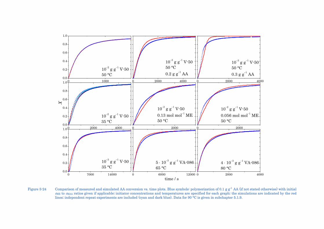
0 10000.0

0.2

0.4

0.6

0.8

1.0

0 2000 4000 0 2000 4000

0 2000 40000.0

0.2

0.4

0.6

0.8

1.0

0 2000 0 2000

0 7000 140000.0

0.2

0.4

0.6

0.8

1.0

0 6000 12000 0 2000 4000

102

g g1

V-50

50 °C

103

g g1

V-50

50 °C

0.2 g g1

AA

103

g g1

V-50

50 °C

0.3 g g1

AA

time / s

X

102

g g1

V-50

35 °C

102

g g1

V-50

0.13 mol mol1

ME

50 °C

102

g g1

V-50

0.056 mol mol1

ME

50 °C

103

g g1

V-50

35 °C

5 103

g g1

VA-086

65 °C

4 103

g g1

VA-086

80 °C

Figure 5-24 Comparison of measured and simulated AA conversion vs. time plots. Blue symbols: polymerization of 0.1 g g AA (if not stated otherwise) with initial

cME to cMAA ratios given if applicable; initiator concentrations and temperatures are specified for each graph; the simulations are indicated by the red

lines; independent repeat experiments are included (cyan and dark blue). Data for 90 °C is given in subchapter 5.1.9.

0 8000 160000.0

0.2

0.4

0.6

0.8

1.0

0 6000 12000 0 9000 18000

0 10000 200000.0

0.2

0.4

0.6

0.8

1.0

0 2000 4000 0 2000 4000

0 1000 2000 3000 4000 50000.0

0.2

0.4

0.6

0.8

1.0

0 3000 6000 0 4000 8000

0.88 cmol mol1

ME

80 °C

22 cmol mol1

ME

65 °C

14 cmol mol1

ME

65 °C

time / s

X

22 cmol mol1

ME

80 °C

14 cmol mol1

ME

80 °C

5.7 cmol mol1

ME

80 °C

2.6 cmol mol1

ME

80 °C

2.6 cmol mol1

ME

65 °C

0.88 cmol mol1

ME

65 °C

Figure 5-25 Comparison of measured and simulated AA conversion vs. time plots. Blue symbols: polymerization of 0.1 g g AA with 0.005 g g and 0.004 g g

VA-086 as the initiator at 65 °C and 80 °C, respectively. The particular initial cME to cMAA ratios given for each graph. The simulations are indicated

by the red lines; independent repeat experiments are included (cyan).

Chapter 5

188

5.1.9 Modeling Polymerization at High Temperature

For polymerizations at high temperature, which means for this system above 90 °C,

additional reactions have to be considered leading to an even more complex reaction

scheme. -scission of MCRs may take place building macromonomers. These

propagate to form lMCR s, which may add monomer and thus grow further or

undergo -scission again. The corresponding scheme is shown in Table 5-4 top.

The implementation of the additional high-temperature reactions into PREDICITM can

be simplified. Nikitin et al.[42] modeled BA polymerization up to 170 °C with a

reduced number of reactions. They condensed the reaction scheme in Table 5-4 top

into the reaction scheme in Table 5-4 bottom introducing the compounded rate

coefficients defined by eq.(5.38) and eq. (5.39). This strategy was adopted for the

present modeling work.

Table 5-4 The additional reactions that have to be taken into account for high temperature

polymerization are shown in the upper part. For modeling of BA polymerization up to

170 °C as has been shown by Nikitin et al.[42] a simplified approach is possible to

account for -scission of MCRl, MM propagation, and MCRl propagation. The

corresponding scheme is shown in the lower part.

Additional high temperature reactions

-scission of

sMCR s SPR, 2 2 SPR,3 3MCR ,

R R MM R MMi ii

k

lMCR l SPR, SPR,jMCR ,

R R MM R MMi j ii j

k

SPR propagating with of MM l

sp,MM

SPR, MCR ,R MM Ri j i j

k

propagation of lMCR

l

tp

SPR, 1MCR ,R M R i ji j

k

s

p,MM

1 t

p M2

kk k

k k c

(5.38)

s

p,MMt

2 p M t

p M2

kk k c

k k c

(5.39)

Acrylic Acid

189

Simplified Treatment

1SPR, SPR,R MM R MMi j j i

k

2SPR, SPR,R MM Ri j i j

k

For modeling polymerization at intermediate temperature up to 90 °C, t

pk was

scaled to s

pk with the ratio being temperature dependent (see subchapter 5.1.8).

Extrapolation of this ratio up to 170 °C gave reasonable results, as will be shown

below. Determining the influence of t

pk and k on rate of polymerization, molar

mass, and branching is not trivial. Their respective influence also depends on other

parameters. Higher t

pk leads to higher polymerization rate, but has no direct

influence on branching level. k also increases polymerization rate, especially if t

pk

is relatively low and bbk high. k reduces branching, especially if t

pk is low in

comparison. However, the effect of t

pk and k on molar masses is reverse. The final

coefficients were obtained by keeping the Arrhenius expression for t

pk derived from

moderate temperature polymerizations and adjusting k for best representation of

measured conversion vs. time profiles and molar masses. The resulting Arrhenius

plot is given by eq. (5.36).

The corresponding activation energy is 1127 kJ mol , which is close to the activation

energy of 1125 kJ mol found for k during thermal degradation of polyethylene.[186]

The activation energy is significantly higher than 163.9 kJ mol , the activation

energy found for the -scission of BA.[42] The absolute value of k in the considered

temperature range is also bigger than the value found for BA. These comparisons

suggest that this value of k might be too high.

In order to obtain better representation of experimental data (conversion vs. time

profiles, molar masses, branching level) by simulations of the model, the parameters

t s

p p/k k and 1,1,tt 1,1,ss

t t/k k as well as composite model parameters of MCRs have been

widely varied. MCRs kinetics do not have a large impact on the simulation. A slight

41 18 1.5 10

/ s 1.9 10 exp/ K

kT

(5.40)

Chapter 5

190

variation of bbk has been attempted, but as the prediction of the branching level is

in good agreement with measured data, this coefficient appears to be accurate.

The 1,1,ss

tk value measured for AA[36] appears rather high in comparison to other

monomers, which suggests that a lower value might lead to better modeling results.

Nevertheless, lowering 1,1,ss

tk by a factor of three the virtual dependence of t s

p p/k k on

initiator content at 90 °C remains (see Figure 5-21). Higher and lower values for this

coefficient (by a factor of 10) were attempted, but the accuracy of the simulation

could not be improved.

Different values for k and t s

p p/k k led to a better representation of conversion vs.

time profiles, but to a prediction of higher molar masses than have been measured,

which is discussed further below.

In Figure 5-26 top, the concentration of branching points, BP ,c is depicted as a

function of conversion and temperature. BPc increases towards higher temperature

and towards higher conversion. The branching level can be predicted very well by

the model over the entire range of temperature and conversion.

In Figure 5-26 bottom, the fraction of short-chain branching is plotted as a function

of conversion and temperature. The simulated values of SCBx decrease towards

higher temperature and towards higher conversion. The experimental values are

much lower than simulated ones. This may be explained by further backbiting of

MCRs moving the radical function backwards along the polymer chain (see

subchapter 2.3.3), a reaction that is not yet included in the model. It should be noted

that long-chain branching does only mean that the branch is at least one monomer

unit longer than a short-chain branch of two monomer units.

Measured and simulated molar mass are compared in Figure 5-27 (top: nM ; bottom:

wM ). While nM decreases notably at high conversion, wM stays relatively constant.

Molar mass decreases towards higher temperature, which is mostly the consequence

of initiator decay being more rapid. The experimental results for molar mass are

somewhat scattered. The model can predict them over the whole range of

temperature and conversion very well.

The conversion vs. time profiles of polymerizations between 90 and 170 °C and the

according simulations are shown in Figure 5-28. Experimental results are from two

different modes of operation of the tubular reactor setup (see subchapter 3.13). The

results from the stopped flow experiments, in which the tubular reactor is bypassed

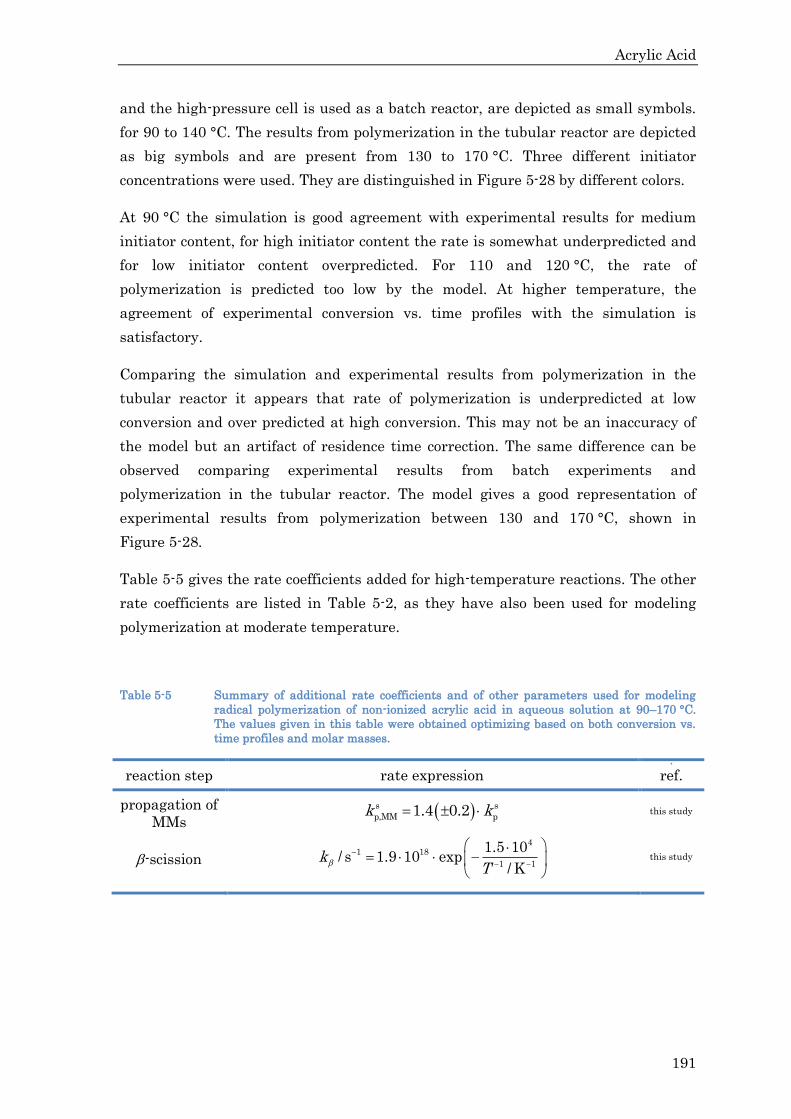
Acrylic Acid

191

and the high-pressure cell is used as a batch reactor, are depicted as small symbols.

for 90 to 140 °C. The results from polymerization in the tubular reactor are depicted

as big symbols and are present from 130 to 170 °C. Three different initiator

concentrations were used. They are distinguished in Figure 5-28 by different colors.

At 90 °C the simulation is good agreement with experimental results for medium

initiator content, for high initiator content the rate is somewhat underpredicted and

for low initiator content overpredicted. For 110 and 120 °C, the rate of

polymerization is predicted too low by the model. At higher temperature, the

agreement of experimental conversion vs. time profiles with the simulation is

satisfactory.

Comparing the simulation and experimental results from polymerization in the

tubular reactor it appears that rate of polymerization is underpredicted at low

conversion and over predicted at high conversion. This may not be an inaccuracy of

the model but an artifact of residence time correction. The same difference can be

observed comparing experimental results from batch experiments and

polymerization in the tubular reactor. The model gives a good representation of

experimental results from polymerization between 130 and 170 °C, shown in

Figure 5-28.

Table 5-5 gives the rate coefficients added for high-temperature reactions. The other

rate coefficients are listed in Table 5-2, as they have also been used for modeling

polymerization at moderate temperature.

Table 5-5 Summary of additional rate coefficients and of other parameters used for modeling

radical polymerization of non-ionized acrylic acid in aqueous solution at 90–170 °C.

The values given in this table were obtained optimizing based on both conversion vs.

time profiles and molar masses.

reaction step

rate expression +

ref.

propagation of

MMs

s s

p,MM p1.4 0.2k k this study

-scission

41 18

1 1

1.5 10/ s 1.9 10 exp

/ Kk

T

this study

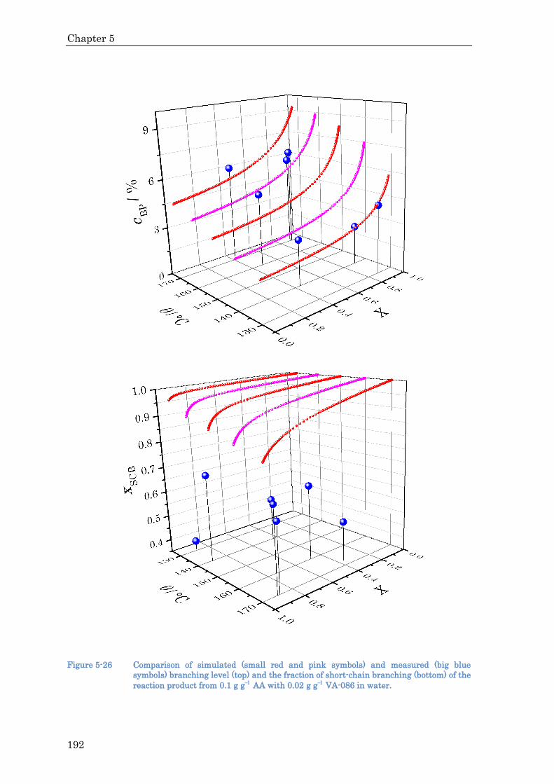
Chapter 5

192

Figure 5-26 Comparison of simulated (small red and pink symbols) and measured (big blue

symbols) branching level (top) and the fraction of short-chain branching (bottom) of the

reaction product from 0.1 g g AA with 0.02 g g VA-086 in water.

Acrylic Acid

193

Figure 5-27 Comparison of simulated (small red and pink symbols) and measured (big blue

symbols) molar mass of the reaction product from 0.1 g g AA with 0.02 g g VA-086

in water.

0 2000 40000.0

0.2

0.4

0.6

0.8

1.0

0 1000 2000 0 300 600

0 200 4000.0

0.2

0.4

0.6

0.8

1.0

0 100 200 0 50 100

0 40 800.0

0.2

0.4

0.6

0.8

1.0

0 30 60 0 30 60

100 °C90 °C

160 °C 170 °C150 °C

140 °C130 °C120 °C

110 °C

X

time / s

Figure 5-28 Comparison of measured (symbols) and simulated (line) conversion vs. time plots of the polymerization of 0.1 g g AA with 0.01 g g VA-086 (red

circles), 0.005 g g VA-086 (green triangles), 0.002 g g VA-086 (blue and cyan squares). The mode of operation was either stopped flow (batch

experiment) given by small symbols or polymerization in the tubular reactor depicted as big symbols.

Acrylic Acid

195

Alternative values for kpt and k

The unexpected high value for k and the rather low quality of polymer samples

from high-temperature experiments subjected to molecular mass analysis led to the

idea that molar mass may be ignored and instead conversion vs. time profiles may

have priority for optimization of the model. This led a similar k value as found for

of BA and t s

p p/k k became even more similar to the value reported for BA than with

the approach including optimization with respect to molar masses.

The corresponding activation energy is 165 kJ mol , which is close to the activation

energy of 163.9 kJ mol found for the -scission of BA.[42] The Arrhenius pre-

exponential factor is slightly lower than 1.5 found for the -scission of BA.[42]

The corresponding difference in activation energy between t

pk and s

pk is

t s 1

A p A p 11.5 kJ molE k E k , which is lower than 120.5 kJ mol calculated from

ref. values,[36,37] but surprisingly similar to t s 1

A p A p 11.2 kJ molE k E k reported

for BA.[42]

The agreement between simulations and experimental conversion vs. time profiles

still varies with initiator concentration, but the underprediction of polymerization

rate at 110 and 120 °C is much weaker for this approach and in general the

representation of experimental conversion vs. time profiles is better.

The alternative t s

p p/k k expression, eq. (5.42), was not developed for simulation of AA

polymerization between 35 to 80 °C.

31 9 7.8 10

/ s 1.3 10 exp/ K

kT

(5.41)

t s

p p

1382/ 0.38 exp

/ Kk k

T

(5.42)

0 2000 40000.0

0.2

0.4

0.6

0.8

1.0

0 1000 2000 0 300 600

0 200 4000.0

0.2

0.4

0.6

0.8

1.0

0 100 200 0 50 100

0 40 800.0

0.2

0.4

0.6

0.8

1.0

0 30 60 0 30 60

100 °C90 °C

160 °C 170 °C150 °C

140 °C130 °C120 °C

110 °C

X

time / s

Figure 5-29 Comparison of measured (symbols) and simulated (line) conversion vs. time plots of the polymerization of 0.1 g g AA with 0.01 g g VA-086 (red

circles), 0.005 g g VA-086 (green triangles), 0.002 g g VA-086 (blue and cyan squares). The simulations show here were done with different values

forkpt and k than in Figure 5-28.

Acrylic Acid

197

Table 5-6 gives alternative values for the rate coefficients added for high-

temperature reactions. The other rate coefficients are listed in Table 5-2, as they

have also been used for modeling polymerization at moderate temperature.

Table 5-6 Summary of alternative rate coefficients, which were obtained by optimization based

on conversion vs. time profiles only, ignoring molar masses.

reaction step

rate expression

ref.

propagation of

MCRs

t s

p p

1382/ 0.38 exp

/ Kk k

T

this study

-scission

31 9 7.8 10

/ s 1.3 10 exp/ K

kT

this study

5.2 Model Development for Ionized Acrylic Acid

Ionization of monomer and polymer alters rate coefficients. For polymerization of

fully ionized monomer, reactions between ionized and non-ionized species need not

be considered, but even in this case the level of complexity rises in comparison to

polymerization of non-ionized monomer, as rate coefficients of ionized species depend

on ionic strength. The effect of ionic strength on, e.g., s

pk is considerable, as will be

shown in subchapter 5.2.1

For polymerization of partly ionized monomer complexity is further increased,

because reactions of ionized with non-ionized species have to be considered and as

the ApK values of monomer and polymer differ (see subchapter 5.2.10), the degree of

ionization of both monomer and polymer changes with conversion.

The kinetic scheme for the polymerization of ionized AA is principally the same as

for non-ionized AA, as no additional reactions occur. Thus, the kinetic scheme used

for modeling consists of the kinetic scheme given in the upper part of Table 5-1 and

includes kinetics of MCRs (Table 5-1 middle). High-temperature reactions of ionized

AA have not been modeled. The set of rate coefficients and other variables, e.g.,

density, was taken from modeling of the non-ionized monomer (Table 5-2) and

extended as is summarized in Table 5-7 for fully ionized AA and summarized in

Table 5-8 for partly ionized AA at the end of this section.

Chapter 5

198

Some kinetic information on the effects of ionization is known from literature, but

most dependencies have not yet been studied in detail. For modeling, a combination

of re-evaluation of data reported by other groups and new experimentsXXVII were

analyzed. The level of complexity for modeling the polymerization non-ionized AA

(see subchapter 5.1) already being higher than for MAA (see chapter 4) is further

increased in this system. As modeling of the polymerization of fully ionized AA is

easier, first a summary of the rate coefficients for this system is given with the

corresponding modeling work following in subchapter 5.2.5. Afterwards the aspects

of the partly ionized systems are discussed and predictions of the so-assembled

model are shown in subchapter 5.2.11.

5.2.1 kp of Fully Ionized AA and dependence on Ionic Strength

s

pk of fully ionized AA has been measured via PLP–SEC only for one concentration 1(0.05 g g at 6 °C).[76] However, the dependence of s

pk of fully ionized AA on monomer

content should be similar to the dependence of pk of fully ionized MAA on monomer

content.[11] pk of fully ionized MAA is overall less dependent on monomer content

than the pk of non-ionized MAA and towards dilute solution a decrease of

pk

instead of an increase as for the non-ionized monomer was found.[11] The dependence

of s

pk of AA on AAw and is discussed in subchapter 5.2.6. The result with respect

to AAw at full ionization is given by eq. (5.43).

There is no value available for t

pk of partly ionized AA and only one value for t

pk of

fully ionized AA, which was obtained by parameter estimation from SP–PLP–EPR

radical concentration vs. time profiles.[77] The literature value was estimated under

the assumption that MCRs do not terminate, whereas in the present study the

termination of MCRs is taken into account.

XXVII Patrick Drawe carried out the experiments with V-50 as initiator and fully ionized AA.

s 1 1 7

p

1395/ L mol s 1.94 10 exp

/ K

0.16 1 0.16 exp 3.7 1.6 0.04

kT

w w

(5.43)

Acrylic Acid

199

It appears reasonable that t

pk is influenced by ionization in the same way as s

p .k

The same assumption has been made for the dependence of t

pk on AA content and

gave good results (see subchapter 5.1). As a consequence, t

pk is higher than the

value estimated upon neglect of MCR termination.[77] The approach used for this

modeling work leads to good representation of experimental data (v.i), whereas the

lower value from ref.[77] leads to underprediction of the rate of polymerization.

Figure 5-30 Rate of polymerization of 0.05 g g1 AA ( = 1) with 12 mmol L1 V-50 as the initiator

in water with different amounts of added NaCl at 50 °C and ambient pressure. The

rate of polymerization augments linearly with amount of added salt. Repeat

experiments show good agreement. This graph is a courtesy from Patrick Drawe.

Eq. (5.38) describes s

pk as a function of monomer content, temperature and degree of

ionization, but does not consider the effect of ionic strength on polymerization

kinetics. The rate of polymerization of 0.05 g g1 AA ( = 1) with 12 mmol L1 V-50 as

the initiator in aqueous solution at 50 °C is shown in Figure 5-30 for different

amounts of added NaCl. The rate of polymerization augments linearly with the

added amount of salt. This increase should be associated with an increase of pk ,

Chapter 5

200

since variation of all other rate coefficients should result in a decrease of

polymerization rate at higher I, as will be discussed below. Kabanov et al.[12]

proposed an ion-pair mechanism as the cause for a higher pk towards increase of I.

Their idea was that the carboxylate unit at the chain-end of the macroradical

interacts with a cation, e.g., Na , which in turn interacts with the carboxylate

moiety of a monomer molecule thus “handing it over” to the radical center and thus

increases rate of propagation. These authors did not consider MCRs, as backbiting

was not known for AA polymerization at the time of publication. The dependence of

s

pk on both monomer content and degree of ionization can be explained via the

transition state structure. The trends found experimentally are reproduced by

calculation.[169] So far, no attempts have been made to calculate s

pk for ionized acrylic

acid based on transition state theory with different amounts of cations being present

around the radical center.

If an ion-pair mechanism increases the rate of propagation, this effect should be

stronger for MCRs – approximately twice as large – because they have carboxylate

groups on both sides “handing over” monomer. Thus, the rate enhancing effect by

addition of counter ions should be stronger for conditions favoring MCRs, e.g., low

monomer concentration. Moreover, the rate enhancement by additional counterions

should be stronger for NaA than for NaMA. Indeed, overtitration with sodium

hydroxide, which increases the number of counter ions, results in a stronger rate

enhancement of polymerization of NaA than of NaMA.[12] The enhancing effect being

weaker for NaMA may also explain, why it was not found in PLP-SEC experiments

of NaMA (see subchapter 2.4.3).

By close inspection of the profiles given in Figure 5-30, it can be seen that the

maximum of rate of polymerization slightly shifts to higher degrees of monomer

conversion towards higher salt concentration. This observation supports the idea of a

stronger impact on MCRs, because their fraction increases towards higher X.

However, the variation of MCRx is weak and more experiments under conditions,

which favor MCRs to different extent, should be carried out.

As the addition of salt should have an influence on all coefficients probably with

exception of initiator decay, an attempt was made to still find a good description for

the influence of added salt based on data given. Additional counterions should

increase the termination and backbiting rate, and thus decrease the rate of

polymerization. However, as an enormous augmentation of the rate of

polymerization was found, the amplifying effect on propagation seems to be

dominant. For modeling purpose, the effect of higher I on pk was assumed to apply

twice as strong for t

pk . Consequently, s

pk is multiplied with the factor of

Acrylic Acid

201

enhancement of propagation, I , and t

pk scaled to the already enhanced s

pk is also

multiplied with I , viz., the propagation of MCRs is augmented by 2.I

I was estimated via PREDICITM from conversion vs. time profiles corresponding to

the data shown in Figure 5-30 including the effect of I on bbk , but ignoring the

effect on tk (see subchapter 5.2.2) resulting in eq. (5.44).

5.2.2 kt at Full Ionization

As discussed in detail in subchapter 5.2.7, viscosity increase by ionization of

monomer and Coulomb repulsion of ionized macroradicals as well as increased

stiffness of the polymer chain towards ionization thereof and hindered movement of

ionized macroradicals lead to a decrease of t .k

The composite-model parameters s , l , and ci at full ionization are assumed to be

the same as for the non-ionized monomer.[77] In contrast, the effect on 1,1

tk is large: ss

tk is reduced by a factor of ca. 15, st

tk and tt

tk are reduced too much as to be easily

measured by SP–PLP–EPR.[77] The factor of 15 was adjusted down to 12 via

PREDICITM estimation:

t,t

tk was obtained via PREDICITM fitting. The decrease of t,t

tk towards ionization is

stronger than for ss

t ,k as was found experimentally (v.s.).

0 0

Na0.99 1I AAc c (5.44)

ss

t, 0ss

t, 112

kk

(5.45)

tt

t, 0tt

t, 140

kk

(5.46)

Chapter 5

202

It should be noted that smaller reduction of tt

tk led to a less accurate representation

of measured conversion vs. time profiles. st

tk was calculated by the diffusion mean,

eq. (2.31), as for the modeling of the non-ionized AA.

The effect of higher I on tk was not included into the model, because no directly

measured data is available and analysis of conversion vs. time profiles of

polymerizations with different I suggests that the influence of I on tk is much

weaker than the influence on pk and bbk (see subchapter 5.2.1). This might be

explained by the effects on tk by increasing viscosity and by screening of additional

counter ions compensating each other. Otherwise, a decreased rate of polymerization

would have been found with NaCl being added to the reaction mixture (see

subchapter 5.2.6). Future work should be directed at measuring the influence of

additional counterions on tk directly, e.g., by SP–PLP–EPR.

5.2.3 kbb at Full Ionization and dependence on Ionic Strength

So far, the influence of ionic strength on backbiting has not been measured.

However, backbiting may be scaled to the flexibility of polymer chains (see

subchapter 2.3.3), which is well understood, as the structure of pAA coils in aqueous

solution has been studied as a function of both and I.[82,84-87,163-166] The dependence

on is discussed in subchapter 5.2.8.

The persistence chain length, pl , is a common measure for the rigidity of chains and

may be subdivided into the persistence chain length without electronic influence, 0 ,l

and the increase by ionization, the electronic persistence chain length, el , as given

by eq (5.47).

p 0 el l l (5.47)

Acrylic Acid

203

0 2 4 6 8 100

30

60

90

120

150

l p /

1010 m

(I / mol L1

)1/2

Figure 5-31 The persistence chain length of pAA plotted for = 0.6 (downward triangles), 0.4

(upward triangles), 0.2 (circles), 0.103 (squares) as a function of the square root of ionic

strength and associated straight line fits. Data was taken from ref.[84,187]

Data of the persistence chain length of pAA as a function of square root of ionic

strength was taken from ref.[84,187] and plotted in Figure 5-31. Data points for = 0.6,

0.4, 0.2, and 0.103 were fitted to respective straight lines. The influence of is

discussed in subchapter 5.2.8. Considering 11

0 1.2 10 ml taken from ref.[84,85] the

so-obtained slopes were fitted as a function of (stars in Figure 5-38)to develop an

equation that represents the dependence of pl on and I. At full ionization, it

simplifies into eq. (5.48).

Comparison of eq. (5.48) with the bbk values of non-ionized and fully ionized AA

yields eq. (5.49).

10

p

112 19.5 10 ml

I

(5.48)

Chapter 5

204

5.2.4 Density

With the rate equations being formulated in terms of concentration, the density of

the polymerization mixture should be known. Aqueous systems including ionization

preclude the assumption of ideal mixing. The Debye–Hückel theory[188] is commonly

used to describe the behavior of ions in highly diluted solution. For simplification,

ionic strength is used as reference (see eq. (2.28)).

Density can be derived from the molar volumes, ,V of individual components. For

highly diluted solutions, the latter may be extrapolated from the molar volumes at

infinite dilution, 0V , by eq. (5.50).

For higher concentration, a series expansion is commonly made given by eq. (5.51).

D-HA can be derived by Debye–Hückel theory,[189] while D-HB and

D-HC are empirical.

By comparison of densities of concentrated solutions with 0V it was found that V

may be calculated for these solution by a simpler formula (v.i.).

9

1

bb 0.43

50206.57 10 exp

/ K/ s

112 19.5

Tk

I

(5.49)

0 0.5

D-HV V A I (5.50)

0 0.5 1 1.5

D-H D-H D-HV V A I B I C I (5.51)

Acrylic Acid

205

The apparent molar volume of pAA in aqueous solution (data taken from ref.[190]) was

plotted as a function of concentration of monomer units, MU. The data was fitted to

straight lines (not shown). The so-obtained values of the respective slopes were

plotted in Figure 5-32 as a function of the degree of ionization of pAA (ionization

agent: NaOH). These data were fitted to a straight line as well, given by eq. (5.52).

0.0 0.2 0.4 0.6 0.8 1.0

0.0

0.2

0.4

0.6

0.8

1.0

1.2

slop

e o

f V

vs.

cM

U

degree of ionization

Figure 5-32 The apparent molar volume of pAA in aqueous solution plotted as a function of

concentration of monomer units (ref.[190]) gives straight lines, the slopes of which

(squares) increase with degree of ionization of polymer (ionization agent: NaOH). The

data are fitted to a straight line represented by eq. (5.52).

The slopes of the first plot (squares in Figure 5-32) increase linearly with ionization,

at full ionization the slope is approximately unity. The volumes of non-ionized

components are independent of .I Thus, molar volumes of pAA and Na

increase

with 0.5 I yielding eq. (5.53).

MUd /d 1.05 0.01V c (5.52)

Chapter 5

206

The values of 0V for polymer and monomer at various are plotted in Figure 5-33.

The respective amount of sodium cations is included (from ref. [191]). One AA molecule

takes up more volume than one monomer unit in pAA. Ionization decreases the

molar volume of polymer (from ref.[192,193]) linearly.

0.0 0.2 0.4 0.6 0.8 1.030

40

50

60

70

polymer

V 0 /

mL

mol

1

monomer

Figure 5-33 Molar volume at infinite dilution as a function of degree of ionization for MU of pAA

and AA. The respective amount of sodium cations is included in the calculation, taken

from ref. [191] Monomer (circles) takes up more volume than polymer (stars) and

ionization decreases molar volume, data from ref.[192,193] These values were derived

from highly diluted solution by the Debye–Hückel equation, eq. (5.50). In order to

check eq. (5.53) derived in this modeling study, data for highly concentrated polymer

solutions (up to 18 mol L1)[190,194] was extrapolated to infinite dilution via this

equation (cyan). It can be observed that molar volume of polymer decreases linearly

towards higher degree of ionization.

In order to verify eq. (5.53) derived in this study, data for highly concentrated

polymer solutions (up to 118 mol L)[190,194] was extrapolated to infinite dilution via

this equation. The so-obtained values for 0V were compared to data derived from

0 0.5V V I (5.53)

Acrylic Acid

207

measurements in highly diluted solution via the Debye–Hückel equation, eq. (5.50).

As shown in Figure 5-33, values for 0V are in excellent agreement. Therefore, the

simplified approach of eq. (5.53) seems to work well and is used for modeling. The

approach is less accurate for very dilute solutions, but the absolute error is low as

densities do not differ much from the one of the pure compound.

The density of AA is calculated in the model by eq. (5.54). No temperature

dependency of the impact of ionization was observed in this study. Data is given in

the appendix.

Because of the linear dependency of molar volume on degree of ionization, a formula

of the same form as for monomer, eq. (5.54), is used to calculate the density of

polymer, eq. (5.55)

The molar volume of ions in aqueous solution is mostly negativeXXVIII at low

concentration and PREDICITM cannot calculate with negative molar volumes. That is

why, ions have the density of 31 g cm in the model and their actual density is used

in the calculation of density of water, which is given by eq. (5.56)

XXVIII Depending on effective charge, hydration of ions decreases the distance of surrounding

water molecules to one another, which results in an overall decrease of volume. This effect is

stronger for dilute solutions.

AA AA

AA AA AA AA AA AAAA/AAAA AA

1 1V

V

(5.54)

pAA pAA

pAA pAA pAA AA pAA pAApAA/pAApAA pAA

1 1V

V

(5.55)

Chapter 5

208

5.2.5 Modeling the Polymerization of Fully Ionized AA

Given the independent data (subchapter 5.2.1), as a next step conversion vs. time

profiles were compared to the simulation in order to adjust the rate coefficients with

highest uncertainty, as described above.

Preferably, an initiator is used, the decay of which is independent of pH or the

presence of other substances. Otherwise, initiator kinetics are hard to separate from

monomer kinetics. As discussed in subchapter 5.2.11, polymerizations withVA-086

and NaPS have been carried out, but have not been used for modeling.

V-50 has limited solubility in basic aqueous systems and its decay, which is pH

independent at low pH, shows some dependence on pH at higher pH. The

dependence is provided by the supplier given by eq. (5.57).[156]

10.05 g g AA neutralized with NaOH to = 1 was polymerized at different levels of

V-50 as the initiator and also under addition of 0, 0.5, 1, 2, and 13 mol Lamounts of

NaCl at 50 °C.XXIX The corresponding conversion vs. time profiles have been used for

modeling. Simulated and experimental profiles are depicted in Figure 5-34. There is

some deviation under variation of initiator concentration and for high amounts of

added NaCl the initial rate of polymerization is slightly overpredicted. Nevertheless,

XXIX These experiments were carried out by Patrick Drawe.

2 2

2

2

2

2

H O all H Ovirtual 1

all H O

all all

all H Ovirtual allH O all

all H O

1 g mol

m m m

m m

m m m

m m

(5.56)

1 6 8

d

4 3

pH 1.9/ s 8.33 10 2.7 10 exp

1.55

1 exp 1.49 10 3.09 10

T /

k

K

(5.57)

Acrylic Acid

209

the overall close agreement of simulations and experimental data is gratifying to

note, particularly in this case of numerous dependencies of rate coefficients.

Simulated Ð values augmented a great deal towards polymerizations with addition

of NaCl. This should be checked experimentally.

The additional and modified, respectively, rate coefficients and the other parameters

used for modeling radical polymerization of fully ionized acrylic acid in aqueous

solution are summarized in Table 5-8.

Chapter 5

210

0 30000 60000 900000.0

0.2

0.4

0.6

0.8

1.0

0 30000 60000 900000.0

0.2

0.4

0.6

0.8

1.0

0 10000 20000 300000.0

0.2

0.4

0.6

0.8

1.0

0 10000 200000.0

0.2

0.4

0.6

0.8

1.0

0 5000 100000.0

0.2

0.4

0.6

0.8

1.0

0 2500 50000.0

0.2

0.4

0.6

0.8

1.0

12 mmol L1

V-50

no NaCl

3 mmol L1

V-50

no NaCl

12 mmol L1

V-50

0.5 mol L1

NaCl

X

12 mmol L1

V-50

1.0 mol L1

NaCl

12 mmol L1

V-50

3.0 mol L1

NaCl

12 mmol L1

V-50

2.0 mol L1

NaCl

time / s

Figure 5-34 Comparison of measured (blue) and simulated (red) NaA conversion vs. time plots of

polymerization of 0.05 g g AA neutralized with NaOH to = 1 with different levels of

V-50 as initiator at 50 °C and with different amounts of NaCl given for each graph; the

simulations are indicated by the red lines; independent repeat experiments are

included (cyan). The experimental part was carried out by Patrick Drawe.

Acrylic Acid

211

Table 5-7 Summary of modified rate coefficients and of other parameters used for modeling

radical polymerization of fully ionized acrylic acid in aqueous solution complementing

Table 5-2.

reaction step

rate expression

ref.

initiator

decomposition

1 6 8

d

4 3

pH 1.9/ s 8.33 10 2.7 10 exp

1.55

1 exp 1.49 10 3.09 10

T /

k

K

[156]

0.8f

[90]

propagation

s 1 1 7

p

1395/ L mol s 1.94 10 exp

/ K

0.16 1 0.16 exp 3.7 1.6 0.04

kT

w w

[11,76],

this study

0 0

Na

s s

p p, 0AAIc c

k k

0 0

Na

t t 2

p p, 0AAIc c

k k

0 0

Na0.99 1I AAc c

this study

termination

ss

t, 0ss

t, 112

kk

tt

t, 0tt

t, 140

kk

[77]

this study

backbiting

9

1

bb 0.43

50206.57 10 exp

/ K/ s

112 19.5

Tk

I

[77,84,85,187]

this study

density

0 0.5V V I

AAAA AA AAAA/AA

AA

1V

V

pAA

AA pAA pAApAA/pAA

pAA

1V

V

2 2

2

2

2

2


all H O

all all


all H O

1 g mol

m m m

m m

m m m

m m

detailed values given in the appendix

[190-194]

this study

Chapter 5

212

5.2.6 The dependence of kp on the Degree of Ionization

Both rate of polymerization and molar mass scale with p.k Therefore accurate

knowledge about pk is particularly important. s

pk of AA at different degrees of

ionization has been measured via PLP–SEC only for 10.05 g g at 6 °C.[76] The

dependence of s

pk on w and on should be similar to the one of MAA,[11] which is

represented by eq. (2.29)[11] and holds for the range of MAA0.05 0.40.w

Extrapolation to low AA content at full ionization gives physicochemically unrealistic

negative values (see subchapter 2.4.3, Figure 2-4).

0.00 0.25 0.50 0.75 1.000.00

0.25

0.50

0.75

1.00

ks p()

/

ks p (

= 0

)

s s

p p

2

AA AA

/ 0

0.2 0.48 1.8 0.48 1

k k

w w

Figure 5-35 kp for a weight fraction of 0.05 g g1 AA as a function of degree of ionization (by NaOH)

is plotted relative to the value of the non-ionized monomer (blue stars, data taken from

ref.[76]). The 3rd factor of eq. (5.58) RHS representing the dependence of kp on w and

is given by the line; the corresponding formula is also given in the graph.

Eq. (2.29) consists of three parts, which are concatenated by multiplication: Firstly,

pk at AA 0w and 0 , secondly, a factor describing the decrease of s

pk towards

higher AAw at 0, and thirdly, a factor taking the combined dependence on

AAw

and into account. A modification of eq. (2.29) has been developed, in which the

Acrylic Acid

213

first two terms were taken from subchapter 5.1.2. In order to represent the

dependence of s

pk on AAw at 0 as simply as possible, eq. (5.4) RHS 1st term, was

used as the basis. The maximum of s

pk and the dependence of AE on monomer

content were not included. No data on the influence of ionization and ionic strength

on AE is available for AA, but MAA data suggest that only a weak influence

occurs.[11] The 3rd factor of eq. (2.29) has been modified considering both the existing

PLP–SEC data and estimation via PREDICITM for conversion-time profiles of

polymerization of 10.05 g g fully ionized AA at 50 °C with V-50 as initiator at levels

of 3, 12, and 36 1mmol L . The general format of eq. (2.29) was not changed, but the

parameters, which determine the curvature with respect to ionization, were adjusted

yielding eq. (5.58). In Figure 5-35 the so-obtained 3rd factor of eq. (5.58) is plotted

together with s

pk values of 10.05 g g AA at various degrees of ionization relative to

the value of the non-ionized monomer (data taken from ref.[76]) demonstrating the

good representation of the dependence of s

pk on for 10.05 g g AA.

The prediction of s

pk according to eq. (5.58) for 50 °C is depicted in Figure 5-36. The

resulting plot is similar to the one for the dependence of pk for MAA as a function of

Mw and (see Figure 2-4). There are, however, some important differences: Firstly,

the overall s

pk value of AA is higher than pk of MAA, which is represented by the

first factor. Secondly, the steepness of the slope at = 0 is higher for AA than for

MAA, as represented by the second factor. Thirdly, the curvature at w = 0 is weaker

than in the MAA formula, especially, for high . Hence, s

pk does not become negative

at high and low w.

There is no value available for t

pk of partly ionized AA and only of one value

available for t

pk of fully ionized AA, which was obtained by parameter estimation

from SP–PLP–EPR radical concentration vs. time profiles[77] and was not considered

for modeling fully ionized AA (see subchapter 5.2.1). It appears reasonable that t

pk is

influenced by ionization and monomer content in the same way as s

p .k This approach

was used for modeling.

s 1 1 7

p

2

AA AA

1395/ L mol s 1.94 10 exp

/ K

0.16 1 0.16 exp 3.7

0.2 0.48 1.8 0.48 1

kT

w

w w

(5.58)

Chapter 5

214

Figure 5-36 The rate coefficient of propagation of AA as a function of both weight fraction of

monomer and degree of ionization used in the model given by eq. (2.26). The plot is

similar to the one for MAA (Figure 2-4), but there are some important differences: the

overall value is higher, the steepness at = 0 is higher, and the curvature at w = 0 is

weaker.

5.2.7 The dependence of kt on the Degree of Ionization

The viscosity of the reaction mixture increases towards higher . In addition to the

so-induced lowering of t ,k Coulomb repulsion of ionized macroradicals further

decreases t .k It should be noted that the actual viscosity-induced reduction of

tk is

even higher than the reduction of fluidity. Movement of the charged macroradicals is

further decreased by larger effective size from hydration of the ionized species and

repulsion by surrounding counterions. As this effect depends on degree of ionization

of polymer instead of degree of ionization of monomer, its contribution is represented

in the model by the Coulomb factor.

The viscosity effect is increased towards higher ionic strength, while the Coulomb

contribution to decrease of tk may be partly compensated by screening of additional

counterions (see subchapter 2.4.3). Furthermore, ionization stiffens the polymer

chain, which should reduce segmental diffusion, and thus decreases t .k The

Acrylic Acid

215

flexibility of an ionized chain is increased by screening of counter ions; at high ionic

strength, the flexibility of the chain reaches the value of a non-ionized one. As

discussed in subchapter 5.2.2 given data suggest that the effects from increased ionic

strength on tk mostly compensate each other.

0.00 0.25 0.50 0.75 1.00

1.00

1.25

1.50

1.75

2.00

Figure 5-37 The viscosity of 0.20 g g1 AA in aqueous solution has been measured at different

temperatures (square: 35 °C, circle: 65 °C, triangle: 65 °C, and star: 80 °C) and degrees

of ionization. Plotting relative viscosity (referring to = 0) shows that no temperature

dependence occurs irrespective of degree of ionization. Data is approximated according

to eq. (2.28) given as a line.

The viscosity of 0.20 g g1 AA in water has been measured between 35 and 80 °C for

different degrees of ionization and is plotted relative to the viscosity at = 0 in

Figure 5-37. No temperature dependence could be found. For sake of simplicity, the

data is approximated by eq. (5.59).

AA

0

1 0.5

(5.59)

Chapter 5

216

Combination of eq. (2.36) and eq. (5.59) yields the correction factor for tk

approximating the influence of viscosity under ionization, , according to eq. (5.60).

The composite-model parameters s , l , and

ci are assumed to be unaffected by

ionization.[77] In contrast, the effect on 1,1

tk is large: ss

tk is reduced by a factor of ca.

15, st

tk and tt

tk are reduced too much as to be easily measured by SP–PLP–EPR.[77]

The factor of 15 consists of a factor of 2 due to viscosity increase (eq. (5.60)) and a

factor resulting from electrostatic repulsion and decreased flexibility, viz., the

influence of ionization of monomer on tk is represented by one factor, which applies

for both SPRs and MCRs, , and a second factor that represents the influence of

ionization of polymer on t ,k which is different for SPRs and MCRs.

An exponential function was used for interpolation of tk for different values of , as

such an assumption allows for a good representation of reported tk values as a

function of ,[78] although the absolute values in ref.[78] seem to be incorrect and have

not been used for modeling (see subchapter 2.4.3). The factor of 7.5 was adjusted

down to 6 via PREDICITM estimation yielding in the correction factor of Coulomb

repulsion of ionized SPRs, ss

C , defined by eq. (5.61), which leads to an overall

correction given by eq. (5.62)

An exponential function was chosen for MCR homotermination as well. The

exponent in eq. (5.63) was estimated from conversion vs. time profiles (shown in

subchapter 5.2.5) via PREDICITM fitting. This procedure yields the corresponding

correction factor, tt

C , given by eq. (2.32), which leads to overall correction given by

AA1 0.5 (5.60)

ss

C pAAexp 1.8 (5.61)

ss ss ss

t Ct, 0k k

(5.62)

Acrylic Acid

217

eq. (5.64). The decrease of t,t

tk towards ionization is stronger than for ss

tk as was

found experimentally (v.s.).

5.2.8 The dependence of kbb on the Degree of Ionization

Backbiting has only been measured for AA polymerizations without ionization (see

subchapter 5.1.4) and with full ionization.[77] The influence of ionic strength has been

addressed in subchapter 5.2.3. Backbiting may be scaled to the flexibility of polymer

chains (see subchapter 2.3.3), which is well understood, as the structure of pAA coils

in aqueous solution has been studied as a function of both and I.[82,84-87,163-166]

Considering 11

0 1.2 10 ml taken from ref.[84,85] the slopes from fitting presented in

Figure 5-31 were fitted as a function of (stars in Figure 5-38)to develop eq. (5.65),

which describes pl of pAA as a function of both and I.

Comparison of eq. (5.65) with the bbk values of non-ionized and fully ionized AA

yields eq. (5.66).

tt

C pAAexp 3 (5.63)

t,t t,t tt

t Ct, 0k k

(5.64)

pAA 10

p 12 19.5 10 mlI

(5.65)

Chapter 5

218

Further research should be directed towards measuring branching levels upon

varying and I to check eq. (5.66) experimentally, provided pk as a function of

and I is known with high accuracy.

0.0 0.2 0.4 0.60.0

0.3

0.6

0.9

1.2

1.5

dep

en

den

ce o

f l e

on

I

19.5

Figure 5-38 The slopes of the straight lines shown in Figure 5-31 giving the dependence of

persistence chain length on I are depicted as stars. The fit to a constant times the

square root of is depicted as line and given as formula.

9

1

bb 0.43

pAA

50206.57 10 exp

/ K/ s

12 19.5

Tk

I

(5.66)

Acrylic Acid

219

5.2.9 β-Scission

No literature data on the influenced of ionization on the -scission reaction of

macroradicals is available. However, considerations about general radical stability

(see subchapter 2.1) give a direction. A vicinal carboxylate moiety stabilizes a radical

center better than a carboxyl moiety. This effect is (approximately) additive to other

influences on stability, thus there need not be an influence of ionization, because

both SPRs and MCRs might be stabilized to the same extent. If this stabilizing effect

were slightly stronger for SPRs, -scission would be increased.

Figure 5-39 Double-bond region of the 1H-NMR spectrum of the product of the polymerization of

xAA = 0.05 (0.12 g g1), = 0.7 with 0.001 g g1 VA-086 in water at 90 °C. The two broad

signals appear to originate from MM(AA), the others from residual monomer. Double

bonds from MM exceed those from monomer residue by a factor of two. The chemical

shifts are different from the ones given in Figure 5-18, because in this sample polymer

and monomer are partly ionized.

1H-NMR of the product of 10.1 g gAA polymerization with = 0.7 and 1.0 at 90 °C

suggests that MMs were formed, but MMs could not be detected for lower under

ostensibly the same conditions. Figure 5-39 shows the double-bond region of the 1H-NMR spectrum of the product of the polymerization of xAA = 0.05 (0.12 g g1),

= 0.7 with 10.001 g g VA-086 in water at 90 °C. The two broad signals appear to

Chapter 5

220

originate from MM(AA)s,XXX the others from residual monomer. The chemical shifts

differ from those given in subchapter 5.1.7, because pAA and AA are partly ionized.

Detection of MMs only at higher may suggest an increase of -scission by

ionization. However, this finding may result from t

pk being reduced (see 5.2.6). A

longer time span between formation of an MCR and growth thereof increases the

probability of a -scission event with the .k

The -scission reaction was not included for modeling AA polymerization at 50 °C,

but has to be considered at higher temperature.

5.2.10 The pKA of pAA

The knowledge of degree of ionization of polymer is essential for calculating the

dependence of rate coefficients, because, firstly, some rate coefficients, e.g., bbk

depend directly on pAA and, secondly, AA is linked to pAA via the associated acid-

base equilibria.

Extensive measurements on the dependence of the logarithmic acid dissociation

constant, ApK , of pAA as a function of pAA , average chain length, ionic strength

(considering additionally the kind of added salt) have been carried out by De Stefano

et al.[81] The unexpected result that the ApK of polymer changes significantly with

chain length, even above the oligomeric region, was also found by Laguecir et al.[82]

As the ApK value of pAA is a function of of pAA and vice versa, an analytic

solution to calculate pH is impossible. For modeling, the acid-base equilibrium of

polymer is calculated together with the acid base equilibria of monomer and water

by PREDICITM. The computational effort for this is high.

The protonation constant, H,K is defined by eq. (5.70).

XXX The signal at 5.3 ppm could be either a doublet exhibiting the roof effect or two signals

with almost identical chemical shift. If the signal were a doublet, it would most probably

originate from a double bond belonging to disproportionation product. The other signal at

5.7 ppm does not look like a doublet and does not exhibit a corresponding roof effect. Thus, it

appears that MMs have been formed, the structure of which varies leading to slightly

different chemical shifts of the signals of the terminal double bond.

Acrylic Acid

221

Assuming the concentration of water to remain approximately constant, leads to

eq. (5.68).

One possibility to represent the relationship between ApK and is the extended

Henderson-Hasselbalch equation, eq. (5.69).

h is an empirical parameter.

Another possibility to represent the relationship between ApK and is the Högfeld

equation, eq. (5.69).

The Högfeld equation was chosen for modeling, because it is more accurate especially

at very high and very low degree of ionization.[81]

De Stefano et al. included the ApK value of AA for interpolation of the chain-length

dependency of H

hK ( extended Henderson-Hasselbalch equation) over the oligomeric

region.[81] From physicochemical perspective, a comparison with the value for the

saturated monomer propanoic acid (4.87) is better,[195] which is notably higher than

the one of AA (4.25 ).[196]

+

H H-A

H A

cK

c c

(5.67)

H

A Ap lg lgK K K (5.68)

pAAH H

pAA

1lg lg 1 lghK K h

(5.69)

2H 2 H H H

pAA 1 pAA pAA pAA 0lg lg 2 1 lg 1 lgmK K K K (5.70)

Chapter 5

222

0 1 2 3 4 5

4

5

6

7

8

pentane-1,3,5-tricarboxylic acid

lg(K

H)

lg( )

glutaric acid

propanoic acid

Figure 5-40 The parameters of the Högfeld equation, eq. (5.69), and the extended Henderson–

Hasselbalch equation, eq. (5.70), are plotted for pAA at I = 0.1 and 25 °C as a function

of chain length. Data is taken from ref.[81] Stars: KhH, squares: K1

H (pKA = 1), solid

triangles: KmH (pKA = 0.5), circles: K0

H (pKA = 0). For comparison and in order to

extend the chain-length region covered by eq. (5.71) into the oligomeric region,

respectively, the values for propanoic acid,[195] glutaric acid[199] and pentane-1,3,5-

tricarboxylic acid[197] are added. Lewis structures of these acids are given in the upper

part. The 2nd pKA value of propanoic acid lies between K1H and Km

H (purple). The same

fitting was done for I = 0.5, 1.0, 2.0, and 3.0. For comparison, KmH for I = 0.001 is taken

from a different ref:[82] open triangles. Data is fitted according to eq. (5.71) and

depicted as solid line of corresponding color.

In this work, fitting has been carried out for the Högfeld equation parameters by

adopting the procedure carried out by De Stefano et al.[81] In order to extend the

validity into the oligomeric region, the three ApK values of pentane-1,3,5-

tricarboxylic acid[197] were used. It is a three-monomer-unit oligomer (short of one

methyl moiety). Its first ApK value corresponds to H

0lg K , which has the meaning

of ApK of completely non-ionized polymer, its second

ApK value corresponds to

Hlg mK , which has the meaning of ApK of half non-ionized polymer, and its third

Acrylic Acid

223

ApK value corresponds to H

1lg K , which has the meaning of ApK of the last non-

ionized monomer unit. The Lewis structures of the acids are depicted in the upper

part of Figure 5-40.

In order to represent the chain-length dependency of H

1K , H

mK , and H

0K , the

parameters were fitted individually according to eq. (5.71). This was done for I = 0.1,

0.5, 1.0, 2.0, and 3.0, respectively. For pentane-1,3,5-tricarboxylic acid only values

for I = 0.1 are available. For higher ,I the ApK values of the small acid molecule

are possibly independent of .I [198] Nevertheless, theApK values of oligomers at high

ionic strength calculated by the approach of this work are less certain.

The so-obtained parameters 0a , 1a , and

2a were fitted by eq. (5.72), an equation of

the same form as the extended Debye–Hückel equation discussed for density in

subchapter 5.2.4.

The first part of the fitting process is illustrated in Figure 5-40. The parameters of

the Högfeld equation, eq. (5.69), and of the extended Henderson–Hasselbalch

equation, eq. (5.70), are plotted for pAA at I = 0.1 and 25 °C as a function of chain

length. The neutralizing agent was NaOH. Data is taken from ref.[81] For comparison

and in order to extend the chain-length range covered by eq. (5.71) into the

oligomeric region, respectively, the values for propanoic acid,[195] glutaric acid[199] and

pentane-1,3,5-tricarboxylic acid[197] are added. Lewis structures of these acids are

given in the upper part of Figure 5-40. For comparison, H

mK for I = 0.001 (blue, open

triangles) is taken from ref:[82] Data is fitted as lines according to eq. (5.71). With the

so-obtained parameters, the degree of ionization of the polymer is calculated during

simulation (see subchapter 5.2.5 and appendix).

1H

0 1 2lg lgxK a a i a i

(5.71)

,1 ,2 ,3x x x xa a a I a I (5.72)

Chapter 5

224

5.2.11 Modeling the Polymerization of Partly Ionized AA

There are different possibilities of including the effects of ionization on reactivity in

the model. In principle, individual reactions of non-ionized and ionized species could

be modeled separately with the respective rate coefficients; e.g., the addition of an

ionized monomer and a non-ionized monomer, respectively, to a macroradical with a

carboxylate moiety next to the radical center as well as the addition of these

monomers to a macroradical with a carboxyl moiety next to the radical center.

Instead, it was decided to model the dynamic acid-base equilibria separately and to

use the resulting values for (average) degree of ionization of monomer and polymer,

respectively, to calculate rate coefficients corresponding to these average values.

Thus, the afore-mentioned four reactions are treated as one reaction. The problem of

the approach with individual reactions is that a lot of individual rate coefficients are

needed, about which no information is available, and which are generally difficult to

obtain; e.g., reactivity ratios of ionized polymer with non-ionized monomer and non-

ionized polymer with ionized monomer cannot be measured as are reactivity ratios of

copolymerizations, because in this case, the resulting polymer does not yield any

information about ionization of moieties at the time of monomer addition.

Furthermore, the ApK value of the carboxyl group next to the radical center is

different from the average ApK value of the polymer. Thus, attempts to consider the

penultimate effect pose severe problems, since the ApK value of the penultimate

carboxyl moiety strongly depends on the ultimate one being ionized or not. Moreover,

acid-base equilibria are faster than the other reaction steps under consideration.

Because of the von Grotthuss mechanism, acid-base equilibria, like other reactions of

H in water, are even faster than the "normal" diffusion limit.[200] Hence,

protonation and deprotonation of a monomer may happen several time during one

addition step.

The dynamic acid-base equilibria are calculated by PREDICITM, which is implemented

into the model by means of counter species (more details are given in the appendix).

For each calculation step, pAApK of polymer is calculated. Together with the

equilibria of AA and water, this yields AA and

AA for each calculation step.

After implementation of independent data into the model, conversion vs. time

profiles are the basis of optimization. At best an initiator should be used, the decay

of which is independent of pH or other substances in the reaction mixture.

Otherwise, initiator kinetics are hard to separate from the monomer kinetics.

Acrylic Acid

225

VA-086 meets the requirement of the decay being independent of pH (see

subchapter 5.1.1), and thus appears to be an ideal initiator for this system.

Conversion vs. time profiles have been measured for polymerization of 10.16 g g AA

(xM = 0.05) at 90 °C with 210 , 310 , and 4 110 g g

VA-086 at = 0, 0.3, 0.7, and 1

(ionizing agent NaOH) given in the appendix. At the lowest initiator concentration,

dead-end polymerization is reached long before the putative half-live of the initiator

at 42.57 10 s given by eq. (5.3). It was checked experimentally that a dead-end

polymerization took place by resuming the polymerization by addition of initiator.

Moreover, polymerization of ionized and partly ionized monomer is faster than

polymerization of non-ionized monomer, which is contradictory to the expectation on

the basis of the rate coefficients described above. With higher initiator concentration,

the rate of polymerization is in the beginning almost independent of AA ionization.

Then a dead-end polymerization is reached again even before the putative half-life of

the initiator. The deviation from the expected behavior is outside experimental

uncertainty and reproducibility of the experiments is good, as repeat experiments

show. At this stage, the only possible explanation for this behavior is that the decay

of VA-086 is independent of pH, but depends heavily on the content of ionized AA.

Accelerated initiator decay by ionized AA is supported by the fact that unexpected

low molar mass was found for the polymerization of fully ionized AA with VA-086.

Thus, initiator kinetics seem to dominate overall kinetics and the conversion-time

profiles of ionized AA initiated by VA-086 have not been modeled.

Furthermore, polymerizations of 10.16 g g AA (xM = 0.05) at 90 °C initiated by 310 ,

410 , and 5 110 g g

sodium persulfate, NaPS, at = 0, 0.3, 0.7, and 1 (ionizing agent

NaOH) were carried out (conversion vs. time profiles given in the appendix). NaPS

as initiator has the advantage of good solubility. Furthermore, it is of industrial

relevance for initiating polymerizations in aqueous systems. Its decay is influenced

directly by pH[201] and also by AA depending on the degree of ionization.[56] The latter

influence is alleged to be higher towards lower concentration of monomer,[56] which

was interpreted as rather high uncertainty of dk measurements. Modeling with

constant dk gave reasonable results, but as the exact dependency of dk is unknown,

the conversion vs time profiles have not be used for optimization of the model.

The model should be capable of predicting conversion vs. time profiles for the

polymerization at other degrees of ionization and other monomer concentrations. In

Figure 5-41, simulated conversion vs. time profiles of 10.1 g g and

10.2 g g AA at

= 0, 0.2, 0.4, 0.6, 0.8, and 1 are shown. The rate of initiation is identical for all

polymerizations. A low degree of ionization is almost without influence on rate of

Chapter 5

226

polymerization. The highest difference in polymerization rate changing by 0.2 is

observed between = 0.6 and = 0.8. For 10.1 g g AA the influence of on

polymerization rate is more pronounced than for 10.2 g g AA, which may be

explained by the difference of pk at = 0 and at = 1 becoming larger towards

lower monomer content. For 10.2 g g AA and low X, the decrease of pk towards

higher may be compensated by decrease of t .k Simulated molar masses (not

shown) decrease similarly to simulated polymerization rates.

Cutié et al. found a higher difference in rate of polymerization already for a low

degree of ionization,[80] but in that study NaPS was used as initiator, the decay of

which is increased by the presence non-ionized AA.[56]

Future work should be direct towards checking of the model by actual measurement

of these as well as MMD varying w and .

0 250 5000.00

0.25

0.50

0.75

1.00

0 250 500

X

time / s

0.1 g g1

AA 0.2 g g1

AA

Figure 5-41 Simulated conversion vs. time profiles of 0.1 g g1 AA (left) and 0.2 g g1 AA (right) at

= 0, 0.2, 0.4, 0.6, 0.8, and 1. The arrow indicates the direction of higher . The

recipes contain 0.02 g g1 D1173 as the initiator, the decay of which was set to the

value of the setup described in subchapter 3.14.4, which results in a half-live of 1625 s.

The rate of initiation is identical for all polymerizations.

Acrylic Acid

227

Table 5-8 Summary of additional and modified, respectively, rate coefficients and of other

parameters used for modeling radical polymerization of ionized acrylic acid in aqueous

solution complementing Table 5-2.

reaction step

rate expression

ref.

initiator

decomposition

1 6 8

d

4 3

pH 1.9/ s 8.33 10 2.7 10 exp

1.55

1 exp 1.49 10 3.09 10

T /

k

K

[156]

0.8f

[90]

propagation

s 1 1 7

p

2

AA AA

1395/ L mol s 1.94 10 exp

/ K

0.16 1 0.16 exp 3.7

0.2 0.48 1.8 0.48 1

kT

w

w w

[11,76],

this study

0 0

Na

s s

p p, 0AAIc c

k k

0 0

Na

t t 2

p p, 0AAIc c

k k

0 0

Na0.99 1I AAc c

this study

termination

ss ss ss

t Ct, 0k k

tt tt tt

t Ct, 0k k

1 0.5

tt

C pAAexp 3

this study

ss

C pAAexp 1.8 [77]

this study

backbiting

9

1

bb 0.43

pAA

50206.57 10 exp

/ K/ s

12 19.5

Tk

I

[77,84,85,187]

this study

acidity of pAA

2 H H

A pAA 1 pAA pAA

2 H

pAA 0

p lg 2 1 lg

1 lg

mK K K

K

1H

0 1 2lg lgxK a a i a i

,1 ,2 ,3x x x xa a a I a I


[81,197]

this study

density

0 0.5V V I

AAAA AA AAAA/AA

AA

1V

V

[190-194]

this study

Chapter 5

228

pAA

AA pAA pAApAA/pAA

pAA

1V

V

2 2

2

2

2

2


all H O

all all


all H O

1 g mol

m m m

m m

m m m

m m


Acrylic Acid

229

Acrylamide

231

6

6 Acrylamide

The polymerization of AAm (acrylamide, IUPAC: 2-prop-eneamide) is of industrial

interest as the product is widely used as thickener in, e.g., wastewater treatment, gel

electrophoresis, paper production, and mining. The polymerization of AAm has been

studied overall.[155,202] The propagation has been examined separately by PLP–

SEC[145,167,203,204]XXXI and by theoretical calculation, which gave that water as a

solvent (compared to vacuum and toluene) reduces activation energy of pk .[65] The

termination reaction and transfer to monomer have been studied by -radiolysis

relaxation[205] and SP–PLP–NIR as well as chemical initiation.[145] Copolymerization,

e.g., with AA has been studied and a pronounced dependence on pH was found. Both

reactivity ratios vary with degree of ionization, as well as the rate of

polymerization[75,168] and chain transfer to thiols.[152]The kinetic behavior of AAm and

its methylated derivates (at the -carbon or one or two times at the nitrogen) has

been investigated and extensively discussed.[145] Backbiting during

homopolymerization of AAm has not been reported. This subchapter describes how

backbiting during polymerization of AAm has been verified.

The most sensitive and most direct method to detect midchain radicals (MCRs) is

EPR measurement. MCRs can be formed during polymerization of AAm only by

backbiting and transfer to polymer. The latter can only occur after polymer is formed

i.e. at significant conversion and especially for higher initial concentration of

monomer. Hence, by comparison of experiments with different initial monomer

concentrations and considering how conversion influences the fraction of MCRs, its

XXXI The reader may note that both Pascal et al. and Seabrook et al. describe a now widely

discarded explanation for concentration dependence.

Chapter 6

232

source may be identified. Accordingly, EPR is the method of choice to prove that

backbiting occurs. It can also be used to quantify backbiting i.e. measure the

corresponding rate coefficient. By measuring under continuous initiation,

concentration and fraction of MCRs can be obtained. Another method to detect

backbiting is 13C-NMR . As both propagation and termination (in case of

combination only) of an MCR lead to a branching point, the concentration of

branching points allows for inference on backbiting. The results from both methods

are presented hereafter.

20 G

Figure 6-1 The EPR spectra of BA (aqua line) and AAm (red line) are quite similar. Shown are

spectra from conditions at which there are almost solely SPRs. The AAm spectrum

results from addition of four spectra to improve signal-to-noise ratio. Conditions AAm:

photoinitiation, 0.200 g g1 monomer in H20, 273 K; BA: 0.223 g g1 monomer in

toluene, 223 K. The BA spectrum is taken from ref.[101]

The almost pure SPR spectra of AAm and BA are compared in Figure 6-1. The lines

are nearly on top of each other. Hence, coupling constants and line broadening only

deviate slightly. The similarity of the spectra makes signal assignment easy, as the

assignment for BA can be adapted. For details of the assignment of lines to SPRs

and MCRs see subchapter 5.1.5.

Acrylamide

233

For other acrylate type monomers, e.g., BA, bbk has a notably higher activation

energy than the other rate coefficients with which the fraction of MCRs, MCRx ,

decreases ( t

pk ,st

tk , and tt

tk ; compare eq. (2.18)). This is why, MCRx increases with

temperature. Given this, polymerization temperature was increased to check for

changes in the spectrum resulting from an augmentation of MCRx . The most

prominent new line appears in the center and additional smaller lines appear next to

the small outermost lines of the SPR spectrum. For BA this is discussed in detail

here.[101]

In Figure 6-2, spectra from measurements that had polymer added to the reaction

mixture in order to make critical coupling easier and improve S/N-ratio. In Figure 6-

2 a the spectrum for 273 K (red) looks the same as the one in Figure 6-1. This shows

that transfer to the added polymer is not significant, as indicated in additional

experiments at higher temperature by measuring a reaction mixture out of the

polymer, initiator, and water without the monomer and not finding a signal.

b5 G

Ia

Figure 6-2 The EPR spectra of AAm polymerization under continuous UV initiation at different

temperature are compared. a: 273 K (red) and 298 K (blue); b: 298 K (blue, same as a)

and 323 K (green) This demonstrates how the fraction of MCRs increases with

temperature. Conditions: 0.140 g g1 monomer in H20, 0.300 g g1 polyvinyl-

pyrrolidone, addition of two spectra to improve signal-to-noise ratio.

Chapter 6

234

Comparing the spectrum recorded at 273 K (red) with the spectrum measured at

298 K (blue) in Figure 6-2 a reveals the changes expected for an increase of MCRs: A

new line appears in the middle of the spectrum and the outer lines seem to broaden.

The latter results from the fact that the resolution of the spectrum is not sufficient to

observe the two lines separately. Increasing temperature further leads to an

enhancement of the effects mentioned above. In Figure 6-2 b the spectrum recorded

at 298 K (blue) is compared to the spectrum measured at 323 K (green). The middle

line gets even more intense towards 323 K and has the same intensity as the inner

lines of SPR spectrum which means the fraction of MCRs is ca. 0.4, which has been

calculated for BA for this ratio.[101] Moreover, the outer lines broaden more.

Figure 6-3 Double-bond region of the 1H-NMR spectrum of the reaction product of the

polymerization of 0.05 g g1 AAm with 0.02 g g1 VA-086 in H2O at 170 °C is given. The

MM lines are: 1H-NMR (D2O): = 5.41 (bs, H), 5.74 (bs, H). The prediction of the shift

by ChemDrawTM is 5.49 and 5.89, respectively. The other lines result from monomer

residue.

In order to verify further the finding of backbiting happening during radical

polymerization of AAm an independent, different experiment, NMR, was carried out.

Subject to the t

pk to s

pk ratio, 13C-NMR is a less sensitive method than EPR to

Acrylamide

235

detect backbiting. Such being the case, it was performed on a polymer sample for

which a relative high concentration of branching points was expected. The

polymerization was carried out with a low monomer content (10.05 g g), as well as

low initiator content (10.02 g g), and at a high temperature (170 °C) to full

conversion. At this high temperature, -scission as follow-up reaction to backbiting is

expected to occur at a significant rate. Therefore, 1H-NMR was carried out to find

macromonomers.

Figure 6-3 shows the lines of monomer and macromonomer in the 1H-NMR . The

similarity to AA is obvious (see Figure 5-18 and Figure 6-3). The two lines associated

with macromonomer 5.41 (bs, H) and 5.74 (bs, H) cannot be assigned to the

disproportionation product as the shift of its protons would be different and the trans

coupling would be stronger. Furthermore, no disproportionation patterns (two lines

of equal height with the difference of 2.02 u) were found in the mass spectrum (v.i.).

The origin of the macromonomers can only be transfer to polymer with subsequent

-scission. Since initial monomer concentration is very low, intermolecular transfer

to polymer should be insignificant. Thus, the finding of macromonomers confirms a

high backbiting rate of AAm at this elevated temperature.

The 13C-NMR spectrum of pAAm is very similar to the corresponding pAA spectrum

(see Figure 5-10). Nevertheless, in order to ensure line assignment a normal

spectrum and a dept-135 (distortionless enhancement by polarization transfer 135

degree) spectrum were measured. In spectra measured with this technique, tertiary

and primary carbon atoms give negative signals, secondary ones give a positive

signal, and quaternary carbons do not show. The spectrum is given in Figure 6-4.

The small peak of the quaternary carbon atom of the branching point is shown

enlarged in Figure 6-5. The quaternary nature is confirmed by the dept-135

spectrum. Compared to pAA the line of the branching point is shifted slightly

towards high field.

Chapter 6

236

200 150 100 50 0

CH

/ ppm

amide moiety

(quaternary carbon)

monomer

polymer backbone

CH2

Figure 6-4 The full 13C-NMR spectrum of the reaction product of the polymerization of 0.05 g g1

AAm with 0.02 g g1 VA-086 in H2O at 170 °C is given. The spectrum is very similar to

the corresponding AA/pAA spectrum. In order to ensure line assignment a normal

spectrum (blue) and a dept-135 spectrum (red) are compared. In the latter tertiary and

primary carbon atoms give negative signals, secondary ones give a positive signal, and

quaternary carbons do not show. Peaks are assigned accordingly. The signal of the

quaternary carbon atom associated with branching is amplified in Figure 6-5.

The concentration of branching points can be derived by integrating 13C-NMR peaks

of the quaternary carbon and the CH-backbone peaks (see subchapter 5.1.4,

eq. (5.22)). The spectrum acquired with standard parameters gives 1.5 % branching

which can be considered as a minimum value. A spectrum with the same parameters

as for quantitative 13C-NMR analysis of pAA (see subchapter 3.5.2) leads to 2.9 %

branching. The polymer of the latter measurement had already been degraded;

however, degradation towards acrylic acid should not distort the result, as the NMR

spectra are very similar and cyclizationXXXII does not directly involve the carbons

used for calculation.

XXXII pAAm is known to undergo cyclization by elimination of water and ammonia or by

forming imido cycles.

Acrylamide

237

50 45 40 35 30

/ ppm

Cq

Figure 6-5 Enlargement of the two spectra shown in Figure 6-4. The small peak of the quaternary

carbon (Cq) shows in the normal spectrum (blue), but not in the dept-135 spectrum

(red).

Under the assumptions that -scission has only marginal influence on branching,

and branching doubles from low to full conversion, taking s

pk from ref.[145] the

following calculation gives the backbiting coefficient during AAm polymerization at

170 °C as rough estimate:

This bbk value is by a factor of 8.5 smaller than the according value for AA. If a high

amount of MCRs is terminated by disproportionation, the so-obtained bbk will be too

1s 1 8 1 1

p

s 1 5 1 1

p

s 5 1 1 1 3 1

bb BP p M

18.6 kJ mol5 cg g 1.04 10 exp L mol s

5 cg g ,170 °C 6.68 10 L mol s

0.5 0.029 6.68 10 L mol s 0.62 mol L 6.0 10 s

kR T

k

k x k c

Chapter 6

238

low. However, disproportionation product could be found neither by 1H-NMR nor by

ESI-MS (v.i.).

The typical high molar mass of pAAm is not well suited for analysis by ESI-MS.

Nontheless, the polymer from high-temperature polymerization, which has been

used for NMR analysis (v.s.), has shorter chains. Still, much polymer has a molar

mass that is too high for ESI-MS. This is why signal-to-noise ratio is rather inferior.

The ESI-MS analysis does not allow for confirmation of branching. The molar mass

is not altered by backbiting if it is followed by propagation.

1150 1200 1250 1300 1350

18

norm

ali

ze a

bu

nd

an

ce /

a.u

.

m/z

19

17

16

Figure 6-6 Section of an ESI-MS spectrum (acetonitrile, water and a small bit of formic acid) of

the product of the polymerization of 0.05 g g1 AAm in water at 170 °C with 0.02 g g1

VA-086. The number of monomer units is given for the main signals. They are

multiples of monomer mass. The signals inbetween are mostly from more than one

time ionized polymer.

The main polymer line is a mutiple of the monomer mass plus a sodium cation or a

proton in case acid was added to the solution. The latter gives a better

signal-to-noise ratio and a typical spectrum is shown in Figure 6-6. Both the

Acrylamide

239

-scission product and the transfer to monomer product exhibit a molar masses that

fit the major signals. Considering the low molar mass of the corresponding polymer,

it may be excluded that this main signal is the -scission product. Thus, it may be

assumed that transfer to monomer is the dominant chain-stopping event at this high

temperature. Signals that correspond to polymer with one or two initiator-fragment

endgroups could not be identified. Most probably the endgroups undergo various

sidereactions.

Another interesting finding is that the apparent isotope peak is much higher than

expected (Figure 6-7). This can be explained by degradation of the polymer. The

nucleophilic attack of water or hydroxide transforms an amide moiety into a carboxyl

group, i.e. an acrylamide monomer unit is converted into an acrylic acid monomer

unit effectively changing the homopolymer into a copolymer. Naturally this may also

happen to monomer in the reactuion mixture consequently making it a

copolymerization. The difference in m/z of the first line of the two monomer units is

1.0256 u. The rightmost peak in Figure 6-6 is shown enlarged in Figure 6-7. Details

of the peak and calculated values for the 19 monomer unit homopolymer and the

corresponding one with one moiety hydrolyzed is given in Table 6-1. In this example,

more than 5 % of the acrylamide monomer units are hydrolyzed.

The next biggest peak found has an m/z ratio, which is 34.0 u smaller than the main

peak. This can be explained by cyclization under elimination of water and ammonia.

This reaction is known to occur with pAAm depending on temperature and pH.

Again, the apparent isotope peak is too big. This can be ascribed to hydrolysis of the

amide function as discussed above. Furthermore, lines from double and multiple

ionization are found.

Chapter 6

240

1351 1352 1353

1352.7

norm

ali

ze a

bu

nd

an

ce /

a.u

.

m/z

1350.7

1351.7

Figure 6-7 Enlargement of the 19 monomer unit peak given in Figure 6-6. m/z of the peak center

is given next to the related peak.

Table 6-1 Comparison between the lines shown in Figure 6-6 and calculation for corresponding

polymer.

found

19

calculated:

AAm H

18

calculated:

AAm AA H

m/z normalized

intensity m/z

normalized

intensity m/z

normalized

intensity

1350.7 1.00 1350.7 1.00

1351.7 1.79 1351.7 0.62 1351.7 1.00

1352.7 1.10 1352.7 0.19 1352.7 0.62

Acrylamide

241

Closing Remarks

243

7

7 Closing Remarks

The radical polymerization of methacrylic acid, acrylic acid and acrylamide in

aqueous solution has been investigated by several different methods and setups.

Kinetic models for both acrylic acid and methacrylic acid have been developed

applying the program PREDICITM. Good representation of experimental conversion vs.

time profiles and molar mass distributions as well as the branching level in case of

acrylic acid could be achieved.

Both the Mayo and the CLD procedure reveal that CTAC of MAA to ME is

independent of monomer content. As pk exhibits an increase upon decreasing MAA

concentration from bulk to dilute solution by about one order of magnitude, a

constant ratio of pk to tr,CTAk thus means tr,CTAk also varies by one order of

magnitude. This observation may be understood as the genuine kinetic effect

associated with hindrance to rotational motion in the transition state structure by

the molecular environment being primarily due to characteristics of the radical

chain-end and thus being more or less identical for propagation and for transfer to

the CTA. This finding probably holds for other transfer reactions as well, which

should be checked by measuring the transfer constants to different molecules in

aqueous solution. Thereby water as a solvent has the advantage of transfer to water

always being negligible.

tk values from chemically initiated polymerization of MAA at negligible monomer

conversion were evaluated for a broad range of average chain lengths. Excellent

agreement with the composite model was found applying parameters from literature.

The influence of conversion on composite-model parameters is still a controversial

question. This procedure may give low cost, low afford access to composite-model

Chapter 7

244

parameters, at least for the long-chain region, for polymerizations at intermediate

and higher conversion. Experiments could be carried out by mixing polymer of

different molar masses with monomer, solvent, initiator, and CTA. The predicament

would be that the structure of polymer coils in solution is different for dry polymer

dissolved and polymer solution directly after being formed by polymerization. A

possibly better approach would be to produce the polymer in a first step, add CTA to

different extent, and polymerize further now with different chain lengths depending

on the amount of CTA. For the second approach special care has to be taken to

ensure accurate knowledge of initiator and monomer concentration. The so-obtained

initial tk values give composite-model parameters for the corresponding X.

Polymerizing under different levels of CTA with polymer added at the beginning

may also give deeper insight into the Norrish–Trommsdorff effect, which is

especially pronounced in case of MAA polymerization in aqueous solution. The

intensity of the Norrish–Trommsdorff effect decreasing towards higher CTA content

in the polymerization mixture could be correlated to molar mass of polymer in

solution. The chain length of macroradicals and of dead polymer in solution were not

independent, as both were correlated to CTA content. It would be interesting to

check the dependence of tk on molar mass of polymer in solution for different chain

lengths of macroradicals, which could be achieved by the above-described

polymerizations with polymer added to the reaction mixture.

The relationship between 1,1

tk and viscosity of the reaction mixture is well

understood as long as no polymer is present, i.e., a zero conversion. The relationship

between t,TDk and viscosity resulting from the presence of polymer sometimes

referred to as macroscopic viscosity in contrast to the microscopic viscosity “felt” by

the macroradicals is not well understood. The influence of polymer in the reaction

mixture on viscosity is more pronounced than the influence on t ,k but the general

correlation is unknown. It would be desirable to gain a deeper understanding of this

relationship. Attempts to correlate tk and viscosity require accurate knowledge of

viscosity at a given conversion. The polymerization mixture that has reached the

desired conversion should be measured directly and without delay, because the

viscosity of the reaction mixture changes with time. As viscosity can be measured in

a glass capillary, it is possible to photopolymerize stepwise with analysis of degree of

monomer conversion, e.g., by NIR and viscosity for every step.

The polymerization of 10.3 g g MAA exhibits an initial plateau region of tk up to

X = 0.22, while the polymerization of 10.1 g gMAA exhibits a decline of tk for the

same range of polymer content. It could be shown that addition of isobutyric acid as

saturated monomer analogue to the polymerization of 10.1 g g MAA eliminates the

Closing Remarks

245

Norrish–Trommsdorff effect, which points to both monomer and polymer content

being important for tk of a polymerization mixture. This elimination of the Norrish–

Trommsdorff effect may be interesting for industrial applications, as more constant

reaction conditions may lead to better product properties. The data indicates that a

higher MAA content in the reaction mixture, and thus in the solvent-swollen

polymer coils, enhances segmental mobility and permeability of the polymer-water

solution for macroradicals. The influence of other small molecules on tk at different

X should be investigated systematically. The above-described approach of stepwise

polymerization may also help to understand this phenomenon, as an influence of

these molecules on the viscosity of the polymer solution might be correlated to their

influence on the Norrish–Trommsdorff effect.

Aqueous solutions of MAA exhibit very pronounced rheopecty, i.e. sheer force applied

to the solution results in an increase of viscosity. It appears rewarding to investigate,

whether sheer forces also decrease t ,k and thus the rate of polymerization and the

molar mass of polymeric product can be increased by intense stirring.

Detailed analysis of pk data of AA revealed that the maximum found at about 10.03 g g monomer content may be explained by both A and

AE depending on

monomer content. Taking the measured, weak dependence of AE on AA content into

account, extrapolation to high temperature suggests that the maximum disappears

above 150 °C. For many monomers, the low monomer content region has not been

studied by PLP–SEC, but for MAA no maximum was found. It would be interesting

to see whether other monomers than AA exhibit a maximum in the dependence of

pk on the monomer content as well.

The influence of monomer content on 1,1

tk was implemented into the model by

correlation to the effect of monomer content on viscosity. For an even more detailed

analysis, viscosity should be measured as a function of monomer content up to high

temperature.

There are some open questions about termination kinetics in general that should be

answered. The correlation between tt

tk and ss

tk as well as the way these coefficients

are combined to yield st

tk should be studied in more detail. It appears promising to

measure pure MCR termination in a model system, e.g., by SP–PLP–EPR, which

consists of MCR precursors of defined chain lengths that decay to MCRs (and a very

rapidly terminating species that disappears quickly) after UV-irradiation. Such an

approach, although experimentally challenging, may as well help to settle another

question. Composite-model parameters of MCRs have never been measured.

Nevertheless, simulation of conversion vs. time profiles and radical concentrations at

Chapter 7

246

different chain lengths in combination with associated MCR fractions suggest that

MCR exhibit the same chain-length dependency as SPRs, which should be verified in

an independent experiment.

A difference in activation energy for tt

tk and ss

tk has been reported in literature.

Different activation energies for two diffusion-controlled reactions in the same

system appear unlikely and could only be explained by steric hindrance of MCR-

MCR termination being reduced towards higher temperature. In this study, no

indication for a difference in activation energy could be found, however, the reaction

conditions under investigation made propagation of MCRs, but not termination, the

important reaction path. A setup to measure tt

tk should be used to check whether

activation energy of tt

tk is higher than activation energy of fluidity.

Additional information about MCR kinetics may be derived from detailed analysis,

including simulation, of continuously initiated EPR experiments, as both absolute

radical concentration and the fraction of MCRs can be obtained.

Utilizing a precursor of two different chain lengths may help to answer the question

whether the diffusion mean, the geometric mean, or the harmonic mean is the

optimum procedure for calculating the termination between two chains of different

chain length. Most probably, this question can only be answered by direct

measurement of the termination between radicals of two different chain lengths.

The Norrish–Trommsdorff effect is weaker for AA polymerization than for MAA

polymerization. The conversion dependence of tk was modeled in the same way as

described for MAA but, as only a few conversion vs. time profiles were used for

deriving the expression, validation thereof, by measuring more conversion vs. time

profiles of polymerizations with high AA content, e.g., by 1H-NMR or NIR is

desirable. Care has to be taken to keep temperature constant, as high monomer

content leads to high heat of reaction.

By measuring the fraction of MCRs during butyl acrylate polymerization via EPR, it

could be shown that the transfer of MCRs to CTA is not an important reaction path.

Extension of these experiments towards higher temperature, where the influence of

termination is less important for MCR ,x viz., the long-chain approximation gives a

better estimate, would be desirable. EPR measurements of acrylate and CTA at high

temperature are possible with the combination of, e.g., naphthalene as solvent

(boiling point: 218 °C), dodecanthiol as CTA (boiling range: 266-283 °C), and

octadecyl acrylate (boiling point: 400.1 °C). Additionally, EPR measurement of

Closing Remarks

247

acrylate and CTA in highly viscous system, e.g., polyethylene glycol, would also lead

to the long-chain approximation being a better estimate.

The backbiting reaction of AA was quantified via 13C-NMR. A dependence of bbk on

monomer-to-solvent ratio reported in literature, comparing 10.1 g gand

10.5 g g AA,

could not be found in this study for 10.03 g gand

10.3 g g AA. A detailed study of bbk

over a broad range of monomer concentrations should be carried out.

The polymerization of macromonomers synthesized at high temperature has been

studied at 50 °C to separate propagation of macromonomers from -scission. This

approach should also be used to check the line assignment of short-chain branching

and long-chain branching in 13C-NMR.

The AA model developed for the temperature range of 35 to 90 °C was extended

towards high-temperature polymerization up to 170 °C, where -scission and

propagation of macromonomers need to be considered. Quantification of -scission

proved to be difficult because of the rather low quality of polymer samples from high-

temperature experiments subjected to molar mass analysis. It is highly desirable to

compare the simulation to a second data set of molar masses of product from high-

temperature AA polymerization.

A model for the polymerization of ionized AA was developed, which takes numerous

dependencies of rate coefficients on ionization and ionic strength into account. This

model should be checked by comparison to conversion vs. time profiles and MMDs

from polymerization of AA under variation of degree of ionization, ionic strength,

monomer, and initiator content.

Furthermore, the reduced termination rate found for polymerization of fully ionized

AA should lead to radical concentration during chemically initiated polymerization

being high enough for EPR measurement.

A more pronounced enhancement of propagation by increased ionic strength for

MCRs than for SPRs could be observed by its influence on MCR.x Preferably, low

concentrations of monomer should be investigated to maximize MCRx and thus

radical concentration, to ensure that no gel effect applies, and to avoid problems of

solubility.

Coefficients used in the model for partly ionized AA should be measured by

independent experiments. PLP–SEC experiments yielding s

pk should be carried out

under variation of degree of ionization for higher weight fraction of monomer to

check the equation used in the model. Furthermore, the influence of counterions on

Chapter 7

248

s

pk should be investigated systematically. Thereby the ratio of counterions to

monomer should be varied. It needs to be examined whether the influence of ionic

strength on s

pk is higher than on t

p.k A possible influence of the counterion on s

pk

should be investigated as well. An ion-pair effect as a possible explanation for the

increase of s

pk should vary with the strength of coordination, size of the counterion,

and charge number. It would be particularly interesting, whether non-coordinating

cations also lead to an augmentation of s

p .k Moreover, an ion-pair effect should

apply for other ionic monomers as well; it should be checked whether the

polymerization rate of other ionic monomers can be manipulated by addition of salt.

As the dependence of s

pk on both monomer content and degree of ionization can be

explained via the transition state structure, s

pk should be calculated for ionized

acrylic acid with different amounts of cations being present around the radical center

based on transition state theory.

SP–PLP–EPR should be used to measure tk at intermediate degrees of ionization to

check the interpolation used in the model. Apparently, the effect of ionic strength on

tk is weak. An increase of tk caused by screening of counterions may be partly

compensated by increased viscosity. Nevertheless, for a more accurate picture, tk

should be measured at full ionization under variation of ionic strength. In case of

screening, the temperature dependence of tk cannot be expected to be the same as

the temperature dependence of fluidity.

bbk should be quantified by 13C-NMR analysis of low conversion product of the

polymerization of AA under variation of degree of ionization and of ionic strength.

Accurate knowledge of s

pk at given , w, and I is essential for the analysis. The

mechanism of termination has to be checked by 1H-NMR, to examine whether all

backbiting events lead to branching points.

It should be examined whether the ApK of AA is independent of ionic strength by

measuring the pH value of a dilute solution of AA at = 0.5 under variation of ionic

strength, e.g., by addition of NaCl.

MCRs were found during acrylamide homopolymerization in aqueous solution via

EPR revealing the backbiting reaction to take place. Modeling the polymerization of

AAm is a logical follow-up of the modeling of AA as the kinetic scheme is the same.

Closing Remarks

249

Appendix

251

Appendix

Data of density and viscosity measurements of MAA solutions

0.0 0.2 0.4 0.6 0.8 1.0

0.980

0.985

0.990

0.995

1.000

1.005

1.010

0.0 0.2 0.4 0.6 0.8 1.0

0.985

0.990

0.995

1.000

1.005

1.010

1.015

1.020

1.025

0.0 0.2 0.4 0.6 0.8 1.0

0.98

0.99

1.00

1.01

1.02

1.03

1.04

1.05

1.06

0.0 0.2 0.4 0.6 0.8

0.98

1.00

1.02

1.04

1.06

1.08

0.1 g g1

MAA

/

g c

m-3

0.05 g g1

MAA

= 35 °C

= 50 °C

= 65 °C

0.3 g g1

MAA0.2 g g1

MAA

X

0-1 Density of solutions of MAA in water at different temperature.

Appendix

252

0.0 0.2 0.4 0.6 0.8 1.0

0.97

0.98

0.99

1.00

1.01

1.02

1.03

35

50

65

80

/ g

cm

-3

X

/ °C

Figure 0-2 Density of 0.1 g g MAA/pMAA in water. Different degrees of monomer conversion

were simulated by mixing monomer, polymer, and solvent.

0.0 0.2 0.4 0.6 0.8 1.0

0.5

1.0

1.5

2.0

2.5

3.0

/ °C

/

mP

a s

X

35

50

65

80

Figure 0-3 Viscosity of 0.1 g g MAA/pMAA in water. Different degrees of monomer conversion

were simulated by mixing monomer, polymer, and solvent.

Appendix

253

0.0028 0.0029 0.0030 0.0031 0.0032 0.0033

-0.75

-0.50

-0.25

0.00

0.25

0.50

0.75

1.00

ln(

T1

/K1

0

0,1

0,2

0,3

0,45

0,6

0,8

1

X

Figure 0-4 Arrhenius plot of the data presented in Figure 0-3.

0 2500 5000 7500 100000.00

0.25

0.50

0.75

1.00

X

time / s

1

2

3

4

5

/

mP

a s

Figure 0-5 0.045 g g MAA were polymerized in water with 0.005 g g NaPS as initiator at 50 °C

inside a viscosity measuring capillary. Red stars give the constantly measured

viscosity; for comparison, the blue line gives the corresponding conversion-time profile

(simulation).

Appendix

254

Figure 0-5 compares the development of viscosity during a polymerization of

0.045 g g MAA in water with 0.005 g g NaPS as initiator at 50 °C with the

development of degree of monomer conversion. The corresponding conversion-time

profile was simulated. They increase almost in parallel. The maximum in viscosity

occurs slightly before full conversion is reached; this might be inaccuracy of the

model. Interestingly, viscosity decrease after the point of approximately full

conversion. This may originate from the fact that polymer structure in solution

changes with time. Directly after the polymer has been formed, the polymer-water

matrix is not in its most stable form. This effect can also be found when preparing

polymer solutions from dry polymer and solvent. Here, again viscosity is a function

of time.

Branching level and fraction of short-chain branching

Table 0-1 Measured branching levels and fractions of short-chain branching.

/°C wI /% X DB_exp/% BP_exp/% xSCB_exp sample

130 0.2 0.885 0.5 4.2 0.39 120320-10

130 1 0.166 8.57

120326-02

130 1 0.420 5.08

120326-11

130 1 0.967 0.6 6.4 0.42 120326-15

140 0.2 0.436 0.5 2.8 0.52 120313-14

140 0.2 0.9 0.85 2.4 0.69 120313-16

150 0.2 0.134 2.75

120314-03

150 1 0.349 4.92 5.3 0.76 120327-02

150 1 0.894 1.37

120327-14

160 0.2 0.478 1.34 4.6 0.64 120315-11

160 1 0.935 1.63 5.8 0.45 120329-13

160 1 0.413 3.7 4.1 0.97 120329-01

160 1 0.424 5.26

120329-02

170 0.2 max 1.32 6.3 0.67 120427

170 0.2 0.884 1.56 5.8 0.61 120319-15

170 0.2 0.410 0.55 6.1 0.52 120319-02

Appendix

255

Density and viscosity of AA solutions at different degrees of ionization and

temperatures

Table 0-2 Density in g cm3 of 0.2 g g1 AA in water.

/ °C0 0.3 0.7 1

35 1.0174 1.0367 1.0551 1.1071

50 1.0095 1.0306 1.0474 1.1004

65 0.9970 1.0186 1.0342 1.0868

Table 0-3 Viscosity in mPa s of 0.2 g g1 AA in water.

/ °C0 0.3 0.7 1

35 0.97077 1.15637 1.31790 2.01999

50 0.71404 0.84385 0.95575 1.44071

65 0.55292 0.64987 0.73260 1.15896

80 0.44845 0.52296 0.58762 0.88798

Modeling Acid-Base Equilibria

The counter species for non-ionized, _AA , and ionized, _AA , monomer respectively,

are set at time zero by the schedule function according to initial concentration.

For each propagation step a monomer-to-polymer counter species, p+_AA, is

generated, which transforms one monomer counter into a polymer counter, _pAA, in

a fast reaction:

Appendix

256

_AA p+_AA _pAA

_AA p+_AA _pAA

The equilibria are calculated by PREDICITM as three different equilibrium reactions,

which are coupled as they all involve the H species.

w

AA

AA

2 AAOH H H O

_AA H _AA

_pAA H _pAA

K

K

K

K

At this, autoprotolysis of water is given by w ,K the equilibrium constants of AA and

pAA are denoted by AAK and pAA ,K respectively. The values for AAK was taken

from ref.[196] and pAAK is calculated by PREDICITM(v.i.).

As the dynamic acid-base equilibria are calculated by PREDICITM, which is

implemented into the model by means of counter species (v.s.). These monomer and

polymer counters do not have mass, so H has to be without mass as well, because

otherwise mass would be created by deprotonation or vanish by protonation.

Consequently, non-recipe components must have an “incorrect” mass. Mass and

charge balance and all masses in recipes are correct. The actual masses and masses

used in the model are summarized in Table 0-4.

Appendix

257

Table 0-4 In order to keep mass balance correct, molar mass of H+ was set to zero (bold). Molar

masses of non-recipe components were adjusted accordingly (in italics). All molar

masses in the recipes are correct.

1actual molar mass / g mol

1molar mass in model / g mol

2H O 18.02 18.02

H 1.01 0

OH

17.01 18.02

Na

23.00 21.99

Cl 35.45 36.46

AA 72.06 72.06

NaA 94.05 94.05

NaOH 40.01 40.01

NaCl 58.45 58.45

Values complementing Table 5-8:

0 3 1

AA

0 3 1

AA

0 3 1

pAA

0 3 1

pAA

0 3 1

Na

0 3 1

H

0 3 1

Cl

0 3 1

OH

/ cm mol 68.6

/ cm mol 50.59

/ cm mol 47.5

/ cm mol 31.5

/ cm mol 6.61

/ cm mol 5.4

/ cm mol 5.4

/ cm mol 5.4

V

V

V

V

V

V

V

V

Appendix

258

22 H H H

1 0A, pAA

1

1 0 1 2

0

1

2

1

0 0 1 2

0

p lg 2 1 lg 1 lg

lg lg

7.18137 7.18137 0.92341

3.04382 4.38437 1.35496

0.02289 0.28888 0.14243

lg lg

4.60602 0.50455 0.209

m

H

H

K K K K

K a a i a i

a I I

a I I

a I I

K b b i b i

b I

1

2

1

0 1 2

0

1

2

21

1.15644 0.78001 0.34245

0.04168 0.0465 0.34245

lg lg

5.62787 2.6009 1.04678

1.78404 4.00311 1.56342

0.10223 0.26537 0.14252

H

m

I

b I I

c I I

K c c i c i

c I I

c I I

c I I

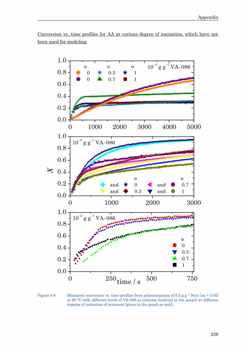
Appendix

259

Conversion vs. time profiles for AA at various degree of ionization, which have not

been used for modeling

0 1000 2000 3000 4000 50000.0

0.2

0.4

0.6

0.8

1.0

0 1000 2000 30000.0

0.2

0.4

0.6

0.8

1.0

0 250 500 7500.0

0.2

0.4

0.6

0.8

1.0

0 0.3 1

0 0.7 1

102

g g1

VA086

103

g g1

VA086

104

g g1

VA086

X

and 0 and 0.7

and 0.3 and 1

0

0.3

0.7

1

time / s

Figure 0-6 Measured conversion vs. time profiles from polymerization of 0.2 g g1 NaA (xM = 0.05)

at 90 °C with different levels of VA-086 as initiator (indicted in the graph) at different

degrees of ionization of monomer (given in the graph as well).

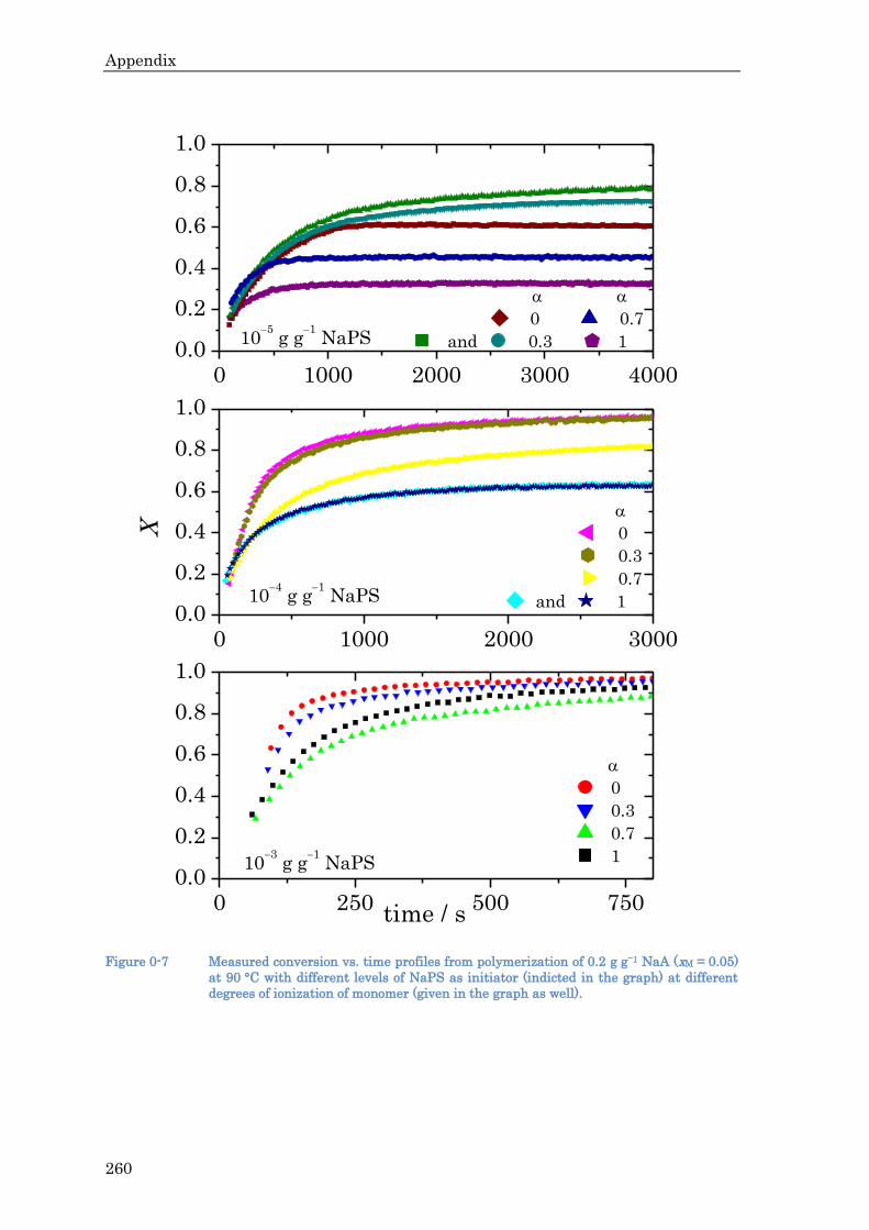
Appendix

260

0 1000 2000 3000 40000.0

0.2

0.4

0.6

0.8

1.0

0 1000 2000 30000.0

0.2

0.4

0.6

0.8

1.0

0 250 500 7500.0

0.2

0.4

0.6

0.8

1.0

103

g g1

NaPS

105

g g1

NaPS

104

g g1

NaPS

X

0 0.7

and 0.3 1

0

0.3

0.7

and 1

0

0.3

0.7

1

time / s

Figure 0-7 Measured conversion vs. time profiles from polymerization of 0.2 g g1 NaA (xM = 0.05)

at 90 °C with different levels of NaPS as initiator (indicted in the graph) at different

degrees of ionization of monomer (given in the graph as well).

Appendix

261

Appendix

263

Abbreviations and Symbols

A Arrhenius pre-exponential factor

A pressure-independent Arrhenius pre-exponential factor

D-HA 1st Debye–Hückel parameter (not empirical)

Å 1010 m

AA acrylic acid

AAm acrylamide

apt attached proton test (NMR technique)

at acquisition time

D-HB 2nd Debye–Hückel parameter (empirical)

BA butyl acrylate

bb backbiting

BP branching point

bs broad singlet

bt broad triplet

xC carbon, index p: primary, s: secondary, t: tertiary, q:quaternary

y

xC chain transfer constant (x giving species to which transfer occurs, y giving

of type of radical: s – secondary, t – tertiary)

D-HC 3rd Debye–Hückel parameter (empirical)

y

xc concentration (x giving species, y giving time)

ca. circa, Latin: around/about

CLD chain-length distribution

CLDP chain-length-dependent propagation

CLDT chain-length-dependent termination

XD diffusion coefficient of species X

Ð dispersity

D1173 2-hydroxy-2-methyl-1-phenylpropan-1-one

dept-135 distortionless enhancement by polarization transfer 135 degree (NMR

technique)

DiAA diacrylic acid (2-(acryloyloxy)acetic acid)

DMSO dimethyl sulfoxide

DTBP di-tert-butyl peroxide

E energy (an index of A refers to activation, an index of P to laser pulse, an

index of tomolar energy of photons at given laser wavelength)

e.g. exempli gratia, Latin: for example

EPR electron paramagnetic resonance

et al. et alii / et aliae, Latin: and others

eq. equation

f fraction of initiator fragments available for initiation

FID free induction decay

FT Fourier transform

H-A acid (general)

HPLC high-performance liquid chromatography

h empirical parameter of the extended Henderson–Hasselbalch equation

I ionic strength

i molecular species

i chain length or running index; chevron indicates: averaged, i.e. degree of

polymerization, index of n indicates: nuber-averaged

Appendix

265

IBA iso-butyric acid

i.e. id est, Latin: that is

j chain length or running index

HK protonation constant, subscript indicates corresponding degree of

ionization of polymer

Bk Boltzmann constant

y

xk rate coefficient (x giving reaction: bb – backbiting, d – (initiator)

dissociation, i – initiation, p – propagation, t – termination <may be

further specified after comma D: diffusion, C: chemical reaction>, tr,X –

transfer to species X; y giving time or chain length of involved polymer

species or of type of radical(s): s – secondary, t – tertiary), chevron indicate:

chain-length averaged, superscript zero denotes: at time zero/zero

conversion

l length, index p: persistence (chain) length, 0: persistence (chain) length

without electronic influence, e: electronic persistence (chain) length

lg decadic logarithm

LHS left-handed side

M monomer

nM number average molar mass

wM weight average molar mass

xM molar mass of species x

MAA methacrylic acid

MALDI matrix-assisted laser desorption ionization

MCR midchain radical (s: formed by an 1,5-hydrogen shift; l: not (directly) formed

by an 1,5-hydrogen shift )

ME 2-mercaptoethanol

MeHQ hydroquinone monomethyl ether

MM macromonomer

MMA methyl methacrylate

MMD molar-mass distribution

MMMP 2-methyl-4-(methylthio)-2-morpholino-propiophenone

MS mass spectrometry

MU monomer unit

y

xn quantity (amount) of species x at time y

NaA sodium acrylate = fully ionized acrylic acid with sodium counter ion

NaMA sodium methacrylate = fully ionized methacrylic acid with sodium counter

ion

NaPS sodium persulfate

NIR near infrared

NOE nuclear Overhauser effect

Pi dead polymer chain with a chain length of i

P radiant power (index 0 means: in front of cell)

p propagation

p pressure

pAA poly(acrylic acid)

pAAm poly(acrylamide)

pBA poly(butyl acrylate)

PLP pulsed laser polymerization

pMAA poly(methacrylic acid)

polym polymerization (used as index)

pVP polyvinylpyrrolidone

xQ partition function of species X (index of ‡ indicates activated complex)

Appendix

267

Ri

growing polymer chain with a chain length of i (dot indicates radical

species)

R rest of the molecule not depicted for reasons of space available (only used

in drawings of molecules)

R universal gas constant

r rate

rd relaxation delay

RHS right-handed side

RD reaction diffusion

SEC size exclusion chromatography

S/N signal-to-noise

SD segmental diffusion

SP single pulse

SPR secondary propagating radical

T absolute temperature (in kelvin)

t time

TEMPO 2,2,6,6-tetramethylpiperidine 1-oxyl

TD translational diffusion

ToF time-of-flight

V molar volume, index 0 indicates extrapolated to infinite dilution

V-50 2-[(E)-2-(1-carbamimidoyl-1-methylethyl)diazen-1-yl]-2-methylpropan-

imidamide dihydrochloride

VA-086 2,2'-Azobis[2-methyl-N-(2-hydroxyethyl)propionamide]

v.i. vide infra, Latin: see below

viz. videre licit, Latin: it is permitted to see (namely)

v.s. vide supra, Latin: see above

xw weight fraction of x

X arbitrary species (with dot: arbitrary radical species)

YX degree of conversion, index gives species; without index it refers to

monomer

xx mole fraction of x

Y arbitrary species (with dot arbitrary radical species)

z charge number

degree of ionization

l exponent of chain-length dependency in region of long chains

s exponent of chain-length dependency in region of short chains

‡V activation volume

kinetic chain length

chemical shift (only if referring to NMR)

molar decadic absorption coefficient

correction factor for tk ; superscript: s stands for secondary radical, t

stands for tertiary radical; subscript: d stands for distribution (correcting a

value for one chain length to use it for a distribution, which average chain

length is the former one), w stands for correction of viscosity change with

different monomer content, stands for correction of viscosity change

with ionization, C stands for correction of Coulomb repulsion of ionized

macroradicals

dynamic viscosity, subscript r: relative, superscript X: at conversion X

temperature in °C

fraction of disproportionation, index gives type of radical terminating:

s:secondary, t:tertiary

slope of first CLD plot

wavenumber

Appendix

269

kinematic viscosity

I correction factor for influence of additional salt on pk

density

transmission coefficient

residence time, index: calc: calculated from mass flow, density of the

reaction mixture and geometric volume of the reactor.

radiant power (intensity) at a certain wavenumber

References

271

References

[1] Staudinger, H.; Fritschi, J. Helv. Chim. Acta. 1922, 5, 785–806.

[2] Staudinger, H. Ber. dtsch. Chem. Ges. A/B 1920, 53, 1073–1085.

[3] Baekeland, L. H., US patent No. 942699, 1909.

[4] Verband der Chemischen Industrie e.V., Chemiewirtschaft in Zahlen 2013,

2013.

[5] Olaj, O. F.; Bitai, I.; Hinkelmann, F. Makromol. Chem. 1987, 188, 1689–1702.

[6] Buback, M.; Hippler, H.; Schweer, J.; Voegele, H. P. Makromol. Chem. Rapid

Commun. 1986, 7, 261–265.

[7] Buback, M.; Egorov, M.; Junkers, T.; Panchenko, E. Macromol. Rapid

Commun. 2004, 25, 1004–1009.

[8] Beuermann, S.; Buback, M.; Hesse, P.; Kuchta, F.-D.; Lacík, I.; van

Herk, A. M. Pure Appl. Chem. 2007, 79, 1463–1469.

[9] Beuermann, S.; Buback, M.; Hesse, P.; Kukučková, S.; Lacík, I. Macromol.

Symp. 2007, 248, 41–49.

[10] Beuermann, S. Macromol. Rapid Commun. 2009, 30, 1066–1088.

[11] Lacík, I.; Učňovaá, L.; Kukučková, S.; Buback, M.; Hesse, P.; Beuermann, S.

Macromolecules 2009, 42, 7753–7761.

[12] Kabanov, V. A.; Topchiev, D. A.; Karaputadze, T. M. J. Polym. Sci. Pol. Sym.

1973, 42, 173–183.

[13] Giese, B. Angew. Chem. 1983, 95, 771–782.

References

272

[14] IUPAC, http://goldbook.iupac.org/, accessed: February 2013.

[15] Russell, K.; Tobolsky, A. J. Am. Chem. Soc. 1953, 75, 5052–5054.

[16] Pryor, W. A.; Lasswell, L. D. Adv. free-radical chem. 1975, 5, 27.

[17] Kharasch, F. R., M. S.; Mayo Chem. Ind. 1938, 57, 752.

[18] Bouguer, P. Essai d’Optique, sur la gradation de la lumiere; Claude Jombert:

Paris, 1729; pp 63–67.

[19] Lambert, J. H. Photometria sive de Mensura et Gradibus Luminis, Colorum

et Umbrae; Eberhard Klett: Augsburg, 1760; p 391.

[20] Beer, A. Ann. Physik Chemie 1852, 86, 78–88.

[21] Buback, M.; Gilbert, R. G.; Russell, G. T.; Hill, D. J. T.; Moad, G.;

O’Driscoll, K. F.; Shen, J.; Winnik, M. A. J. Polym. Sci. A Polym. Chem. 1992,

30, 851–863.

[22] Hutchinson, R. A.; Paquet, D. A.; McMinn, J. H. Macromolecules 1995, 28,

5655–5663.

[23] Heuts, J. P. A.; Davis, T. P.; Russell, G. T. Macromolecules 1999, 32, 6019–

6030.

[24] Loubat, C.; Boutevin, B. Polym. Int. 2001, 50, 375–380.

[25] Bordwell, F. G.; Zhang, X.-M.; Satish, A. V.; Cheng, J.-P. J. Am. Chem. Soc.

1994, 116, 6605–6610.

[26] Mayo, F. R. J. Am. Chem. Soc. 1943, 65, 2324–2329.

[27] Whang, B. Y. C.; Ballard, M. J.; Napper, D. H.; Gilbert, R. G. Aust. J. Chem.

1991, 44, 1133.

[28] O’Brien, J. L.; Gornick, F. J. Am. Chem. Soc. 1955, 77, 4757–4763.

[29] Moad, G.; Moad, C. L. Macromolecules 1996, 29, 7727–7733.

[30] Suddaby, K. G.; Maloney, D. R.; Haddleton, D. M. Macromolecules 1997, 30,

702–713.

[31] Buback, M.; Laemmel, R. A. Macromol. Theory Simul. 1997, 6, 145–150.

[32] Roedel, M. J. J. Am. Chem. Soc. 1953, 75, 6110–6112.

References

273

[33] Toh, J. S. S.; Huang, D. M.; Lovell, P. A.; Gilbert, R. G. Polymer 2001, 42,

1915–1920.

[34] Cuccato, D.; Mavroudakis, E.; Dossi, M.; Moscatelli, D. Macromol. Theory

Simul. 2013, 22, 127–135.

[35] Staudinger, H.; Schulz, G. V. Ber. dtsch. Chem. Ges. A/B 1935, 68, 2320–

2335.

[36] Barth, J.; Meiser, W.; Buback, M. Macromolecules 2012, 45, 1339–1345.

[37] Lacík, I.; Beuermann, S.; Buback, M. Macromolecules 2003, 36, 9355–9363.

[38] Nikitin, A. N.; Hutchinson, R. A. Macromolecules 2005, 38, 1581–1590.

[39] Cuccato, D.; Dossi, M.; Moscatelli, D.; Storti, G. Macromol. React. Eng. 2012,

6, 330–345.

[40] Liang, K.; Hutchinson, R. A. Macromol. Rapid Commun. 2011, 32, 1090–1095.

[41] Liang, K.; Hutchinson, R. A.; Barth, J.; Samrock, S.; Buback, M.


[42] Nikitin, A. N.; Hutchinson, R. A.; Wang, W.; Kalfas, G. A.; Richards, J. R.;

Bruni, C. Macromol. React. Eng. 2010, 4, 691–706.

[43] Wang, W.; Nikitin, A. N.; Hutchinson, R. A. Macromol. Rapid Commun. 2009,

30, 2022–2027.

[44] Engler, C.; Weißberg, J. Kritische Studien über die Vorgänge der

Autoxydation; 1904; p 179.

[45] Schulz, V. G. V.; Henrici, G. Makromol. Chem. 1956, 18, 437–454.

[46] Gladyshev, G. Proc. Acad. Sci. USSR 1974, 215, 898–901.

[47] Kern, V. W. Makromol. Chem. 1948, 1, 199–208.

[48] Russell, G. T.; Napper, D. H.; Gilbert, R. G. Macromolecules 1988, 21, 2133–

2140.

[49] Nikitin, A. N.; Grady, M. C.; Kalfas, G. A.; Hutchinson, R. A. Macromol.

React. Eng. 2008, 2, 422–435.

[50] von Smoluchowski, M. Z. Phys. Chem 1917 92, 129–168.

References

274

[51] Einstein, A. Ann. Phys. 1905, 17, 549–560.

[52] Van’t Hoff, J. H. Études de dynamique chimique; Frederik Muller & Co:

Amsterdam, 1884; pp 114–118.

[53] Arrhenius, S. Z. Phys. Chem. 1889, 4, 226–248.

[54] Ewell, R. H.; Eyring, H. J. Chem. Phys. 1937, 5, 726–737.

[55] Powell, R. E.; Roseveare, W. E.; Eyring, H. Ind. Eng. Chem. 1941, 33, 430–

435.

[56] Henton, D. E.; Powell, C.; Reim, R. E. J. Appl. Polym. Sci. 1997, 64, 591–600.

[57] Kuchta, F.-D.; van Herk, A. M.; German, A. L. Macromolecules 2000, 33,

3641–3649.

[58] Beuermann, S.; Paquet, D. A.; McMinn, J. H.; Hutchinson, R. A.


[59] Beuermann, S.; Buback, M.; Hesse, P.; Lacík, I. Macromolecules 2006, 39,

184–193.

[60] Eyring, H. J. Chem. Phys. 1935, 3, 107–115.

[61] Eyring, H.; Polanyi, M. Z. Phys. Chem. B 1931, 12, 279–311.

[62] Heuts, J. P. A.; Gilbert, R. G.; Radom, L. Macromolecules 1995, 28, 8771–

8781.

[63] Thickett, S. C.; Gilbert, R. G. Polymer 2004, 45, 6993–6999.

[64] Degirmenci, I.; Ozaltin, T. F.; Karahan, O.; Van Speybroeck, V.;

Waroquier, M.; Aviyente, V. J. Polym. Sci. A Polym. Chem. 2013, 51, 2024–

2034.

[65] De Sterck, B.; Vaneerdeweg, R.; Du Prez, F.; Waroquier, M.;

Van Speybroeck, V. Macromolecules 2009, 43, 827–836.

[66] Stach, M.; Lacík, I.; Chorvákt, D.; Buback, M.; Hesse, P.; Hutchinson, R. A.;

Tang, L. Macromolecules 2008, 41, 5174–5185.

[67] Stach, M.; Lacík, I.; Kasák, P.; Chorv/’akt, D.; Saunders, A. J.;

Santanakrishnan, S.; Hutchinson, R. A. Macromol. Chem. Phys. 2010, 211,

580–593.

References

275

[68] Ito, H.; Shimizu, A. J. Chem. Soc. Japan, Ind. Chem. Sect 1955, 58, 194.

[69] Kabanov, V.; Topchiev, D.; Karaputadze, T.; Mkrtchian, L. Eur. Polym. J.

1975, 11, 153–159.

[70] Manickam, S.; Venkatarao, K.; Subbaratnam, N. Eur. Polym. J. 1979, 15,

483–487.

[71] Plochocka, K. J. Macromol. Sci., Rev. Macromol. Chem. Phys. 1981, 20, 67–

148.

[72] Pinner, S. H. J. Polym. Sci. 1952, 9, 282–285.

[73] Blauer, G. J. Polym. Sci. 1953, 11, 189–192.

[74] Scott, R. A.; Peppas, N. A. AIChE Journal 1997, 43, 135–144.

[75] Rintoul, I.; Wandrey, C. Polymer 2005, 46, 4525–4532.

[76] Lacík, I.; Beuermann, S.; Buback, M. Macromol. Chem. Phys. 2004, 205,

1080–1087.

[77] Barth, J.; Buback, M. Macromolecules 2012, 45, 4152–4157.

[78] Anseth, K. S.; Scott, R. A.; Peppas, N. A. Macromolecules 1996, 29, 8308–

8312.

[79] Shoaf, G. L.; Poehlein, G. W. J. Appl. Polym. Sci. 1991, 42, 1239–1257.

[80] Cutié, S. S.; Smith, P. B.; Henton, D. E.; Staples, T. L.; Powell, C. J. Polym.

Sci. B Polym. Phys. 1997, 35, 2029–2047.

[81] De Stefano, C.; Gianguzza, A.; Piazzese, D.; Sammartano, S. React. Funct.

Polym. 2003, 55, 9–20.

[82] Laguecir, A.; Ulrich, S.; Labille, J.; Fatin-Rouge, N.; Stoll, S.; Buffle, J. Eur.

Polym. J. 2006, 42, 1135–1144.

[83] Katchalsky, A.; Blauer, G. Trans. Faraday Soc. 1951, 47, 1360–1370.

[84] Tricot, M. Macromolecules 1984, 17, 1698–1704.

[85] Mylonas, Y.; Staikos, G.; Ullner, M. Polymer 1999, 40, 6841–6847.

[86] Adamczyk, Z.; Bratek, A.; Jachimska, B.; Jasinski, T.; Warszynski, P. J. Phys.

Chem. B 2006, 110, 22426–22435.

References

276

[87] Dobrynin, A. V.; Rubinstein, M. Prog. Polym. Sci. 2005, 30, 1049–1118.

[88] Breslau, B. R.; Miller, I. F. J. Phys. Chem. 1970, 74, 1056–1061.

[89] Olaj, O.; Schnöll-Bitai, I. Eur. Polym. J. 1989, 25, 635–641.

[90] Buback, M.; Hesse, P.; Hutchinson, R. A.; Kasak, P.; Lacík, I.; Stach, M.;

Utz, I. Ind. Eng. Chem. Res. 2008, 47, 8197–8204.

[91] Lacík, I.; Beuermann, S.; Buback, M. Macromolecules 2001, 34, 6224–6228.

[92] Beuermann, S.; Buback, M.; Hesse, P.; Kukučková, S.; Lacík, I. Macromol.

Symp. 2007, 248, 23–32.

[93] Piton, M. C.; Gilbert, R. G.; Chapman, B. E.; Kuchel, P. W. Macromolecules

1993, 26, 4472–4477.

[94] De Gennes, P.; Leger, L. Annu. Rev. Phys. Chem. 1982, 33, 49–61.

[95] Tsvetkov, V.; Kolomiets, I.; Lezov, A. Soedin., Ser. A 1968, 10, 74.

[96] Smith, G. B.; Heuts, J. P.; Russell, G. T. Macromol. Symp. 2005, 226, 133–

146.

[97] Smith, G. B.; Russell, G. T.; Heuts, J. P. Macromol. Theory Simul. 2003, 12,

299–314.

[98] Buback, M.; Egorov, M.; Junkers, T.; Panchenko, E. Macromol. Chem. Phys.

2005, 206, 333–341.

[99] Buback, M.; Müller, E.; Russell, G. T. J. Phys. Chem. A 2006, 110, 3222–3230.

[100] Barth, J.; Buback, M.; Hesse, P.; Sergeeva, T. Macromolecules 2009, 42, 481–

488.

[101] Barth, J.; Buback, M.; Hesse, P.; Sergeeva, T. Macromol. Rapid Commun.

2009, 30, 1969–1974.

[102] Barth, J.; Buback, M.; Schmidt-Naake, G.; Woecht, I. Polymer 2009, 50, 5708–

5712.

[103] Barth, J.; Buback, M. Macromol. Rapid Commun. 2009, 30, 1805–1811.

[104] Khokhlov, A. R. Makromol. Chem. Rapid Commun. 1981, 2, 633–636.

[105] Olaj, O. F.; Zifferer, G. Makromol. Chem. Rapid Commun. 1982, 3, 549–556.

References

277

[106] Friedman, B.; O’Shaughnessy, B. Macromolecules 1993, 26, 5726–5739.

[107] Barner-Kowollik, C.; Russell, G. T. Prog. Polym. Sci. 2009, 34, 1211–1259.

[108] Buback, M.; Junkers, T. Macromol. Chem. Phys. 2006, 207, 1640–1650.

[109] Taylor, D. R.; van Berkel, K. Y.; Alghamdi, M. M.; Russell, G. T. Macromol.

Chem. Phys. 2010, 211, 563–579.

[110] Schuh, H.; Fischer, H. Helv. Chim. Acta. 1978, 61, 2130–2164.

[111] Buback, M.; Busch, M.; Kowollik, C. Macromol. Theory Simul. 2000, 9, 442–

452.

[112] Theis, A.; Davis, T. P.; Stenzel, M. H.; Barner-Kowollik, C. Macromolecules

2005, 38, 10323–10327.

[113] Johnston-Hall, G.; Stenzel, M. H.; Davis, T. P.; Barner-Kowollik, C.;

Monteiro, M. J. Macromolecules 2007, 40, 2730–2736.

[114] Johnston-Hall, G.; Monteiro, M. J. J. Polym. Sci. A Polym. Chem. 2008, 46,

3155–3173.

[115] Johnston-Hall, G.; Monteiro, M. J. Macromolecules 2008, 41, 727–736.

[116] Olaj, O. F.; Vana, P.; Zoder, M.; Kornherr, A.; Zifferer, G. Macromol. Rapid

Commun. 2000, 21, 913–920.

[117] Willemse, R. X. E.; Staal, B. B. P.; van Herk, A. M.; Pierik, S. C. J.;

Klumperman, B. Macromolecules 2003, 36, 9797–9803.

[118] Smith, G. B.; Russell, G. T.; Yin, M.; Heuts, J. P. Eur. Polym. J. 2005, 41,

225–230.

[119] Johnston-Hall, G.; Theis, A.; Monteiro, M. J.; Davis, T. P.; Stenzel, M. H.;

Barner-Kowollik, C. Macromol. Chem. Phys. 2005, 206, 2047–2053.

[120] Barth, J.; Buback, M. Macromolecules 2011, 44, 1292–1297.

[121] Beuermann, S.; Buback, M.; Hesse, P.; Hutchinson, R. A.; Kukučková, S.;

Lacík, I. Macromolecules 2008, 41, 3513–3520.

[122] Benson, S. W.; North, A. M. J. Am. Chem. Soc. 1959, 81, 1339–1345.

[123] Benson, S. W.; North, A. M. J. Am. Chem. Soc. 1962, 84, 935–940.

References

278

[124] R. G. W. Norrish, R. R. S. Nature 1942, 150, 336–337.

[125] Trommsdorff, V. E.; Köhle, H.; Lagally, P. Makromol. Chem. 1948, 1, 169–

198.

[126] Soh, S.; Sundberg, D. J. Polym. Sci. Polym. Chem. Ed. 1982, 20, 1315–1329.

[127] Buback, M.; Schweer, J. Z. Phys. Chem. 1989, 161, 153–165.

[128] Allen, P.; Patrick, C. Makromol. Chem. 1964, 72, 106–118.

[129] Buback, M.; Degener, B. Makromol. Chem. 1993, 194, 2875–2883.

[130] Buback, M.; Huckestein, B.; Russell, G. T. Macromol. Chem. Phys. 1994, 195,

539–554.

[131] Ballard, M. J.; Napper, D. H.; Gilbert, R. G. J. Polym. Sci. Polym. Chem. Ed.

1984, 22, 3225–3253.

[132] Carswell, T.; Hill, D.; Londero, D.; O’Donnell, J.; Pomery, P.; Winzor, C.

Polymer 1992, 33, 137–140.

[133] Zetterlund, P. B.; Yamazoe, H.; Yamada, B.; Hill, D. J.; Pomery, P. J.


[134] Zetterlund, P. B.; Yamazoe, H.; Yamada, B. Macromol. Theory Simul. 2003,

12, 379–385.

[135] Zetterlund, P. B.; Yamauchi, S.; Yamada, B. Macromol. Chem. Phys. 2004,

205, 778–785.

[136] Buback, M. Makromol. Chem. 1990, 191, 1575–1587.

[137] Wulkow, M. Macromol. Theory Simul. 1996, 5, 393–416.

[138] Wampler III, F. M. Plant/Operations Progress 1988, 7, 183–189.

[139] Acrylic Acid Dimerization; Technical Report, 1997, Technical Data Sheet.

[140] Buback, M. Angew. Chem. 1991, 103, 658–670.

[141] Beuermann, S.; Buback, M.; Hesse, P.; Junkers, T.; Lacík, I. Macromolecules

2006, 39, 509–516.

[142] NIST, Webbook, 2008. webbook.nist.gov/chemistry/.

[143] Barth, J. Ph.D. thesis, Georg-August-Universität Göttingen, 2011.

References

279

[144] Hesse, P. Ph.D. thesis, Universität Göttingen, 2008.

[145] Schrooten, J. Ph.D. thesis, Georg-August-Universität Göttingen, 2013.

[146] Handbook of Chemistry and Physics - 84th Edition -; Lide, D. R., Ed.; CRC

press, 2003; pp 8/–43.

[147] Wittenberg, N. F. G. Diplomarbeit, Georg-August-Universität Göttingen,

2009.

[148] Weiß, D. M.Sc. thesis, Georg-August-Universität Göttingen, 2012.

[149] van Herk, A. M. J. Chem. Educ. 1995, 72, 138–.

[150] Van Herk, A. M.; Dröge, T. Macromol. Theory Simul. 1997, 6, 1263–1276.

[151] Beuermann, S.; Buback, M.; Davis, T. P.; Gilbert, R. G.; Hutchinson, R. A.;

Olaj, O. F.; Russell, G. T.; Schweer, J.; van Herk, A. M. Macromol. Chem.

Phys. 1997, 198, 1545–1560.

[152] Henríquez, C.; Bueno, C.; Lissi, E. A.; Encinas, M. V. Polymer 2003, 44, 5559

– 5561.

[153] Nikitin, A. N.; Castignolles, P.; Charleux, B.; Vairon, J.-P. Macromol. Rapid

Commun. 2003, 24, 778–782.

[154] Hutchinson, R. A.; Aronson, M. T.; Richards, J. R. Macromolecules 1993, 26,

6410–6415.

[155] Husain, M. M.; Misra, S. N.; Miss, A. G. Makromol. Chem. 1976, 177, 2919–

2926.

[156] Information provided by Wako Chemicals GmbH on request.

[157] Kukučková, S. Ph.D. thesis, Bratislava/Göttingen, 2006.

[158] Olaj, O. F.; Zifferer, G.; Gleixner, G. Makromol. Chem. Rapid Commun. 1985,

6, 773–784.

[159] Mahabadi, H. K. Macromolecules 1985, 18, 1319–1324.

[160] Olaj, O. F.; Zifferer, G.; Gleixner, G. Macromolecules 1987, 20, 839–850.

[161] Mahabadi, H. K. Macromolecules 1991, 24, 606–609.

References

280

[162] Wittenberg, N. F. G.; Buback, M.; Stach, M.; Lacík, I. Macromol. Chem. Phys.

2012, 213, 2653–2658.

[163] Sarraguça, J.; Pais, A. Chem. Phys. Lett. 2004, 398, 140–145.

[164] Masiak, M.; Hyk, W.; Stojek, Z.; Ciszkowska, M. J. Phys. Chem. B 2007, 111,

11194–11200.

[165] Sakurai, M.; Imai, T.; Yamashita, F.; Nakamura, K.; Komatsu, T. and

Nakagawa, l. T. Polym. J. 1993, 25, 1247–1255.

[166] Taylor, T. J.; Stivala, S. S. J. Polym. Sci. B Polym. Phys. 2003, 41, 1263–1272.

[167] Gromov, V.; Galperina, N.; Osmanov, T.; Khomikovskii, P.; Abkin, A. Eur.

Polym. J. 1980, 16, 529–535.

[168] Paril, A.; Alb, A.; Giz, A.; Çatalgil Giz, H. J. Appl. Polym. Sci. 2007, 103, 968–

974.

[169] Deglmann, P.; Müller, I.; Becker, F.; Schäfer, A.; Hungenberg, K.-D.; Weiß, H.

Macromol. React. Eng. 2009, 3, 496–515.

[170] Torii, H.; Fujimoto, K.; Kawaguchi, H. J. Polym. Sci. A Polym. Chem. 1996,

34, 1237–1243.

[171] BASF Corporation, Acrylic Acid Glacial (Technical Data Sheet); Technical

Report, 2001.

[172] The Dow Chemical Company, Acrylic Acid, Glacial (Technical Data Sheet);

Technical Report.

[173] Günzler, K. F. Ph.D. thesis, Georg-August-Universität Göttingen, 2007.

[174] Nikitin, A. N.; Hutchinson, R. A.; Kalfas, G. A.; Richards, J. R.; Bruni, C.

Macromol. Theory Simul. 2009, 18, 247–258.

[175] Loiseau, J.; Doërr, N.; Suau, J. M.; Egraz, J. B.; Llauro, M. F.; Ladavière, C.;

Claverie, J. Macromolecules 2003, 36, 3066–3077.

[176] Junkers, T.; Koo, S. P. S.; Davis, T. P.; Stenzel, M. H.; Barner-Kowollik, C.


[177] Castignolles, P.; Graf, R.; Parkinson, M.; Wilhelm, M.; Gaborieau, M. Polymer

2009, 50, 2373–2383.

References

281

[178] Barth, J.; Buback, M.; Hesse, P.; Sergeeva, T. Macromolecules 2010, 43,

4023–4031.

[179] Ahmad, N. M.; Heatley, F.; Lovell, P. A. Macromolecules 1998, 31, 2822–2827.

[180] de la Fuente, J. L.; López Madruga, E. Macromol. Chem. Phys. 2001, 202,

375–381.

[181] Plessis, C.; Arzamendi, G.; Alberdi, J. M.; van Herk, A. M.; Leiza, J. R.;

Asua, J. M. Macromol. Rapid Commun. 2003, 24, 173–177.

[182] Agirre, A.; Santos, J. I.; Etxeberria, A.; Sauerland, V.; Leiza, J. R. Polym.

Chem. 2013, 4, 2062–2079.

[183] Handbook of Chemistry and Physics - 84th Edition -; Lide, D. R., Ed.; CRC

press, 2003; pp 9/–51.

[184] Beuermann, S.; Buback, M. Prog. Polym. Sci. 2002, 27, 191–254.

[185] Nikitin, A. N.; Hutchinson, R. A. Macromol. Theory Simul. 2006, 15, 128–136.

[186] Gao, Z.; Amasaki, I.; Kaneko, T.; Nakada, M. Polym. Degrad. Stab. 2003, 81,

125–130.

[187] Noda, I.; Tsuge, T.; Nagasawa, M. J. Phys. Chem. 1970, 74, 710–719.

[188] Debye, P.; Hückel, E. Physik. Z. 1923, 24, 185–206.

[189] Archer, D. G.; Wang, P. J. Phys. Chem. Ref. Data 1990, 19, 371–412.

[190] Hiraoka, K.; Yokoyama, T. J. Polym. Sci. B Polym. Phys. 1986, 24, 769–778.

[191] Conway, B. E.; Laliberte, L. H. Trans. Faraday Soc. 1970, 66, 3032–3047.

[192] Gianni, P.; Lepori, L. J. Solution Chem. 1996, 25, 1–42.

[193] Barta, L.; Hepler, L. G. J. Phys. Chem. 1989, 93, 5588–5595.

[194] Hiraoka, K.; Shin, H.; Yokoyama, T. Polym. Bull. 1982, 8, 303–309.

[195] Smith, M. Organic Chemistry: An Acid Base Approach; CRC Press, 2011; p

214.

[196] Handbook of Chemistry and Physics - 84th Edition -, 84th ed.; Linde, D. R.,

Ed.; CRC Press, 2004; pp 8/–47.

References

282

[197] Arnold, R.; Ticktin, S.; Monseair, G.; Stephen, A. M. J. Chem. Soc. 1963, 0,

5810–5815.

[198] Soni, M. L.; Kapoor, R. C. Int. J. Quantum Chem. 1981, 20, 385–391.

[199] Dewick, P. M. Essentials of Organic Chemistry: For Students of Pharmacy,

Medicinal Chemistry and Biological Chemistry; John Wiley & Sons, 2013; p

144.

[200] Pines, E.; Magnes, B.-Z.; Lang, M. J.; Fleming, G. R. Chem. Phys. Lett. 1997,

281, 413–420.

[201] Kolthoff, I. M.; Miller, I. K. J. Am. Chem. Soc. 1951, 73, 3055–3059.

[202] Mahdavian, A.; Abdollahi, M.; Bijanzadeh, H. R. J. Appl. Polym. Sci. 2004, 93,

2007–2013.

[203] Seabrook, S. A.; Tonge, M. P.; Gilbert, R. G. J. Polym. Sci. A Polym. Chem.

2005, 43, 1357–1368.

[204] Pascal, P.; Winnik, M. A.; Napper, D. H.; Gilbert, R. G. Macromolecules 1993,

26, 4572–4576.

[205] Seabrook, S. A.; Pascal, P.; Tonge, M. P.; Gilbert, R. G. Polymer 2005, 46,

9562–9573.

Danksagung/Acknowledgements

Mein außerordentlicher Dank gilt Herrn Prof. Dr. M. Buback für die interessante

Themenstellung sowie die stete Diskussionsbereitschaft und Förderung dieser

Arbeit.

Außerdem bedanke ich mich bei Prof. Dr. P. Vana, MBA für die Übernahme des

Korreferats.

Special thanks go to Prof. Robin A. Hutchinson (Queen’s University, Canada) for

inviting me to Canada and introducing me to modeling, lots of helpful discussions

and suggestions, and altogether a very fruitful cooperation.

I thank Igor Lacík, DSc, and Marek Stach, PhD, (Polymer Institute SAV, Slovakia)

for discussions providing insight into challenging SEC analyses, and determination

of many MMDs. Contributions of further coworkers at the Polymer Institute of the

Slovak Academy of Sciences in Bratislava are also gratefully acknowledged.

Ďakujem.

I thank Sandhya Santanakrishnan, PhD, for help with Predici and showing me

around at Queen’s.

I’d like to thank Calista Preusser (Queen’s University, Canada) for interesting

discussion and for sharing results.

Ein besonderer Dank gebührt Dr. Jens Schrooten, Dr. Johannes Barth, Hendrik

Kattner, Henrik Schröder und Patrick Drawe für ihre unermüdliche

Diskussionsbereitschaft und viele hilfreiche Anregungen.

Weiterer Dank gilt Herrn Dr. H.-P. Vögele für die ständige Hilfsbereitschaft bei

technischen Fragen, besonders zu den IR-Spektrometern.

Bei Herrn R. Machinek bedanke ich mich für Ratschläge zur NMR-Messung und

tatkräftige Hilfe beim Finden der richtigen Messbedingungen, sowie bei der

gesamten NMR-Abteilung für die Messung von NMR-Proben.

Herrn Dr. H. Frauendorf danke ich für die MS-ESI und HPLC Messungen sowie

hilfreiche Anmerkungen.

I wish to thank Dr. Tatiana Sergeeva for discussions and support regarding

evaluation of EPR spectra as well as for sharing results.

Ich danke Patrick Drawe und Dr. Johannes Barth für das Teilen von Ergebnissen.

Großer Dank gebührt Dr. Johannes Buback für das Programm Predici Batch, eine

exzellente Ergänzung des Programms PREDICITM.

Ich danke Daniel Weiß, dessen Masterarbeit ich mitbetreut habe, für die gute

Zusammenarbeit und das Teilen von Ergebnissen.

Ich danke Justus B. Söllner und Roman Kremring, deren Bachelorarbeiten ich

betreut habe, für die Zusammenarbeit.

I thank Dr. Hugo Vale (BASF SE) for helpful discussions and suggestions.

Herrn Prof. Dr. F. Meyer möchte ich für die Bereitstellung des ESR-Spektrometers

danken.

Thanks are given to Prof. Dr. Alex M. van Herk (Technische Universiteit Eindhoven,

the Netherlands) for providing the program Contour.

Den Mitarbeitern der Institutswerkstätten danke ich für ihre Hilfsbereitschaft und

zuverlässige Arbeit.

Ich möchte mich bei Patrick Drawe, Henrik Schröder, Julia Möhrke, Hendrik

Kattner, Nicolai Sörensen, Dennis Hübner und Jan-Hendrik Schütz für das

Korrekturlesen dieser Arbeit bedanken.

Die Hilfe von Dr. Jens Schrooten bei der Bedienung des Lasers für PLP soll an

dieser Stelle dankend erwähnt werden.

Ich danke Cathrin Conrad und Björn Sölter dafür, dass sie Kaffeebohnen und Milch

für die Abteilungen eingekauft haben – ohne den Kaffee zwischendurch hätte ich es

nicht geschafft ;-)

Bei allen Mitgliedern der Arbeitskreise Buback und Vana bedanke ich mich für die

angenehme Arbeitsatmosphäre und die stete Hilfsbereitschaft, nicht zu vergessen

zahlreiche Frühstücke, Kuchen, Eis, aber auch gemeinsame Ausflüge zum

Kanufahren oder Wandern.

Bei der BASF SE möchte ich mich für die finanzielle Unterstützung dieser Arbeit

bedanken.

Ich danke dem Deutschen Akademischen Austauschdienst (DAAD) für die

finanzielle Unterstützung meines Aufenthaltes an der Queen’s University in

Kanada.

Abschließend möchte ich meinen Freunden, speziell der „Reisegruppe“, für die

moralische Unterstützung und die zahlreichen willkommenen Ablenkungen danken.

Ich danke meiner Freundin, dass sie meistens ;-) an mich geglaubt hat und immer

für mich da ist.

Mein größter Dank gilt meiner Familie. Für ihre Begleitung und Bestärkung, ihre

Geduld und ihr Vertrauen in mich bin ich ihnen zutiefst dankbar.

CURRICULUM VITAE

Personal Details

Name Nils Friedrich Gunter Wittenberg

Date and Place of Birth 1983/Nov/06 in Hamburg

Citizenship German

Education

2009/Oct–present doctoral dissertation research at Georg-August-

Universität Göttingen, workgroup Prof. M. Buback,

“Kinetics and Modeling of the Radical Polymerization

of Acrylic Acid and of Methacrylic Acid in Aqueous

Solution”

2010/May–2010/Jul research stay at Queen’s University in Kingston, ON,

Canada, workgroup Prof. R. Hutchinson

2004/Oct–2009/Aug diploma studies in chemistry at Georg-August-

Universität Göttingen

2009/Aug/12 Chemie-Diplom (graduation in chemistry)

2008/Oct–2009/Apr diploma thesis, workgroup Prof. M. Buback,

“Initiierung und Regelung bei radikalischer

(Meth)Acrylsäurepolymerisation in wässriger Lösung”

2010/May–2010/Jul research stay at University of New South Wales in

Kensington, NSW, Australia, workgroup Prof. R. Read

2003/Jun/26 Abitur at the Gymnasium Rissen, Hamburg

Scholarships

2010/May–2010/July DAAD (Deutscher Akademischer Austauschdienst) for

a research stay at Queen’s University in Kingston,

ON, Canada

kinetics and modeling of the radical polymerization of

Documents