FTL REPORT R86-7

AN EXPERIMENTAL AND THEORETICAL STUDY

OF THE ICE ACCRETION PROCESS

DURING ARTIFICIAL AND NATURAL

ICING CONDITIONS

Mark S. Kirby

and R. John Hansman, Jr.

rn1ii lk LMay 1986

FLIGHT TRANSPORTATION LABORATORY REPORT R86-7

AN EXPERIMENTAL AND THEORETICAL STUDY

OF THE ICE ACCRETION PROCESS

DURING ARTIFICIAL AND NATURAL ICING CONDITIONS

Mark Samuel Kirby

and

R. John Hansman, Jr.

May 1986

AN EXPERIMENTAL AND THEORETICAL STUDY

OF THE ICE ACCRETION PROCESS

DURING ARTIFICIAL AND NATURAL ICING CONDITIONS

ABSTRACT

Real-time measurements of ice growth during artificial andnatural icing conditions were conducted using an ultrasonicpulse-echo technique. This technique allows ice thickness tobe measured with an accuracy of ±0.5 mm; in addition, theultrasonic signal characteristics may be used to detect thepresence of liquid on the ice surface and hence discern wetand dry ice growth behaviour. Ice growth was measured on thestagnation line of a cylinder exposed to artificial icingconditions in the NASA Lewis Icing Research Tunnel, andsimilarly for a cylinder exposed in flight to natural icingconditions. Ice thickness was observed to increaseapproximately linearly with exposure time during the initialicing period. The ice accretion rate was found to vary withcloud temperature during wet ice growth, and liquid runbackfrom the stagnation region was inferred. A steady-stateenergy balance model for the icing surface was used tocompare heat transfer characteristics for icing wind tunneland natural icing conditions. Ultrasonic measurements of wetand dry ice growth observed in the Icing Research Tunnel andin flight were compared with icing regimes predicted by aseries of heat transfer coefficients. The heat transfermagnitude was generally inferred to be higher for the icingwind tunnel tests than for the natural icing conditionsencountered in flight. An apparent variation in the heattransfer magnitude was also observed for flights conductedthrough different natural icing cloud formations.

-2-

ACKNOWLEDGMENTS

This work was supported by the National Aeronautics and

Space Administration and the Federal Aviation Administrationunder Grants NGL-22-009-640 and NAG-3-666. Wind tunnel and

flight test facilities were provided by the NASA LangleyResearch Center.

-3-

TABLE OF CONTENTS

Abstract 2

Acknowledgements 3

Table of Contents 4

List of Figures 8

List of Tables .11

Nomenclature 12

1. INTRODUCTION 14

1.1 Overview 14

1.2 Aircraft Icing 15

1.3 Modeling The Ice Accretion Process 20

2. STEADY-STATE THERMODYNAMIC ANALYSIS OF

AN ICING SURFACE 26

2.1 Modes of Energy Transfer 26

2.2 Control Volume Analysis for an Icing Surface 27

2.2.1 Control Volume Mass Balance 29

i) Mass Balance for Dry Ice Growth 32

ii) Mass Balance for Wet Ice Growth 34

2.2.2 Control Volume Energy Balance 36

i) Energy Balance for Dry Ice Growth 37

ii) Energy Balance for Wet Ice Growth 38

iii) Stagnation Region Energy Balance

for Wet Ice Growth 39

-4-

iv) Threshold Condition for Transition from

Dry to Wet Ice Surface in Stagnation Region 42

2.3 Comparison of Heat Transfer Models 44

3. REAL-TIME MEASUREMENT OF ICE GROWTH USING

ULTRASONIC PULSE-ECHO TECHNIQUES 47

3.1 Ultrasonic Pulse-Echo Thickness Measurement 47

3.2 Ultrasonic Signal Characteristics for

Dry Ice Growth 50

3.3 Ultrasonic Signal Characteristics for

Wet Ice Growth 52

3.4 Summary 56

4. ICING OF A CYLINDER DURING ARTIFICIAL

ICING CONDITIONS 57

4.1 Overview 57

4.2 Experimental Apparatus 58

4.3 Icing Research Tunnel Installation and

Test Procedure 61

4.3.1 The Icing Research Tunnel 61

4.3.2 Cylinder Installation 63

4.3.3 Test Procedure 64

4.3.4 Test Icing Conditions 65

4.4 Experimental Measurements of Ice Growth During

Artificial Icing Conditions 66

4.4.1 Comparison of Ice Growth During Heavy and

Light Icing Conditions 67

-5-

i) Effect of Exposure Time on Icing Rate 70

ii) Comparison of Ice Accretion Rates for

Heavy and Light Icing Conditions 73

iii) Effect of Cloud Temperature on Ice

Accretion Rate - Wet and Dry Ice Growth 76

iv) Liquid Runback from the Stagnation Region 81

4.5 Comparison of Different Local Convective Heat

Transfer Models for an Icing Surface in the

Icing Research Tunnel 83

4.5.1 Stagnation Region Heat Transfer and

Ice Shape Prediction 83

4.5.2 Heat Transfer Coefficient Models for

the Icing Surface & the Experimental

Measurements of Van Fossen et al. 84

4.5.3 Comparison of Heat Transfer Model Results 87

4.6 Summary of Ice Growth Behaviour and

Heat Transfer Characteristics 94

5. ICING OF A CYLINDER IN NATURAL ICING CONDITIONS 96

5.1 Overview 96

5.2 Experimental Apparatus 97

5.3 Natural Icing Flight Tests 99

5.3.1 Cylinder Installation on the

Icing Research Aircraft 99

5.3.2 Icing Research Aircraft Instrumentation 99

5.3.3 Flight Test Procedure in Natural

Icing Conditions 102

-6-

5.3.4 Summary of Time-Averaged Natural Icing

Conditions and Cylinder Ice Accretions 103

5.4 Ice Growth Behaviour Observed During

Natural Icing Conditions 105

5.5 Comparison of Heat Transfer Coefficient Models

for the Stagnation Region of a Cylinder in

Natural Icing Conditions 112

5.6 Summary of Ice Growth Behaviour and Heat

Transfer Analysis for Natural Icing Conditions 118

6. SUMMMARY AND CONCLUSIONS 121

REFERENCES 128

APPENDIX A - Measurement of Ice Accretion Using

Ultrasonic Pulse-Echo Techniques 130

APPENDIX B - Calculation of Liquid Water Content for

Cylinder Location Outside Calibrated

Cloud Region 136

-7-

LIST OF FIGURES

Chapter 1

1-1 Typical "rime" and "glaze" ice formations 16

1-2 Increase in airfoil drag coefficient due

to typical rime and glaze ice accretions 18

1-3 Rapid onset of helicopter rotor icing 19

1-4 Schematic breakdown of analytical

ice accretion modeling procedure 21

1-5 Comparison of experimentally measured airfoil

ice accretion and analytically predicted

ice growth, for rime ice conditions 23

1-6 Effect of assumed surface roughness, ks,- on

analytically predicted ice growth, for glaze

ice conditions 25

Chapter 2

2-1 Modes of energy transfer for an accreting

ice surface 26

2-2 Control volume definition 28

2-3 Local collection efficiency for a 10 cm diameter

cylinder, as a function of droplet size 31

2-4 Control volume mass balance for a dry ice surface 33

2-5 Control volume mass balance for a.wet ice surface 35

2-6 Stagnation region control volume 39

-8-

Chapter 3

3-1 Ultrasonic pulse-echo thickness measurement and

typical ultrasonic pulse-echo signal in ice 48

3-2 Ultrasonic signal characteristics for dry ice growth 51

3-3 Ultrasonic signal characteristics for wet ice growth 53

Chapter 4

4-1 Schematic of experimental apparatus configuration 59

4-2 Cylinder installation in Icing Research Tunnel 62

4-3 Photograph of cylinder installation

in IRT test section 64

4-4 Ice growth measured for "heavy" icing conditions 68

4-5 Ice growth measured for "light" icing conditions 69

4-6 Average ice accretion rate vs. cloud temperature

for "heavy" and "light" icing conditions

in the Icing Research Tunnel 78

4-7 Plot of impinging liquid water content versus

cloud temperature, showing ultrasonically measured

wet/dry ice growth and theoretical wet/dry

threshold curves 89

4-8 Plot of impinging liquid water content versus

cloud temperature, showing ultrasonically measured

wet/dry ice growth and theoretical wet/dry

threshold curves 93

-9-

Chapter 5

5-1 Photograph of the video camera and oscilloscope

installation on the floor of the

NASA Lewis Icing Research Aircraft 98

5-2 Cylinder installation on the

NASA Lewis Icing Research Aircraft 100

5-3 Photograph showing the test cylinder extended

above the roof of the icing research aircraft 101

5-4 Summary of time-averaged icing conditions and

cylinder ice accretions for flight tests 104

5-5 Ice thickness vs. exposure time for flight 85-24 106

5-6 Typical icing cloud and flight data for cylinder

exposure period (flight 85-22) 108

5-7 Plot of liquid water content versus exposure time

for flight 85-24 showing fluctuations in natural

icing cloud liquid water content, and

wet, dry and transitional ice growth periods

measured using ultrasonic system 111

5-8 Plot of impinging liquid water content versus

cloud temperature showing wet, dry and

transitional ice growth observed during flight

tests, and theoretical wet/dry threshold curves 114

-10-

LIST OF TABLES

Table 4-1

Table 4-2

Table 4-3

Chapter 4

Range of icing conditions tested for

cylinder in the Icing Research Tunnel.

Summary of ice accretion rates measured

for heavy and light icing conditions.

Nusselt number power law relationships,

Nu = A ReB, used as models for the

stagnation region heat transfer on a

cylinder exposed to artificial icing

conditions in the Icing Research Tunnel.

-11-

NOMENCLATURE

A experimentally derived constant

B experimentally derived constant

C speed of sound in ice, m/s

Ci specific heat capacity of ice, J/Kg.*C

C p specific heat capacity of air, J/Kg.*C

Cw specific heat capacity of water, J/Kg. C

d cylinder diameter, m

D ice thickness, m

D ice accretion rate, m/s

Dw diffusion coefficient of water vapor in air, m2/s

h local convective heat transfer coefficient, W/m2 .*C

k thermal conductivity of air, W/m.*C

Lf latent heat of fusion of water, J/Kg

LS latent heat of sublimation of water, J/Kg

LV latent heat of vaporization of water, J/Kg

L * effective latent heat of fusion, J/Kg

LWC cloud liquid water content, Kg/m3

N" local mass flux per unit time, Kg/m 2 .s

MVD median volume diameter of cloud droplets, m

n freezing fraction

Nu Nusselt number

0Q local heat flux per unit time, W/m2

r recovery factor, 0.875

Re Reynolds number (based on cylinder diameter)

TCO cloud temperature, *C

-12-

AT,

Tp-e

Tsurf

T*

t

VO

W

B

ice

v, surf

v ,op IF0

cloud supercooling = -Tm, *C

pulse-echo transit time in ice, s

equilibrium surface temperature, *C

effective temperature difference, *C

exposure time, s

freestream velocity, m/s

cloud liquid water content, Kg/m3

local collection efficiency

freestream air density, Kg/m3

ice density, Kg/m3

saturated water vapor density over surface, Kg/m3

saturated vapor density in cloud, Kg/m3

freestream air viscosity, Kg/m.s

Superscripts

per unit area, /m2

per unit time, /s

-13-

Chapter 1

INTRODUCTION

1.1 OVERVIEW

The objective of this thesis is to examine the ice

accretion process during artificial and natural icing

conditions. Experimental measurements of ice growth on a

cylinder are compared for artificial icing conditions in an

icing wind tunnel, and natural icing conditions encountered

in flight. Real-time ultrasonic pulse-echo measurements of

ice accretion rate and ice surface condition are used to

examine a steady-state energy balance model for the

stagnation region of the cylinder. Chapter 2 describes the

steady-state model and develops the energy balance equations

used to compare the experimental measurements. Chapter 3

outlines the principle of ultrasonic pulse-echo thickness

measurement and describes the unique ultrasonic signal

characteristics used to detect the presence of liquid water

on the ice surface. Chapters 4 and 5 describe real-time

measurements of ice growth in the stagnation region of a

cylinder exposed to artificial and natural icing conditions.

These ultrasonic measurements are then used to compare

different heat transfer models applicable to icing wind

tunnel and flight icing conditions. Chapter 6 summarizes the

-14-

results of the icing experiments and heat transfer analysis

conducted.

1.2 AIRCRAFT ICING

Whenever an aircraft encounters liquid water in the form

of supercooled cloud droplets, or freezing rain, ice will

form on the aircraft's exposed surfaces. Typical cloud

droplet diameters range from as large as 50 microns to less

than 10 microns. In the case of freezing rain, droplets may

be several millimetres in diameter. The shape of the

accreted ice and its affect on the aircraft's performancel

depend on several parameters - the cloud temperature, the

average cloud droplet size and the size spectrum, the amount

of liquid water per unit volume, W, contained in the cloud

and the size, shape and airspeed of the accreting body.

Two distinct icing regimes have been identified. When

all of the impinging droplets freeze on impact with the

accreting surface the ice formed is characterized as rime

ice. The resulting ice shape typically protrudes forward

into the airstream, as shown in figure 1-1. Cold cloud

temperatures (below -100C) and small droplet sizes promote

rime ice formation.

-15-

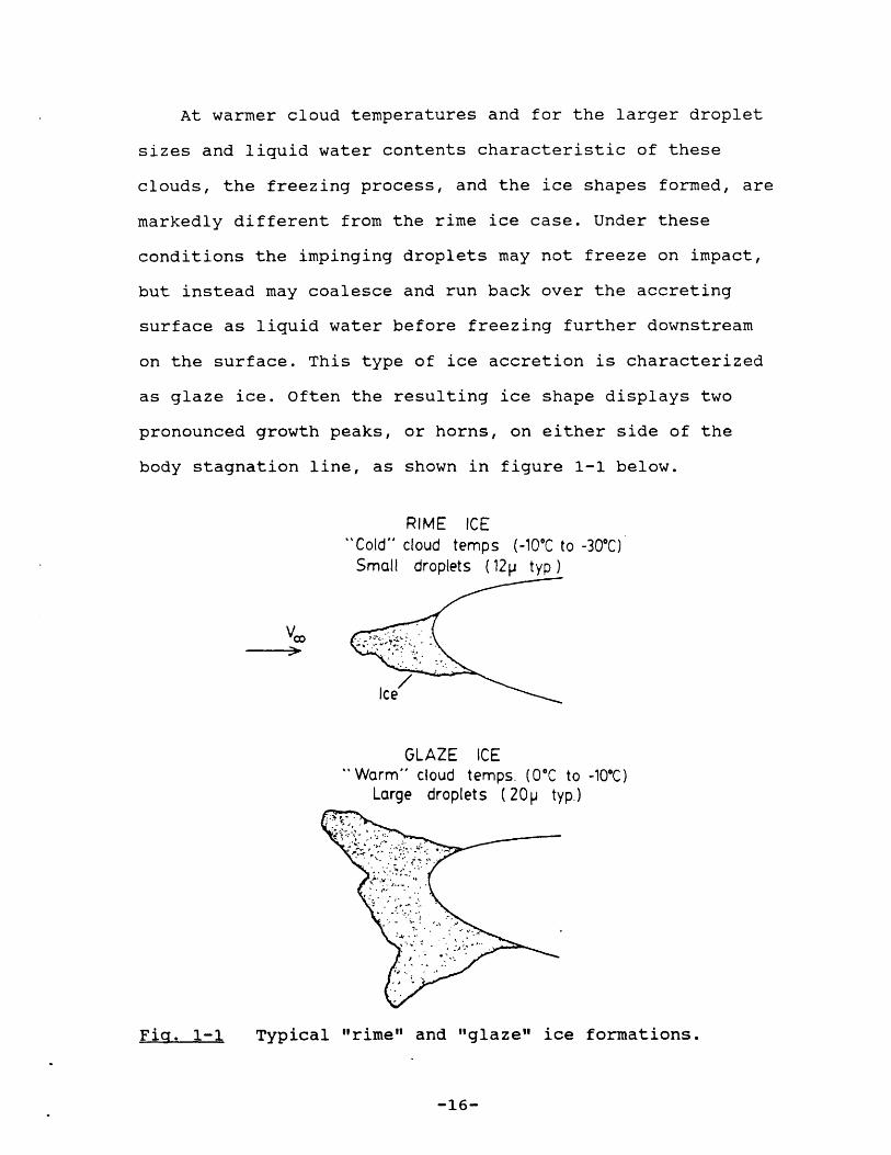
At warmer cloud temperatures and for the larger droplet

sizes and liquid water contents characteristic of these

clouds, the freezing process, and the ice shapes formed, are

markedly different from the rime ice case. Under these

conditions the impinging droplets may not freeze on impact,

but instead may coalesce and run back over the accreting

surface as liquid water before freezing further downstream

on the surface. This type of ice accretion is characterized

as glaze ice. Often the resulting ice shape displays two

pronounced growth peaks, or horns, on either side of the

body stagnation line, as shown in figure 1-1 below.

RIME ICE'Cold" cloud temps (-10 0C to -30*C)

Small droplets (12p typ)

Ice

GLAZE ICEWarm" cloud temps. (O'C to -10*C)

Large droplets (20p typ.)

Fig. 1-1 Typical "rime" and "glaze" ice formations.

-16-

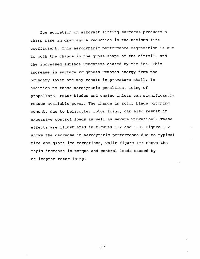
Ice accretion on aircraft lifting surfaces produces a

sharp rise in drag and a reduction in the maximum lift

coefficient. This aerodynamic performance degradation is due

to both the change in the gross shape of the airfoil, and

the increased surface roughness caused by the ice. This

increase in surface roughness removes energy from the

boundary layer and may result in premature stall. In

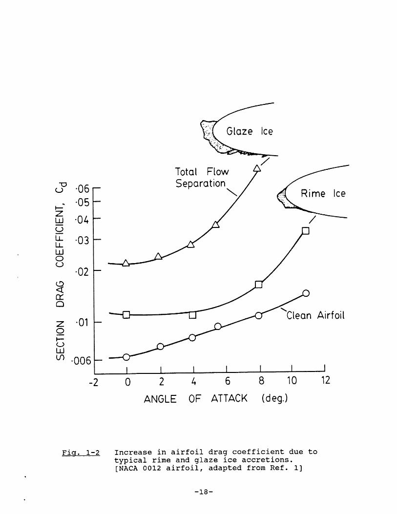
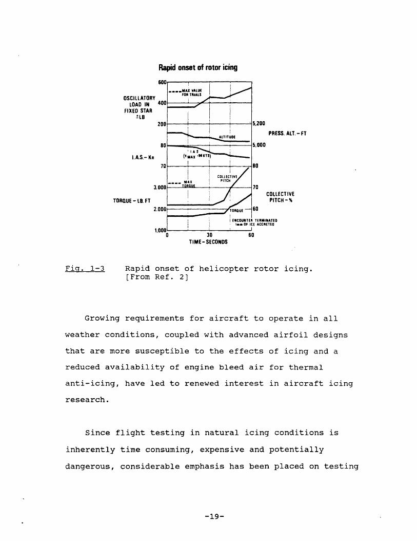
addition to these aerodynamic penalties, icing of

propellors, rotor blades and engine inlets can significantly

reduce available power. The change in rotor blade pitching

moment, due to helicopter rotor icing, can also result in

excessive control loads as well as severe vibration2 . These

effects are illustrated in figures 1-2 and 1-3. Figure 1-2

shows the decrease in aerodynamic performance due to typical

rime and glaze ice formations, while figure 1-3 shows the

rapid increase in torque and control loads caused by

helicopter rotor icing.

-17-

Total FlowSeparation

Rime Ice

Clean Airfoil

I II I I

8 10

ANGLE OF ATTACK

12

(deg.)

FiCg. 1-2 Increase in airfoil drag coefficient due totypical rime and glaze ice accretions.[NACA 0012 airfoil, adapted from Ref. 1]

-18-

C-)

U-1

0U-

z0

U0

-06-05

04

-03

-02

-01

-006I I I I- I -

Rapid onset of rotor icing

OSCILLATORYLOAD IN

FIXED STAR±LB

I. A.S.- Kn

3

TORQUE - LB. FT

PRESS. ALT. - FT

COLLECTIVEPITCH - %

30TIME- SECONDS

Fig. 1-3 Rapid onset of helicopter rotor icing.[From Ref. 2]

Growing requirements for aircraft to operate in all

weather conditions, coupled with advanced airfoil designs

that are more susceptible to the effects of icing and a

reduced availability of engine bleed air for thermal

anti-icing, have led to renewed interest in aircraft icing

research.

Since flight testing in natural icing conditions is

inherently time consuming, expensive and potentially

dangerous, considerable emphasis has been placed on testing

-19-

in icing wind tunnels. Due to facility limitations it is

often impossible to test full size aircraft components or to

duplicate the desired flight icing conditions; thus accurate

icing scaling laws need to be developed in order to

alleviate these limitations. Another area that has received

considerable attention is the development of computer codes

to predict ice accretion under different icing conditions.

If the geometry, location and roughness of the ice can be

determined then the aerodynamic performance of the iced

component can be calculated using appropriate CFD codes.

Fundamental to both the development of icing scaling laws

and computer codes to predict ice shapes is an accurate

physical model of the ice accretion process itself. Current

models used to describe the icing process are discussed in

the next section.

1.2 MODELING THE ICE ACCRETION PROCESS

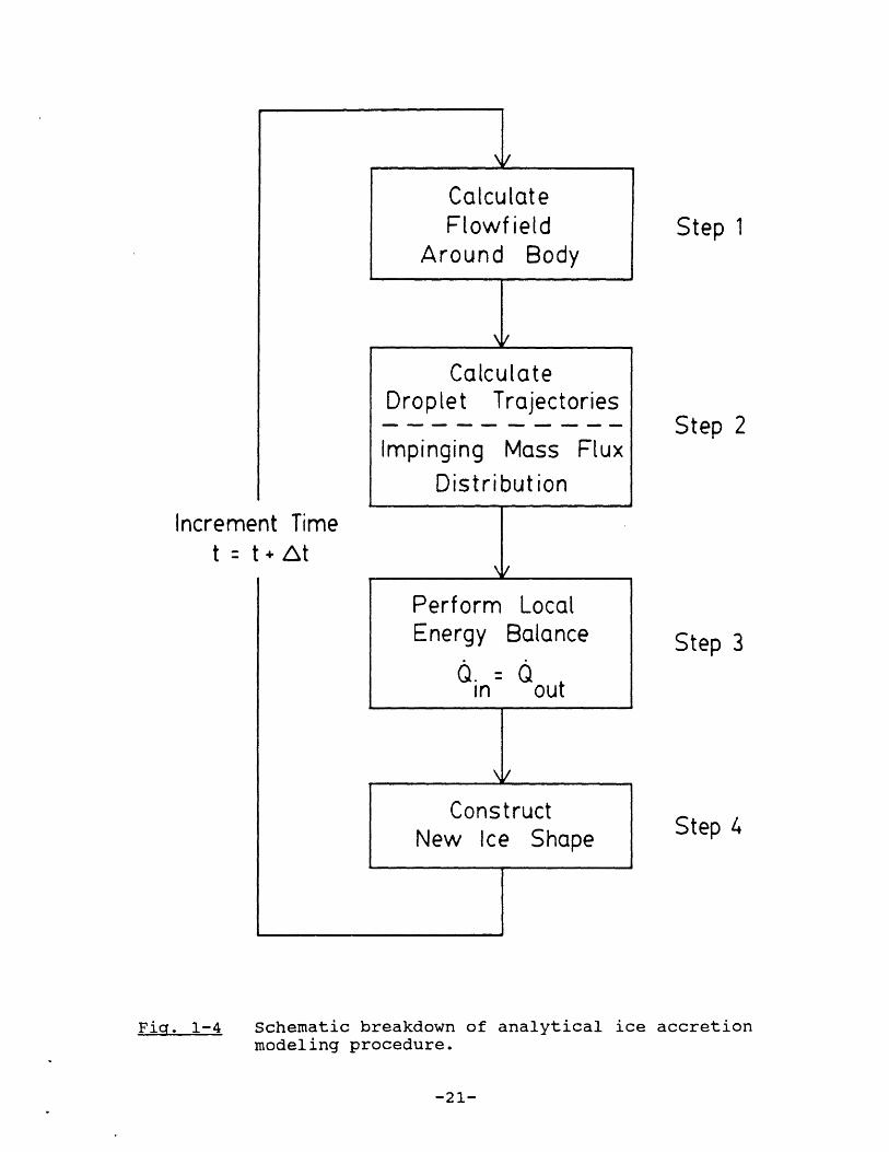
Figure 1-4 illustrates schematically how recent3-5

attempts to analytically model aircraft icing have

decomposed the ice accretion process. First, the aerodynamic

flowfield around the body of interest is calculated, usually

by a potential flow panelling method. Droplet trajectories

around the body are then calculated by integrating the

droplet equations of motion within the body flowfield.

-20-

increment Timet = t + t

\/

CalculateFlowfi eld

Around Body

\/Calculate

Droplet Trajectories

Impinging Mass FluxDistribution

Perform LocalEnergy Balance

Q. =Qin out

ConstructNew Ice Shape

Fig. 1-4 Schematic breakdownmodeling procedure.

of analytical ice accretion

-21-

Step 1

Step 2

Step 3

Step 4

From these trajectory calculations the impinging mass flux

distribution due to the droplets can then be determined

around the body.

The third, and crucial step, involves a thermodynamic

analysis of the freezing process at the icing surface.

Typically a steady-state energy balance is applied to a

series of small control volumes along the icing surface. For

each control volume the heat of fusion released as the

impinging droplets freeze is balanced by the rate at which

heat can be removed from the control volume. The final step

involves calculating the mass of ice formed at each location

on the body as a result of satisfying this energy balance,

and constructing the resulting ice shape. This entire

process may then be repeated using the iced geometry as

input for the flowfield calculation. Due to this form of

time-stepped solution, and the inherent feedback

relationship between the ice shape and flowfield, any errors

in each of these four steps tend to propagate and may result

in unrealistic ice shape predictions.

Experimental measurements6-8 have confirmed the accuracy

of the flowfield and droplet trajectory calculations. For

rime ice growth the droplets are assumed to freeze at the

point of impact, and thus no thermodynamic analysis is

necessary. In this case the ice shapes predicted are in good

-22-

agreement with experimentally measured ice growths3 , as

can be seen in Figure 1-5 below.

Experiment (IRT) Calculated (LEWICE)

Accreted Ice Shape After 2 Minutes Exposure

After 5 Minutes

Fic. 1-5 Comparison of experimentally measured airfoil iceaccretion and analytically predicted ice growth,for rime ice conditions. [From Ref. 3]

-23-

TEMP LWC MVD VEL('C) (g/m3) (p) (m/s)

-26-1 102 12 521

......................................

4-

However, for glaze ice conditions the ice shapes

predicted -using the local energy balance method are

extremely sensitive to the assumed convective heat transfer

distribution over the body3 ,9' 1 0 . Figure 1-6 illustrates

this sensitivity, and shows the variation in glaze ice

shapes predicted using different assumed surface roughness

heights for the heat transfer calculation. Due, at least in

part, to this sensitivity to the heat transfer distribution,

and the lack of experimental data in this area, an analytic

model capable of accurately predicting ice shapes throughout

the glaze icing regime has not yet been demonstrated.

-24-

Rime feathers

Experiment (IRT)

Roughness, ks = 0-5mm ks = 1-0mm

ks 20mm ks 40mm

Calculated (LEWICE)

Fig. 1-6 Effect of assumed surface roughness, ks, onanalytically predicted ice growth, for glaze iceconditions. [From Ref. 9]

-25-

TEMP LWC MVD VEL(*C) (g/m3) (P) (m/s)

-14-4 0-96 37-5 93-9

Chapter 2

STEADY-STATE THERMODYNAMIC ANALYSIS OF AN ICING

SURFACE

2.1 MODES OF ENERGY TRANSFER

The thermodynamic analysis presented here for a surface

accreting ice follows the steady-state energy balance

approach first proposed by Messinger1 l. Figure 2-1 shows the

modes of energy transfer associated with an icing surface.

Six different forms of energy transport are considered.

AerodynamicHea

Latent Heat

of Fusion icLeation ofI n D ts

DropletKineticEnergy

Sublimation /Evaporation

Fig. 2-1 Modes of energy transfer for an accreting icesurface.

-26-

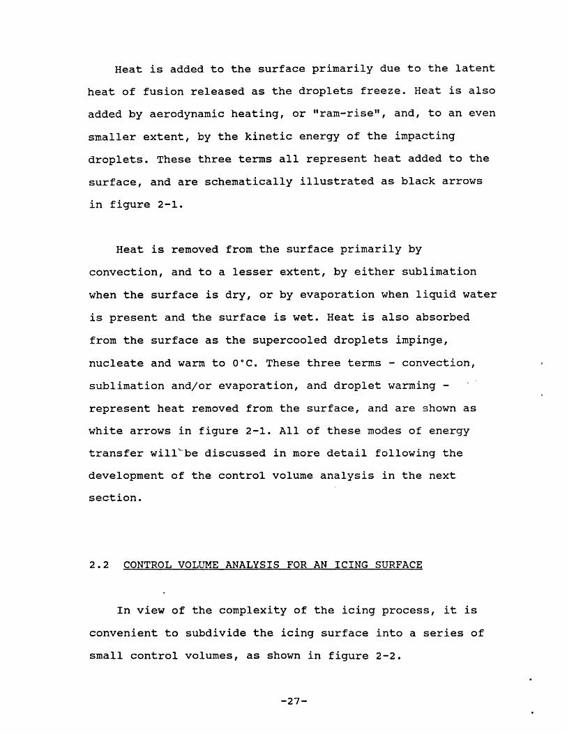
Heat is added to the surface primarily due to the latent

heat of fusion released as the droplets freeze. Heat is also

added by aerodynamic heating, or "ram-rise", and, to an even

smaller extent, by the kinetic energy of the impacting

droplets. These three terms all represent heat added to the

surface, and are schematically illustrated as black arrows

in figure 2-1.

Heat is removed from the surface primarily by

convection, and to a lesser extent, by either sublimation

when the surface is dry, or by evaporation when liquid water

is present and the surface is wet. Heat is also absorbed

from the surface as the supercooled droplets impinge,

nucleate and warm to O'C. These three terms - convection,

sublimation and/or evaporation, and droplet warming -

represent heat removed from the surface, and are shown as

white arrows in figure 2-1. All of these modes of energy

transfer will'be discussed in more detail following the

development of the control volume analysis in the next

section.

2.2 CONTROL VOLUME ANALYSIS FOR AN ICING SURFACE

In view of the complexity of the icing process, it is

convenient to subdivide the icing surface into a series of

small control volumes, as shown in figure 2-2.

-27-

Control Volumes

Accreting Body

VC

Ice < ,/

Fig. 2-2 Control Volume Definition.

If a sufficiently short time interval is considered, so

that the flowfield is not significantly altered by the ice

growth during that period, and if the ambient icing

conditions remain constant throughout the time interval,

then each control volume will experience quasi steady-state

icing conditions. This quasi steady-state assumption is

fundamental to the thermodynamic analysis presented here for

the icing surface and again is only valid when:

1. The ice growth during the time period considered does

not significantly alter the flowfield.

2. The ambient icing conditions do not vary significantly

over the time period considered.

3. The control volume is sufficiently small so that spatial

-28-

variations may be neglected.

The effects of unsteady ambient icing conditions,

frequently encountered in flight, are discussed in

Chapters 5 and 6. The mass and energy balances appropriate

to the quasi steady-state case are presented in the

following sections.

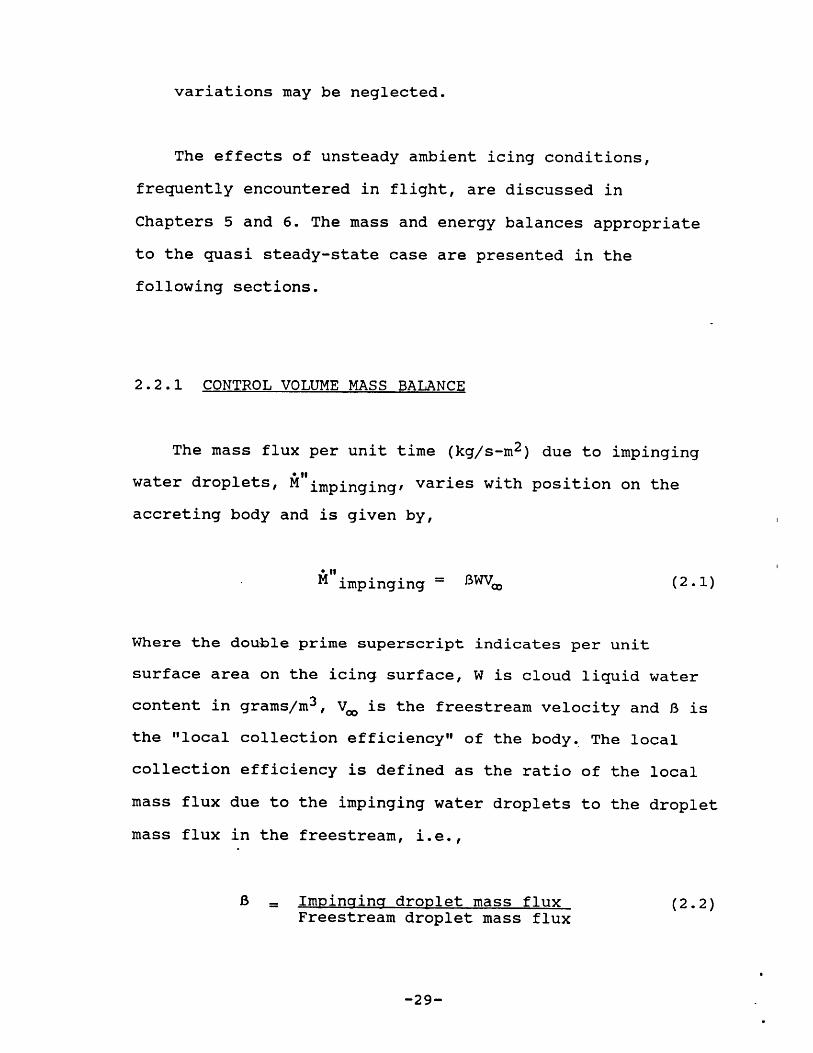
2.2.1 CONTROL VOLUME MASS BALANCE

The mass flux per unit time (kg/s-m2 ) due to impinging

water droplets, M"impinging, varies with position on the

accreting body and is given by,

Atimpinging = BWV, (2.1)

Where the double prime superscript indicates per unit

surface area on the icing surface, W is cloud liquid water

content in grams/m 3, V. is the freestream velocity and 8 is

the "local collection efficiency" of the body. The local

collection efficiency is defined as the ratio of the local

mass flux due to the impinging water droplets to the droplet

mass flux in the freestream, i.e.,

B = Impinging droplet mass flux (2.2)Freestream droplet mass flux

-29-

The local collection efficiency, B, is governed by the

ratio of the impinging droplets inertia to the aerodynamic

drag on them due to the freestream disturbance created by

the body. For most aircraft icing regimes the local

collection efficiency is primarily a function of the cloud

droplet size, characterized by the droplet median volume

diameter (MVD), and the size of the accreting body.

Figure 2-3 is a plot of the local collection efficiency

for a cylinder. The local collection efficiency is plotted

as a function of cylinder angle for several different cloud

droplet diameters. The local collection efficiency is a

maximum on the stagnation line (e = 0 *), and decreases with

increasing cylinder angle. Both the impingement area and the

local collection efficiency increase with droplet size, due

to the higher inertia of the droplets. In general then, a

small body moving rapidly through a cloud of large droplets

will have a much higher collection efficiency than a large

body moving slowly through a cloud of small droplets.

-30-

V = 10Om/s10cm dia..

,5 0p droplet diameter

10' 200 30 40 50 60' 70' 80 90

CYLINDER ANGLE,

Fig. 2-3 Local collection efficiency for a 10 cm diametercylinder, as a function of droplet size.

-31-

z

0--

-aJ

0

1-0

0-8

0-6

0-4

0-2

0-0

i) MASS BALANCE FOR DRY ICE GROWTH

When all the impinging droplets freeze on impact with

the accreting surface, the ice surface is "dry". Figure 2-4

schematically illustrates this condition. The control volume

mass balance equation is given by,

M ice = Miimpinging = BWV, (2.3)

Where again the double prime superscript indicates per unit

surface area of the icing surface. Equation 2.3 simply

states that the mass of ice formed per unit area per unit

time, A"ice' is equal to the local mass flux per unit time

due to the impinging droplets, N impinging- In this equation,

and throughout this analysis, the small contribution to the

mass balance due to sublimation (or evaporation in the case

of a wet ice surface) has been neglected.

The rate at which the local ice thickness, D, increases,

is referred to as the ice accretion rate, D. For dry ice

growth, the ice accretion rate is given by,

= ice/ ice = Bwvo/ ice (2.4)

Where 3ice is the density of the accreted ice.

-32-

wV0

~ '%1.~

-

Control Volume

D0 Mimpinging-

Droplets

Dry" ice surface

Fig. 2-4 Control volume mass balance for a dry icesurface.

-33-

ii) MASS BALANCE FOR WET ICE GROWTH

If the-rate at which heat can be removed from the icing

surface is insufficient to freeze all of the locally

impinging droplets, the ice surface will become wet, as

shown schematically in figure 2-5.

Liquid water on the ice surface will, in general, first.

appear in the stagnation region of the body, where the

impinging mass flux is a maximum. In this model, liquid

water formed on the icing surface is assumed to flow

downstream from the stagnation region, driven by the

external flowfield. This flow of liquid over the icing

surface is known as "run-back".

The control volume mass balance in the case of a wet ice

surface with run-back liquid present is thus,

Mice impinging + Mrun in - Mrun out (2.5)

Where Mrun in and Nrun out represent the mass flows (kg/sec)

into, and out of, the control volume due to run-back liquid

(see figure 2-5). The mass of liquid in the control volume,

Mwater, is taken to be constant, i.e. it is assumed in this

model that there is no accumulation of liquid in the control

volume in the steady-state. The mass flux per unit time of

droplets impinging on the local control volume, A"impinging'

-34-

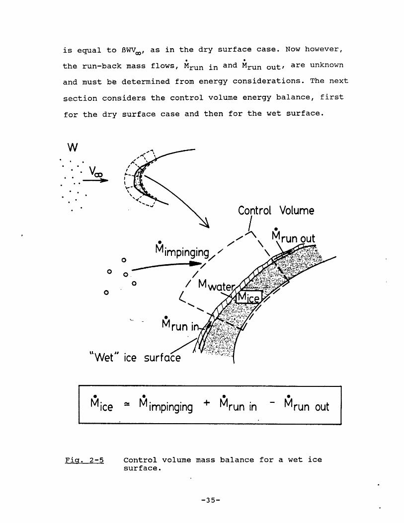
is equal to BWV,, as in the dry surface case. Now however,

the run-back mass flows, Mrun in and Mrun out' are unknown

and must be determined from energy considerations. The next

section considers the control volume energy balance, first

for the dry surface case and then for the wet surface.

W

rot Volume

MA

Mimpinging 7

0 o0 / Mwater

Mri inin -7

ttWet" ice sur

Fig. 2-5 Control volume mass balance for a wet icesurface.

-35-

2.2.2 CONTROL VOLUME ENERGY BALANCE

As discussed in section 2.1, six modes of energy

transfer to and from the icing surface are considered. The

steady-state assumption requires that the rate at which

energy is added to any control volume equals the rate at

which it is removed. Thus the fundamental energy equation

for the control volume is,

0iin = Q"out (2.6)

Where U"in and U"out respectively represent the energy added

to, and removed from, the control volume, per unit area per

unit time. Equation 2.6 may be expanded into its component

energy terms as,

Qin = Q freezing + 0"aero heating + 5"droplet k.e. (2.7)

out ~ conv + 0"subl + 0"droplet warming (2.8)

The ice surface is assumed to attain a steady-state,

locally uniform surface temperature, Tsurf- If the ice

surface is dry then the surface temperature must be less

than, or just equal to, 0*C. If the ice surface is wet the

surface temperature is assumed to be O'C. Steady-state

conduction into the icing surface is assumed to be zero, and

-36-

chordwise conduction between adjacent control volumes is

neglected.

i) ENERGY BALANCE FOR DRY ICE GROWTH

With these assumptions and definitions, equations 2.7

and 2.8 may be expanded for the dry ice surface case as,

freezing

aero heating

droplet k.e.

Q"convection

sublimation

droplet warming

A M imp[Lf + Ci(0*C - Tsurf)]

= hrV2/2Cp

impV2/2

= h(Tsurf - Too)

= hDwLs(v, surf - 3v,o)/k

A impCwATa,

Control volume energy transfer terms for a dry ice surface.

In these equations Tsurf is the equilibrium surface

temperature in degrees Centigrade and A"imp is the mass flux

-37-

(2.9)

(2.10)

(2.11)

(2.12)

(2.13)

(2.14)

per unit time of droplets impinging on the control volume,

BWV,. Using this expression for A"imp, and combining all the

above equations (2.9 - 2.14), yields the steady-state energy

balance equation for a dry ice surface,

BWVc[Lf + Ci(0"C - Tsurf) + V2/2] + hrV2/2Cp =

h[(Tsurf - To) + DwLs(?vsurf - ?v,o)/k] + BWVOCw TO

(2.15)

Steady-state energy balance equation for a dry ice surface.

ii) ENERGY BALANCE FOR WET ICE GROWTH

In considering the energy balance for the wet surface

case, it is convenient to define a quantity n, the "freezing

fraction" as,

n ' Mice (2.16)

Mimp + Mrun in

The freezing fraction is thus the ratio of the mass of ice

formed per unit time to the total mass of water entering the

control volume, per unit time.

When the ice surface is dry the freezing fraction is

always unity since Mice = Mimpand Mrun in is zero since no

-38-

liquid is present on the ice surface. For a wet ice surface

the freezing fraction must lie -between zero and unity. For

simplicity only the stagnation region energy balance will be

considered for the wet surface case.

iii) STAGNATION REGION ENERGY BALANCE FOR WET ICE GROWTH

Freestream

o.

Mout (Wet growth only)

Tsurf

0

Fig. 2-6 Stagnation region control volume.

Figure 2-6 depicts the stagnation region control volume

examined fQr the wet surface case. Since only the stagnation

region is considered, the only liquid entering the control

volume is due to impinging droplets, and no liquid runs into

the control volume, i.e. Mrun in = 0. From equation 2.16,

-39-

the freezing fraction, n, is thus simply,

n = Mice/Mimp (2.17)

Although no liquid runs into the stagnation region, liquid

may flow out of the control volume along the ice surface.

Using the mass balance equation (2.5) for the wet surface,

equation 2.17 may thus be written as,

n = Mimp - Mrun out = 1 - Mrun out (2.18)

Mimp Mimp

For the wet surface, the energy balance is altered from

the dry surface case in the following ways. The rate at

which ice is formed, per unit surface area, A"ice, is

reduced from the dry rate, M"imp = BWVc, to,

M ice = nM imp = nBWV. (2.19)

The ice accretion rate, D, for the wet surface is thus,

D = M ice/3ice = nBWV,/ 3ice (2.20)

-40-

The heat flux per unit time due to freezing, Q"freezing,

can be obtained from equations 2.9 and 2.19 as,

Q"freezing - A"ice[Lf + Ci(O0*C - Tsurf)] [2.9]

= nBWVLf (2.21)

Where Lf is the latent heat of fusion for water. Note that

the equilibrium temperature, Tsurf, for the wet surface is

assumed to be O'C, and thus there is no subsequent cooling

of the accreted ice.

In addition, evaporation, rather than sublimation, now

removes heat from the ice surface, and hence the latent heat

of vaporization ,Lv, is used in the- energy balance equation,

evap = hDwLv(3v,surf - 3v,D)/k (2.22)

The four remaining energy transport terms in the energy

balance - aerodynamic heating, droplet kinetic energy,

convection, and droplet warming (nucleation) - are unchanged

in the wet surface formulation. However, since the surface

temperature, Tsurf, is now assumed to be 0"C, both the

convective.and evaporative heat loss terms are evaluated for

a surface at O'C. With this, the energy balance equation for

the wet surface may be written as,

-41-

freezing + droplet k.e. + Q aero heating =

Q conv + Q evap + 6 droplet warming (2.23)

BWV,[nLf + V2/2] + hrV2/2Cp =

h[(0"C - Tc,) + DwLv(gyO*C - 3v,o,)/k] + BWVCW T0,

(2.24)

Stagnation region energy balance equation for a wet ice

surface.

iv) THRESHOLD CONDITION FOR TRANSITION FROM DRY TO WET ICE

SURFACE IN STAGNATION REGION

Of particular interest is the condition for which the

ice surface transitions from dry to wet. For the stagnation

region control volume considered above, this transition must

occur when the equilibrium surface temperature is 00C and

the freezing fraction is very slightly less than unity. For

this case, the stagnation region energy balance equation

(2.24) may be rearranged to yield a "critical impinging

liquid water content", (BW)crit, given by,

(BW)crit = h[(0*C - To) + DWLy(y,0*C - iv,o,)/k - rV2/2Cp]

Vo[Lf + V./2 - CwAT.)

(2.25)

-42-

For this limiting case between dry and wet growth, the

freezing fraction has been taken to be unity. Equation 2.25

states that, for a given freestream airspeed, ambient

temperature and local heat transfer coefficient, there

exists a critical "effective" cloud liquid water content

above which the icing surface will become wet. This

effective liquid water content is the product of the local.

collection efficiency of the surface and the cloud liquid

water content. Since the local collection efficiency is a

strong function of the cloud droplet size, this parameter,

(BW)crit, may be regarded as primarily an icing cloud

property.

From equation 2.25 it can be seen that the value of BW

at which transition between wet and dry ice growth occurs

depends on the magnitude of the local heat transfer

coefficient, h.-It should, therefore, be possible to obtain

the local heat transfer coefficient over an icing surface by

carefully measuring the impinging liquid water content for

which the surface just becomes wet.

The approach taken in this thesis is to compare

experimenta.lly observed cases of wet and dry ice growth with

the regimes of wet and and dry ice growth predicted by a

series of heat transfer coefficient models. This comparison

of different physical heat transfer models (rough or smooth

-43-

surface, for example), enables the actual heat transfer

processes occuring during natural and artificial icing

conditions'to be better understood and modeled.

2.3 COMPARISON OF HEAT TRANSFER MODELS

In order to compare different heat transfer coefficient

models is convenient to express the local heat transfer

coefficient, h, in terms of the non-dimensional Nusselt

number, Nu, where,

Nu = h d/k (2.26)

With d being the uniced diameter (or characteristic

dimension) of the body, and k the thermal conductivity of

air. It is common to model heat transfer coefficients in the

form of a power law relationship between the Nusselt number

and the Reynolds number, Re, as,

Nu = A ReB = A (3Vd/pc) B (2.27)

Where A and. B are experimentally derived constants.

Using these relationships for the heat transfer

coefficient (eqs. 2.26 & 2.27), allows the steady-state

-44-

energy balance equation for transition between wet and dry

ice growth (eq. 2.25), to be rewritten as,

(BW)crit = A k ( /plB (Vd)B-1 (T*/L*) (2.28)

Where (BW)crit is the critical impinging liquid water

content, above which the ice surface is expected to be wet.

The constants A and B represent the convective heat transfer

coefficient "model", or power law. The terms T* and L*

introduced in equation 2.28 are defined below as,

T* = [(O"C - Tc,) + DwLv(v,O*C - iv,o)/k - rV2/2Cp] (2.29)

L* = [Lf + V2/2 - CwnST,] (2.30)

The term T* can be thought of as representing the

effective temperature difference (in *C) between the icing

surface and the-freestream. This effective temperature

difference thus controls the rate at which heat is removed

from the icing surface by convection and evaporation. The

effect of aerodynamic heating is also included in this

temperature difference term.

In a similar way, the term L* represents an effective

heat of fusion (in J/Kg) "released" during the accretion

process. This term combines the latent heat of fusion of

water, Lf, the droplet specific kinetic energy, V2/2, and

-45-

the effective heat absorbed due to droplet warming on

impact, Cw&T,. Since the droplet kinetic energy and droplet

warming terms are typically an order of magnitude smaller

than the latent heat of fusion of water, the parameter L*

is, in most cases, essentially equal to Lf.

Equation 2.28 thus represents the wet/dry threshold for

the stagnation region of a body, predicted by the

steady-state energy balance analysis. If the impinging

liquid water content is less than the value of (BW)crit in

equation 2.28, then the ice surface is predicted to be dry;

while if BW is greater than (W)crit then the ice surface is

expected to be wet.

From this equation it can be seen that (BW)crit depends

on the assumed values of A and B in the heat transfer

coefficient model. By measuring the locally impinging liquid

water content, 8W, and whether the resulting ice surface is

wet or dry, it is thus possible to compare different heat

transfer models and determine which physical model best

predicts the observed wet or dry ice growth. The ultrasonic

pulse-echo techniques used to perform these experimental

measurements of ice accretion rate and ice surface condition

are described in the next chapter.

-46-

Chapter 3

REAL-TIME MEASUREMENT OF ICE GROWTH

USING

ULTRASONIC PULSE-ECHO TECHNIQUES

3.1 ULTRASONIC PULSE-ECHO THICKNESS MEASUREMENT

Figure 3-1 illustrates the principle of ultrasonic

pulse-echo thickness measurement for an icing surface. A

small transducer mounted flush with the accreting surface

emits a brief compressional wave, the ultrasonic "pulse",

that travels through the ice as shown. Typical transducer

frequencies used to generate the compressive wave are

between 1 and 5 MHz. This pulse is reflected at the ice

surface and returns to the emitting transducer as an echo

signal. By measuring the -time elapsed between the emission

of the pulse and the return of the echo, Tp-e, the ice

thickness over the transducer, D, may be calculated from the

formula,

D = C Tp.e/2 (3.1)

Where C is the speed of propagation of the compressional

wave in ice.

-47-

AIR

PULSE PULSE 2nd RETURN[

EMITTED

1st ICE /AIR ECHO RETURNI

ULTRASONIC TRANSOUCE

D

LSE 1st ICE/AIRITTED ECHO RETURN

1

R SURFACE

2nd RETURN 3rd RETURN

T -- ATTENUATION

TIME (pS)

Tp-e--

-- Tp-e--4

Ficg. 3-1 Ultrasonic pulse-echo thickness measurement andtypical ultrasonic pulse-echo signal in ice.

-48-

C-Tp-e

2

PUEM

f I

11

This speed of propagation has been shown (see Appendix

A) to be insensitive to the different types of ice (glaze,

rime and mixed) accreted at typical flight airspeeds; a

value of 3.8mm/psec has been used for all the results

presented in this thesis. Experimental measurements of the

variation in the speed of sound for different ice formations

are contained in Appendix A, along with a more detailed

discussion of the ultrasonic pulse-echo technique.

Figure 3-1 also shows a typical ultrasonic pulse-echo

signal obtained from a stationary, i.e. non-accreting, ice

surface. As indicated in the figure, the time elapsed

between the emission of the pulse and the return of the echo

from the ice surface is on the order of microseconds for the

ice thicknesses of concern for aircraft icing (lmm-20mm). By

repeatedly emitting pulses, the ice thickness can be

constantly measured as ice accretes on the body. Pulses are

typically emitted several thousand times a second, and hence

essentially "real-time" measurement of the ice thickness is

possible. In addition to obtaining the ice thickness from

the pulse-echo transit time, the presence or absence of

liquid water on the ice surface may be detected from the

characteristics of the received echo signal. These signal

characteristics are discussed in the next two sections.

-49-

3.2 ULTRASONIC SIGNAL CHARACTERISTICS FOR DRY ICE GROWTH

If all the droplets impinging at a given location on a

body freeze on impact, the freezing fraction is unity and

the ice surface formed will be "dry", as discussed in

Chapter 2. This form of ice accretion will be referred to as

dry ice growth, and is characteristic of rime ice formations

at low temperatures.

Figure 3-2 illustrates the behaviour of the ultrasonic

echo signal received during dry ice growth. The echo

waveform simply translates in time as the ice thickness, and

hence pulse-echo time, increase. The rate at which the echo

signal translates is thus proportional to the ice accretion

rate. This simple translation of the echo waveform is a

result of the extremely brief time taken for the impinging

droplets to freeze. The ice surface formed under these

conditions is relatively ~smooth, and thus a well-defined

echo waveform with a narrow echo width is typically

received, as indicated in the figure.

-50-

TIME t1

AIR

-ICE/AIR ECHO[I E/ I

TIME f2

AIR

--

02

ICE/AIR ECHOj

SURFACEULTRASONIC TRANSDUCER

t2 ) t1 02 ) 01

ICE/AIR ECHOAT 1

23 ItIt

1 2 3 4

Tp-e

ICE/AIR ECHOAT 2

i i

5 6TIME (p S)

Tp-e 2

Fig. 3-2 Ultrasonic signal characteristics fordry ice growth.

-51-

F01

PULSE EMITTED

1 3I

3.3 ULTRASONIC SIGNAL CHARACTERISTICS FOR WET ICE GROWTH

If the heat transfer from the accreting surface is

insufficient to completely freeze all the impinging

droplets, the freezing fraction is less than unity and

liquid water will be present on the ice surface. This form

of ice accretion will be referred to as wet ice growth, and

is characteristic of glaze and mixed ice formation at

ambient temperatures just below 0*C.

During wet ice growth the ice surface is covered, at

least partially, by a thin liquid layer. The emitted

ultrasonic pulse thus encounters two separate interfaces, as

shown in figure 3-3. The first interface encountered by the

outgoing pulse is that between the ice and the water lying

on the ice su'rface. This interface will be referred to as

the ice/water interface. The other interface encountered is

that between the liquid water and the ambient air, the

water/air interface. Two echo signals are therefore

received; the first from the ice/water interface, and a

second, later echo from the water/air interface.

The first echoes received (labelled "A" to "B" in

figure 3-3), are from the ice/water interface, and have a

characteristically broader echo width than that received

-52-

AIR

WATER

o MULTIPLE WATER/AIR ECHOESI

-CE/ATER ECHO .

ULTRASONIC

PULSE EMITTED

TRANSDUCER

ICE/WATER ECHOES,SLOW VARIATION

STATIONARY

A BMULTIPLE WATER/AIR ECHOES,

RAPID VARIATION

TIME (pS)

Tp-e

Fig. 3-3 Ultrasonic signal characteristicswet ice growth.

-53-

SURN-ALE

for

;00,zx/x,0 00

during rime, or dry, ice growth. This broad echo width is

due to the rougher ice surface characteristic of glaze, or

wet, ice growth.

The rougher ice surface typically observed during wet

ice growth is illustrated in figure 3-3. The variations in

ice thickness (exaggerated for clarity), over the area of

the transducer* increase the width of the received echo. The

start of the echo return from the ice surface, labelled "A"

in figure 3-3, represents the minimum ice thickness over the

transducer. The last echo return from the ice surface,

labelled "B", corresponds to the maximum ice thickness over

the transducer. The central region of the ice surface echo,

"C", was used as representative of the average local ice

thickness for all the test results presented.

As in the dry growth case, these ice/water echoes

translate in time as liquid freezes at the interface and the

ice thickness increases. Now however, the freezing process

is no longer "instantaneous", and the detailed shape of the

ice/water echoes slowly varies as liquid freezes over the

transducer.

*The ultrasonic transducers used typically had diameters of

approximately 0.65 or 1.30 cm.

-54-

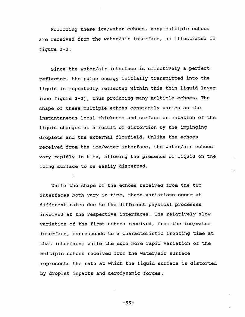
Following these ice/water echoes, many multiple echoes

are received from the water/air interface, as illustrated in

figure 3-3-.

Since the water/air interface is effectively a perfect,

reflector, the pulse energy initially transmitted into the

liquid is repeatedly reflected within this thin liquid layer

(see figure 3-3), thus producing many multiple echoes. The

shape of these multiple echoes constantly varies as the

instantaneous local thickness and surface orientation of the

liquid changes as a result of distortion by the impinging

droplets and the external flowfield. Unlike the echoes

received from the ice/water interface, the water/air echoes

vary rapidly in time, allowing the presence of liquid on the

icing surface to be easily discerned.

While the shape of the echoes received from the two

interfaces both-vary in time, these variations occur at

different rates due to the different physical processes

involved at the respective interfaces. The relatively slow

variation of the first echoes received, from the ice/water

interface, corresponds to a characteristic freezing time at

that interface; while the much more rapid variation of the

multiple echoes received from the water/air surface

represents the rate at which the liquid surface is distorted

by droplet impacts and aerodynamic forces.

-55-

3.4 SUMMARY

Ultrasonic pulse-echo techniques can be used to

accurately and continuously measure ice thickness on an

accreting surface. During wet ice growth, liquid on the ice

surface produces a constantly distorting, reflective

interface for the emitted ultrasonic pulse. As a result, the

echoes received during wet growth display a rapid time

variation that is absent when the ice surface is dry. Hence

by examining the time variation of the echo signals

received, the presence or absence of liquid on the ice

surface may be clearly discerned.

-56-

Chapter 4

ICING OF A CYLINDER DURING ARTIFICIAL ICING CONDITIONS

4.1 OVERVIEW

This chapter describes experimental measurements of ice

growth on a cylinder exposed to artificial icing conditions

produced in the NASA Lewis Icing Research Tunnel. Ice

thickness and surface condition (wet or dry) were measured

for a variety of icing cloud conditions, using ultrasonic

pulse-echo techniques. Sections 4.2 and 4.3 describe the

experimental apparatus used and the cylinder installation

and test procedure in the icing wind tunnel. Section 4.4

presents experimental results for different icing cloud

conditions. Results are presented in the form of ice

thickness versus icing time and ice accretion rate versus

cloud temperature. The effects of exposure time and cloud

temperature are compared and discussed. Ice accretion rates

measured during wet and dry ice growth are used to infer

freezing fractions for the stagnation region, and to examine

liquid runback along the ice surface.

In Section 4.5, the ultrasonically measured wet or dry

ice surface conditions and corresponding accretion rates are

used to compare a series of assumed heat transfer

-57-

coefficients for the icing surface. The heat transfer

coefficients used are the experimental measurements of Van

Fossen et al., for a cylinder with a known surface roughness

exposed to crossflow at different freestream turbulence

levels1 2 . Results are presented in the form of wet/dry

"threshold" curves for each heat transfer model, plotted

together with experimentally observed wet and dry ice growth

cases. Section 4.6 summarizes the important features of the

experimentally observed ice growth behaviour in the Icing

Research Tunnel. Conclusions about the heat transfer

magnitude over the icing surface, based on the analysis in

Section 4.5, are also presented.

4.2 EXPERIMENTAL APPARATUS

Figure 4-1 illustrates schematically the apparatus and

experimental -Configuration used for these tests. The

equipment employed consisted of four main components, listed

below.

(1) A cylinder instrumented with small ultrasonic

transducers flush with the cylinder surface.

(2) A pulser/receiver unit to drive the transducers.

(3) An oscilloscope to display the pulse-echo signal.

-58-

60 MHz BANDWIDTH, DUAL CHANNEL OSCILLOSCOPE

VIDEO CAMERA

TO VIDEO RECORDER

ICING CLOUD

Fig. 4-1

-I~~'a

- CYLINDER

ULTRASONIC TRANSDUCERSFLUSH WITH CYLINDERSURFACE

Schematic of experimental apparatusconfiguration.

-59-

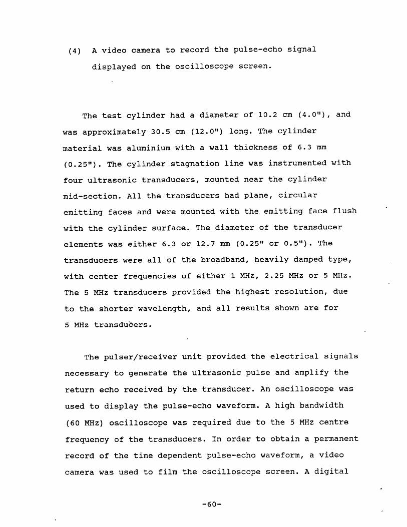
(4) A video camera to record the pulse-echo signal

displayed on the oscilloscope screen.

The test cylinder had a diameter of 10.2 cm (4.0"), and

was approximately 30.5 cm (12.0") long. The cylinder

material was aluminium with a wall thickness of 6.3 mm

(0.25"). The cylinder stagnation line was instrumented with

four ultrasonic transducers, mounted near the cylinder

mid-section. All the transducers had plane, circular

emitting faces and were mounted with the emitting face flush

with the cylinder surface. The diameter of the transducer

elements was either 6.3 or 12.7 mm (0.25" or 0.5"). The

transducers were all of the broadband, heavily damped type,

with center frequencies of either 1 MHz, 2.25 MHz or 5 MHz.

The 5 MHz transducers provided the highest resolution, due

to the shorter wavelength, and all results shown are for

5 MHz transducers.

The pulser/receiver unit provided the electrical signals

necessary to generate the ultrasonic pulse and amplify the

return echo received by the transducer. An oscilloscope was

used to display the pulse-echo waveform. A high bandwidth

(60 MHz) oscilloscope was required due to the 5 MHz centre

frequency of the transducers. In order to obtain a permanent

record of the time dependent pulse-echo waveform, a video

camera was used to film the oscilloscope screen. A digital

-60-

clock within the camera's field of view allowed the cylinder

exposure time to be simultaneously recorded.

4.3 ICING RESEARCH TUNNEL INSTALLATION AND TEST PROCEDURE

4.3.1 THE ICING RESEARCH TUNNEL

The icing wind tunnel used was the NASA Lewis Research

Center's Icing Research Tunnel (IRT). The Icing Research

Tunnel is a closed loop, refrigerated wind tunnel capable of

generating airspeeds up to 134 m/s (300mph) over a test

section area 1.83 m high and 2.74 m wide (6' x 9'). A large

refrigeration plant allows total air temperatures as low as

-340C to be achieved. A spray bar system upstream of the

test section 'is-used to produce the icing cloud. The cloud

liquid water content can be varied from 0.3 to 3.0 g/m3 and

the droplet median volume diameter from 10 to 40 microns.

Although the icing cloud fills the entire test section,

the cloud liquid water content varies over the test section

area. A central region of nearly constant liquid water

content exists, and is referred to as the "calibrated cloud"

(see figure 4-2). The calibrated cloud region is

approximately 0.6 m (2') high and 1.5 m (5') wide. The

-61-

EXTENSION POST-

TEST CYLINDER-12" x 4"Dia.

ICING RESEARCH

ICING CLOUD

SIDE VIEW

TUNNEL (IRT)

1~~~....

FRONT VIEW

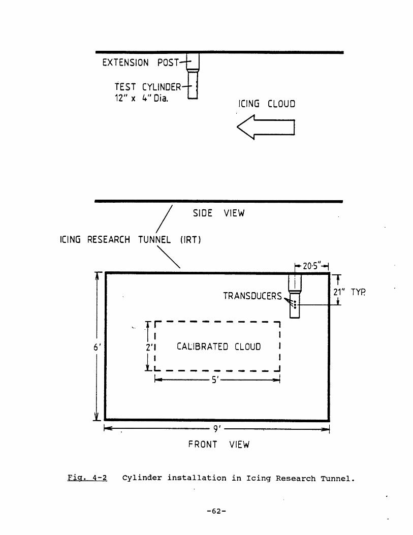
Fig. 4-2 Cylinder installation in Icing Research Tunnel.

-62-

TYP

liquid water content outside this region decreases, and is

near zero close to the tunnel walls.

4.3.2 CYLINDER INSTALLATION

The test cylinder installation in the Icing Research

Tunnel is shown in figures 4-2 and 4-3. The cylinder was

suspended vertically on an extension post mounted in the

roof of the IRT. However, in order to allow another

experiment unobstructed access to the icing cloud, the

cylinder did not fully extend into the calibrated region of

the icing cloud. As a result, the liquid water content at

the cylinder location was lower than that in the calibrated

region. The freestream velocity, temperature, and droplet

size distribution at the cylinder location were assumed to

be equal to the calibrated region values1 3 . Figure 4-3 is a

photograph of'the cylinder installation in the IRT test

section, looking upstream-. The test cylinder is in the top

left hand corner of the photograph. The airfoil in the

centre of the photograph occupies the calibrated region of

the icing cloud, produced by the spray bar system visible in

the background.

-63-

Fig. 4-3 Photograph of cylinder installation in IRT test

section (looking upstream).

4.3.3 TEST PROCEDURE

The test procedure for each different icing condition

simulated was as follows. With the water spray off, and the

test section airspeed set, the tunnel temperature was

lowered to the desired value. Once the tunnel temperature

had stabilized, the water spray system was turned on in

order to produce the icing cloud. The cloud liquid water

content and median volume diameter were set by the spray bar

-64-

water flow rate and injection pressures.

The pulse-echo signals from the transducers mounted in

the cylinder were recorded by the video camera as ice

accreted on the cylinder. Typically the spray system was

activated for a six minute period, after which it was turned

off. Constant icing conditions were maintained throughout

each exposure, or run. At the completion of each run, the

iced diameter of the cylinder was measured at each

transducer location, using a pair of outside calipers. The

ice thickness over the transducers was inferred from this

"mechanical" measurement. The cylinder was then completely

de-iced in preparation for the next run.

4.3.4 TEST ICING CONDITIONS

Ice growth was measured using the ultrasonic pulse-echo

technique for fifteen different icing cloud conditions,

ranging from glaze to rime icing conditions. Table 4-1 lists

the range of icing cloud characteristics for these tests.

-65-

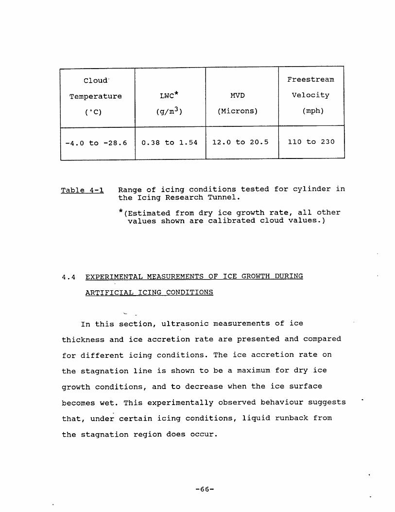
Table 4-1 Range of icing conditions tested for cylinder inthe Icing Research Tunnel.

(Estimated from dry ice growth rate, all othervalues shown are calibrated cloud values.)

4.4 EXPERIMENTAL MEASUREMENTS OF ICE GROWTH DURING

ARTIFICIAL ICING CONDITIONS

In this section, ultrasonic measurements of ice

thickness and ice accretion rate are presented and compared

for different icing conditions. The ice accretion rate on

the stagnation line is shown to be a maximum for dry ice

growth conditions, and to decrease when the ice surface

becomes wet. This experimentally observed behaviour suggests

that, under certain icing conditions, liquid runback from

the stagnation region does occur.

-66-

Cloud- Freestream

Temperature LWC* MVD Velocity

(0C) (g/m3) (Microns) (mph)

-4.0 to -28.6 0.38 to 1.54 12.0 to 20.5 110 to 230

4.4.1 COMPARISON OF ICE GROWTH DURING HEAVY AND LIGHT ICING

CONDITIONS

Figures 4-4 and 4-5 are plots of ice thickness, measured

with the ultrasonic system, versus exposure time. Ice growth

is shown at three different icing cloud temperatures for

"heavy" and "light" icing conditions.

The heavy icing conditions (figure 4-4) represent an

icing cloud with a high liquid water content, 0.77 g/m3 , and

a relatively large median volume drop diameter of 20

microns. The light icing conditions (figure 4-5) represent

an icing cloud with a lower liquid water content and smaller

droplet size. The liquid water content for the light icing

conditions, 0.38 g/m3 , is half the heavy icing value, and

the median volume drop diameter is reduced from 20 microns

to 12 microns. The freestream velocity is 103 m/s (230mph)

for both the heavy and light icing conditions.

Since the test cylinder was located outside the

calibrated cloud (see Section 4.3), the values given for the

icing cloud conditions are approximate. In particular, the

liquid water content at the cylinder location was estimated

to be 64% of the calibrated cloud value. This estimate is

based on the cylinder ice accretion rates measured for dry

ice growth; the experimental data used to derive this

corrected liquid water content is contained in Appendix B.

-67-

MECHANICALLY MEASUREDICE THICKNESS----- (*

TC= -28-6'C6 = 3-15mm/minRIME, DRY T.=- 17-5'C

O = 2-10mm/minGLAZE, WET

T =-8-0'CO = 0-75mm/minGLAZE, WET

1 2 3 4

EXPOSURE

Fig. 4-4

TIME (MINUTES)

Ice growth measured for "heavy" icing conditions.

-68-

TUNNEL CONDITIONSLWC G/M3 - 0-77MVO p -20VEL MPH - 230

LUzL.j

LU

MECHANICALLY MEICE THICKNESS

-28 6'CO = 1-05mm/minRIME, DRY

ASURED

T0O= -17-5'C0 = 1-05mm/minMIXED, DRY

T =-80O'CO=55mm/min

GLAZE, WET

1 2 3 4 5

EXPOSURE

Ficg. 4-5

TIME (MINUTES)

Ice growth measured for "light" icing conditions.

-69-

TUNNEL CONDITIONSLWC G/M3 ~0-38MVD p -12VEL MPH -230

4-

3

2

1 -

00

TC, =

As stated earlier, the freestream velocity, cloud

temperature and droplet size distribution for the cylinder

location were assumed to be approximately equal to the

calibrated cloud values.

Figures 4-4 and 4-5 show the ultrasonically measured ice

growth on the cylinder stagnation line for three different

cloud temperatures, -8.0*C, -17.5 0C and -28.6*C. The type of

ice growth occurring, wet or dry, is also indicated for each

exposure. The ultrasonic echo characteristics from the

accreting ice surface were used to determine if the growth

was wet or dry, as explained in Chapter 3. The caliper

measured ice thickness at the completion of each exposure is

also shown, if known. These mechanical measurements are seen

to be in close agreement (±0.5 mm) with the ultrasonically

measured thicknesses, and confirm the accuracy of the

pulse-echo measurement technique. The important features of

the ice growth behaviour for the heavy and light icing

conditions shown are discussed below.

i) EFFECT OF EXPOSURE TIME ON ICING RATE

The ice. growth plots in figures 4-4 and 4-5 all show a

relatively linear increase in ice thickness with exposure

time; the ice accretion rate, given by the slope of the ice

thickness curve, is therefore approximately constant

-70-

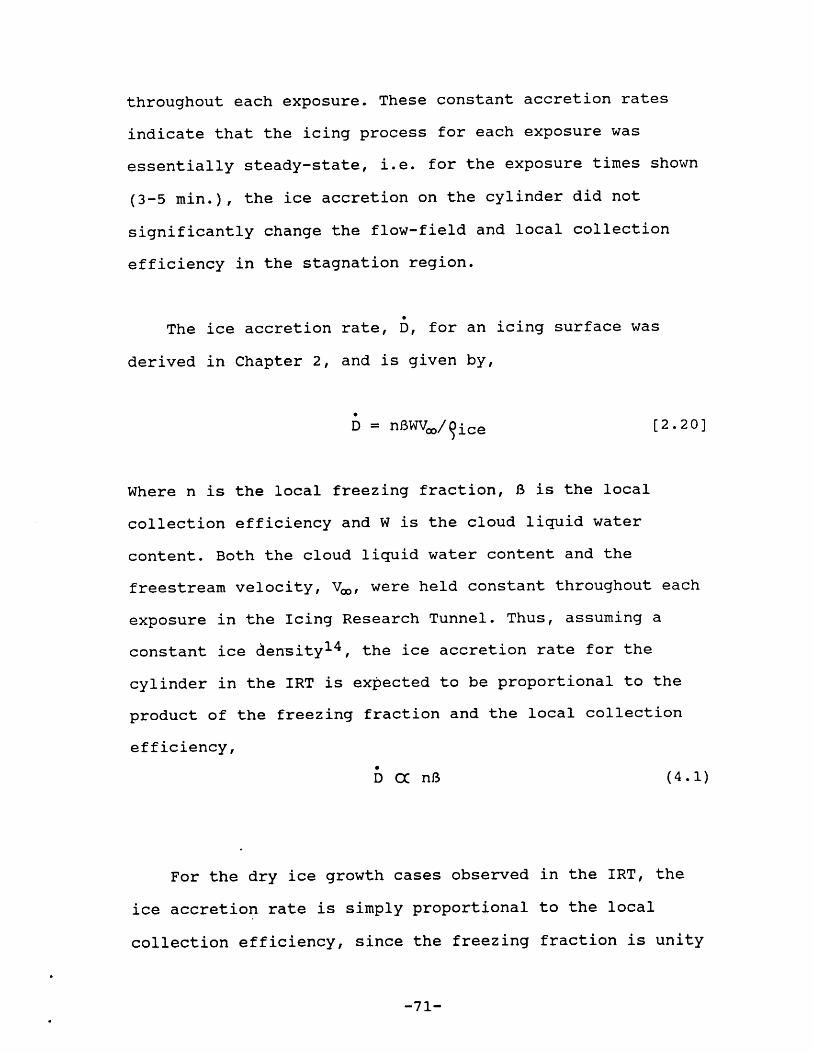
throughout each exposure. These constant accretion rates

indicate that the icing process for each exposure was

essentially steady-state, i.e. for the exposure times shown

(3-5 min.), the ice accretion on the cylinder did not

significantly change the flow-field and local collection

efficiency in the stagnation region.

The ice accretion rate, D, for an icing surface was

derived in Chapter 2, and is given by,

D = nBWVe/ ice [2.20]

Where n is the local freezing fraction, B is the local

collection efficiency and W is the cloud liquid water

content. Both the cloud liquid water content and the

freestream velocity, V, were held constant throughout each

exposure in the Icing Research Tunnel. Thus, assuming a

constant ice density14 , the ice accretion rate for the

cylinder in the IRT is expected to be proportional to the

product of the freezing fraction and the local collection

efficiency,

D C nB (4.1)

For the dry ice growth cases observed in the IRT, the

ice accretion rate is simply proportional to the local

collection efficiency, since the freezing fraction is unity

-71-

for dry growth. The constant dry growth accretion rates

measured (see figures 4-4 and 4-5) therefore imply a

constant local collection efficiency on the cylinder

stagnation line for those exposures. Thus it can be

concluded that, for each of the dry growth exposures, the

flowfield in the stagnation region of the cylinder was not

significantly altered by the accreted ice.

The ice accretion rates observed on the cylinder

stagnation line when the surface was wet also appear to be

approximately constant throughout most of the exposure.

However, there are some initial transient variations in the

wet growth accretion rates. These variations are possibly

due to a change in the local heat transfer coefficient,

caused by increased surface roughness due to the accreted

ice*. Note -that for dry growth cases, transient variations

in the local heat transfer coefficient will not produce

corresponding variations in the ice accretion rate if the

heat transfer magnitude is always sufficient to freeze all

of the impinging droplets.

*Another possible cause of these initial variations in

accretion rate are fluctuations in the tunnel liquid water

content when the spray system is first turned on.

-72-

Following these initial variations, the accretion rates

measured for the wet growth cases remain approximately

constant for several minutes. During this "steady-state"

period it thus appears that both the local collection

efficiency, B, and the freezing fraction, n, remain

substantially constant. This in turn implies that the

flowfield and local heat transfer coefficient for the

stagnation region were not appreciably altered as the ice

accreted during this steady growth rate period.

Finally, the accretion rates for the wet growth cases in

heavy icing conditions (-8.0*C and -17.5 0 C), both show an

increase towards the end of the exposure. This increase in

accretion rate is most likely an indication that the

accreted ice has started to significantly alter the original

flowfield.

ii) COMPARISON OF ICE ACCRETION RATES FOR HEAVY AND LIGHT

ICING CONDITIONS

As discussed in the previous section, the ice accretion

rates for each icing condition were observed to be

relatively constant with exposure time. Table 4-2 summarizes

all of the ice accretion rates measured for the heavy and

light icing cases. In each case these are the average

accretion rates for the steady-state growth period during

-73-

the exposure.

Table 4-2 Summary of ice accretion rates (in mm/min)measured for heavy and light icing conditions.

At each cloud temperature, the accretion rates measured

under the heavy icing conditions are uniformly greater than

those for the light icing conditions. For example, at the

coldest cloud temperature, -28.6 0C, the heavy icing

accretion rate is 3.15 mm/min, while for the light icing

conditions the accretion rate is only 1.05 mm/min.

The higher accretion rates at each cloud temperature for

the heavy icing conditions are due to the greater impinging

droplet mass flux under these conditions. The droplet mass

flux per unit time impinging on the stagnation line of the

cylinder, Ai"impinging, is given by,

M impinging = BWVC [2.3]

-74-

Icing Cloud Temperature

Cloud -28.6 0C -17.5 0C -8.0*C

Heavy 3.15 2.10 0.75

Light 1.05 1.05 0.55

The cloud liquid water content, W, for the heavy icing

conditions, 0.77 g/m3 , was twice that for the light icing

conditions; and the cloud median volume diameter was 20

microns versus 12 microns for the light icing conditions.

The local collection efficiency, B, is thus greater for the

heavy icing conditions as a result of the larger cloud

droplet diameter. The local collection efficiency was

calculated (from Ref. 15) to be 0.61 for the heavy icing

conditions and 0.40 for the light icing conditions. The

droplet mass fluxes impinging on the cylinder stagnation

line can thus be compared as,

M impinging, heavy = (BWV,)heavy

1 'impinging, light (BWV.)light

(0.61)(0.77)(102.8)

(0.40) (0.38) (102.8)

= 3.05 (4.2)

This result is in excellent agreement with the

experimentally measured dry growth accretion rates. For dry

growth, the accretion rate is,

D = M ice/3ice = BWVcD/?ice [2.4]

Thus the measured rates of 3.15 mm/min and 1.05 mm/min for

-75-

the heavy and light icing conditions imply a droplet mass

flux ratio of 3.15/1.05 = 3.0, while the calculated value

(eq. 4.2) is 3.05. This result therefore supports the

assumption that the droplet size distribution at the

cylinder location was not significantly different from that

in the calibrated cloud region.

Referring again to Table 4-2, it can be seen that as the

cloud temperature is increased, the ratio of the heavy and

light icing growth rates decreases from the dry growth ratio

of 3.0 at -28.6 0 C. For example, at -17.5 0C the accretion

rate has decreased from 3.15 mm/min to 2.10 mm/min for the

heavy icing conditions, while the accretion rate for the

light icing conditions is unchanged at 1.05 mm/min. The

accretion rate for the heavy icing case has decreased

because the-ice growth is no longer dry at this warmer cloud

temperature. These changes in accretion rate with cloud

temperature, and the transition between dry and wet ice

growth, are discussed in the next section.

iii) EFFECT OF CLOUD TEMPERATURE ON ICE ACCRETION RATE -

WET AND DRY ICE GROWTH

The change in the stagnation region accretion rate, as a

function of the cloud temperature and ambient icing

conditions, is discussed in this section. These experimental

-76-

measurements of wet and dry ice growth, and the

corresponding variations in accretion rate, form the basis

for the comparison of different heat transfer models

presented in Section 4.5. In addition, the observed

accretion rate behaviour suggests that liquid runback from

the stagnation region does indeed occur, at least during the

initial icing period.

Figure 4-6 is a plot of average ice accretion rate

versus cloud temperature for all of the heavy and light

icing conditions tested. The type of ice growth occurring

for each condition, wet or dry, is also indicated. In all

cases the ultrasonic echo characteristics from the accreting

ice surface were used to determine if the ice growth was wet

or dry.

For both the heavy and light icing conditions, at the

warmest cloud'temperature, -80C, the ice surface is wet and

the accretion rate is low. However as the temperature of the

icing cloud is progressively reduced, the accretion rate is

observed to increase. Finally, when the cloud temperature is

cold enough, all the impinging droplets are frozen on

impact, the ice surface is dry, and the accretion rate is a

maximum. Further decreases in cloud temperature beyond this

point do not alter the accretion rate.

-77-

Dry

edAo40**

Wet/

Wet -

OWet

-10 -15

Dry Dry~~~ ~ ~ ~~ ~~~ ~ ~ ~ ~

-20 -25 -30

Fic. 4-6

CLOUD TEMPERATURE, T0 (*C)

Average ice accretion rate vs. cloud temperaturefor "heavy" and "light" icing conditions in theIcing Research Tunnel.

-78-

TUNNEL CONDITIONSHeavy Icing Light Icing

LWC g/m3 0-77 0-38MVD p 20 12VEL mph 230 230

Symbol U

5

E

.0

z0

(-~~)

wLU)

3.-5

3-0

2-5

2-0

1-0 F-

0 -5r_

00 -5

For example, for the light icing conditions, at -80C,

the accretion rate is 0.55 mm/min, and the growth is wet; at

-17.5 0C the ice growth is dry and the accretion rate has

increased to 1.05 mm/min. When the cloud temperature is

further reduced, to -28.6 0 C, the rate remains 1.05 mm/min.

Thus, for these light icing conditions, the transition from

wet to dry ice growth occurs between -80C and -17.5*C.

For the heavy icing conditions, the accretion rates

shown in figure 4-6 indicate that the growth rate increased

from 0.75 mm/min at -8.0*C to 2.10 mm/min at -17.5 0 C.

However, in contrast to the light icing case, the ice growth

is still wet at this temperature, due to the higher

impinging mass flux per unit time. When the cloud

temperature is reduced to -28.6*C, the accretion rate

increases further, to 3.15 mm/min. The heat transfer from

the surface at this cloud temperature is sufficient to

freeze all of the impinging mass flux, and the ice growth is

therefore dry.

The lower accretion rates observed during wet ice growth

can be explained as follows. For wet ice growth to occur in

the cylinder stagnation region, the heat transfer from the

icing surface must be insufficient to cQmpletely freeze all

the locally impinging water droplets. As a result, liquid

water must form on the ice surface. The ice accretion rate

-79-

for the stagnation region, D, is then given by,

D = nBWV/3ice [2.20]

Where n is the freezing fraction for the stagnation region,

and B the local collection efficiency. The freezing fraction

must lie between zero and unity for wet ice growth, and

represents the incomplete freezing of the locally impinging

droplet mass flux per unit time, BWV,. Since the freezing

fraction is less than unity during wet ice growth, the

accretion rate on the stagnation line will thus be lower

than the dry growth rate (n = 1).

For wet growth in the stagnation region, a freezing

fraction of less than unity is simply a result of mass

conservation: a fraction, n, of the impinging droplet mass

flux freezes and forms ice, and the remaining fraction, 1-n,

produces liquid-on the ice surface. Note that this argument

does not involve any assumption about the liquid behaviour

on the icing surface, e.g. runback.

The behaviour of liquid water on the icing surface

during wet ice growth is not well understood, and there is

little experimental data in this area. Implicit in many of

the steady-state icing models used to predict ice growth is

the assumption that liquid formed on the icing surface

immediately flows downstream. This form of runback

-80-

assumption has recently been questioned1 6 . However, an

examination of the ultrasonic echo characteristics from the

icing surface, and the corresponding accretion rates, shows

that liquid runback probably does occur during the initial

icing period.

iv) LIQUID RUNBACK FROM THE STAGNATION REGION

As described in Chapter 3, ultrasonic echoes are

received from both the ice/water and water/air interfaces

during wet ice growth. In principle, the thickness of the

liquid water on the ice surface may be determined by the

same time of flight technique used to measure the ice

thickness, i.e. by measuring the time .interval between the

ice/water echo return and the water/air return. Due to

distortion of the liquid surface by impinging droplets and

aerodynamic forces, it is difficult in practice to

accurately measure the liquid thickness using this

technique. However, water thicknesses on the order of a

millimeter can be discerned, even when this type of surface

distortion is present. Any significant accumulation of

unfrozen liquid in the stagnation region (>1 mm) should

therefore be discernible from the ultrasonic echo signals

recorded.

-81-

From figure 4-6, the accretion rate measured for the

heavy icing case at -8.00C is 0.75 mm/min, and the ice

surface is-observed to be wet. At -28.6 0C the surface is

dry, as indicated by the ultrasonic echo characteristics,

and the accretion rate is 3.15 mm/min. Since the freezing

fraction is unity for dry growth, the freezing fraction for

the wet growth case at -80C can be expressed as the ratio of

the wet growth rate (eq. 2.20) to the dry growth rate, i.e.,

n = Dwet = 0.75 mm/min

Ddry 3.15 mm/min

= 0.24 (4.3)

Equation 4.3 states that, for the heavy icing

conditions, and a cloud temperature of -8.0*C, the heat

transfer from the stagnation region of the cylinder is only

sufficient to'freeze 24% of the droplet mass flux impinging

in the stagnation area. Thus 76% of the mass flux impinging

forms liquid on the ice surface. If all of this liquid

remained in the stagnation region, and did not flow

downstream over the ice surface, the water thickness would

be expected to increase at a steady-state rate of

2.2 mm/min..

Referring back to figure 4-4, it can be seen that the

ice accretion rate for this icing condition (-80C) remains

-82-

constant for over three minutes. With little, or no liquid

runback from the stagnation region, the water thickness

would therefore be several millimeters towards the end of

the exposure. No liquid thicknesses on the order of a

millimeter or more were detected from the ultrasonic

measurements during any of the tests conducted in the Icing

Research Tunnel. Therefore, based on the lower ice accretion

rates measured during wet growth, and the absence of any

significant accumulation of water in the stagnation region,

it appears almost certain that runback from the stagnation

region did occur.

4.5 COMPARISON OF DIFFERENT LOCAL CONVECTIVE HEAT TRANSFER

MODELS FOR AN ICING SURFACE IN THE ICING RESEARCH

TUNNEL '

4.5.1 STAGNATION REGION HEAT TRANSFER AND ICE SHAPE

PREDICTION

A clear understanding of the heat transfer magnitude in

the stagnation region is essential for accurate ice shape

prediction by quasi steady-state icing models.

-83-

These models assume that all the impinging liquid not

frozen in the stagnation region flows downstream into

adjacent control volumes (see figure 2-2 for control volume

definition). Therefore, errors in the assumed stagnation

region heat transfer coefficient may significantly affect

the calculated mass flux distribution around the body during

wet growth. If, for example, the stagnation region heat

transfer coefficient used is lower than the "actual" value,

then the amount of liquid runback from the stagnation region

will be overpredicted during wet growth. This in turn may

erroneously result in liquid runback from the adjacent

control volumes, when in fact the "correct" condition is dry

growth. The ice shapes predicted in such cases will be in

poor agreement with the experimentally observed shapes;

particularly when the feedback process inherent in the

time-stepped flowfield and droplet trajectory calculations

is taken into account.

4.5.2 HEAT TRANSFER COEFFICIENT MODELS FOR THE ICING

SURFACE & THE EXPERIMENTAL MEASUREMENTS OF VAN FOSSEN

ET AL.

In Chapter 2, a steady-state energy balance for the

stagnation region was used to derive a quantity (BW)crit,

the "critical impinging liquid water content", relating the

threshold between dry and wet ice growth to the local

-84-

convective heat transfer coefficient, h. Thus it was

observed that, by measuring the locally impinging liquid

water content at which the ice surface just became "wet",

the heat transfer coefficient for the icing surface could be

determined from the steady-state heat balance equation.

The limited time available for testing in the Icing

Research Tunnel, and as a result the limited number of icing

conditions tested, prevented a precise determination of the

wet/dry threshold in this way. Instead, the ultrasonically

measured wet and dry ice growth data are used to compare the

wet and dry ice growth regimes predicted by different

assumed local heat transfer coefficients in the steady-state

energy balance equation.

The heat transfer coefficients compared are the

experimental measurements of Van Fossen et al. of the

convective heat -transfer distribution about a cylinder12 .

These measurements were recently conducted in support of the

NASA Lewis icing research program. Heat transfer

distributions were measured for both a bare cylinder and a

cylinder with simulated glaze and rime ice accretions. Only

the bare cylinder heat transfer data is compared here, since

all of the.ultrasonic wet/dry ice growth measurements are

for the initial icing period, when the appropriate geometry

is still that of a bare cylinder.

-85-

Four different convective heat transfer "models" for the

cylinder stagnation region are compared. These models

correspond-to the heat transfer coefficients measured by Van

Fossen et al. for the cylinder stagnation region. This

"model" approach allows the relative importance of

freestream turbulence and surface roughness on the heat

transfer characteristics in icing conditions to be compared.

The four heat transfer coefficient models represent two

different freestream turbulence levels, 0.5% and 3.5%, and

either a smooth or rough cylinder surface. The 0.5%

freestream turbulence level was the minimum achievable for

the Van Fossen experiments, while the 3.5% level was

selected to characterize the higher turbulence level

believed to exist in the Icing Research Tunnel. A wooden

cylinder, 6.6 cm in diameter, was used. To simulate a rough

ice surface, the cylinder surface was also roughened with

grains of sand with an average element height above the

surface of 0.33 mm.

The heat transfer data in the Van Fossen study is

presented in the form of power law relationships between the

non-dimensionalized heat transfer coefficient, the Nusselt

number, Nu,. and the Reynolds number for the cylinder, Re,

Nu = A ReB (4.4)

-86-

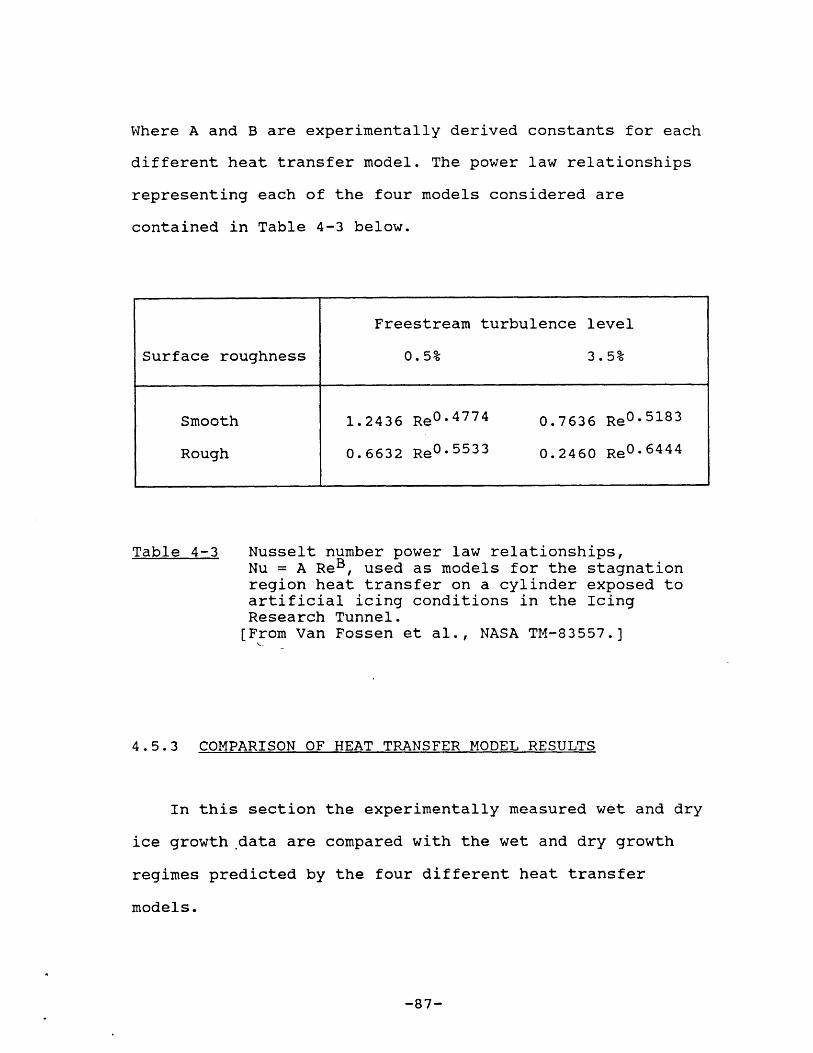
Where A and B are experimentally derived constants for each

different heat transfer model. The power law relationships

representing each of the four models considered are

contained in Table 4-3 below.

Table 4-3 Nusselt number power law relationships,Nu = A ReB, used as models for the stagnationregion heat transfer on a cylinder exposed toartificial icing conditions in the IcingResearch Tunnel.[From Van Fossen et al., NASA TM-83557.]

4.5.3 COMPARISON OF HEAT TRANSFER MODEL RESULTS

In this section the experimentally measured wet and dry

ice growth.data are compared with the wet and dry growth

regimes predicted by the four different heat transfer

models.

-87-

Freestream turbulence level

Surface roughness 0.5% 3.5%

Smooth 1.2436 Re0 .4 774 0.7636 Re0 .518 3

Rough 0.6632 Re0 .553 3 0.2460 Re0 .644 4

Figure 4-7 shows the ultrasonically measured ice growth

for the six "heavy" and "light" icing conditions tested in

the Icing Research Tunnel (Section 4.4). Impinging liquid

water content, BW, is plotted versus cloud temperature. The

impinging liquid water content on the cylinder stagnation

line was determined from the ultrasonically measured dry

growth accretion rates, Ddry, for the heavy and light icing

conditions,

BW = Ddry %ice/Vo (4.5)

In all cases the ice density, 3ice, was taken to be that

of the pure substance, i.e. 917 kg/m 3 . Note that since only

the cloud temperature was varied, the impinging- liquid water

content is a constant for the heavy and light icing

conditions. The impinging liquid water contents were

measured to be 0.47 g/m3 for the heavy icing conditions and

0.16 g/m3 for the light icing conditions. The freestream

velocity is 102.8 m/s (230 mph) for all six runs shown.

Also plotted in figure 4-7 are the wet/dry threshold

curves calculated from the steady-state energy balance for

the stagnation region (eq. 2.28). Four curves are shown,

corresponding to the four different heat transfer models

(0.5% and 3.5% freestream turbulence; smooth or rough

surface). All of these curves were calculated for a

-88-

Open symbols=WetSolid symbols = Dry

0 0

WET

growthgrowth 3-5%

Turb'[nce

7 0-50/

/Turb'tnce

-5 -10 -15 -20 -25 -30CLOUD TEMPERATURE, T( 0C)

Fig. 4-7 Plot of impinging liquid water content versuscloud temperature, showing ultrasonicallymeasured wet/dry ice growth and theoreticalwet/dry threshold curves.

-89-

Cylinder Dia. = 0-102mFreestream Vel. = 102-8m/s

Icing LWC MVDCondition (g/m3) ( P)Heavy, o 0-77 20Light, & 0-38 12

0-6

0-50

0-4

CL)zz

0-3

0-2

0-1

0.0

freestream velocity of 102.8 m/s and a cylinder diameter of

0.102 m.

Each of these threshold curves thus represents the

impinging liquid water content calculated to produce

transition from dry to wet ice growth, as a function of the

icing cloud temperature. The "critical" impinging liquid

water content, (BW)crit, at which this transition occurs,

depends on the convective heat transfer from the icing

surface. Hence the four different heat transfer models

predict different wet/dry thresholds. For each threshold

curve, the ice growth is predicted to be dry if the

impinging liquid water content is less than the critical

value, (BW)crit, calculated for that cloud temperature. If

the impinging liquid water content exceeds this critical

value then the ice growth is predicted to be wet.

Comparing'the four threshold curves (figure 4-7), it can

be seen that the heat transfer models that best predict the

experimentally observed pattern of wet and dry ice growth

are the 3.5% turbulence level models. Although all four

models correctly predict the three experimentally observed

wet growth cases, both of the 0.5% turbulence level models

incorrectly. predict wet growth for the heavy icing condition

at -28.6 0C, when dry growth was experimentally observed.

-90-

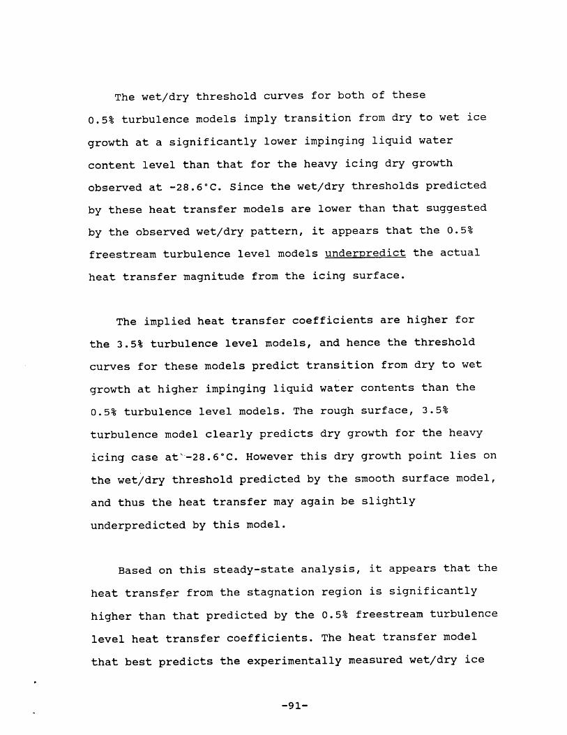
The wet/dry threshold curves for both of these

0.5% turbulence models imply transition from dry to wet ice

growth at a significantly lower impinging liquid water

content level than that for the heavy icing dry growth

observed at -28.6 0 C. Since the wet/dry thresholds predicted

by these heat transfer models are lower than that suggested

by the observed wet/dry pattern, it appears that the 0.5%

freestream turbulence level models underpredict the actual

heat transfer magnitude from the icing surface.

The implied heat transfer coefficients are higher for

the 3.5% turbulence level models, and hence the threshold

curves for these models predict transition from dry to wet

growth at higher impinging liquid water contents than the

0.5% turbulence level models. The rough surface, 3.5%

turbulence model clearly predicts dry growth for the heavy

icing case at'-28.6 0C. However this dry growth point lies on

the wet/dry threshold predicted by the smooth surface model,

and thus the heat transfer may again be slightly

underpredicted by this model.

Based on this steady-state analysis, it appears that the

heat transfer from the stagnation region is significantly

higher than that predicted by the 0.5% freestream turbulence

level heat transfer coefficients. The heat transfer model

that best predicts the experimentally measured wet/dry ice

-91-

growth behaviour is the 3.5% turbulence level, rough surface

model,

- Nu = 0.2460 Re0 .6 4 4 4 (4.6)

This heat transfer model (eq. 4.6) was used to compare

other wet/dry ice growth behaviour, measured for different

tunnel icing conditions. Figure 4-8 is similar to figure

4-7, with impinging liquid water content, BW, plotted versus

icing cloud temperature. Two separate plots are shown in the

figure, corresponding to two different tunnel freestream

velocities. The upper plot shows ultrasonic wet/dry ice

growth measurements for a freestream velocity of 71.5 m/s

(160 mph) and the lower plot for a velocity of 49.2 m/s

(110 mph). The impinging liquid water contents for the

experimental points shown were again inferred from the

ultrasonically measured dry growth accretion rates. For

those cases where no dry growth was observed, the impinging

liquid water content was 'obtained by direct calculation of

the local collection efficiency, B.

The wet/dry threshold curves calculated using the 3.5%

turbulence, rough surface heat transfer model are also shown

for the two different freestream velocities. For impinging

liquid water contents less than the calculated transition

value, (BW)crit, dry growth is predicted, and this area is

shaded in the figure for each plot.

-92-

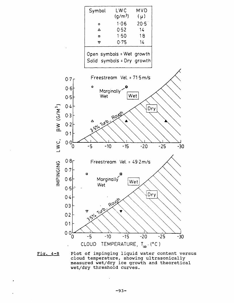
0-7- Freestream Vel. = 71-5m/s

06- Marginally-5 - Wet Wet -

-5 -10

LJ

-15 -20 -25

-5 -10 -15 -20 -25 -30CLOUD TEMPERATURE, T0 - (* C )

Fig. 4-8 Plot of impinging liquid water content versuscloud temperature, showing ultrasonicallymeasured wet/dry ice growth and theoreticalwet/dry threshold curves.

-93-

Symbol LWC MVD(g/m3) (p)

o 1-06 20-5A 052 14a 150 18

0-75 14

Open symbols =Wet growthSolid symbols =Dry growth

0-4

0-3

0-2

01

08

0-7

en

0

zFzz

-30

0-4

0-3-

0-2-

01-

000

All three experimentally observed dry growth points fall

within the dry growth regimes calculated using the 3.5%

turbulence, rough surface model. In addition, the two points

characterized as marginally wet (based on the ultrasonic

echo signals received during the ice growth), suggest that

the heat transfer over the ice surface may in fact be even

greater than that implied by this heat transfer model.

4.6 SUMMARY OF ICE GROWTH BEHAVIOUR AND HEAT TRANSFER

CHARACTERISTICS

Ultrasonic measurements of ice growth in the stagnation

region of a cylinder exposed to different icing conditions

in the IRT have provided the following information:

1. After any initial transient variations, the stagnation

region ice growth exhibits a "steady-state" period,

during which time the'accretion rate is essentially

constant.

2. For dry ice growth, the accretion rate is directly

proportional to the impinging liquid water content, and

is hence determined by the cloud liquid water content

and the local collection efficiency.

-94-

3. As the cloud temperature increases, wet ice growth is

observed in the stagnation region. The accretion rate

for wet growth is lower than the dry growth rate at

colder cloud temperatures.

4. By comparing the wet and dry growth accretion rates the

local freezing fraction may be inferred. The low

freezing fractions experimentally encountered at warm

cloud temperatures, suggest liquid runback from the

stagnation region during this initial growth period.

5. Ultrasonic measurements of wet and dry ice growth can be

compared with wet and dry ice growth regimes

theoretically predicted using the quasi steady-state

energy balance.

6. Using the steady-state energy balance, heat transfer

coefficients have been compared as models for the

convective heat transfer in the cylinder stagnation

region. Based on the predicted wet/dry thresholds, the

heat transfer occurring during initial ice growth

appears to be best modeled by Van Fossen's 3.5%

freestream turbulence, rough surface heat transfer

measurements for a bare cylinder. There are, however,

some experimental indications that the actual heat

transfer magnitude may be slightly in excess of that

predicted by this model.

-95-

Chapter 5

ICING OF A CYLINDER IN NATURAL ICING CONDITIONS

5.1 OVERVIEW

This chapter presents experimental measurements of ice

growth on a cylinder exposed to natural icing conditions in

flight. Ultrasonic measurements of ice thickness and ice

surface condition (wet or dry) are analyzed and compared to

similar measurements obtained for the icing wind tunnel

tests (Chapter 4).

Sections 5.2 and 5.3 outline the experimental apparatus

used and the cylinder installation on the flight test

aircraft. The'test procedure for each in-flight exposure of

the cylinder is also described in Section 5.3. Typical

natural icing cloud conditions and experimentally observed

ice growth behaviour are discussed in Section 5.4.

Ultrasonic measurements are presented showing both wet and

dry ice growth occurring as a result of in-flight variations

in the cloud liquid water content.

Section 5.5 compares the ultrasonically measured wet and

dry ice growth behaviour for each flight with that predicted

-96-

using the steady-state energy balance and the four heat

transfer models described in Chapter 4. The heat transfer

magnitude in the cylinder stagnation region is generally

inferred to be lower for the natural icing conditions

encountered in flight than for the icing conditions produced

in the Icing Research Tunnel. However, variations in the

implied heat transfer magnitude are observed, and may be due

to different turbulence levels associated with natural icing

clouds.

5.2 EXPERIMENTAL APPARATUS

The experimental apparatus employed to measure ice

growth in natural icing conditions was similar to- that

described in Chapter 4 for the icing wind tunnel tests (see

figure 4-1). The test cylinder for the flight tests had a

diameter of 11.4 cm (4.5 in.), and was instrumented with two

5 MHz ultrasonic transducers. The transducers were mounted

on the stagnation line, flush with the cylinder surface.

Both transducers had diameters of 0.6 cm, and were located

near the midsection of the 38.1 cm long cylinder.

A pulsex/receiver unit was used to drive the ultrasonic

transducers, and the resulting pulse-echo signals were

displayed on an oscilloscope. The oscilloscope screen was

again videotaped with a camera to provide a permanent record

-97-

of these time dependent signals. A digital clock mounted to

the oscilloscope screen was used to record the cylinder

exposure time. Figure 5-1 shows the video camera and

oscilloscope installed in the icing research aircraft.

Fig. 5-1 Photograph of the video camera and oscilloscope

installation on the floor of the NASA Lewis Icing

Research Aircraft.

-98-

5.3 NATURAL ICING FLIGHT TESTS

5.3.1 CYLINDER INSTALLATION ON THE ICING RESEARCH AIRCRAFT

The natural icing flight test: were conducted from the

NASA Lewis Icing Research Aircraft, a De Havilland DHC-6

Twin Otter. The test cylinder was mounted vertically on an.

experiment carrier platform that could be raised through the

roof of the aircraft, thus exposing the cylinder to the

natural icing cloud. Figure 5-2 illustrates this

configuration, with the cylinder extended into the

freestream above the aircraft. The cylinder was mounted on

an extension post, enabling the instrumented cylinder

midsection to be located 53.3 cm into the freestream when

deployed. The freestream disturbance, due to the aircraft

flowfield, was thus small at the cylinder midsection. Figure

5-3 is a photograph (looking aft along the roof of the

aircraft), showing the cylinder in its fully extended

position.

5.3.2 ICING RESEARCH AIRCRAFT INSTRUMENTATION

The icing research aircraft (figure 5-2) was equipped

with several icing cloud instruments, used to measure the

ambient natural icing conditions encountered in flight.

-99-

5 MHz, 0-25" Dia.

Flow

5" x 4-5"Dia.

3.5"

MIT Ultra!Ice Probe

Ice Detectors(PI.R.A.M.& Rosemount)

Laser CloudDroplet Probes

(MVD)

LWCHot Wire

Cylinder installation on the NASA Lewis Icing Research Aircraft.Fig.- 5-2

Fig. 5-3 Photograph showing the test cylinder extended

above the roof of the icing research aircraft.

In particular,-the cloud liquid water content measurements

presented for each flight -were obtained from a

Johnson-Williams hot-wire probe mounted near the nose of the

aircraft. A Particle Measuring Systems forward scattering

spectrometer probe (FSSP) was used to measure the cloud

droplet size distribution, from which the droplet median

volume diameter was later calculated. This probe (FSSP) was

mounted under the port wing of the aircraft. An onboard data

aquisition system sampled and recorded measurements from

these icing cloud instruments throughout each flight. Other

-101-

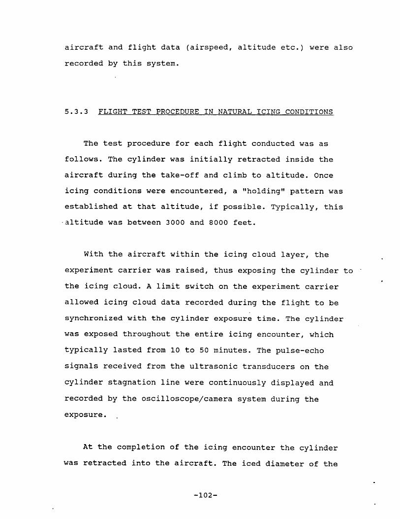
aircraft and flight data (airspeed, altitude etc.) were also

recorded by this system.

5.3.3 FLIGHT TEST PROCEDURE IN NATURAL ICING CONDITIONS

The test procedure for each flight conducted was as

follows. The cylinder was initially retracted inside the

aircraft during the take-off and climb to altitude. Once

icing conditions were encountered, a "holding" pattern was

established at that altitude, if possible. Typically, this

-altitude was between 3000 and 8000 feet.

With the aircraft within the icing cloud layer, the

experiment carrier was raised, thus exposing the cylinder to

the icing cloud. A limit switch on the experiment carrier

allowed icing cloud data recorded during the flight to be

synchronized With the cylinder exposure time. The cylinder

was exposed throughout the entire icing encounter, which

typically lasted from 10 to 50 minutes. The pulse-echo

signals received from the ultrasonic transducers on the

cylinder stagnation line were continuously displayed and

recorded by the oscilloscope/camera system during the

exposure. .

At the completion of the icing encounter the cylinder

was retracted into the aircraft. The iced diameter of the

-102-

cylinder was then measured at each transducer location,

using outside calipers; the total ice thickness accreted

during the exposure was inferred from this measurement.

Four research flights (85-22 to 85-25) were conducted

with the cylinder and ultrasonic system during the period

March 30-April 2, 1985.

5.3.4 SUMMARY OF TIME-AVERAGED NATURAL ICING CONDITIONS AND

CYLINDER ICE ACCRETIONS

Figure 5-4 contains a summary of the time-averaged icing

conditions during each of the four in-flight exposures of

the test cylinder. The shape of the accreted ice at the

completion of the exposure (from photographs of the iced

cylinder), is also sketched for each flight.

The ice thicknesses measured on the cylinder stagnation

line at the end of the exposure are indicated for the both

the ultrasonic system and the outside caliper measurement.

As in the icing wind tunnel tests, the ultrasonic pulse-echo

thickness measurements are within ±0.5 mm of the caliper

readings, confirming the speed of sound is relatively

constant for ice formed under typical flight icing

conditions.

-103-

TIME - AVERAGED ICING CONDITIONS

FLIGHT EXPOSURE TEMP LWC M V D VEL ALTITUDENUMBER TIME (*C) (GM/M3) (p) (MPH) (FEET)

(MIN: SEC)

85-22 20:41 - 5-4 0-36 11.9 157 272885-23 47:08 - 3-3 0-18 11-4 147 340485-24 10 : 07 -14-6 0-46 14 est. 161 648085-25 36:40 -15-1 0.19 14.1 167 7019

FLIGHT ULTRASONICALLY MECHANICALLYNUMBER MEASURED ICE MEASURED ICE ICE SHAPE

THICKNESS (MM) THICKNESS (MM)

3-1

3.3

8-9

VIDEO TAPEDAMAGED

2.7

ICE SLID OFF

8-7

9- 6

TRANSDUCER

FLOW

A ___________________ ________________________

Ficr. 5-4 Summary of time-averaged icing conditions andcylinder ice accretions for flight tests.

-104-

85-22

85-23

85-24

85-25

However, while constant icing conditions were maintained

for each exposure in the Icing Research Tunnel, the natural

icing conditions encountered in flight varied throughout

each exposure. These unsteady icing conditions, and the

different ice growth behaviour observed as the ambient

conditions changed, are discussed in the next section.

5.4 ICE GROWTH BEHAVIOUR OBSERVED DURING NATURAL ICING

CONDITIONS

From the ice thicknesses indicated in figure 5-4 and the

correspording exposure times, it can be seen that the

average ice accretion rates observed during the natural

icing flight tests were much lower than those obtained in

the Icing Research Tunnel tests. For example, only during

the exposure on flight 85-24 did the average accretion rate

on the cylinder -stagnation line exceed 0.3 mm/min. These

lower overall accretion rates (ice thickness/exposure time)

are primarily due to the lower average liquid water contents

encountered in these flight tests.

Figure 5-5 shows the ice thickness measured with the

ultrasonic.system plotted against exposure time for flight

85-24. Also shown are the time-averaged icing conditions

during the 10 minute exposure. The cloud temperature for

this exposure was relatively cold (-14.60 C), and rime

-105-

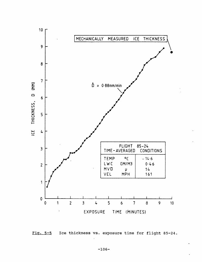
10 -

MECHANICALLY MEASURED ICE THICKNESS

9

8

7

6

LI5IA

I~ 5

Lii 4

I I I I I I I I I I I

0 1 2 3 4 5 6 7 8 9 10

EXPOSURE TIME (MINUTES)

5-5 Ice thickness vs. exposure time for flight 85-24.

-106-

O = 0-88mm/min

FLIGHT 85-24TIME-AVERAGED CONDITIONS

TEMP *C -14.6LWC GM/M3 0-46MVD p 14VEL MPH 161

3

2

1

0

Fig.

ice formation was observed for most of the exposure. The

average accretion rate was determined to be 0.88 mm/min,

from the slope of the ice thickness curve.

The ice thickness measured during flight 85-24

(figure 5-5) increases fairly linearly with exposure time.

This linear or "steady-state" ice growth behaviour was also

observed during the tests conducted in the Icing Research

Tunnel. However while the ambient icing conditions were

constant for the icing wind tunnel tests, the icing

conditions varied throughout each in-flight exposure. The

linear increase in ice thickness with exposure time observed

for the in-flight exposure is therefore of particular

interest, and suggests that.under certain icing conditions

the time fluctuations in cloud properties may not

significantly influence the accretion behaviour. The

variations in icing cloud properties, observed in flight,

are discussed'below.

Figure 5-6 is a plot of the flight data recorded during

the cylinder exposure on flight 85-22. The ambient icing

conditions (cloud temperature, liquid water content and

median volume diameter), measured by the aircraft's icing

cloud instrumentation, are plotted versus the cylinder

exposure time. Also shown are the aircraft airspeed and

altitude for the exposure period.

-107-

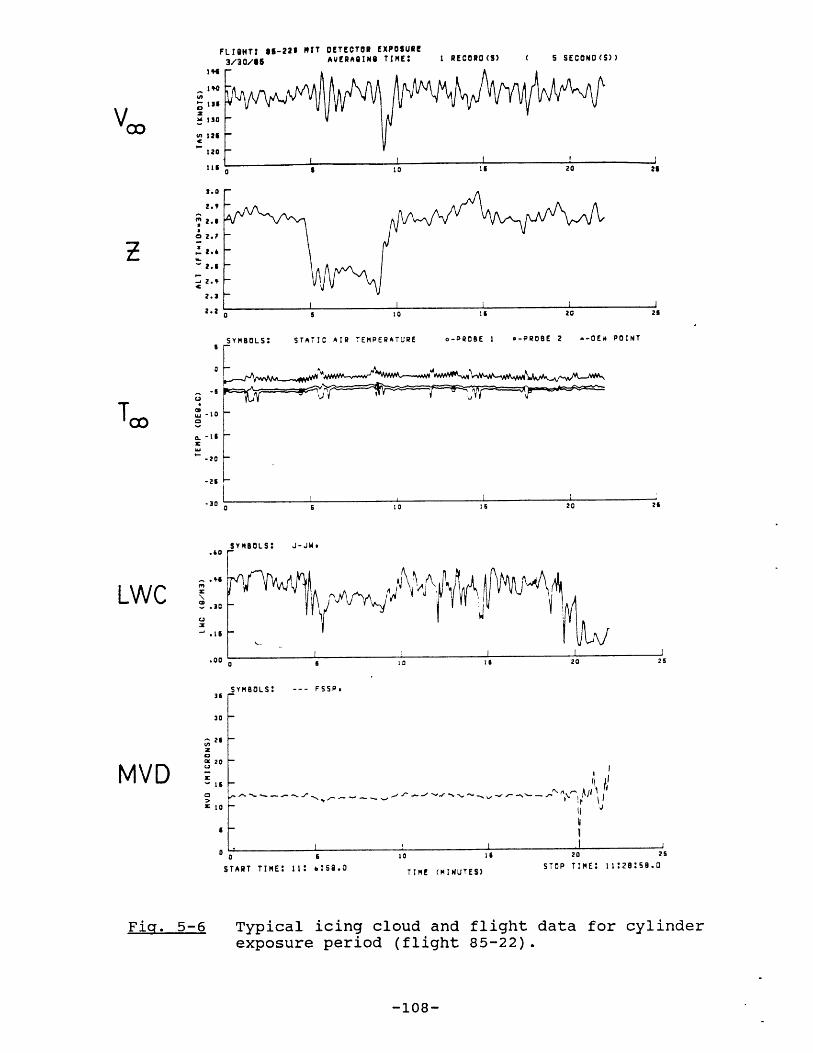
LWC

-~.15

.00

31

30

LIGHT: 86-221 MIT3/30/85

DETECTOR EXPOSUREAvERAGING TIME: 1 RECORD(S) ( 5 SECOND(S))

F

139

S130

126

120

115

3.0

2.9

2.8

o 2.7

2.1

2.3

2.2

SYMBOLS: STATIC AIR TEMPERATURE o-PROBE 1 a-PROBE 2 -- DEW POINT

-s

-21 M

-30 0 6 101 6 20 21

SYMBOLS: J-JN..40 r-

0 1 10 16 20 2

SYMBOLS: --- FSSP.

Ij f I

20-

0 1

START TIME: I ::56.0TIME (MINU

TES)

20 26

STOP TIME: 11:28:59.0

Fig. 5-6 Typical icing cloud and flight data for cylinderexposure period (flight 85-22).

-108-

VCO

0g 10 11 20 21

UJ-

0.-a

10

1

-20 F

MVDS20

K

-15

0

K10

From the figure, it can be seen that the airspeed and

altitude were held fairly constant during the exposure, as

desired. The static air temperature is also seen to be

relatively constant throughout the exposure. Typically,

these'three parameters - airspeed, altitude and cloud

temperature - were not observed to vary significantly during

the four cylinder exposures conducted.

However, the cloud liquid water content did vary

considerably throughout each exposure. For example, the

liquid water content (measured by the Johnson-Williams

hot-wire probe), varied from less than 0.15 g/m3 to over

0.5 g/m3 during the cylinder exposure on flight 85-22 (see

figure 5-6). The fluctuations in cloud liquid water content

shown in figure 5-6, are characteristic of all the exposures

conducted in natural icing conditions.

Although the cloud droplet median volume diameter

measured (FSSP) during the cylinder exposure for flight

85-22 was relatively constant (MVD = 12 microns), this was

not the case for all the exposures. For example, the droplet

median volume diameter measured for flight 85-25 varied from

11 to 21 microns during the course of the 37 minute cylinder

exposure.

These variations in both the cloud liquid water content,

and the droplet size distribution, produce corresponding

-109-

fluctuations in the liquid water content impinging on a body

in natural icing conditions. As a result, periods of wet and

dry ice growth may occur as the impinging liquid water

content, BW, varies.

Figure 5-7 is a plot of the measured cloud liquid water

content versus cylinder exposure time, for flight 85-24.

Also shown are experimentally observed periods of wet, dry

and transitional ice growth on the cylinder stagnation line.

The ultrasonic echo signals during natural icing conditions

displayed the same characteristics as those observed in the

icing wind tunnel tests, and were again used to determine

the type of ice growth. The ice growth was categorized as

transitional when the time variation in the detailed shape

of the ultrasonic echo signal was between that

characteristically observed for wet or completely dry ice

growth.

From the figure, it can be seen that dry ice growth was

observed for cloud liquid water contents below 0.4 g/m3

while wet growth occurred for sustained liquid water

contents above approximately 0.55 g/m3 . At the lower liquid

water content levels (<0.4 g/m3), the heat transfer from the

stagnation region is sufficient to freeze all the locally

impinging mass flux due to the cloud droplets.

-110-

2 4

EXPOSURE

6 8

TIME, t (MINUTES)

Fig. 5-7 Plot of liquid water content versus exposure timefor flight 85-24 showing fluctuations in naturalicing cloud liquid water content and wet, dry andtransitional ice growth periods measured usingultrasonic system.

However when the liquid water content exceeds a critical

value, the rate of heat removal from the ice surface is

insufficient to freeze all the impinging mass flux, and

liquid forms on the ice surface. The "critical" impinging

liquid water content at which this wet growth begins depends

on the local heat transfer coefficient for the icing

-111-

Dry = Dry ice growthWet = Wet ice growthTr. = Transitional ice growth

0-8-S0-6 -

0-4 -

0-2-0-

0

surface, as discussed in Chapters 2 & 4. The ultrasonically

measured wet and dry ice growth periods may thus be used in

conjunction with the icing cloud data to compare different

heat transfer coefficient models applicable to natural icing

conditions. This comparison of heat transfer models for the

cylinder stagnation region is discussed in the next section.

5.5 COMPARISON OF HEAT TRANSFER COEFFICIENT MODELS FOR THE

STAGNATION REGION OF A CYLINDER IN NATURAL ICING

CONDITIONS

The analysis presented in this section follows closely

that outlined in Chapter 4 for the icing wind tunnel tests.

The four heat transfer models compared are again the high

and low (3.5% & 0.5%) freestream turbulence, rough or smooth

surface, cylinder stagnation region heat transfer

coefficients measured by Van Fossen et a11 2.

However, while constant ambient icing conditions were

maintained during each exposure in the icing wind tunnel

tests, the natural icing cloud conditions in the flight

tests varied throughout each exposure. Therefore, in order

to use the.quasi steady-state energy balance to compare

predicted wet/dry thresholds with the experimentally

observed wet and dry ice growth, a simple steady-state "time

constant" was estimated. This time constant approach was

-112-

taken to minimize the effects of transient thermal behaviour

not accounted for in the steady-state energy balance.

A time constant of 10 seconds was selected, based on

both the transient thermal response of a thin ice layer, and

the frequency response of the Johnson-Williams hot-wire

probe (-5 seconds 17 ). Thus only cloud liquid water contents

sustained for more than 10 seconds were used in the

comparison with the wet/dry threshold curves calculated

using the steady-state energy balance.

Figure 5-8 is a plot of impinging liquid water content

versus cloud temperature. The experimentally observed,

"steady-state" wet, dry and transitional ice growth regimes

for the four cylinder exposures on flights 85-22 to 85-25,

are plotted. The impinging liquid water content, 3W, was

determined from the cloud liquid water content measured by

the Johnson-Williams hot-wire probe, and by direct

calculation of the local collection efficiency". The local

collection efficiency on the cylinder stagnation line was

calculated 15 for a monodisperse droplet distribution with a

droplet diameter equal to the median volume diameter

measured by the FSSP laser probe. The error in the

collection.efficiency calculated with this single droplet

size assumption is considered small relative to the

uncertainties present in the measurements of cloud liquid

water content and droplet size distribution6' 18 .

-113-

Dia. = 0-114mAv. FreestreamAv. Altitude =

Symbol Fli

Vel. = 714 m/s1613mght No.85-22

V 85-23o 85-24a 85-25

Open symbols =Wet growthsymbols = D

Transitional

Wet-

-77

7

-5 -10 -15 -20

ry growth -Roughgrowth 3-5% T

Smoot

V/

/-.

urb.h

Rough0-5% Turb.Smooth

-25

TEMPERATURE,

Fig. 5-8 Plot of impinging liquid water content versuscloud temperature showing wet, dry andtransitional ice growth observed during flighttests, and theoretical wet/dry threshold curves

114-

0-6

.0Solid

= -

0-5F

0-4F

0-3 F

z3ZF.

~

0-2

0-1

0-0-

CLOUD Ta, (*C )

Cylinder

Also shown in figure 5-8 are the four wet/dry threshold

curves calculated for the different heat transfer

coefficient models described earlier. These curves were

calculated for the test cylinder diameter, 11.4 cm, and for

the average airspeed and altitude for the four exposures,

71.4 m/s and 1613 m, respectively (160 mph and 5290 ft).

The wet ice growth observed during flights 85-22 and

85-23 occurred at relatively warm cloud temperatures, and

all four heat transfer models predict wet growth for these

conditions.

On flight 85-24, the experimentally observed range of

wet and dry ice growth is correctly predicted by the 3.5%

turbulence level heat transfer coefficients. The wet/dry

thresholds calculated for both the rough and smooth surface,

3.5% models, lie within the experimentally determined

"transitional* ice growth band between dry and wet growth.

The low (0.5%) turbulence'heat transfer coefficient models

appear to underestimate the heat transfer magnitude for this

flight, since dry growth was experimentally observed at

impinging liquid water contents above the wet/dry threshold

predicted by these heat transfer models.

In contrast to flight 85-24, the high freestream

turbulence (3.5%) models appear to overpredict the heat

transfer magnitude for flight 85-25, and the low (0.5%)

-115-

turbulence models correctly predict the observed wet and dry

ice growth ranges. From figure 5-8 it can be seen that both

the rough and smooth surface heat transfer coefficients at

the 3.5% turbulence level imply dry growth (based on the

steady-state energy balance analysis), when wet growth was

experimentally observed.

For this exposure (85-25), the low turbulence heat

transfer coefficient models appear appropriate, since the

wet/dry thresholds calculated for both of these coefficients

correctly predict the observed wet growth regime. In fact,

since dry growth was only observed at very low impinging

liquid water contents (<0.05 g/m3 ), the actual heat transfer

from the icing surface may have been even lower than that

suggested. by the 0.5% turbulence level models.

This result is significant, since it implies the heat

transfer magnitude in flight may, in some cases, be lower

than that for an equivalent icing surface in the Icing

Research Tunnel. As discussed earlier, the magnitude of the

heat transfer coefficient in the stagnation region is of

critical importance, since it determines the threshold

between dry and wet ice growth. Any difference therefore,

between the.heat transfer magnitude in the Icing Research

Tunnel and in flight, could result in different ice growth

behaviour for seemingly identical "ambient" icing

conditions. These differences in ice growth behaviour would

-116-

be most pronounced during wet growth, with different local

freezing fractions and possibly different degrees of liquid

runback. The implication is that, under certain icing

conditions, the ice accretions formed in flight and in the

Icing Research Tunnel would be different. Since the purpose

of the icing wind tunnel is to provide a natural icing

simulation capability, this situation would clearly be

undesirable, unless a correction can be applied to allow for

different heat transfer magnitudes.

The experimental results shown in figure 5-8 also

indicate that there may be some variation in the convective

heat transfer magnitude encountered during flight through

different icing clouds. For example, during flights 85-24

and 85-25, the cloud temperatures, liquid water contents and

droplet sizes encountered were roughly comparable, and yet

different ranges of wet and dry ice growth were

experimentally observed. This can be seen in figure 5-8 as

the observed wet and dry growth ranges for these two flights

overlap at the same impinging liquid water content level

(0.2 g/m3). The implication is that the heat transfer from

the icing surface differed between these two flights, both

at nominally similar icing conditions, but conducted on

different days, through different natural icing clouds. One

plausible explanation for this apparent variation in the

convective heat transfer are differences in the turbulence

levels associated with different cloud formations, e.g.

-117-

convective versus stratiform clouds.

5.6 SUMMARY OF ICE GROWTH BEHAVIOUR AND HEAT TRANSFER

ANALYSIS FOR NATURAL ICING CONDITIONS

During flight through natural icing clouds the icing

conditions are not constant. The most significant variation

is seen in the cloud liquid water content, although the

cloud temperature and droplet size distribution may also

vary. Fluctuations in the cloud liquid water content can

result in periods of both wet and dry ice growth occurring

during a single icing cloud encounter.

Although ice growth was only measured for four expbsures

in natural icing conditions, on at least one of these

exposures (85-24) the ice thickness was observed to increase

approximately'linearly with exposure time. This constant

accretion rate behaviour,'despite fluctuations in the cloud

liquid water content, suggests that for relatively cold

cloud temperatures the time-averaged value of the cloud

liquid water content may be appropriate to characterize the

natural icing encounter. However at warmer cloud

temperatures, fluctuations in the cloud liquid water content

may be important in determining periods of wet ice growth.

-118-

Based on the wet/dry ice growth behaviour observed

during the four flight tests conducted, it appears that the

heat transfer magnitude appropriate for an icing surface in

flight may be lower than that inferred for the Icing

Research Tunnel.

The heat transfer during the initial icing period has

been found to vary between that suggested by the 3.5%

freestream turbulence level and 0.5% turbulence level heat

transfer coefficients of Van Fossen et al.. A similar

analysis showed the heat transfer for the Icing Research

Tunnel tests was best modeled by the 3.5% turbulence level

coefficients. The difference in heat transfer magnitude may

thus be due to a higher freestream turbulence level in the

Icing Research Tunnel. Considering the upstream spray bar

system used in the Icing Research Tunnel, a higher

freestream turbulence level in the tunnel test section than

at the cylinder location above the aircraft, might be

expected.

In addition to the generally lower heat transfer

magnitude inferred from the flight test results, variations

in the heat transfer magnitude were also observed for

flights conducted on different days. These variations may

again be associated with the freestream turbulence level,

since different cloud formations have characteristically

different turbulence levels associated with them.

-119-

All of these results highlight the variability of

natural icing cloud conditions and the inherent difficulty

in accurately simulating these conditions in an icing wind

tunnel. However, the differences observed in the implied

heat transfer magnitude for the Icing Research Tunnel and

natural icing conditions dictate that care should be taken

in extrapolating results from icing wind tunnel tests to

"similar" natural icing conditions.

-120-

Chapter 6

SUMMARY AND CONCLUSIONS

Chapter 1 provided background information on aircraft

icing. Icing conditions were defined and typical icing cloud

parameters given. The effects of ice accretion on aircraft

performance were briefly outlined and illustrated. The

rationale for developing analytic models to predict ice

accretion was explained, and the steps involved in the

modeling procedure described. It was shown that the ice

shapes predicted by these analytic models can be extremely

sensitive to the assumed heat transfer distribution over the

body under certain ambient icing conditions. The lack of

experimental heat transfer data for real ice surfaces has

hindered the successful development of these models, as have

fundamental questions about the behaviour of liquid water on

the ice surface.

In Chapter.2 a quasi steady-state energy balance for the

accreting surface was described. The energy balance

considers six modes of energy transport to and from the

icing surface, and is largely based on the earlier work of

Messinger1 l. The assumptions implicit in both the quasi

steady-state approach and the energy balance itself were

-121-

discussed. The mass and energy balance equations were

derived for both 'dry and wet ice growth conditions, the

latter for-the stagnation region only. An expression

defining the threshold between wet and dry ice growth was

obtained in terms of a critical impinging liquid water

content and the local heat transfer coefficient for the ice

surface.

The ultrasonic pulse-echo techniques employed to measure

ice growth in artificial and natural icing conditions were

described in Chapter 3. The time of flight principle used in

ultrasonic pulse-echo thickness measurement was explained,

and it was shown that a continuous thickness measurement can

be achieved by repeatedly emitting pulses at a high pulse

repitition rate. The ultrasonic echo signals received from

accreting ice surfaces were then described. The presence of

liquid water on the ice surface during wet ice growth was

shown to produce a unique time variation in the received

echo signal, thus allowing the ultrasonic echo

characteristics to be used to distinguish between wet and

dry ice growth.

Chapter 4 described experimental measurements of ice

growth in the stagnation region of a 10.2 cm diameter

cylinder exposed to icing conditions produced in an icing

wind tunnel. The ambient icing conditions for these tests in

the Icing Research Tunnel were constant for each test run

-122-

conducted. Plots of ice thickness versus exposure time were

presented for two different icing cloud sets, characterized

as "heavy" and "light" icing conditions. In all cases these

plots showed a "steady-state" period in which the ice

thickness increased relatively linearly with exposure time.

For the exposures during which the ice growth was

observed to be dry, this constant accretion rate behaviour

was inferred to indicate that the local collection

efficiency, and hence the flowfield, were unchanged by the

ice accretion during this initial icing period. The

exposures for which the ice surface was determined to be wet

also exhibited a similar period of constant growth rate. In

these cases (wet growth), the constant accretion rate was

most likely an indication that both the local collection

efficiency and the local heat transfer from the icing

surface were essentially unchanged as the ice accreted

during this initial icing period.

The effect of cloud temperature on the ice growth

behaviour was also investigated. At warm cloud temperatures

the ice surface was observed to be wet and the measured

accretion rates were low. However, as the cloud temperature

was progres.sively reduced, the accretion rate increased to a

maximum value and then remained constant despite further

decreases in the cloud temperature. At the "warm" cloud

temperatures, the heat transfer from the ice surface was

-123-

insufficient to freeze all the impinging droplet mass flux,

and hence the freezing fraction was less than unity, and the

accretion rate low. As the temperature "potential" is

increased between the wet ice surface at 0*C and the icing

cloud, the heat transfer from the surface increases, thus

increasing the accretion rate. Finally, when the heat

transfer is sufficient to freeze all the impinging droplets

on impact, the ice growth is dry and the accretion rate a

maximum.

By comparing the low accretion rates, measured at the

warm cloud temperatures, with the higher dry growth

accretion rates, the freezing fractions for the wet growth

cases were inferred. These implied freezing fractions, and

the ultrasonic echo characteristics observed for these wet

growth cases, indicated that liquid runback from the

stagnation region did occur during the initial icing period

for these wet'growth cases.

Also contained in Chapter 4 was a comparison of the

experimentally measured wet and dry ice growth conditions

with the regimes of wet and dry ice growth predicted by the

steady-state energy balance presented in Chapter 2.

Specifically, four different heat transfer coefficient

models were compared in the energy balance equation. The

four models used were from experimental heat transfer

measurements by Van Fossen et al. for the stagnation region

-124-

of a cylinder.

The results of this comparison showed that the heat

transfer in the stagnation region of the test cylinder

during icing conditions in the Icing Research Tunnel was

best modeled by a heat transfer coefficient measured with a

high (3.5%) freestream turbulence level. Heat transfer

coefficients with a lower associated freestream turbulence.

level (0.5%) incorrectly predicted wet growth and therefore

underestimated the actual heat transfer from the icing

surface.

Chapter 5 presented measurements of ice growth in the

stagnation region of an 11.4 cm diameter cylinder exposed in

flight to natural icing conditions. Unlike the constant

icing conditions maintained during each exposure in the

icing wind tunnel tests, the icing conditions in flight were

observed to vary throughout each exposure. The cloud liquid

water content in particular characteristically fluctuated

significantly. These fluctuations in liquid water content

resulted in periods of dry, wet and transitional ice growth

within the same exposure.

Despite.these fluctuations in cloud liquid water

content, a roughly linear increase in ice thickness with

exposure time was observed for one exposure at a relatively

cold cloud temperature. Although more experimental data is

-125-

needed, this result seems to indicate that, in some cases,

the time-averaged liquid water content may adequately

represent a natural icing encounter. However at warmer cloud

temperatures, fluctuations in the liquid water content may

be of greater importance.

A similar heat transfer analysis was conducted on the

experimentally measured wet and dry ice growth data obtained

in the flight tests as was performed for the Icing Research

Tunnel data. The same (Van Fossen et al.) heat transfer

coefficients were used in the steady-state energy balance

equation to predict wet and dry ice growth regimes. The

results of this comparison showed that the heat transfer

magnitude for the icing surface in flight may be lower than

that inferred for the Icing Research Tunnel. The heat

transfer coefficient that best modeled the flight data

appeared to lie between that associated with a high (3.5%)

freestream turbulence and that for the lower, 0.5%,

turbulence level investigated.

In addition, the results of the heat transfer analysis

indicated that the magnitude of the heat transfer occurring

in natural icing conditions may vary from day to day,

despite similar icing conditions. This variation may be due

to different turbulence levels associated with different

icing cloud formations.

-126-

The results of the natural icing tests highlight the

variations inherent in all natural icing encounters. Ice

growth may-vary from wet to dry within a single natural

icing cloud as the impinging liquid water content

fluctuates. The use of an average liquid water content to

represent a particular natural icing condition may thus be

inaccurate for some icing conditions, particularly for warm

cloud temperatures. In addition, the potentially different

heat transfer characteristics for icing wind tunnel studies

and natural icing conditions dictates that care be taken in

extrapolating results from icing wind tunnels to "similar"

natural icing conditions.

-127-

REFERENCES

1. Olsen, W.A., Jr., Shaw, R., and Newton, J., "Ice Shapesand the Resulting Drag Increase for an NACA 0012Airfoil." NASA TM 83556, 1984.

2. Gibbings, D.C., "Development for Helicopter Flight inIcing Conditions." AGARD CP-299, 1981.

3. MacArthur, C.D., "Numerical Simulation of Airfoil IceAccretion." AIAA-83-0112, January 1983.

4. Lozowski, E.P., Stallabrass, J.R., and Hearty, P.F.,"The Icing of an Unheated Non-Rotating Cylinder inLiquid Water Droplet-Ice Crystal Clouds." NationalResearch Council of Canada (NRC) Report LTR-LT-86,February 1979.

5. Bragg, M.B., Gregorek, G.M., and Shaw, R.J.,"An Analytical Approach to Airfoil Icing." AIAA-81-0403,January 1981.

6. Chang, H.P., Kimble, K.R., Frost, W., and Shaw, P.J.,"Influence of Multidroplet Size Distribution on IcingCollection Efficiency." AIAA-83-0110, January 1983.

7. Gelder, T.F., Smyers, W.H.,Jr., and Von Glahn, U.,"Experimental Droplet Impingement on SeveralTwo-Dimensional'Airfoils with Thickness Ratios of 6 to16 Percent." NACA TN 3839, December 1956.

8. Hansman, R.J., "The Effect of the Atmospheric DropletSize Distribution on Airfoil Ice Accretion."AIAA-84-0108, January 1984.

9. Ruff, G.A., "Development of an Analytical Ice AccretionPrediction Method (LEWICE)." Sverdrup Technology, Inc.,LeRC Group Progress Report, February 1986.

10. Kirchner, R.D., "Aircraft Icing Roughness Features andIts Effect on the Icing Process." AIAA-83-0111, January1983.

11. Messinger, B.L., "Equilibrium Temperature of an UnheatedIcing Surface as a Function of Airspeed." Journal of theAeronautical Sciences, January 1953, pp 24-42.

12. Van Fossen, G.J., Simoneau, R.J., Olsen, W.A., and Shaw,R.J., "Heat Transfer Distributions Around Nominal IceAccretion Shapes Formed on a Cylinder in the NASA LewisIcing Research Tunnel." AIAA-84-0017, January 1984.

-128-

13. Personal communication with P.J. Perkins, SverdrupTechnology, Inc., Middleburg Heights, OH, January 1986.

14. Macklin, W.C., "The Density and Structure of Ice Formedby Accretion." Quarterly Journal of the RoyalMeteorological Society, Vol. 88, No. 375, January 1962.

15. Brun, R.J., Lewis, W., Perkins, P.J., and Serafini,J.S., "Impingement of Cloud Droplets on a Cylinder andProcedure for Measuring Liquid-Water Content and DropletSizes in Supercooled Clouds by Rotating MulticylinderMethod." NACA TR-1215, 1955.

16. Personal communication with W.A. Olsen, NASA LewisResearch Center, Cleveland, OH, March 1986.

17. Neel, C.B., Jr., and Steinmetz, C.P., "The Calculatedand Measured Performance Characteristics of aHeated-Wire Liquid-Water-Content Meter for MeasuringIcing Severity." NACA TN-2615, 1952.

18. Ide, R.F., and Richter, G.P., "Comparison of Icing CloudInstruments for 1982-1983 Icing Season Flight Program."AIAA-84-0020, January 1984.

-129-

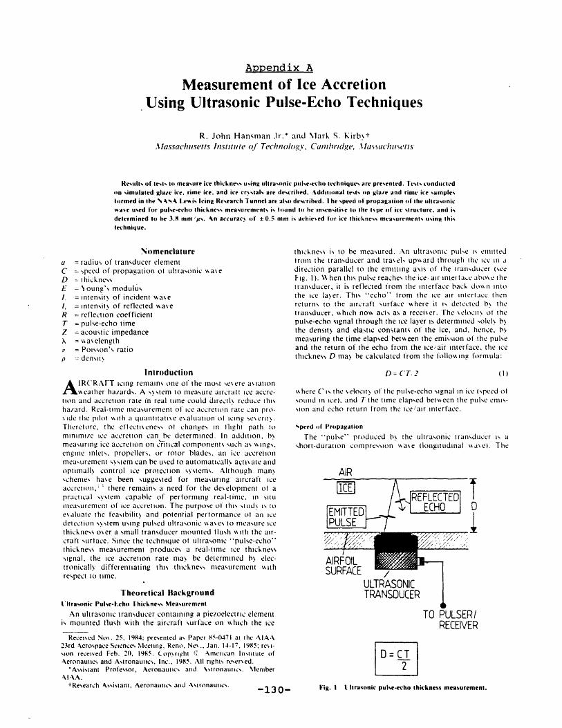
Appendix A

Measurement of Ice AccretionUsing Ultrasonic Pulse-Echo Techniques

R. John Hansman .r.* and \Mark S. Kirbs+Massachusetts Institute of Technology, Camndgride, .\Mas sachusetts

Results of tests to measure ice thickness using ultrasonic pulse-echo techniques are presented. Tests conductedon simulated glare ice, rime ice, and ice crysials are described. Addtiaonal tests on glaie and rime ice samplesformed in the A'%4 l.es is Icing Research Tunnel are also described. 1 he speed of propagation of the ultrasonicwase used for pulse-echo thickness measurements is bound to he insensitise to the ispe of ice structure, and isdetermined to he 3.8 mm /ps. An accurac% of +0.5 mm is achiesed for ice thickness measurements using thistechnique.

Nomenclaturea = radius of transducer elementC = speed of propagation ot ultrasonic wa-eD = thicknessE = N oung's modulusS= intensity of incident w aseI, =intensity of reflected waveR = reflection coefficientT = pulse-echo timeZ =acoustic impedanceX = was elengthe = Poisson's ratiop density

Introduction

A IRCRAFT icing remains one of the most seere asiationw\eather ha/ards. A sstem to measure aircraft ice accre-

tion and accretion rate in real ume could directl\ reduce thisha/ard. Real-time measurement of ice accretion rate can pro-side the pilot wkith a quantitatise esaluation of icing seserity.Therefore, the eflectiseness ol changes in flight path tominimi/e ice accretion can be determined. In addition, b\measurine ice accretion on critical components such as w1ings.engine inlets, propellers, or rotor blades, an ice accretionmeasurement s stem can be used to automatically agti ate andoptimallk control ice protection systems. Although mansschemes hase been suggested for measuring aircraft iceaccretion,;' there remains a need for the deselopinent of apractical system capable of performing real-time, in situmeasurement of ice accretion. The purpose of this study is toesaluate the feasibility and potential pertormance of an icedetection system using pulsed ultrasonic wases to measure icethickness oser a small transducer mounted flush with the air-craft surface. Since the technique ot ultrasonic "pulse-echo"thickness measurement produces a real-time ice thicknesssignal, the ice accretion rate may be determined b\ clec-tronically differentiating this thickness measurement withrespect to time.

Theoretical BackgroundUltrasonic Pulse-l-cho Ihickness Measurement

An ultrasonic transducer containing a piezoelectric elementis mounted flush with the aircraft surface on which the ice

Receised Nos. 25, 1984; presented as Paper 85-0471 at the AIA.\23rd Aerospace Sciences Meeting, Reno. Nes.. Jan. 14-17, 1985; rest-sion received Feb. 20, 1985. Copyright (i American Institute ofAeronautics and Astronautics, Inc., 1985. All rights resersed.

*Assistant Professor, Aeronautics and \stronauncs. \1emberA AA.

tResearch Assistant, Aeronautics and AWsronauics. -130-

thickness is to be measured. An ultrasonic pulse is emittedfrom the transducer and trasels upwsard through the ice in adirection parallel to the emitting asts of the transducer (seeFig. 1). \ hen this pulse reaches the ice, air interlae abose thetransducer, it is reflected from the interface back dosn intothe ice laser. This "echo" from the ice air interface thenreturns to the aircraft surface where it is detected b\ thetransducer, wshich nows acts as a receiser. The selocity of thepulse-echo signal through the ice layer is determined solely b\the density and elastic constants of the ice, and, hence, b,.measuring the time elapsed between the emission of the pulseand the return of the echo from the ice/air interface, the icethickness D may be calculated from the following formula:

D=CT,2

where C is the selocity of the pulse-echo signal in ice (speed ofsound in ice), and T the time elapsed between the pulse emis-sion and echo return from the ice/air interface.

Speed of Propagation

The ''pulse" produced b\ the ultrasonic transducer is ashort-duration compression swase (longitudinal wsase). The

AIR

7D

ULTRASONICTRANSDUCER

TO PULSER/RECEIVER

D = C T

2

Fig. I t Itrasonic pulse-echo thickness measurement.

REFLECTEDEMITTED ECHOPUL SE

AIRFOUILSURFACE

selocity C at which such a compression wsae propagatesthrough a solid medium is theoreticall predicted4 to be

E(/-v)p(/+ v)(1 -2p)

where E is the Young's modulus for the medium. v thePoisson's ratio, and p the density of the medium. Hence, thepulse-echo signal propagates through a solid medium at a con-stant % elocity that depends only on the density and elasic con-stants of the medium.

Reflection of Ultrasonic Signal from Ice/ Air Interface

The ultrasonic pulse is reflected back toward the transducer(as the echo signal) at the ice.iair interface (Fig. 1) because ofthe difference in the acoustic impedances of ice and air. Theacoustic impedance, Z, of a medium is defined as the productof the medium's density, p, and the speed of sound in themedium, C, given by Eq. (2): hence,

Z=pc (3)

The reflection coefficient, R, for an interface is defined4 as theratio of the intensity of the reflected wave, I,, to that of the in-cident wave, /,, and is gisen by

R =+= I 2 2(4)it, Z,+-t Z,)

where Z, and Z, are the acoustic impedances of the two mediaforming the interface. From this equation it can be seen thatthe intensity of the'reflected wave, or echo signal, depends onthe acoustic impedance mismatch between the two media.Since both the density and speed of sound in air are con-siderably lower than those for solids, the acoustic impedancemismatch for a solid/air interface is large, resulting in strongreflection at a solid/air interface. For an ice. air interface thereflection coefficient is calculated to be greater than 0.99, i.e.,more than 997o of the incident wave energy is reflected at anice/air interface.

CouplingFor the %ibration of the transducer element to be transmit-

ted into a solid medium, a "coupling" mechanism betw een thetransducer and the solid must be available. Although it isoften necessary to use a fluid to provide this couplingmechanism, no such fluid is required for ice thicknessmeasurement since the ice is atomically bonded to thetransducer face and, therefore, is constrained to vibrate with,the transducer element.

Ultrasonic Field ShapeAt the high frequencies (5-20 MHz) used for pulse-echo ice

thickness measurement, the wavelength X in the ice is typicallysmall (<1 mm) compared to the radius a of the radiatingtransducer element. Under these conditions the ultrasonicwave propagates from the transducer as a collimated beam ofthe same diameter as the transducer element. This beam, ornear-field region, extends for a distance given by the ratioa2/A, after which the wave diserges in the far-field region.Typical near-field ranges are approximately 2 in. for a0.5-in.-diam, 5-MHz transducer and I in. for a 0.25-in.-diam,10-MHz transducer.

AttenuationAttenuation of the received echo signal can be divided into

three components: absorption and scattering within the ice,and reflection at the ice/air interface. Absorption occurs aspart of the vibrational energy of the wave is stored as heat bythe ice molecules and then lost through irreversible heat

transfer n ithin the ice layer. Scattering is caused b% any inclu-sions wsithin the ice (such as air bubbles), since. bN definition,these inclusions have a different acoustic impedance to that ofthe ice and, therefore, present spurious reflectise interfaces tothe incident ultrasonic wase. The third factor allecting thereceived strength of the echo signal is the shape of the ice, airinterface itself. While almost 10Fo of the incident waseenergy is reflected at the ice air interface. the shape of the in-terface determines the direction(s) of reflected wvase propaga-tion. Rough ice surfaces will reflect the incident wvase diffusely.while ice surfaces that are not parallel to the transducer facewill cause the echo signal to propagate at an angle to the emit-ting axis of the transducer. In both cases the intensity of theecho received by the transducer will be diminished over thatreceived from an identical ice thickness with a flat, parallelice/air surface.

Experimental ApparatusThree components comprised the pulse-echo thickness

measurement system tested: a transducer, a pulser/receiserunit, and an oscilloscope (Fig. 2). The function and importantperformance characteristics of each of the components areoutlined below. The experimental apparatus constructed tosimulate and test the application of this pulse-echo s stem toice accretion measurement is then described.

TransducerThe transducer used to produce and receive the ultrasonic

pulse-echo signal was a broadband, highly damped contacttransducer. This type of transducer allows maximum signalpenetration in attenuating and scattering materials such asrime and glaze ice. Excellent thickness resolution is also possi-ble with this type of transducer. A single transducer was usedfor all of the tests described. The transducer tested had acenter frequency of 5 MHz and an element diameter of 0.5 in.

Pulser /Receiser

The pulser/receiver provides the ele,'rical signals necessar%for the operation of the transducer in a pulse-echo mode. Thepulser section of the pulser'receiver supplies the transducerelement with a short, high-%oltage pulse of controlled energ.

AIRICE 7A

EXTERNAL TRIGGERFig. 2 Ultrasonic pulse-echo system.

-131-

This soltage pulse causes the transducer element to ibrate.thus producing the ultrasonic pulse utibied in pulse-echothickness measurement. The soltage applied to the transducerelement is is pically on the order of 200 V. The %oltage pulse isreapplied ito he transducer element seseral hundred times persecond to produce a "continuous" pulse-echo thicknessreading. The receiser. section amplfies and conditions thesmall echo soltage produced b tihe transducer element itself.The tipical gain required is approximatel\ 40 dB. In addition.the pulser receis er pros ides a s nchronizing soltage used totrigger an oscilloscope sweep momentarily betore the mainsoltage pulse is applied to the transducer element. For ex-perimental purposes, an oscilloscope w\as used to observe thepulse-echo signal characteristics in different ice formationsand measure the pulse-echo time. Figure 3 shows a typicalpulse-echo trace obtained from a 5.0-mm-thick ice layer.

Eaperimenial ApparatusTo allow ice to be frozen oser the transducer face and the

pulse-echo system tested, the apparatus showsn in Fig. 4 wkasused. A circular 9-in.-diam aluminum plate sersed as a testsurface on which the ice accretion was to be measured. Thetransducer was mounted in the center of this plate wsith thetransducer face flush wsith the plate surface. An 8-in.-diamplexiglas cylinder could be used to contain wkater poured ontothe plate surface when it was desired to freeze liquid waterover the face of the transducer (in order to simulate glaze ice).A remos able plexiglas lid could be fitted oser this cylinder; thepurpose of the lid was to provide a reference lesel from whichthe ice thickness over the plate surface could be accuratelymeasured by inserting a steel probe graduated in millimetersthrough one of a grid of small holes drilled into the lid. Thealuminum plate was also instrumented wkith two

+04-+03 _ T= 2 35pS

0 PULSE . ,ICE/AIR ECHO+0 2 ~ MTE+01 EMITTED 2nd ECHO RETURN

1 00-01 EP 3rd RETURN

U -02 - TRIGGERED1-03- \AMPLIFIER MIT GLAZE ICE

L- RECOVERY D=5mm-04 -

0 1 2 3 4 5 6 7 8 9 10 11 12PULSE-ECHO TIME, T (p S)

-ig. 3 1 pical pulse-echo trace for ice.

Ice Thickness

Clamp

Aluminum Pti

chromelalumel thermocouples to monitor the plate icetemperature.

Testingin order to calibrate the configured pulse-echo ssstem,

aluminum and plexiglas samples of different thicknesses wseremeasured using the ultrasonic pulse-echo technique. B com-paring the measured speed of sound in the material,

C=2D/T (5)

w ith w ell-established values, the error in the obtainable pulse-echo thickness measurements was determined to be less than5ir 0 for equisalent ice thicknesses from I to 30 mm. Testing ofthe pulse-echo system comprised two consecutive series of'trials. The first series consisted of tests performed on iceformed at MIT. Both glaze and rime ice structures weresimulated and ice thicknesses from 1.5 to 31 mm wkere tested.Additional tests were also performed on ice crystal forma-tions. The second series of tests utilized ice samples obtainedfrom the Icing Research Tunnel (IRT) at NASA LewisResearch Center. Glaze and rime ice formations from 4.5- to15-mm thick were tested in this series of tests.

MIT Glaze Ice Simulation Tests

Glaze ice was simulated by pouring water into the plexiglascylinder/plate apparatus (Fig. 4) to a depth approximatelyequal to the desired ice thickness, and then the apparatus wasplaced in a cold box thermostatically maintained at - 20*C.Once the water was completely frozen, the pulse-echo time Twas recorded from the oscilloscope display. The apparatuswas then removed from the cold box so the ice thickness couldbe measured with the graduated probe as described earlier.The ice thickness was always recorded within I min of remos alfrom the cold box and no appreciable rise in ice temperature(as indicated b\ the plate thermocouples) took place betwseenthe recording of the pulse-echo time and the corresponding icethickness measurement.

M11 Rime Ice simulation Tests

To simulate rime ice, the aluminum plate containing theultrasonic transducer was first placed in the cold box. Oncethe plate had reached its steady-state temperature (typically- 18'C), water droplets at O'C were sprayed onto theplater transducer lace using a misting nozzle connected to asmall electric pump and ice/water reservoir (Fig. 5). Thedroplets were sprayed intermittently rather than continuousyto prevent the ice temperature from significantly increasing asa result of the heat of fusion released by the treezing waterdroplets. Droplets were typically obsersed to freeze within 2 sof impact with the plate surface. Measurement of the pulse-echo time and ice thickness was made in a manner similar tothat described for the glaze ice-simulation tests.

Water-200C Clamp f (rom pump)

Fig. 4 lEperimental apparatus. Fig. 5 Rime ice simulation method.

-132-

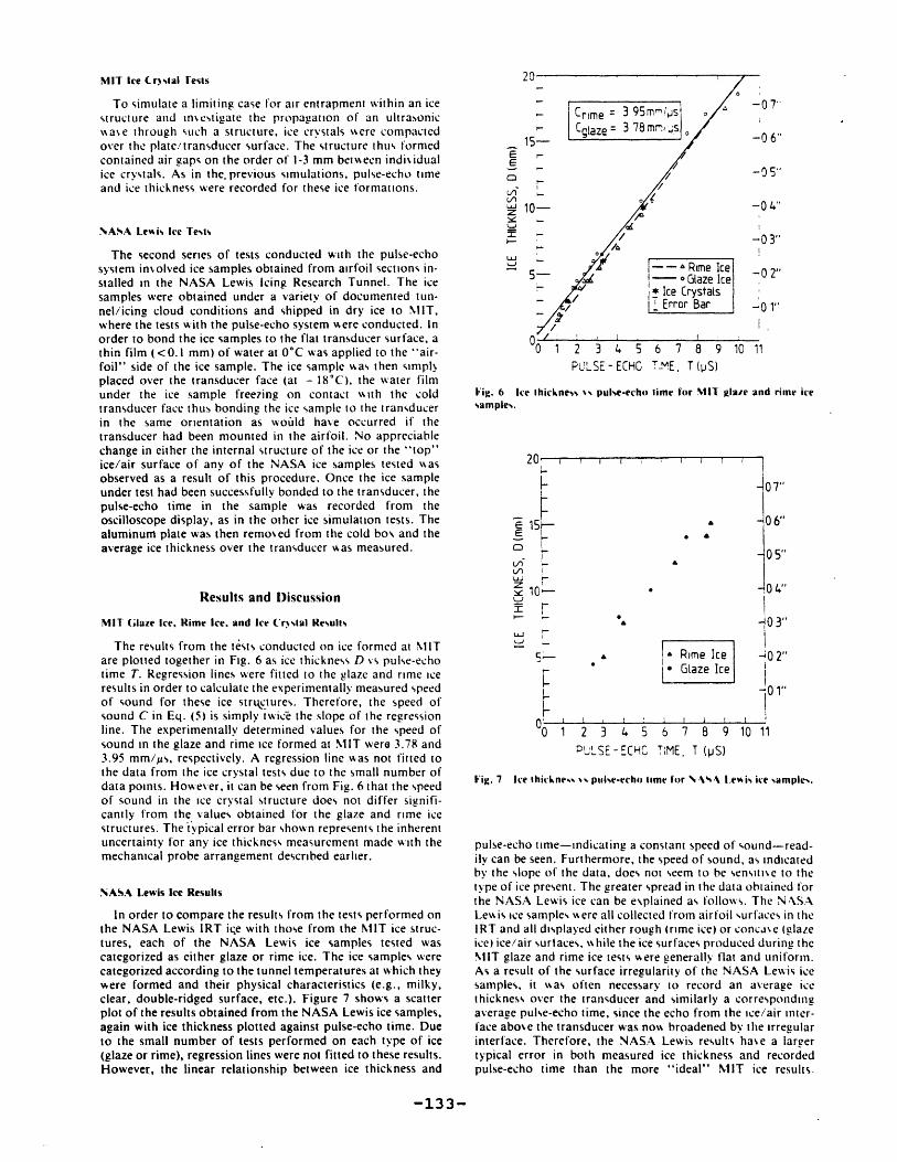
MIT Ice Crstial Fests

To simulate a limiting case for air entrapment within an icestructure and insestigate the propagation of an ultrasonicwsase through such a structure, ice crystals were compactedover the plate/transducer surface. The structure thus formedcontained air gaps on the order of 1-3 mm between indisidualice crstals. As in the. previous simulations, pulse-echo timeand ice thickness were recorded for these ice formations.

NASA Lewis Ice Tests

The second series of tests conducted with the pulse-echosystem insolved ice samples obtained from airfoil sections in-stalled in the NASA Lewis Icing Research Tunnel. The icesamples were obtained under a variety of documented tun-nel/icing cloud conditions and shipped in dry ice to MIT,where the tests with the pulse-echo system were conducted. Inorder to bond the ice samples to the flat transducer surface, athin film (<0.1 mm) of water at 0*C was applied to the "air-foil" side of the ice sample. The ice sample was then simplyplaced over the transducer face (at - 18*C), the water filmunder the ice sample free7ing on contact with the coldtransducer face thus bonding the ice sample to the transducerin the same orientation as woild have occurred if thetransducer had been mounted in the airfoil. No appreciablechange in either the internal structure of the ice or the "top"ice/air surface of any of the NASA ice samples tested wasobserved as a result of this procedure. Once the ice sampleunder test had been successfully bonded to the transducer, thepulse-echo time in the sample was recorded from theoscilloscope display, as in the other ice simulation tests. Thealuminum plate was then remosed from the cold box and theaverage ice thickness over the transducer was measured.

Results and Discussion

MIT Glaze Ice, Rime Ice, and Ice C(rsial Results

The results from the tests conducted on ice formed at MITare plotted together in Fig. 6 as ice thickness D vs pulse-echotime T. Regression lines were fitted to the glaze and rime iceresults in order to calculate the experimentally measured speedof sound for these ice strqctures. Therefore, the speed ofsound C in Eq. (5) is simply twice the slope of the regressionline. The experimentally determined values for the speed ofsound in the glaze and rime ice formed at MIT were 3.78 and3.95 mm/ps, respectively. A regression line was not fitted tothe data from the ice crystal tests due to the small number ofdata points. However, it can be seen from Fig. 6 that the speedof sound in the ice crystal structure does not differ signifi-cantly from the values obtained for the glaze and rime icestructures. The typical error bar shown represents the inherentuncertainty for any ice thickness measurement made with themechanical probe arrangement described earlier.

NASA Lewis Ice Results

In order to compare the results from the tests performed onthe NASA Lewis IRT ice with those from the MIT ice struc-tures, each of the NASA Lewis ice samples tested wascategorized as either glaze or rime ice. The ice samples werecategorized according to the tunnel temperatures at which theywere formed and their physical characteristics (e.g., milky,clear, double-ridged surface, etc.). Figure 7 shows a scatterplot of the results obtained from the NASA Lewis ice samples,again with ice thickness plotted against pulse-echo time. Dueto the small number of tests performed on each type of ice(glaze or rime), regression lines were not fitted to these results.However, the linear relationship between ice thickness and

15-

10-

LUJ

5 .'

- /

012" 1 2 3PUL SE

Fig. 6 Ice thickness nsamples.

20,

i 15F-z10 --

LU

50-

0

Crime = 3 95mr'sJs a

Cglaze = 3 78 mry s

-- a~ Rime Ice- oGlaze Ice

* Ice CrystalsT Error Bar

4 5- ECHO

6 7 8 9 10TME. T (pS)

-0 7"

-0 6"

-051,

-0 4"

-03"

--0 2"

-0 1"

11

pulse-echo time for MIT glaie and rime ice

I I

2 3 4 5PI LSE-E7CHC

a 0 6"

-10 4"

0 3"& Rime Ice 10 2"eGlaze Ice

1"

6 7 8 9 10 11

TME, T (pS)

Fig. 7 Ice thicknes %w pulse-echo lime for NS, % Lewis ice samples.

pulse-echo time-indicating a constant speed of sound-read-ily can be seen. Furthermore, the speed of sound, as indicatedby the slope of the data, does not seem to be sensitise to thetype of ice present. The greater spread in the data obtained forthe NASA Lewis ice can be explained as follows. The N ASALew is ice samples w ere all collected from airfoil surfaces in theIRT and all displayed either rough (rime ice) or conca'e (glazeice) ice/air surt aces, w hile the ice surfaces produced during theMIT glaze and rime ice tests were generally flat and uniform.As a result of the surface irregularity of the NASA Lewis icesamples, it was often necessary to record an average icethickness over the transducer and similarly a correspondingaverage pulse-echo time, since the echo from the ice/air inter-face abose the transducer was now% broadened by the irregularinterface. Therefore, the NASA Lewis results hase a largertypical error in both measured ice thickness and recordedpulse-echo time than the more "ideal" MIT ice results.

-133-

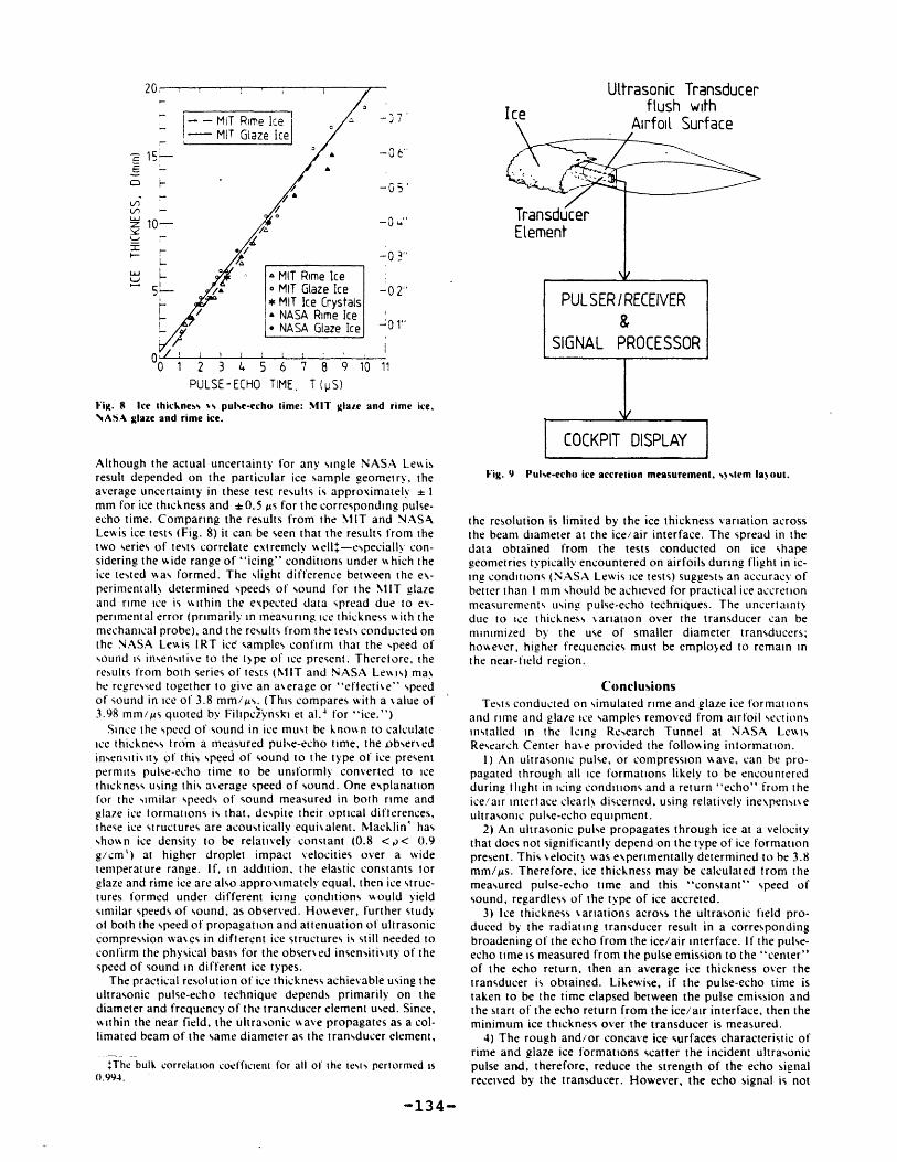
20

-- MIT Rime Ice A- MIT Glaze Ice

L" 0

15- * -0."

-03"a MIT Rime Ice

5 / MIT Glaze Ice -0 2"* MIT Ice Crystalsa NASA Rime Iceo NASA Glaze Ice 01

0'~0 1 2 3 4 5 6 7 8 9 10 11

PULSE-ECHO TIME, T (pS)

Fig. 8 Ice thickness s% pulse-echo time: MIT glaze and rime ice.NASA glaze and rime ice.

Although the actual uncertainty for any single NASA Lewsisresult depended on the particular ice sample geometry, theaverage uncertainty in these test results is approximately * Imm for ice thickness and *0.5 ps for the corresponding pulse-echo time. Comparing the results from the MIT and NASALewis ice tests (Fig. 8) it can be seen that the results from thetwo series of tests correlate extremely well*-especially con-sidering the wkide range of "icing" conditions under which theice tested was formed. The slight difference between the ex-perimentally determined speeds of sound for the MIT glazeand rime ice is wsithin the expected data spread due to ex-perimental error (primarily in measuring ice thickness with themechanical probe), and the results from the tests conducted onthe NASA Lewis IRT ice samples confirm that the speed ofsound is insensitise to the type of ice present. Therefore, theresults from both series of tests (NIT and NASA Lewsis) ma\be regressed together to give an aserage or "eftectise" speedof sound in ice of 3.8 mm/ps. (This compares with a salue of3.98 mm/ps quoted by Filipc>ynski et al. 4 for "ice.")

Since the speed of sound in ice must be knowsn to calculateice thickness trom a measured pulse-echo time, the obsertedinsensitisity of this speed of sound to the type of ice presentpermits pulse-echo time to be uniformly converted to icethickness using this aserage speed of sound. One explanationfor the similar speeds of sound measured in both rime andglaze ice formations is that, despite their optical differences,these ice structures are acoustically equisalent. Nacklin' hasshowkn ice density to be relatively constant (0.8 <p< 0.9g/cm') at higher droplet impact velocities over a widetemperature range. If, in addition, the elastic constants forglaze and rime ice are also approximately equal, then ice struc-tures formed under different icing conditions would yieldsimilar speeds of sound, as observed. However, further studyof both the speed of propagation and attenuation of ultrasoniccompression wases in different ice structures is still needed toconfirm the physical basis for the obsersed insensitisity of thespeed of sound in different ice types.

The practical resolution of ice thickness achievable using theultrasonic pulse-echo technique depends primarily on thediameter and frequency of the transducer element used. Since,within the near field, the ultrasonic wave propagates as a col-limated beam of the same diameter as the transducer element,

:The bulk correlation coefficient for all or the tests periormed is0.994.

Ultrasonic Transducerflush with

Airfoil Surface

TransducerElement"

PUL SER /RECEIVER&

SIGNAL PROCESSOR

COCKPIT DISPLAYFig. 9 Pulse-echo ice accretion measurement. system layout.

the resolution is limited by the ice thickness variation acrossthe beam diameter at the ice/air interface. The spread in thedata obtained from the tests conducted on ice shapegeometries typically encountered on airfoils during flight in ic-ing conditions (NASA Lewis ice tests) suggests an accuracy ofbetter than I mm should be achieved for practical ice accretionmeasurements using pulse-echo techniques. The uncertaintydue to ice thickness sariation over the transducer can beminimized by the use of smaller diameter transducers;however, higher frequencies must be employed to remain inthe near-field region.

ConclusionsTests conducted on simulated rime and glaze ice formations

and rime and glaze ice samples removed from airfoil sectionsinstalled in the Icine Research Tunnel at NASA LewsisResearch Center hase provided the following information.

1) An ultrasonic pulse, or compression wave. can be pro-pagated through all ice formations likely to be encounteredduring light in icing conditions and a return "echo" from theice/air interface clearly discerned, using relatively inexpensiseultrasonic pulse-echo equipment.

2) An ultrasonic pulse propagates through ice at a velocitythat does not significantly depend on the type of ice formationpresent. This selocit% was experimentally determined to be 3.8mm/ps. Therefore, ice thickness may be calculated from themeasured pulse-echo time and this "constant" speed ofsound, regardless of the type of ice accreted.

3) Ice thickness %ariations across the ultrasonic field pro-duced by the radiating transducer result in a correspondingbroadening of the echo from the ice/air interface. If the pulse-echo time is measured from the pulse emission to the "center"of the echo return, then an average ice thickness over thetransducer is obtained. Likewise, if the pulse-echo time istaken to be the time elapsed between the pulse emission andthe start of the echo return from the ice/air interface, then theminimum ice thickness over the transducer is measured.

4) The rough and/or concave ice surfaces characteristic ofrime and glaze ice formations scatter the incident ultrasonicpulse and, therefore, reduce the strength of the echo signalreceived by the transducer. However, the echo signal is not

-134-

obscured and the pulse-echo time can be measured in all of theice shapes typically encountered during flight in icingconditions.

Therefore, ultrasonic pulse-echo thickness measurement isconsidered to ofler a practical solution to the problem of real-time ice accretion measurement for aircraft encountering icingconditions. The operational accuracy achiesable with such asystem depends primarily on the transducer specifications (fre-quency and element diameter) and the location of thetransducer. An accuracy of *0.5 mm for ice thicknessmeasurement is predicted. The configured ultrasonic pulse-echo system would comprise three components: an ultrasonictransducer, a pulser/receiver and signal processing unit, and acockpit display (Fig. 9). The transducer is nonintrusise andmounted flush with the surface on which ice accretion is to bemeasured. The transducer units are small and lightw eight and,therefore, may be mounted on almost any % ulnerable surface,including helicopter rotor blades and engine inlets. The signalprocessor calculates the ice thickness trom the measured pulse-echo time and also differentiates this real-time measurementwkith respect to time to obtain the ice accretion rate. Thecockpit display unit prosides the pilot with an automatic"icing encountered" alert and indicates icing severity as well

as controlling and or monitoring the operation of fited iceprotection s> stems.

AcknowledgmentThis swork w\as supported b\ the National A iation and

Space Administration under Girants NA(,-1-100 andNG L-22-009-640.

ReferencesPerkins, P. J., \lc~uIlouth, S , and I.ewsR D.. t \ \impit ied

Instrument for Recording and Indicating -requenes and intensii\ it

Icing Conditions Lncouniered in I tight," N-AC(A R\1 s1L16, 19512\1agenheirn, B. and Rocks, J K., "Deselopient and Test ot a

\lierowkase Ice Accreion \leasurenieni Instrument I1AMI"N',A-A CR-3598. 1982.

'Ide. R. 1. and Riebiter. G. P . "Esaluatnon ol' Icine ( loud In-strumeniation for 1982-83 Icing Season Htight Progiam,'" \\Paper 84-0020, Ian. 19S4

I tihpc/ nski, L . Pawl toswski. 7.. and \\e hr, J , Lt rasont<\1t'hods f Testing \laterials. Buiterworths, London, I160

\lackin. \\ . C , "Densiiy and Structure ot Ice I oirmed b\ AXere-

i 'on," Quarterlv Journal ol the Rotal %Ieteorolovual Saiei t , \ol.8,. No 375, lan. 1962, pp 30-50.

-135-

Appendix B

CALCULATION OF LIQUID WATER CONTENT FOR CYLINDER LOCATION

OUTSIDE CALIBRATED CLOUD REGION

In order to estimate the actual liquid water content at

the cylinder location, as a percentage of the (known)

calibrated cloud value, the following approach was taken.

The expected dry growth accretion rates on the cylinder

stagnation line were analytically calculated (from Ref. 15)

using the calibrated cloud liquid water content and median

volume diameter values. These "calibrated cloud" accretion

rates, Dcal, were then compared to the experimentally

measured dry growth rates on the cylinder, Dcyl, and the

ratio of these two rates was used to 4ive the liquid water

content at the cylinder location as a percentage of the

calibrated cloud value.

For the ultrasonically measured dry ice growth rate,

Ocyl, on the cylinder stagnation line,

Dcyl = (W) cylVa/3 ice (B.1)

Where (8W).Qyl is the actual impinging liquid water content

on the cylinder stagnation line.

a

-136-

The analytically calculated accretion rate, Dcall

based on the calibrated cloud values, is given by,

Dcal = (BW)calv /3ice (B.2)

Where (BW)cal is the liquid water content that would impinge

on the cylinder stagnation line if the cylinder were located

in the calibrated cloud region of the test section.

Equations B.1 and B.2 may be combined to give,

Dcyl/Dcal = (BW)cyl/(BW)cal (B.3)

Note that it has been assumed that the both the freestream

velocity and ice density are the same for the cylinder

location and calibrated cloud region.

If the droplet size distribution at the cylinder

location is close to that in that calibrated region then the

local collection efficiency terms may be cancelled and

equation B.3 yields the desired ratio of liquid water

contents,

Dcyl/Dcal = Wcyl/Wcal (B.4)

Thus by comparing the measured accretion rates with the

rates calculated for the calibrated cloud region, a

-137-

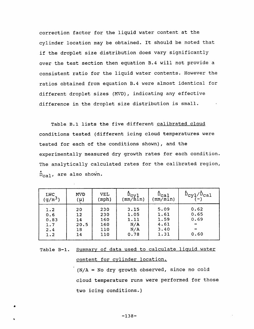
correction factor for the liquid water content at the

cylinder location may be obtained. It should be noted that

if the droplet size distribution does vary significantly

over the test section then equation B.4 will not provide a

consistent ratio for the liquid water contents. However the

ratios obtained from equation B.4 were almost identical for

different droplet sizes (MVD), indicating any effective

difference in the droplet size distribution is small.

Table B.1 lists the five different calibrated cloud

conditions tested (different icing cloud temperatures were

tested for each of the conditions shown), and the

experimentally measured dry growth rates for each condition.

The analytically calculated rates for the calibrated region,

Dcal, are also shown.

LWC MVD VEL Ocyl $cal bcyl/bcal(g/m3 ) (P) (mph) (mm/min) (mm/min) (-)

1.2 20 230 3.15 5.09 0.620.6 12 230 1.05 1.61 0.650.83 14 160 1.11 1.59 0.691.7 20.5 160 N/A 4.61 -2.4 18 110 N/A 3.40 -1.2 14 110 0.78 1.31 0.60

Table B-1. Summary of data used to calculate liquid water

content for cylinder location.

(N/A = No dry growth observed, since no cold

cloud temperature runs were performed for those

two icing conditions.)

-138-

From equation B.4 and the values listed in Table B-1 for

the accretion rate ratios, Ocyl/Dcal, the average ratio

inferred for the liquid water content at the cylinder

location is thus,

Wcyl/Wcal = Dcyl/Dcal = (0.62 + 0.65 + 0.69 + 0.60)/4

Wcyl = 0.64 Wcal

Hence the liquid water content at the cylinder location,

Wcyl, is estimated to be approximately 64% of the calibrated

cloud value, Wcal-

-139-