kisssoft book 2015
DESCRIPTION
KISSsoft Book 2015TRANSCRIPT
Article Collection of KISSsoft 2015
KISSsoft Calculation Tool for the Design, Optimization and Analysis of Machine Elements
KISSsoft AG 2 / 108
Article Collection of KISSsoft 2015
Layout of the gear micro geometry – A most challenging task
Enhanced gear efficiency calculation including contact analysis results and drive cycle consideration
Combining different manufacturing errors for calculation of KHβ along ISO6336-1, Annex E
A complete parameter study approach to designing differential bevel gears
Effect of housing stiffness in gear design
Gear strength when operating a gearbox at resonance and considering transient events using a mill
drive as example
Optimising a transmission for use with higher hp engine
Wear on gears: Prediction of the worn tooth form and the consequences on NVH and lifetime
Accelerated testing method for polymer gears
VDI 2736 – New Guideline, Old Challenges
A new process for sharing industrial gearbox calculation tool between Technical and Sales
Departments in Bonfiglioli Riduttori S.p.A.
Your Contact
KISSsoft AG Rosengartenstrasse 4 8608 Bubikon Switzerland Tel. +41 55 254 20 50 [email protected] www.KISSsoft.AG
Your Contact for the Asian Market
EES KISSsoft GmbH Hauptstrasse 7 6313 Menzingen Switzerland Tel. +41 41 755 33 20 [email protected] www.EES-KISSsoft.ch
KISSsoft AG 3 / 108
Layout of the gear micro geometry – A most challenging task
Dr.-Ing. Ulrich Kissling, KISSsoft AG, Bubikon, Switzerland
Article published in „Gear Solutions“, September 2015
Abstract
The last phase in sizing a gear pair is to specify the flank line and profile modifications (the "micro geometry"). To do so, it is first necessary to select the primary objective for which optimization has to be achieved: noise, service life, scuffing, micropitting or efficiency. One thing is certain: it is not possible to achieve all types of optimization simultaneously, and some actions will worsen some features while improving others. It is easy for the design engineer to lose sight of the bigger picture, and fail to find the optimum solution, because the calculation method for proving the effects achieved by micro geometry, the contact analysis under load ("Loaded Tooth Contact Analysis", or LTCA), is complex and time-consuming, and interpreting the results is complex. Today, we need much more time to optimize the micro geometry than the macro geometry, when designing a toothing. This makes it all the more surprising that the technical literature barely mentions the topic of micro geometry. In Niemann [1], for example, the topic of profile shift is discussed over 5 pages, while only 3 pages are devoted to flank line and profile modifications! When performing a targeted sizing of the micro geometry, a step-by-step approach should be used, first specifying the flank line modification and then the profile modification. This paper describes how a 3-step process can be implemented to perform a targeted sizing. Usually, there is only one layout criterion for specifying the optimum flank line modification: to achieve a load across the face width as evenly distributed as possible, and, in particular, to avoid edge contact (highest load on the end of the face). The progression of the gap in the meshing is caused by the elastic deformation of the shafts, generated by the operating forces and manufacturing allowances (tolerances). It is best to size the flank line modification in two steps. In step 1, we specify the ideal flank line modification using the average position in the tolerance field, without taking into account deviations due to manufacturing (tolerances). The aim is to reach an even load distribution across the face width. This will allow for the maximum possible service life to be achieved. As the deformation of the shafts differs according to the load, it is necessary to specify the torque for which the modification has to be sized. In the case of a complex load spectra this is not a trivial matter. For this reason, a special method has been developed, which can be used to achieve the maximum service life while also taking into account the load spectrum. Using the "one-dimensional contact analysis" [2] (according to ISO 6336-1, Appendix E [3]) is ideal for this purpose. Once the flank line modification for the medium tolerance position is determined in step 1, the manufacturing tolerances are compensated with an additional modification in step 2. Tolerances (manufacturing allowances) cause a random increase/reduction of the gap across the face width. Usually, an additional, symmetrical modification (flank line crowning or end relief) is the only practical solution for preventing edge contact in all possible combinations of allowances. How large the relief (Cb value) for a modification of this kind should be depends on statistical estimates and experience. When the flank line modification is defined, the third step is to specify the profile modifications. Now the primary aim (sizing criterion such as noise, service life, etc.) is very important. LTCA has to be used as calculation method, and this may require a lot of time if several variants are to be checked. A program module has been developed specially for this purpose. It generates a list of variants, processes them, and then displays a clear summary of the results.
KISSsoft AG 4 / 108
The LTCA calculation runs completely automatically, as it may run for hours in extreme cases, if hundreds of profile modification combinations are calculated. A typical application is minimizing the transmission error by systematically varying the value and length of the pinion and gear tip relief, independently of one another. As a profile modification has also a certain influence on the face load distribution, also the previously specified flank line modification may be varied along with the profile modification. The results will then be displayed both as a graph and in a configurable table. For interesting individual variants, a report is generated, which contains all the detailed results from the LTCA. The micro geometry optimization process described here can be applied to cylindrical gear or bevel gear pairs. If required, it can also be combined with an analysis of the housing deformation from an FEM calculation. In the case of planetary stages, the optimization is performed for all the meshings in the system, including the deformation of the planet carrier from an integrated FEM calculation.
1. Introduction: Use of Modifications
This paper explains how to find straight forward the optimum profile and flank line modifications for a given gear pair using a 3-step-procedure. The layout of the modifications is the last step in the gear design process. It is therefore extremely important to keep in mind, that a bad choice of macro geometry (as module, helix angle, profile shift, …) can never be compensated with a nice micro geometry. The choice of the best macro geometry [4] is primordial before starting the layout of modifications. Flank line and profile modifications have been in use in the gear industry for a long time. Nevertheless, designing modifications is not easy. In literature, astonishingly few information about the topic can be found. In the Niemann book [1] just few generic hints are given – compared to the detailed discussion of much simpler problems as for example profile shift layout! A problem is that the verification of the effect of modifications can only be made with a loaded tooth contact analysis (LTCA) [5]. LTCA is a complex semi-FEM calculation procedure, which needs a lot of calculation time. Furthermore such software was not available or too complicated to use for most gearbox designers. Therefore, modifications were designed based on simple rules without checking, if the rule used was appropriate for a specific case. In the last years more and easier to use LTCA software were developed. For a LTCA calculation, all gear data together with the geometry and load condition of the shafts is needed. Therefore, the input for a stand-alone program is complicated and very time consuming. In modern system software as KISSsys [6] and others, where the complete transmission chain with gears, shafts and bearings is modelled, all data for a LTCA is available, the calculation is performed without further input. Today’s market request for lighter, cheaper and stronger gearboxes, together with the availability of easy to use LTCA software changed things considerably in many gearbox design offices: Now the use of LTCA to check and improve the efficiency of modifications is growing fast. Unfortunately, the interpretation of LTCA results is not easy. All modifications applied on mating gears are interacting, so the decision which modification to add or to change is difficult. And, as the calculation time for a precise LTCA is still in the order of 10-30 seconds, the design process can become annoying and therefore be stopped before the best solution is found. Confronted with this problem in many engineering projects the author developed a strategy to find the optimum combination of modifications with a fast, straightforward procedure. The method is discussed in this paper.
KISSsoft AG 5 / 108
2. Step 1: Layout of the theoretical flank line modifications
As a first step in the procedure, the theoretical flank line is designed. Contrary to profile modifications, where many goals may be reached, flank line is always designed for best uniform load distribution over the face. So here, a straightforward technique can be used. In 99.9% of all cases the goal of a flank line modification is to obtain an even load distribution over the face width plus a reduced edge contact. A good strategy is to size the flank line modification in two steps. In step 1, we specify the ideal flank line modification using the average position in the tolerance field, without taking into account deviations due to manufacturing (tolerances). The aim is to reach an even load distribution across the full face width. This will permit to achieve the maximum possible service life. As the deformation of the shafts differs according to the load, it is necessary to specify the torque for which the modification is designed. In the case of a complex load spectrum, this is not a trivial matter. For this reason, we recommend the use of a special method to achieve the maximum service life, while also taking into account the load spectrum. Annex E in ISO6336-1 [3], "Analytical determination of load distribution" describes a very useful method to get a realistic value for the load distribution and the face load factor KH and is much faster than using LTCA. Basically the algorithm is
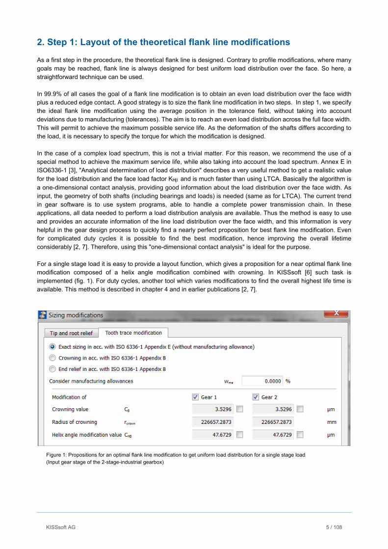
a one-dimensional contact analysis, providing good information about the load distribution over the face width. As input, the geometry of both shafts (including bearings and loads) is needed (same as for LTCA). The current trend in gear software is to use system programs, able to handle a complete power transmission chain. In these applications, all data needed to perform a load distribution analysis are available. Thus the method is easy to use and provides an accurate information of the line load distribution over the face width, and this information is very helpful in the gear design process to quickly find a nearly perfect proposition for best flank line modification. Even for complicated duty cycles it is possible to find the best modification, hence improving the overall lifetime considerably [2, 7]. Therefore, using this "one-dimensional contact analysis" is ideal for the purpose. For a single stage load it is easy to provide a layout function, which gives a proposition for a near optimal flank line modification composed of a helix angle modification combined with crowning. In KISSsoft [6] such task is implemented (fig. 1). For duty cycles, another tool which varies modifications to find the overall highest life time is available. This method is described in chapter 4 and in earlier publications [2, 7].
Figure 1: Propositions for an optimal flank line modification to get uniform load distribution for a single stage load (Input gear stage of the 2-stage-industrial gearbox)
KISSsoft AG 6 / 108
3. Step 2: Including flank line manufacturing tolerances
Once the flank line modification for the medium tolerance position is determined in step 1, the manufacturing deviations, respectively the manufacturing tolerances, must be considered. In gear modification layout normally two main tolerances are used:
Helix slope tolerance fHof the gears (for example according ISO 1328 [8]) Axis alignment tolerances f,f (parallelism of the shafts, ISO TR 10064) (f: Deviation error of axis; f: Inclination error of axis)
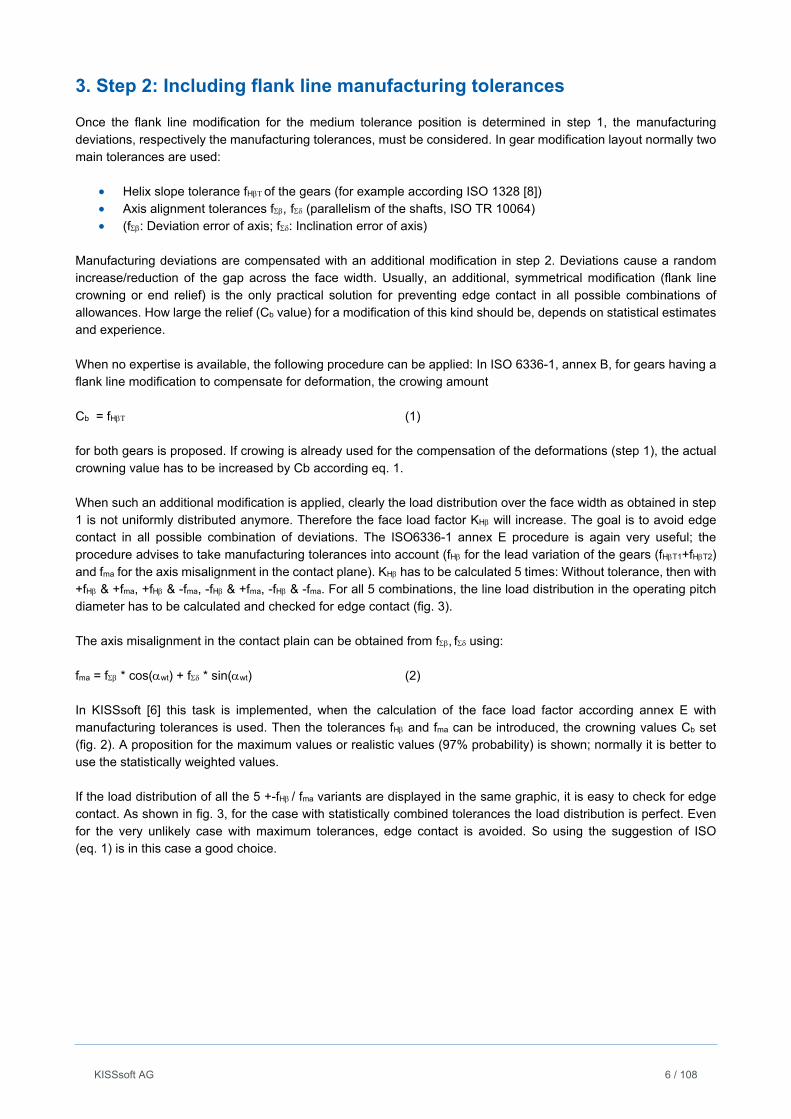
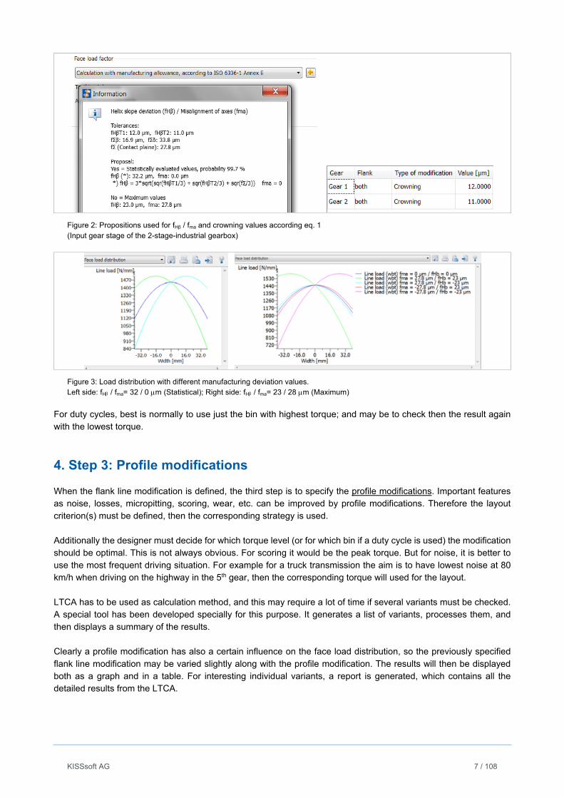
Manufacturing deviations are compensated with an additional modification in step 2. Deviations cause a random increase/reduction of the gap across the face width. Usually, an additional, symmetrical modification (flank line crowning or end relief) is the only practical solution for preventing edge contact in all possible combinations of allowances. How large the relief (Cb value) for a modification of this kind should be, depends on statistical estimates and experience. When no expertise is available, the following procedure can be applied: In ISO 6336-1, annex B, for gears having a flank line modification to compensate for deformation, the crowing amount Cb = fH (1) for both gears is proposed. If crowing is already used for the compensation of the deformations (step 1), the actual crowning value has to be increased by Cb according eq. 1. When such an additional modification is applied, clearly the load distribution over the face width as obtained in step 1 is not uniformly distributed anymore. Therefore the face load factor KH will increase. The goal is to avoid edge contact in all possible combination of deviations. The ISO6336-1 annex E procedure is again very useful; the procedure advises to take manufacturing tolerances into account (fH for the lead variation of the gears (fHT1+fHT2) and fma for the axis misalignment in the contact plane). KH has to be calculated 5 times: Without tolerance, then with +fH & +fma, +fH & -fma, -fH & +fma, -fH & -fma. For all 5 combinations, the line load distribution in the operating pitch diameter has to be calculated and checked for edge contact (fig. 3). The axis misalignment in the contact plain can be obtained from f,f using: fma = f * cos(wt) + f * sin(wt) (2) In KISSsoft [6] this task is implemented, when the calculation of the face load factor according annex E with manufacturing tolerances is used. Then the tolerances fH and fma can be introduced, the crowning values Cb set (fig. 2). A proposition for the maximum values or realistic values (97% probability) is shown; normally it is better to use the statistically weighted values. If the load distribution of all the 5 +-fH/ fma variants are displayed in the same graphic, it is easy to check for edge contact. As shown in fig. 3, for the case with statistically combined tolerances the load distribution is perfect. Even for the very unlikely case with maximum tolerances, edge contact is avoided. So using the suggestion of ISO (eq. 1) is in this case a good choice.
KISSsoft AG 7 / 108
Figure 2: Propositions used for fHβ / fma and crowning values according eq. 1 (Input gear stage of the 2-stage-industrial gearbox)
Figure 3: Load distribution with different manufacturing deviation values. Left side: fH / fma= 32 / 0 m (Statistical); Right side: fH / fma= 23 / 28 m (Maximum)
For duty cycles, best is normally to use just the bin with highest torque; and may be to check then the result again with the lowest torque.
4. Step 3: Profile modifications
When the flank line modification is defined, the third step is to specify the profile modifications. Important features as noise, losses, micropitting, scoring, wear, etc. can be improved by profile modifications. Therefore the layout criterion(s) must be defined, then the corresponding strategy is used. Additionally the designer must decide for which torque level (or for which bin if a duty cycle is used) the modification should be optimal. This is not always obvious. For scoring it would be the peak torque. But for noise, it is better to use the most frequent driving situation. For example for a truck transmission the aim is to have lowest noise at 80 km/h when driving on the highway in the 5th gear, then the corresponding torque will used for the layout. LTCA has to be used as calculation method, and this may require a lot of time if several variants must be checked. A special tool has been developed specially for this purpose. It generates a list of variants, processes them, and then displays a summary of the results. Clearly a profile modification has also a certain influence on the face load distribution, so the previously specified flank line modification may be varied slightly along with the profile modification. The results will then be displayed both as a graph and in a table. For interesting individual variants, a report is generated, which contains all the detailed results from the LTCA.
KISSsoft AG 8 / 108
Layout for low-noise
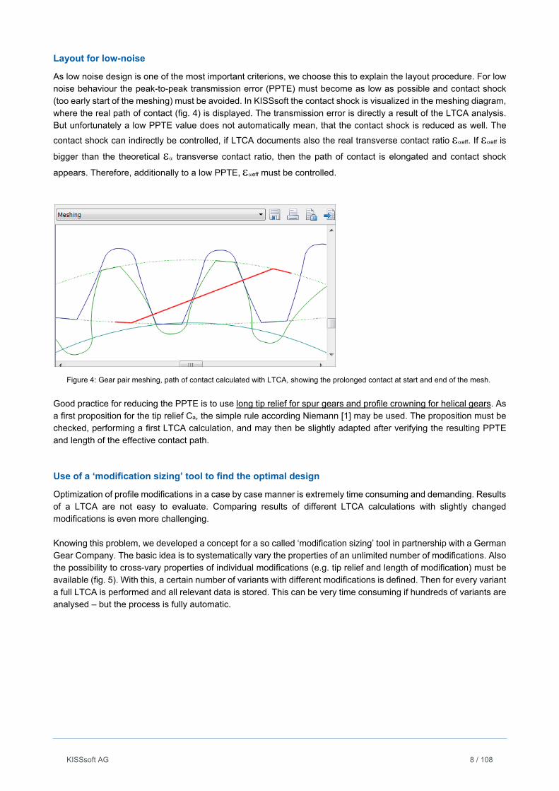
As low noise design is one of the most important criterions, we choose this to explain the layout procedure. For low noise behaviour the peak-to-peak transmission error (PPTE) must become as low as possible and contact shock (too early start of the meshing) must be avoided. In KISSsoft the contact shock is visualized in the meshing diagram, where the real path of contact (fig. 4) is displayed. The transmission error is directly a result of the LTCA analysis. But unfortunately a low PPTE value does not automatically mean, that the contact shock is reduced as well. The
contact shock can indirectly be controlled, if LTCA documents also the real transverse contact ratio eff. If eff is
bigger than the theoretical transverse contact ratio, then the path of contact is elongated and contact shock
appears. Therefore, additionally to a low PPTE, eff must be controlled.
Figure 4: Gear pair meshing, path of contact calculated with LTCA, showing the prolonged contact at start and end of the mesh.
Good practice for reducing the PPTE is to use long tip relief for spur gears and profile crowning for helical gears. As a first proposition for the tip relief Ca, the simple rule according Niemann [1] may be used. The proposition must be checked, performing a first LTCA calculation, and may then be slightly adapted after verifying the resulting PPTE and length of the effective contact path.
Use of a ‘modification sizing’ tool to find the optimal design
Optimization of profile modifications in a case by case manner is extremely time consuming and demanding. Results of a LTCA are not easy to evaluate. Comparing results of different LTCA calculations with slightly changed modifications is even more challenging. Knowing this problem, we developed a concept for a so called ‘modification sizing’ tool in partnership with a German Gear Company. The basic idea is to systematically vary the properties of an unlimited number of modifications. Also the possibility to cross-vary properties of individual modifications (e.g. tip relief and length of modification) must be available (fig. 5). With this, a certain number of variants with different modifications is defined. Then for every variant a full LTCA is performed and all relevant data is stored. This can be very time consuming if hundreds of variants are analysed – but the process is fully automatic.
KISSsoft AG 9 / 108
Tab. I: Contains all modifications which will not be changed
Tab. II: Definition of modifications which will be varied
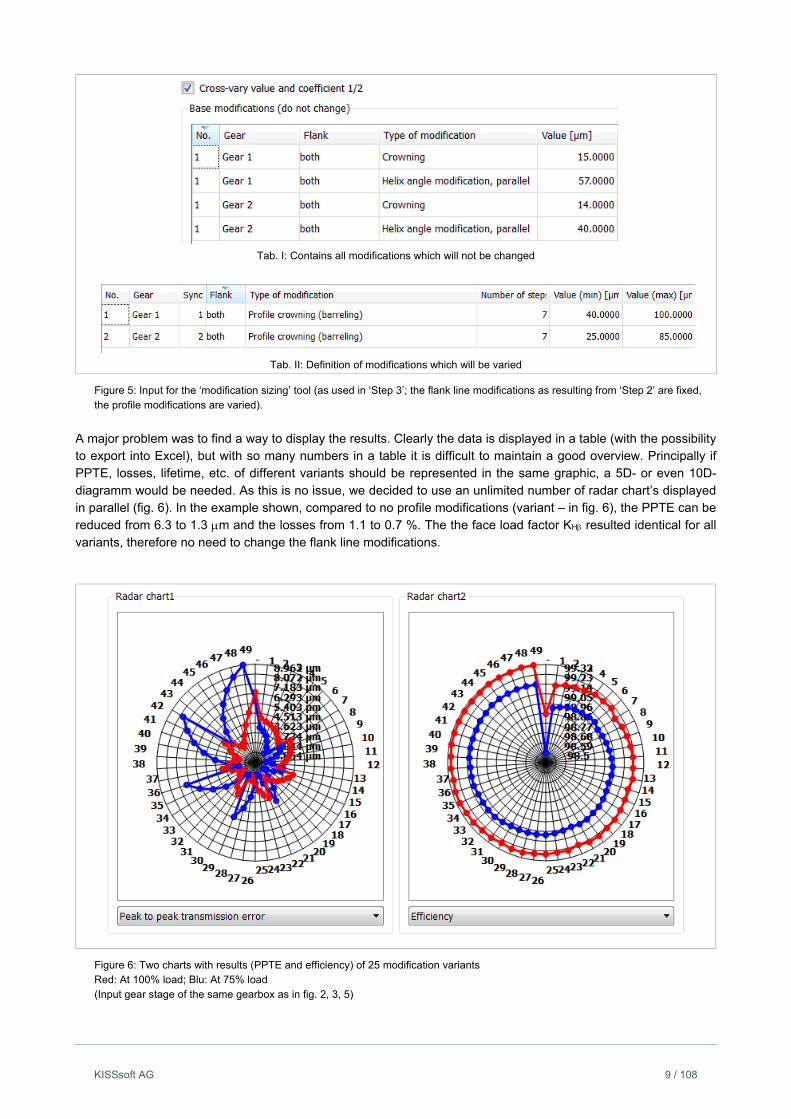
Figure 5: Input for the ‘modification sizing’ tool (as used in ‘Step 3’; the flank line modifications as resulting from ‘Step 2’ are fixed, the profile modifications are varied).
A major problem was to find a way to display the results. Clearly the data is displayed in a table (with the possibility to export into Excel), but with so many numbers in a table it is difficult to maintain a good overview. Principally if PPTE, losses, lifetime, etc. of different variants should be represented in the same graphic, a 5D- or even 10D-diagramm would be needed. As this is no issue, we decided to use an unlimited number of radar chart’s displayed in parallel (fig. 6). In the example shown, compared to no profile modifications (variant – in fig. 6), the PPTE can be reduced from 6.3 to 1.3 m and the losses from 1.1 to 0.7 %. The the face load factor KH resulted identical for all variants, therefore no need to change the flank line modifications.
Figure 6: Two charts with results (PPTE and efficiency) of 25 modification variants Red: At 100% load; Blu: At 75% load (Input gear stage of the same gearbox as in fig. 2, 3, 5)
KISSsoft AG 10 / 108
5. Considering housing and/or planet carrier stiffness
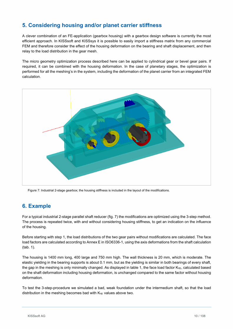
A clever combination of an FE-application (gearbox housing) with a gearbox design software is currently the most efficient approach. In KISSsoft and KISSsys it is possible to easily import a stiffness matrix from any commercial FEM and therefore consider the effect of the housing deformation on the bearing and shaft displacement, and then relay to the load distribution in the gear mesh. The micro geometry optimization process described here can be applied to cylindrical gear or bevel gear pairs. If required, it can be combined with the housing deformation. In the case of planetary stages, the optimization is performed for all the meshing’s in the system, including the deformation of the planet carrier from an integrated FEM calculation.
Figure 7: Industrial 2-stage gearbox; the housing stiffness is included in the layout of the modifications.
6. Example
For a typical industrial 2-stage parallel shaft reducer (fig. 7) the modifications are optimized using the 3-step method. The process is repeated twice, with and without considering housing stiffness, to get an indication on the influence of the housing. Before starting with step 1, the load distributions of the two gear pairs without modifications are calculated. The face load factors are calculated according to Annex E in ISO6336-1, using the axis deformations from the shaft calculation (tab. 1). The housing is 1400 mm long, 400 large and 750 mm high. The wall thickness is 20 mm, which is moderate. The elastic yielding in the bearing supports is about 0.1 mm, but as the yielding is similar in both bearings of every shaft, the gap in the meshing is only minimally changed. As displayed in table 1, the face load factor KH, calculated based on the shaft deformation including housing deformation, is unchanged compared to the same factor without housing deformation. To test the 3-step-procedure we simulated a bad, weak foundation under the intermedium shaft, so that the load distribution in the meshing becomes bad with KH values above two.
KISSsoft AG 11 / 108
Gear Pair KH Without housing deformation
KHWith housing deformation
Good foundation Extremely bad foundation
HSS (High speed stage) 1.166 1.667 2.320
HSS (Low speed stage) 1.299 1.306 2.410
Table 1: Face load factors without flank line modifications
6.1 Without housing stiffness
6.1.1 Step 1
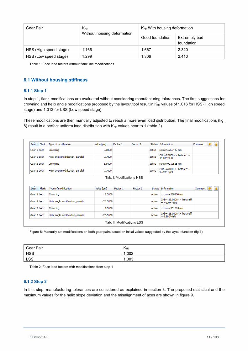
In step 1, flank modifications are evaluated without considering manufacturing tolerances. The first suggestions for crowning and helix angle modifications proposed by the layout tool result in KH values of 1.016 for HSS (High speed stage) and 1.012 for LSS (Low speed stage). These modifications are then manually adjusted to reach a more even load distribution. The final modifications (fig. 8) result in a perfect uniform load distribution with KH values near to 1 (table 2).
Tab. I: Modifications HSS
Tab. II: Modifications LSS
Figure 8: Manually set modifications on both gear pairs based on initial values suggested by the layout function (fig.1)
Gear Pair KH HSS 1.002
LSS 1.003
Table 2: Face load factors with modifications from step 1
6.1.2 Step 2
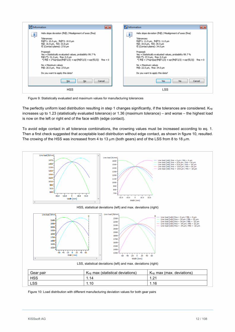
In this step, manufacturing tolerances are considered as explained in section 3. The proposed statistical and the maximum values for the helix slope deviation and the misalignment of axes are shown in figure 9.
KISSsoft AG 12 / 108
HSS
LSS
Figure 9: Statistically evaluated and maximum values for manufacturing tolerances
The perfectly uniform load distribution resulting in step 1 changes significantly, if the tolerances are considered. KH increases up to 1.23 (statistically evaluated tolerance) or 1.36 (maximum tolerance) – and worse – the highest load is now on the left or right end of the face width (edge contact). To avoid edge contact in all tolerance combinations, the crowning values must be increased according to eq. 1. Then a first check suggested that acceptable load distribution without edge contact, as shown in figure 10, resulted. The crowing of the HSS was increased from 4 to 13 m (both gears) and of the LSS from 8 to 18 m.
HSS, statistical deviations (left) and max. deviations (right)
LSS, statistical deviations (left) and max. deviations (right)
Gear pair KHmax (statistical deviations) KHmax (max. deviations)
HSS 1.14 1.21
LSS 1.10 1.16
Figure 10: Load distribution with different manufacturing deviation values for both gear pairs
KISSsoft AG 13 / 108
6.1.3 Step 3
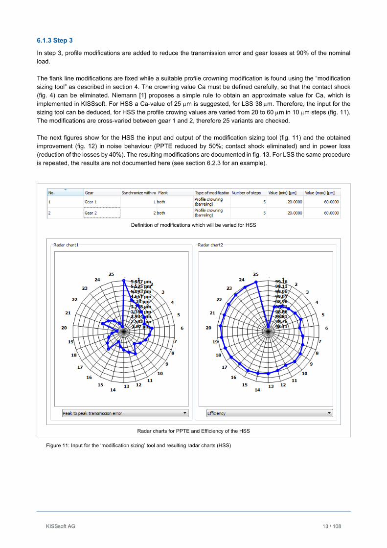
In step 3, profile modifications are added to reduce the transmission error and gear losses at 90% of the nominal load. The flank line modifications are fixed while a suitable profile crowning modification is found using the “modification sizing tool” as described in section 4. The crowning value Ca must be defined carefully, so that the contact shock (fig. 4) can be eliminated. Niemann [1] proposes a simple rule to obtain an approximate value for Ca, which is implemented in KISSsoft. For HSS a Ca-value of 25 m is suggested, for LSS 38m. Therefore, the input for the sizing tool can be deduced, for HSS the profile crowing values are varied from 20 to 60 m in 10 m steps (fig. 11). The modifications are cross-varied between gear 1 and 2, therefore 25 variants are checked. The next figures show for the HSS the input and output of the modification sizing tool (fig. 11) and the obtained improvement (fig. 12) in noise behaviour (PPTE reduced by 50%; contact shock eliminated) and in power loss (reduction of the losses by 40%). The resulting modifications are documented in fig. 13. For LSS the same procedure is repeated, the results are not documented here (see section 6.2.3 for an example).
Definition of modifications which will be varied for HSS
Radar charts for PPTE and Efficiency of the HSS
Figure 11: Input for the ‘modification sizing’ tool and resulting radar charts (HSS)
KISSsoft AG 14 / 108
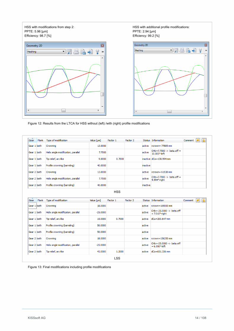
HSS with modifications from step 2: PPTE: 5.96 [µm] Efficiency: 98.7 [%]
HSS with additional profile modifications: PPTE: 2.94 [µm] Efficiency: 99.2 [%]
Figure 12: Results from the LTCA for HSS without (left) /with (right) profile modifications
HSS
LSS
Figure 13: Final modifications including profile modifications
KISSsoft AG 15 / 108
6.2 With housing stiffness
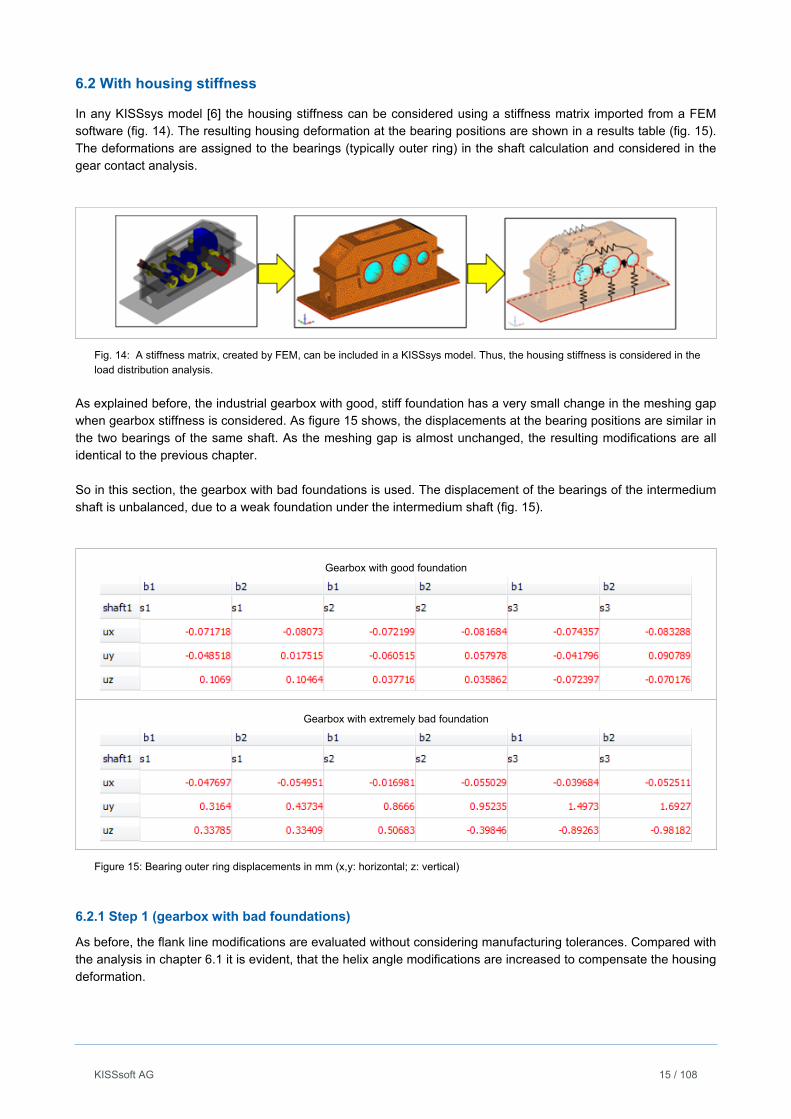
In any KISSsys model [6] the housing stiffness can be considered using a stiffness matrix imported from a FEM software (fig. 14). The resulting housing deformation at the bearing positions are shown in a results table (fig. 15). The deformations are assigned to the bearings (typically outer ring) in the shaft calculation and considered in the gear contact analysis.
Fig. 14: A stiffness matrix, created by FEM, can be included in a KISSsys model. Thus, the housing stiffness is considered in the load distribution analysis.
As explained before, the industrial gearbox with good, stiff foundation has a very small change in the meshing gap when gearbox stiffness is considered. As figure 15 shows, the displacements at the bearing positions are similar in the two bearings of the same shaft. As the meshing gap is almost unchanged, the resulting modifications are all identical to the previous chapter. So in this section, the gearbox with bad foundations is used. The displacement of the bearings of the intermedium shaft is unbalanced, due to a weak foundation under the intermedium shaft (fig. 15).
Gearbox with good foundation
Gearbox with extremely bad foundation
Figure 15: Bearing outer ring displacements in mm (x,y: horizontal; z: vertical)
6.2.1 Step 1 (gearbox with bad foundations)
As before, the flank line modifications are evaluated without considering manufacturing tolerances. Compared with the analysis in chapter 6.1 it is evident, that the helix angle modifications are increased to compensate the housing deformation.
KISSsoft AG 16 / 108
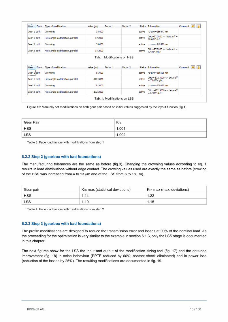
Tab. I: Modifications on HSS
Tab. II: Modifications on LSS
Figure 16: Manually set modifications on both gear pair based on initial values suggested by the layout function (fig.1)
Gear Pair KH
HSS 1.001
LSS 1.002
Table 3: Face load factors with modifications from step 1
6.2.2 Step 2 (gearbox with bad foundations)
The manufacturing tolerances are the same as before (fig.9). Changing the crowning values according to eq. 1 results in load distributions without edge contact. The crowing values used are exactly the same as before (crowing of the HSS was increased from 4 to 13 m and of the LSS from 8 to 18 m).
Gear pair KHmax (statistical deviations) KHmax (max. deviations)
HSS 1.14 1.22
LSS 1.10 1.15
Table 4: Face load factors with modifications from step 2
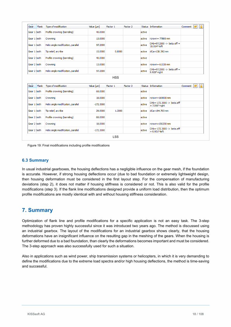
6.2.3 Step 3 (gearbox with bad foundations)
The profile modifications are designed to reduce the transmission error and losses at 90% of the nominal load. As the proceeding for the optimization is very similar to the example in section 6.1.3, only the LSS stage is documented in this chapter. The next figures show for the LSS the input and output of the modification sizing tool (fig. 17) and the obtained improvement (fig. 18) in noise behaviour (PPTE reduced by 60%; contact shock eliminated) and in power loss (reduction of the losses by 25%). The resulting modifications are documented in fig. 19.
KISSsoft AG 17 / 108
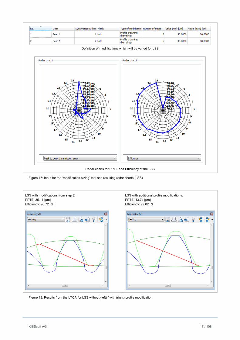
Definition of modifications which will be varied for LSS
Radar charts for PPTE and Efficiency of the LSS
Figure 17: Input for the ‘modification sizing’ tool and resulting radar charts (LSS)
LSS with modifications from step 2: PPTE: 35.11 [µm] Efficiency: 98.72 [%]
LSS with additional profile modifications: PPTE: 13.74 [µm] Efficiency: 99.02 [%]
Figure 18: Results from the LTCA for LSS without (left) / with (right) profile modification
KISSsoft AG 18 / 108
HSS
LSS
Figure 19: Final modifications including profile modifications
6.3 Summary
In usual industrial gearboxes, the housing deflections has a negligible influence on the gear mesh, if the foundation is accurate. However, if strong housing deflections occur (due to bad foundation or extremely lightweight design, then housing deformation must be considered in the first layout step. For the compensation of manufacturing deviations (step 2), it does not matter if housing stiffness is considered or not. This is also valid for the profile modifications (step 3). If the flank line modifications designed provide a uniform load distribution, then the optimum profile modifications are mostly identical with and without housing stiffness consideration.
7. Summary
Optimization of flank line and profile modifications for a specific application is not an easy task. The 3-step methodology has proven highly successful since it was introduced two years ago. The method is discussed using an industrial gearbox. The layout of the modifications for an industrial gearbox shows clearly, that the housing deformations have an insignificant influence on the resulting gap in the meshing of the gears. When the housing is further deformed due to a bad foundation, than clearly the deformations becomes important and must be considered. The 3-step approach was also successfully used for such a situation. Also in applications such as wind power, ship transmission systems or helicopters, in which it is very demanding to define the modifications due to the extreme load spectra and/or high housing deflections, the method is time-saving and successful.
KISSsoft AG 19 / 108
8. Literature
[1] Niemann, „Maschinenelemente“, Band II, Springer Verlag, 1985
[2] U. Kissling, „Auslegung optimaler Flankenkorrekturen für Stirnradpaare und Planetenstufen mit komplexen Lastkollektiven“, DMK 2013, S.67, ISBN978-3-944331-33-1. (Or: „Flankenlinienkorrekturen per Software – eine Fallstudie“; antriebstechnik 11/2013, antriebstechnik 12/2013.)
[3] ISO 6336, Part 1, „Calculation of load capacity of spur and helical gears“, ISO Geneva, 2006
[4] Bae, I; Kissling, U.; An Advanced Design Concept of Incorporating Transmission Error Calculation into a Gear Pair Optimization Procedure; International VDI conference, Munich, 2010
[5] Mahr, B.; Kontaktanalyse; Antriebstechnik 12/2011, 2011
[6] KISSsoft; Calculation software for machine design, www.KISSsoft.AG
[7] Kissling, U.; Application and Improvement of Face Load Factor Determination based on AGMA 927, AGMA Fall Technical Meeting 2013
[8] ISO 1328-1, Cylindrical gears — ISO system of flank tolerance classification, Geneva, 2013
KISSsoft AG 20 / 108
Enhanced gear efficiency calculation including contact analysis results and drive cycle consideration
Dipl.-Ing. Jürg Langhart, KISSsoft AG, Bubikon, Switzerland
M. Sc. Thomas Panéro, KISSsoft AG, Bubikon, Switzerland
Paper presented at the “International Conference on Gears 2015”
Abstract
The efficiency calculation and thermal rating for gearboxes is meanwhile a standard analysis which is requested by the customers. The basis for these calculations is the ISO/TR 14179 [1], which includes the power losses for various machine elements as well as the heat dissipation calculation. For the gear meshing losses, the formulas from ISO/TR 14179 are established but the problem remains that no flank modification are considered in these calculation. Also a known issue is the inaccuracy in the losses of oil splashing (churning losses) and other lubrication depending effects. These losses require some correction factors which let the losses adjust based on preceding measurements. These enhanced calculations are applied in KISSsys and make it capable to consider these effects on a system level. Furthermore, the consideration of a drive cycle allows the user to obtain the maximum operating temperature and also the critical load bin for the thermal stress. Additionally when the drive cycle is given the temporal temperature profile is calculated and the critical parts of the drive cycle are determined, together with the temporal losses.
Thermal rating in KISSsys
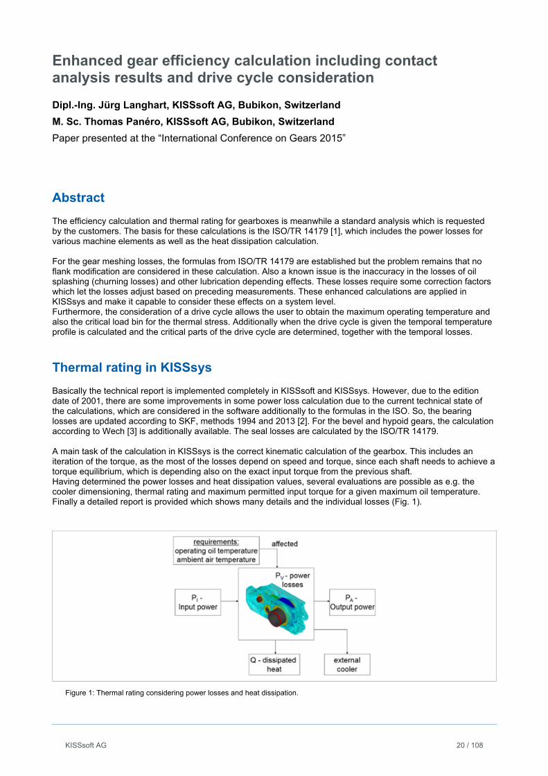
Basically the technical report is implemented completely in KISSsoft and KISSsys. However, due to the edition date of 2001, there are some improvements in some power loss calculation due to the current technical state of the calculations, which are considered in the software additionally to the formulas in the ISO. So, the bearing losses are updated according to SKF, methods 1994 and 2013 [2]. For the bevel and hypoid gears, the calculation according to Wech [3] is additionally available. The seal losses are calculated by the ISO/TR 14179. A main task of the calculation in KISSsys is the correct kinematic calculation of the gearbox. This includes an iteration of the torque, as the most of the losses depend on speed and torque, since each shaft needs to achieve a torque equilibrium, which is depending also on the exact input torque from the previous shaft. Having determined the power losses and heat dissipation values, several evaluations are possible as e.g. the cooler dimensioning, thermal rating and maximum permitted input torque for a given maximum oil temperature. Finally a detailed report is provided which shows many details and the individual losses (Fig. 1).
Figure 1: Thermal rating considering power losses and heat dissipation.
KISSsoft AG 21 / 108
Correction factors
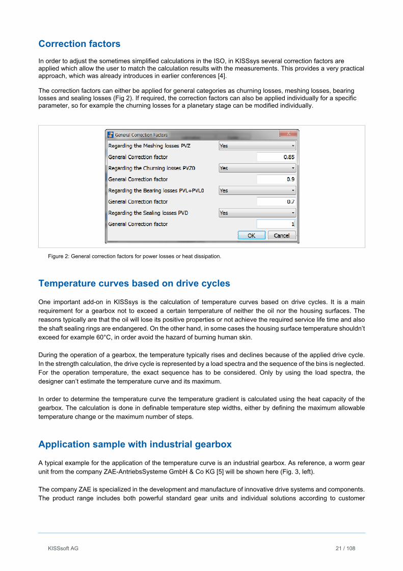
In order to adjust the sometimes simplified calculations in the ISO, in KISSsys several correction factors are applied which allow the user to match the calculation results with the measurements. This provides a very practical approach, which was already introduces in earlier conferences [4]. The correction factors can either be applied for general categories as churning losses, meshing losses, bearing losses and sealing losses (Fig 2). If required, the correction factors can also be applied individually for a specific parameter, so for example the churning losses for a planetary stage can be modified individually.
Figure 2: General correction factors for power losses or heat dissipation.
Temperature curves based on drive cycles
One important add-on in KISSsys is the calculation of temperature curves based on drive cycles. It is a main requirement for a gearbox not to exceed a certain temperature of neither the oil nor the housing surfaces. The reasons typically are that the oil will lose its positive properties or not achieve the required service life time and also the shaft sealing rings are endangered. On the other hand, in some cases the housing surface temperature shouldn’t exceed for example 60°C, in order avoid the hazard of burning human skin. During the operation of a gearbox, the temperature typically rises and declines because of the applied drive cycle. In the strength calculation, the drive cycle is represented by a load spectra and the sequence of the bins is neglected. For the operation temperature, the exact sequence has to be considered. Only by using the load spectra, the designer can’t estimate the temperature curve and its maximum. In order to determine the temperature curve the temperature gradient is calculated using the heat capacity of the gearbox. The calculation is done in definable temperature step widths, either by defining the maximum allowable temperature change or the maximum number of steps.
Application sample with industrial gearbox
A typical example for the application of the temperature curve is an industrial gearbox. As reference, a worm gear unit from the company ZAE-AntriebsSysteme GmbH & Co KG [5] will be shown here (Fig. 3, left). The company ZAE is specialized in the development and manufacture of innovative drive systems and components. The product range includes both powerful standard gear units and individual solutions according to customer
KISSsoft AG 22 / 108
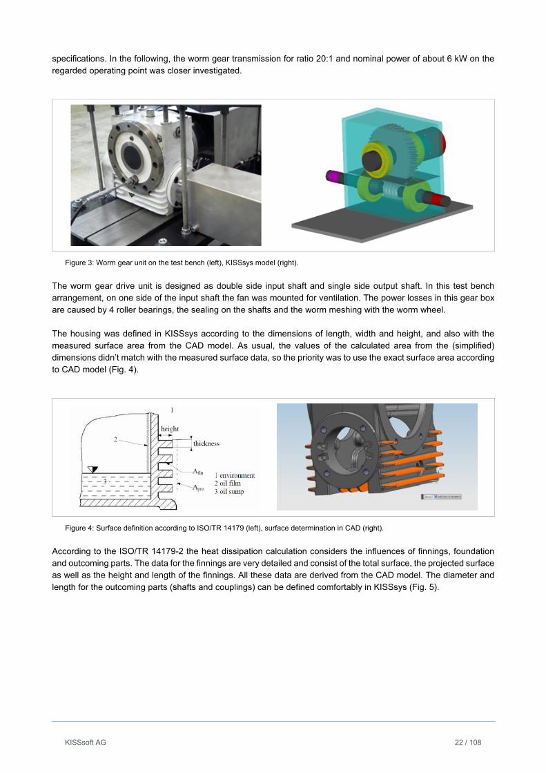
specifications. In the following, the worm gear transmission for ratio 20:1 and nominal power of about 6 kW on the regarded operating point was closer investigated.
Figure 3: Worm gear unit on the test bench (left), KISSsys model (right).
The worm gear drive unit is designed as double side input shaft and single side output shaft. In this test bench arrangement, on one side of the input shaft the fan was mounted for ventilation. The power losses in this gear box are caused by 4 roller bearings, the sealing on the shafts and the worm meshing with the worm wheel. The housing was defined in KISSsys according to the dimensions of length, width and height, and also with the measured surface area from the CAD model. As usual, the values of the calculated area from the (simplified) dimensions didn’t match with the measured surface data, so the priority was to use the exact surface area according to CAD model (Fig. 4).
Figure 4: Surface definition according to ISO/TR 14179 (left), surface determination in CAD (right).
According to the ISO/TR 14179-2 the heat dissipation calculation considers the influences of finnings, foundation and outcoming parts. The data for the finnings are very detailed and consist of the total surface, the projected surface as well as the height and length of the finnings. All these data are derived from the CAD model. The diameter and length for the outcoming parts (shafts and couplings) can be defined comfortably in KISSsys (Fig. 5).
KISSsoft AG 23 / 108
Figure 5: Automatic definition of shaft and coupling diameter and length in KISSsys.
The foundation is defined according to its real dimensions and as ‘heat transfer up- and downwards’. The ventilation speed is 1.4 m/s, as the speed of the input shaft is 1000 rpm and the diameter of the fan is 163 mm. Two important parameters for the heat dissipation are the heat transfer coefficient k* and the emission ratio ε. The heat transfer coefficient k* is either calculated by the ISO or defined by own input. The emission ratio ε is the ratio between oil and housing temperature. As a first approach, the heat transfer coefficient k* was used as calculated value, and the emission ratio ε was defined as 1.
Adaption of heat dissipation by using correction factors
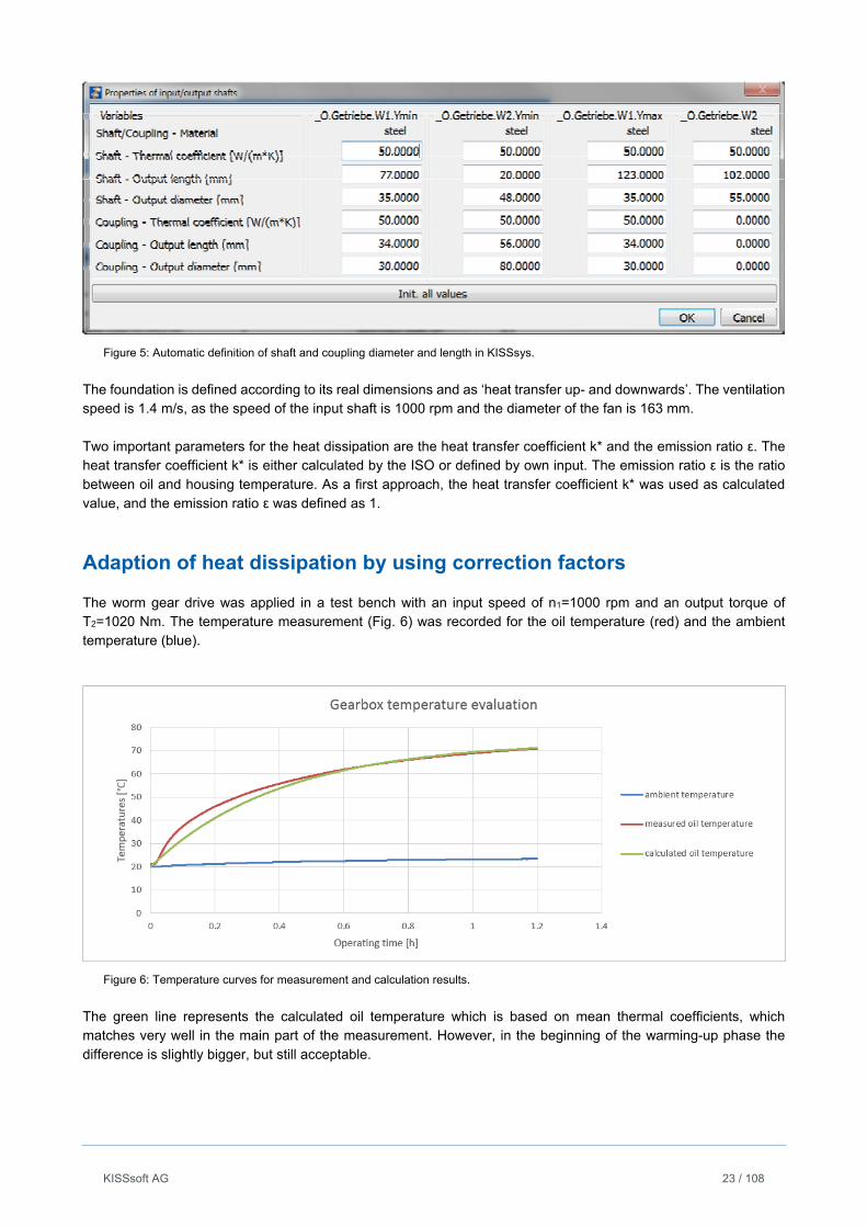
The worm gear drive was applied in a test bench with an input speed of n1=1000 rpm and an output torque of T2=1020 Nm. The temperature measurement (Fig. 6) was recorded for the oil temperature (red) and the ambient temperature (blue).
Figure 6: Temperature curves for measurement and calculation results.
The green line represents the calculated oil temperature which is based on mean thermal coefficients, which matches very well in the main part of the measurement. However, in the beginning of the warming-up phase the difference is slightly bigger, but still acceptable.
KISSsoft AG 24 / 108
The figure 7 below shows the results of the calculation and the measurements. The first temperature calculations using the calculated k* = 36 W/m2K and the emmision ratio ε = 1 were deviating by max. 4K. Using optimized values for k* = 40.9 W/m2K and emmision ratio ε = 0.925, the correlation between measurement and calculation matches within 1K, which is a very good basis for further calculations. The power losses were not modified in this case.
Figure 7: Comparison of KISSsys calculation to the measurement of the test bench.
Drive cycle and temperature curve
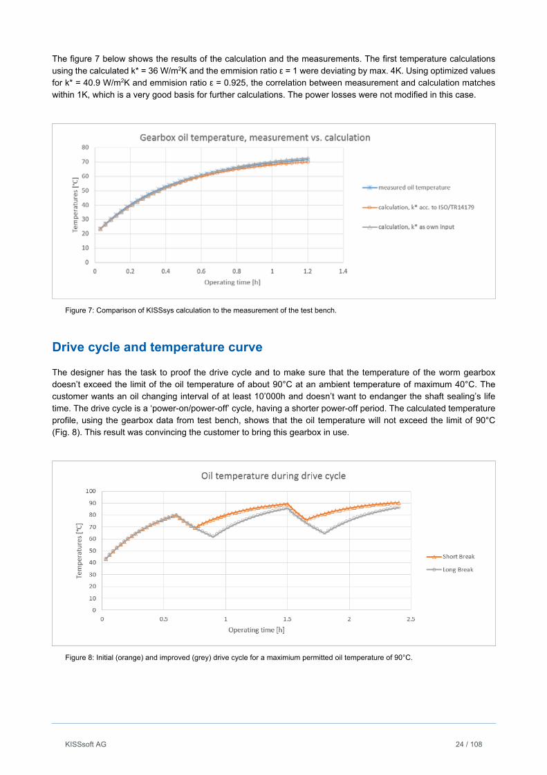
The designer has the task to proof the drive cycle and to make sure that the temperature of the worm gearbox doesn’t exceed the limit of the oil temperature of about 90°C at an ambient temperature of maximum 40°C. The customer wants an oil changing interval of at least 10’000h and doesn’t want to endanger the shaft sealing’s life time. The drive cycle is a ‘power-on/power-off’ cycle, having a shorter power-off period. The calculated temperature profile, using the gearbox data from test bench, shows that the oil temperature will not exceed the limit of 90°C (Fig. 8). This result was convincing the customer to bring this gearbox in use.
Figure 8: Initial (orange) and improved (grey) drive cycle for a maximium permitted oil temperature of 90°C.
KISSsoft AG 25 / 108
Meshing losses from gear contact analysis
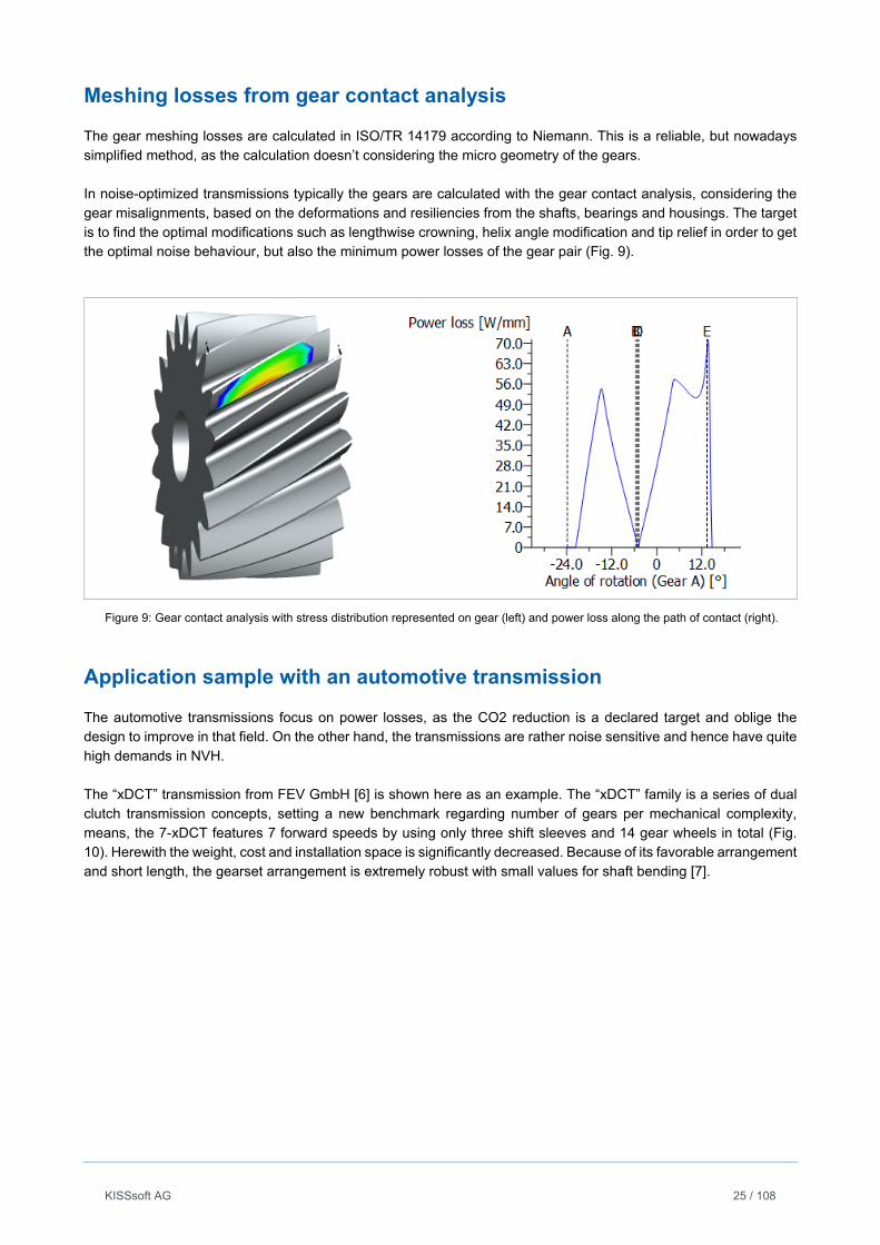
The gear meshing losses are calculated in ISO/TR 14179 according to Niemann. This is a reliable, but nowadays simplified method, as the calculation doesn’t considering the micro geometry of the gears. In noise-optimized transmissions typically the gears are calculated with the gear contact analysis, considering the gear misalignments, based on the deformations and resiliencies from the shafts, bearings and housings. The target is to find the optimal modifications such as lengthwise crowning, helix angle modification and tip relief in order to get the optimal noise behaviour, but also the minimum power losses of the gear pair (Fig. 9).
Figure 9: Gear contact analysis with stress distribution represented on gear (left) and power loss along the path of contact (right).
Application sample with an automotive transmission
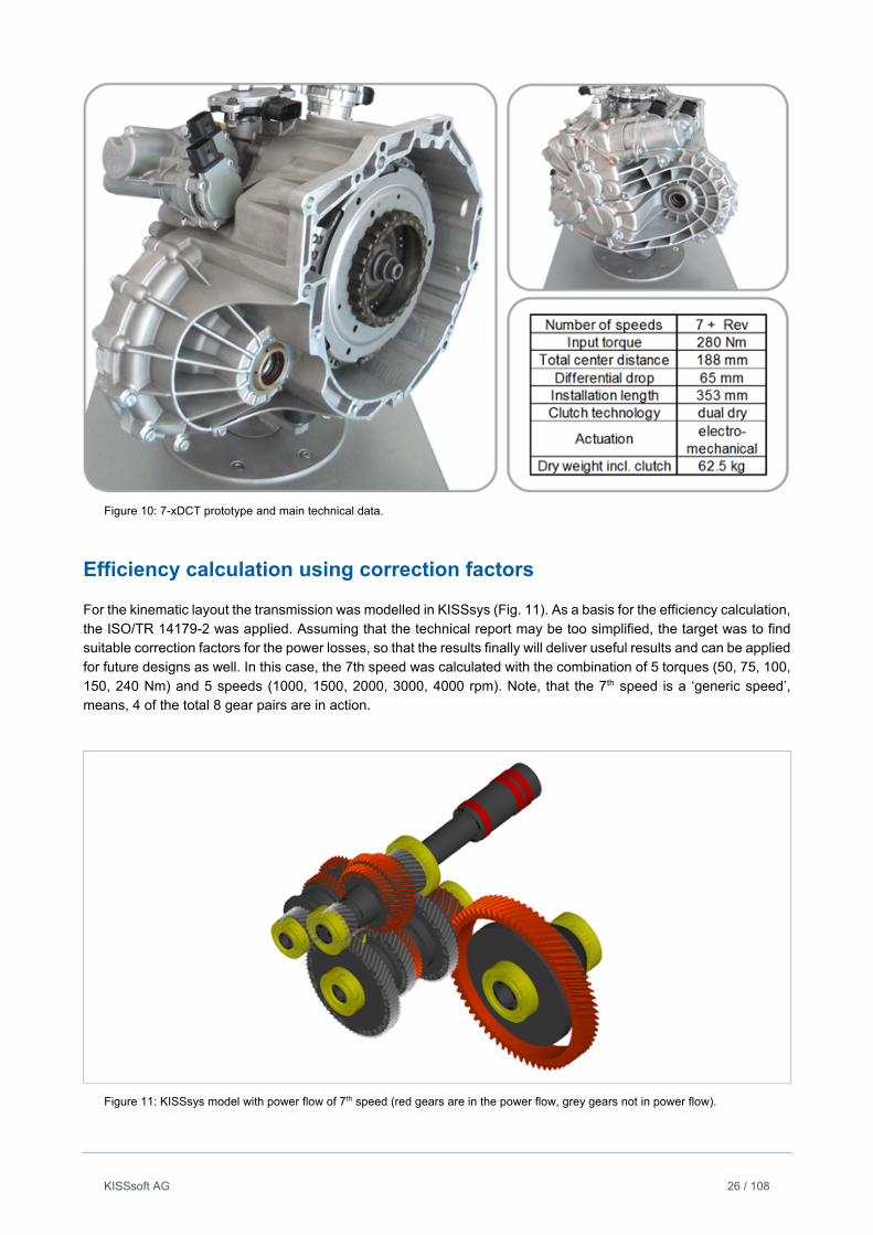
The automotive transmissions focus on power losses, as the CO2 reduction is a declared target and oblige the design to improve in that field. On the other hand, the transmissions are rather noise sensitive and hence have quite high demands in NVH. The “xDCT” transmission from FEV GmbH [6] is shown here as an example. The “xDCT” family is a series of dual clutch transmission concepts, setting a new benchmark regarding number of gears per mechanical complexity, means, the 7-xDCT features 7 forward speeds by using only three shift sleeves and 14 gear wheels in total (Fig. 10). Herewith the weight, cost and installation space is significantly decreased. Because of its favorable arrangement and short length, the gearset arrangement is extremely robust with small values for shaft bending [7].
KISSsoft AG 26 / 108
Figure 10: 7-xDCT prototype and main technical data.
Efficiency calculation using correction factors
For the kinematic layout the transmission was modelled in KISSsys (Fig. 11). As a basis for the efficiency calculation, the ISO/TR 14179-2 was applied. Assuming that the technical report may be too simplified, the target was to find suitable correction factors for the power losses, so that the results finally will deliver useful results and can be applied for future designs as well. In this case, the 7th speed was calculated with the combination of 5 torques (50, 75, 100, 150, 240 Nm) and 5 speeds (1000, 1500, 2000, 3000, 4000 rpm). Note, that the 7th speed is a ‘generic speed’, means, 4 of the total 8 gear pairs are in action.
Figure 11: KISSsys model with power flow of 7th speed (red gears are in the power flow, grey gears not in power flow).

KISSsoft AG 27 / 108
The calculated power loss values are compared to the measurements and the results are shown in the table below. In order to achieve the match of the results, the calculated results are modified by individual correction factors per speed, for gear meshing losses and churning losses. Finally, the calculation match astonishingly well with the measured data, and is capable to predict the power losses for any other speeds and similar transmission designs (Fig. 12).
Figure 12: Comparison of KISSsys calculation to the measurement of the test bench.
Looking at the correction factors, it can be found that the optimal correction factors for churning losses, they are nearly constant and obviously independent of the applied speed and torque. In contrary the optimal correction factors for the meshing losses are decreasing by approximately 20%, between speed n1=1000 rpm and n1=4000 rpm (Fig. 13).
Figure 13: Correction factors varying depending on speed.
KISSsoft AG 28 / 108
Contact analysis and gear modification sizing
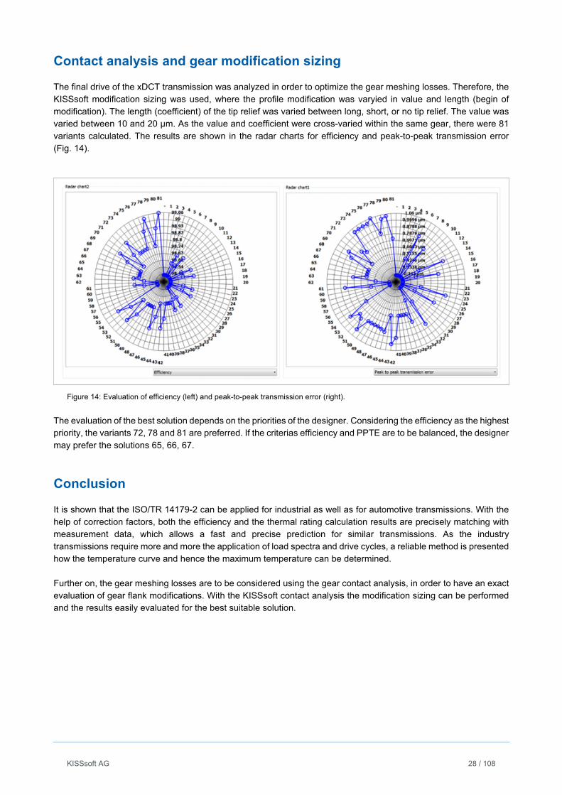
The final drive of the xDCT transmission was analyzed in order to optimize the gear meshing losses. Therefore, the KISSsoft modification sizing was used, where the profile modification was varyied in value and length (begin of modification). The length (coefficient) of the tip relief was varied between long, short, or no tip relief. The value was varied between 10 and 20 μm. As the value and coefficient were cross-varied within the same gear, there were 81 variants calculated. The results are shown in the radar charts for efficiency and peak-to-peak transmission error (Fig. 14).
Figure 14: Evaluation of efficiency (left) and peak-to-peak transmission error (right).
The evaluation of the best solution depends on the priorities of the designer. Considering the efficiency as the highest priority, the variants 72, 78 and 81 are preferred. If the criterias efficiency and PPTE are to be balanced, the designer may prefer the solutions 65, 66, 67.
Conclusion
It is shown that the ISO/TR 14179-2 can be applied for industrial as well as for automotive transmissions. With the help of correction factors, both the efficiency and the thermal rating calculation results are precisely matching with measurement data, which allows a fast and precise prediction for similar transmissions. As the industry transmissions require more and more the application of load spectra and drive cycles, a reliable method is presented how the temperature curve and hence the maximum temperature can be determined. Further on, the gear meshing losses are to be considered using the gear contact analysis, in order to have an exact evaluation of gear flank modifications. With the KISSsoft contact analysis the modification sizing can be performed and the results easily evaluated for the best suitable solution.

KISSsoft AG 29 / 108
Literature
[1] ISO/TR 14179:2001-07(E), Gears – Thermal capacity, Berlin
[2] SKF, Main Catalog, 1994 and 2013
[3] Wech, L.: Untersuchungen zum Wirkungsgrad von Kegel- und Hypoidgetrieben, Diss. TU München, 1987
[4] Langhart, J.: How to get most realistic efficiency calculation for gearboxes, International Gear conference Lyon, France, 2014
[5] Website ZAE-AntriebsSysteme GmbH & Co KG, www.zae.de, 2015
[6] Website FEV GmbH, www.fev.com, 2015
[7] Hellenbroich, G.: FEV's Extremely Compact 7-xDCT - First Test Results, 22. Aachener Kolloquium „Fahrzeug- und Motorentechnik“, 2013
KISSsoft AG 30 / 108
Combining different manufacturing errors for calculation of KHβ along ISO6336-1, Annex E
Hanspeter Dinner, Managing Director, EES KISSsoft GmbH, Switzerland
Article published in „Gear Technology“, March/April 2015
1. Introduction
Let us look at a mesh between a pinion and a gear, both situated on a shaft. The shafts in turn are supported in a housing. Then, we should consider the following three errors:
1) Helix slope deviation of the pinion, fHβ1 2) Helix slope deviation of the gear, fHβ2 3) Shaft parallelism error, fpar
Deviations 1) and 2) describe how much the flank of each gear is misaligned to the gear axis. Error 3) describes how the two gear axes are misaligned with respect to each other. This is often simplified to the gear shaft misalignment with respect to the shaft of the pinion (or vice versa). The errors are with respect to the plane of action, for a definition of the error see e.g. ISO1328 or AGMA2015.
1.1 Determining manufacturing errors
The errors fHβ1 and fHβ2 can either be measured and averaged values from production or they can be determined from the gear quality number Q, e.g. Q=6 (gear quality 6 as per ISO1328). The error fpar is more difficult to determine as it not only considers the misalignment of one shaft to the other due to the misalignment of the housing bores, but it should also consider variations in bearing operating clearances and the misalignment between of the gear pitch cylinder with respect to the corresponding shaft axis. For the sake of simplicity, let us assume the housing bore arrangement is tolerated in such a way that we know the permissible shaft or gear axes parallelism error from the manufacturing drawing.
1.2 Extreme values
All errors are considered as random and the mean is zero (e.g. tolerances given in drawing are symmetrical). The errors are hence described as a tolerance around zero, e.g. fHβ1=+-a, fHβ2=+-b and fpar=+-c where a, b, c are values in micron. Now the question is how the tolerances or permissible errors a, b, and c are to be combined for the calculation of KHβ. For the resulting misalignment we define the tolerance by the character d and find in general terms:
In a worst case scenario, the values would be added up giving a resulting misalignment
KISSsoft AG 31 / 108
However, as the errors a, b, c are random values, this approach is clearly conservative and not realistic. It is unlikely that if we combine two gears and a housing that for all three components we happen to select the worst case each. The resulting error will be overly high and will result in too high a crowning value, resulting in an unnecessary stress concentration on the flank in operation.
1.3 Random distribution
Let us assume that the manufacturing errors fHβ1, fHβ2 and fpar follow a normal distribution. As mentioned above, their mean and average value is zero. Furthermore, let us assume that 99.73% of all gears are within the specification and that also 99.73% of housings are within the specifications, or that the 3-sigma rule applies. The 3-sigma rule means that “nearly all” values are within plus minus three standard deviations from the mean value. We may translate the 3-sigma rule to the following image: If we produce a gear every day, it takes one year until one gear is out of specification. If 99.73% of all gears and housings are within the specifications (3-sigma rule applies), we know that three times the standard deviation of the manufacturing error is equal to the tolerance value a, b and c. Hence, under the assumption that 99.73% of all gears and housings are within the specified tolerance, we may define the manufacturing errors as normal distribution N with mean value μ, standard deviation σ, valid over the range of the tolerance fields defined above:
1 , ,1
√2 , 0,
3
2 , ,1
√2 , 0,
3
, ,1
√2 , 0,
3
Also, we may express the resulting error fma as a probability density function as follows
, ,1
√2 , 0,
3
Because fHβ1, fHβ2 and fpar are independent from each other, we find the standard deviation σ4 as follows:
Again assuming that 3-sigma rule applies for fma (which means that d=3*σ4) we find
3 ∗3 3 3
And
3 ∗3 3 3
This means that after assembly, 99.73% of all gearboxes have a total misalignment of the flanks with respect to each other of fma=+-d, where d is calculated as per the above formula. The above relationships are shown in the below graphic.
KISSsoft AG 32 / 108
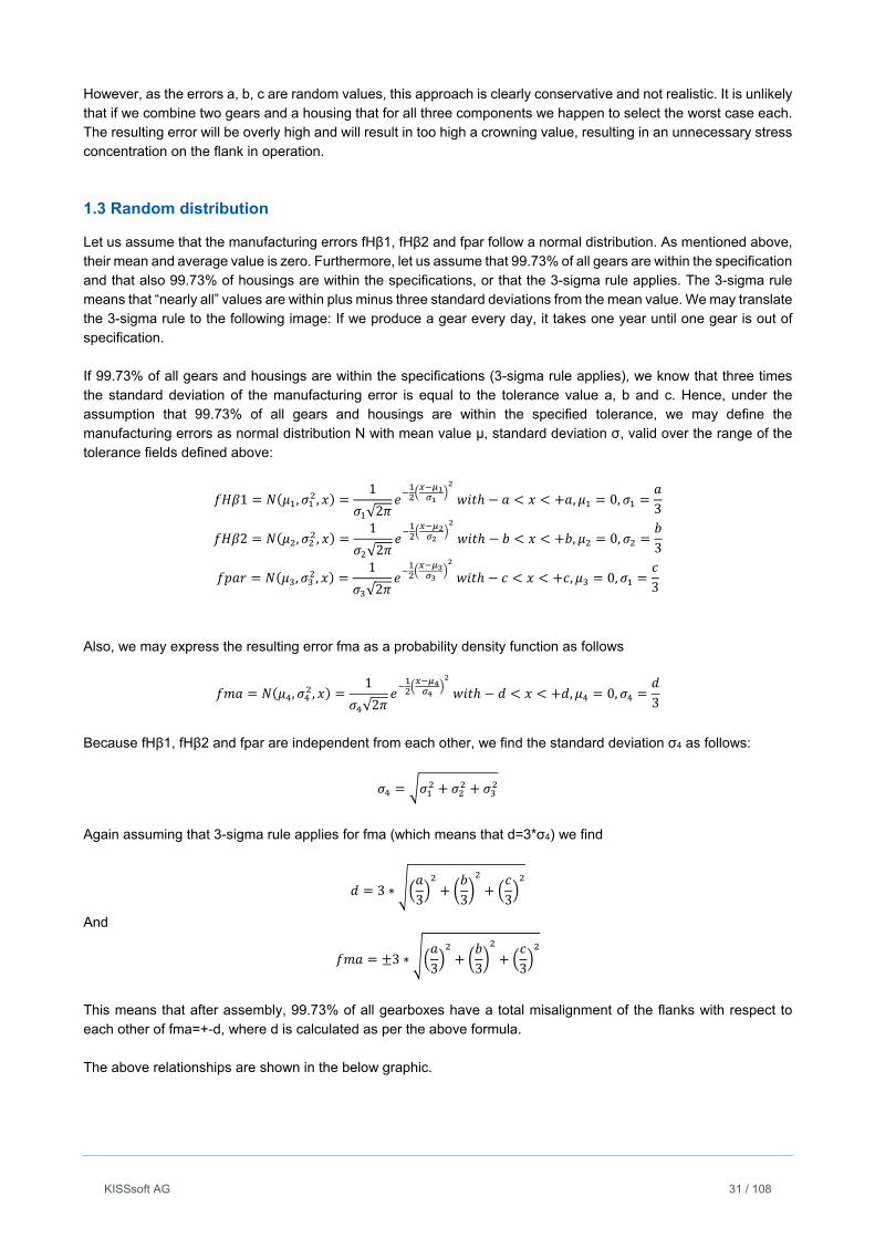
The probability density functions (assumed to be normal distributions) of the three basic errors fHβ1, fHβ2 and fpar are shown in orange, blue and black color. Also shown are the tolerances +-a, +-b, +-d corresponding to +-3*σ1, +-3*σ, +-3*σ3 (where σ is the standard deviation). Combining these three random errors we find the probability density function (again assumed to be a normal distribution) of the resulting error fma in green. Also shown is the tolerance +-d corresponding to +-3*σ4. For comparison, the worst case scenario where d=a+b+c is shown in red. We can clearly see that if we use the worst case scenario, the value for d is much higher than the value for d if we us a statistical approach.
Figure 1: Normal distribution of manufacturing errors, resulting error and worst case scenario.
2. An example
2.1 Gear data
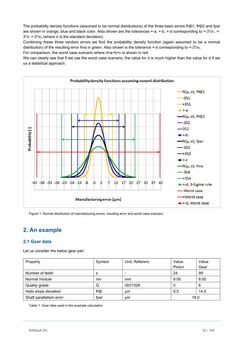
Let us consider the below gear pair:
Property Symbol Unit, Referenc Value Pinion
Value Gear
Number of teeth z - 24 99
Normal module mn mm 8.00 8.00
Quality grade Q ISO1328 5 6
Helix slope deviation fHβ μm 9.5 14.0
Shaft parallelism error fpar μm 18.0
Table 1: Gear data used in the example calculation
KISSsoft AG 33 / 108
2.2 Total misalignment
Applying the above formulas we find that the resulting tolerance range +-d if we apply 3Sigma-Rule as:
3 ∗9.50
314.0
318.0
324.7
And if we apply a worst case scenario, we find:
41.5 Considering the above statement that the worst case approach is considered as overly conservative, then, for the above gear pair, we would consider a random manufacturing error in the mesh of fma=+-d=+-24.7μm when calculating KHβ along ISO6336-1, Annex E.
2.3 KHβ calculation using statistical or worst case scenario for fma
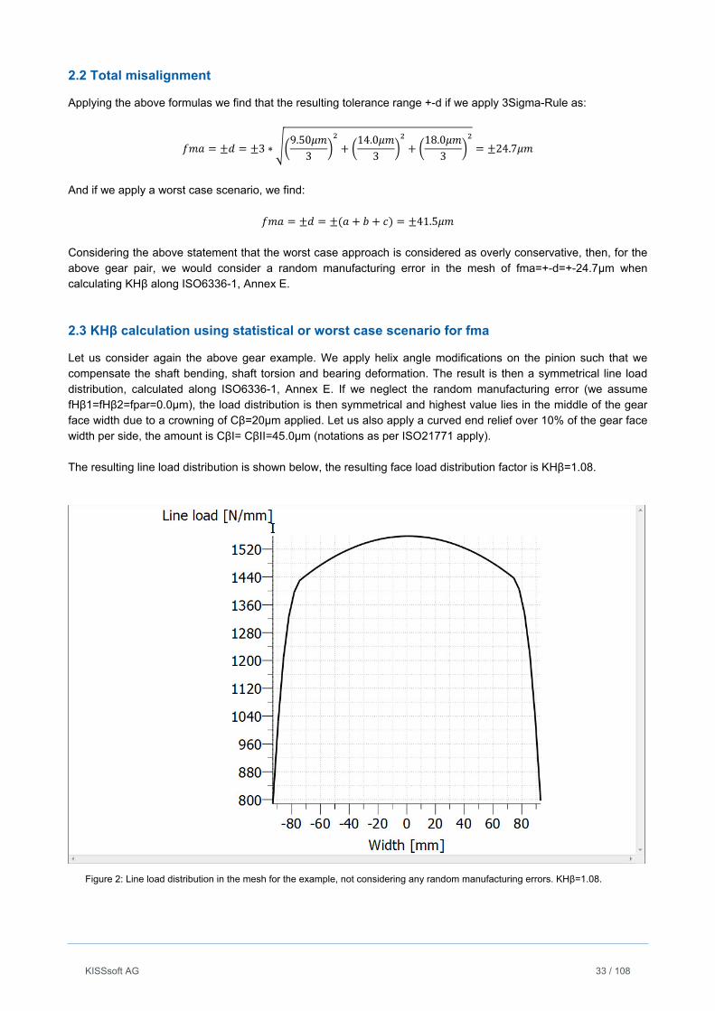
Let us consider again the above gear example. We apply helix angle modifications on the pinion such that we compensate the shaft bending, shaft torsion and bearing deformation. The result is then a symmetrical line load distribution, calculated along ISO6336-1, Annex E. If we neglect the random manufacturing error (we assume fHβ1=fHβ2=fpar=0.0μm), the load distribution is then symmetrical and highest value lies in the middle of the gear face width due to a crowning of Cβ=20μm applied. Let us also apply a curved end relief over 10% of the gear face width per side, the amount is CβI= CβII=45.0μm (notations as per ISO21771 apply). The resulting line load distribution is shown below, the resulting face load distribution factor is KHβ=1.08.
Figure 2: Line load distribution in the mesh for the example, not considering any random manufacturing errors. KHβ=1.08.
KISSsoft AG 34 / 108
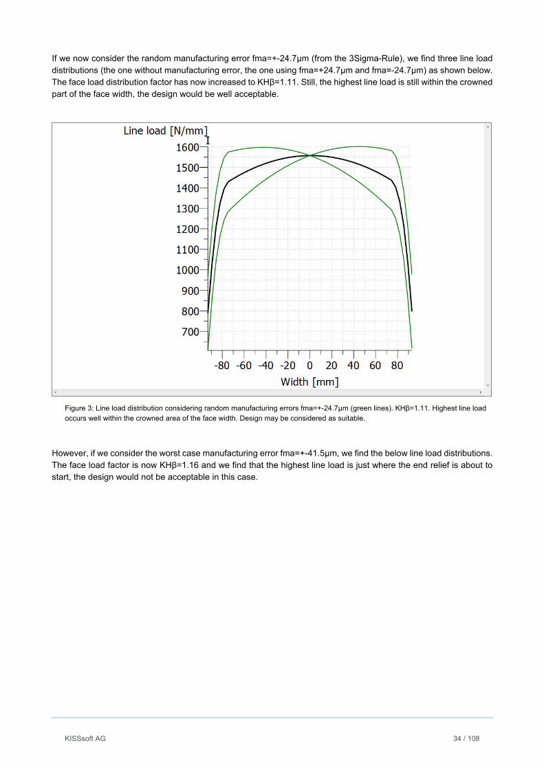
If we now consider the random manufacturing error fma=+-24.7μm (from the 3Sigma-Rule), we find three line load distributions (the one without manufacturing error, the one using fma=+24.7μm and fma=-24.7μm) as shown below. The face load distribution factor has now increased to KHβ=1.11. Still, the highest line load is still within the crowned part of the face width, the design would be well acceptable.
Figure 3: Line load distribution considering random manufacturing errors fma=+-24.7μm (green lines). KHβ=1.11. Highest line load occurs well within the crowned area of the face width. Design may be considered as suitable.
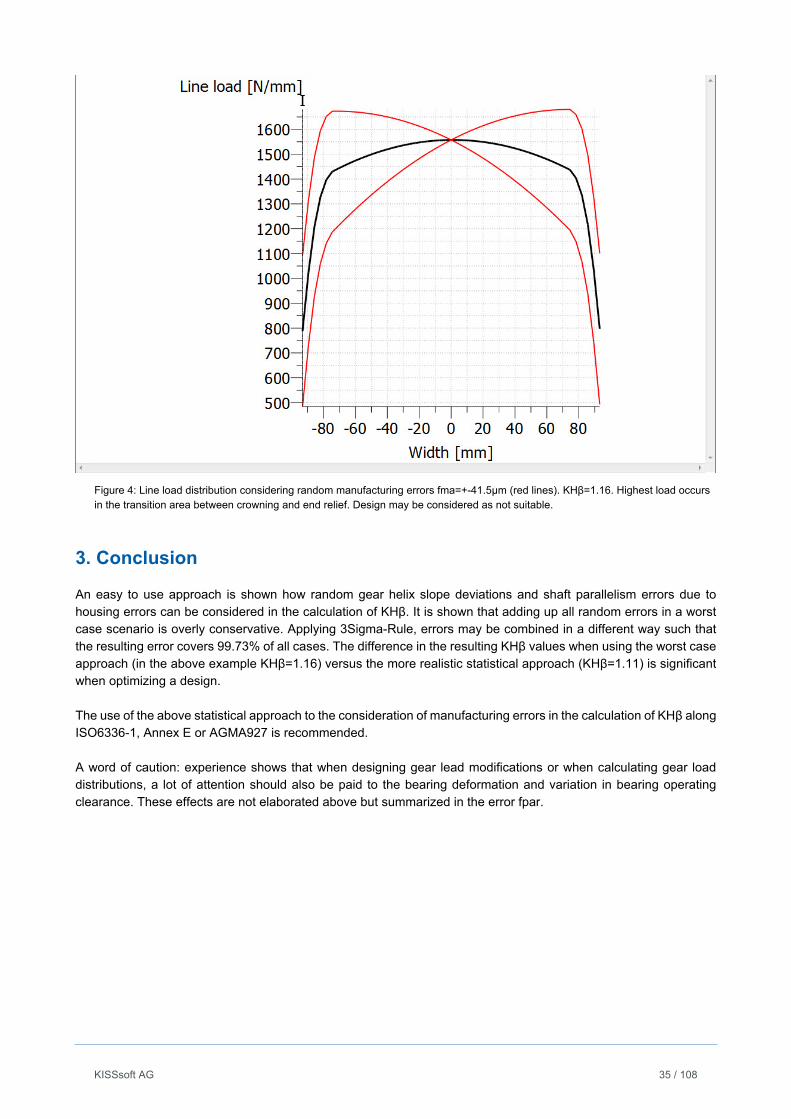
However, if we consider the worst case manufacturing error fma=+-41.5μm, we find the below line load distributions. The face load factor is now KHβ=1.16 and we find that the highest line load is just where the end relief is about to start, the design would not be acceptable in this case.
KISSsoft AG 35 / 108
Figure 4: Line load distribution considering random manufacturing errors fma=+-41.5μm (red lines). KHβ=1.16. Highest load occurs in the transition area between crowning and end relief. Design may be considered as not suitable.
3. Conclusion
An easy to use approach is shown how random gear helix slope deviations and shaft parallelism errors due to housing errors can be considered in the calculation of KHβ. It is shown that adding up all random errors in a worst case scenario is overly conservative. Applying 3Sigma-Rule, errors may be combined in a different way such that the resulting error covers 99.73% of all cases. The difference in the resulting KHβ values when using the worst case approach (in the above example KHβ=1.16) versus the more realistic statistical approach (KHβ=1.11) is significant when optimizing a design. The use of the above statistical approach to the consideration of manufacturing errors in the calculation of KHβ along ISO6336-1, Annex E or AGMA927 is recommended. A word of caution: experience shows that when designing gear lead modifications or when calculating gear load distributions, a lot of attention should also be paid to the bearing deformation and variation in bearing operating clearance. These effects are not elaborated above but summarized in the error fpar.
KISSsoft AG 36 / 108
A complete parameter study approach to designing differential bevel gears
Subtitle: Performance prediction for forged bevel gears geometries used in differentials
Dr.-Ing. A.C. Hohle, GKN Driveline International GmbH, Lohmar, Germany
Jürg Langhart, KISSsoft AG, Bubikon, Switzerland
Paper presented at the “International Conference on Gears 2015”
Abstract
Modern forged bevel gear geometries widely used in automotive differentials differ strongly from classical machined designs, which limit the accuracy of performance prediction using standard ISO calculation routines. This is mainly related to variable root radius designs, forging related tip geometries and webbing designs with varying tooth height factors at toe and heel. Through extensive testing and correlation work a simplified calculation could be obtained in the past, however leading to very different designs across car makers for the same vehicle class and general road usage. Although standard ISO tools provide some basic sizing information, they are only used to a limited extent trying to obtain “clean sheet” optimized designs with potentially higher power densities. State of the art FEA on the other hand allows better analyzing of stress distribution and correlating test results for any existing design. But due to calculation times and the necessity of exact models, this process is not feasible for a wider range parametric analysis. As part of its strategic product planning process, GKN has challenged this situation and built a project team with company KISSsoft to develop a calculation method combining the best of both worlds – fast multi-parametric variants calculation and a more accurate stress analysis for forged geometries. Following this method the macro geometry is varied by many parameters such as pressure angle, numbers of teeth, tooth heights, root and face cone angles, profile shift coefficients, tip and root radii, etc. Specific and tailored boundary conditions such as limiting contact pressure or geometric boundaries are used to reduce the huge amount of solutions to a realistic number. The strength rating itself is based on a modified ISO procedure, whilst the contact analysis is enhanced to reflect the gear shape with webbings and tip alterations and to account for the specific geometric properties influencing tooth stiffness. Micro geometry modifications with standard values are considered to determine load distribution and hence tooth bending, which results in a most realistic transmission error calculation. GKN’s ultimate goal is to find a robust optimum in bevel gear macro and micro geometry with minimized packaging for GKN AWD- and eDrive product stream applications (considering new product requirements such as special NVH performance characteristics required by AWD Booster™ disconnect drivetrains or changed durability requirements for eDrive drivetrains) to meet both performance and manufacturability constraints. Being at the heart of our components, differential sizing strongly influences system packaging from inside-out. Any benefits gained here often allow a complete downsizing of surrounding components
KISSsoft AG 37 / 108
Introduction
GKN’s ultimate goal is to find a robust optimum in bevel gear macro and micro geometry with minimized packaging for GKN’s AWD and eDrive product range whilst meeting both performance and manufacturability constraints. Minimizing packaging of differential bevel gears strongly influences system packaging from inside-out and any benefits gained here often allow a complete downsizing of surrounding components. Additional challenges are given by AWD Booster™ disconnect drivetrains, which require special NVH performance characteristics of their differential bevel gears due to their special running conditions, when disconnected or transitioning between both states connected and disconnected.
Classical vs. modern gear design and gear design process
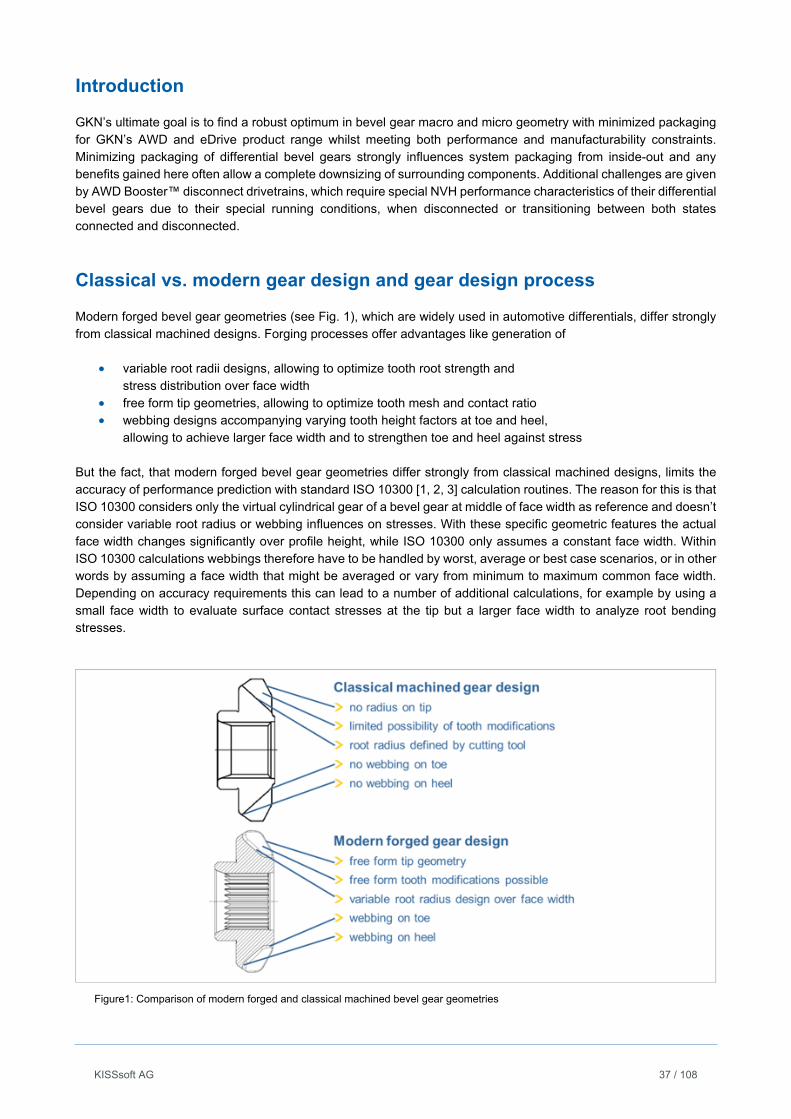
Modern forged bevel gear geometries (see Fig. 1), which are widely used in automotive differentials, differ strongly from classical machined designs. Forging processes offer advantages like generation of
variable root radii designs, allowing to optimize tooth root strength and stress distribution over face width
free form tip geometries, allowing to optimize tooth mesh and contact ratio webbing designs accompanying varying tooth height factors at toe and heel,
allowing to achieve larger face width and to strengthen toe and heel against stress But the fact, that modern forged bevel gear geometries differ strongly from classical machined designs, limits the accuracy of performance prediction with standard ISO 10300 [1, 2, 3] calculation routines. The reason for this is that ISO 10300 considers only the virtual cylindrical gear of a bevel gear at middle of face width as reference and doesn’t consider variable root radius or webbing influences on stresses. With these specific geometric features the actual face width changes significantly over profile height, while ISO 10300 only assumes a constant face width. Within ISO 10300 calculations webbings therefore have to be handled by worst, average or best case scenarios, or in other words by assuming a face width that might be averaged or vary from minimum to maximum common face width. Depending on accuracy requirements this can lead to a number of additional calculations, for example by using a small face width to evaluate surface contact stresses at the tip but a larger face width to analyze root bending stresses.
Figure1: Comparison of modern forged and classical machined bevel gear geometries
KISSsoft AG 38 / 108
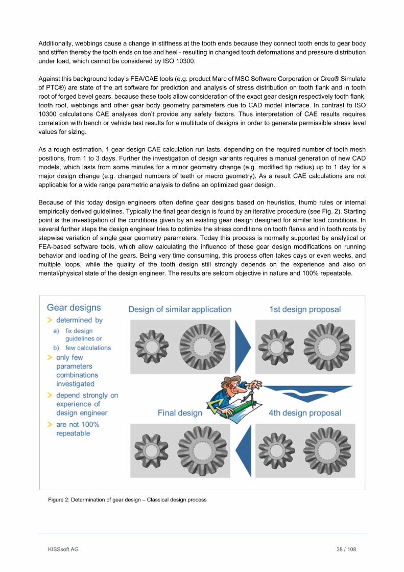
Additionally, webbings cause a change in stiffness at the tooth ends because they connect tooth ends to gear body and stiffen thereby the tooth ends on toe and heel - resulting in changed tooth deformations and pressure distribution under load, which cannot be considered by ISO 10300. Against this background today’s FEA/CAE tools (e.g. product Marc of MSC Software Corporation or Creo® Simulate of PTC®) are state of the art software for prediction and analysis of stress distribution on tooth flank and in tooth root of forged bevel gears, because these tools allow consideration of the exact gear design respectively tooth flank, tooth root, webbings and other gear body geometry parameters due to CAD model interface. In contrast to ISO 10300 calculations CAE analyses don’t provide any safety factors. Thus interpretation of CAE results requires correlation with bench or vehicle test results for a multitude of designs in order to generate permissible stress level values for sizing. As a rough estimation, 1 gear design CAE calculation run lasts, depending on the required number of tooth mesh positions, from 1 to 3 days. Further the investigation of design variants requires a manual generation of new CAD models, which lasts from some minutes for a minor geometry change (e.g. modified tip radius) up to 1 day for a major design change (e.g. changed numbers of teeth or macro geometry). As a result CAE calculations are not applicable for a wide range parametric analysis to define an optimized gear design. Because of this today design engineers often define gear designs based on heuristics, thumb rules or internal empirically derived guidelines. Typically the final gear design is found by an iterative procedure (see Fig. 2). Starting point is the investigation of the conditions given by an existing gear design designed for similar load conditions. In several further steps the design engineer tries to optimize the stress conditions on tooth flanks and in tooth roots by stepwise variation of single gear geometry parameters. Today this process is normally supported by analytical or FEA-based software tools, which allow calculating the influence of these gear design modifications on running behavior and loading of the gears. Being very time consuming, this process often takes days or even weeks, and multiple loops, while the quality of the tooth design still strongly depends on the experience and also on mental/physical state of the design engineer. The results are seldom objective in nature and 100% repeatable.
Figure 2: Determination of gear design – Classical design process
KISSsoft AG 39 / 108
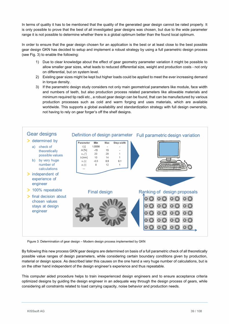
In terms of quality it has to be mentioned that the quality of the generated gear design cannot be rated properly. It is only possible to prove that the best of all investigated gear designs was chosen, but due to the wide parameter range it is not possible to determine whether there is a global optimum better than the found local optimum. In order to ensure that the gear design chosen for an application is the best or at least close to the best possible gear design GKN has decided to setup and implement a robust strategy by using a full parametric design process (see Fig. 3) to enable the following:
1) Due to clear knowledge about the effect of gear geometry parameter variation it might be possible to allow smaller gear sizes, what leads to reduced differential size, weight and production costs - not only on differential, but on system level.
2) Existing gear sizes might be kept but higher loads could be applied to meet the ever increasing demand in torque density.
3) If the parametric design study considers not only main geometrical parameters like module, face width and numbers of teeth, but also production process related parameters like allowable materials and minimum required tip radii etc., a robust gear design can be found, that can be manufactured by various production processes such as cold and warm forging and uses materials, which are available worldwide. This supports a global availability and standardization strategy with full design ownership, not having to rely on gear forger’s off the shelf designs.
Figure 3: Determination of gear design – Modern design process implemented by GKN
By following this new process GKN gear designs are determined on basis of a full parametric check of all theoretically possible value ranges of design parameters, while considering certain boundary conditions given by production, material or design space. As described later this causes on the one hand a very huge number of calculations, but is on the other hand independent of the design engineer’s experience and thus repeatable. This computer aided procedure helps to train inexperienced design engineers and to ensure acceptance criteria optimized designs by guiding the design engineer in an adequate way through the design process of gears, while considering all constraints related to load carrying capacity, noise behavior and production needs.
KISSsoft AG 40 / 108
The final decision about which parameters are to be varied, their ranges, as well as the decision/selection of final gear design stays with the design engineer. This allows rerunning the optimization procedure whenever new sets of input parameters appear on the horizon. The following describes how this was realized by GKN in cooperation with company KISSsoft.
Realized full parametric gear design process
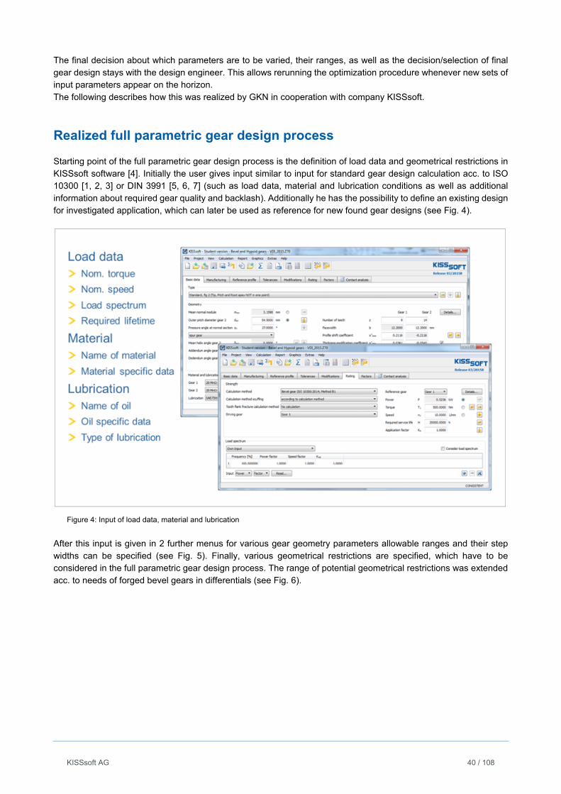
Starting point of the full parametric gear design process is the definition of load data and geometrical restrictions in KISSsoft software [4]. Initially the user gives input similar to input for standard gear design calculation acc. to ISO 10300 [1, 2, 3] or DIN 3991 [5, 6, 7] (such as load data, material and lubrication conditions as well as additional information about required gear quality and backlash). Additionally he has the possibility to define an existing design for investigated application, which can later be used as reference for new found gear designs (see Fig. 4).
Figure 4: Input of load data, material and lubrication
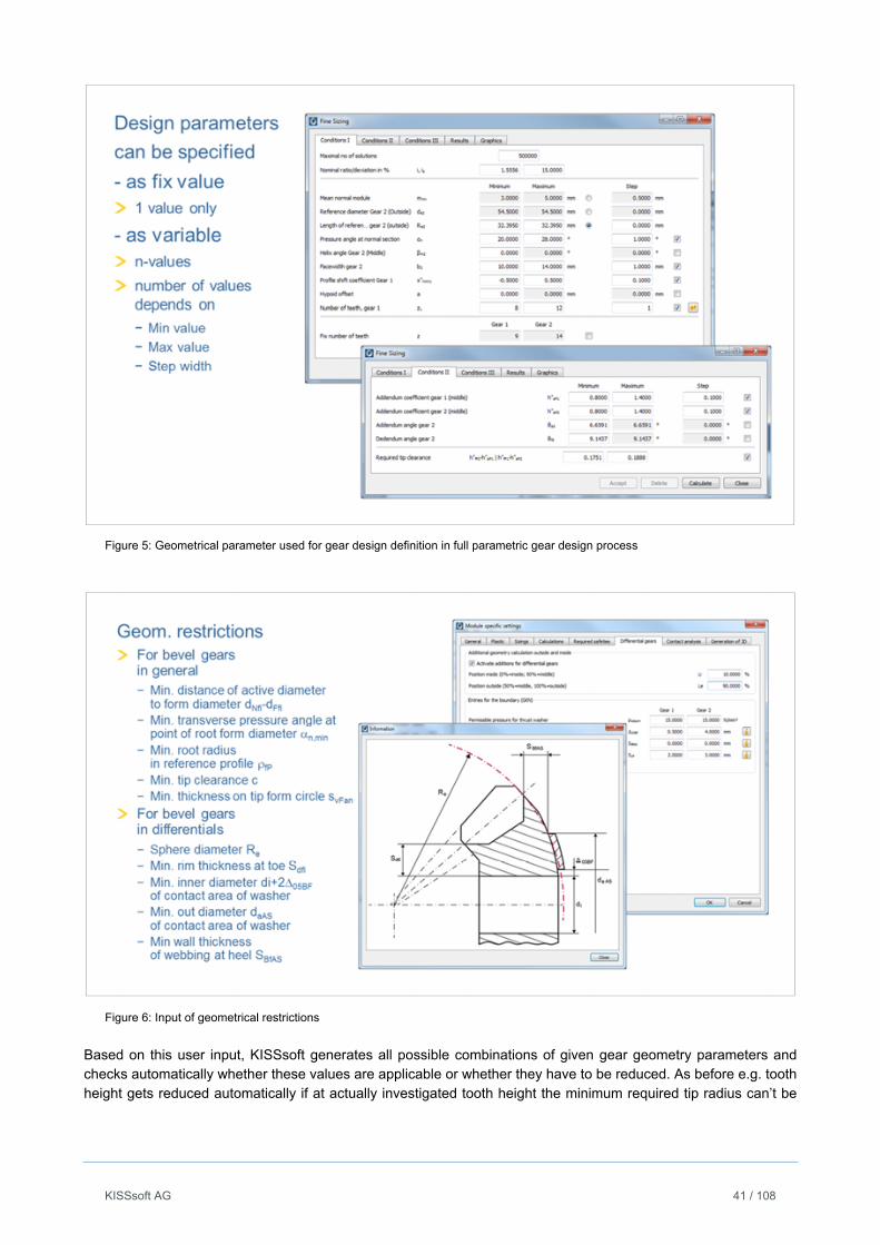
After this input is given in 2 further menus for various gear geometry parameters allowable ranges and their step widths can be specified (see Fig. 5). Finally, various geometrical restrictions are specified, which have to be considered in the full parametric gear design process. The range of potential geometrical restrictions was extended acc. to needs of forged bevel gears in differentials (see Fig. 6).
KISSsoft AG 41 / 108
Figure 5: Geometrical parameter used for gear design definition in full parametric gear design process
Figure 6: Input of geometrical restrictions
Based on this user input, KISSsoft generates all possible combinations of given gear geometry parameters and checks automatically whether these values are applicable or whether they have to be reduced. As before e.g. tooth height gets reduced automatically if at actually investigated tooth height the minimum required tip radius can’t be
KISSsoft AG 42 / 108
realized. These checks are preformed not only in middle of face width but also in user given positions at inner and outer end of face width. But also new constraints are considered now. With regards to gear body geometry it gets checked whether a minimum required hoop thickness around bore of gear is given or whether face width has to be reduced to realize required hoop thickness. If so, also the mating gear gets automatically adjusted accordingly in order to prevent gears from jamming or interference. The same is done on tooth root if KISSsoft detects that tooth root has to be adjusted in order to realize sufficient thickness of gear body between tooth root and back face of gear body. In this context it has to be mentioned that KISSsoft checks automatically for each parameter variation, whether actually combined parameters define an applicable gear design. If given geometrical constraints (see Fig. 4, above) are in conflict with an individual design this design gets rejected automatically. This check means high comfort for design engineers, because often the consideration of geometrical constrains affects quite heavily a promising, not yet geometrically checked classical gear design that it has to be rejected, e.g. because of too low strength. In practice this means that sometimes only a few hundred gear designs can be found, even if several ten thousands were investigated.
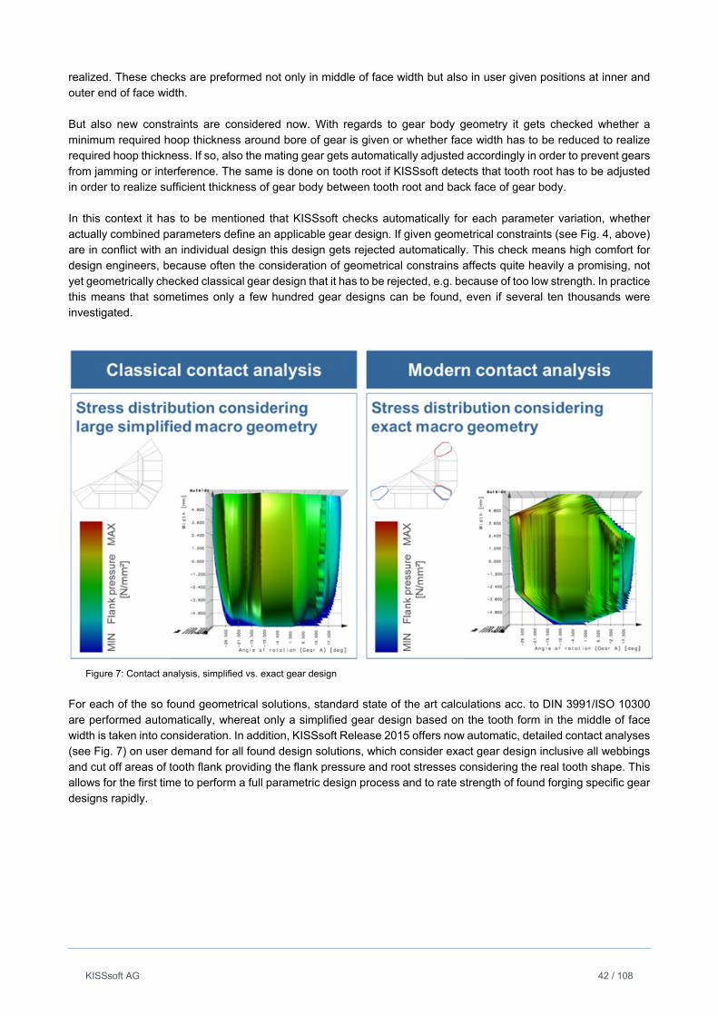
Figure 7: Contact analysis, simplified vs. exact gear design
For each of the so found geometrical solutions, standard state of the art calculations acc. to DIN 3991/ISO 10300 are performed automatically, whereat only a simplified gear design based on the tooth form in the middle of face width is taken into consideration. In addition, KISSsoft Release 2015 offers now automatic, detailed contact analyses (see Fig. 7) on user demand for all found design solutions, which consider exact gear design inclusive all webbings and cut off areas of tooth flank providing the flank pressure and root stresses considering the real tooth shape. This allows for the first time to perform a full parametric design process and to rate strength of found forging specific gear designs rapidly.
KISSsoft AG 43 / 108
Number of variants vs. runtime
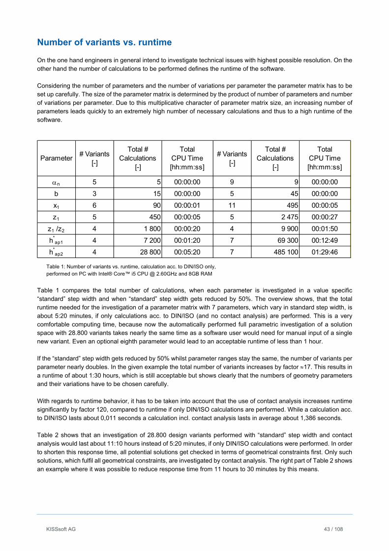
On the one hand engineers in general intend to investigate technical issues with highest possible resolution. On the other hand the number of calculations to be performed defines the runtime of the software. Considering the number of parameters and the number of variations per parameter the parameter matrix has to be set up carefully. The size of the parameter matrix is determined by the product of number of parameters and number of variations per parameter. Due to this multiplicative character of parameter matrix size, an increasing number of parameters leads quickly to an extremely high number of necessary calculations and thus to a high runtime of the software.
Table 1: Number of variants vs. runtime, calculation acc. to DIN/ISO only, performed on PC with Intel® Core™ i5 CPU @ 2.60GHz and 8GB RAM
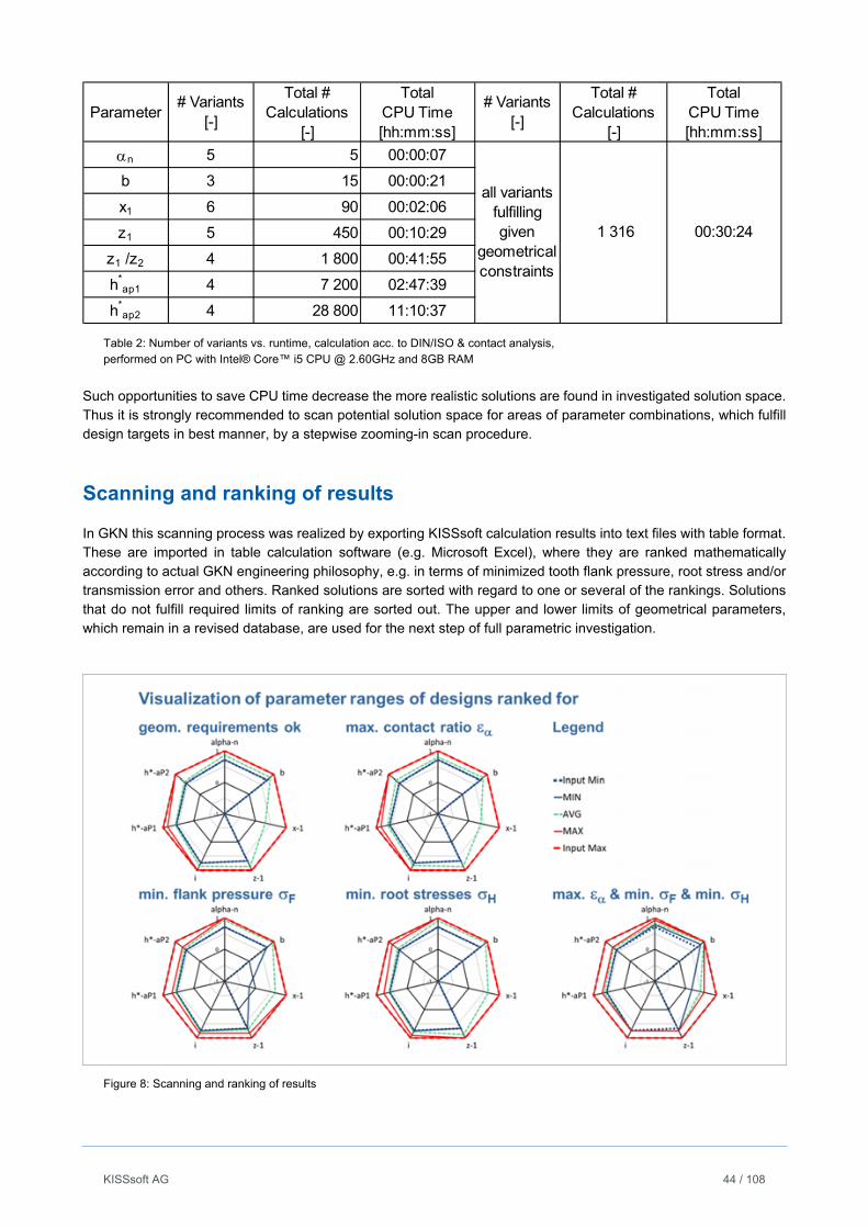
Table 1 compares the total number of calculations, when each parameter is investigated in a value specific “standard” step width and when “standard” step width gets reduced by 50%. The overview shows, that the total runtime needed for the investigation of a parameter matrix with 7 parameters, which vary in standard step width, is about 5:20 minutes, if only calculations acc. to DIN/ISO (and no contact analysis) are performed. This is a very comfortable computing time, because now the automatically performed full parametric investigation of a solution space with 28.800 variants takes nearly the same time as a software user would need for manual input of a single new variant. Even an optional eighth parameter would lead to an acceptable runtime of less than 1 hour. If the “standard” step width gets reduced by 50% whilst parameter ranges stay the same, the number of variants per parameter nearly doubles. In the given example the total number of variants increases by factor 17. This results in a runtime of about 1:30 hours, which is still acceptable but shows clearly that the numbers of geometry parameters and their variations have to be chosen carefully. With regards to runtime behavior, it has to be taken into account that the use of contact analysis increases runtime significantly by factor 120, compared to runtime if only DIN/ISO calculations are performed. While a calculation acc. to DIN/ISO lasts about 0,011 seconds a calculation incl. contact analysis lasts in average about 1,386 seconds. Table 2 shows that an investigation of 28.800 design variants performed with “standard” step width and contact analysis would last about 11:10 hours instead of 5:20 minutes, if only DIN/ISO calculations were performed. In order to shorten this response time, all potential solutions get checked in terms of geometrical constraints first. Only such solutions, which fulfil all geometrical constraints, are investigated by contact analysis. The right part of Table 2 shows an example where it was possible to reduce response time from 11 hours to 30 minutes by this means.
Parameter# Variants
[-]
Total # Calculations
[-]
TotalCPU Time[hh:mm:ss]
# Variants[-]
Total # Calculations
[-]
TotalCPU Time[hh:mm:ss]
n 5 5 00:00:00 9 9 00:00:00
b 3 15 00:00:00 5 45 00:00:00
x1 6 90 00:00:01 11 495 00:00:05
z1 5 450 00:00:05 5 2 475 00:00:27
z1 /z2 4 1 800 00:00:20 4 9 900 00:01:50
h*ap1 4 7 200 00:01:20 7 69 300 00:12:49
h*ap2 4 28 800 00:05:20 7 485 100 01:29:46
KISSsoft AG 44 / 108
Table 2: Number of variants vs. runtime, calculation acc. to DIN/ISO & contact analysis, performed on PC with Intel® Core™ i5 CPU @ 2.60GHz and 8GB RAM
Such opportunities to save CPU time decrease the more realistic solutions are found in investigated solution space. Thus it is strongly recommended to scan potential solution space for areas of parameter combinations, which fulfill design targets in best manner, by a stepwise zooming-in scan procedure.
Scanning and ranking of results
In GKN this scanning process was realized by exporting KISSsoft calculation results into text files with table format. These are imported in table calculation software (e.g. Microsoft Excel), where they are ranked mathematically according to actual GKN engineering philosophy, e.g. in terms of minimized tooth flank pressure, root stress and/or transmission error and others. Ranked solutions are sorted with regard to one or several of the rankings. Solutions that do not fulfill required limits of ranking are sorted out. The upper and lower limits of geometrical parameters, which remain in a revised database, are used for the next step of full parametric investigation.
Figure 8: Scanning and ranking of results
Parameter# Variants
[-]
Total # Calculations
[-]
TotalCPU Time[hh:mm:ss]
# Variants[-]
Total # Calculations
[-]
TotalCPU Time[hh:mm:ss]
n 5 5 00:00:07
b 3 15 00:00:21
x1 6 90 00:02:06
z1 5 450 00:10:29
z1 /z2 4 1 800 00:41:55
h*ap1 4 7 200 02:47:39
h*ap2 4 28 800 11:10:37
all variants fulfilling given
geometrical constraints
1 316 00:30:24
KISSsoft AG 45 / 108
Figure 8 shows an example for reduction of parameter space by consideration of single and combined rankings. In this case the upper left diagram shows that design parameters of design variants, which fulfill all geometrical requirements, are spread over the entire software user given parameter ranges. Only the range of addendum coefficient h*aP1 could not be used entirely. In the upper middle diagram similar information is given for parameter ranges of designs that fulfill all geometrical requirements and offer additionally maximum values for contact ratio . Here the graph of average parameter values indicates that these designs differ from the earlier shown. More impact on usable design parameter ranges can be detected for designs that fulfill all geometrical requirements and offer additionally minimum values for root stresses F or flank pressure H. Finally, the diagram for designs, which fulfill all geometrical requirements and offer additionally both maximum values of contact ratio as well as minimum values for root stresses F or flank pressure H, shows very narrow design parameter ranges. These ranges can be used for a next design parameter scan. To perform such scanning and ranking several times in sequence allows finding a design of high robustness related to its design targets and ensures that the finally chosen design is verifiable one of best possible solutions.
Summary and Outlook
GKN has successfully generated a new generic design process that allows developing forging specific bevel gear designs used in differentials according to defined design and performance criteria. This was made possible by KISSsoft AG by introducing customized software modules that allow adjusting gear design acc. to differential bevel gear specific requirements on geometry and by offering both processes, the strength calculation acc. to ISO as well as the fast contact analysis considering the real tooth shape of bevel gears with forging specific tooth design. The next step is to combine the wide design parameter variation of gear macro geometry with a wide design parameter variation of gear micro geometry. Therefore similar methods are in progress to define optimized micro geometries for given macro geometry. They are expected to be coming soon. These software tools will help to find a robust optimum in bevel gear macro and micro geometry with minimized packaging for GKN’s AWD and eDrive product stream applications - including special NVH performance characteristics required by AWD Booster™ disconnect drivetrains – to meet both performance and manufacturability constraints.
Literature
[1] ISO 10300-1:2014-04 (E), Calculation of load capacity of bevel gears - Part 1: Introduction and general influence factors, Berlin, Beuth Verlag GmbH
[2] ISO 10300-2:2014-04 (E), Calculation of load capacity of bevel gears - Part 2: Calculation of surface durability (pitting), Berlin, Beuth Verlag GmbH
[3] ISO 10300-3:2014-04 (E) Calculation of load capacity of bevel gears - Part 3: Calculation of tooth root strength, Berlin, Beuth Verlag GmbH
[4] KISSsoft, Machine Elements Calculation Software, www.KISSsoft.AG, 2015
[5] DIN 3991-1:1988-09 (D), Tragfähigkeitsberechnung von Kegelrädern ohne Achsversetzung; Einführung und allgemeine Einflußfaktoren, Berlin, Beuth Verlag GmbH
[6] DIN 3991-2:1988-09 (D), Tragfähigkeitsberechnung von Kegelrädern ohne Achsversetzung; Berechnung der Grübchentragfähigkeit, Berlin, Beuth Verlag GmbH
[7] DIN 3991-3:1988-09 (D), Tragfähigkeitsberechnung von Kegelrädern ohne Achsversetzung; Berechnung der Zahnfußtragfähigkeit, Berlin, Beuth Verlag GmbH
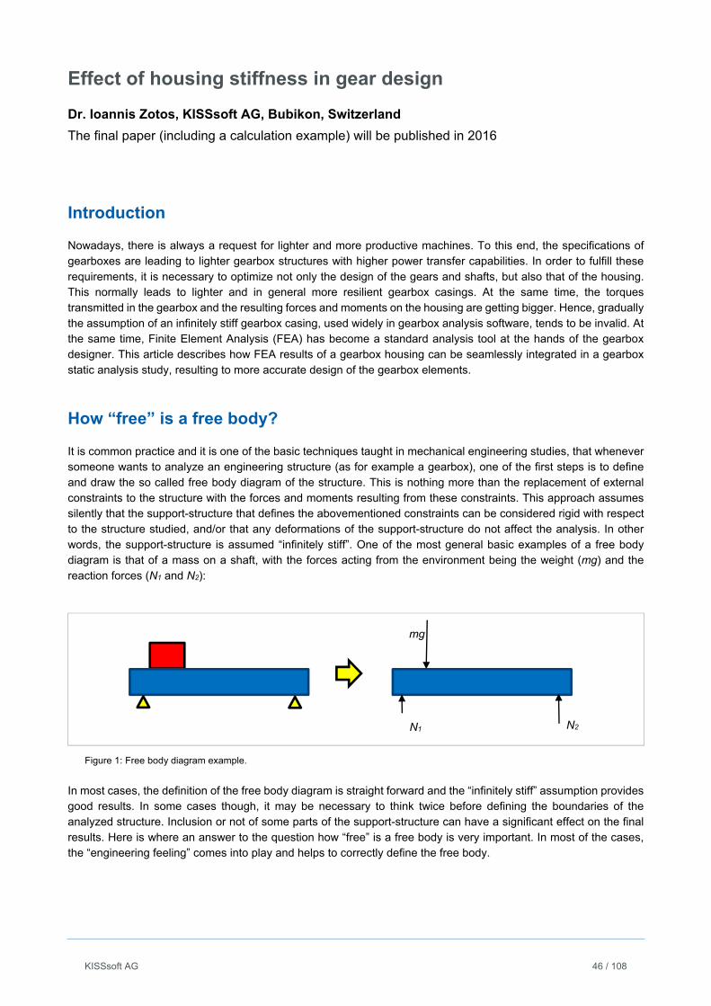
KISSsoft AG 46 / 108
Effect of housing stiffness in gear design
Dr. Ioannis Zotos, KISSsoft AG, Bubikon, Switzerland
The final paper (including a calculation example) will be published in 2016
Introduction
Nowadays, there is always a request for lighter and more productive machines. To this end, the specifications of gearboxes are leading to lighter gearbox structures with higher power transfer capabilities. In order to fulfill these requirements, it is necessary to optimize not only the design of the gears and shafts, but also that of the housing. This normally leads to lighter and in general more resilient gearbox casings. At the same time, the torques transmitted in the gearbox and the resulting forces and moments on the housing are getting bigger. Hence, gradually the assumption of an infinitely stiff gearbox casing, used widely in gearbox analysis software, tends to be invalid. At the same time, Finite Element Analysis (FEA) has become a standard analysis tool at the hands of the gearbox designer. This article describes how FEA results of a gearbox housing can be seamlessly integrated in a gearbox static analysis study, resulting to more accurate design of the gearbox elements.
How “free” is a free body?
It is common practice and it is one of the basic techniques taught in mechanical engineering studies, that whenever someone wants to analyze an engineering structure (as for example a gearbox), one of the first steps is to define and draw the so called free body diagram of the structure. This is nothing more than the replacement of external constraints to the structure with the forces and moments resulting from these constraints. This approach assumes silently that the support-structure that defines the abovementioned constraints can be considered rigid with respect to the structure studied, and/or that any deformations of the support-structure do not affect the analysis. In other words, the support-structure is assumed “infinitely stiff”. One of the most general basic examples of a free body diagram is that of a mass on a shaft, with the forces acting from the environment being the weight (mg) and the reaction forces (N1 and N2):
Figure 1: Free body diagram example.
In most cases, the definition of the free body diagram is straight forward and the “infinitely stiff” assumption provides good results. In some cases though, it may be necessary to think twice before defining the boundaries of the analyzed structure. Inclusion or not of some parts of the support-structure can have a significant effect on the final results. Here is where an answer to the question how “free” is a free body is very important. In most of the cases, the “engineering feeling” comes into play and helps to correctly define the free body.
N2
mg
N1
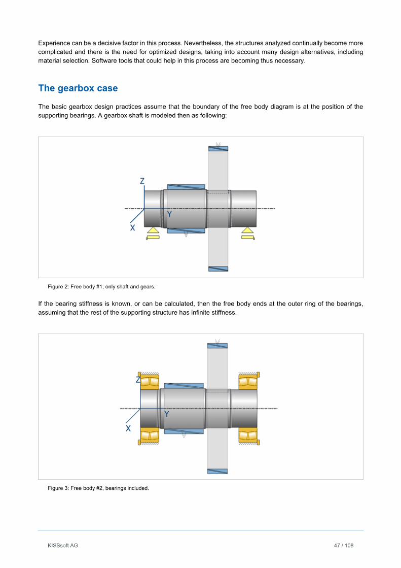
KISSsoft AG 47 / 108
Experience can be a decisive factor in this process. Nevertheless, the structures analyzed continually become more complicated and there is the need for optimized designs, taking into account many design alternatives, including material selection. Software tools that could help in this process are becoming thus necessary.
The gearbox case
The basic gearbox design practices assume that the boundary of the free body diagram is at the position of the supporting bearings. A gearbox shaft is modeled then as following:
Figure 2: Free body #1, only shaft and gears.
If the bearing stiffness is known, or can be calculated, then the free body ends at the outer ring of the bearings, assuming that the rest of the supporting structure has infinite stiffness.
Figure 3: Free body #2, bearings included.
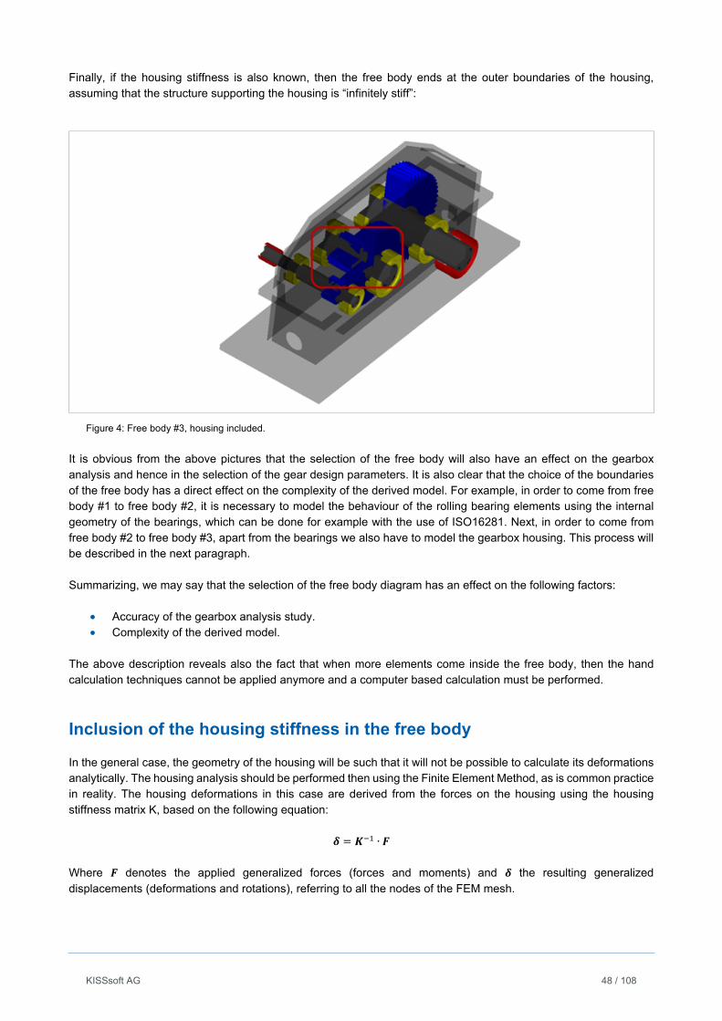
KISSsoft AG 48 / 108
Finally, if the housing stiffness is also known, then the free body ends at the outer boundaries of the housing, assuming that the structure supporting the housing is “infinitely stiff”:
Figure 4: Free body #3, housing included.
It is obvious from the above pictures that the selection of the free body will also have an effect on the gearbox analysis and hence in the selection of the gear design parameters. It is also clear that the choice of the boundaries of the free body has a direct effect on the complexity of the derived model. For example, in order to come from free body #1 to free body #2, it is necessary to model the behaviour of the rolling bearing elements using the internal geometry of the bearings, which can be done for example with the use of ISO16281. Next, in order to come from free body #2 to free body #3, apart from the bearings we also have to model the gearbox housing. This process will be described in the next paragraph. Summarizing, we may say that the selection of the free body diagram has an effect on the following factors:
Accuracy of the gearbox analysis study. Complexity of the derived model.
The above description reveals also the fact that when more elements come inside the free body, then the hand calculation techniques cannot be applied anymore and a computer based calculation must be performed.
Inclusion of the housing stiffness in the free body
In the general case, the geometry of the housing will be such that it will not be possible to calculate its deformations analytically. The housing analysis should be performed then using the Finite Element Method, as is common practice in reality. The housing deformations in this case are derived from the forces on the housing using the housing stiffness matrix K, based on the following equation:
∙ Where denotes the applied generalized forces (forces and moments) and the resulting generalized displacements (deformations and rotations), referring to all the nodes of the FEM mesh.
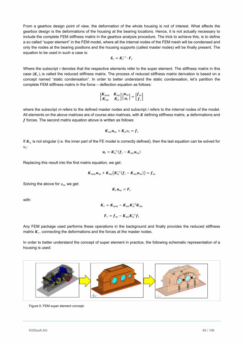
KISSsoft AG 49 / 108
From a gearbox design point of view, the deformation of the whole housing is not of interest. What affects the gearbox design is the deformations of the housing at the bearing locations. Hence, it is not actually necessary to include the complete FEM stiffness matrix in the gearbox analysis procedure. The trick to achieve this, is to define a so called “super element” in the FEM model, where all the internal nodes of the FEM mesh will be condensed and only the nodes at the bearing positions and the housing supports (called master nodes) will be finally present. The equation to be used in such a case is:
∙ Where the subscript r denotes that the respective elements refer to the super element. The stiffness matrix in this case ( ,is called the reduced stiffness matrix. The process of reduced stiffness matrix derivation is based on a concept named “static condensation”. In order to better understand the static condensation, let’s partition the complete FEM stiffness matrix in the force – deflection equation as follows:
where the subscript m refers to the defined master nodes and subscript i refers to the internal nodes of the model. All elements on the above matrices are of course also matrices, with defining stiffness matrix, deformations and
forces. The second matrix equation above is written as follows:
If is not singular (i.e. the inner part of the FE model is correctly defined), then the last equation can be solved for
:
Replacing this result into the first matrix equation, we get:
Solving the above for we get:
with:
Any FEM package used performs these operations in the background and finally provides the reduced stiffness matrix , connecting the deformations and the forces at the master nodes. In order to better understand the concept of super element in practice, the following schematic representation of a housing is used:
Figure 5: FEM super element concept.

KISSsoft AG 50 / 108
The left picture above shows the 3D model of the housing and other gearbox elements. In the middle picture, the complete FEM model of the housing with all the FEM nodes and elements included is shown. The positions of the bearings and the housing supports are shown with red shapes (master nodes). Finally, in the right picture all the other FEM nodes of the housing are condensed and only the master nodes in the red shapes are kept. Hence, the housing is represented by the fictitious springs that connect the master nodes. In reality there are fictitious springs connecting the master nodes in pairs in every possible combination and for all degrees of freedom, but it would be impossible to draw so many springs in the above picture. It should be mentioned here that any initial offsets of the bearings positions due to static external forces on the housing, thermal expansion, bearings preloads, etc. must be applied directly on the bearings. Any extra movements of the bearings during the gearbox operation due to the housing resilience is then added to the above (principle of superposition – assumption of linear housing). Using the derived reduced stiffness matrix, it is possible to calculate the generalized deformations at the master nodes due to the generalized forces applied to them. Hence the positions of the supporting bearings due to the deformation of the housing can be derived. This will also include the cross-coupling of the gearbox shafts through the housing structure, leading to a more realistic analysis of the gearbox. Since the bearings will be moved to a different position than the initially assumed, it will be necessary to recalculate the forces applied on the housing due to these new positions, by running a static calculation on the shafts. The whole process must be repeated until convergence is achieved, i.e. no more change in housing forces or bearing positions is calculated. A schematic representation of this convergence loop can be seen next:
Figure 6: Convergence loop diagram.
Based on the final converged positions of the bearings, the contact pattern on the mating gears can be calculated. In general, this will be different to the one derived assumed the bearing positions to be fixed (infinitely stiff housing). This fact should be taken into account in defining the gear modifications, in order to achieve optimum meshing contact. The final positions of the bearings could also have an effect on the life calculation of them. In brief, the whole analysis of the structure will lead to completely different results, since the definition of the problem will change.

KISSsoft AG 51 / 108
Conclusions
The gearbox housing design should be an integral part of the analysis and design of the shafts, bearings and gears of the gearbox. Any design change to one of them, should be communicated and used in the analysis of the rest. All of these parts should be considered simultaneously in an optimization study of a gearbox. Hence the engineers involved in gearbox analysis and design should not only be informed about, but also understand the importance of the housing stiffness for their studies. Since the whole process is quite involved, correct computer tools should be used as an aid in this design task.
KISSsoft AG 52 / 108
Gear strength when operating a gearbox at resonance and considering transient events using a mill drive as example
Hanspeter Dinner, Managing Director, EES KISSsoft GmbH, Switzerland
Dipl.-Ing. ETH Marco Perucchi, DELTA JS AG, Switzerland
Paper presented at the “Dresdner Maschinenelemente Kolloquium 2015”
1. Summary
In gearboxes subjected to high and fluctuating torque loads, the gear design with respect to gear strength and with respect to gear modifications is challenging. Suitable engineering tools for the simulation of vibration or transient loads as well as tools for the gear geometry and strength calculation are available and need to be combined in an effective manner. For the dynamic analysis of multi stage gearboxes, considering the gearbox as a single spring-mass element is not sufficiently accurate. Only a model consisting of several elements, each representing a gear or a shaft allows the calculation of the forces acting in each gear mesh separately. This in turn is necessary to perform a strength verification for each stage based on local loads, expressed as a stage specific load duration distribution LDD. For this, dynamic tooth forces are superimposed to static tooth loads. From this, for each gear mesh, an individual loads spectrum results which then allows for an individual damage accumulation calculation. The investigation documented here is limited to torsional vibrations. Using a sugar mill gearbox as example, we show that he use of a global “application factor” may be conservative and may lead to an unfavourable design. For this, the CAE tools “MADYN 2000” (rotor dynamics) and KISSsoft (static analysis) are combined allowing a realistic strength assessment with limited effort. In the gearbox investigated, it was shown that for all gear stages, except the bevel gear stage, the original design was conservative. Damages calculated using load spectra based on dynamic simulation yielded lower values compared to the calculation using nominal loads multiplied with an application factor. For the bevel gear stage it could also be shown that the modifications used needed to be changed to avoid edge contact under certain operating conditions.
2. Introduction and application
Sugar cane is shredded between two rollers equipped with knives before it is pressed to extract the juice. The shredding process increases the efficiency of the sugar extraction to 95%-97%. The rollers are driven by a gearbox with two output shafts. The rollers and the gearbox output shafts are connected by connecting shafts with square hubs. The gearbox is driven by an electric motor or by a steam turbine, the later using the heat generated in various subsequent processes. The number of knives on the rollers may vary, see Figure 3. Whenever a new row of knives is engaged, the drive train is being excited. The frequency of excitation is equal to the rotational speed of the rollers multiplied by twice the number of knives on the roller (the knives are meshing with each other like a gear pair).
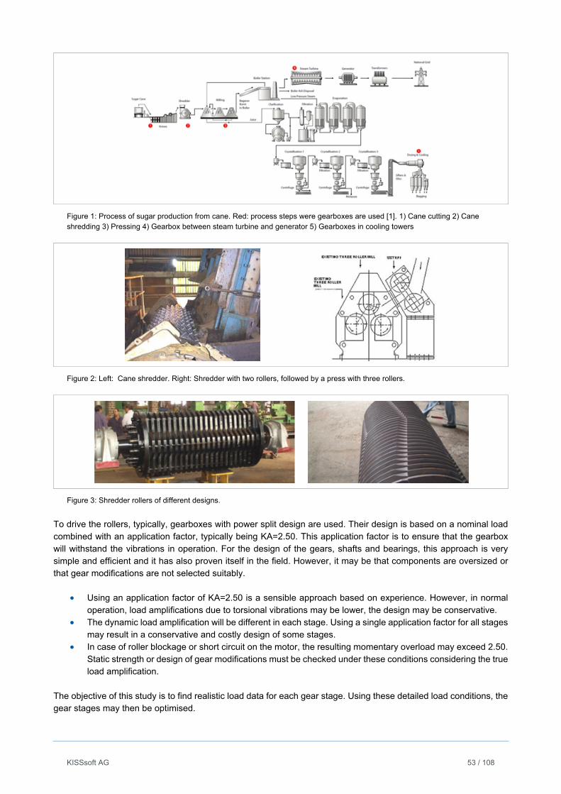
KISSsoft AG 53 / 108
Figure 1: Process of sugar production from cane. Red: process steps were gearboxes are used [1]. 1) Cane cutting 2) Cane shredding 3) Pressing 4) Gearbox between steam turbine and generator 5) Gearboxes in cooling towers
Figure 2: Left: Cane shredder. Right: Shredder with two rollers, followed by a press with three rollers.
Figure 3: Shredder rollers of different designs.
To drive the rollers, typically, gearboxes with power split design are used. Their design is based on a nominal load combined with an application factor, typically being KA=2.50. This application factor is to ensure that the gearbox will withstand the vibrations in operation. For the design of the gears, shafts and bearings, this approach is very simple and efficient and it has also proven itself in the field. However, it may be that components are oversized or that gear modifications are not selected suitably.
Using an application factor of KA=2.50 is a sensible approach based on experience. However, in normal operation, load amplifications due to torsional vibrations may be lower, the design may be conservative.
The dynamic load amplification will be different in each stage. Using a single application factor for all stages may result in a conservative and costly design of some stages.
In case of roller blockage or short circuit on the motor, the resulting momentary overload may exceed 2.50. Static strength or design of gear modifications must be checked under these conditions considering the true load amplification.
The objective of this study is to find realistic load data for each gear stage. Using these detailed load conditions, the gear stages may then be optimised.
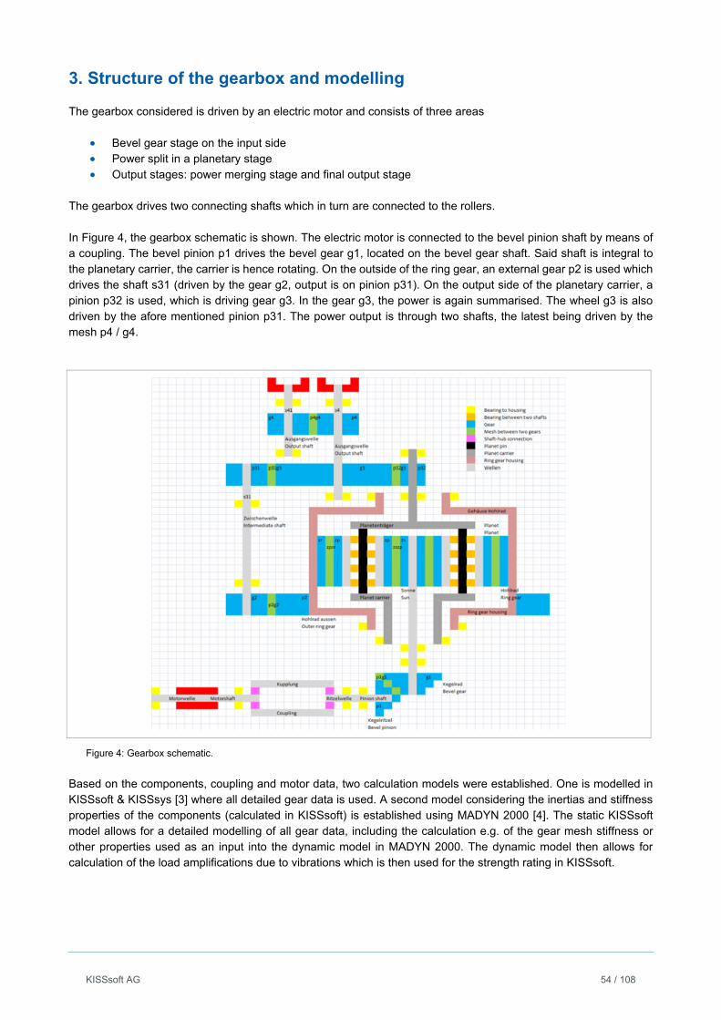
KISSsoft AG 54 / 108
3. Structure of the gearbox and modelling
The gearbox considered is driven by an electric motor and consists of three areas
Bevel gear stage on the input side Power split in a planetary stage Output stages: power merging stage and final output stage
The gearbox drives two connecting shafts which in turn are connected to the rollers. In Figure 4, the gearbox schematic is shown. The electric motor is connected to the bevel pinion shaft by means of a coupling. The bevel pinion p1 drives the bevel gear g1, located on the bevel gear shaft. Said shaft is integral to the planetary carrier, the carrier is hence rotating. On the outside of the ring gear, an external gear p2 is used which drives the shaft s31 (driven by the gear g2, output is on pinion p31). On the output side of the planetary carrier, a pinion p32 is used, which is driving gear g3. In the gear g3, the power is again summarised. The wheel g3 is also driven by the afore mentioned pinion p31. The power output is through two shafts, the latest being driven by the mesh p4 / g4.
Figure 4: Gearbox schematic.
Based on the components, coupling and motor data, two calculation models were established. One is modelled in KISSsoft & KISSsys [3] where all detailed gear data is used. A second model considering the inertias and stiffness properties of the components (calculated in KISSsoft) is established using MADYN 2000 [4]. The static KISSsoft model allows for a detailed modelling of all gear data, including the calculation e.g. of the gear mesh stiffness or other properties used as an input into the dynamic model in MADYN 2000. The dynamic model then allows for calculation of the load amplifications due to vibrations which is then used for the strength rating in KISSsoft.
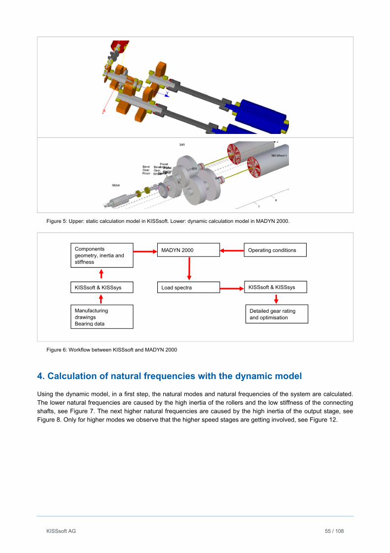
KISSsoft AG 55 / 108
Figure 5: Upper: static calculation model in KISSsoft. Lower: dynamic calculation model in MADYN 2000.
Figure 6: Workflow between KISSsoft and MADYN 2000
4. Calculation of natural frequencies with the dynamic model
Using the dynamic model, in a first step, the natural modes and natural frequencies of the system are calculated. The lower natural frequencies are caused by the high inertia of the rollers and the low stiffness of the connecting shafts, see Figure 7. The next higher natural frequencies are caused by the high inertia of the output stage, see Figure 8. Only for higher modes we observe that the higher speed stages are getting involved, see Figure 12.
Manufacturing drawings Bearing data
KISSsoft & KISSsys
Components geometry, inertia and stiffness
MADYN 2000
Detailed gear rating and optimisation
Operating conditions
Load spectra KISSsoft & KISSsys
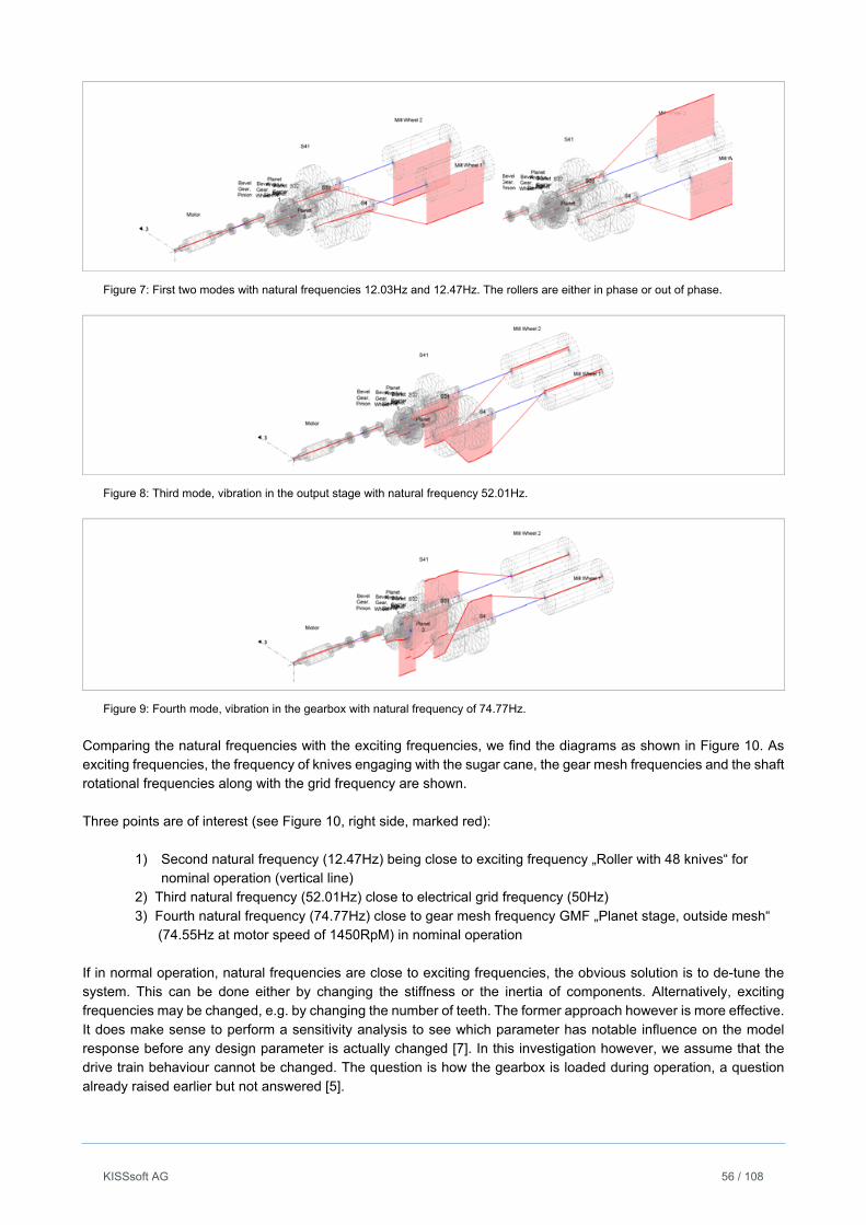
KISSsoft AG 56 / 108
Figure 7: First two modes with natural frequencies 12.03Hz and 12.47Hz. The rollers are either in phase or out of phase.
Figure 8: Third mode, vibration in the output stage with natural frequency 52.01Hz.
Figure 9: Fourth mode, vibration in the gearbox with natural frequency of 74.77Hz.
Comparing the natural frequencies with the exciting frequencies, we find the diagrams as shown in Figure 10. As exciting frequencies, the frequency of knives engaging with the sugar cane, the gear mesh frequencies and the shaft rotational frequencies along with the grid frequency are shown. Three points are of interest (see Figure 10, right side, marked red):
1) Second natural frequency (12.47Hz) being close to exciting frequency „Roller with 48 knives“ for
nominal operation (vertical line) 2) Third natural frequency (52.01Hz) close to electrical grid frequency (50Hz) 3) Fourth natural frequency (74.77Hz) close to gear mesh frequency GMF „Planet stage, outside mesh“ (74.55Hz at motor speed of 1450RpM) in nominal operation
If in normal operation, natural frequencies are close to exciting frequencies, the obvious solution is to de-tune the system. This can be done either by changing the stiffness or the inertia of components. Alternatively, exciting frequencies may be changed, e.g. by changing the number of teeth. The former approach however is more effective. It does make sense to perform a sensitivity analysis to see which parameter has notable influence on the model response before any design parameter is actually changed [7]. In this investigation however, we assume that the drive train behaviour cannot be changed. The question is how the gearbox is loaded during operation, a question already raised earlier but not answered [5].
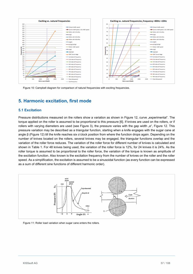
KISSsoft AG 57 / 108
Figure 10: Campbell diagram for comparison of natural frequencies with exciting frequencies.
5. Harmonic excitation, first mode
5.1 Excitation
Pressure distributions measured on the rollers show a variation as shown in Figure 12, curve „experimental“. The torque applied on the roller is assumed to be proportional to this pressure [6]. If knives are used on the rollers, or if rollers with varying diameters are used (see Figure 3), the pressure varies with the gap width „e“, Figure 12. This pressure variation may be described as a triangular function, starting when a knife engages with the sugar cane at angle β (Figure 12) till the knife reaches six o’clock position from where the function drops again. Depending on the number of knives located on the rollers, several knives may be engaged, the triangular functions overlap and the variation of the roller force reduces. The variation of the roller force for different number of knives is calculated and shown in Table 1. For 48 knives being used, the variation of the roller force is 12%, for 24 knives it is 24%. As the roller torque is assumed to be proportional to the roller force, the variation of the torque is known as amplitude of the excitation function. Also known is the excitation frequency from the number of knives on the roller and the roller speed. As a simplification, the excitation is assumed to be a sinusoidal function (as every function can be expressed as a sum of different sine functions of different harmonic order).
Figure 11: Roller load variation when sugar cane enters the rollers.
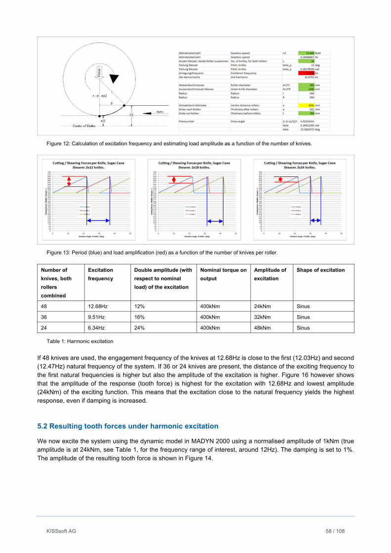
KISSsoft AG 58 / 108
Figure 12: Calculation of excitation frequency and estimating load amplitude as a function of the number of knives.
Figure 13: Period (blue) and load amplification (red) as a function of the number of knives per roller.
Number of
knives, both
rollers
combined
Excitation
frequency
Double amplitude (with
respect to nominal
load) of the excitation
Nominal torque on
output
Amplitude of
excitation
Shape of excitation
48 12.68Hz 12% 400kNm 24kNm Sinus
36 9.51Hz 16% 400kNm 32kNm Sinus
24 6.34Hz 24% 400kNm 48kNm Sinus
Table 1: Harmonic excitation
If 48 knives are used, the engagement frequency of the knives at 12.68Hz is close to the first (12.03Hz) and second (12.47Hz) natural frequency of the system. If 36 or 24 knives are present, the distance of the exciting frequency to the first natural frequencies is higher but also the amplitude of the excitation is higher. Figure 16 however shows that the amplitude of the response (tooth force) is highest for the excitation with 12.68Hz and lowest amplitude (24kNm) of the exciting function. This means that the excitation close to the natural frequency yields the highest response, even if damping is increased.
5.2 Resulting tooth forces under harmonic excitation
We now excite the system using the dynamic model in MADYN 2000 using a normalised amplitude of 1kNm (true amplitude is at 24kNm, see Table 1, for the frequency range of interest, around 12Hz). The damping is set to 1%. The amplitude of the resulting tooth force is shown in Figure 14.
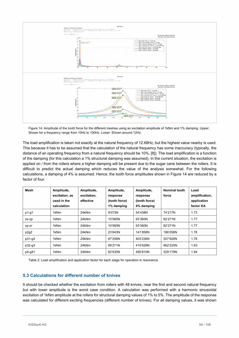
KISSsoft AG 59 / 108
Figure 14: Amplitude of the tooth force for the different meshes using an excitation amplitude of 1kNm and 1% damping. Upper: Shown for a frequency range from 10Hz to 100Hz. Lower: Shown around 12Hz.
The load amplification is taken not exactly at the natural frequency of 12.68Hz, but the highest value nearby is used. This because it has to be assumed that the calculation of the natural frequency has some inaccuracy (typically, the distance of an operating frequency from a natural frequency should be 10%, [8]). The load amplification is a function of the damping (for this calculation a 1% structural damping was assumed). In the current situation, the excitation is applied on / from the rollers where a higher damping will be present due to the sugar cane between the rollers. It is difficult to predict the actual damping which reduces the value of the analysis somewhat. For the following calculations, a damping of 4% is assumed. Hence, the tooth force amplitudes shown in Figure 14 are reduced by a factor of four.
Mesh Amplitude,
excitation, as
used in the
calculation
Amplitude,
excitation,
effective
Amplitude,
response
(tooth force)
1% damping
Amplitude,
response
(tooth force)
4% damping
Nominal tooth
force
Load
amplification,
application
factor KA
p1-g1 1kNm 24kNm 9‘073N 54‘438N 74‘217N 1.73
zs-zp 1kNm 24kNm 10‘560N 63‘360N 82‘271N 1.77
zp-zr 1kNm 24kNm 10‘560N 63‘360N 82‘271N 1.77
p2g2 1kNm 24kNm 23‘643N 141‘858N 186‘058N 1.76
p31-g3 1kNm 24kNm 67‘206N 403‘236N 527‘626N 1.76
p32-g3 1kNm 24kNm 69‘271N 415‘626N 662‘225N 1.63
p4-g41 1kNm 24kNm 82‘635N 495‘810N 529‘179N 1.94
Table 2: Load amplification and application factor for each stage for operation in resonance.
5.3 Calculations for different number of knives
It should be checked whether the excitation from rollers with 48 knives, near the first and second natural frequency but with lower amplitude is the worst case condition. A calculation was performed with a harmonic sinusoidal excitation of 1kNm amplitude at the rollers for structural damping values of 1% to 5%. The amplitude of the response was calculated for different exciting frequencies (different number of knives). For all damping values, it was shown
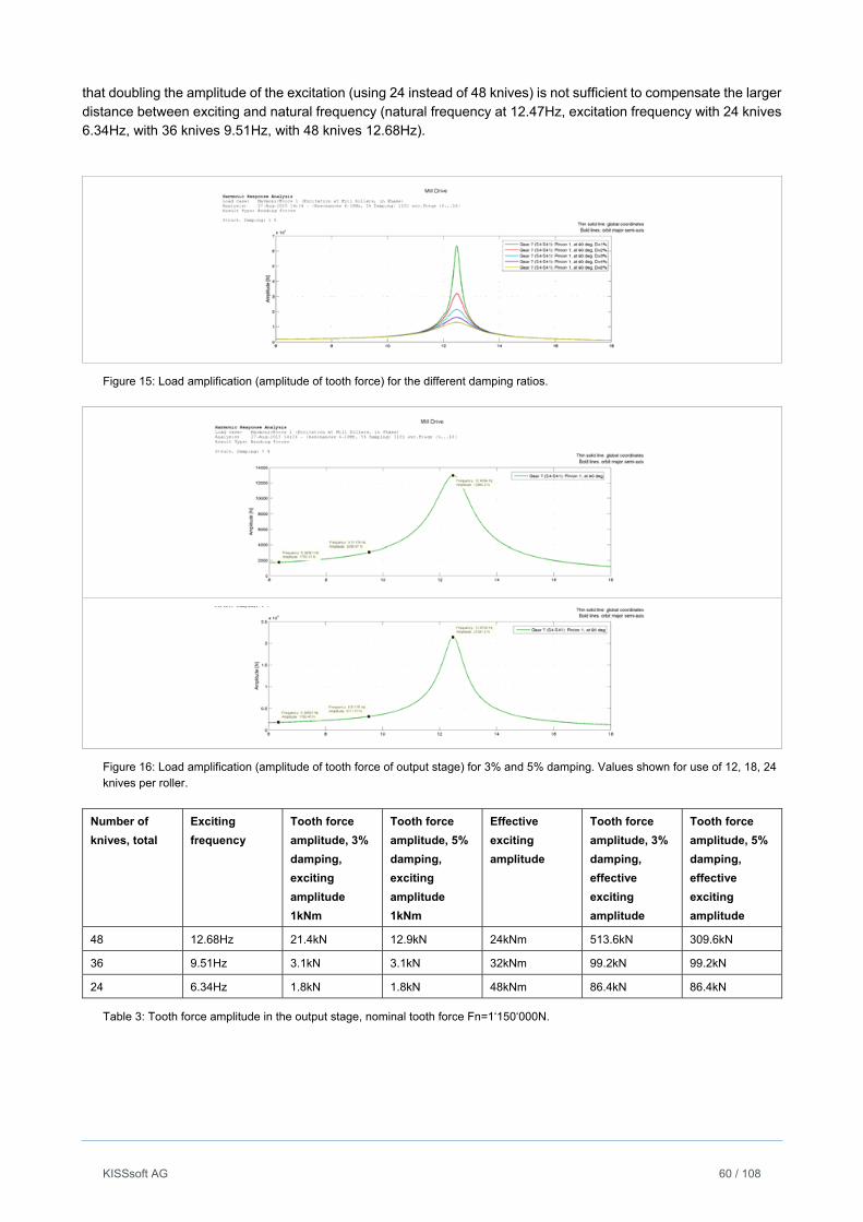
KISSsoft AG 60 / 108
that doubling the amplitude of the excitation (using 24 instead of 48 knives) is not sufficient to compensate the larger distance between exciting and natural frequency (natural frequency at 12.47Hz, excitation frequency with 24 knives 6.34Hz, with 36 knives 9.51Hz, with 48 knives 12.68Hz).
Figure 15: Load amplification (amplitude of tooth force) for the different damping ratios.
Figure 16: Load amplification (amplitude of tooth force of output stage) for 3% and 5% damping. Values shown for use of 12, 18, 24 knives per roller.
Number of
knives, total
Exciting
frequency
Tooth force
amplitude, 3%
damping,
exciting
amplitude
1kNm
Tooth force
amplitude, 5%
damping,
exciting
amplitude
1kNm
Effective
exciting
amplitude
Tooth force
amplitude, 3%
damping,
effective
exciting
amplitude
Tooth force
amplitude, 5%
damping,
effective
exciting
amplitude
48 12.68Hz 21.4kN 12.9kN 24kNm 513.6kN 309.6kN
36 9.51Hz 3.1kN 3.1kN 32kNm 99.2kN 99.2kN
24 6.34Hz 1.8kN 1.8kN 48kNm 86.4kN 86.4kN
Table 3: Tooth force amplitude in the output stage, nominal tooth force Fn=1‘150‘000N.
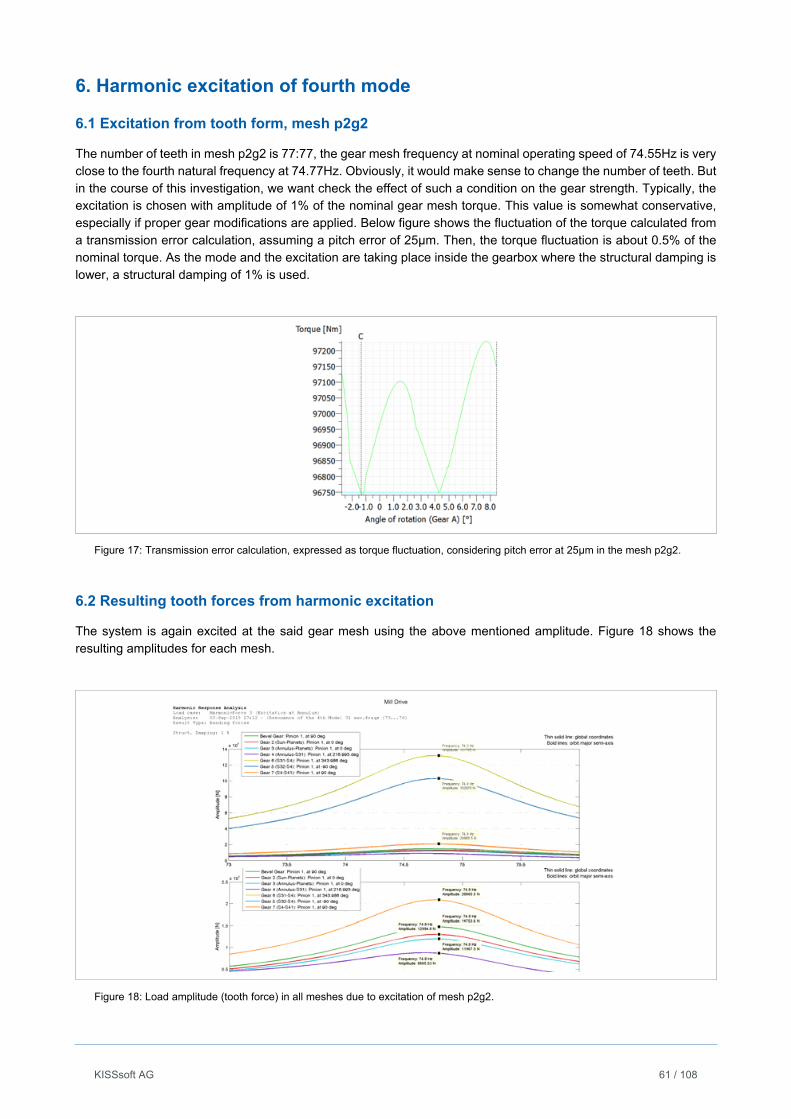
KISSsoft AG 61 / 108
6. Harmonic excitation of fourth mode
6.1 Excitation from tooth form, mesh p2g2
The number of teeth in mesh p2g2 is 77:77, the gear mesh frequency at nominal operating speed of 74.55Hz is very close to the fourth natural frequency at 74.77Hz. Obviously, it would make sense to change the number of teeth. But in the course of this investigation, we want check the effect of such a condition on the gear strength. Typically, the excitation is chosen with amplitude of 1% of the nominal gear mesh torque. This value is somewhat conservative, especially if proper gear modifications are applied. Below figure shows the fluctuation of the torque calculated from a transmission error calculation, assuming a pitch error of 25μm. Then, the torque fluctuation is about 0.5% of the nominal torque. As the mode and the excitation are taking place inside the gearbox where the structural damping is lower, a structural damping of 1% is used.
Figure 17: Transmission error calculation, expressed as torque fluctuation, considering pitch error at 25μm in the mesh p2g2.
6.2 Resulting tooth forces from harmonic excitation
The system is again excited at the said gear mesh using the above mentioned amplitude. Figure 18 shows the resulting amplitudes for each mesh.
Figure 18: Load amplitude (tooth force) in all meshes due to excitation of mesh p2g2.
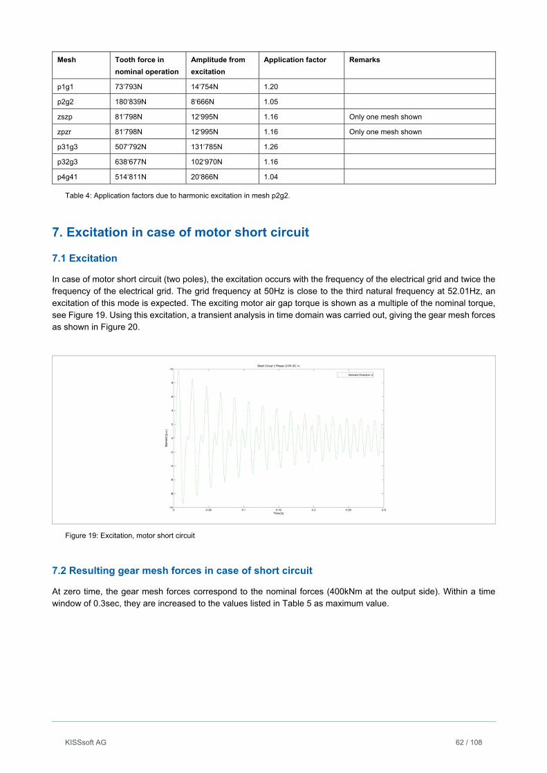
KISSsoft AG 62 / 108
Mesh Tooth force in
nominal operation
Amplitude from
excitation
Application factor Remarks
p1g1 73‘793N 14‘754N 1.20
p2g2 180‘839N 8‘666N 1.05
zszp 81‘798N 12‘995N 1.16 Only one mesh shown
zpzr 81‘798N 12‘995N 1.16 Only one mesh shown
p31g3 507‘792N 131‘785N 1.26
p32g3 638‘677N 102‘970N 1.16
p4g41 514‘811N 20‘866N 1.04
Table 4: Application factors due to harmonic excitation in mesh p2g2.
7. Excitation in case of motor short circuit
7.1 Excitation
In case of motor short circuit (two poles), the excitation occurs with the frequency of the electrical grid and twice the frequency of the electrical grid. The grid frequency at 50Hz is close to the third natural frequency at 52.01Hz, an excitation of this mode is expected. The exciting motor air gap torque is shown as a multiple of the nominal torque, see Figure 19. Using this excitation, a transient analysis in time domain was carried out, giving the gear mesh forces as shown in Figure 20.
Figure 19: Excitation, motor short circuit
7.2 Resulting gear mesh forces in case of short circuit
At zero time, the gear mesh forces correspond to the nominal forces (400kNm at the output side). Within a time window of 0.3sec, they are increased to the values listed in Table 5 as maximum value.
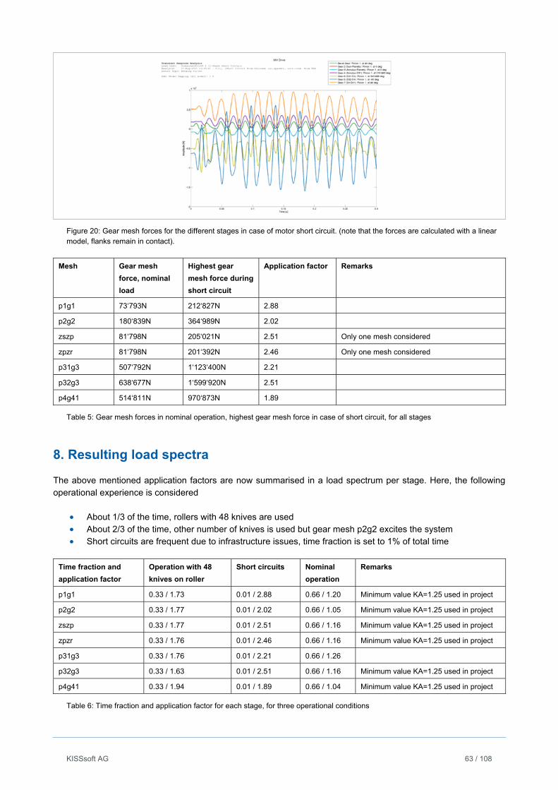
KISSsoft AG 63 / 108
Figure 20: Gear mesh forces for the different stages in case of motor short circuit. (note that the forces are calculated with a linear model, flanks remain in contact).
Mesh Gear mesh
force, nominal
load
Highest gear
mesh force during
short circuit
Application factor Remarks
p1g1 73‘793N 212‘827N 2.88
p2g2 180‘839N 364‘989N 2.02
zszp 81‘798N 205‘021N 2.51 Only one mesh considered
zpzr 81‘798N 201‘392N 2.46 Only one mesh considered
p31g3 507‘792N 1‘123‘400N 2.21
p32g3 638‘677N 1‘599‘920N 2.51
p4g41 514‘811N 970‘873N 1.89
Table 5: Gear mesh forces in nominal operation, highest gear mesh force in case of short circuit, for all stages
8. Resulting load spectra
The above mentioned application factors are now summarised in a load spectrum per stage. Here, the following operational experience is considered
About 1/3 of the time, rollers with 48 knives are used About 2/3 of the time, other number of knives is used but gear mesh p2g2 excites the system Short circuits are frequent due to infrastructure issues, time fraction is set to 1% of total time
Time fraction and
application factor
Operation with 48
knives on roller
Short circuits
Nominal
operation
Remarks
p1g1 0.33 / 1.73 0.01 / 2.88 0.66 / 1.20 Minimum value KA=1.25 used in project
p2g2 0.33 / 1.77 0.01 / 2.02 0.66 / 1.05 Minimum value KA=1.25 used in project
zszp 0.33 / 1.77 0.01 / 2.51 0.66 / 1.16 Minimum value KA=1.25 used in project
zpzr 0.33 / 1.76 0.01 / 2.46 0.66 / 1.16 Minimum value KA=1.25 used in project
p31g3 0.33 / 1.76 0.01 / 2.21 0.66 / 1.26
p32g3 0.33 / 1.63 0.01 / 2.51 0.66 / 1.16 Minimum value KA=1.25 used in project
p4g41 0.33 / 1.94 0.01 / 1.89 0.66 / 1.04 Minimum value KA=1.25 used in project
Table 6: Time fraction and application factor for each stage, for three operational conditions
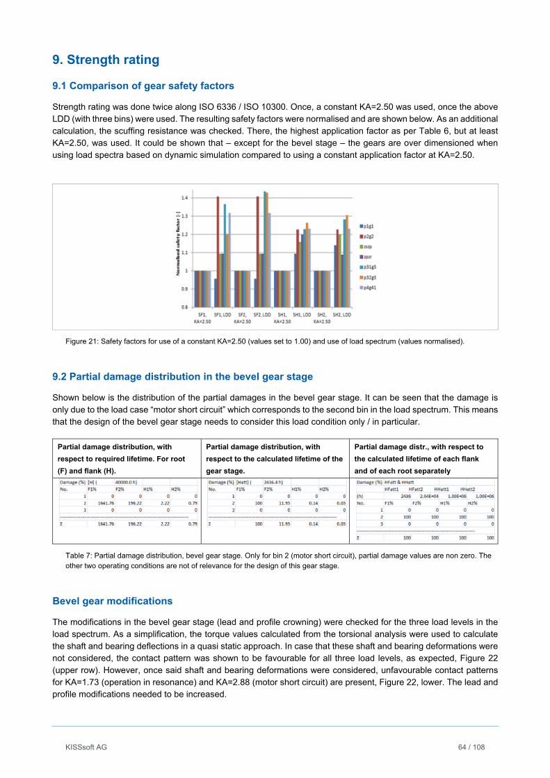
KISSsoft AG 64 / 108
9. Strength rating
9.1 Comparison of gear safety factors
Strength rating was done twice along ISO 6336 / ISO 10300. Once, a constant KA=2.50 was used, once the above LDD (with three bins) were used. The resulting safety factors were normalised and are shown below. As an additional calculation, the scuffing resistance was checked. There, the highest application factor as per Table 6, but at least KA=2.50, was used. It could be shown that – except for the bevel stage – the gears are over dimensioned when using load spectra based on dynamic simulation compared to using a constant application factor at KA=2.50.
Figure 21: Safety factors for use of a constant KA=2.50 (values set to 1.00) and use of load spectrum (values normalised).
9.2 Partial damage distribution in the bevel gear stage
Shown below is the distribution of the partial damages in the bevel gear stage. It can be seen that the damage is only due to the load case “motor short circuit” which corresponds to the second bin in the load spectrum. This means that the design of the bevel gear stage needs to consider this load condition only / in particular.
Partial damage distribution, with
respect to required lifetime. For root
(F) and flank (H).
Partial damage distribution, with
respect to the calculated lifetime of the
gear stage.
Partial damage distr., with respect to
the calculated lifetime of each flank
and of each root separately
Table 7: Partial damage distribution, bevel gear stage. Only for bin 2 (motor short circuit), partial damage values are non zero. The other two operating conditions are not of relevance for the design of this gear stage.
Bevel gear modifications
The modifications in the bevel gear stage (lead and profile crowning) were checked for the three load levels in the load spectrum. As a simplification, the torque values calculated from the torsional analysis were used to calculate the shaft and bearing deflections in a quasi static approach. In case that these shaft and bearing deformations were not considered, the contact pattern was shown to be favourable for all three load levels, as expected, Figure 22 (upper row). However, once said shaft and bearing deformations were considered, unfavourable contact patterns for KA=1.73 (operation in resonance) and KA=2.88 (motor short circuit) are present, Figure 22, lower. The lead and profile modifications needed to be increased.
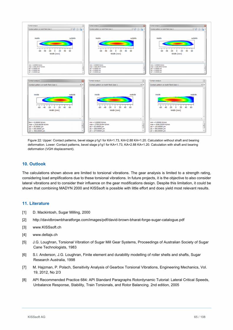
KISSsoft AG 65 / 108
Figure 22: Upper: Contact patterns, bevel stage p1g1 for KA=1.73, KA=2.88 KA=1.20. Calculation without shaft and bearing deformation. Lower: Contact patterns, bevel stage p1g1 for KA=1.73, KA=2.88 KA=1.20. Calculation with shaft and bearing deformation (VGH displacement).
10. Outlook
The calculations shown above are limited to torsional vibrations. The gear analysis is limited to a strength rating, considering load amplifications due to these torsional vibrations. In future projects, it is the objective to also consider lateral vibrations and to consider their influence on the gear modifications design. Despite this limitation, it could be shown that combining MADYN 2000 and KISSsoft is possible with little effort and does yield most relevant results.
11. Literature
[1] D. Mackintosh, Sugar Milling, 2000
[2] http://davidbrownbharatforge.com/images/pdf/david-brown-bharat-forge-sugar-catalogue.pdf
[3] www.KISSsoft.ch
[4] www.deltajs.ch
[5] J.G. Loughran, Torsional Vibration of Sugar Mill Gear Systems, Proceedings of Australian Society of Sugar Cane Technologists, 1983
[6] S.I. Anderson, J.G. Loughran, Finite element and durability modelling of roller shells and shafts, Sugar Research Australia, 1998
[7] M. Hajzman, P. Polach, Sensitivity Analysis of Gearbox Torsional Vibrations, Engineering Mechanics, Vol. 19, 2012, No 2/3
[8] API Recommended Practice 684: API Standard Paragraphs Rotordynamic Tutorial: Lateral Critical Speeds, Unbalance Response, Stability, Train Torsionals, and Rotor Balancing. 2nd edition, 2005

KISSsoft AG 66 / 108
Optimising a transmission for use with higher hp engine
Hanspeter Dinner, Managing Director, EES KISSsoft GmbH, Switzerland
Tractor Case Study 2015
1. Optimising a transmission for use with higher hp engine
Figure 1.1-1: TAFE is second largest tractor manufacturer by volume in India.
1.1 Objective of the project
Fitting a stronger motor to a tractor raises the question of torque capability of the transmission and how it can be optimised in a given design space to cope with the increased torque. Furthermore, vibration levels must be lowered or maintained and aspects of manufacturing like tool commonisation are to be considered. The transmission shown below is an existing design originally used with a 45hp motor. Key features of the transmission are: Configuration Transmission: Forward / reverse, low / high range, four speeds Axle: Bevel gear set and planetary final drive Power rating Using clubbed load spectrum covering all ten speeds Technology Modified, shaved high addendum helical gears. Gleason type ground spiral bevel gear. Spur gear planetary set in axle.
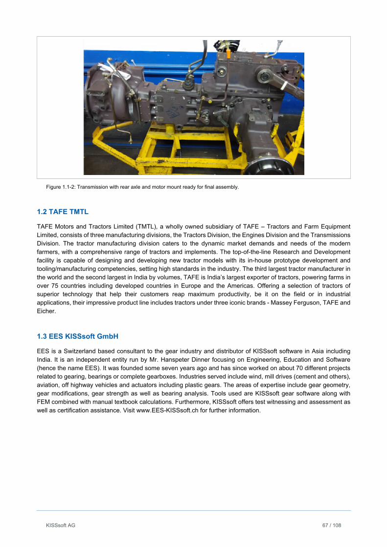
KISSsoft AG 67 / 108
Figure 1.1-2: Transmission with rear axle and motor mount ready for final assembly.
1.2 TAFE TMTL
TAFE Motors and Tractors Limited (TMTL), a wholly owned subsidiary of TAFE – Tractors and Farm Equipment Limited, consists of three manufacturing divisions, the Tractors Division, the Engines Division and the Transmissions Division. The tractor manufacturing division caters to the dynamic market demands and needs of the modern farmers, with a comprehensive range of tractors and implements. The top-of-the-line Research and Development facility is capable of designing and developing new tractor models with its in-house prototype development and tooling/manufacturing competencies, setting high standards in the industry. The third largest tractor manufacturer in the world and the second largest in India by volumes, TAFE is India’s largest exporter of tractors, powering farms in over 75 countries including developed countries in Europe and the Americas. Offering a selection of tractors of superior technology that help their customers reap maximum productivity, be it on the field or in industrial applications, their impressive product line includes tractors under three iconic brands - Massey Ferguson, TAFE and Eicher.
1.3 EES KISSsoft GmbH
EES is a Switzerland based consultant to the gear industry and distributor of KISSsoft software in Asia including India. It is an independent entity run by Mr. Hanspeter Dinner focusing on Engineering, Education and Software (hence the name EES). It was founded some seven years ago and has since worked on about 70 different projects related to gearing, bearings or complete gearboxes. Industries served include wind, mill drives (cement and others), aviation, off highway vehicles and actuators including plastic gears. The areas of expertise include gear geometry, gear modifications, gear strength as well as bearing analysis. Tools used are KISSsoft gear software along with FEM combined with manual textbook calculations. Furthermore, KISSsoft offers test witnessing and assessment as well as certification assistance. Visit www.EES-KISSsoft.ch for further information.
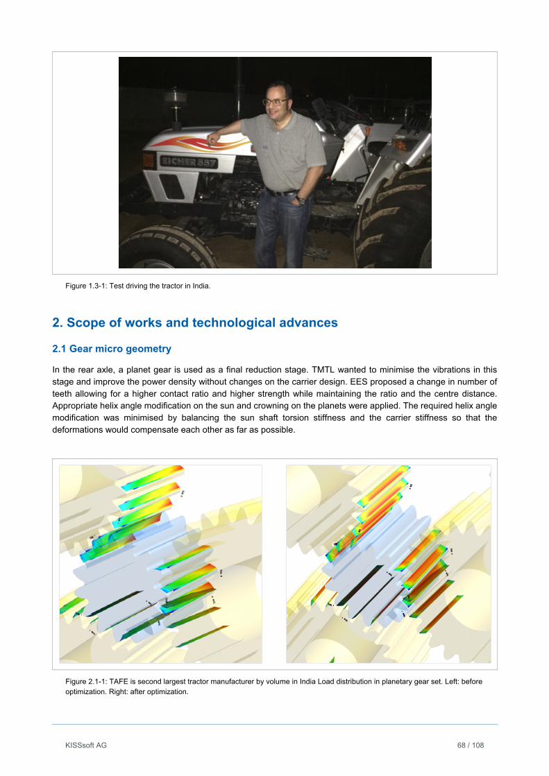
KISSsoft AG 68 / 108
Figure 1.3-1: Test driving the tractor in India.
2. Scope of works and technological advances
2.1 Gear micro geometry
In the rear axle, a planet gear is used as a final reduction stage. TMTL wanted to minimise the vibrations in this stage and improve the power density without changes on the carrier design. EES proposed a change in number of teeth allowing for a higher contact ratio and higher strength while maintaining the ratio and the centre distance. Appropriate helix angle modification on the sun and crowning on the planets were applied. The required helix angle modification was minimised by balancing the sun shaft torsion stiffness and the carrier stiffness so that the deformations would compensate each other as far as possible.
Figure 2.1-1: TAFE is second largest tractor manufacturer by volume in India Load distribution in planetary gear set. Left: before optimization. Right: after optimization.
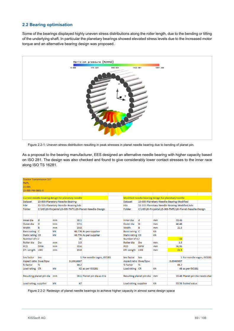
KISSsoft AG 69 / 108
2.2 Bearing optimisation
Some of the bearings displayed highly uneven stress distributions along the roller length, due to the bending or tilting of the underlying shaft. In particular the planetary bearings showed elevated stress levels due to the increased motor torque and an alternative bearing design was proposed.
Figure 2.2-1: Uneven stress distribution resulting in peak stresses in planet needle bearing due to bending of planet pin.
As a proposal to the bearing manufacturer, EES designed an alternative needle bearing with higher capacity based on ISO 281. The design was also checked and found to give considerably lower contact stresses to the inner race along ISO TS 16281.
Figure 2.2-2: Redesign of planet needle bearings to achieve higher capacity in almost same design space
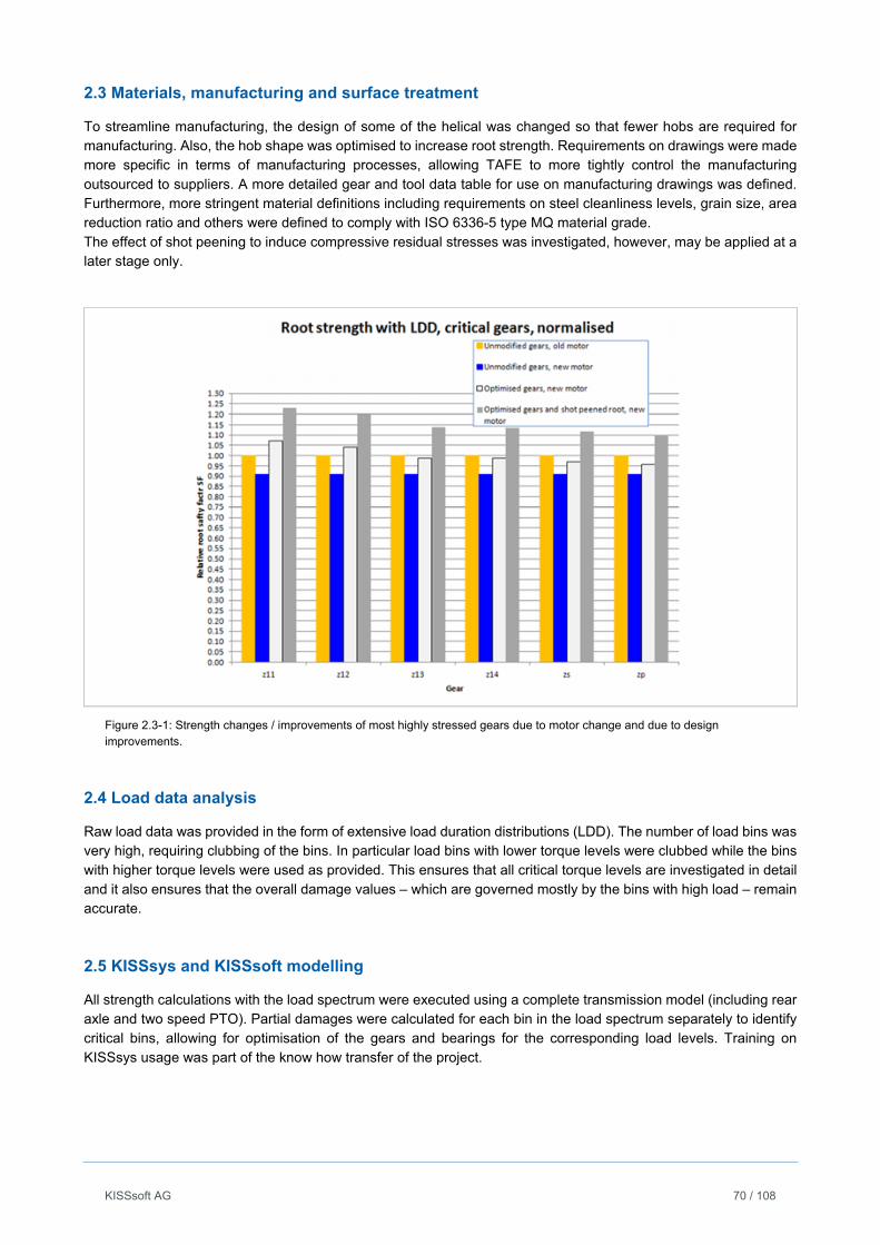
KISSsoft AG 70 / 108
2.3 Materials, manufacturing and surface treatment
To streamline manufacturing, the design of some of the helical was changed so that fewer hobs are required for manufacturing. Also, the hob shape was optimised to increase root strength. Requirements on drawings were made more specific in terms of manufacturing processes, allowing TAFE to more tightly control the manufacturing outsourced to suppliers. A more detailed gear and tool data table for use on manufacturing drawings was defined. Furthermore, more stringent material definitions including requirements on steel cleanliness levels, grain size, area reduction ratio and others were defined to comply with ISO 6336-5 type MQ material grade. The effect of shot peening to induce compressive residual stresses was investigated, however, may be applied at a later stage only.
Figure 2.3-1: Strength changes / improvements of most highly stressed gears due to motor change and due to design improvements.
2.4 Load data analysis
Raw load data was provided in the form of extensive load duration distributions (LDD). The number of load bins was very high, requiring clubbing of the bins. In particular load bins with lower torque levels were clubbed while the bins with higher torque levels were used as provided. This ensures that all critical torque levels are investigated in detail and it also ensures that the overall damage values – which are governed mostly by the bins with high load – remain accurate.
2.5 KISSsys and KISSsoft modelling
All strength calculations with the load spectrum were executed using a complete transmission model (including rear axle and two speed PTO). Partial damages were calculated for each bin in the load spectrum separately to identify critical bins, allowing for optimisation of the gears and bearings for the corresponding load levels. Training on KISSsys usage was part of the know how transfer of the project.
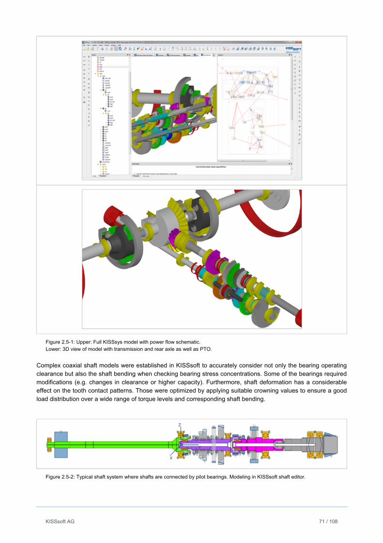
KISSsoft AG 71 / 108
Figure 2.5-1: Upper: Full KISSsys model with power flow schematic. Lower: 3D view of model with transmission and rear axle as well as PTO.
Complex coaxial shaft models were established in KISSsoft to accurately consider not only the bearing operating clearance but also the shaft bending when checking bearing stress concentrations. Some of the bearings required modifications (e.g. changes in clearance or higher capacity). Furthermore, shaft deformation has a considerable effect on the tooth contact patterns. Those were optimized by applying suitable crowning values to ensure a good load distribution over a wide range of torque levels and corresponding shaft bending.
Figure 2.5-2: Typical shaft system where shafts are connected by pilot bearings. Modeling in KISSsoft shaft editor.
KISSsoft AG 72 / 108
3. Conclusion
The project was as challenging as any tractor transmission project, covering aspects of load data synthesis, gear manufacturing, bevel gear technology, planetary gear tooth contact analysis and software training. Key to the success was an efficient communication. “We managed to fit a new motor with considerably higher torque to the existing transmission with changing only gear geometry, some technology parameters and controlling some machining parameters more closely from design side. Also, some bearings required changed or we designed them ourselves. Thanks to EES we are now also changing our drawing templates and are monitoring tool data more closely as we have seen how important this is on the gear design. We were most happy with the speedy response and technical insights shared and hope to do further projects with Mr. Hanspeter in the future”. M. D. Shelar, Chief Engineer Transmission R&D, Eicher Tractors “Working on tractor transmissions is always fun and challenging, there is no other vehicle having that many gears in such a small space. Also, looking at cylindrical, planetary and bevel gear at the same time reminds us of how important the manufacturing aspects are, they are always different for these three types of gears. I trust I was able to calculate awareness of the influence of manufacturing on design and vice versa. Working with TMTL team was refreshing and I enjoyed the interaction much, especially the test drive!” H. Dinner, EES KISSsoft GmbH Copyright Note: Any and all information contained in this report, in particular the product photographs and images, are property of TAFE TMTL and under their copyright. Above photos and images may not be reproduced without prior written agreement by TAFE TMTL.
KISSsoft AG 73 / 108
Wear on gears: Prediction of the worn tooth form and the consequences on NVH and lifetime
Dr.-Ing. Ulrich Kissling, KISSsoft AG, Bubikon, Switzerland
MSc. Ing. ETH Sandro Hauri, KISSsoft AG, Bubikon, Switzerland
Abstract
The phenomenon known as “wear” or "cold wear" experienced by plastic and metal gears is a criterion for failure. Although this topic has been noted in German technical literature since long time, no usable indications about how to calculate the risk of wear in practical applications have yet been given. When compared with the exhaustive investigations carried out on other phenomena such as bending, pitting or scuffing, it seems that wear has literally been left out in the cold! But despite this, there are applications in heavy steel gear applications where cold wear is a criterion which cannot be ignored. In a specific area of application, wear is a very important topic: for dry running plastic gears. Dry running plastic gears fail most probably through two criteria: Either by melting, because of a too high increase of the gear body temperature, or by wear. Over the past few years, the authors have worked closely with a number of manufacturers of plastic gears to investigate the problems of gear wear in detail. Together they have developed a calculation method that can be used to predict where and when local wear will occur on a tooth flank. Part of these findings have also just been published in the final version of VDI 2736 [1]. The basic mechanics of wear for lubricated, slow-running, metal gears is the same as for dry-running plastic gears. However, the wear coefficients to be applied in each case are very different and the influence of the lubricant (in particular the effect of the lubricant additives) is crucial. In 1980, at the FZG in Munich, Germany, Plewe published investigations of the wear behavior of lubricated metal gears. If the wear coefficient is known, the distribution of wear can be calculated over the tooth contact area in the contact analysis. The progress of wear must be calculated step by step because the tooth form changes as it becomes worn, and therefore the load distribution will change across the meshing. Useful results can be achieved by running the calculation with a sufficient number of small increments. Comparing the results with different measurements on metal and on plastic gears gives good matching of the results. If the step-by-step change of the tooth flank due to wear is used, the progress of different important gear characteristics as the transmission error (PPTE), the load distribution or the tooth bending stress can be investigated. The transmission error is typically decreasing during a running-in period, but tends to reach a much higher level with on-going wear. The bending stress in the tooth root will slowly increase due to the reduced tooth thickness and an increase of the notch effect due to the wear. This permits a prognostic of life expectancy until the fracture of the tooth. The load distribution over the face width is improved through wear, as long as the wear is not excessively high. This new calculation method permits therefore not only to predict the modification of the tooth contact area through wear, but to predict also the consequences on the gear behavior.
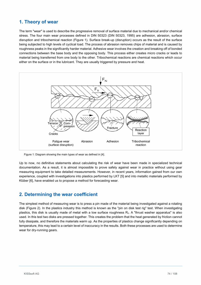
KISSsoft AG 74 / 108
1. Theory of wear
The term "wear" is used to describe the progressive removal of surface material due to mechanical and/or chemical stress. The four main wear processes defined in DIN 50323 (DIN 50323, 1995) are adhesion, abrasion, surface disruption and tribochemical reaction (Figure 1). Surface break-up (disruption) occurs as the result of the surface being subjected to high levels of cyclical load. The process of abrasion removes chips of material and is caused by roughness peaks in the significantly harder material. Adhesive wear involves the creation and breaking off of bonded connections between the base body and the opposing body. This process either creates micro cracks or leads to material being transferred from one body to the other. Tribochemical reactions are chemical reactions which occur either on the surface or in the lubricant. They are usually triggered by pressure and heat.
Figure 1: Diagram showing the main types of wear as defined in [4].
Up to now, no definitive statements about calculating the risk of wear have been made in specialized technical documentation. As a result, it is almost impossible to prove safety against wear in practice without using gear measuring equipment to take detailed measurements. However, in recent years, information gained from our own experience, coupled with investigations into plastics performed by LKT [5] and into metallic materials performed by Klüber [6], have enabled us to propose a method for forecasting wear.
2. Determining the wear coefficient
The simplest method of measuring wear is to press a pin made of the material being investigated against a rotating disk (Figure 2). In the plastics industry this method is known as the "pin on disk test rig" test. When investigating plastics, this disk is usually made of metal with a low surface roughness Rz. A "thrust washer apparatus" is also used. In this test two disks are pressed together. This creates the problem that the heat generated by friction cannot fully dissipate, and therefore the materials warm up. As the properties of plastics change significantly depending on temperature, this may lead to a certain level of inaccuracy in the results. Both these processes are used to determine wear for dry-running gears.
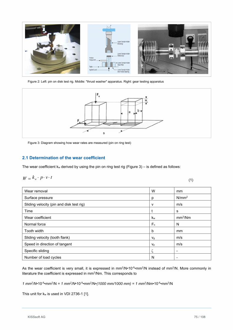
KISSsoft AG 75 / 108
Figure 2: Left: pin on disk test rig. Middle: "thrust washer" apparatus. Right: gear testing apparatus
Figure 3: Diagram showing how wear rates are measured (pin on ring test)
2.1 Determination of the wear coefficient
The wear coefficient kw derived by using the pin on ring test rig (Figure 3) – is defined as follows:
W tvpkw (1)
Wear removal W mm
Surface pressure p N/mm2
Sliding velocity (pin and disk test rig) v m/s
Time t s
Wear coefficient kw mm3/Nm
Normal force Fn N
Tooth width b mm
Sliding velocity (tooth flank) vg m/s
Speed in direction of tangent vp m/s
Specific sliding -
Number of load cycles N -
As the wear coefficient is very small, it is expressed in mm2/N•10-9•mm2/N instead of mm2/N. More commonly in literature the coefficient is expressed in mm3/Nm. This corresponds to 1 mm2/N•10-9•mm2/N = 1 mm2/N•10-9•mm2/N•(1000 mm/1000 mm) = 1 mm3/Nm•10-6•mm3/N This unit for kw is used in VDI 2736-1 [1].
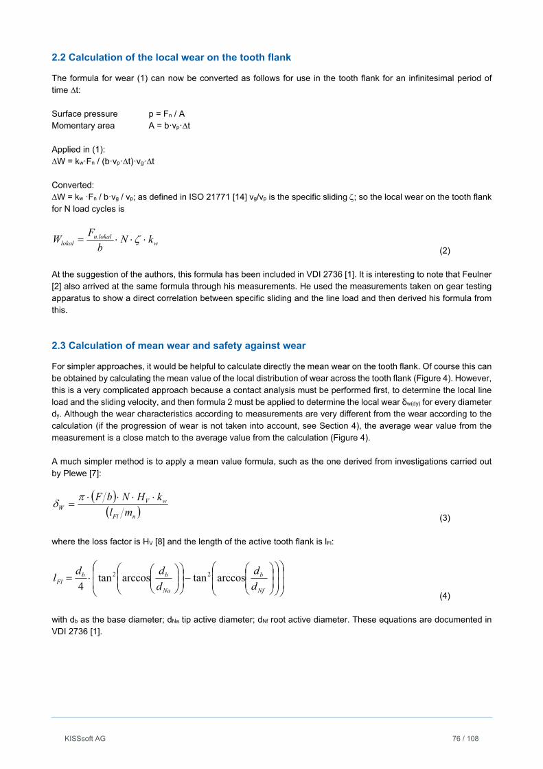
KISSsoft AG 76 / 108
2.2 Calculation of the local wear on the tooth flank
The formula for wear (1) can now be converted as follows for use in the tooth flank for an infinitesimal period of time ∆t: Surface pressure p = Fn / A Momentary area A = b·vp·∆t Applied in (1): ∆W = kw·Fn / (b·vp·∆t)·vg·∆t Converted: ∆W = kw ·Fn / b·vg / vp; as defined in ISO 21771 [14] vg/vp is the specific sliding ; so the local wear on the tooth flank for N load cycles is
wlokaln
lokal kNb
FW .
(2) At the suggestion of the authors, this formula has been included in VDI 2736 [1]. It is interesting to note that Feulner [2] also arrived at the same formula through his measurements. He used the measurements taken on gear testing apparatus to show a direct correlation between specific sliding and the line load and then derived his formula from this.
2.3 Calculation of mean wear and safety against wear
For simpler approaches, it would be helpful to calculate directly the mean wear on the tooth flank. Of course this can be obtained by calculating the mean value of the local distribution of wear across the tooth flank (Figure 4). However, this is a very complicated approach because a contact analysis must be performed first, to determine the local line load and the sliding velocity, and then formula 2 must be applied to determine the local wear δw(dy) for every diameter dy. Although the wear characteristics according to measurements are very different from the wear according to the calculation (if the progression of wear is not taken into account, see Section 4), the average wear value from the measurement is a close match to the average value from the calculation (Figure 4). A much simpler method is to apply a mean value formula, such as the one derived from investigations carried out by Plewe [7]:
nFl
wVW ml
kHNbF
(3) where the loss factor is HV [8] and the length of the active tooth flank is lFl:
Nf
b
Na
bbFl d
d
d
ddl arccostanarccostan
422
(4) with db as the base diameter; dNa tip active diameter; dNf root active diameter. These equations are documented in VDI 2736 [1].
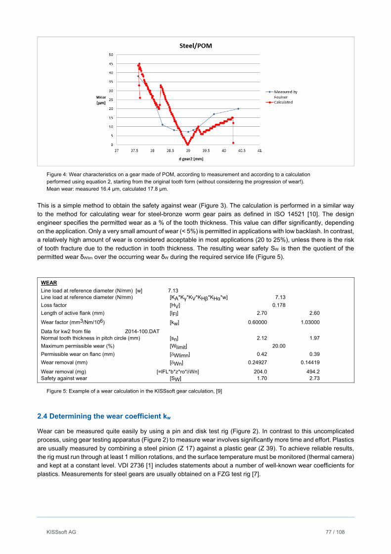
KISSsoft AG 77 / 108
Figure 4: Wear characteristics on a gear made of POM, according to measurement and according to a calculation performed using equation 2, starting from the original tooth form (without considering the progression of wear!). Mean wear: measured 16.4 μm, calculated 17.8 μm.
This is a simple method to obtain the safety against wear (Figure 3). The calculation is performed in a similar way to the method for calculating wear for steel-bronze worm gear pairs as defined in ISO 14521 [10]. The design engineer specifies the permitted wear as a % of the tooth thickness. This value can differ significantly, depending on the application. Only a very small amount of wear (< 5%) is permitted in applications with low backlash. In contrast, a relatively high amount of wear is considered acceptable in most applications (20 to 25%), unless there is the risk of tooth fracture due to the reduction in tooth thickness. The resulting wear safety SW is then the quotient of the permitted wear δWlim over the occurring wear δW during the required service life (Figure 5).
WEAR
Line load at reference diameter (N/mm) [w] 7.13 Line load at reference diameter (N/mm) [KA*Kγ*KV*KHβ*KHα*w] 7.13
Loss factor [HV] 0.178
Length of active flank (mm) [lFl] 2.70 2.60
Wear factor (mm3/Nm/106) [kw] 0.60000 1.03000
Data for kw2 from file Z014-100.DAT Normal tooth thickness in pitch circle (mm) [sn] 2.12 1.97
Maximum permissible wear (%) [Wlimit] 20.00
Permissible wear on flanc (mm) [Wlimn] 0.42 0.39
Wear removal (mm) [Wn] 0.24927 0.14419
Wear removal (mg) [=lFL*b*z*ro*Wn] 204.0 494.2 Safety against wear [SW] 1.70 2.73
Figure 5: Example of a wear calculation in the KISSsoft gear calculation, [9]
2.4 Determining the wear coefficient kw
Wear can be measured quite easily by using a pin and disk test rig (Figure 2). In contrast to this uncomplicated process, using gear testing apparatus (Figure 2) to measure wear involves significantly more time and effort. Plastics are usually measured by combining a steel pinion (Z 17) against a plastic gear (Z 39). To achieve reliable results, the rig must run through at least 1 million rotations, and the surface temperature must be monitored (thermal camera) and kept at a constant level. VDI 2736 [1] includes statements about a number of well-known wear coefficients for plastics. Measurements for steel gears are usually obtained on a FZG test rig [7].

KISSsoft AG 78 / 108
The decisive issue in being able to determine coefficients that are as time- and cost-effective as possible, is to ascertain whether measurements taken using the pin and disk test rig achieve similar wear properties to measurements taken by the gear testing apparatus. Although Feulner's [2] investigations into plastic gears do not address this issue, he has published measurement data from which a solution can be derived.
Material pairing Data
Gear test rig
kw
Gear test rig
Data
Pin and
disk
test rig
kw
Pin and disk
test rig
kw
Pin and disk
test rig
at Rz
0.45 m *
Steel/POM 1500-3000 rpm
Rz 0.45 m
1.03-1.34 vg 0.5 m/s
Rz 1.5 m
3.4 1.0
Steel/PBT As above 3.66-3.69 As above 7.8 n/a
* Estimated in accordance with the surface roughness shown in Figure 3.2 in [4]
Figure 6: A comparison of the wear coefficients, determined using a gear test rig and a pin and disk test rig.
The values from the pin and disk test rig are greater by a factor of approximately 2 (Figure 6). The difference is probably due to the surface roughness. The roughness Rz (pin and disk) of 1.5 μm to Rz (test rig) of 0.45 μm has a significant effect, as shown in Figure 6. As shown in the diagram from Feulner, kw for POM at Rz =0.45 μm is approximately 3 times greater than at Rz =1.5 μm. When converted, this would result in approximately 1.0 mm3/Nm 10-6 which would be quite a good match. In any case, measuring the wear coefficient using the pin and disk test rig achieves results that are of the correct order of magnitude. It must not be forgotten that a difference of "only" a factor of 2 between the measured coefficients is actually a good result because it can be used to estimate the service life to an accuracy of +-50%. This is a major improvement when compared with previous options which only enabled a very rough estimate of service life (with variations of 500% or more). Still it is quite obvious that these relationships must be investigated in greater detail in future. As yet, no data is available about whether a measurement taken using a pin and disk test rig can be used to determine useful values for measuring the wear coefficients of metallic materials. It is probable that this method can be used for weak metal materials in dry-running gears. However, if the effect of lubricants are to be considered when measuring wear coefficients, it is almost certain that gear testing apparatus must be used.
2.5 Lubrication
It is well known from many applications that wear happens only in not lubricated reducers. Oil lubricated gears normally fail by root fracture. If a bit of oil is involved, wear can be observed only in rare cases. Recently Fürstenberger [11] measured the wear rate on a PA12 spur gear meshing with a steel gear. The results (table 1)

KISSsoft AG 79 / 108
show that the wear coefficient in an oil bath is about 30 times lower than when dry-running. This not surprising, but confirming the expectations. But only few gearboxes with plastic gears are oil lubricated, normally grease is used. With grease a prognostic is more difficult, because the conditions during the life cycle of the gear-reducer can change heavily. In one case the grease will remain in the tooth meshing (where it should be) and therefore the operating condition is similar to an oil lubrication. In another case the grease migth be distributed on the gearbox wall and no grease will remain on the gear, so the gear mesh will become similar to a dry running gear.
Lubrication Wear coefficient kw, mm3/Nm•1e-6
Dry running 4.20
Grease 0.30
Oil 0.14
Table 1: Wear coefficient kw for PA12, deduced from wear rates as measured by [11, fig.8.9, p. 110]
Therefore grease lubricated gears will have a wear coefficient which is in between the oil- and the dry-running-coefficient. But still in most cases grease lubricated reducers do have a low risk of wear.
3. Determining the Progression of Wear
The course of the wear distribution can be calculated by applying the formula for local wear on the flank in a gear contact analysis. This makes it possible to determine the shape of the abraded tooth flank. Initially this approach did not provide any usable results, if the wear, starting with a perfect tooth form, was determined in a single calculation step. The wear distribution must be calculated step by step because the tooth form changes as it becomes worn, and therefore the load distribution will change across the meshing. The algorithm is implemented in the loaded tooth contact analysis (LTCA) of KISSsoft [9]. After some preliminary tests, very useful results can now be achieved by running the calculation at a sufficient number of small increments. The maximum permitted wear per iterative step must be defined so that the iterative progression of wear can be calculated. This predefined value is critical for achieving realistic results. If the permitted level of wear per step is too high, then the number of steps needed to achieve the end result is too small and the abraded tooth form may be very different from the actual progression of wear. If the predefined value is too small, then too many steps are required. The calculation will not only take too long, but also not achieve a better result. Excellent results can usually be achieved with intervals of approximately 1 μm per mm normal module. This recently developed calculation method has been compared to a range of gears that have been subjected to testing and then measured in 3D. Figure 7 shows this type of comparison using a pairing where the plastic (PBT) output gear is badly worn. The difference between the arithmetical forecasts, with and without iterative calculation, clearly shows that the wear distribution along the flank without iteration cannot be used and displays quite a different trend to the measured progression. A maximum interval of 1μm wear per iterative step has been defined for the wear forecast with iteration. The result shows a relatively good match with the measurement.
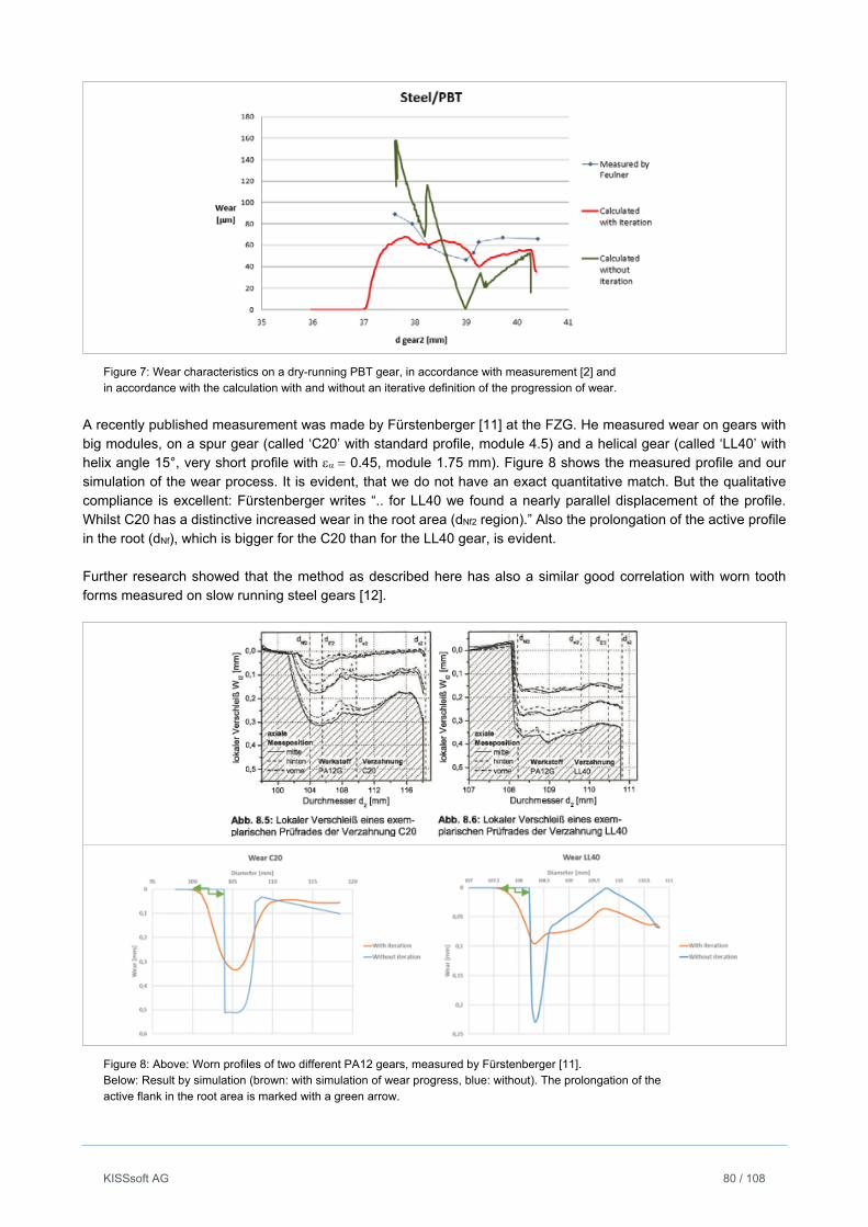
KISSsoft AG 80 / 108
Figure 7: Wear characteristics on a dry-running PBT gear, in accordance with measurement [2] and in accordance with the calculation with and without an iterative definition of the progression of wear.
A recently published measurement was made by Fürstenberger [11] at the FZG. He measured wear on gears with big modules, on a spur gear (called ‘C20’ with standard profile, module 4.5) and a helical gear (called ‘LL40’ with helix angle 15°, very short profile with 0.45, module 1.75 mm). Figure 8 shows the measured profile and our simulation of the wear process. It is evident, that we do not have an exact quantitative match. But the qualitative compliance is excellent: Fürstenberger writes “.. for LL40 we found a nearly parallel displacement of the profile. Whilst C20 has a distinctive increased wear in the root area (dNf2 region).” Also the prolongation of the active profile in the root (dNf), which is bigger for the C20 than for the LL40 gear, is evident. Further research showed that the method as described here has also a similar good correlation with worn tooth forms measured on slow running steel gears [12].
Figure 8: Above: Worn profiles of two different PA12 gears, measured by Fürstenberger [11]. Below: Result by simulation (brown: with simulation of wear progress, blue: without). The prolongation of the active flank in the root area is marked with a green arrow.
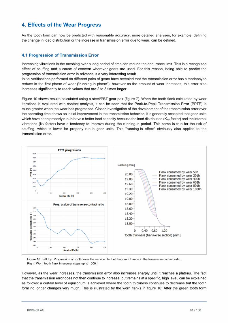
KISSsoft AG 81 / 108
4. Effects of the Wear Progress
As the tooth form can now be predicted with reasonable accuracy, more detailed analyses, for example, defining the change in load distribution or the increase in transmission error due to wear, can be defined.
4.1 Progression of Transmission Error
Increasing vibrations in the meshing over a long period of time can reduce the endurance limit. This is a recognized effect of scuffing and a cause of concern wherever gears are used. For this reason, being able to predict the progression of transmission error in advance is a very interesting result. Initial verifications performed on different pairs of gears have revealed that the transmission error has a tendency to reduce in the first phase of wear ("running-in phase"), however as the amount of wear increases, this error also increases significantly to reach values that are 2 to 3 times larger. Figure 10 shows results calculated using a steel/PBT gear pair (figure 7). When the tooth flank calculated by wear iterations is evaluated with contact analysis, it can be seen that the Peak-to-Peak Transmission Error (PPTE) is much greater when the wear has progressed. Closer investigation of the development of the transmission error over the operating time shows an initial improvement in the transmission behavior. It is generally accepted that gear units which have been properly run-in have a better load capacity because the load distribution (KH factor) and the internal vibrations (KV factor) have a tendency to improve during the running-in period. This same is true for the risk of scuffing, which is lower for properly run-in gear units. This "running-in effect" obviously also applies to the transmission error.
Figure 10: Left top: Progression of PPTE over the service life. Left bottom: Change in the transverse contact ratio. Right: Worn tooth flank in several steps up to 1000 h
However, as the wear increases, the transmission error also increases sharply until it reaches a plateau. The fact that the transmission error does not then continue to increase, but remains at a specific, high level, can be explained as follows: a certain level of equilibrium is achieved where the tooth thickness continues to decrease but the tooth form no longer changes very much. This is illustrated by the worn flanks in figure 10: After the green tooth form
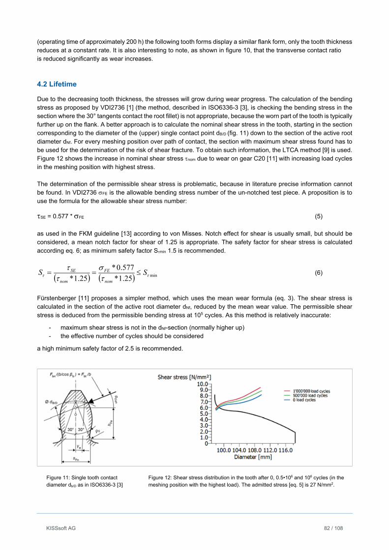
KISSsoft AG 82 / 108
(operating time of approximately 200 h) the following tooth forms display a similar flank form, only the tooth thickness reduces at a constant rate. It is also interesting to note, as shown in figure 10, that the transverse contact ratio �� is reduced significantly as wear increases.
4.2 Lifetime
Due to the decreasing tooth thickness, the stresses will grow during wear progress. The calculation of the bending stress as proposed by VDI2736 [1] (the method, described in ISO6336-3 [3], is checking the bending stress in the section where the 30° tangents contact the root fillet) is not appropriate, because the worn part of the tooth is typically further up on the flank. A better approach is to calculate the nominal shear stress in the tooth, starting in the section corresponding to the diameter of the (upper) single contact point dB/D (fig. 11) down to the section of the active root diameter dNf. For every meshing position over path of contact, the section with maximum shear stress found has to be used for the determination of the risk of shear fracture. To obtain such information, the LTCA method [9] is used. Figure 12 shows the increase in nominal shear stress nom due to wear on gear C20 [11] with increasing load cycles in the meshing position with highest stress. The determination of the permissible shear stress is problematic, because in literature precise information cannot be found. In VDI2736 FE is the allowable bending stress number of the un-notched test piece. A proposition is to use the formula for the allowable shear stress number:
SE = 0.577 * FE (5)
as used in the FKM guideline [13] according to von Misses. Notch effect for shear is usually small, but should be considered, a mean notch factor for shear of 1.25 is appropriate. The safety factor for shear stress is calculated according eq. 6; as minimum safety factor Smin 1.5 is recommended.
min25.1*
577.0*
25.1*
SSnom
FE
nom
SE (6)
Fürstenberger [11] proposes a simpler method, which uses the mean wear formula (eq. 3). The shear stress is calculated in the section of the active root diameter dNf, reduced by the mean wear value. The permissible shear stress is deduced from the permissible bending stress at 105 cycles. As this method is relatively inaccurate:
- maximum shear stress is not in the dNf-section (normally higher up) - the effective number of cycles should be considered
a high minimum safety factor of 2.5 is recommended.
Figure 11: Single tooth contact diameter db/D as in ISO6336-3 [3]
Figure 12: Shear stress distribution in the tooth after 0, 0.5•106 and 106 cycles (in the meshing position with the highest load). The admitted stress [eq. 5] is 27 N/mm2.
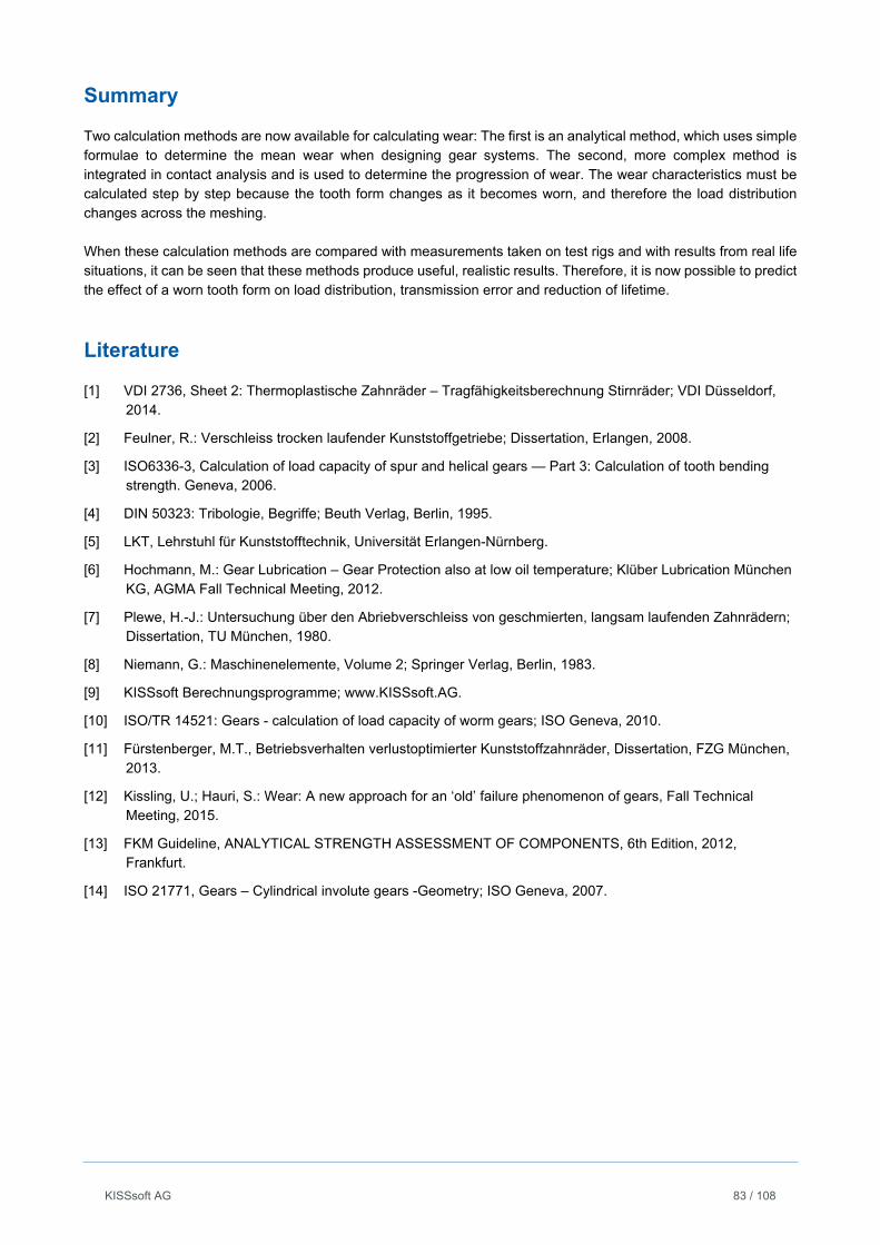
KISSsoft AG 83 / 108
Summary
Two calculation methods are now available for calculating wear: The first is an analytical method, which uses simple formulae to determine the mean wear when designing gear systems. The second, more complex method is integrated in contact analysis and is used to determine the progression of wear. The wear characteristics must be calculated step by step because the tooth form changes as it becomes worn, and therefore the load distribution changes across the meshing. When these calculation methods are compared with measurements taken on test rigs and with results from real life situations, it can be seen that these methods produce useful, realistic results. Therefore, it is now possible to predict the effect of a worn tooth form on load distribution, transmission error and reduction of lifetime.
Literature
[1] VDI 2736, Sheet 2: Thermoplastische Zahnräder – Tragfähigkeitsberechnung Stirnräder; VDI Düsseldorf, 2014.
[2] Feulner, R.: Verschleiss trocken laufender Kunststoffgetriebe; Dissertation, Erlangen, 2008.
[3] ISO6336-3, Calculation of load capacity of spur and helical gears — Part 3: Calculation of tooth bending strength. Geneva, 2006.
[4] DIN 50323: Tribologie, Begriffe; Beuth Verlag, Berlin, 1995.
[5] LKT, Lehrstuhl für Kunststofftechnik, Universität Erlangen-Nürnberg.
[6] Hochmann, M.: Gear Lubrication – Gear Protection also at low oil temperature; Klüber Lubrication München KG, AGMA Fall Technical Meeting, 2012.
[7] Plewe, H.-J.: Untersuchung über den Abriebverschleiss von geschmierten, langsam laufenden Zahnrädern; Dissertation, TU München, 1980.
[8] Niemann, G.: Maschinenelemente, Volume 2; Springer Verlag, Berlin, 1983.
[9] KISSsoft Berechnungsprogramme; www.KISSsoft.AG.
[10] ISO/TR 14521: Gears - calculation of load capacity of worm gears; ISO Geneva, 2010.
[11] Fürstenberger, M.T., Betriebsverhalten verlustoptimierter Kunststoffzahnräder, Dissertation, FZG München, 2013.
[12] Kissling, U.; Hauri, S.: Wear: A new approach for an ‘old’ failure phenomenon of gears, Fall Technical Meeting, 2015.
[13] FKM Guideline, ANALYTICAL STRENGTH ASSESSMENT OF COMPONENTS, 6th Edition, 2012, Frankfurt.
[14] ISO 21771, Gears – Cylindrical involute gears -Geometry; ISO Geneva, 2007.
KISSsoft AG 84 / 108
Accelerated testing method for polymer gears
Review of gear body temperature calculation according to VDI 2736
Dr. A. Pogačnik, Iskra Mehanizmi, Lipnica, Slovenia
Dr. J. Tavcar, Faculty of Mechanical Engineering, Ljubljana, Slovenia
Paper presented at the “International Conference on Gears 2015”
Abstract
The field of polymer gears has grown significantly in the last decade. The requirements from the industry, to design stronger, lighter, quieter and more efficient gears drives, have also motivated polymer manufacturers to produce custom made materials. These materials can have tailor made properties like low friction and wear, high dimensional stability and/or high strength. However, the use of basic polymer materials (like PA and POM) is still very common in polymer gear drives as they are tribologically compatible and have lower price compared to the tailor made polymer materials. In the last 2 years, the new VDI 2736 guideline for the design of polymer gears, was introduced. It has, compared to the old VDI 2545, an updated gear design method, but some of the limitations are still obvious. The material data for lifetime calculations is limited. In order to properly design gear drives, it seems necessary to measure the material properties and operating temperatures in gear tests prior to the gear design. The paper presents an accelerated testing procedure for plastic gears that is based on two levels of testing. 3 different materials were used for testing; POM, PA6, PA6+GF. The gears were tested at speeds between 500 rpm and 2500 rpm and torque between 0.30 Nm and 0.82 Nm. The testing procedure follows requests from product development process. The proposed method was applied in full range on gear pairs made from polyacetal (POM) and polyamide 6 (PA6). The results from lifetime testing are also compared to material properties as documented in the VDI 2736. Tests have shown that polymer gears fail in two typical ways: by root fatigue or by sudden melting. Wear fail mode can be avoided by appropriate material pair selection. Fatigue can be measured by lifetime tests and is predictable. However, melting of gears is the consequence of overload and temperature rise and is not easily predictable, because the gear temperature calculations are not completely in agreement with industrial measurements. Prediction of gear temperature is very important for polymer gears as the material properties (S-N or Wöhler curve) can depend greatly on the temperature. In some cases, even the melting of the gears can occur. Therefore, an accurate prediction of temperature in operation is necessary. The equation in VDI 2736 for the calculation of the gear temperature, contains factors, which were reviewed based on our test results. With modification of factors for the calculation of gear root temperature, a good correlation between measured and calculated root temperatures (VDI 2736) was found.
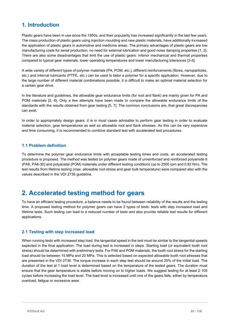
KISSsoft AG 85 / 108
1. Introduction
Plastic gears have been in use since the 1950s, and their popularity has increased significantly in the last few years. The mass production of plastic gears using injection moulding and new plastic materials, have additionally increased the application of plastic gears in automotive and medicine areas. The primary advantages of plastic gears are low manufacturing costs for serial production, no need for external lubrication and good noise damping properties [1, 2]. There are also some disadvantages that limit the use of plastic gears: inferior mechanical and thermal properties compared to typical gear materials, lower operating temperatures and lower manufacturing tolerances [3-5]. A wide variety of different types of polymer materials (PA, POM, etc.), different reinforcements (fibres, nanoparticles, etc.) and internal lubricants (PTFE, etc.) can be used to tailor a polymer for a specific application. However, due to the large number of different material combinations possible, it is difficult to make an optimal material selection for a certain gear drive. In the literature and guidelines, the allowable gear endurance limits (for root and flank) are mainly given for PA and POM materials [2, 6]. Only a few attempts have been made to compare the allowable endurance limits of the standards with the results obtained from gear testing [5, 7]. The common conclusions are, that great discrepancies can exist. In order to appropriately design gears, it is in most cases advisable to perform gear testing in order to evaluate material selection, gear temperatures as well as allowable root and flank stresses. As this can be very expensive and time consuming, it is recommended to combine standard test with accelerated test procedures.
1.1 Problem definition
To determine the polymer gear endurance limits with acceptable testing times and costs, an accelerated testing procedure is proposed. The method was tested on polymer gears made of unreinforced and reinforced polyamide 6 (PA6, PA6-30) and polyacetal (POM) materials under different testing conditions (up to 2500 rpm and 0.82 Nm). The test results from lifetime testing (max. allowable root stress and gear bulk temperature) were compared also with the values described in the VDI 2736 guideline.
2. Accelerated testing method for gears To have an efficient testing procedure, a balance needs to be found between reliability of the results and the testing time. A proposed testing method for polymer gears can have 2 types of tests: tests with step increased load and lifetime tests. Such testing can lead to a reduced number of tests and also provide reliable test results for different applications.
2.1 Testing with step increased load
When running tests with increased step load, the tangential speed in the test must be similar to the tangential speeds expected in the final application. The load during test is increased in steps. Starting load (or equivalent tooth root stress) should be determined with preliminary tests. For PA6 and POM materials, the tooth root stress for the starting load should be between 15 MPa and 20 MPa. This is selected based on expected allowable tooth root stresses that are presented in the VDI 2736. The torque increase in each step test should be around 20% of the initial load. The duration of the test at 1 load level is determined based on the temperature of the tested gears. The duration must ensure that the gear temperature is stable before moving on to higher loads. We suggest testing for at least 2·105 cycles before increasing the load level. The load level is increased until one of the gears fails, either by temperature overload, fatigue or excessive wear.
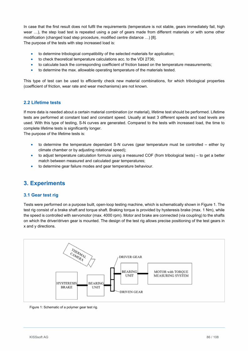
KISSsoft AG 86 / 108
In case that the first result does not fulfil the requirements (temperature is not stable, gears immediately fail, high wear …), the step load test is repeated using a pair of gears made from different materials or with some other modification (changed load step procedure, modified centre distance …) [8]. The purpose of the tests with step increased load is:
to determine tribological compatibility of the selected materials for application; to check theoretical temperature calculations acc. to the VDI 2736; to calculate back the corresponding coefficient of friction based on the temperature measurements; to determine the max. allowable operating temperature of the materials tested.
This type of test can be used to efficiently check new material combinations, for which tribological properties (coefficient of friction, wear rate and wear mechanisms) are not known.
2.2 Lifetime tests
If more data is needed about a certain material combination (or material), lifetime test should be performed. Lifetime tests are performed at constant load and constant speed. Usually at least 3 different speeds and load levels are used. With this type of testing, S-N curves are generated. Compared to the tests with increased load, the time to complete lifetime tests is significantly longer. The purpose of the lifetime tests is:
to determine the temperature dependant S-N curves (gear temperature must be controlled – either by climate chamber or by adjusting rotational speed);
to adjust temperature calculation formula using a measured COF (from tribological tests) – to get a better match between measured and calculated gear temperatures;
to determine gear failure modes and gear temperature behaviour.
3. Experiments
3.1 Gear test rig
Tests were performed on a purpose built, open-loop testing machine, which is schematically shown in Figure 1. The test rig consist of a brake shaft and torque shaft. Braking torque is provided by hysteresis brake (max. 1 Nm), while the speed is controlled with servomotor (max. 4000 rpm). Motor and brake are connected (via coupling) to the shafts on which the driver/driven gear is mounted. The design of the test rig allows precise positioning of the test gears in x and y directions.
Figure 1: Schematic of a polymer gear test rig.
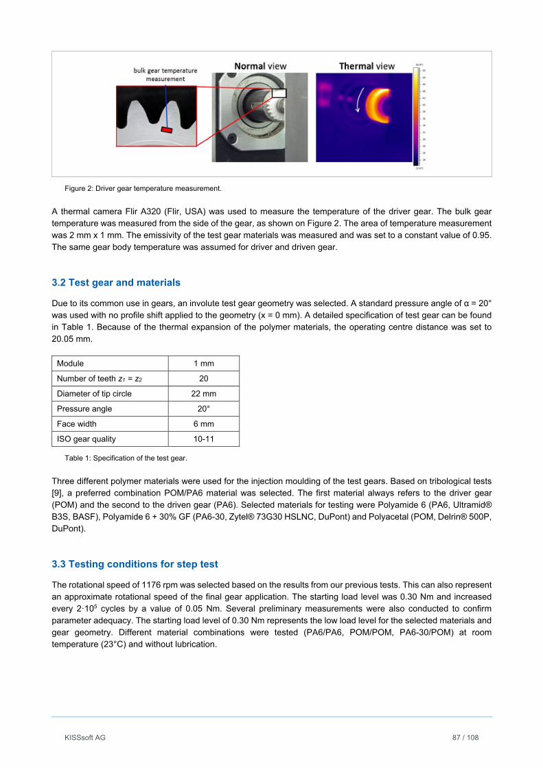
KISSsoft AG 87 / 108
Figure 2: Driver gear temperature measurement.
A thermal camera Flir A320 (Flir, USA) was used to measure the temperature of the driver gear. The bulk gear temperature was measured from the side of the gear, as shown on Figure 2. The area of temperature measurement was 2 mm x 1 mm. The emissivity of the test gear materials was measured and was set to a constant value of 0.95. The same gear body temperature was assumed for driver and driven gear.
3.2 Test gear and materials
Due to its common use in gears, an involute test gear geometry was selected. A standard pressure angle of α = 20° was used with no profile shift applied to the geometry (x = 0 mm). A detailed specification of test gear can be found in Table 1. Because of the thermal expansion of the polymer materials, the operating centre distance was set to 20.05 mm.
Module 1 mm
Number of teeth z1 = z2 20
Diameter of tip circle 22 mm
Pressure angle 20°
Face width 6 mm
ISO gear quality 10-11
Table 1: Specification of the test gear.
Three different polymer materials were used for the injection moulding of the test gears. Based on tribological tests [9], a preferred combination POM/PA6 material was selected. The first material always refers to the driver gear (POM) and the second to the driven gear (PA6). Selected materials for testing were Polyamide 6 (PA6, Ultramid® B3S, BASF), Polyamide 6 + 30% GF (PA6-30, Zytel® 73G30 HSLNC, DuPont) and Polyacetal (POM, Delrin® 500P, DuPont).
3.3 Testing conditions for step test
The rotational speed of 1176 rpm was selected based on the results from our previous tests. This can also represent an approximate rotational speed of the final gear application. The starting load level was 0.30 Nm and increased every 2·105 cycles by a value of 0.05 Nm. Several preliminary measurements were also conducted to confirm parameter adequacy. The starting load level of 0.30 Nm represents the low load level for the selected materials and gear geometry. Different material combinations were tested (PA6/PA6, POM/POM, PA6-30/POM) at room temperature (23°C) and without lubrication.
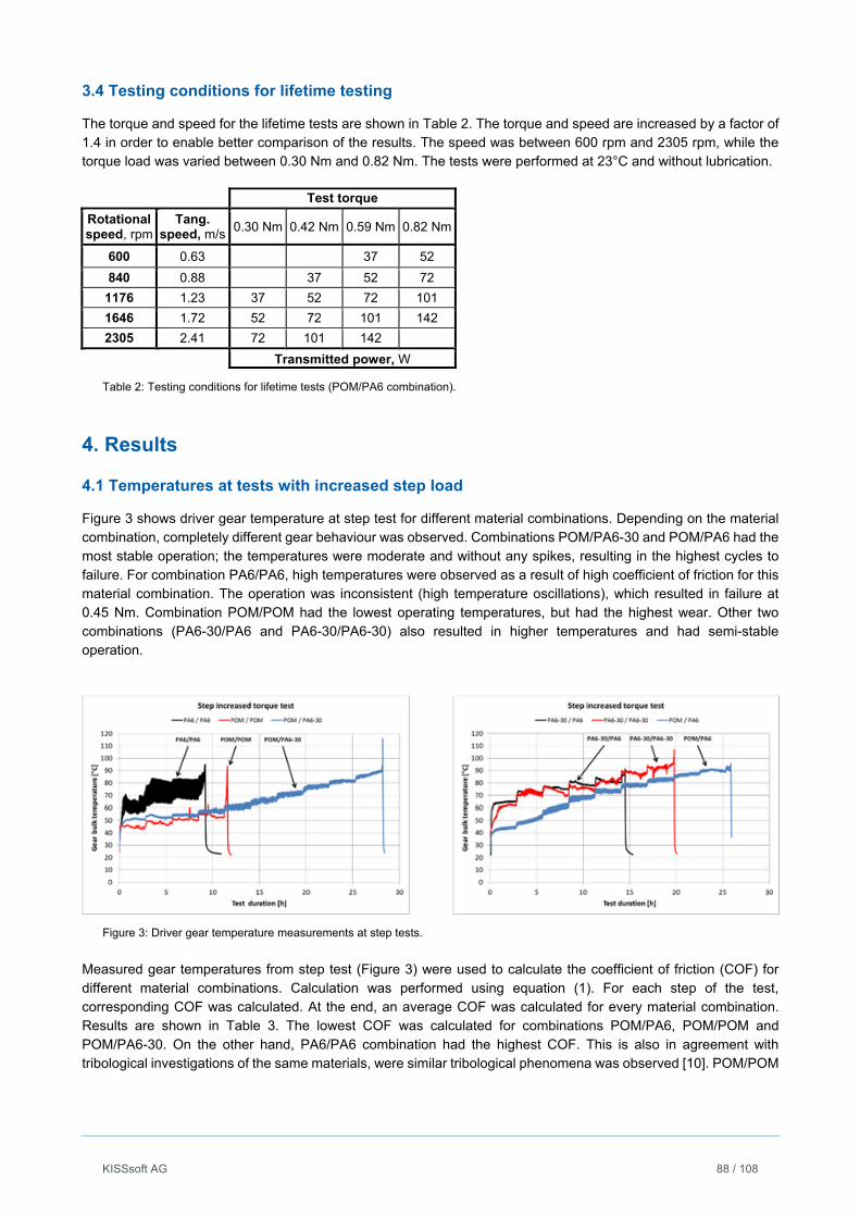
KISSsoft AG 88 / 108
3.4 Testing conditions for lifetime testing
The torque and speed for the lifetime tests are shown in Table 2. The torque and speed are increased by a factor of 1.4 in order to enable better comparison of the results. The speed was between 600 rpm and 2305 rpm, while the torque load was varied between 0.30 Nm and 0.82 Nm. The tests were performed at 23°C and without lubrication.
Test torque
Rotational speed, rpm
Tang. speed, m/s
0.30 Nm 0.42 Nm 0.59 Nm 0.82 Nm
600 0.63 37 52
840 0.88 37 52 72
1176 1.23 37 52 72 101
1646 1.72 52 72 101 142
2305 2.41 72 101 142
Transmitted power, W
Table 2: Testing conditions for lifetime tests (POM/PA6 combination).
4. Results
4.1 Temperatures at tests with increased step load
Figure 3 shows driver gear temperature at step test for different material combinations. Depending on the material combination, completely different gear behaviour was observed. Combinations POM/PA6-30 and POM/PA6 had the most stable operation; the temperatures were moderate and without any spikes, resulting in the highest cycles to failure. For combination PA6/PA6, high temperatures were observed as a result of high coefficient of friction for this material combination. The operation was inconsistent (high temperature oscillations), which resulted in failure at 0.45 Nm. Combination POM/POM had the lowest operating temperatures, but had the highest wear. Other two combinations (PA6-30/PA6 and PA6-30/PA6-30) also resulted in higher temperatures and had semi-stable operation.
Figure 3: Driver gear temperature measurements at step tests.
Measured gear temperatures from step test (Figure 3) were used to calculate the coefficient of friction (COF) for different material combinations. Calculation was performed using equation (1). For each step of the test, corresponding COF was calculated. At the end, an average COF was calculated for every material combination. Results are shown in Table 3. The lowest COF was calculated for combinations POM/PA6, POM/POM and POM/PA6-30. On the other hand, PA6/PA6 combination had the highest COF. This is also in agreement with tribological investigations of the same materials, were similar tribological phenomena was observed [10]. POM/POM
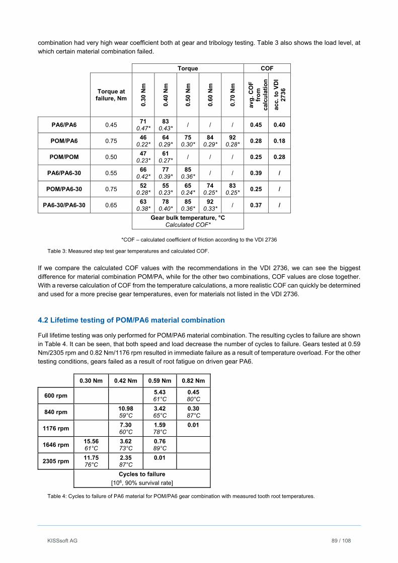
KISSsoft AG 89 / 108
combination had very high wear coefficient both at gear and tribology testing. Table 3 also shows the load level, at which certain material combination failed.
Torque COF
Torque at
failure, Nm
0.30
Nm
0.40
Nm
0.50
Nm
0.60
Nm
0.70
Nm
avg
. CO
F
fro
m
calc
ula
tio
n
acc.
to
VD
I 27
36
PA6/PA6 0.45 71
0.47* 83
0.43* / / / 0.45 0.40
POM/PA6 0.75 46
0.22* 64
0.29* 75
0.30* 84
0.29* 92
0.28* 0.28 0.18
POM/POM 0.50 47
0.23* 61
0.27* / / / 0.25 0.28
PA6/PA6-30 0.55 66
0.42* 77
0.39* 85
0.36* / / 0.39 /
POM/PA6-30 0.75 52
0.28* 55
0.23* 65
0.24* 74
0.25* 83
0.25* 0.25 /
PA6-30/PA6-30 0.65 63
0.38* 78
0.40* 85
0.36* 92
0.33* / 0.37 /
Gear bulk temperature, °C
Calculated COF*
*COF – calculated coefficient of friction according to the VDI 2736
Table 3: Measured step test gear temperatures and calculated COF.
If we compare the calculated COF values with the recommendations in the VDI 2736, we can see the biggest difference for material combination POM/PA, while for the other two combinations, COF values are close together. With a reverse calculation of COF from the temperature calculations, a more realistic COF can quickly be determined and used for a more precise gear temperatures, even for materials not listed in the VDI 2736.
4.2 Lifetime testing of POM/PA6 material combination
Full lifetime testing was only performed for POM/PA6 material combination. The resulting cycles to failure are shown in Table 4. It can be seen, that both speed and load decrease the number of cycles to failure. Gears tested at 0.59 Nm/2305 rpm and 0.82 Nm/1176 rpm resulted in immediate failure as a result of temperature overload. For the other testing conditions, gears failed as a result of root fatigue on driven gear PA6.
0.30 Nm 0.42 Nm 0.59 Nm 0.82 Nm
600 rpm 5.4361°C
0.4580°C
840 rpm 10.98 59°C
3.4265°C
0.3087°C
1176 rpm 7.30 60°C
1.5978°C
0.01
1646 rpm 15.56 61°C
3.62 73°C
0.7689°C
2305 rpm 11.75 76°C
2.35 87°C
0.01
Cycles to failure
[106, 90% survival rate]
Table 4: Cycles to failure of PA6 material for POM/PA6 gear combination with measured tooth root temperatures.
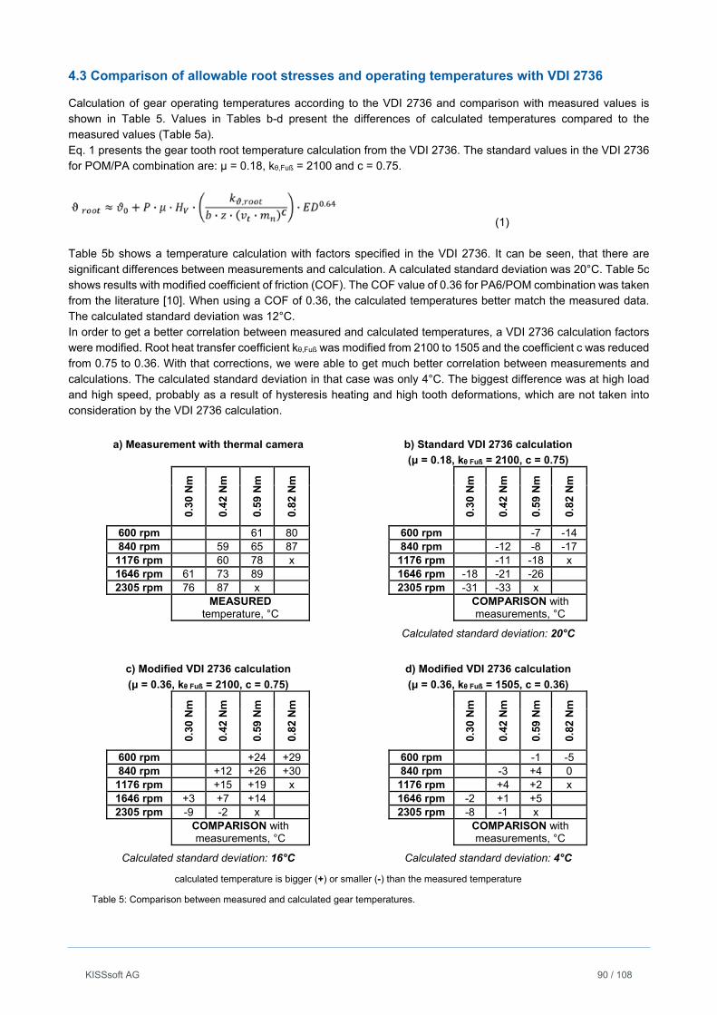
KISSsoft AG 90 / 108
4.3 Comparison of allowable root stresses and operating temperatures with VDI 2736
Calculation of gear operating temperatures according to the VDI 2736 and comparison with measured values is shown in Table 5. Values in Tables b-d present the differences of calculated temperatures compared to the measured values (Table 5a). Eq. 1 presents the gear tooth root temperature calculation from the VDI 2736. The standard values in the VDI 2736 for POM/PA combination are: μ = 0.18, kθ,Fuß = 2100 and c = 0.75.
(1) Table 5b shows a temperature calculation with factors specified in the VDI 2736. It can be seen, that there are significant differences between measurements and calculation. A calculated standard deviation was 20°C. Table 5c shows results with modified coefficient of friction (COF). The COF value of 0.36 for PA6/POM combination was taken from the literature [10]. When using a COF of 0.36, the calculated temperatures better match the measured data. The calculated standard deviation was 12°C. In order to get a better correlation between measured and calculated temperatures, a VDI 2736 calculation factors were modified. Root heat transfer coefficient kθ,Fuß was modified from 2100 to 1505 and the coefficient c was reduced from 0.75 to 0.36. With that corrections, we were able to get much better correlation between measurements and calculations. The calculated standard deviation in that case was only 4°C. The biggest difference was at high load and high speed, probably as a result of hysteresis heating and high tooth deformations, which are not taken into consideration by the VDI 2736 calculation.
a) Measurement with thermal camera
0.30
Nm
0.42
Nm
0.59
Nm
0.82
Nm
600 rpm 61 80 840 rpm 59 65 87
1176 rpm 60 78 x 1646 rpm 61 73 89 2305 rpm 76 87 x
MEASURED
temperature, °C
b) Standard VDI 2736 calculation
(μ = 0.18, kθ Fuß = 2100, c = 0.75)
0.30
Nm
0.42
Nm
0.59
Nm
0.82
Nm
600 rpm -7 -14 840 rpm -12 -8 -17
1176 rpm -11 -18 x 1646 rpm -18 -21 -26 2305 rpm -31 -33 x
COMPARISON with measurements, °C
Calculated standard deviation: 20°C
c) Modified VDI 2736 calculation
(μ = 0.36, kθ Fuß = 2100, c = 0.75)
0.30
Nm
0.42
Nm
0.59
Nm
0.82
Nm
600 rpm +24 +29 840 rpm +12 +26 +30
1176 rpm +15 +19 x 1646 rpm +3 +7 +14 2305 rpm -9 -2 x
COMPARISON with measurements, °C
Calculated standard deviation: 16°C
d) Modified VDI 2736 calculation
(μ = 0.36, kθ Fuß = 1505, c = 0.36)
0.30
Nm
0.42
Nm
0.59
Nm
0.82
Nm
600 rpm -1 -5 840 rpm -3 +4 0
1176 rpm +4 +2 x 1646 rpm -2 +1 +5 2305 rpm -8 -1 x
COMPARISON with measurements, °C
Calculated standard deviation: 4°C
calculated temperature is bigger (+) or smaller (-) than the measured temperature
Table 5: Comparison between measured and calculated gear temperatures.
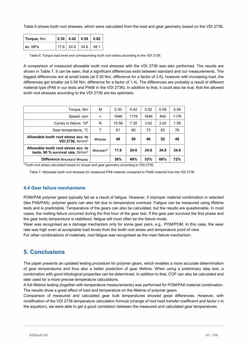
KISSsoft AG 91 / 108
Table 6 shows tooth root stresses, which were calculated from the load and gear geometry based on the VDI 2736.
Torque, Nm 0.30 0.42 0.59 0.82
σF, MPa 17.6 24.6 34.6 48.1
Table 6: Torque load level and corresponding tooth root stress according to the VDI 2736.
A comparison of measured allowable tooth root stresses with the VDI 2736 was also performed. The results are shown in Table 7. It can be seen, that a significant differences exist between standard and our measurements. The biggest differences are at small loads (at 0.30 Nm, difference for a factor of 2.6), however with increasing load, the differences get smaller (at 0.59 Nm, difference for a factor of 1.4). The differences are probably a result of different material type (PA6 in our tests and PA66 in the VDI 2736). In addition to that, it could also be true, that the allowed tooth root stresses according to the VDI 2736 are too optimistic.
Torque, Nm M 0.30 0.42 0.42 0.59 0.59
Speed, rpm v 1646 1176 1646 840 1176
Cycles to failure, 106 N 15.56 7.30 3.62 3.42 1.59
Gear temperature, °C T 61 60 73 65 78
Allowable tooth root stress acc. to VDI 2736, N/mm2
σFE(VDI) 46 50 46 52 48
Allowable tooth root stress acc. to tests, 90 % survival rate, N/mm2
σFE(TEST)* 17.6 24.6 24.6 34.6 34.6
Difference σFE(TEST)/ σFE(VDI) 38% 49% 53% 66% 72%
*Tooth root stress calculated based on torque and gear geometry according to VDI 2736.
Table 7: Allowable tooth root stresses for measured PA6 material compared to PA66 material from the VDI 2736.
4.4 Gear failure mechanisms
POM/PA6 polymer gears typically fail as a result of fatigue. However, if improper material combination in selected (like PA6/PA6), polymer gears can also fail due to temperature overload. Fatigue can be measured using lifetime tests and is predictable. Temperature of the gears can also be calculated, but the results are questionable. In most cases, the melting failure occurred during the first hour of the gear test. If the gear pair survived the first phase and the gear body temperature is stabilised, fatigue will most often be the failure mode. Wear was recognised as a damage mechanism only for some gear pairs, e.g., POM/POM. In this case, the wear rate was high even at acceptable load levels from the tooth root stress and temperature point of view. For other combinations of materials, root fatigue was recognised as the main failure mechanism.
5. Conclusions
The paper presents an updated testing procedure for polymer gears, which enables a more accurate determination of gear temperatures and thus also a better prediction of gear lifetime. When using a preliminary step test, a combination with good tribological properties can be determined. In addition to that, COF can also be calculated and later used for a more precise temperature calculations. A full lifetime testing (together with temperature measurements) was performed for POM/PA6 material combination. The results show a great effect of load and temperature on the lifetime of polymer gears. Comparison of measured and calculated gear bulk temperatures showed great differences. However, with modification of the VDI 2736 temperature calculation formula (change of root heat transfer coefficient and factor c in the equation), we were able to get a good correlation between the measured and calculated gear temperatures.
KISSsoft AG 92 / 108
When comparing measured allowable tooth root stresses with the VDI 2736, again significant differences occurred (up to 62%). The differences, however, decreased with increasing load. The differences are probably a result of different material type. In addition to that, it could also be true, that the results from the VDI 2736 are too optimistic. In our research, polymer gears typically failed either as a result of root fatigue (POM/PA6) or as a result or temperature overload. Significant wear was only observed for POM/POM material combination.
6. Literature
[1] G. Erhard. Designing with Plastics, Hanser Gardner Publications (2006).
[2] VDI 2736: 2013-2, Thermoplastische Zahnräder, Stirnradgetriebe, Tragfähigkeits-Berechnung, VDI Richtlinien, VDI-Verlag GmbH, Duesseldorf (2014).
[3] S. Senthilvelan, R. Gnanamoorthy. Effect of Rotational Speed on the Performance of Unreinforced and Glass Fiber Reinforced Nylon 6 Spur Gears, Materials and Design (2007), 28:3, 765-772.
[4] S. Senthilvelan, R. Gnanamoorthy. Effect of Gear Tooth Fillet Radius on the Performance of Injection Molded Nylon 6/6 Gears, Materials and Design (2006), 27:8, 632-639.
[5] K. Mao. A new approach for polymer composite gear design, Wear (2007), 262: 3-4, 432-441.
[6] VDI 2545, Zahnräder aus thermoplastischen Kunststoffen (1981).
[7] C.J. Hooke, K. Mao, D. Walton. Measurement and prediction of the surface temperature in polymer gears and its relation to surface wear, Journal of Tribology (1993), 115: 1, 119-124.
[8] A. Pogačnik, J. Tavcar. An accelerated multilevel test and design procedure for polymer gears, Materials and Design (2015), 65:8, 961-973.
[9] A. Pogačnik, M. Kalin. Parameters influencing the running-in and long-term tribological behaviour of polyamide (PA) against polyacetal (POM) and steel, Wear (2012), 290-291, 140–148.
[10] A. Pogačnik. Effect of physical parameters on tribological properties of polymers for gears (in Slovenian language), phD thesis, 2013.
KISSsoft AG 93 / 108
VDI 2736 – New Guideline, Old Challenges
Dr. Stefan Beermann, KISSsoft AG, Bubikon, Switzerland
Paper presented at the “International Conference on Gears 2015”
Abstract
The importance of plastic gears for modern industry has been growing every year. However, for years, the only accepted method for the design of the gears at least in the Western hemisphere, was the German guideline VDI 2545 [1]. There is no ISO, DIN or AGMA standard available for the strength analysis of plastic gears. In spite of the growing demand for refined knowledge, the research in the field of plastic gears decreased over the years. Due to internal regulations, the VDI 2545 was withdrawn some years ago. Currently the final two sheets of a new guideline to replace the old one are published, enlarging the scope by covering worm gears in addition to cylindrical gears and also defining a unique way to statistically evaluate measured material data. The enlarged scope of the new guideline VDI 2736 [2] results in a larger guideline comprised of 4 parts. The first part is available as a draft and covers general recommendations and material properties. The second and third parts are published in the final version and contain methods for the strength assessment of cylindrical gears (second part) and worm gears (third part). The fourth part defines the measurement and evaluation of material properties needed for the strength analysis. A general challenge for the design of plastic gears is a large amount of undocumented mechanical properties over a wide range of environmental conditions needed in the design process. For overcoming these problems, a special process for the design has to be applied. This presentation will introduce the guideline, explaining the main formulas and also pointing out open issues and possible misunderstandings. Finally, proposals are made for the proper and efficient application of the methods from the guideline.
Introduction
Since the VDI 2545 was well accepted in the Western hemisphere when it came to designing plastic gears, it is a fair assumption that the new guideline VDI 2736 will also find broad acceptance. Both guidelines are based on the well-known DIN 3990, a standard for the strength assessment of metal gears. However, although the DIN 3990 [3] allows an assessment on a very high certainty level, for plastic gears, the design still offers some extra challenges. The major problems arise from the lack of information regarding material properties. So, for the foreseeable future, a significant amount of experience is needed for the design of a plastic gearbox. The new guideline can soften the problem slightly, but only in some parts. The structure of the new guideline follows this insight:
Part 1
The first part of the guideline offers general information about plastic gears. A large portion is devoted to properties for typical materials used for molding gears. Of course not all possible variants can be listed, so that in these cases, where a material is not included, the guideline recommends to use the CAMPUS database, which is available for free on the internet.
KISSsoft AG 94 / 108
Gears and lubricant are based on the same base raw material (oil). Therefore, the selection of the specific plastic material versus the lubricant is of high importance. A table of possible combinations and those to be avoided offers help here.
Part 2
One of the revisited topics in the new guideline is the calculation of gear body and contact temperature. Since the temperature is a very important parameter for plastic gears, this is a central point of the method. In the old guideline, the results of the formula provided, were often far from reality. Research was conducted to find a better approach than the one from Hachmann & Strickle. This research didn’t deliver any new insights of the problem. So the committee tried to improve the old formula:
, 136 ∙ ∙ ∙15∙17100∙ ,
∙∙
6.3 ∙ .
The new one now reads
ß ∙ ∙ ∙ ß
∙ ∙ ∙ ., ∙ . .
Note that in the VDI 2545, the power P has the unit kW, in the new guideline the unit is W. The degree of tooth loss HV is calculated with
∙ 1∙
. 1
A new element in this formula is the cooling down factor . . In this ED is the power up time, relative to 10 minutes. This factor takes the fact into account that most plastic gearboxes are running in small time intervals. In spite of the effort to improve the formula, the results are (still) not satisfying. Even worse, in many cases the results are less realistic than those from the old guideline. An example measurement of a spur gear set PA66 – POM, 17 and 39 teeth, module 1.0 mm, shows a temperature of about 100°C with a torque of 1.5 Nm on the output. The calculation with the old guideline predicts a maximum temperature of 300°C. The new guidelines formula results in temperatures up to 530°C. This is a value that can’t be realistic! Our strong recommendation is to fix the temperature for the design work. Often the engineer knows, at least roughly, which temperatures occurs during operation. If there is a range of temperatures, several calculations for different temperatures should be conducted anyway. In some cases, the worst case is not the one with the higher temperature. So at least two calculations, one for the highest and one for the lowest temperature, should be conducted. In addition to the failure modes treated in the VDI 2545, the new guideline also provides a method for the prediction of wear on dry-running gears. This prediction is based on a linear increase in wear. A local value is calculated based on a measured wear coefficient, the normal line load, the specific sliding velocity and of course the number of load cycles:
, ∙ ∙ ∙ .
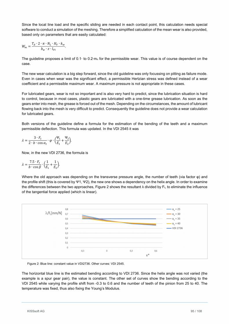
KISSsoft AG 95 / 108
Since the local line load and the specific sliding are needed in each contact point, this calculation needs special software to conduct a simulation of the meshing. Therefore a simplified calculation of the mean wear is also provided, based only on parameters that are easily calculated:
∙ 2 ∙ ∙ ∙ ∙∙ ∙
.
The guideline proposes a limit of 0.1· to 0.2·mn for the permissible wear. This value is of course dependent on the case. The new wear calculation is a big step forward, since the old guideline was only focussing on pitting as failure mode. Even in cases when wear was the significant effect, a permissible Hertzian stress was defined instead of a wear coefficient and a permissible maximum wear. A maximum pressure is not appropriate in these cases. For lubricated gears, wear is not so important and is also very hard to predict, since the lubrication situation is hard to control, because in most cases, plastic gears are lubricated with a one-time grease lubrication. As soon as the gears enter into mesh, the grease is forced out of the mesh. Depending on the circumstances, the amount of lubricant flowing back into the mesh is very difficult to predict. Consequently the guideline does not provide a wear calculation for lubricated gears. Both versions of the guideline define a formula for the estimation of the bending of the teeth and a maximum permissible deflection. This formula was updated. In the VDI 2545 it was
3 ∙2 ∙ ∙ cos
∙ ∙Ψ Ψ
.
Now, in the new VDI 2736, the formula is
7.5 ∙∙ cos
∙1 1
.
Where the old approach was depending on the transverse pressure angle, the number of teeth (via factor φ) and the profile shift (this is covered by Ψ1, Ψ2), the new one shows a dependency on the helix angle. In order to examine the differences between the two approaches, Figure 2 shows the resultant λ divided by Ft, to eliminate the influence of the tangential force applied (which is linear).
Figure 2: Blue line: constant value in VDI2736. Other curves: VDI 2545.
The horizontal blue line is the estimated bending according to VDI 2736. Since the helix angle was not varied (the example is a spur gear pair), the value is constant. The other set of curves show the bending according to the VDI 2545 while varying the profile shift from -0.3 to 0.6 and the number of teeth of the pinion from 25 to 40. The temperature was fixed, thus also fixing the Young’s Modulus.
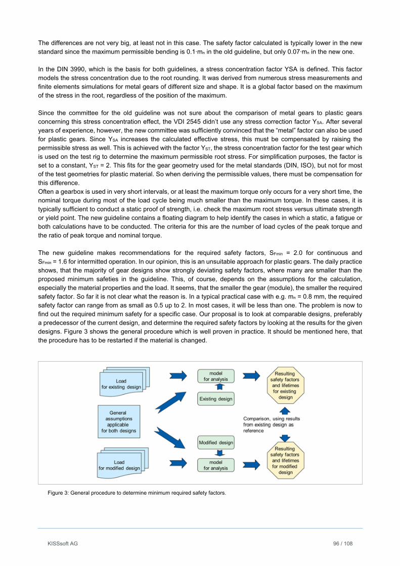
KISSsoft AG 96 / 108
The differences are not very big, at least not in this case. The safety factor calculated is typically lower in the new standard since the maximum permissible bending is 0.1·mn in the old guideline, but only 0.07·mn in the new one. In the DIN 3990, which is the basis for both guidelines, a stress concentration factor YSA is defined. This factor models the stress concentration due to the root rounding. It was derived from numerous stress measurements and finite elements simulations for metal gears of different size and shape. It is a global factor based on the maximum of the stress in the root, regardless of the position of the maximum. Since the committee for the old guideline was not sure about the comparison of metal gears to plastic gears concerning this stress concentration effect, the VDI 2545 didn’t use any stress correction factor YSA. After several years of experience, however, the new committee was sufficiently convinced that the “metal” factor can also be used for plastic gears. Since YSA increases the calculated effective stress, this must be compensated by raising the permissible stress as well. This is achieved with the factor YST, the stress concentration factor for the test gear which is used on the test rig to determine the maximum permissible root stress. For simplification purposes, the factor is set to a constant, YST = 2. This fits for the gear geometry used for the metal standards (DIN, ISO), but not for most of the test geometries for plastic material. So when deriving the permissible values, there must be compensation for this difference. Often a gearbox is used in very short intervals, or at least the maximum torque only occurs for a very short time, the nominal torque during most of the load cycle being much smaller than the maximum torque. In these cases, it is typically sufficient to conduct a static proof of strength, i.e. check the maximum root stress versus ultimate strength or yield point. The new guideline contains a floating diagram to help identify the cases in which a static, a fatigue or both calculations have to be conducted. The criteria for this are the number of load cycles of the peak torque and the ratio of peak torque and nominal torque. The new guideline makes recommendations for the required safety factors, SFmin = 2.0 for continuous and SFmin = 1.6 for intermitted operation. In our opinion, this is an unsuitable approach for plastic gears. The daily practice shows, that the majority of gear designs show strongly deviating safety factors, where many are smaller than the proposed minimum safeties in the guideline. This, of course, depends on the assumptions for the calculation, especially the material properties and the load. It seems, that the smaller the gear (module), the smaller the required safety factor. So far it is not clear what the reason is. In a typical practical case with e.g. mn = 0.8 mm, the required safety factor can range from as small as 0.5 up to 2. In most cases, it will be less than one. The problem is now to find out the required minimum safety for a specific case. Our proposal is to look at comparable designs, preferably a predecessor of the current design, and determine the required safety factors by looking at the results for the given designs. Figure 3 shows the general procedure which is well proven in practice. It should be mentioned here, that the procedure has to be restarted if the material is changed.
Figure 3: General procedure to determine minimum required safety factors.
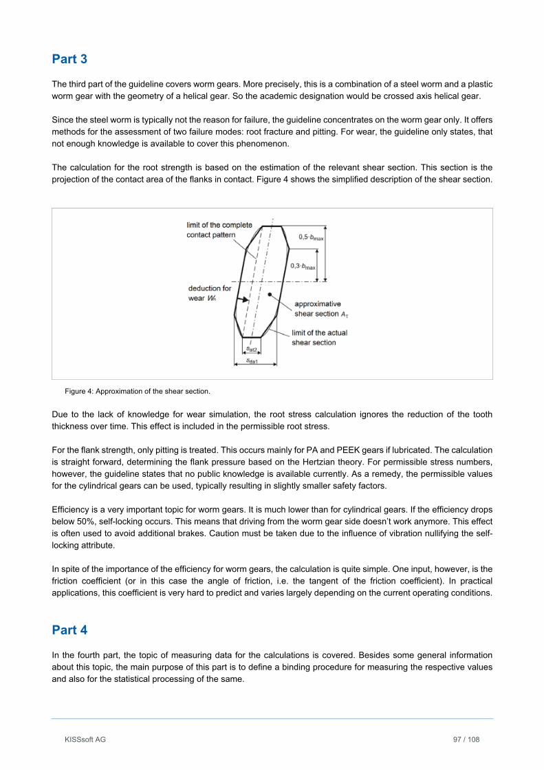
KISSsoft AG 97 / 108
Part 3
The third part of the guideline covers worm gears. More precisely, this is a combination of a steel worm and a plastic worm gear with the geometry of a helical gear. So the academic designation would be crossed axis helical gear. Since the steel worm is typically not the reason for failure, the guideline concentrates on the worm gear only. It offers methods for the assessment of two failure modes: root fracture and pitting. For wear, the guideline only states, that not enough knowledge is available to cover this phenomenon. The calculation for the root strength is based on the estimation of the relevant shear section. This section is the projection of the contact area of the flanks in contact. Figure 4 shows the simplified description of the shear section.
Figure 4: Approximation of the shear section.
Due to the lack of knowledge for wear simulation, the root stress calculation ignores the reduction of the tooth thickness over time. This effect is included in the permissible root stress. For the flank strength, only pitting is treated. This occurs mainly for PA and PEEK gears if lubricated. The calculation is straight forward, determining the flank pressure based on the Hertzian theory. For permissible stress numbers, however, the guideline states that no public knowledge is available currently. As a remedy, the permissible values for the cylindrical gears can be used, typically resulting in slightly smaller safety factors. Efficiency is a very important topic for worm gears. It is much lower than for cylindrical gears. If the efficiency drops below 50%, self-locking occurs. This means that driving from the worm gear side doesn’t work anymore. This effect is often used to avoid additional brakes. Caution must be taken due to the influence of vibration nullifying the self-locking attribute. In spite of the importance of the efficiency for worm gears, the calculation is quite simple. One input, however, is the friction coefficient (or in this case the angle of friction, i.e. the tangent of the friction coefficient). In practical applications, this coefficient is very hard to predict and varies largely depending on the current operating conditions.
Part 4
In the fourth part, the topic of measuring data for the calculations is covered. Besides some general information about this topic, the main purpose of this part is to define a binding procedure for measuring the respective values and also for the statistical processing of the same.
KISSsoft AG 98 / 108
The measurements are ideally carried out on a test rig that consists of a test gear box, a motor and brake load. The load can be implemented with a break, or by having a closed power loop with two gearboxes back-to-back. There are some alternatives for the measurement of specific failure modes. For the root stress a pulsator can be used. For wear standard models like “pin on disk” or “thrust washer test” are applied. The problem of correlating a standard three point tension bar test to the respective gear data is not yet solved, so these measurements should not be used. In addition to the general layout of the test rigs, the guideline defines three cylindrical gear pair geometries for different torque level, and one worm gear pair geometry. For the measurement of maximum permissible stress numbers for root and flank, the gear pair is run at well-defined torque and temperature values. It is very important to control the temperature directly on the gear. For the root this is typically done by inserting a sensor into the gear body, close to the root area. For the flank, non-tactile measurement is done with thermal cameras, or tactile measurement with thermal elements. The tactile measurement, however, needs to stop the gears and measure the temperature then shortly after the stop. The flanks will cool down, so the measured value must be corrected by extrapolating backwards to the start temperature when the gears were stopped. Due to the stop and the cooling down, the gears will not have a sufficiently constant temperature and the temperature can’t be controlled very well. So the approach with non-tactile measurement is recommended. A typical error, already observed several times in practice, is, that the environment temperature is controlled instead of the material temperature. Especially for non-lubricated gear sets, the material temperature can be 80°C higher, so that the material properties are measured for 100°C degrees instead of 20°C. Of course, a real gear set with an environment temperature of 20°C will also heat up. However, since most plastic gears run in intervals and have cooling down phases during their operational time, the material temperature in practical cases will hardly every meet those from a test rig, running with very constant conditions. An important topic of the fourth part is the definition of the mathematical processing of the measured data. The basic approach is to use the same formulas as defined in part 2 and 3 to determine the respective stresses. So to determine the permissible root stress, it is not the stress directly which is measured, but the torque is specified and controlled for the test. Based on this torque and the test gear geometry e.g. the root stress is calculated with
∙ ∙ ∙ Y ∙∙
.
Since we have controlled boundary conditions on a test rig the K-factors are all set to 1. The fraction YSa/YSt
compensates the simplification in part 2 with YSt = 2. This way, the real stress concentration factor is applied, and is included in the permissible stress number without the need to document it along with the material data. A second important element of the data processing is the binding method for the statistical assessment of the measured data. The measurements are triples of temperature, torque and number of load cycles until failure of the gear. The measurement of each triple has to be repeated at least three times. With the minimum of three values of load cycles, a mean variation is estimated. For a sufficient accuracy of the mean variation, a much larger number of measurements would be necessary, actually about 20 repetitions. Therefore, the values for the mean variations of all measurement points are combined to one basic mean variation, which is scaled be the number of load cycles. Based on the mean value, the number of load cycles with 10% failure probability is calculated. The prescribed procedure is a compromise between effort and accuracy. It assumes that the variation of the measurements is the same for all measured points. The assumption is based on the idea that the variation is mainly dependent on material properties and the setup of the test rig. Both are not (or better: should not be) changed during the test run over all temperatures and torque levels. From the method, some strange effects can arise. For instance a measurement, which goes to an exceptional high number of load cycles, reduces the permissible stress for all measured points, since this one measurement increases
KISSsoft AG 99 / 108
the mean variation. For the same reason it is not a good idea to just duplicate measurements in the algorithm to fulfil the need of at least three measurements per point. Since the duplicated values reduce the calculated mean variation, all permissible stress levels are increased.
Conclusions
The new guideline VDI 2736 replaces the outdated VDI 2545 in a sensible and useful way. The experiences with the old method gathered in the field over the years could mostly be considered. The extension to the worm gear drives is a huge step forward. However, some topics still remain as weak points. The modelling of the temperature is one of the more significant ones. In the current state, it is not recommendable to use the formulas from the VDI. Due to the lack of better formulae, the best way to handle the temperature in the calculations remains to assume appropriate values and in doubt make measurements on prototypes afterwards. A second point, that is still open, is the lack of availability of material data. The effort of measuring is very high and due to the large number of different plastic materials, it is not possible to only cover the most important variants completely. No solution for this is in sight, so here only measurements along specific projects can help. Hopefully, the fourth part at least better defines the measurement procedure, so that the data that was gained at such high cost can be used to the full extent. From the fact that the guideline defines minimum safety factors, problems might arise in the relationships of manufacturer and buyer of plastic gears. In many cases with the assumptions of the guideline, the minimum safety factors are not achieved. We recommend defining a way how the minimum required safety factors are determined before the start of a project in order to avoid such problems. The procedure proposed, where the minimum required safeties are found by looking at existing designs, is one way to do it and it is the way we were doing it for many years with large success. The new guideline is published in German and English. This will go a long way in helping to increase the international acceptance of the method. This is especially important for plastic gears, because this business is very international from the beginning: typical applications are in the automotive industry, the most international industry in the gear business. Also often a design is made in Europe or the USA, but the production is in Asia. Hopefully, an international discussion will result based on this guideline, eventually leading to an international standard somewhere in the future.
Literature
[1] VDI 2545:1981-01 Zahnräder aus thermoplastischen Kunststoffen. Berlin: Beuth Verlag. Withdrawn 1996-09
[2] VDI 2736:2015 Thermoplastische Zahnräder; Berlin: Beuth Verlag
[3] DIN 3990 Tragfähigkeitsberechnung von Stirnrädern. Berlin: Beuth Verlag
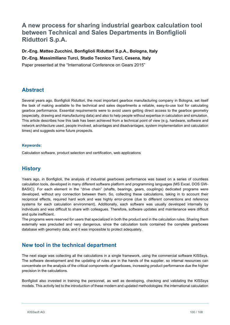
KISSsoft AG 100 / 108
A new process for sharing industrial gearbox calculation tool between Technical and Sales Departments in Bonfiglioli Riduttori S.p.A.
Dr.-Eng. Matteo Zucchini, Bonfiglioli Riduttori S.p.A., Bologna, Italy
Dr.-Eng. Massimiliano Turci, Studio Tecnico Turci, Cesena, Italy
Paper presented at the “International Conference on Gears 2015”
Abstract
Several years ago, Bonfiglioli Riduttori, the most important gearbox manufacturing company in Bologna, set itself the task of making available to the technical and sales departments a reliable, easy-to-use tool for calculating gearbox performance. Essential requirements were to avoid users getting direct access to the gearbox geometry (especially, drawing and manufacturing data) and also to help people without expertise in calculation and simulation. This article describes how this task has been achieved from a technical point of view (e.g. hardware, software and network architecture used, people involved, advantages and disadvantages, system implementation and calculation times) and suggests some future prospects.
Keywords:
Calculation software, product selection and certification, web applications
History
Years ago, in Bonfiglioli, the analysis of industrial gearboxes performance was based on a series of countless calculation tools, developed in many different software platform and programming languages (MS Excel, DOS GW-BASIC). For each element in the “drive chain” (shafts, bearings, gears, couplings) dedicated programs were developed, without any connection between them. So, collecting these calculations, taking in to account their reciprocal effects, required hard work and was highly error-prone (due to different conventions and reference systems for each calculation environment). Additionally, each software was usually developed internally by individuals and was difficult to share with colleagues. Therefore, software updates and maintenance were difficult and quite inefficient. The programs were reserved for users that specialized in both the product and in the calculation rules. Sharing them externally was precluded and very dangerous, since the calculation tools contained the complete gearboxes database with geometry data, and it was impossible to protect adequately.
New tool in the technical department
The next stage was collecting all the calculations in a single framework, using the commercial software KISSsys. The software development and the updating of rules are in the hands of the supplier, so internal resources can concentrate on the analysis of the critical components of gearboxes, increasing product performance due the higher precision in the calculations. Bonfiglioli also invested in training the personnel, as well as developing, checking and validating the KISSsys models. This activity led to the introduction of these modern and updated methodologies: the international calculation
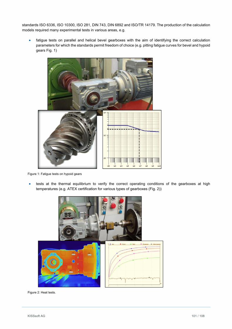
KISSsoft AG 101 / 108
standards ISO 6336, ISO 10300, ISO 281, DIN 743, DIN 6892 and ISO/TR 14179. The production of the calculation models required many experimental tests in various areas, e.g.
fatigue tests on parallel and helical bevel gearboxes with the aim of identifying the correct calculation parameters for which the standards permit freedom of choice (e.g. pitting fatigue curves for bevel and hypoid gears Fig. 1)
Figure 1: Fatigue tests on hypoid gears
tests at the thermal equilibrium to verify the correct operating conditions of the gearboxes at high
temperatures (e.g. ATEX certification for various types of gearboxes (Fig. 2))
Figure 2: Heat tests.
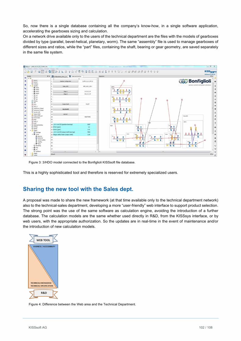
KISSsoft AG 102 / 108
So, now there is a single database containing all the company’s know-how, in a single software application, accelerating the gearboxes sizing and calculation. On a network drive available only to the users of the technical department are the files with the models of gearboxes divided by type (parallel, bevel-helical, planetary, worm). The same “assembly” file is used to manage gearboxes of different sizes and ratios, while the “part” files, containing the shaft, bearing or gear geometry, are saved separately in the same file system.
Figure 3: 3/HDO model connected to the Bonfiglioli KISSsoft file database.
This is a highly sophisticated tool and therefore is reserved for extremely specialized users.
Sharing the new tool with the Sales dept.
A proposal was made to share the new framework (at that time available only to the technical department network) also to the technical-sales department, developing a more “user-friendly” web interface to support product selection. The strong point was the use of the same software as calculation engine, avoiding the introduction of a further database. The calculation models are the same whether used directly in R&D, from the KISSsys interface, or by web users, with the appropriate authorization. So the updates are in real-time in the event of maintenance and/or the introduction of new calculation models.
Figure 4: Difference between the Web area and the Technical Department.

KISSsoft AG 103 / 108
The architecture of the system is in Fig. 4. At the bottom there is the R&D interface, containing all the details of the gearboxes (geometry, performance, etc.), which represent the company’s know-how, which must be kept confidential. At the top, on the opposite side, there is the web interface, with easy access to this protected data. The requirement of “easiness and accessibility” for the web application increases in passing from the technical area to the web area, whereas the amount of information and specific product training increase in passing from the web area to the technical area. The work-flow is represented in Fig. 5. The customer provides the salesman with the data for his application. The salesman connects to the web portal (protected by an encryption protocol) selects the most appropriate gearbox for the application, enters the data provided by the customer (torque, speed, external loads, load cycle) and then sends the calculation request to the web server. The server responds doing the calculation in a few minutes and produces a PDF file containing the results report, ready for download. The salesman can then print and deliver it to the customer with the complete offer of the most cost effective, efficient or appropriate gearbox. This architecture ensures the security of the database, since the web server, hosted in a secure area, has also the function of “pre- and post-processing”, while the client (salesman) cannot access the sensitive information (geometry, materials, etc.). The administrator, who works in the technical department, has complete control and oversight of users and their access. All of the calculations (configuration, load conditions and results) are archived on the web server, and can be eventually reloaded by the technical department for more detailed analysis (e.g. product certification). The web server database is synchronized by the server used in the technical office. The calculation models have been produced and are used inside the local corporate network, identified by the red box in fig. 5 and protected by the firewall. This process, just described in short, will be illustrated in greater depth and details in the following paragraphs.
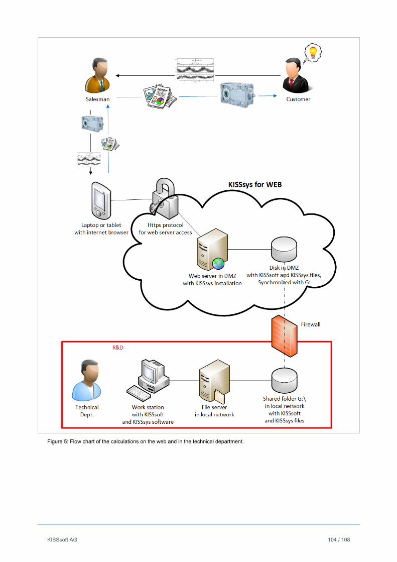
KISSsoft AG 104 / 108
Figure 5: Flow chart of the calculations on the web and in the technical department.
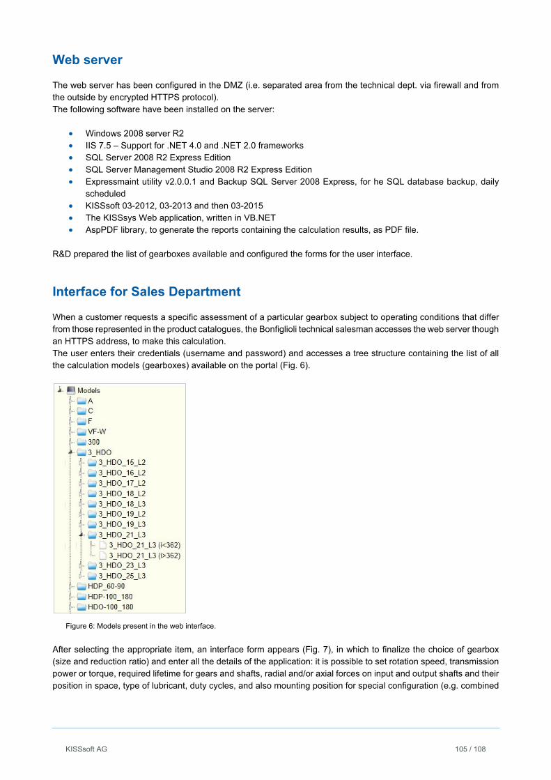
KISSsoft AG 105 / 108
Web server
The web server has been configured in the DMZ (i.e. separated area from the technical dept. via firewall and from the outside by encrypted HTTPS protocol). The following software have been installed on the server:
Windows 2008 server R2 IIS 7.5 – Support for .NET 4.0 and .NET 2.0 frameworks SQL Server 2008 R2 Express Edition SQL Server Management Studio 2008 R2 Express Edition Expressmaint utility v2.0.0.1 and Backup SQL Server 2008 Express, for he SQL database backup, daily
scheduled KISSsoft 03-2012, 03-2013 and then 03-2015 The KISSsys Web application, written in VB.NET AspPDF library, to generate the reports containing the calculation results, as PDF file.
R&D prepared the list of gearboxes available and configured the forms for the user interface.
Interface for Sales Department
When a customer requests a specific assessment of a particular gearbox subject to operating conditions that differ from those represented in the product catalogues, the Bonfiglioli technical salesman accesses the web server though an HTTPS address, to make this calculation. The user enters their credentials (username and password) and accesses a tree structure containing the list of all the calculation models (gearboxes) available on the portal (Fig. 6).
Figure 6: Models present in the web interface.
After selecting the appropriate item, an interface form appears (Fig. 7), in which to finalize the choice of gearbox (size and reduction ratio) and enter all the details of the application: it is possible to set rotation speed, transmission power or torque, required lifetime for gears and shafts, radial and/or axial forces on input and output shafts and their position in space, type of lubricant, duty cycles, and also mounting position for special configuration (e.g. combined
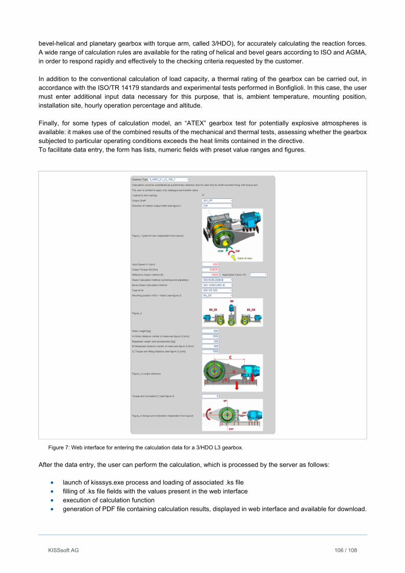
KISSsoft AG 106 / 108
bevel-helical and planetary gearbox with torque arm, called 3/HDO), for accurately calculating the reaction forces. A wide range of calculation rules are available for the rating of helical and bevel gears according to ISO and AGMA, in order to respond rapidly and effectively to the checking criteria requested by the customer. In addition to the conventional calculation of load capacity, a thermal rating of the gearbox can be carried out, in accordance with the ISO/TR 14179 standards and experimental tests performed in Bonfiglioli. In this case, the user must enter additional input data necessary for this purpose, that is, ambient temperature, mounting position, installation site, hourly operation percentage and altitude. Finally, for some types of calculation model, an “ATEX” gearbox test for potentially explosive atmospheres is available: it makes use of the combined results of the mechanical and thermal tests, assessing whether the gearbox subjected to particular operating conditions exceeds the heat limits contained in the directive. To facilitate data entry, the form has lists, numeric fields with preset value ranges and figures.
Figure 7: Web interface for entering the calculation data for a 3/HDO L3 gearbox.
After the data entry, the user can perform the calculation, which is processed by the server as follows:
launch of kisssys.exe process and loading of associated .ks file filling of .ks file fields with the values present in the web interface execution of calculation function generation of PDF file containing calculation results, displayed in web interface and available for download.
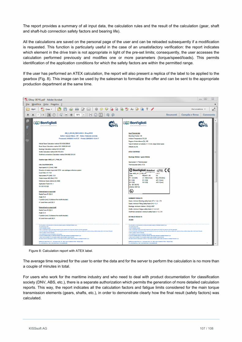
KISSsoft AG 107 / 108
The report provides a summary of all input data, the calculation rules and the result of the calculation (gear, shaft and shaft-hub connection safety factors and bearing life). All the calculations are saved on the personal page of the user and can be reloaded subsequently if a modification is requested. This function is particularly useful in the case of an unsatisfactory verification: the report indicates which element in the drive train is not appropriate in light of the pre-set limits; consequently, the user accesses the calculation performed previously and modifies one or more parameters (torque/speed/loads). This permits identification of the application conditions for which the safety factors are within the permitted range. If the user has performed an ATEX calculation, the report will also present a replica of the label to be applied to the gearbox (Fig. 8). This image can be used by the salesman to formalize the offer and can be sent to the appropriate production department at the same time.
Figure 8: Calculation report with ATEX label.
The average time required for the user to enter the data and for the server to perform the calculation is no more than a couple of minutes in total. For users who work for the maritime industry and who need to deal with product documentation for classification society (DNV, ABS, etc.), there is a separate authorization which permits the generation of more detailed calculation reports. This way, the report indicates all the calculation factors and fatigue limits considered for the main torque transmission elements (gears, shafts, etc.), in order to demonstrate clearly how the final result (safety factors) was calculated.
KISSsoft AG 108 / 108
The administrator can recall any calculation or report created by users, in order to control access, but also to refine the calculation directly on KISSsys, if necessary. This is possible thanks to the complete traceability of all calculations performed and to the synchronization of the two servers (web and R&D).
Further developments
This system, which required two years to create, is highly flexible and subject to continuous improvement and further developments, including the forthcoming smartphone App and integration with the FEM calculation in the KISSsoft environment.
Conclusions
In this way, Bonfiglioli has provided its sales network with a calculation tool featuring an accessible, effective web interface for users with less technical “expertise”, achieving the set task: calculate the gearbox rating with the same degree of detail as that carried out in the technical department, but in a simpler manner, thanks to a self explanatory, efficient, and user friendly HMI. More than 40,000 calculations were carried out in the space of about one year.
Literature
[1] www.bonfiglioli.com
[2] www.turci.biz
[3] www.kisssoft.ch
[4] www.hotminds.it