knot-logic and majorana fermions l. h. kauffman,...
TRANSCRIPT

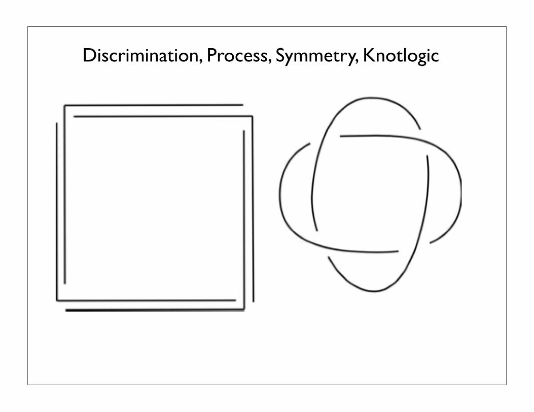
Discrimination, Process, Symmetry, Knotlogic
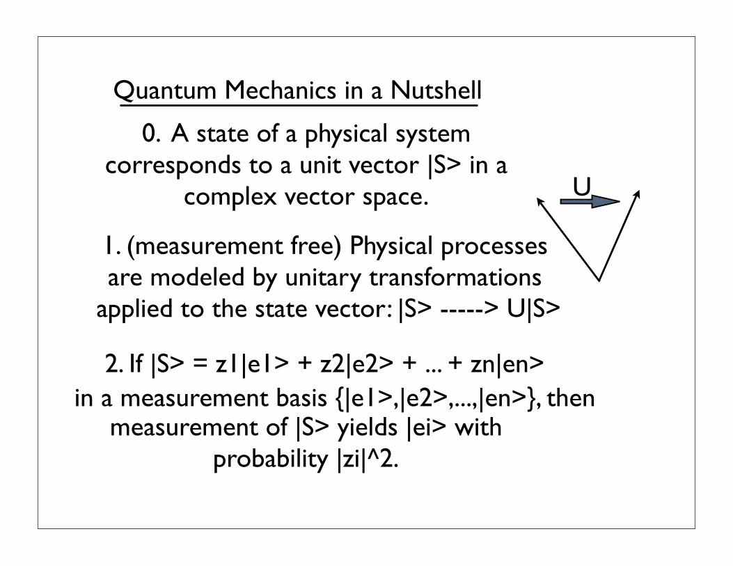
Quantum Mechanics in a Nutshell
1. (measurement free) Physical processes are modeled by unitary transformations
applied to the state vector: |S> -----> U|S>
0. A state of a physical system corresponds to a unit vector |S> in a
complex vector space.
2. If |S> = z1|e1> + z2|e2> + ... + zn|en>in a measurement basis |e1>,|e2>,...,|en>, then
measurement of |S> yields |ei> with probability |zi|^2.
U

Recalling the Diffusion Equation
x x+dxx-dx
P(x,t) = Probability that the particle is at x at time t.
P(x,t+dt) = (1/2)[P(x+dx,t) + P(x-dx,t)]
P(x,t+dt) - P(x,t) = (1/2)[P(x+dx,t) - P(x,t) -(P(x,t) - P(x-dx,t))]
,whence
dP/dt = (K/2) d P/dx2 2
K = (dx) /dt2Diffusion Equation
Diffusion Constant

Iterants
Louis H. Kauffman
Department of Mathematics, Statistics and Computer Science
University of Illinois at Chicago
851 South Morgan Street
Chicago, IL, 60607-7045
1 Introduction
The simplest discrete system corresponds directly to the square root of minus one, seen as an os-
cillation between one and minus one. This way thinking about i as an iterant is explained below.By starting with a discrete time series of positions, one has immediately a non-commutativity of
observations since the measurement of velocity involves the tick of the clock and the measur-
ment of position does not demand the tick of the clock. Commutators that arise from discrete
observation suggest a non-commutative calculus, and this calculus leads to a generalization of
standard advanced calculus in terms of a non-commutative world. In a non-commutative world,
all derivatives are represented by commutators.
Section 2 is a self-contained miniature version of the whole story in this paper, starting with
the square root of minus one seen as a discrete oscillation, a clock. We proceed from there and
analyze the position of the square root of minus one in relation to discrete systems and quantum
mechanics. We end this section by fitting together these observations into the structure of the
Heisenberg commutator
[p, q] = i!.
Section 3 is a discussion of iterants and matrix algebra. We show how matrix algebra in any
dimension can be regarded as describing the pattern of acts of observation (time shifting operators
corresponding to permutations) on periodic time series.
God Does Not Play Dice! Here is a little story about the square root of minus one and quantum
mechanics. God said - I would really like to be able to base the universe on the Diffusion Equation
∂ψ/∂t = κ∂2ψ/∂x2.
But I need to have some possibility for interference and waveforms. And it should be simple. So
I will just put a “plus or minus” ambiguity into this equation, like so:
±∂ψ/∂t = κ∂2ψ/∂x2.
An Imaginary Tale


But now with this Schroedinger equation, I should write
ψ = A + Bi
and then, since i(A + Bi) = −B + Ai, the new equation becomes two equations
∂A/∂t = κ∂2B/∂x2,
and
−∂B/∂t = κ∂2A/∂x2.
Instead of the simple diffusion equation, I have a mutual dependency where the temporal variation
ofA is mediated by the spatial variation ofB and vice-versa. This is the price I pay for not playingdice.
2 Iterants, Discrete Processes and Matrix Algebra
The primitive idea behind an iterant is a periodic time series or “waveform”
· · ·abababababab · · · .
The elements of the waveform can be any mathematically or empirically well-defined objects.
We can regard the ordered pairs [a, b] and [b, a] as abbreviations for the waveform or as two
points of view about the waveform (a first or b first). Call [a, b] an iterant. One has the collectionof transformations of the form T [a, b] = [ka, k−1b] leaving the product ab invariant. This tinymodel contains the seeds of special relativity, and the iterants contain the seeds of general matrix
algebra! For related discussion see [9, 10, 11, 12, 13, 14, 16, 28].
Define products and sums of iterants as follows
[a, b][c, d] = [ac, bd]
and
[a, b] + [c, d] = [a + c, b + d].
The operation of juxtapostion of waveforms is multiplication while + denotes ordinary addition
of ordered pairs. These operations are natural with respect to the structural juxtaposition of
iterants:
...abababababab...
...cdcdcdcdcdcd...
Structures combine at the points where they correspond. Waveforms combine at the times where
they correspond. Iterants combine in juxtaposition.
3

Question:Is there a relativistic
motivation for this binary clock
image of the Schrodinger equation?
(Compare with Garnet Ord)


Volume 4 · Number 3 · July 2009 125
concepts in second-order cyberneticsMathematical
of the world in which we operate. They attaintheir stability through the limiting processthat goes outside the immediate world ofindividual actions. We make an imaginativeleap to complete such objects to becometokens for eigenbehaviors. It is impossible tomake an infinite nest of boxes. We do notmake it. We imagine it. And in imagining thatinfinite nest of boxes, we arrive at the eigen-form.
The leap of imagination to the infiniteeigenform is a model of the human ability tocreate signs and symbols. In the case of theeigenform X with X = F(X), X can be regardedas the name of the process itself or as the nameof the limiting process. Note that if you aretold that
X = F(X),
then, substituting F(X) for X, you can write
X = F(F(X)).
Substituting again and again, you have
X = F(F(F(X))) = F(F(F(F(X)))) = F(F(F(F(F(X))))) = …
The process arises from the symbolicexpression of its eigenform. In this view, theeigenform is an implicate order for the processthat generates it. (Here we refer to implicateorder in the sense of David Bohm 1980).
Sometimes one stylizes the structure byindicating where the eigenform X reenters itsown indicational space with an arrow or othergraphical device. See the picture below for thecase of the nested boxes.
Does the infinite nest of boxes exist? Cer-tainly it does not exist on this page or any-where in the physical world with which we arefamiliar. The infinite nest of boxes exists in theimagination. It is a symbolic entity.
The eigenform is the imagined boundaryin the reciprocal relationship of the object(the “It”) and the process leading to the object(the process leading to “It”). In the diagram
below we have indicated these relationshipswith respect to the eigenform of nested boxes.Note that the “It” is illustrated as a finiteapproximation (to the infinite limit) that issufficient to allow an observer to infer/per-ceive the generating process that underlies it.
Just so, an object in the world (cognitive,physical, ideal, etc.) provides a conceptualcenter for the exploration of a skein of rela-tionships related to its context and to theprocesses that generate it. An object can havevarying degrees of reality, just as an eigenformdoes. If we take the suggestion to heart thatobjects are tokens for eigenbehaviors, then anobject in itself is an entity, participating in anetwork of interactions, taking on its appar-ent solidity and stability from theseinteractions.
An object is an amphibian between thesymbolic and imaginary world of the mindand the complex world of personal experi-ence. The object, when viewed as a process, isa dialogue between these worlds. The object,when seen as a sign for itself, or in and of itself,is imaginary.
Why are objects apparently solid? Ofcourse you cannot walk through a brick walleven if you think about it differently. I do notmean apparent in the sense of thought alone.I mean apparent in the sense of appearance.The wall appears solid to me because of the
actions that I can perform. The wall is quitetransparent to a neutrino, and will not even bean eigenform for that neutrino.
This example shows quite sharply how thenature of an object is entailed in the proper-ties of its observer.
The eigenform model can be expressed inquite abstract and general terms. Supposethat we are given a recursion (not necessarilynumerical) with the equation
X(t + 1) = F(X(t)).
Here X(t) denotes the condition of obser-vation at time t. X(t) could be as simple as aset of nested boxes, or as complex as the entireconfiguration of your body in relation to theknown universe at time t. Then F(X(t))denotes the result of applying the operationssymbolized by F to the condition at time t. Youcould, for simplicity, assume that F is inde-pendent of time. Time independence of therecursion F will give us simple answers and wecan later discuss what will happen if theactions depend upon the time. In the time-independent case we can write
J = F(F(F(…)))
– the infinite concatenation of F upon itself.Then
F(J) = J
since adding one more F to the concatenationchanges nothing.
Thus J, the infinite concatenation of theoperation upon itself leads to a fixed point forF. J is said to be the eigenform for the recur-sion F. We see that every recursion has aneigenform. Every recursion has an (imagi-nary) fixed point.
We end this section with one more exam-ple. This is the eigenform of the Koch fractal(Mandelbrot 1982). In this case one can writesymbolically the eigenform equation
K = K K K K
to indicate that the Koch Fractal reenters itsown indicational space four times (that is, it ismade up of four copies of itself, each one-third the size of the original. The curly brack-ets in the center of this equation refer to thefact that the two middle copies within thefractal are inclined with respect to oneanother and with respect to the two outercopies. In the figure below we show the geo-metric configuration of the reentry.
… =
The It
The Process leading to It... +1, -1, +1, -1, +1, -1, ...
[-1,+1] [+1,-1]
ii = -1i = -1/i
The square rootof minus one
“is”a discrete oscillation.
i as an imaginary value, defined in terms of itself.
THE SQUARE ROOT OF MINUS ONE IS A CLOCK.
From G = G to i = -1/i.

... +1, -1, +1, -1, +1, -1, +1, -1, ...
[-1,+1] [+1,-1]
Figure 29:
The square root of minus one is a perfect example of an eigenform that occurs in a new and wider
domain than the original context in which its recursive process arose. The process has no fixed
point in the original domain.
Looking at the oscillation between +1 and −1, we see that there are naturally two phase-shifted viewpoints. We denote these two views of the oscillation by [+1,−1] and[−1,+1]. Theseviewpoints correspond to whether one regards the oscillation at time zero as starting with +1 orwith −1. See Figure 29. We shall let the word iterant stand for an undisclosed alternation orambiguity between +1 and −1. There are two iterant views: [+1,−1] and [−1,+1] for the basicprocess we are examining. Given an iterant [a, b], we can think of [b, a] as the same process witha shift of one time step. The two iterant views, [+1,−1] and [−1,+1], will become the squareroots of negative unity, i and −i.
We introduce a temporal shift operator η such that
[a, b]η = η[b, a]
and
ηη = 1
for any iterant [a, b], so that concatenated observations can include a time step of one-half periodof the process
· · · abababab · · · .
We combine iterant views term-by-term as in
[a, b][c, d] = [ac, bd].
We now define i by the equation
i = [1,−1]η.
This makes i both a value and an operator that takes into account a step in time.
We calculate
ii = [1,−1]η[1,−1]η = [1,−1][−1, 1]ηη = [−1,−1] = −1.
35

and
ηη = 1
for any iterant [a, b], so that concatenated observations can include a time step of one-half periodof the process
· · ·abababab · · · .
We combine iterant views term-by-term as in
[a, b][c, d] = [ac, bd].
We now define i by the equation
i = [1,−1]η.
This makes i both a value and an operator that takes into account a step in time.
We calculate
ii = [1,−1]η[1,−1]η = [1,−1][−1, 1]ηη = [−1,−1] = −1.
Thus we have constructed a square root of minus one by using an iterant viewpoint. In this view
i represents a discrete oscillating temporal process and it is an eigenform for T (x) = −1/x,participating in the algebraic structure of the complex numbers. In fact the corresponding algebra
structure of linear combinations [a, b]+[c, d]η is isomorphic with 2×2matrix algebra and iterantscan be used to construct n × n matrix algebra. We treat this generalization elsewhere [72, 73].
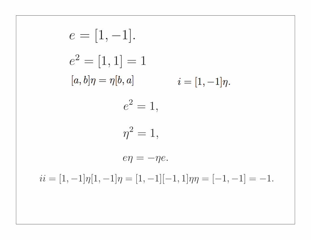
Now we can make contact with the algebra of the Majorana fermions. Let e = [1,−1]. Thenwe have e2 = [1, 1] = 1 and eη = [1,−1]η = [−1, 1]η = −eη. Thus we have
e2 = 1,
η2 = 1,
and
eη = −ηe.
We can regard e and η as a fundamental pair of Majorana fermions. This is a formal corre-spondence, but it is striking how this Marjorana fermion algebra emerges from an analysis of
the recursive nature of the reentering mark, while the fusion algebra for the Majorana fermion
emerges from the distinctive properties of the mark itself. We see how the seeds of the fermion
algebra live in this extended logical context.
Note how the development of the algebra works at this point. We have that
(eη)2 = −1
and so regard this as a natural construction of the square root of minus one in terms of the phase
synchronization of the clock that is the iteration of the reentering mark. Once we have the square
36
and
ηη = 1
for any iterant [a, b], so that concatenated observations can include a time step of one-half periodof the process
· · ·abababab · · · .
We combine iterant views term-by-term as in
[a, b][c, d] = [ac, bd].
We now define i by the equation
i = [1,−1]η.
This makes i both a value and an operator that takes into account a step in time.
We calculate
ii = [1,−1]η[1,−1]η = [1,−1][−1, 1]ηη = [−1,−1] = −1.
Thus we have constructed a square root of minus one by using an iterant viewpoint. In this view
i represents a discrete oscillating temporal process and it is an eigenform for T (x) = −1/x,participating in the algebraic structure of the complex numbers. In fact the corresponding algebra
structure of linear combinations [a, b]+[c, d]η is isomorphic with 2×2matrix algebra and iterantscan be used to construct n × n matrix algebra. We treat this generalization elsewhere [72, 73].
Now we can make contact with the algebra of the Majorana fermions. Let e = [1,−1]. Thenwe have e2 = [1, 1] = 1 and eη = [1,−1]η = [−1, 1]η = −eη. Thus we have
e2 = 1,
η2 = 1,
and
eη = −ηe.
We can regard e and η as a fundamental pair of Majorana fermions. This is a formal corre-spondence, but it is striking how this Marjorana fermion algebra emerges from an analysis of
the recursive nature of the reentering mark, while the fusion algebra for the Majorana fermion
emerges from the distinctive properties of the mark itself. We see how the seeds of the fermion
algebra live in this extended logical context.
Note how the development of the algebra works at this point. We have that
(eη)2 = −1
and so regard this as a natural construction of the square root of minus one in terms of the phase
synchronization of the clock that is the iteration of the reentering mark. Once we have the square
36

[a,b] + [c,d]!
and it is not hard to see that this is isomorphic with 2 x 2 matrix algebra with the correspondence given by the diagram below.
[a,b] + [c,d] a c
d b!
Figure 23 We see from this excursion that there is a full interpretation for the complex numbers (and indeed matrix algebra) as an observational system taking into account time shifts for underlying iterant processes. Let A = [a,b] and B = [c,d] and let C = [r,s], D = [t,u]. With A' = [b,a], we have
(A + B!)(C+D!) = (AC + BD') + (AD + BC')! .
This writes 2 x 2 matrix algebra in the form of a hypercomplex number system. From the point of view of iterants, the sum [a,b] + [b,c]! can be regarded as a superposition of two types of
observation of the iterants Ia,b and Ic,d. The operator-view [c,d]! includes the shift that will move the viewpoint from
[c,d] to [d,c], while [a,b] does not contain this shift. Thus a shift of viewpoint on [c,d] in this superposition does not affect the values of [a,b]. One can think of the corresponding process as having the form shown below.
... a a a a a a a a a a a a a a a ... ... c d c d c d c d c d c d c d ...
... b b b b b b b b b b b b b b ... The snapshot [c,d] changes to [d,c] in the horizontal time-shift while the vertical snapshot [a,b] remains invariant under the shift. It is interesting to note that in the spatial explication of the process we can imagine the horizontal oscillation corresponding to [c,d]!
as making a boundary (like a frieze pattern), while the vertical iterant parts a and b mark the two sides of that boundary.
root of minus one it is natural to introduce another one and call this one i, letting it commute withthe other operators. Then we have the (ieη)2 = +1 and so we have a triple of Majorana fermions:
a = e, b = η, c = ieη
and we can construct the quaternions
I = ba = ηe, J = cb = ie, K = ac = iη.
With the quaternions in place, we have the braiding operators
A =1√2(1 + I), B =
1√2(1 + J), C =
1√2(1 + K),
and can continue as we did in Section 4.
There is one more comment that is appropriate for this section. Recall from Section 4 that a
pair of Majorana fermions can be assembled to form a single standard fermion. In our case we
have the two Marjorana fermions e and η and the corresponding standard fermion annihilationand creation operators are then given by the formulas below.
ψ = (e + iη)/2
and
ψ† = (e − iη)/2.
Since e represents a spatial view of the basic discrete oscillation and η is the time-shift operatorfor this oscillation it is of interest to note that the standard fermion built by these two can be
regarded as a quantum of spacetime, retrieved from the way that we decomposed the process into
space and time. Since all this is initially built in relation to extending the Boolean logic of the
mark to a non-boolean recursive context, there is further analysis needed of the relation of the
physics and the logic. This will be taken up in a separate paper.
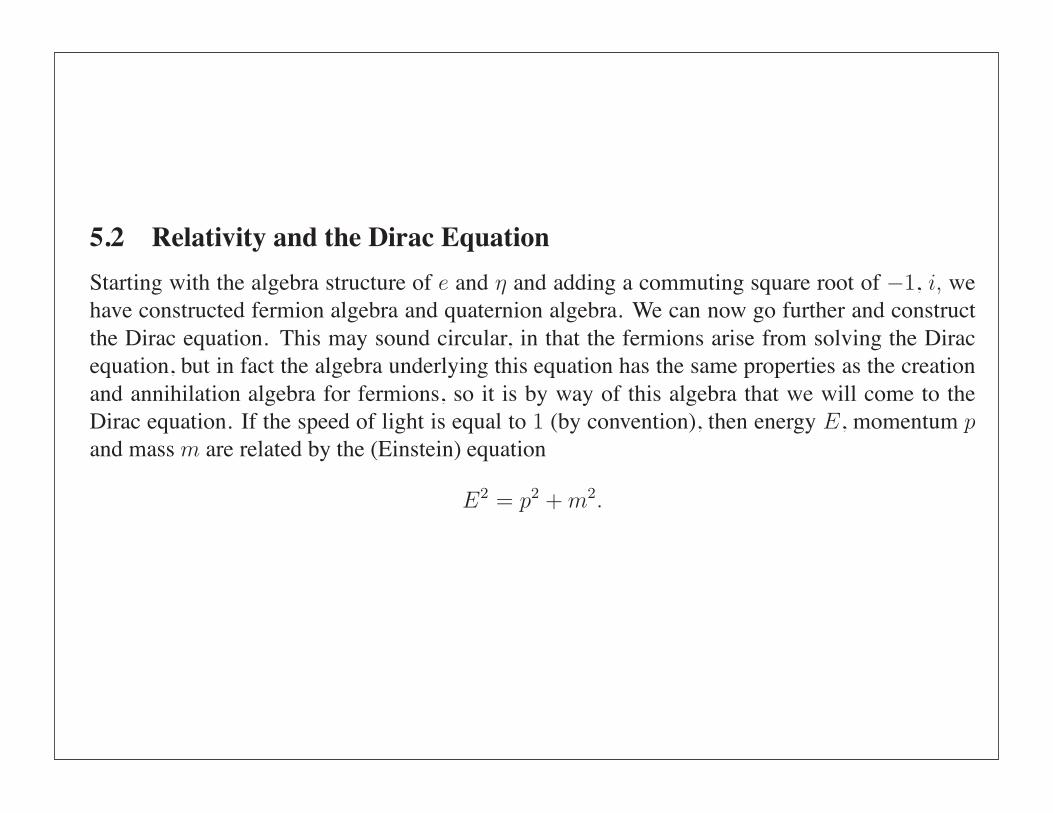
5.2 Relativity and the Dirac Equation
Starting with the algebra structure of e and η and adding a commuting square root of −1, i, wehave constructed fermion algebra and quaternion algebra. We can now go further and construct
the Dirac equation. This may sound circular, in that the fermions arise from solving the Dirac
equation, but in fact the algebra underlying this equation has the same properties as the creation
and annihilation algebra for fermions, so it is by way of this algebra that we will come to the
Dirac equation. If the speed of light is equal to 1 (by convention), then energy E, momentum pand massm are related by the (Einstein) equation
E2 = p2 + m2.
37
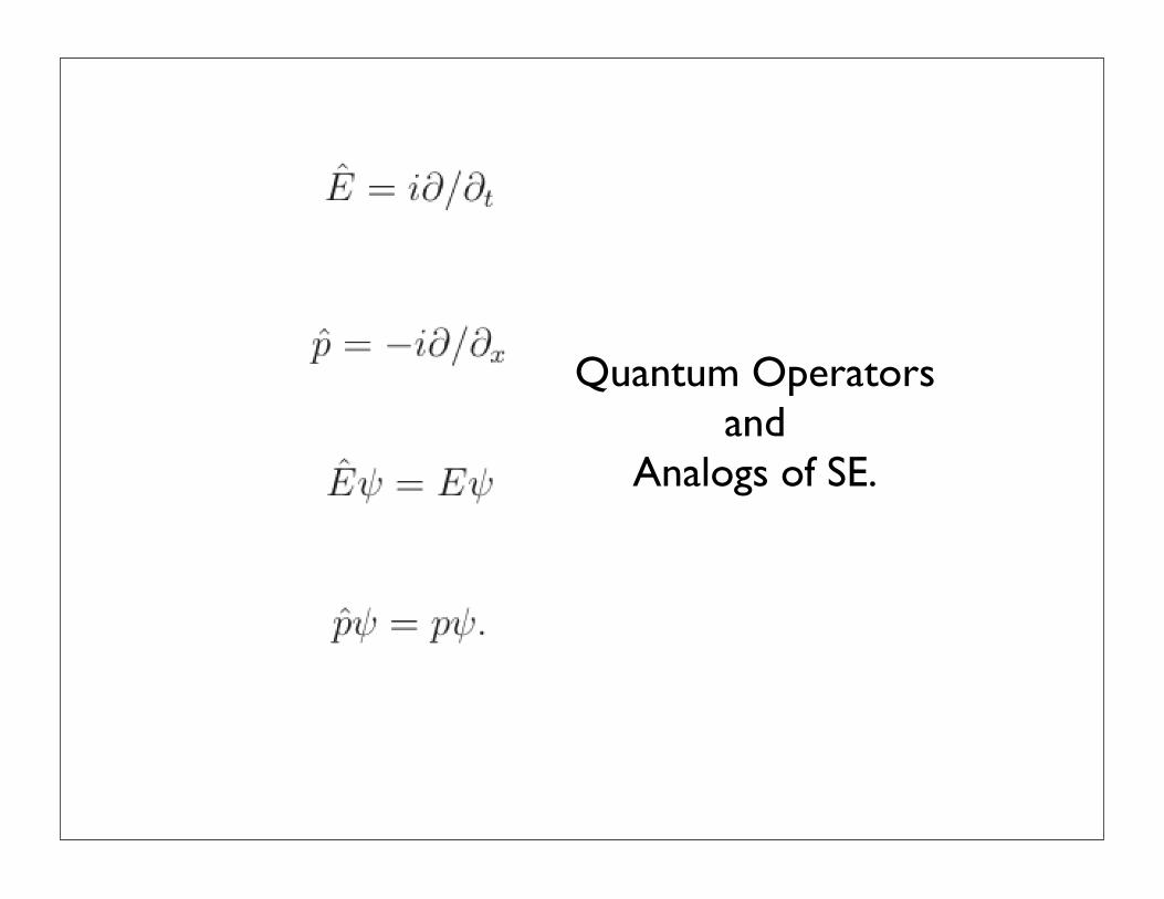
Quantum Operatorsand
Analogs of SE.
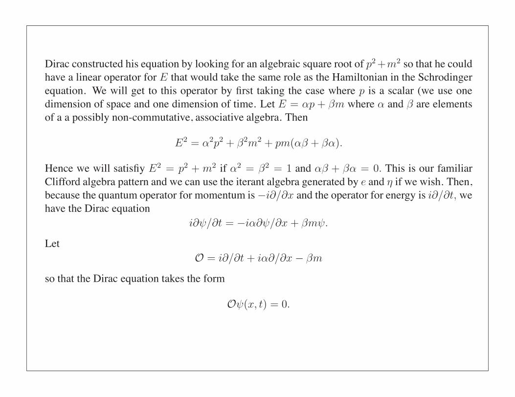
Dirac constructed his equation by looking for an algebraic square root of p2 +m2 so that he could
have a linear operator for E that would take the same role as the Hamiltonian in the Schrodinger
equation. We will get to this operator by first taking the case where p is a scalar (we use onedimension of space and one dimension of time. Let E = αp + βm where α and β are elementsof a a possibly non-commutative, associative algebra. Then
E2 = α2p2 + β2m2 + pm(αβ + βα).
Hence we will satisfiy E2 = p2 + m2 if α2 = β2 = 1 and αβ + βα = 0. This is our familiarClifford algebra pattern and we can use the iterant algebra generated by e and η if we wish. Then,because the quantum operator for momentum is−i∂/∂x and the operator for energy is i∂/∂t, wehave the Dirac equation
i∂ψ/∂t = −iα∂ψ/∂x + βmψ.
Let
O = i∂/∂t + iα∂/∂x − βm
so that the Dirac equation takes the form
Oψ(x, t) = 0.
Now note that
Oei(px−Et) = (E − αp + βm)ei(px−Et)
and that if
U = (E − αp + βm)βα = βαE + βp + αm,
then
U2 = −E2 + p2 + m2 = 0,
from which it follows that
ψ = Uei(px−Et)
is a (plane wave) solution to the Dirac equation.
In fact, this calculation suggests that we should multiply the operator O by βα on the right,obtaining the operator
D = Oβα = iβα∂/∂t + iβ∂/∂x + αm,
and the equivalent Dirac equation
Dψ = 0.
In fact for the specific ψ above we will now have D(Uei(px−Et)) = U2ei(px−Et) = 0. This wayof reconfiguring the Dirac equation in relation to nilpotent algebra elements U is due to Peter
Rowlands [94]. We will explore this relationship with the Rowlands formulation in a separate
paper.
38

9.1 Another version of U and U †
We start with ψ = ei(px−Et) and the operators
E = i∂/∂t
and
p = −i∂/∂x
so that
Eψ = Eψ
and
pψ = pψ.
The Dirac operator is
O = E − αp − βm
and the modified Dirac operator is
D = Oβα = βαE + βp − αm,
so that
Dψ = (βαE + βp − αm)ψ = Uψ.
If we let
ψ = ei(px+Et)
(reversing time), then we have
Dψ = (−βαE + βp − αm)ψ = U †ψ,
giving a definition of U † corresponding to the anti-particle for Uψ.
We have that
U2 = U †2 = 0
and
UU † + U †U = 4E2.
Thus we have a direct appearance of the Fermion algebra corresponding to the Fermion plane
wave solutions to the Dirac equation.
38
This is a route to Peter Rowland’s Nilpotent operators.


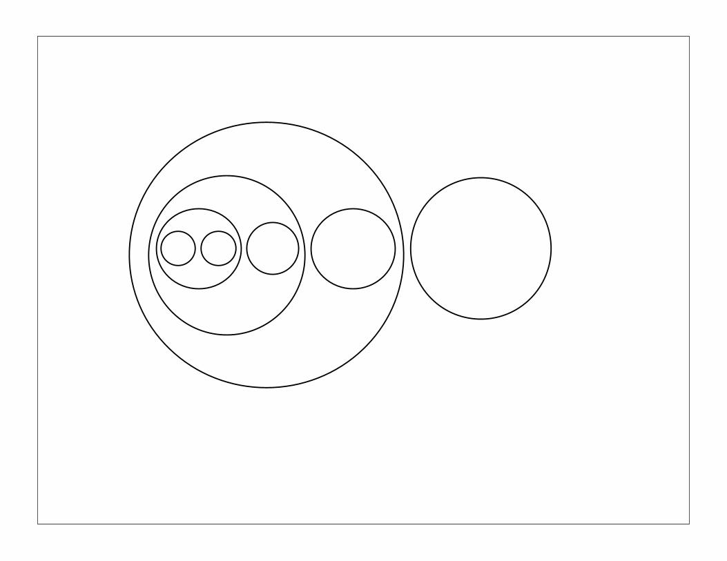
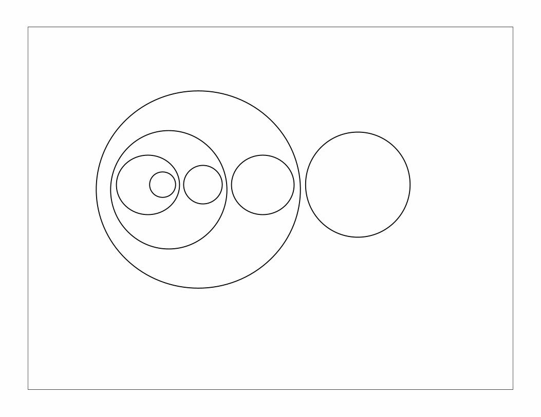
Fibonacci Process
P P
P
P P
*
The “particle” P interacts with Pto produce either P or *.The particle * is neutral.

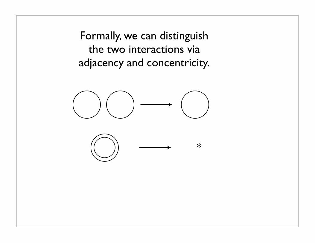
Formally, we can distinguish the two interactions via
adjacency and concentricity.
*
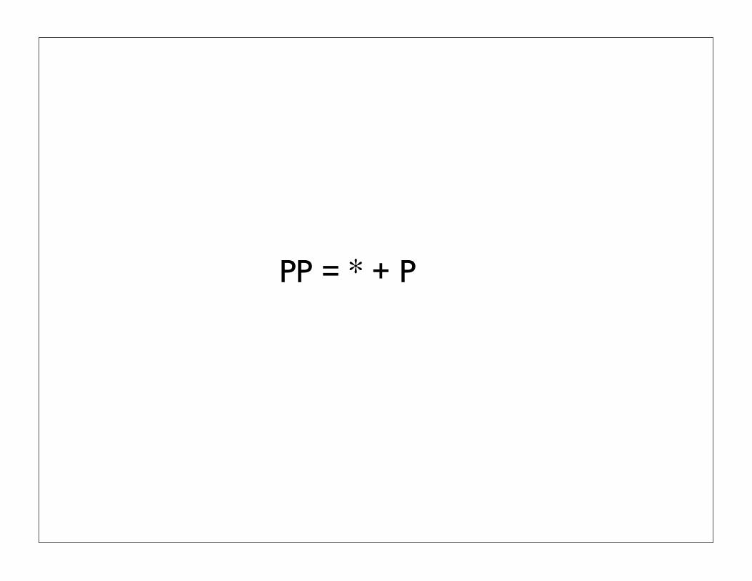
PP = * + P
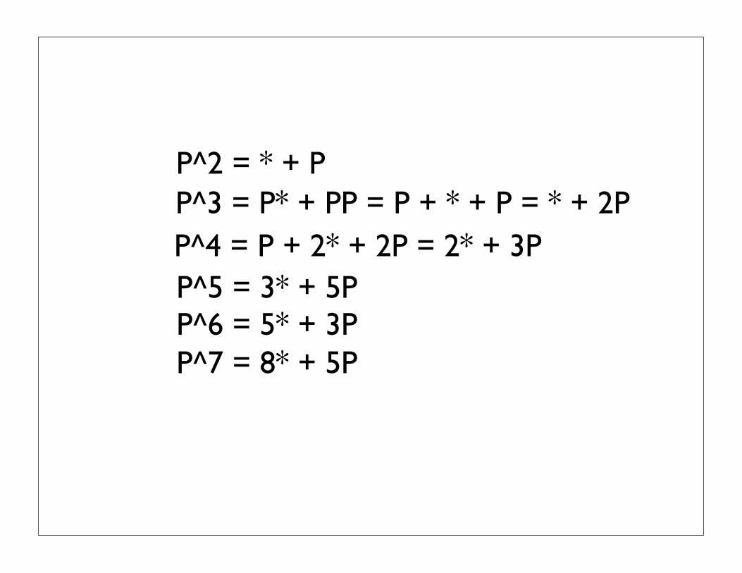
P^2 = * + PP^3 = P* + PP = P + * + P = * + 2P P^4 = P + 2* + 2P = 2* + 3P
P^5 = 3* + 5P P^6 = 5* + 3P P^7 = 8* + 5P
P P P P P P
P
P
*
P
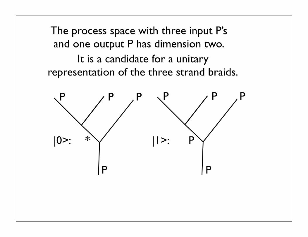
|1>:|0>:
The process space with three input P’s and one output P has dimension two.
It is a candidate for a unitary representation of the three strand braids.

Fibonacci Tree of Particle Interactions

Fibonacci Tree:
Admissible Sequencesare the Paths from the Root

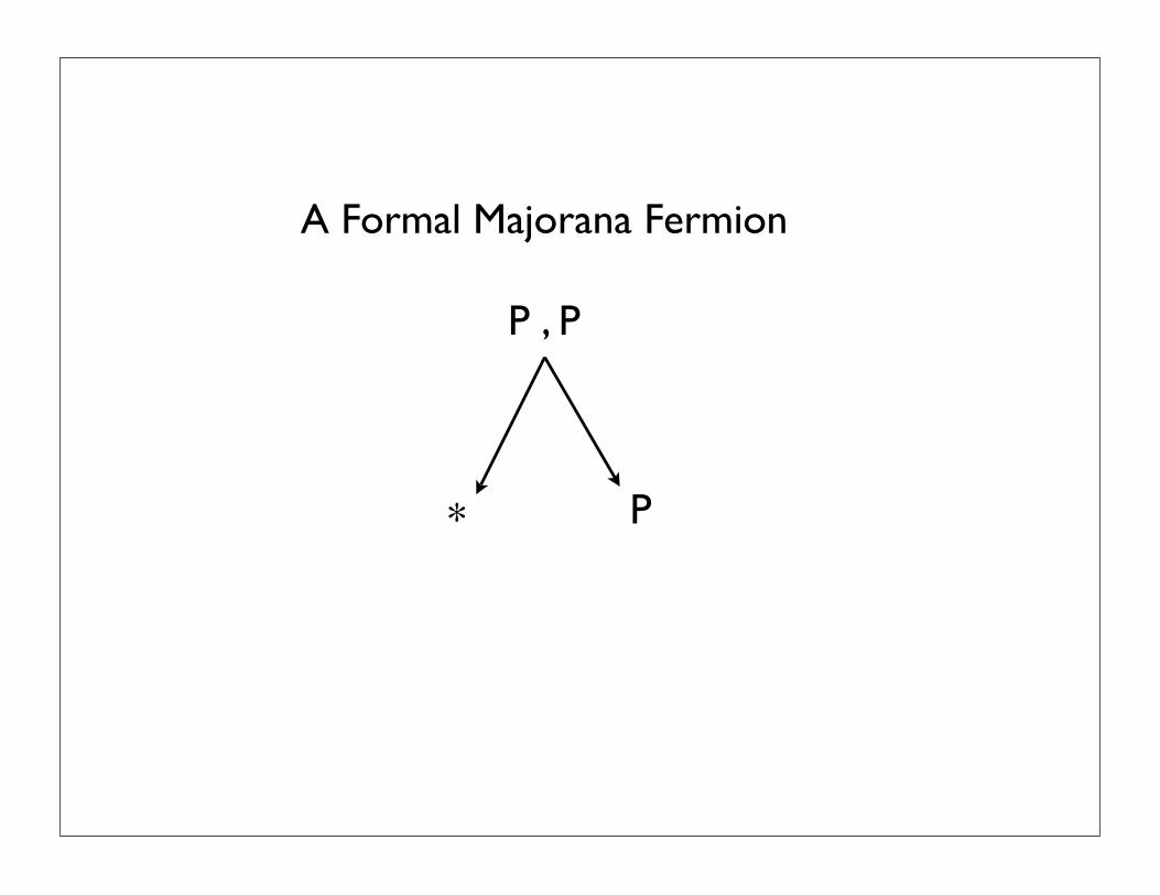
P , P
* P
A Formal Majorana Fermion

The Creation/Annihilation algebra for a Majorana Fermion is very simple.
Just an element a with aa =1. If there are two Majorana Fermions, we have
a,bwith aa = 1, bb=1 and
ab +ba = 0.
An Elementary Particle has a Fusion Algebra and a Creation/Annihilation Algebra.

For a standard Fermion there is a an annihilation operator F
and a creation operator F*.
These correspond to the fact thatthe antiparticle is distinct from the
particle.
We have FF = F*F* =0but
FF* + F*F = 1.

Mathematically an Electron’s creation and annihilation operators are
combinations of Majorana Fermion operators: U = a + ib and U* = a - ib
where ab+ba = 0 and aa =bb=1.
Majorana Fermions are their own antiparticles.
Are electrons composites of pairs
of Majorana fermions?
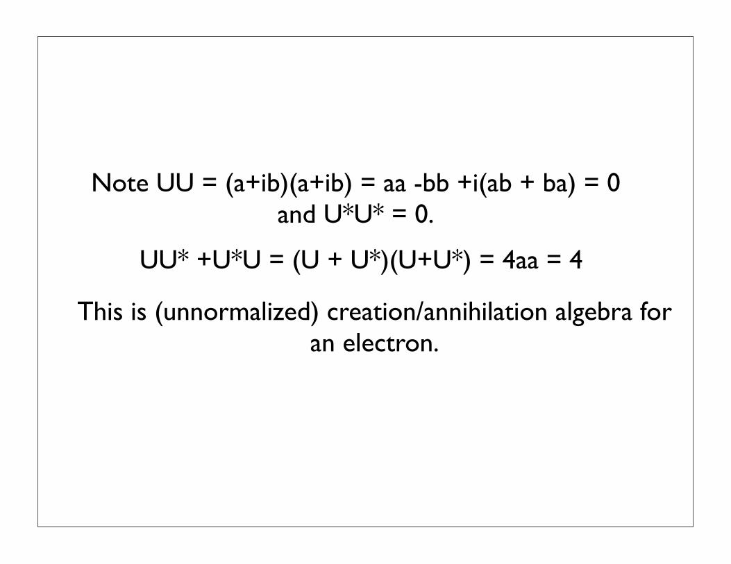
Note UU = (a+ib)(a+ib) = aa -bb +i(ab + ba) = 0and U*U* = 0.
UU* +U*U = (U + U*)(U+U*) = 4aa = 4
This is (unnormalized) creation/annihilation algebra for an electron.

A possible sighting of Majorana statesNearly 80 years ago, the Italian physicist Ettore Majorana proposed the existence of an unusual type of particle that is its own antiparticle, the so-called Majorana fermion. The search for a free Majorana fermion has so far been unsuccessful, but bound Majorana-like collective excitations may exist in certain exotic superconductors. Nadj-Perge et al. created such a topological superconductor by depositing iron atoms onto the surface of superconducting lead, forming atomic chains (see the Perspective by Lee). They then used a scanning tunneling microscope to observe enhanced conductance at the ends of these chains at zero energy, where theory predicts Majorana states should appear.

arX
iv:c
on
d-m
at/
00
10
44
0v
2
[co
nd
-mat.
mes-
hall
] 3
0 O
ct
20
00
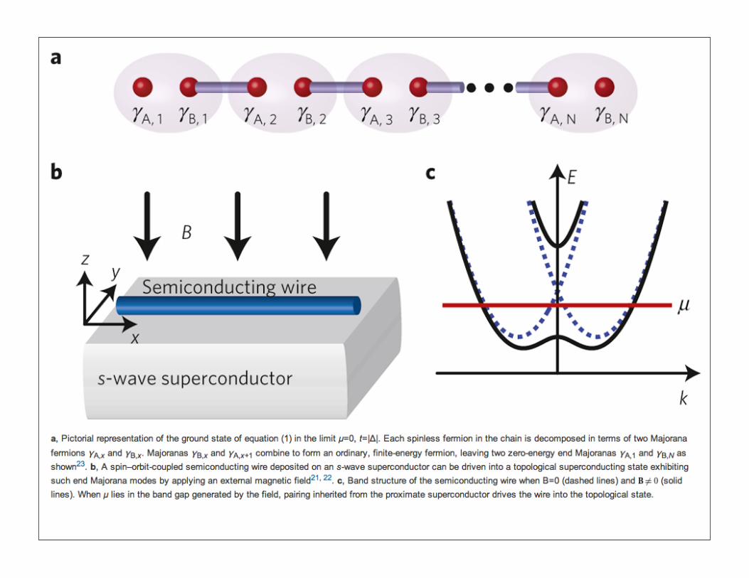
Unpaired Majorana fermions in quantum wires
Alexei Yu. Kitaev∗
Microsoft ResearchMicrosoft, #113/2032, One Microsoft Way,
Redmond, WA 98052, [email protected]
27 October 2000
Abstract
Certain one-dimensional Fermi systems have an energy gap in thebulk spectrum while boundary states are described by one Majoranaoperator per boundary point. A finite system of length L possesses twoground states with an energy difference proportional to exp(−L/l0)and different fermionic parities. Such systems can be used as qubitssince they are intrinsically immune to decoherence. The property of asystem to have boundary Majorana fermions is expressed as a condi-tion on the bulk electron spectrum. The condition is satisfied in thepresence of an arbitrary small energy gap induced by proximity of a3-dimensional p-wave superconductor, provided that the normal spec-trum has an odd number of Fermi points in each half of the Brillouinzone (each spin component counts separately).
Introduction
Implementing a full scale quantum computer is a major challenge to mod-ern physics and engineering. Theoretically, this goal should be achievable
∗On leave from L. D. Landau Institute for Theoretical Physics
1
In terms of this operators, the Hamiltonian becomes
H1 =i
2
!
j
"
−µc2j−1c2j + (w + |∆|)c2jc2j+1 + (−w + |∆|)c2j−1c2j+2
#
. (6)
Let us start with two special cases.
a) The trivial case: |∆| = w = 0, µ < 0. Then H1 = −µ$
j(a†jaj −
12) =
i2(−µ)
$
j c2j−1c2j . The Majorana operators c2j−1, c2j from the samesite j are paired together to form a ground state with the occupationnumber 0.
b) |∆| = w > 0, µ = 0. In this case
H1 = iw!
j
c2jc2j+1. (7)
Now the Majorana operators c2j , c2j+1 from different sites are pairedtogether (see fig. 2). One can define new annihilation and creationoperators aj = 1
2(c2j + ic2j+1), a†j = 1
2(c2j − ic2j+1) which span the sites
j and j + 1. The Hamiltonian becomes 2w$L−1
j=1 (a†jaj −
12). Ground
states satisfy the condition aj |ψ⟩ = 0 for j = 1, . . . , L − 1. There aretwo orthogonal states |ψ0⟩ and |ψ1⟩ with this property. Indeed, theMajorana operators b′ = c1 and b′′ = c2L remain unpaired (i. e. do notenter the Hamiltonian), so we can write
− ib′b′′|ψ0⟩ = |ψ0⟩, −ib′b′′|ψ1⟩ = −|ψ1⟩. (8)
% %c1 c2
% %c3 c4
. . .
% %c2L−1 c2L
a)
% %c1 c2
% %c3 c4
. . .
% %c2L−1 c2L
b)
Figure 2: Two types of pairing.
Note that the state |ψ0⟩ has an even fermionic parity (i. e. it is a superpositionof states with even number of electrons) while |ψ1⟩ has an odd parity. Theparity is measured by the operator
P =%
j
(−ic2j−1c2j). (9)
5
arX
iv:c
on
d-m
at/0
00
50
69
v2
[c
on
d-m
at.s
up
r-co
n]
11
May
20
00
Non-abelian statistics of half-quantum vortices in p-wave superconductors
D. A. IvanovInstitut fur Theoretische Physik, ETH-Honggerberg, CH-8093 Zurich, Switzerland
(May 11, 2000)
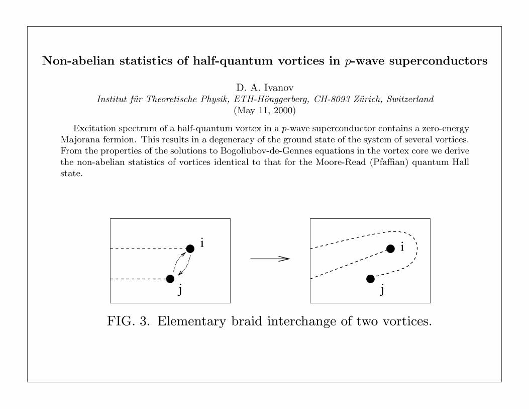
Excitation spectrum of a half-quantum vortex in a p-wave superconductor contains a zero-energyMajorana fermion. This results in a degeneracy of the ground state of the system of several vortices.From the properties of the solutions to Bogoliubov-de-Gennes equations in the vortex core we derivethe non-abelian statistics of vortices identical to that for the Moore-Read (Pfaffian) quantum Hallstate.
Certain types of superconductors with triplet pairing allow half-quantum vortices [1]. Such vortices appear if themulti-component order parameter has extra degrees of freedom besides the overall phase, and the vortex involvesboth a rotation of the phase by π and a rotation of the “direction” of the order parameter by π, so that the orderparameter maps to itself on going around the vortex. The magnetic flux through such a vortex is one half of thesuperconducting flux quantum Φ0.
Another signature of this unusual flux quantization is a Majorana fermion level at zero energy inside the vortexcore [2]. This energy level has a topological nature [3] and from the continuity considerations must be stable to anylocal perturbations. In terms of the energy levels, the Majorana fermions in vortex cores imply a 2n-fold degeneracyof the ground state of a system with 2n isolated vortices. If we let vortices adiabatically move around each other,this motion may result in a unitary transformation in the space of ground states (non-abelian statistics). We shallsee that it is indeed the case.
The non-abelian statistics for half-quantum vortices has been originally derived for the Pfaffian quantum Hallstate proposed by Moore and Read [4]. The Pfaffian state is of Laughlin type and may be possibly realized forfilling fractions with even denominator. The excitations in the Pfaffian state are half-quantum vortices, and theirnon-abelian statistics has been derived in the field-theoretical framework [5–8].
On the other hand, recently Read and Green suggested that the Pfaffian state belongs to the same topological classas the BCS pairing state and thus the latter must have the same non-abelian statistics [2]. In our paper we verifythis directly in the BCS framework as the property of solutions to Bogoliubov-de-Gennes equations. Our derivationprovides an alternative (and possibly more transparent) point of view on the non-abelian statistics of half-quantumvortices as well as an additional verification of topological equivalence between Pfaffian and BCS states.
Let us begin our discussion with reviewing the properties of a half-quantum vortex. To be specific, we considera chiral two-dimensional superconductor with the order parameter of A phase of 3He. The order parameter ischaracterized by the direction d of the spin triplet (the projection on which of the spin of the Cooper pair is zero)and by the overall phase ϕ. The wave function of the condensate is
Ψ± = eiϕ
!
dx
"
|↑↑⟩ + |↓↓⟩#
+ idy
"
|↑↑⟩ − |↓↓⟩#
+ dz
"
|↑↓⟩ + |↓↑⟩#
$
(kx ± iky). (1)
The ± signs denote the two possible chiralities of the condensate. The chirality breaks the time-reversal symmetryand means a non-zero angular momentum of the Cooper pairs. In a physical chiral superconductor there must existdomain walls separating domains of opposite chirality. Experimentally, domain walls may possibly be expelled fromthe sample by an external field which makes one of the chiralities energetically favorable. In our discussion we do notconsider interaction of vortices with domain walls, but assume that the chirality is fixed over the region where thevortex braiding occurs (and takes positive sign in eq.(1)).
For the half-quantum vortex to exist, the vector d must be able to rotate (either in a plane or in all three dimensions).An important observation is that the order parameter maps to itself under simultaneous change of sign of the vectord and shift of the phase ϕ by π: (ϕ, d) %→ (ϕ + π,−d). The half-quantum vortex then combines rotations of thevector d by π and of the phase ϕ by π on going around the vortex core (Fig. 1). This vortex is topologically stable,i.e. it cannot be removed by a continuous (homotopic) deformation of the order parameter.
Without loss of generality, we consider the vector d rotating in the x-y plane. The direction of the rotation of thephase ϕ may either coincide or be opposite to the chirality of the condensate, which defines either a positive (Φ = 1/2)or a negative (Φ = −1/2) vortex respectively.
There are also two possible directions of rotating the vector d. If the vector d is confined to a plane (i.e. takesvalues on a one-dimensional circle) by an anisotropy interaction, this gives two possible winding numbers of the vector
1
Ti :
⎧
⎨
⎩
ci !→ ci+1
ci+1 !→ −ci
cj !→ cj for j = i and j = i + 1(8)
This defines the action of Ti on Majorana fermions. One easily checks that this action obeys the commutation relations(7).
i
j
i
j
FIG. 3. Elementary braid interchange of two vortices.
Now the action of operators Ti may be extended from operators to the Hilbert space. Since the whole Hilbert spacecan be constructed from the vacuum state by fermionic creation operators, and the mapping of the vacuum state byTi may be determined uniquely up to a phase factor, the action (8) of B2n on operators uniquely defines a projectiverepresentation of B2n in the space of ground states.
The explicit formulas for this representation may be written in terms of fermionic operators. Namely, we needto construct operators τ(Ti) obeying τ(Ti)cj [τ(Ti)]−1 = Ti(cj), where Ti(cj) is defined by (8). If we normalize theMajorana fermions by
ci, cj = 2δij, (9)
then the expression for τ(Ti) is
τ(Ti) = exp(π
4ci+1ci
)
=1√2
(1 + ci+1ci) (10)
(up to a phase factor).This formula presents the main result of our calculation. On inspection, this representation coincides with that
described by Nayak and Wilczek for the statistics of the Pfaffian state [5] (our Majorana fermions correspond to theoperators γi in section 9 of their paper).
The two simplest examples of the representation (10) are the cases of two and four vortices. These examples werepreviously discussed to some extent in the Pfaffian framework in refs. [5,6], and we review them here for illustrationpurposes.
In the case of two vortices, the two Majorana fermions may be combined into a single complex fermion as Ψ =(c1 + ic2)/2, Ψ† = (c1 − ic2)/2. The ground state is doubly degenerate, and the only generator of the braid group Tis represented by
τ(T ) = exp(π
4c2c1
)
= exp[
iπ
4(2Ψ†Ψ− 1)
]
= exp(
iπ
4σz
)
, (11)
where σz is a Pauli matrix in the basis (|0⟩, Ψ† |0⟩).In the case of four vortices, the four Majorana fermions combine into two complex fermions Ψ1 and Ψ2 by Ψ1 =
(c1 + ic2)/2, Ψ2 = (c3 + ic4)/2 (and similarly for Ψ†1 and Ψ†
2). The ground state has degeneracy four, and the threegenerators T1, T2, and T3 of the braid group are represented by
τ(T1) = exp(
iπ
4σ(1)
z
)
=
⎛
⎜
⎝
e−iπ/4
eiπ/4
e−iπ/4
eiπ/4
⎞
⎟
⎠,
τ(T3) = exp(
iπ
4σ(2)
z
)
=
⎛
⎜
⎝
e−iπ/4
e−iπ/4
eiπ/4
eiπ/4
⎞
⎟
⎠, (12)
τ(T2) = exp(π
4c3c2
)
=1√2(1 + c3c2) =
1√2
[
1 + i(Ψ†2 + Ψ2)(Ψ
†1 −Ψ1)
]
=1√2
⎛
⎜
⎝
1 0 0 −i0 1 −i 00 −i 1 0−i 0 0 1
⎞
⎟
⎠,
4

Evidence for Majorana fermions in a nanowireR. Mark Wilson
June 2012, page 14DIGITAL OBJECT IDENTIFIERhttp://dx.doi.org/10.1063/PT.3.1587Electrical conductance measurements reveal what may be massless, chargeless, and spinless quasiparticles of zero energy.
Physics Today

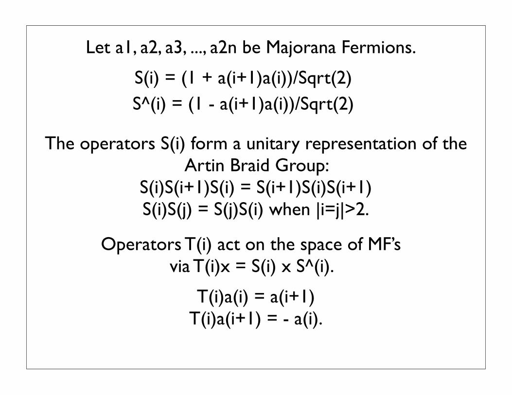
Let a1, a2, a3, ..., a2n be Majorana Fermions.
S(i) = (1 + a(i+1)a(i))/Sqrt(2)
Operators T(i) act on the space of MF’svia T(i)x = S(i) x S^(i).
S^(i) = (1 - a(i+1)a(i))/Sqrt(2)
T(i)a(i) = a(i+1)T(i)a(i+1) = - a(i).
The operators S(i) form a unitary representation of the Artin Braid Group:
S(i)S(i+1)S(i) = S(i+1)S(i)S(i+1)S(i)S(j) = S(j)S(i) when |i=j|>2.

8 Clifford Algebra, Majorana Fermions and Braiding
Recall fermion algebra. One has fermion annihiliation operators ψ and their conjugate creationoperators ψ†. One has ψ2 = 0 = (ψ†)2. There is a fundamental commutation relation
ψψ† + ψ†ψ = 1.
If you have more than one of them say ψ and φ, then they anti-commute:
ψφ = −φψ.
The Majorana fermions c that satisfy c† = c so that they are their own anti-particles. There is a lotof interest in these as quasi-particles and they are related to braiding and to topological quantum
computing. A group of researchers [?] claims, at this writing, to have found quasiparticle Majo-
rana fermions in edge effects in nano-wires. (A line of fermions could have a Majorana fermion
happen non-locally from one end of the line to the other.) The Fibonacci model that we discuss is
also based on Majorana particles, possibly related to collecctive electronic excitations. If P is a
Majorana fermion particle, then P can interact with itself to either produce itself or to annihilate
itself. This is the simple “fusion algebra” for this particle. One can write P 2 = P + 1 to denotethe two possible self-interactions the particle P. The patterns of interaction and braiding of sucha particle P give rise to the Fibonacci model.
Majoranas are related to standard fermions as follows: The algebra for Majoranas is c = c†
and cc′ = −c′c if c and c′ are distinct Majorana fermions with c2 = 1 and c′2 = 1. One can makea standard fermion from two Majoranas via
ψ = (c + ic′)/2,
ψ† = (c − ic′)/2.
Similarly one can mathematically make two Majoranas from any single fermion. Now if you take
a set of Majoranas
c1, c2, c3, · · · , cn
then there are natural braiding operators that act on the vector space with these ck as the basis.
The operators are mediated by algebra elements
τk = (1 + ck+1ck)/√
2,
τ−1k = (1 − ck+1ck)/
√2.
Then the braiding operators are
Tk : Spanc1, c2, · · · , , cn −→ Spanc1, c2, · · · , , cn
via
Tk(x) = τkxτ−1k .
30

It is worth noting that a triple of Majorana fermions say a, b, c gives rise to a representationof the quaternion group. This is a generalization of the well-known association of Pauli matrices
and quaternions. We have a2 = b2 = c2 = 1 and they anticommute. Let I = ba, J = cb, K = ac.Then
I2 = J2 = K2 = IJK = −1,
giving the quaternions. The operators
A = (1/√
2)(1 + I)
B = (1/√
2)(1 + J)
C = (1/√
2)(1 + K)
braid one another:
ABA = BAB, BCB = CBC, ACA = CAC.
This is a special case of the braid group representation described above for an arbitrary list of
Majorana fermions. These braiding operators are entangling and so can be used for universal
quantum computation, but they give only partial topological quantum computation due to the
interaction with single qubit operators not generated by them.
In Section 5 we show how the dynamics of the reentering mark leads to two (algebraic)
Majorana fermions e and η that correspond to the spatial and temporal aspects of this recursiveprocess. The corresponding standard fermion operators are then given by the formulas below.
ψ = (e + iη)/2
and
ψ† = (e − iη)/2.
This gives a model of a fermion creation operator as a point in a non-commutative spacetime. This
suggestive point of view, based on knot logic and Laws of Form, will be explored in subsequent
publications.
Topological quantum computing. This paper describes relationships between quantum topol-
ogy and quantum computing as a modified version of Chapter 14 of the book [13] and an ex-
panded version of [67] and an expanded version of a chapter in [81]. Quantum topology is,
roughly speaking, that part of low-dimensional topology that interacts with statistical and quan-
tum physics. Many invariants of knots, links and three dimensional manifolds have been born of
this interaction, and the form of the invariants is closely related to the form of the computation of
amplitudes in quantum mechanics. Consequently, it is fruitful to move back and forth between
quantum topological methods and the techniques of quantum information theory.
5
=
RIR I
RI
RI
RI
R I
R I
R I
Figure 30: The Yang-Baxter equation
A solution to the Yang-Baxter equation, as described in the last paragraph is a matrix R,regarded as a mapping of a two-fold tensor product of a vector space V ⊗V to itself that satisfies
the equation
(R ⊗ I)(I ⊗ R)(R ⊗ I) = (I ⊗ R)(R ⊗ I)(I ⊗ R).
From the point of view of topology, the matrix R is regarded as representing an elementary bit
of braiding represented by one string crossing over another. In Figure 30 we have illustrated
the braiding identity that corresponds to the Yang-Baxter equation. Each braiding picture with
its three input lines (below) and output lines (above) corresponds to a mapping of the three fold
tensor product of the vector space V to itself, as required by the algebraic equation quoted above.
The pattern of placement of the crossings in the diagram corresponds to the factors R ⊗ I andI ⊗ R. This crucial topological move has an algebraic expression in terms of such a matrix R.Our approach in this section to relate topology, quantum computing, and quantum entanglement
is through the use of the Yang-Baxter equation. In order to accomplish this aim, we need to study
solutions of the Yang-Baxter equation that are unitary. Then the R matrix can be seen either as a
braiding matrix or as a quantum gate in a quantum computer.
The problem of finding solutions to the Yang-Baxter equation that are unitary turns out to be
surprisingly difficult. Dye [18] has classified all such matrices of size 4 × 4. A rough summaryof her classification is that all 4 × 4 unitary solutions to the Yang-Baxter equation are similar toone of the following types of matrix:
R =
⎛
⎜
⎜
⎜
⎜
⎝
1/√
2 0 0 1/√
20 1/
√2 −1/
√2 0
0 1/√
2 1/√
2 0−1/
√2 0 0 1/
√2
⎞
⎟
⎟
⎟
⎟
⎠
R′ =
⎛
⎜
⎜
⎜
⎝
a 0 0 00 0 b 00 c 0 00 0 0 d
⎞
⎟
⎟
⎟
⎠
43
ABA
BAB
-
+
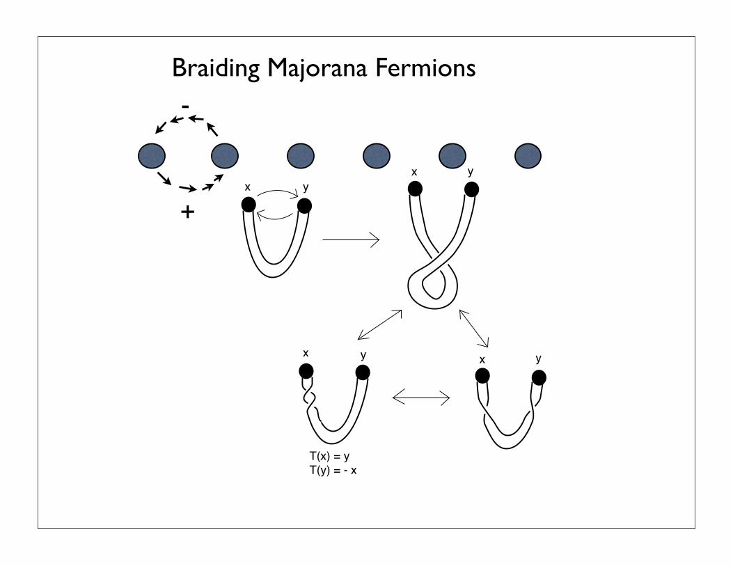
Braiding Majorana Fermions
T(x) = y
T(y) = - x
x
x
xx
y
y
y
y
Figure 23: Braiding Action on a Pair of Fermions
T (p) = sps−1 = (1 + yx√
2)p(
1− yx√2
),
and verify that T (x) = y and T (y) = −x. Now view Figure 23 where we have illustrated atopological interpretation for the braiding of two fermions. In the topological interpretation the
two fermions are connected by a flexible belt. On interchange, the belt becomes twisted by 2π.In the topological interpretation a twist of 2π corresponds to a phase change of −1. (For moreinformation on this topological interpretation of 2π rotation for fermions, see [45].) Without afurther choice it is not evident which particle of the pair should receive the phase change. The
topology alone tells us only the relative change of phase between the two particles. The Clifford
algebra for Majorana fermions makes a specific choice in the matter and in this way fixes the
representation of the braiding.
Finally, we remark that linear combinations of products in the Clifford algebra can be re-
garded as superpositions of the knot sets. Thus xy + xz is a superposition of the sets withmembers x, y andx, z. Superposition of sets suggests that we are creating a species of quan-tum set theory and indeed Clifford algebra based quantum set theories have been suggested (see
[19]) by David Finkelstein and others. It may come as a surprise to a quantum set theorist to find
that knot theoretic topology is directly related to this subject. It is also clear that this Clifford
algebraic quantum set theory should be related to our previous constructions for quantum knots
[60, 61, 62, 63, 64]. This requires more investigation, and it suggests that knot theory and the
theory of braids occupy a fundamental place in the foundations of quantum mechanics.
26


And From Logic Alone?

TRACTATUS LOGICO-PHILOSOPHICUS
a formal law, according to which those propositions are con-structed. In this case the terms of the expression in brackets areall the terms of a formal series.
5.502 Therefore I write instead of “(– – – – –T)(, . . . .)”, “N()”.N() is the negation of all the values of the propositional
variable .
5.503 As it is obviously easy to express how propositions can be con-structed by means of this operation and how propositions arenot to be constructed by means of it, this must be capable ofexact expression.
5.51 If has only one value, then N() = p (not p), if it has twovalues then N() = p . q (neither p nor q).
5.511 How can the all-embracing logic which mirrors the world usesuch special catches and manipulations? Only because all theseare connected into an infinitely fine network, to the great mirror.
5.512 “p” is true if “p” is false. Therefore in the true proposition“p” “p” is a false proposition. How then can the stroke “”bring it into agreement with reality?
That which denies in “p” is however not “”, but that whichall signs of this notation, which deny p, have in common.
Hence the common rule according to which “p”, “p”,“pp”, “p .p”, etc. etc. (to infinity) are constructed. Andthis which is common to them all mirrors denial.
5.513 We could say: What is common to all symbols, which assertboth p and q, is the proposition “p . q”. What is common to allsymbols, which assert either p or q, is the proposition “p q”.
And similarly we can say: Two propositions are opposedto one another when they have nothing in common with oneanother; and every proposition has only one negative, becausethere is only one proposition which lies altogether outside it.
Thus even in Russell’s notation it is evident that “q : pp”says the same as “q”; that “p p” says nothing.
5.514 If a notation is fixed, there is in it a rule according to whichall the propositions denying p are constructed, a rule accordingto which all the propositions asserting p are constructed, a rule
67
TRACTATUS LOGICO-PHILOSOPHICUS
It is clear that logic may not collide with its application.But logic must have contact with its application.Therefore logic and its application may not overlap one an-
other.
5.5571 If I cannot give elementary propositions a priori then it mustlead to obvious nonsense to try to give them.
5.6 The limits of my language mean the limits of my world.
5.61 Logic fills the world: the limits of the world are also its limits.We cannot therefore say in logic: This and this there is in
the world, that there is not.For that would apparently presuppose that we exclude cer-
tain possibilities, and this cannot be the case since otherwiselogic must get outside the limits of the world: that is, if it couldconsider these limits from the other side also.
What we cannot think, that we cannot think: we cannottherefore say what we cannot think.
5.62 This remark provides a key to the question, to what extent solip-sism is a truth.
In fact what solipsism means, is quite correct, only it cannotbe said, but it shows itself.
That the world is my world, shows itself in the fact that thelimits of the language (the language which only I understand)mean the limits of my world.
5.621 The world and life are one.
5.63 I am my world. (The microcosm.)
5.631 The thinking, presenting subject; there is no such thing.If I wrote a book “The world as I found it”, I should also have
therein to report on my body and say which members obey mywill and which do not, etc. This then would be a method ofisolating the subject or rather of showing that in an importantsense there is no subject: that is to say, of it alone in this bookmention could not be made.
5.632 The subject does not belong to the world but it is a limit of theworld.
74
Tractatus Logico-Philosophicus
PREFACE
This book will perhaps only be understood by those who have them-selves already thought the thoughts which are expressed in it—or similarthoughts. It is therefore not a text-book. Its object would be attainedif there were one person who read it with understanding and to whom itaorded pleasure.
The book deals with the problems of philosophy and shows, as Ibelieve, that the method of formulating these problems rests on the mis-understanding of the logic of our language. Its whole meaning could besummed up somewhat as follows: What can be said at all can be saidclearly; and whereof one cannot speak thereof one must be silent.
The book will, therefore, draw a limit to thinking, or rather—not tothinking, but to the expression of thoughts; for, in order to draw a limitto thinking we should have to be able to think both sides of this limit(we should therefore have to be able to think what cannot be thought).
The limit can, therefore, only be drawn in language and what lies onthe other side of the limit will be simply nonsense.
How far my eorts agree with those of other philosophers I will notdecide. Indeed what I have here written makes no claim to novelty inpoints of detail; and therefore I give no sources, because it is indierentto me whether what I have thought has already been thought before meby another.
I will only mention that to the great works of Frege and the writingsof my friend Bertrand Russell I owe in large measure the stimulation ofmy thoughts.
If this work has a value it consists in two things. First that in itthoughts are expressed, and this value will be the greater the better thethoughts are expressed. The more the nail has been hit on the head.—Here I am conscious that I have fallen far short of the possible. Simplybecause my powers are insucient to cope with the task.—May otherscome and do it better.
23
Ludwig Wittgenstein
TRACTATUS LOGICO-PHILOSOPHICUS
4.06 Propositions can be true or false only by being pictures of thereality.
4.061 If one does not observe that propositions have a sense inde-pendent of the facts, one can easily believe that true and falseare two relations between signs and things signified with equalrights.
One could then, for example, say that “p” signifies in the trueway what “p” signifies in the false way, etc.
4.062 Can we not make ourselves understood by means of false propo-sitions as hitherto with true ones, so long as we know that theyare meant to be false? No! For a proposition is true, if whatwe assert by means of it is the case; and if by “p” we mean p,and what we mean is the case, then “p” in the new conceptionis true and not false.
4.0621 That, however, the signs “p” and “p” can say the same thing isimportant, for it shows that the sign “” corresponds to nothingin reality.
That negation occurs in a proposition, is no characteristic ofits sense (p = p).
The propositions “p” and “p” have opposite senses, but tothem corresponds one and the same reality.
4.063 An illustration to explain the concept of truth. A black spot onwhite paper; the form of the spot can be described by sayingof each point of the plane whether it is white or black. To thefact that a point is black corresponds a positive fact; to the factthat a point is white (not black), a negative fact. If I indicatea point of the plane (a truth-value in Frege’s terminology), thiscorresponds to the assumption proposed for judgment, etc. etc.
But to be able to say that a point is black or white, I mustfirst know under what conditions a point is called white or black;in order to be able to say “p” is true (or false) I must havedetermined under what conditions I call “p” true, and thereby Idetermine the sense of the proposition.
The point at which the simile breaks down is this: we canindicate a point on the paper, without knowing what white andblack are; but to a proposition without a sense corresponds noth-ing at all, for it signifies no thing (truth-value) whose properties
43
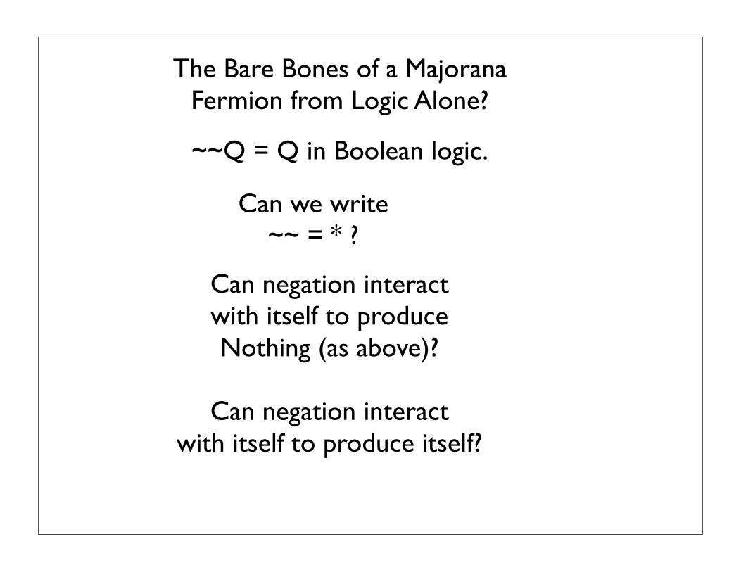
~~Q = Q in Boolean logic.
Can we write ~~ = * ?
Can negation interactwith itself to produce Nothing (as above)?
Can negation interact with itself to produce itself?
The Bare Bones of a Majorana Fermion from Logic Alone?
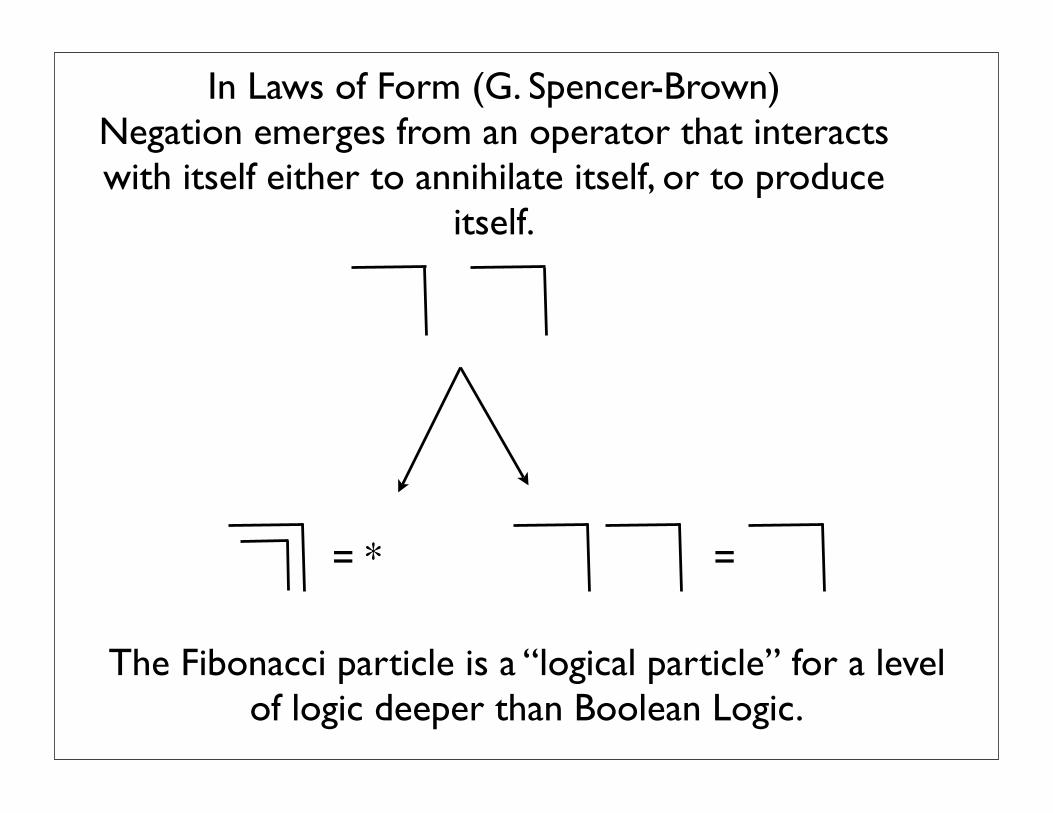
In Laws of Form (G. Spencer-Brown)Negation emerges from an operator that interacts with itself either to annihilate itself, or to produce
itself.
== *
The Fibonacci particle is a “logical particle” for a level of logic deeper than Boolean Logic.

A ~A
AB A or B
True
False* =
Interpretation for Logic


Returning to Square Root of -1, Time and Dirac

Figure 27: Calling, Crossing and Cobordism
5.1 The Square Root of Minus One is an Eigenform and a Clock
So far we have seen that the mark can represent the fusion rules for a Majorana fermion since
it can interact with itself to produce either itself or nothing. But we have not yet seen the anti-
commuting fermion algebra emerge from this context of making a distinction. Remarkably, this
algebra does emerge when one looks at the mark recursively.
Consider the transformation
F (X) = X .
If we iterate it and take the limit we find
G = F (F (F (F (· · ·)))) = ...
an infinite nest of marks satisfying the equation
G = G .
WithG = F (G), I say thatG is an eigenform for the transformation F. See [] for more about thispoint of view. See Figure 28 for an illustration of this nesting with boxes and an arrow that points
inside the reentering mark to indicate its appearance inside itself. If one thinks of the mark itself
as a Boolean logical value, then extending the language to include the reentering mark G goes
beyond the boolean. We will not detail here how this extension can be related to non-standard
logics, but refer the reader to [39]. Taken at face value the reentering mark cannot be just marked
or just unmarked, for by its very definition, if it is marked then it is unmarked and if it is unmarked
then it is marked. In this sense the reentering mark has the form of a self-contradicting paradox.
33
... =
Figure 28:
There is no paradox since we do not have to permanently assign it to either value. The simplest
interpretation of the reentering mark is that it is temporal and that it represents an oscillation
between markedness and unmarkedness. In numerical terms it is a discrete dynamical system
oscillating between +1 (marked) and −1 (not marked).
With the reentering mark in mind consider now the transformation on real numbers given by
T (x) = −1/x.
This has the fixed points i and −i, the complex numbers whose squares are negative unity. Butlets take a point of view more directly associated with the analogy of the recursive mark. Begin
by starting with a simple periodic process that is associated directly with the classical attempt to
solve for i as a solution to a quadratic equation. We take the point of view that solving x2 = ax+bis the same (when x = 0) as solving
x = a + b/x,
and hence is a matter of finding a fixed point. In the case of i we have
x2 = −1
and so desire a fixed point
x = −1/x.
There are no real numbers that are fixed points for this operator and so we consider the oscillatory
process generated by
T (x) = −1/x.
The fixed point would satisfy
i = −1/i
and multiplying, we get that
ii = −1.
On the other hand the iteration of T yields
1, T (1) = −1, T (T (1)) = +1, T (T (T (1))) = −1,+1,−1,+1,−1, · · · .
34
Emergence of Fermion Algebra fromDiscrete Dynamical Process

Volume 4 · Number 3 · July 2009 125
concepts in second-order cyberneticsMathematical
of the world in which we operate. They attaintheir stability through the limiting processthat goes outside the immediate world ofindividual actions. We make an imaginativeleap to complete such objects to becometokens for eigenbehaviors. It is impossible tomake an infinite nest of boxes. We do notmake it. We imagine it. And in imagining thatinfinite nest of boxes, we arrive at the eigen-form.
The leap of imagination to the infiniteeigenform is a model of the human ability tocreate signs and symbols. In the case of theeigenform X with X = F(X), X can be regardedas the name of the process itself or as the nameof the limiting process. Note that if you aretold that
X = F(X),
then, substituting F(X) for X, you can write
X = F(F(X)).
Substituting again and again, you have
X = F(F(F(X))) = F(F(F(F(X)))) = F(F(F(F(F(X))))) = …
The process arises from the symbolicexpression of its eigenform. In this view, theeigenform is an implicate order for the processthat generates it. (Here we refer to implicateorder in the sense of David Bohm 1980).
Sometimes one stylizes the structure byindicating where the eigenform X reenters itsown indicational space with an arrow or othergraphical device. See the picture below for thecase of the nested boxes.
Does the infinite nest of boxes exist? Cer-tainly it does not exist on this page or any-where in the physical world with which we arefamiliar. The infinite nest of boxes exists in theimagination. It is a symbolic entity.
The eigenform is the imagined boundaryin the reciprocal relationship of the object(the “It”) and the process leading to the object(the process leading to “It”). In the diagram
below we have indicated these relationshipswith respect to the eigenform of nested boxes.Note that the “It” is illustrated as a finiteapproximation (to the infinite limit) that issufficient to allow an observer to infer/per-ceive the generating process that underlies it.
Just so, an object in the world (cognitive,physical, ideal, etc.) provides a conceptualcenter for the exploration of a skein of rela-tionships related to its context and to theprocesses that generate it. An object can havevarying degrees of reality, just as an eigenformdoes. If we take the suggestion to heart thatobjects are tokens for eigenbehaviors, then anobject in itself is an entity, participating in anetwork of interactions, taking on its appar-ent solidity and stability from theseinteractions.
An object is an amphibian between thesymbolic and imaginary world of the mindand the complex world of personal experi-ence. The object, when viewed as a process, isa dialogue between these worlds. The object,when seen as a sign for itself, or in and of itself,is imaginary.
Why are objects apparently solid? Ofcourse you cannot walk through a brick walleven if you think about it differently. I do notmean apparent in the sense of thought alone.I mean apparent in the sense of appearance.The wall appears solid to me because of the
actions that I can perform. The wall is quitetransparent to a neutrino, and will not even bean eigenform for that neutrino.
This example shows quite sharply how thenature of an object is entailed in the proper-ties of its observer.
The eigenform model can be expressed inquite abstract and general terms. Supposethat we are given a recursion (not necessarilynumerical) with the equation
X(t + 1) = F(X(t)).
Here X(t) denotes the condition of obser-vation at time t. X(t) could be as simple as aset of nested boxes, or as complex as the entireconfiguration of your body in relation to theknown universe at time t. Then F(X(t))denotes the result of applying the operationssymbolized by F to the condition at time t. Youcould, for simplicity, assume that F is inde-pendent of time. Time independence of therecursion F will give us simple answers and wecan later discuss what will happen if theactions depend upon the time. In the time-independent case we can write
J = F(F(F(…)))
– the infinite concatenation of F upon itself.Then
F(J) = J
since adding one more F to the concatenationchanges nothing.
Thus J, the infinite concatenation of theoperation upon itself leads to a fixed point forF. J is said to be the eigenform for the recur-sion F. We see that every recursion has aneigenform. Every recursion has an (imagi-nary) fixed point.
We end this section with one more exam-ple. This is the eigenform of the Koch fractal(Mandelbrot 1982). In this case one can writesymbolically the eigenform equation
K = K K K K
to indicate that the Koch Fractal reenters itsown indicational space four times (that is, it ismade up of four copies of itself, each one-third the size of the original. The curly brack-ets in the center of this equation refer to thefact that the two middle copies within thefractal are inclined with respect to oneanother and with respect to the two outercopies. In the figure below we show the geo-metric configuration of the reentry.
… =
The It
The Process leading to It... +1, -1, +1, -1, +1, -1, ...
[-1,+1] [+1,-1]
ii = -1i = -1/i
The square rootof minus one
“is”a discrete oscillation.
i as an imaginary value, defined in terms of itself.
THE SQUARE ROOT OF MINUS ONE IS A CLOCK.
From G = G to i = -1/i.

... +1, -1, +1, -1, +1, -1, +1, -1, ...
[-1,+1] [+1,-1]
Figure 29:
The square root of minus one is a perfect example of an eigenform that occurs in a new and wider
domain than the original context in which its recursive process arose. The process has no fixed
point in the original domain.
Looking at the oscillation between +1 and −1, we see that there are naturally two phase-shifted viewpoints. We denote these two views of the oscillation by [+1,−1] and[−1,+1]. Theseviewpoints correspond to whether one regards the oscillation at time zero as starting with +1 orwith −1. See Figure 29. We shall let the word iterant stand for an undisclosed alternation orambiguity between +1 and −1. There are two iterant views: [+1,−1] and [−1,+1] for the basicprocess we are examining. Given an iterant [a, b], we can think of [b, a] as the same process witha shift of one time step. The two iterant views, [+1,−1] and [−1,+1], will become the squareroots of negative unity, i and −i.
We introduce a temporal shift operator η such that
[a, b]η = η[b, a]
and
ηη = 1
for any iterant [a, b], so that concatenated observations can include a time step of one-half periodof the process
· · · abababab · · · .
We combine iterant views term-by-term as in
[a, b][c, d] = [ac, bd].
We now define i by the equation
i = [1,−1]η.
This makes i both a value and an operator that takes into account a step in time.
We calculate
ii = [1,−1]η[1,−1]η = [1,−1][−1, 1]ηη = [−1,−1] = −1.
35
T(x) = -1/x
Fixed Point: i = -1/i
From G = G to i = -1/i.
The Square Root of Minus One is a Clock.

... +1, -1, +1, -1, +1, -1, +1, -1, ...
[-1,+1] [+1,-1]
Figure 29:
The square root of minus one is a perfect example of an eigenform that occurs in a new and wider
domain than the original context in which its recursive process arose. The process has no fixed
point in the original domain.
Looking at the oscillation between +1 and −1, we see that there are naturally two phase-shifted viewpoints. We denote these two views of the oscillation by [+1,−1] and[−1,+1]. Theseviewpoints correspond to whether one regards the oscillation at time zero as starting with +1 orwith −1. See Figure 29. We shall let the word iterant stand for an undisclosed alternation orambiguity between +1 and −1. There are two iterant views: [+1,−1] and [−1,+1] for the basicprocess we are examining. Given an iterant [a, b], we can think of [b, a] as the same process witha shift of one time step. The two iterant views, [+1,−1] and [−1,+1], will become the squareroots of negative unity, i and −i.
We introduce a temporal shift operator η such that
[a, b]η = η[b, a]
and
ηη = 1
for any iterant [a, b], so that concatenated observations can include a time step of one-half periodof the process
· · · abababab · · · .
We combine iterant views term-by-term as in
[a, b][c, d] = [ac, bd].
We now define i by the equation
i = [1,−1]η.
This makes i both a value and an operator that takes into account a step in time.
We calculate
ii = [1,−1]η[1,−1]η = [1,−1][−1, 1]ηη = [−1,−1] = −1.
35
and
ηη = 1
for any iterant [a, b], so that concatenated observations can include a time step of one-half periodof the process
· · ·abababab · · · .
We combine iterant views term-by-term as in
[a, b][c, d] = [ac, bd].
We now define i by the equation
i = [1,−1]η.
This makes i both a value and an operator that takes into account a step in time.
We calculate
ii = [1,−1]η[1,−1]η = [1,−1][−1, 1]ηη = [−1,−1] = −1.
Thus we have constructed a square root of minus one by using an iterant viewpoint. In this view
i represents a discrete oscillating temporal process and it is an eigenform for T (x) = −1/x,participating in the algebraic structure of the complex numbers. In fact the corresponding algebra
structure of linear combinations [a, b]+[c, d]η is isomorphic with 2×2matrix algebra and iterantscan be used to construct n × n matrix algebra. We treat this generalization elsewhere [72, 73].
Now we can make contact with the algebra of the Majorana fermions. Let e = [1,−1]. Thenwe have e2 = [1, 1] = 1 and eη = [1,−1]η = [−1, 1]η = −eη. Thus we have
e2 = 1,
η2 = 1,
and
eη = −ηe.
We can regard e and η as a fundamental pair of Majorana fermions. This is a formal corre-spondence, but it is striking how this Marjorana fermion algebra emerges from an analysis of
the recursive nature of the reentering mark, while the fusion algebra for the Majorana fermion
emerges from the distinctive properties of the mark itself. We see how the seeds of the fermion
algebra live in this extended logical context.
Note how the development of the algebra works at this point. We have that
(eη)2 = −1
and so regard this as a natural construction of the square root of minus one in terms of the phase
synchronization of the clock that is the iteration of the reentering mark. Once we have the square
36
and
ηη = 1
for any iterant [a, b], so that concatenated observations can include a time step of one-half periodof the process
· · ·abababab · · · .
We combine iterant views term-by-term as in
[a, b][c, d] = [ac, bd].
We now define i by the equation
i = [1,−1]η.
This makes i both a value and an operator that takes into account a step in time.
We calculate
ii = [1,−1]η[1,−1]η = [1,−1][−1, 1]ηη = [−1,−1] = −1.
Thus we have constructed a square root of minus one by using an iterant viewpoint. In this view
i represents a discrete oscillating temporal process and it is an eigenform for T (x) = −1/x,participating in the algebraic structure of the complex numbers. In fact the corresponding algebra
structure of linear combinations [a, b]+[c, d]η is isomorphic with 2×2matrix algebra and iterantscan be used to construct n × n matrix algebra. We treat this generalization elsewhere [72, 73].
Now we can make contact with the algebra of the Majorana fermions. Let e = [1,−1]. Thenwe have e2 = [1, 1] = 1 and eη = [1,−1]η = [−1, 1]η = −eη. Thus we have
e2 = 1,
η2 = 1,
and
eη = −ηe.
We can regard e and η as a fundamental pair of Majorana fermions. This is a formal corre-spondence, but it is striking how this Marjorana fermion algebra emerges from an analysis of
the recursive nature of the reentering mark, while the fusion algebra for the Majorana fermion
emerges from the distinctive properties of the mark itself. We see how the seeds of the fermion
algebra live in this extended logical context.
Note how the development of the algebra works at this point. We have that
(eη)2 = −1
and so regard this as a natural construction of the square root of minus one in terms of the phase
synchronization of the clock that is the iteration of the reentering mark. Once we have the square
36

and
ηη = 1
for any iterant [a, b], so that concatenated observations can include a time step of one-half periodof the process
· · ·abababab · · · .
We combine iterant views term-by-term as in
[a, b][c, d] = [ac, bd].
We now define i by the equation
i = [1,−1]η.
This makes i both a value and an operator that takes into account a step in time.
We calculate
ii = [1,−1]η[1,−1]η = [1,−1][−1, 1]ηη = [−1,−1] = −1.
Thus we have constructed a square root of minus one by using an iterant viewpoint. In this view
i represents a discrete oscillating temporal process and it is an eigenform for T (x) = −1/x,participating in the algebraic structure of the complex numbers. In fact the corresponding algebra
structure of linear combinations [a, b]+[c, d]η is isomorphic with 2×2matrix algebra and iterantscan be used to construct n × n matrix algebra. We treat this generalization elsewhere [72, 73].
Now we can make contact with the algebra of the Majorana fermions. Let e = [1,−1]. Thenwe have e2 = [1, 1] = 1 and eη = [1,−1]η = [−1, 1]η = −eη. Thus we have
e2 = 1,
η2 = 1,
and
eη = −ηe.
We can regard e and η as a fundamental pair of Majorana fermions. This is a formal corre-spondence, but it is striking how this Marjorana fermion algebra emerges from an analysis of
the recursive nature of the reentering mark, while the fusion algebra for the Majorana fermion
emerges from the distinctive properties of the mark itself. We see how the seeds of the fermion
algebra live in this extended logical context.
Note how the development of the algebra works at this point. We have that
(eη)2 = −1
and so regard this as a natural construction of the square root of minus one in terms of the phase
synchronization of the clock that is the iteration of the reentering mark. Once we have the square
36
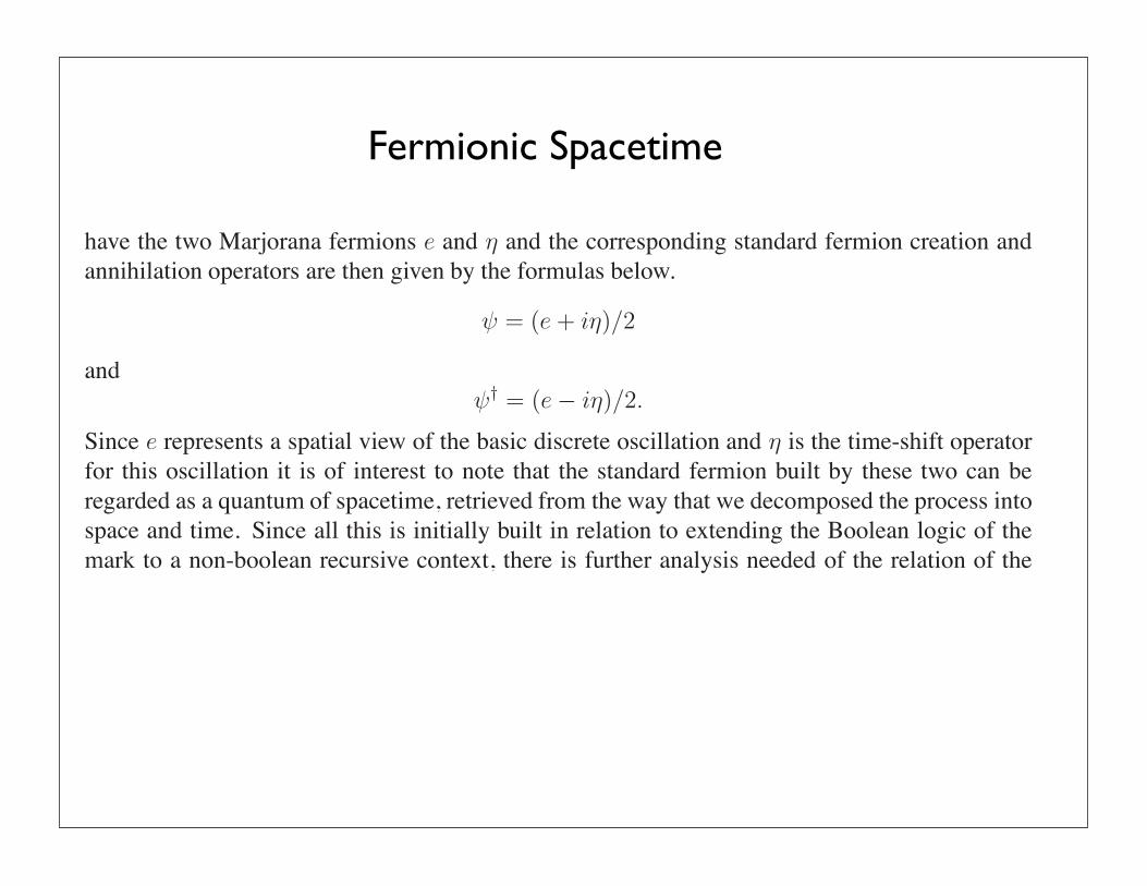
There is one more comment that is appropriate for this section. Recall from Section 4 that a
pair of Majorana fermions can be assembled to form a single standard fermion. In our case we
have the two Marjorana fermions e and η and the corresponding standard fermion creation andannihilation operators are then given by the formulas below.
ψ = (e + iη)/2
and
ψ† = (e− iη)/2.
Since e represents a spatial view of the basic discrete oscillation and η is the time-shift operatorfor this oscillation it is of interest to note that the standard fermion built by these two can be
regarded as a quantum of spacetime, retrieved from the way that we decomposed the process into
space and time. Since all this is initially built in relation to extending the Boolean logic of the
mark to a non-boolean recursive context, there is further analysis needed of the relation of the
physics and the logic. This will be taken up in a separate paper.
5.2 Relativity and the Dirac Equation
Starting with the algebra structure of e and η and adding a commuting square root of −1, i, wehave constructed fermion algebra and quaternion algebra. We can now go further and construct
the Dirac equation. This may sound circular, in that the fermions arise from solving the Dirac
equation, but in fact the algebra underlying this equation has the same properties as the creation
and annihilation algebra for fermions, so it is by way of this algebra that we will come to the
Dirac equation. If the speed of light is equal to 1 (by convention), then energy E, momentum pand massm are related by the (Einstein) equation
E2 = p2 +m2.
Dirac constructed his equation by looking for an algebraic square root of p2+m2 so that he could
have a linear operator for E that would take the same role as the Hamiltonian in the Schrodinger
equation. We will get to this operator by first taking the case where p is a scalar (we use onedimension of space and one dimension of time. Let E = αp + βm where α and β are elementsof a a possibly non-commutative, associative algebra. Then
E2 = α2p2 + β2m2 + pm(αβ + βα).
Hence we will satisfiy E2 = p2 + m2 if α2 = β2 = 1 and αβ + βα = 0. This is our familiarClifford algebra pattern and we can use the iterant algebra generated by e and η if we wish. Then,because the quantum operator for momentum is−i∂/∂x and the operator for energy is i∂/∂t, wehave the Dirac equation
i∂ψ/∂t = −iα∂ψ/∂x + βmψ.
Let
O = i∂/∂t + iα∂/∂x − βm
37
Fermionic Spacetime
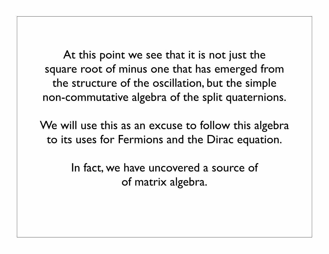
At this point we see that it is not just the square root of minus one that has emerged from
the structure of the oscillation, but the simple non-commutative algebra of the split quaternions.
We will use this as an excuse to follow this algebra to its uses for Fermions and the Dirac equation.
In fact, we have uncovered a source of of matrix algebra.

[a,b] + [c,d]!
and it is not hard to see that this is isomorphic with 2 x 2 matrix algebra with the correspondence given by the diagram below.
[a,b] + [c,d] a c
d b!
Figure 23 We see from this excursion that there is a full interpretation for the complex numbers (and indeed matrix algebra) as an observational system taking into account time shifts for underlying iterant processes. Let A = [a,b] and B = [c,d] and let C = [r,s], D = [t,u]. With A' = [b,a], we have
(A + B!)(C+D!) = (AC + BD') + (AD + BC')! .
This writes 2 x 2 matrix algebra in the form of a hypercomplex number system. From the point of view of iterants, the sum [a,b] + [b,c]! can be regarded as a superposition of two types of
observation of the iterants Ia,b and Ic,d. The operator-view [c,d]! includes the shift that will move the viewpoint from
[c,d] to [d,c], while [a,b] does not contain this shift. Thus a shift of viewpoint on [c,d] in this superposition does not affect the values of [a,b]. One can think of the corresponding process as having the form shown below.
... a a a a a a a a a a a a a a a ... ... c d c d c d c d c d c d c d ...
... b b b b b b b b b b b b b b ... The snapshot [c,d] changes to [d,c] in the horizontal time-shift while the vertical snapshot [a,b] remains invariant under the shift. It is interesting to note that in the spatial explication of the process we can imagine the horizontal oscillation corresponding to [c,d]!
as making a boundary (like a frieze pattern), while the vertical iterant parts a and b mark the two sides of that boundary.

root of minus one it is natural to introduce another one and call this one i, letting it commute withthe other operators. Then we have the (ieη)2 = +1 and so we have a triple of Majorana fermions:
a = e, b = η, c = ieη
and we can construct the quaternions
I = ba = ηe, J = cb = ie, K = ac = iη.
With the quaternions in place, we have the braiding operators
A =1√2(1 + I), B =
1√2(1 + J), C =
1√2(1 + K),
and can continue as we did in Section 4.
There is one more comment that is appropriate for this section. Recall from Section 4 that a
pair of Majorana fermions can be assembled to form a single standard fermion. In our case we
have the two Marjorana fermions e and η and the corresponding standard fermion annihilationand creation operators are then given by the formulas below.
ψ = (e + iη)/2
and
ψ† = (e − iη)/2.
Since e represents a spatial view of the basic discrete oscillation and η is the time-shift operatorfor this oscillation it is of interest to note that the standard fermion built by these two can be
regarded as a quantum of spacetime, retrieved from the way that we decomposed the process into
space and time. Since all this is initially built in relation to extending the Boolean logic of the
mark to a non-boolean recursive context, there is further analysis needed of the relation of the
physics and the logic. This will be taken up in a separate paper.
5.2 Relativity and the Dirac Equation
Starting with the algebra structure of e and η and adding a commuting square root of −1, i, wehave constructed fermion algebra and quaternion algebra. We can now go further and construct
the Dirac equation. This may sound circular, in that the fermions arise from solving the Dirac
equation, but in fact the algebra underlying this equation has the same properties as the creation
and annihilation algebra for fermions, so it is by way of this algebra that we will come to the
Dirac equation. If the speed of light is equal to 1 (by convention), then energy E, momentum pand massm are related by the (Einstein) equation
E2 = p2 + m2.
37

Dirac constructed his equation by looking for an algebraic square root of p2 +m2 so that he could
have a linear operator for E that would take the same role as the Hamiltonian in the Schrodinger
equation. We will get to this operator by first taking the case where p is a scalar (we use onedimension of space and one dimension of time. Let E = αp + βm where α and β are elementsof a a possibly non-commutative, associative algebra. Then
E2 = α2p2 + β2m2 + pm(αβ + βα).
Hence we will satisfiy E2 = p2 + m2 if α2 = β2 = 1 and αβ + βα = 0. This is our familiarClifford algebra pattern and we can use the iterant algebra generated by e and η if we wish. Then,because the quantum operator for momentum is−i∂/∂x and the operator for energy is i∂/∂t, wehave the Dirac equation
i∂ψ/∂t = −iα∂ψ/∂x + βmψ.
Let
O = i∂/∂t + iα∂/∂x − βm
so that the Dirac equation takes the form
Oψ(x, t) = 0.
Now note that
Oei(px−Et) = (E − αp + βm)ei(px−Et)
and that if
U = (E − αp + βm)βα = βαE + βp + αm,
then
U2 = −E2 + p2 + m2 = 0,
from which it follows that
ψ = Uei(px−Et)
is a (plane wave) solution to the Dirac equation.
In fact, this calculation suggests that we should multiply the operator O by βα on the right,obtaining the operator
D = Oβα = iβα∂/∂t + iβ∂/∂x + αm,
and the equivalent Dirac equation
Dψ = 0.
In fact for the specific ψ above we will now have D(Uei(px−Et)) = U2ei(px−Et) = 0. This wayof reconfiguring the Dirac equation in relation to nilpotent algebra elements U is due to Peter
Rowlands [94]. We will explore this relationship with the Rowlands formulation in a separate
paper.
38
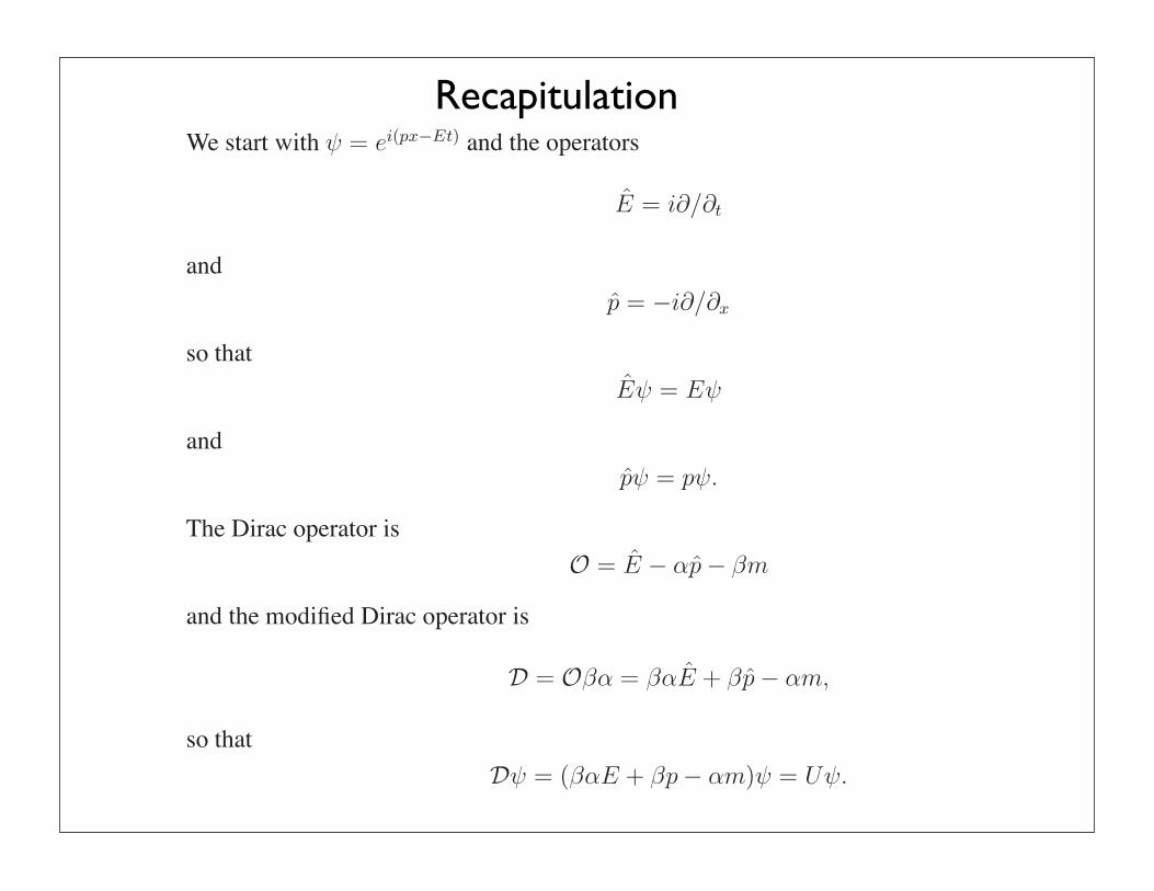
9.1 Another version of U and U †
We start with ψ = ei(px−Et) and the operators
E = i∂/∂t
and
p = −i∂/∂x
so that
Eψ = Eψ
and
pψ = pψ.
The Dirac operator is
O = E − αp − βm
and the modified Dirac operator is
D = Oβα = βαE + βp − αm,
so that
Dψ = (βαE + βp − αm)ψ = Uψ.
If we let
ψ = ei(px+Et)
(reversing time), then we have
Dψ = (−βαE + βp − αm)ψ = U †ψ,
giving a definition of U † corresponding to the anti-particle for Uψ.
We have that
U2 = U †2 = 0
and
UU † + U †U = 4E2.
Thus we have a direct appearance of the Fermion algebra corresponding to the Fermion plane
wave solutions to the Dirac equation.
38
Recapitulation
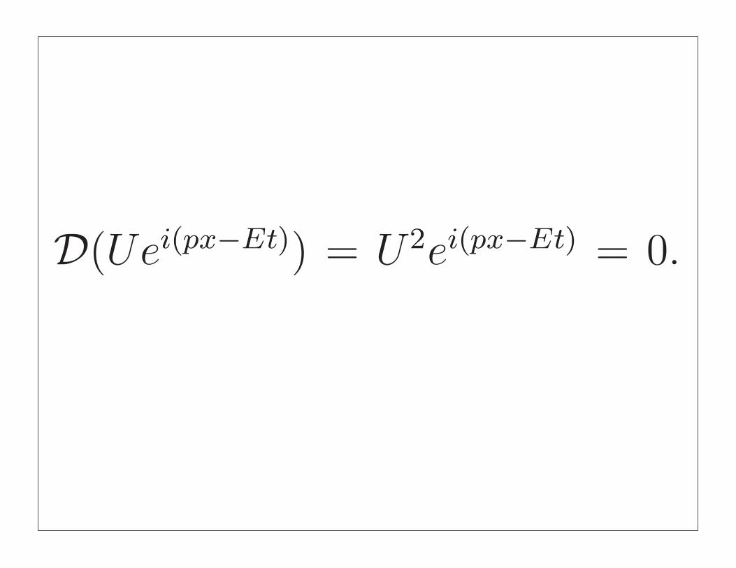
Dirac constructed his equation by looking for an algebraic square root of p2 +m2 so that he could
have a linear operator for E that would take the same role as the Hamiltonian in the Schrodinger
equation. We will get to this operator by first taking the case where p is a scalar (we use onedimension of space and one dimension of time. Let E = αp + βm where α and β are elementsof a a possibly non-commutative, associative algebra. Then
E2 = α2p2 + β2m2 + pm(αβ + βα).
Hence we will satisfiy E2 = p2 + m2 if α2 = β2 = 1 and αβ + βα = 0. This is our familiarClifford algebra pattern and we can use the iterant algebra generated by e and η if we wish. Then,because the quantum operator for momentum is−i∂/∂x and the operator for energy is i∂/∂t, wehave the Dirac equation
i∂ψ/∂t = −iα∂ψ/∂x + βmψ.
Let
O = i∂/∂t + iα∂/∂x − βm
so that the Dirac equation takes the form
Oψ(x, t) = 0.
Now note that
Oei(px−Et) = (E − αp + βm)ei(px−Et)
and that if
U = (E − αp + βm)βα = βαE + βp + αm,
then
U2 = −E2 + p2 + m2 = 0,
from which it follows that
ψ = Uei(px−Et)
is a (plane wave) solution to the Dirac equation.
In fact, this calculation suggests that we should multiply the operator O by βα on the right,obtaining the operator
D = Oβα = iβα∂/∂t + iβ∂/∂x + αm,
and the equivalent Dirac equation
Dψ = 0.
In fact for the specific ψ above we will now have D(Uei(px−Et)) = U2ei(px−Et) = 0. This wayof reconfiguring the Dirac equation in relation to nilpotent algebra elements U is due to Peter
Rowlands [94]. We will explore this relationship with the Rowlands formulation in a separate
paper.
38

9.1 Another version of U and U †
We start with ψ = ei(px−Et) and the operators
E = i∂/∂t
and
p = −i∂/∂x
so that
Eψ = Eψ
and
pψ = pψ.
The Dirac operator is
O = E − αp − βm
and the modified Dirac operator is
D = Oβα = βαE + βp − αm,
so that
Dψ = (βαE + βp − αm)ψ = Uψ.
If we let
ψ = ei(px+Et)
(reversing time), then we have
Dψ = (−βαE + βp − αm)ψ = U †ψ,
giving a definition of U † corresponding to the anti-particle for Uψ.
We have that
U2 = U †2 = 0
and
UU † + U †U = 4E2.
Thus we have a direct appearance of the Fermion algebra corresponding to the Fermion plane
wave solutions to the Dirac equation.
38

We have
U = betaαE + βp − αm
and
U † = −βαE + βp − αm
Note that here we have
(U + U †)2 = (2βp + αm)2 = 4(p2 + m2) = 4E2,
and
(U − U †)2 = −(2βαE)2 = −4E2.
We have that
U2 = (U †)2 = 0
and
UU † + U †U = 4E2.
Thus we have a direct appearance of the Fermion algebra corresponding to the Fermion plane
wave solutions to the Dirac equation. Furthermore, the decomposition of Uand U † into the cor-
responding Majorana Fermion operators corresponds to E2 = p2 + m2. Normalizing by dividingby 2E we have
A = (βp + αm)/E
and
B = iβα.
so that
A2 = B2 = 1
and
AB + BA = 0.
then
U = (A + Bi)E
and
U † = (A − Bi)E,
showing how the Fermion operators are expressed in terms of the simpler Clifford algebra of
Majorana operators (split quaternions once again).
9.2 The Majorana Version of the Dirac Equation
∂ψ2/∂r = ψ2
∂ψ1/∂l = −ψ1
39

Note that we get different decompositions of the Fermion into Majorana operators according to what
is reversed.
E and p,m for time reversal.p and E,m for spin reversal.
E,p and m for spin and time reversal.

and
UU † + U †U = 4E2.
Thus we have a direct appearance of the Fermion algebra corresponding to the Fermion plane
wave solutions to the Dirac equation. Furthermore, the decomposition of Uand U † into the cor-
responding Majorana Fermion operators corresponds to E2 = p2 + m2. Normalizing by dividingby 2E we have
A = (βp + αm)/E
and
B = iβα.
so that
A2 = B2 = 1
and
AB + BA = 0.
then
U = (A + Bi)E
and
U † = (A − Bi)E,
showing how the Fermion operators are expressed in terms of the simpler Clifford algebra of
Majorana operators (split quaternions once again).
10.2 Writing in the Full Dirac Algebra
We have written the Dirac equation so far in one dimension of space and one dimension of
time. We give here a way to boost the formalism directly to three dimensions of space. We
take an independent Clifford algebra generated by σ1, σ2, σ3 with σ2i = 1 for i = 1, 2, 3 and
σiσj = −σjσi for i = j. Now assume that α and β as we have used them above generate
an independent Clifford algebra that commutes with the algebra of the σi. Replace the scalarmomentum p by a 3-vector momentum p = (p1, p2, p3) and let p • σ = p1σ1 + p2σ2 + p3σ3. Wereplace ∂/∂x with ∇ = (∂/∂x1, ∂/∂x2, ∂/∂x2) and ∂p/∂x with∇ • p.
We then have the following form of the Dirac equation.
i∂ψ/∂t = −iα∇ • σψ + βmψ.
Let
O = i∂/∂t + iα∇ • σ − βm
so that the Dirac equation takes the form
Oψ(x, t) = 0.
50
Writing in the Full Dirac Algebra
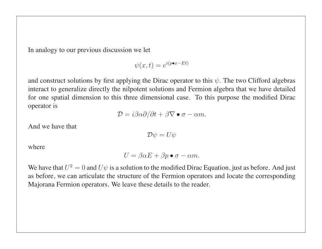
In analogy to our previous discussion we let
ψ(x, t) = ei(p•x−Et)
and construct solutions by first applying the Dirac operator to this ψ. The two Clifford algebrasinteract to generalize directly the nilpotent solutions and Fermion algebra that we have detailed
for one spatial dimension to this three dimensional case. To this purpose the modified Dirac
operator is
D = iβα∂/∂t + β∇ • σ − αm.
And we have that
Dψ = Uψ
where
U = βαE + βp • σ − αm.
We have that U2 = 0 and Uψ is a solution to the modified Dirac Equation, just as before. And justas before, we can articulate the structure of the Fermion operators and locate the corresponding
Majorana Fermion operators. We leave these details to the reader.
10.3 Majorana Fermions at Last
There is more to do. We will end with a brief discussion making Dirac algebra distinct from the
one generated by α, β, σ1, σ2, σ3 to obtain an equation that can have real solutions. This was the
strategy that Majorana [7] followed to construct his Majorana Fermions. A real equation can have
solutions that are invariant under complex conjugation and so can correspond to particles that are
their own anti-particles. We will describe this Majorana algebra in terms of the split quaternions
ϵ and η. For convenience we use the matrix representation given below. The reader of this papercan substitute the corresponding iterants.
ϵ =
!
−1 00 1
"
, η =
!
0 11 0
"
.
Let ϵ and η generate another, independent algebra of split quaternions, commuting with the firstalgebra generated by ϵ and η. Then a totally real Majorana Dirac equation can be written asfollows:
(∂/∂t + ηη∂/∂x + ϵ∂/∂y + ϵη∂/∂z − ϵηηm)ψ = 0.
To see that this is a correct Dirac equation, note that
E = αxpx + αypy + αzpz + βm
(Here the “hats” denote the quantum differential operators corresponding to the energy and mo-
mentum.) will satisfy
E2 = px2 + py
2 + pz2 + m2
51
The Majorana-Dirac Equation
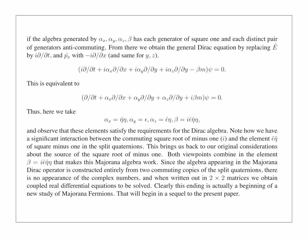
if the algebra generated by αx, αy, αz, β has each generator of square one and each distinct pairof generators anti-commuting. From there we obtain the general Dirac equation by replacing Eby i∂/∂t, and px with −i∂/∂x (and same for y, z).
(i∂/∂t + iαx∂/∂x + iαy∂/∂y + iαz∂/∂y − βm)ψ = 0.
This is equivalent to
(∂/∂t + αx∂/∂x + αy∂/∂y + αz∂/∂y + iβm)ψ = 0.
Thus, here we take
αx = ηη, αy = ϵ, αz = ϵη, β = iϵηη,
and observe that these elements satisfy the requirements for the Dirac algebra. Note how we have
a significant interaction between the commuting square root of minus one (i) and the element ϵηof square minus one in the split quaternions. This brings us back to our original considerations
about the source of the square root of minus one. Both viewpoints combine in the element
β = iϵηη that makes this Majorana algebra work. Since the algebra appearing in the MajoranaDirac operator is constructed entirely from two commuting copies of the split quaternions, there
is no appearance of the complex numbers, and when written out in 2 × 2 matrices we obtaincoupled real differential equations to be solved. Clearly this ending is actually a beginning of a
new study of Majorana Fermions. That will begin in a sequel to the present paper.
References
[1] G. Spencer–Brown, “Laws of Form,” George Allen and Unwin Ltd. London (1969).
[2] Kauffman, L. [1985], Sign and Space, In Religious Experience and Scientific Paradigms.
Proceedings of the 1982 IASWR Conference, Stony Brook, New York: Institute of Ad-
vanced Study of World Religions, (1985), 118-164.
[3] Kauffman, L. [1987], Self-reference and recursive forms, Journal of Social and Biological
Structures (1987), 53-72.
[4] Kauffman, L. [1987], Special relativity and a calculus of distinctions. Proceedings of the
9th Annual Intl. Meeting of ANPA, Cambridge, England (1987). Pub. by ANPA West, pp.
290-311.
[5] Kauffman, L. [1987], Imaginary values in mathematical logic. Proceedings of the Seven-
teenth International Conference on Multiple Valued Logic, May 26-28 (1987), Boston MA,
IEEE Computer Society Press, 282-289.
[6] Kauffman, L. H., Knot Logic, In Knots and Applications ed. by L. Kauffman, World Scien-
tific Pub. Co., (1994), pp. 1-110.
52

The Feynman Checkerboard
where
Czn =
z(z − 1) · · · (z − n + 1)
n!(30)
denotes the choice coefficient.
(r, ) = (7, 0)
x
t
r = (t+x)/2 = (t–x)/2 8131A10
(r, ) = (0, 0)
(r, ) = (7, 3)
(r, ) = (0, 3)
3–96
Figure 1: Rectangular lattice in Minkowski space-time.
We are thinking of r and ℓ as the light cone coordinates r = 12 (t + x), ℓ =
12 (t − x). Hence, in a standard diagram for Minkowski space-time, a pair of values
[r, ℓ] determines a rectangle with sides of length ℓ and r on the left and right pointing
light cones. (We take the speed of light c = 1.) This is shown in Figure. 1.
Clearly, the simplest way to think about this combinatorics is to take ∆ = 1. If
we wish to think about the usual continuum limit, then we shall fix values of r and ℓ
and choose ∆ small but such that r/∆ and ℓ/∆ are integers. The combinatorics of an
r×ℓ rectangle with integers r and ℓ is no different in principle than the combinatorics
of an (r/∆)× (ℓ/∆) rectangle with integers r/∆ and ℓ/∆. Accordingly, we shall take
∆ = 1 for the rest of this discussion, and then make occasional comments to connect
this with the general case.
8
ψ = ΣP iC(P )
Formalism, Metaphor and the Art of Mathematics
Louis H. KauffmanDepartment of Mathematics, Statistics
and Computer Science (m/c 249)851 South Morgan Street
University of Illinois at ChicagoChicago, Illinois 60607-7045
AbstractVoid
1 Introduction = P iC(P )
=((1)1/ 1
1)
This is an essay about Art and Mathematics, written from the point of view of amathematician. In that sense this is an essay about the art of mathematics, not about artas a domain separate from mathematics. And yet ... there is, I believe, a subtle influenceof the arts (music, literature, poetry, painting, sculpture, theatre,...) on mathematics,and concomittantly, an influence of mathematics on these fields of aesthetic action.I can only competently write about the mathematical, but in musing on this themesome opinions will naturally come forth. I had best say a few of them right at theoutset. I firmly believe that the creative source of good art and good mathematics isthe same. I believe that source to be the human desire and need to go across apparentboundaries and find commonality and communication between and among seeminglyseparate domains. In fact, this is the engine of metaphor. Metaphor declares the identityof that which common sense declares different. “Juliet is the sun.” Only in the realmof metaphor can we make such an identification, and yet indeed Juliet and the sunare bound in radience. It is the identification of Juliet and the sun that makes this ametaphor and not an analogy. The declaration of identity wipes away the superficialdifference and directs us to the deep relation beneath the surface.
C(P) = number
of corners in path P
Dirac Amplitude
P
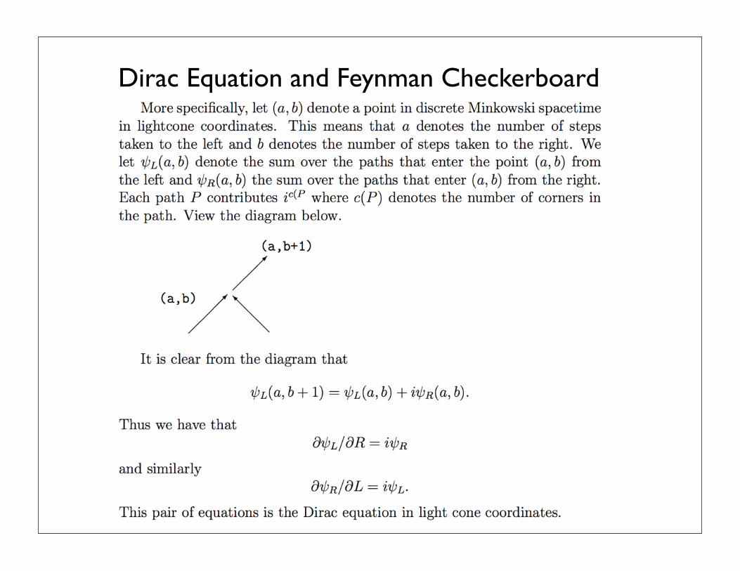
Dirac Equation and Feynman Checkerboard
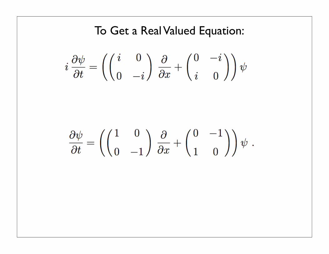
To Get a Real Valued Equation:
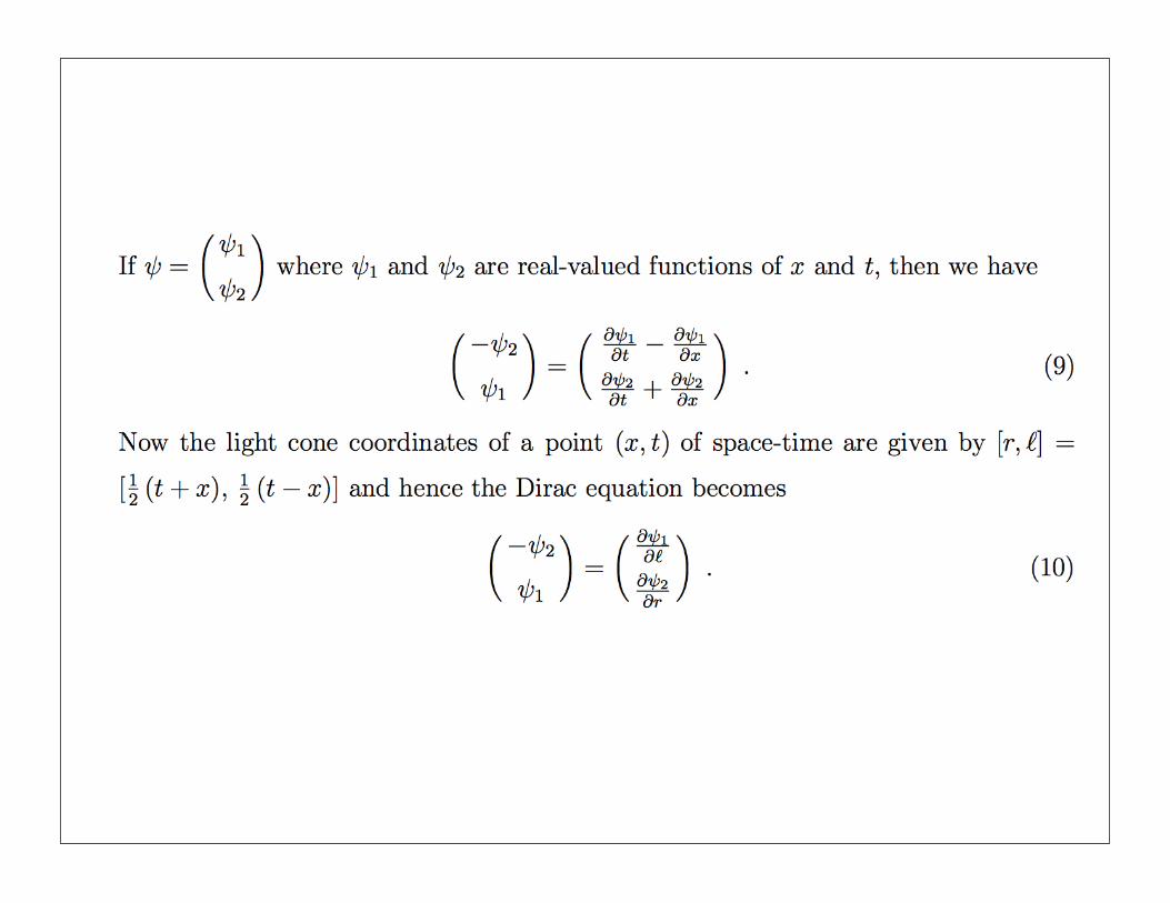

9.2 The Majorana Version of the Dirac Equation
∂ψ2/∂r = ψ2
∂ψ1/∂l = −ψ1
Return now to the original version of the Dirac equation.
i∂ψ/∂t = −iα∂ψ/∂x + βmψ.
We can rewrite this as
∂ψ/∂t = α∂ψ/∂x + iβmψ.
We see that if iβ is real, then we can write a fully real version of the Dirac equation. For example,we can take the equation
∂ψ/∂t = e∂ψ/∂x + eηmψ.
where we represent
e =
!
−1 00 1
"
and
η =
!
0 11 0
"
as matrix versions of the iterants associated with the reentering mark. For the case of one di-
mension of space and one dimension of time, this is the Majorana representation for the Dirac
equation (compare [?]). Since the equation can have real solutions, these are their own complex
conjugates and correspond to particles that are their own anti-particles. As the reader can check,
the corresponding Rowland nilpotent U is given by the formula
U = −iηE + ieηp + em.
For effective application to the topics in this paper, one needs to use two dimensions of space and
one dimension of time.
References
[1] Dyson, F. J. [1990], Feynman’s proof of the Maxwell Equations, Am. J. Phys. 58 (3), March
1990, 209-211.
[2] Connes,Alain [1990], Non-commutative Geometry Academic Press.
[3] Deakin, A.M. [1999] Where does Schroedinger’s equation really come from?, in “Aspects
II - Proceedings of ANPA 20”, edited by K.G. Bowden, published by ANPA.
39
In the RII, Majorana Fermion case we have
Thus the Checkerboard works with plus/minus cornering.This model gives a picture of how Majorana’s
equations can look in an explicit case and show how discrete quantum physics may
avoid complex numbers.
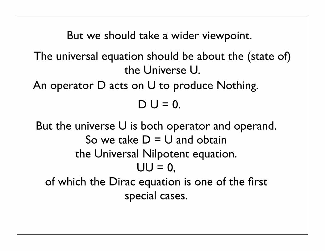
But we should take a wider viewpoint.
The universal equation should be about the (state of) the Universe U.
D U = 0.
But the universe U is both operator and operand.So we take D = U and obtain
the Universal Nilpotent equation.UU = 0,
of which the Dirac equation is one of the first special cases.
An operator D acts on U to produce Nothing.

The Simplest example of the Universal Nilpotent Equationis given by the operator
Ux = x
Here the Universe U is that Universe (self) created by the Mark and taken to
Nothing by the crossing from the marked state to the unmarked state.
UU = =
UU = 0.
.
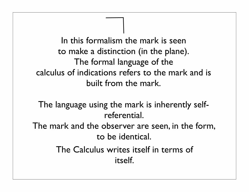
In this formalism the mark is seento make a distinction (in the plane).
The formal language of thecalculus of indications refers to the mark and is
built from the mark.
The language using the mark is inherently self-referential.
The mark and the observer are seen, in the form, to be identical.
The Calculus writes itself in terms of itself.
Physical theory isseen to write itself in terms of the condition
for observation to occur at all.


Discrete Physics and Non-Commtative Frameworks

Discrete Measurement is Intrisically Non-commutative.
Time Series: X, X’, X’’, ...
Here dt and dX are finite increments.
Derivative: X = (X’ -X)/dt = dX/dt
XX: Observe X, then observe X.
XX: Observe X, then observe X.
XX = X’(X’-X)/dtXX = (X’-X)X/dt
XX - XX = (X’-X)(X’-X)/dt
[X,X] = (dX) /dt2

XX - XX = (X’-X)(X’-X)/dt
[X,X] = K then K = (dx)(dx)/dt
X’ = X dx
The discrete analog ofHeisenberg’s equation yields
a Brownian walk with diffusion constant K.

Recalling the Diffusion Constant and the Diffusion Equation
x x+dxx-dx
P(x,t) = Probability that the particle is at x at time t.
P(x,t+dt) = (1/2)[P(x+dx,t) + P(x-dx,t)]
P(x,t+dt) - P(x,t) = (1/2)[P(x+dx,t) - P(x,t) -(P(x,t) - P(x-dx,t))]
,whence
dP/dt = (K/2) d P/dx2 2
K = (dx) /dt2Diffusion Equation
Diffusion Constant
We have just seen the diffusion constant arise differently(!) in the context of discrete process
commutators, with no second difference.
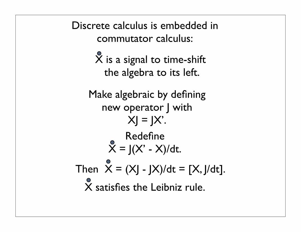
X is a signal to time-shift the algebra to its left.
Make algebraic by defining new operator J with
XJ = JX’.Redefine
X = J(X’ - X)/dt.
Then X = (XJ - JX)/dt = [X, J/dt].
Discrete calculus is embedded incommutator calculus:
X satisfies the Leibniz rule.

A non-commutative world of flat coordinates
suitable for advanced calculus.
The flat coordinates Xi satisfy the equations below with the Pj chosen torepresent di#erentiation with respect to Xj:
[Xi, Xj] = 0,
[Pi, Pj] = 0,
[Xi, Pj] = ij.
Derivatives are represented by commutators.
iF = F/Xi = [F, Pi],
iF = F/Pi = [Xi, F ].
Temporal derivative is represented by commutation with a special (Hamilto-nian) element H of the algebra:
dF/dt = [F, H].
(For quantum mechanics, take ihdA/dt = [A, H].) These non-commutativecoordinates are the simplest flat set of coordinates for description of temporalphenomena in a non-commutative world. Note that Hamilton’s equations area consequence of these definitions. The very short proof of this fact is givenbelow.
Hamilton’s Equations.
dPi/dt = [Pi, H] = [H, Pi] = H/Xi
dXi/dt = [Xi, H] = H/Pi.
These are exactly Hamilton’s equations of motion. The pattern of Hamilton’sequations is built into the system.
Discrete Measurement. Consider a time series X, X , X , · · · with com-muting scalar values. Let
X = X = JDX = J(X X)/
where is an elementary time step (If X denotes a times series value at timet, then X denotes the value of the series at time t + .). The shift operatorJ is defined by the equation XJ = JX where this refers to any point in thetime series so that X(n)J = JX(n+1) for any non-negative integer n. MovingJ across a variable from left to right, corresponds to one tick of the clock.This discrete, non-commutative time derivative satisfies the Leibniz rule.
3
∂iF = ∂F/∂Pi = [Xi, F ].
Temporal derivative is represented by commutation with a spe-cial (Hamiltonian) element H of the algebra:
dF/dt = [F, H].
(For quantum mechanics, take ihdA/dt = [A, H].) These non-commutative coordinates are the simplest flat set of coordinatesfor description of temporal phenomena in a non-commutativeworld. Note:Hamilton’s Equations.
dPi/dt = [Pi, H] = −[H, Pi] = −∂H/∂Xi
dXi/dt = [Xi, H] = ∂H/∂Pi.
These are exactly Hamilton’s equations of motion. The patternof Hamilton’s equations is built into the system.
Discrete Measurement. Consider a time series X, X ′, X ′′, · · ·with commuting scalar values. Let
X = ∇X = JDX = J(X ′ − X)/τ
where τ is an elementary time step (If X denotes a times se-ries value at time t, then X ′ denotes the value of the series attime t + τ.). The shift operator J is defined by the equationXJ = JX ′ where this refers to any point in the time series sothat X(n)J = JX(n+1) for any non-negative integer n. Moving Jacross a variable from left to right, corresponds to one tick of theclock. This discrete, non-commutative time derivative satisfiesthe Leibniz rule.
4
Coordinates Commute.Partials commute.
Derivative formula.
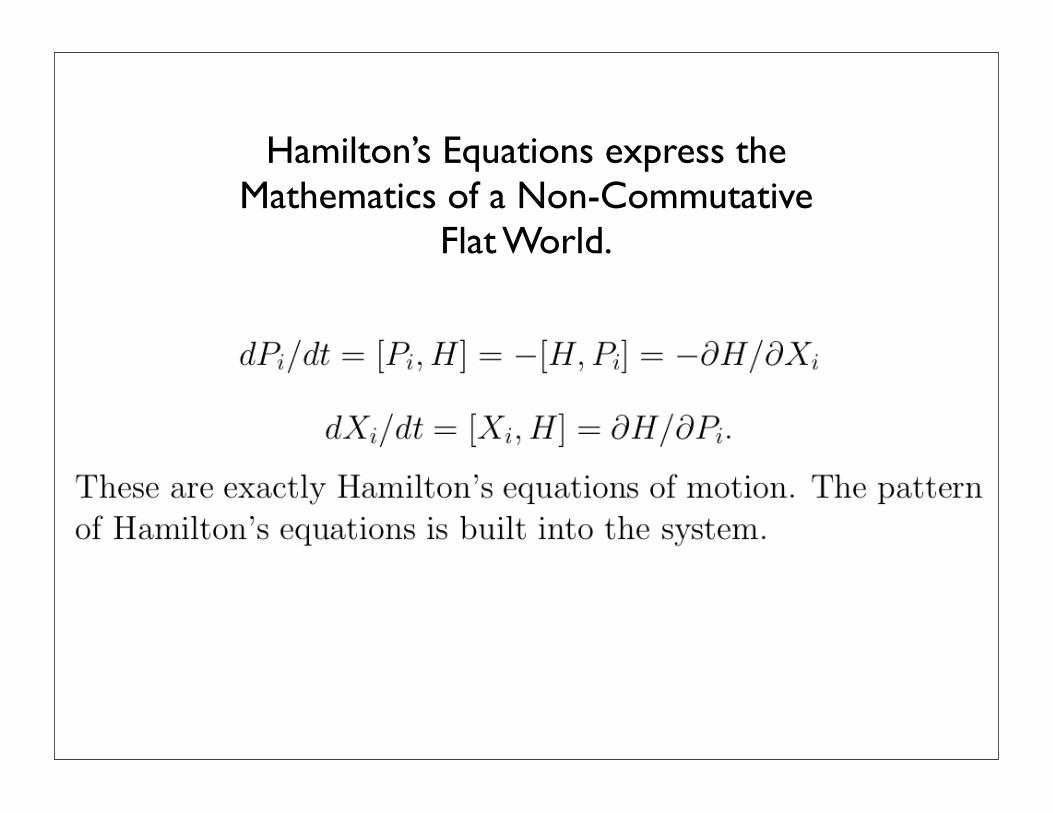
Hamilton’s Equations express the Mathematics of a Non-Commutative
Flat World.

This is the well-known formula for the curvature of a gauge connection.
For the second property, we have
∇fX(Y ) = [Y, PfX ] = [Y, fPX ] = [Y, f ]PX+f [Y, PX ] = 0+f∇X(Y ) = f∇X(Y ).
For the third property, note that
∇X(fY ) = [fY, PX ] = [f, PX ]Y + f [Y, PX ] = X[f ]Y + f∇X(Y ).
This completes the proof.
Definition. We define the curvature as a function R : X ×X ×X −→ A bythe formula
R(X, Y )Z = [∇X ,∇Y ]Z −∇[X,Y ]Z.
Thus for given elements X, Y ∈ X , the curvature operator R(X, Y ) measuresthe non-commutativity of the operators ∇X and ∇Y in relation to the non-commutativity of X and Y. If X and Y commute, then
R(X, Y )Z = [∇X ,∇Y ]Z,
and we are returned to our initial definition of curvature for a collection ofderivations.
5 General Equations of Motion
Given a set of coordinates X1, X2, · · ·Xd and dual coordinates P1, P2, · · ·Pdas in the previous section, a general description of dXi/dt takes the form ofa system of equations
dXi/dt = Gi
where G1, · · · ,Gd is a collection of elements of A. If we choose to write Gi
relative to the flat coordinates via Gi = Pi − Ai (this is a definition of Ai)then the formalism of gauge theory appears naturally. For example, if
∇i(F ) = [F,Gi],
then we have the curvature
[∇i,∇j]F = [Rij, F ]
23

One can explore formulations of discrete physics in non-commutative context.
The context of non-commutative calculus where the derivatives are represented by commutators is directly
related to physics in a new way by this translation of the discrete. This also suggests opening the books again on the
relationship of commutators and quantum theory.

KNOTS AND PHYSICS 9
FIGURE 7. Exchange Identity for Vassiliev Invariants
The upshot of this Lemma is that Vassiliev invariants of type k are intimately involvedwith certain abstract evaluations of graphs with k nodes. In fact, there are restrictions (thefour-term relations) on these evaluations demanded by the topology and it follows from re-sults of Kontsevich [4] that such abstract evaluations actually determine the invariants. Theknot invariants derived from classical Lie algebras are all built from Vassiliev invariants offinite type. All of this is directly related to Witten’s functional integral [41].
In the next few figures we illustrate some of these main points. In Figure 8 we showhow one associates a so-called chord diagram to represent the abstract graph associatedwith an embedded graph. The chord diagram is a circle with arcs connecting those pointson the circle that are welded to form the corresponding graph. In Figure 9 we illustratehow the four-term relation is a consequence of topological invariance. Figure 9 is the mostimportant part of the connection of the topology and the algebra for Vassiliev invariants.
Look closely at this figure. The top of the figure illustrates a simple topological equiv-alence related to the rigid vertex. Two segments (parts of a larger diagram) cross to forma vertex. On the left-hand side of the equality a loop passes under all parts of the crossingsegments. On the right-hand side of the equality the loop passes over all parts of the cross-ing segments. The two figures (left and right) are topologically equivalent as they stand,and if they appear inside any larger diagram that has the same local appearance as thesefigures. The equivalence is obtained by contracting the loop from under the crossing andthen expanding it above the crossing, going from the left part of the equality to the rightpart of the equality. But there is another way to go from the under-crossing diagram to theover-crossing diagram. This second way is given in detail by the four equations that aregrouped in the next part of Figure 9. The first equation begins with our familiar left-sidediagram and subtracts the result of switching a single crossing. The result (since we areevaluating Vassiliev invariants) is the new diagram on the right with the switched crossingreplaced by a node. Thus the diagram on the right has two nodes. We repeat this procedurefour times, each time switching one more crossing and arranging the equations so that thelast equation involves the right-hand diagram where the loop is entirely above the cross-ing. Adding these four equations together yields complete cancellation of the sum of theirleft-sides, and we obtain the boxed equation of diagrams with two nodes each. This is theembedded four-term relation. In the embedded four-term relation we see a central nodeand four neighboring nodes. The neighbors fall into pairs to the left and to the right of the
Knots, Links and Lie AlgebrasVassiliev Invariants
10 LOUIS H. KAUFFMAN
FIGURE 8. Chord Diagrams.
FIGURE 9. The Four Term Relation from Topology
central node. From the embedded four-term relation we go directly to the abstract four-term relation shown directly below it in the chord diagram language. It is a good exerciseto make this translation yourself. The abstract four term relation exhibits neighbor rela-tions among crossings in a direct way with one neighbor difference on the left-hand sideof the equation, and another neighbor difference on the right-hand side of the equation.
Skein Identity
Chord Diagram
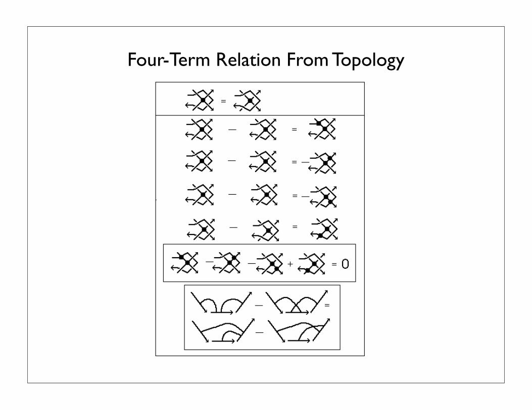
10 LOUIS H. KAUFFMAN
FIGURE 8. Chord Diagrams.
FIGURE 9. The Four Term Relation from Topology
central node. From the embedded four-term relation we go directly to the abstract four-term relation shown directly below it in the chord diagram language. It is a good exerciseto make this translation yourself. The abstract four term relation exhibits neighbor rela-tions among crossings in a direct way with one neighbor difference on the left-hand sideof the equation, and another neighbor difference on the right-hand side of the equation.
Four-Term Relation From Topology
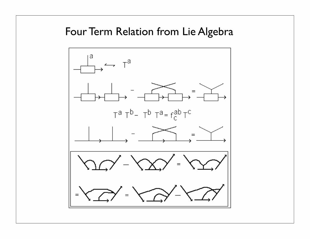
KNOTS AND PHYSICS 11
FIGURE 10. The Four Term Relation from Categorical Lie Algebra.
a b
a b
a b
-a ba
a a
b
b b
c
c ca b
(a b) c
a c (a c) bb c
a (b c)
- =
(a b) c - (a c) b = a (b c)Hence(a b) c + b (a c) = a (b c).
FIGURE 11. The Jacobi Identity.
Four Term Relation from Lie Algebra
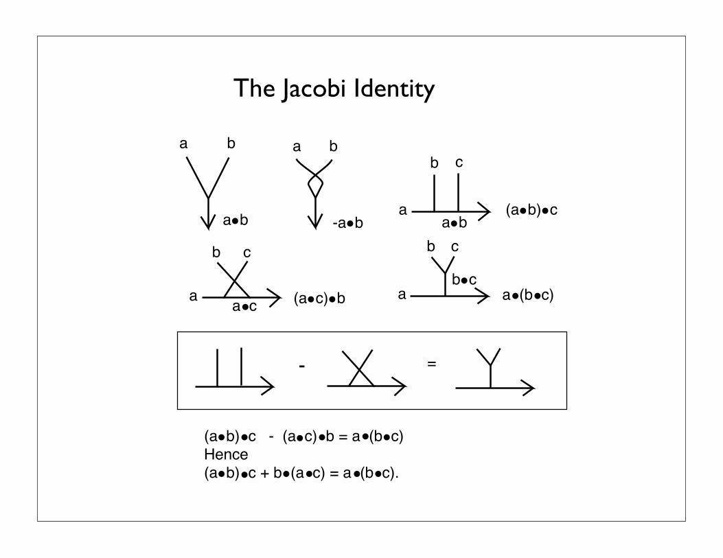
KNOTS AND PHYSICS 11
FIGURE 10. The Four Term Relation from Categorical Lie Algebra.
a b
a b
a b
-a ba
a a
b
b b
c
c ca b
(a b) c
a c (a c) bb c
a (b c)
- =
(a b) c - (a c) b = a (b c)Hence(a b) c + b (a c) = a (b c).
FIGURE 11. The Jacobi Identity.
The Jacobi Identity

12/8/08 6:43 PMRishon Model of Elementary Particles
Page 1 of 3http://jasia.ca/jaydshelton/rishonmodel/
by J. D. Shelton
It has been proposed that the quarks and leptons consist of
more fundamental particles called rishons. The T rishon
may be defined as having mass and charge e/3. The V
rishon is neutral and has little or no mass. The rishons have
spin !, carry color charge, and combine in triplets or
rishon-antirishon pairs. Thus the electron is a TTT, the
neutrino VVV, the down quark TVV, and the up quark TTV.
If the T has somewhat greater color charge than the V, the
down quark would have a net excess of the color carried by
the T. The antiup quark TTV would appear to have a net
deficiency of the color carried by the V, or equivalently, an
excess of anticolor, and behave as an antiparticle. Hence the
TTV would appear to have an excess of color and behave as
a particle, in agreement with observation. The leptons have
no net color. There is no need for hypercolor.
All particle interactions consist of rearrangements of
rishons, or creation or annihilation of rishon-antirishon
pairs. For example, beta-decay occurs when a down quark
changes to an up quark, emitting an electron and neutrino:
TVV --> TTV + TTT + VVV
The massless particle was originally called a neutrino; it was
later defined to be an antineutrino. This model favors the
first choice.
If the binding between rishons is much greater than the
binding between quarks or leptons, then quarks and leptons
could associate without losing their identity, just as atoms
can form molecules. Lepton number is also conserved if the
VVV is assigned a negative lepton number.
The second and third generations of the electron and the
quarks might be formed by adding one or two TT pairs to
the first generation. The second and third generations of the
About the Author
Contact

12/8/08 6:41 PMThe Bilson-Thompson Helon (Braid) Model « Mass
Page 2 of 8http://carlbrannen.wordpress.com/2007/07/17/the-bilson-thompson-helon-braid-model/
background independent models of quantum spacetime that “propagate
coherently as they can be shown to be noiseless subsystems of the microscopic
quantum dynamics”.
Since I play with a similar preon model, I thought I would comment on this
theory from my perspective. I’ve given links to a few of the technical terms, but
this post is not going to make a lot of sense to those not already playing with
particle physics.
In his original paper, Bilson-Thompson called his idea the “Helon Model”. It is
based on an earlier preon model by Harari and Shupe that was called the
“Rishon Model”. See Wikipedia on Rishon model, J. D. Shelton’s short
description, Harari’s original paper (scanned to acrobat), or, if you have Phys.
Lett. B access, Shupe’s original article.
The Rishon Model described the fundamental fermions of the first generation,
that is, the electron and its neutrino, the up quark, and the down quark, (as well
as their antiparticles) as being composites made up of three preons each. Just
like the quarks, the preons com in three colors (or precolors), and the observed
fermions are made up of color singlets in the same manner as the baryons. In
addition to color, the preons also come with electric charges of 1/3 or 0. These
preons are Dirac spinor particles, so they come in four varieties. Such a preon
can have spin up or down, and can be a particle or antiparticle. The neutral
preons are called V and the charged ones are called T.
With these particles, the structure of a generation of elementary fermions can be
constructed by assuming only two requirements are necessary to produce a
bound state: (1) It must be a precolor singlet. (2) It must be composed purely of
3 preons or 3 anti preons. The resulting particle content is as follows (for the
first generation):
TTT positron
TTV up quark, red
TVT up quark, green
VTT up quark, blue
VVT anti down quark, red
VTV anti down quark, green
TVV anti down quark, blue
VVV electron neutrino
In the above, note that while the three preons included are all particles, the
resulting fermions are half particles (the up quark and electron neutrino), and
half anti-particles (the down quark and positron). If you change the Ts and Vs to
antiparticles, you get the down quark, electron, anti up quark, and anti electron
neutrino.
Bilson-Thomposon’s Changes to the Rishon Model
Preon models are supposed to use the traditional point particles of quantum
field theory. Bilson-Thompson’s model is not of point particles, but instead is a
topological model. He wrote:
The reader should note the subtle yet important distinction that this is not a
preon model per se, based upon point-like particles, but rather a preon-
inspired model, which may be realised as a topological feature of some more
November 2008
October 2008
September 2008
August 2008
July 2008
June 2008
May 2008
April 2008
March 2008
February 2008
January 2008
December 2007
November 2007
October 2007
September 2007
August 2007
July 2007
June 2007
May 2007
April 2007
February 2007
August 2006
Log in
Entries RSS
Comments RSS
WordPress.com
Meta
A Babe in the Universe
A Quantum Diaries Survivor
Al Fin
Angry Physics
Arcadian Functor
Boudicca’s Voice
Built On Facts
Direction of Grace
Geometric Algebra Update Blog
God Plays Dice
Iowa Hawk
Mahndisa S. Rigmaiden
Marco Frasca
Moses Lake
Nanoscale Views
Pandora
Parkway Rest Stop
Resonances
Blogroll
arX
iv:h
ep-p
h/0
50
32
13
v2
2
7 O
ct 2
00
6
ADP-05-05/T615
A topological model of composite preons
Sundance O. Bilson-Thompson∗
Centre for the Subatomic Structure of Matter, Department of Physics,University of Adelaide, Adelaide SA 5005, Australia
(Dated: February 2, 2008)
We describe a simple model, based on the preon model of Shupe and Harari, in which the bindingof preons is represented topologically. We then demonstrate a direct correspondence between thismodel and much of the known phenomenology of the Standard Model. In particular we identify thesubstructure of quarks, leptons and gauge bosons with elements of the braid group B3. Importantly,the preonic objects of this model require fewer assumed properties than in the Shupe/Harari model,yet more emergent quantities, such as helicity, hypercharge, and so on, are found. Simple topologicalprocesses are identified with electroweak interactions and conservation laws. The objects which playthe role of preons in this model may occur as topological structures in a more comprehensive theory,and may themselves be viewed as composite, being formed of truly fundamental sub-components,representing exactly two levels of substructure within quarks and leptons.
PACS numbers: 12.60.Rc, 12.10.Dm
I. INTRODUCTION
The Standard Model (SM) provides an extremely suc-cesful and simple means of classifying and understand-ing the physical processes which fill the Universe. How-ever the existence of many seemingly arbitrary featureshints at a more fundamental physical theory from whichthe SM arises. Considering the successful series of ideasleading through molecules, to atoms, nuclei, nucleons,and quarks, it was perhaps inevitable that a model basedon compositeness of quarks and leptons would be devel-oped. The first such was proposed by Pati and Salam [1]in 1974, however it lacked any real explanatory power.Pati and Salam gave the name preons to their hypo-thetical constituent particles, and this name was grad-ually adopted to refer to the sub-quark/sub-lepton par-ticles of any model. Other notable preon models weredeveloped by several authors (e.g. [2]), but it is the so-called Rishon Model, proposed simultaneously by Harariand Shupe [3, 4] which will be of most interest to ushere. In Harari’s more commonly quoted terminology,this model involves just two kinds of ‘rishons’, one car-rying an electric charge of +e/3 where −e is the chargeon the electron, the other neutral. The rishons combineinto triplets, with the two “three-of-a-kind” triplets be-ing interpreted as the νe and e+, and the permutations oftriplets with an “odd-man-out” being interpreted as thedifferent colours of quarks. Equivalent combinations canbe formed from the anti-rishons to create the remainingfermions and anti-fermions, such as the e− and νe. Cer-tain combinations of rishons and anti-rishons were alsosuggested to correspond with gauge bosons.The rishon model accounted for many aspects of the SM,including the precise ratios of lepton and quark electriccharges, and the correspondence between fractional elec-
∗Electronic address: [email protected]
tric charge and colour charge. Unfortunately, as origi-nally proposed it also had several problems, including thelack of a dynamical framework, and the lack of an expla-nation as to why the ordering of rishons within tripletsshould matter. A charge called “hypercolour” was pro-posed to solve these problems [5]. The introduction ofhypercolour implied the existence of “hypergluons” andsome QCD-like confinement mechanism for the rishons.Hence, the simplicity of the original model was reduced,and many of the fundamental questions about particlesand interactions were simply moved to the realm of ris-hons, yielding little obvious advantage over the SM. Fur-thermore preon models were never able to adequately an-swer several fundamental questions, such as how preonsconfined at all length scales experimentally probed canform very light composites (see e.g. [6] for an attempt toaddress this issue).This article presents an idea based on the original rishonmodel (without hypercolour), which we call the HelonModel. The reader should note the subtle yet importantdistinction that this is not a preon model per se, basedupon point-like particles, but rather a preon-inspiredmodel, which may be realised as a topological featureof some more comprehensive theory. For this reason wedo not believe that the objections levelled at the rishonmodel and other preon models should be assumed, a pri-ori, to be relevant to the helon model. A thorough in-vestigation of such issues will be undertaken in subse-quent work, however they are beyond the scope of thecurrent article. Here we simply present a pedagogical in-troduction to the helon model, and describe how variousfeatures of the standard model emerge from it.
II. THE HELON MODEL
Let us now introduce our topologically-based toymodel of quarks, leptons, and gauge bosons. It is conve-nient to represent the most fundamental objects in this

arX
iv:h
ep-p
h/0
503213v2 27 O
ct 2
006
ADP-05-05/T615
A topological model of composite preons
Sundance O. Bilson-Thompson∗
Centre for the Subatomic Structure of Matter, Department of Physics,University of Adelaide, Adelaide SA 5005, Australia
(Dated: February 2, 2008)
We describe a simple model, based on the preon model of Shupe and Harari, in which the bindingof preons is represented topologically. We then demonstrate a direct correspondence between thismodel and much of the known phenomenology of the Standard Model. In particular we identify thesubstructure of quarks, leptons and gauge bosons with elements of the braid group B3. Importantly,the preonic objects of this model require fewer assumed properties than in the Shupe/Harari model,yet more emergent quantities, such as helicity, hypercharge, and so on, are found. Simple topologicalprocesses are identified with electroweak interactions and conservation laws. The objects which playthe role of preons in this model may occur as topological structures in a more comprehensive theory,and may themselves be viewed as composite, being formed of truly fundamental sub-components,representing exactly two levels of substructure within quarks and leptons.
PACS numbers: 12.60.Rc, 12.10.Dm
I. INTRODUCTION
The Standard Model (SM) provides an extremely suc-cesful and simple means of classifying and understand-ing the physical processes which fill the Universe. How-ever the existence of many seemingly arbitrary featureshints at a more fundamental physical theory from whichthe SM arises. Considering the successful series of ideasleading through molecules, to atoms, nuclei, nucleons,and quarks, it was perhaps inevitable that a model basedon compositeness of quarks and leptons would be devel-oped. The first such was proposed by Pati and Salam [1]in 1974, however it lacked any real explanatory power.Pati and Salam gave the name preons to their hypo-thetical constituent particles, and this name was grad-ually adopted to refer to the sub-quark/sub-lepton par-ticles of any model. Other notable preon models weredeveloped by several authors (e.g. [2]), but it is the so-called Rishon Model, proposed simultaneously by Harariand Shupe [3, 4] which will be of most interest to ushere. In Harari’s more commonly quoted terminology,this model involves just two kinds of ‘rishons’, one car-rying an electric charge of +e/3 where −e is the chargeon the electron, the other neutral. The rishons combineinto triplets, with the two “three-of-a-kind” triplets be-ing interpreted as the νe and e+, and the permutations oftriplets with an “odd-man-out” being interpreted as thedifferent colours of quarks. Equivalent combinations canbe formed from the anti-rishons to create the remainingfermions and anti-fermions, such as the e− and νe. Cer-tain combinations of rishons and anti-rishons were alsosuggested to correspond with gauge bosons.The rishon model accounted for many aspects of the SM,including the precise ratios of lepton and quark electriccharges, and the correspondence between fractional elec-
∗Electronic address: [email protected]
tric charge and colour charge. Unfortunately, as origi-nally proposed it also had several problems, including thelack of a dynamical framework, and the lack of an expla-nation as to why the ordering of rishons within tripletsshould matter. A charge called “hypercolour” was pro-posed to solve these problems [5]. The introduction ofhypercolour implied the existence of “hypergluons” andsome QCD-like confinement mechanism for the rishons.Hence, the simplicity of the original model was reduced,and many of the fundamental questions about particlesand interactions were simply moved to the realm of ris-hons, yielding little obvious advantage over the SM. Fur-thermore preon models were never able to adequately an-swer several fundamental questions, such as how preonsconfined at all length scales experimentally probed canform very light composites (see e.g. [6] for an attempt toaddress this issue).This article presents an idea based on the original rishonmodel (without hypercolour), which we call the HelonModel. The reader should note the subtle yet importantdistinction that this is not a preon model per se, basedupon point-like particles, but rather a preon-inspiredmodel, which may be realised as a topological featureof some more comprehensive theory. For this reason wedo not believe that the objections levelled at the rishonmodel and other preon models should be assumed, a pri-ori, to be relevant to the helon model. A thorough in-vestigation of such issues will be undertaken in subse-quent work, however they are beyond the scope of thecurrent article. Here we simply present a pedagogical in-troduction to the helon model, and describe how variousfeatures of the standard model emerge from it.
II. THE HELON MODEL
Let us now introduce our topologically-based toymodel of quarks, leptons, and gauge bosons. It is conve-nient to represent the most fundamental objects in this
2
model by twists through ±π in a ribbon. For conveniencelet us denote a twist through π as a “dum”, and a twistthrough −π as a “dee” (U and E for short, after Tweedle-dum and Tweedle-dee [7]). Generically we refer to suchtwists by the somewhat whimsical name “tweedles”[8].We hope to deduce the properties of quarks and leptonsand their interactions from the behaviour of their con-stituent tweedles, and to do so we shall employ a set ofassumptions that govern their behaviour:1) Unordered pairing: Tweedles combine in pairs, sothat their total twist is 0 modulo 2π, and the orderingof tweedles within a pair is unimportant. The three pos-sible combinations of UU , EE, and UE ≡ EU can berepresented as ribbons bearing twists through the angles+2π, −2π, and 0 respectively. A twist through ±2π isinterpreted as an electric charge of ±e/3. We shall referto such pairs of tweedles as helons (evoking their helicalstructure) and denote the three types of helons by H+,H−, and H0.2) Helons bind into triplets: Helons are bound intotriplets by a mechanism which we represent as the topsof each strand being connected to each other, and the bot-toms of each strand being similarly connected. A tripletof helons may split in half, in which case a new connectionforms at the top or bottom of each resulting triplet. Thereverse process may also occur when two triplets mergeto form one triplet, in which case the connection at thetop of one triplet and the bottom of the other triplet “an-nihilate” each other.The arrangement of three helons joined at the top andbottom is equivalent to two parallel disks connected bya triplet of strands. In the simplest case, such an ar-rangement is invariant under rotations through anglesof 2π/3, making it impossible to distinguish the strandswithout arbitrarily labelling or colouring them. Howeverwe can envisage the three strands crossing over or undereach other to form a braid. The three strands can thenbe distinguished by their relative crossings. We will ar-gue below that braided triplets represent fermions, whileunbraided triplets provide the simplest way to representgauge bosons.3) No charge mixing: When constructing braidedtriplets, we will not allow H+ and H− helons in the sametriplet. H+ and H0 mixing, and H− and H0 mixing areallowed.4) Integer charge: All unbraided triplets must carryinteger electric charge.Assumption 1) is unique to the helon model, as it reflectsthe composite nature of helons, however assumptions 2),3) and 4) are merely restatements in a different context ofassumptions that Shupe and Harari made in their work.We will require one further assumption, however it willbe left until later, as it can be better understood in theproper context.In terms of the number of fundamental objects, the helonmodel is more economical than even the rishon model, al-beit at the cost of allowing helons to be composite. Thisseems a reasonable price to pay, as the tweedles are ex-
tremely simple, being defined by only a single property(i.e. whether they twist through +π or −π). This maybe interpreted as representing exactly two levels of sub-structure within quarks and leptons.The helon model also improves on the original rishonmodel by explaining why the ordering of helons (whichare analogous to rishons) should matter. There are threepermutations of any triplet with a single “odd-man-out”.Without braiding we cannot distinguish these permuta-tions, by the rotational invariance argument above. How-ever, if we allow braiding, the strands (and hence per-mutations) become distinct, in general. We may asso-ciate these permutations with the three colour charges ofQCD, just as was done in the rishon model, and write thehelons in ordered triplets for convenience. The possiblecombinations and their equivalent quarks are as follows(subscripts denote colour):
H+H+H0 (uB) H+H0H+ (uG) H0H+H+ (uR)H0H0H+ (dB) H0H+H0 (dG) H+H0H0 (dR)H−H−H0 (uB) H−H0H− (uG) H0H−H− (uR)H0H0H− (dB) H0H−H0 (dG) H−H0H0 (dR).
while the leptons are:
H+H+H+ (e+) H0H0H0 (νe) H−H−H− (e−)
Note that in this scheme we have created neutrinos, butnot anti-neutrinos. This has occurred because the H0
helon is its own anti-particle. This apparent problem willbe turned to our advantage in Section III. Note also thatwe have not ascribed any of the usual quantum numbers(such as mass or spin [13]) to the helons. It is our expec-tation that spin, mass, hypercharge and other quantitiesemerge dynamically, just like electric charge, as we ar-range helons into more complex patterns.It is interesting to note that three helons seems to bethe minimum number from which a stable, non-trivialstructure can be formed. By stable, we mean that aphysical representation of a braid on three strands (e.g.made from strips of fabric) cannot in general be smoothlydeformed into a simpler structure. By contrast, such aphysical model with only two strands can always be un-twisted.
III. PHENOMENOLOGY OF THE HELON
MODEL
A braid on n strands is said to be an element of thebraid group Bn. Given any element of Bn, it is also pos-sible to create a corresponding anti-braid, which is thetop-to-bottom mirror image of that braid, and is also anelement of Bn (it is therefore merely a matter of conven-tion what we call a braid or an anti-braid). If we jointhe strands of a braid with those of its top-to-bottommirror image (i.e. we take the braid product [9]) we ob-tain a structure which can be deformed into the trivialbraid. Conversely, if the strands of a trivial braid arecrossed so as to form a braid, an anti-braid must also be

3
FIG. 1: The fermions formed by adding zero, one, two orthree charges to a neutral braid. Charged fermions come intwo handedness states each, while ν and ν come in only oneeach. (3) denotes that there are three possible permutations,identified as the quark colours. The bands at top and bottomrepresent the binding of helons.
formed. Thus if we assign a quantity β = +1 to braidsand β = −1 to anti-braids, NB =
!
β is conserved insplitting and joining operations (where the sum is takenover all braids and anti-braids present). These proper-ties are reminiscent of the relationship between particlesand anti-particles, and so it is natural to use the top-to-bottom mirroring of braids as a model for particle–anti-particle interchange, or C inversion. In addition, givenany element of Bn, its left-to-right mirror image maybe formed. We will call these the left-handed and right-handed forms of a braid. It seems natural to equate thesewith particles and anti-particles having positive and neg-ative helicity. From the discussion above, all fermionsand their anti-particles are represented by braids whichare elements of B3.Let us construct the first-generation fermions with pos-itive charge as shown on the right of Figure 1 (we areusing a basic braid, like that used to plait hair, for illus-trative purposes, however an arbitrary number of cross-ings is possible). This yields the positron, up quark,anti-down quark, and anti-neutrino. Now let us con-struct the negatively-charged fermions by taking thetop-to-bottom mirror images of the positively chargedfermions. We have constructed the positively chargedfermions by adding positive charges (dees) to a right-handed braid, and their anti-particles by adding negativecharges (dums) to a left-handed anti-braid. This deci-sion was of course completely arbitrary. We can also adddees to a left-handed braid and dums to a right-handedanti-braid. If we do this, we create all the possible charge-carrying braids in two different handedness states exactlyonce, but following the same procedure for the unchargedbraids (i.e. neutrinos and anti-neutrinos) would mean du-plicating them, since this second pair of neutral leptons isidentical to the first pair, rotated through ±π. In otherwords, to avoid double-counting we can only constructthe (anti-)neutrino in a (right-)left-handed form, whileall the other fermions come in both left- and right-handedforms. This pleasing result is a direct consequence of thefact that we construct the neutrino and anti-neutrino
FIG. 2: A representation of the decay µ → νµ+e−+νe, show-ing how the substructure of fermions and bosons demandsthat charged leptons decay to neutrinos of the same genera-tion.
from the same sub-components (by contrast the rishonmodel used neutral rishons for the νe and neutral anti-rishons for the νe).If we perform C and P operations on any braid (excepta ν or ν, on which we cannot perform P) we obtain thebraid diagonally opposite it in Figure 1. We may define afurther operation which consists of rotating a braid clock-wise or anti-clockwise through π, and reversing the signof all charges. This operation will be called T, and wenote that performing C, P, and T in any order on a braidleaves that braid unchanged.Having constructed the quarks and leptons, we now turnour attention to their interactions via the electroweakand colour forces.The Electroweak Interaction We shall begin by con-structing the bosons of the electroweak interaction, γ,W+, W−, and Z0. The W+ and W− may be regardedas a triplet of H+s and a triplet of H−s respectively. Wecan create neutral bosons from a triplet of similar helonsin two ways. One is as a triplet of untwisted helons, theother as a triplet of “counter-twisted” helons (that is,each helon carries explicit left-handed and right-handedtwists). We shall claim that the former is the photon,the latter is the Z0 (we may also speculate that deform-ing an untwisted helon into a counter-twisted helon, orvice-versa, accounts for the Weinberg mixing between theZ0 and the photon [14]). What sets bosons apart fromfermions (i.e. so that a γ is distinct from a neutrino,and a W± is distinct from an e±) is that the strand per-mutation induced by the braid that forms a boson is theidentity permutation. The simplest braid that fulfills thiscriterion is the trivial braid, as in Fig. 3.All interactions between helons can be viewed as cuttingor joining operations, in which twists (tweedles) may beexchanged between helons. These operations define ba-sic vertices for helon interactions. By combining threeof these basic helon vertices in parallel we construct thebasic vertices of the electroweak interaction (Figure 4).Crossing symmetries of the helon vertices automaticallyimply the usual crossing symmetries for the electroweakvertices.We can represent higher generation fermions by allow-
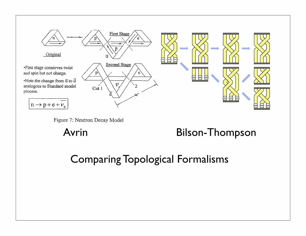
Comparing Topological Formalisms
Avrin Bilson-Thompson

3
FIG. 1: The fermions formed by adding zero, one, two orthree charges to a neutral braid. Charged fermions come intwo handedness states each, while ν and ν come in only oneeach. (3) denotes that there are three possible permutations,identified as the quark colours. The bands at top and bottomrepresent the binding of helons.
formed. Thus if we assign a quantity β = +1 to braidsand β = −1 to anti-braids, NB =
!
β is conserved insplitting and joining operations (where the sum is takenover all braids and anti-braids present). These proper-ties are reminiscent of the relationship between particlesand anti-particles, and so it is natural to use the top-to-bottom mirroring of braids as a model for particle–anti-particle interchange, or C inversion. In addition, givenany element of Bn, its left-to-right mirror image maybe formed. We will call these the left-handed and right-handed forms of a braid. It seems natural to equate thesewith particles and anti-particles having positive and neg-ative helicity. From the discussion above, all fermionsand their anti-particles are represented by braids whichare elements of B3.Let us construct the first-generation fermions with pos-itive charge as shown on the right of Figure 1 (we areusing a basic braid, like that used to plait hair, for illus-trative purposes, however an arbitrary number of cross-ings is possible). This yields the positron, up quark,anti-down quark, and anti-neutrino. Now let us con-struct the negatively-charged fermions by taking thetop-to-bottom mirror images of the positively chargedfermions. We have constructed the positively chargedfermions by adding positive charges (dees) to a right-handed braid, and their anti-particles by adding negativecharges (dums) to a left-handed anti-braid. This deci-sion was of course completely arbitrary. We can also adddees to a left-handed braid and dums to a right-handedanti-braid. If we do this, we create all the possible charge-carrying braids in two different handedness states exactlyonce, but following the same procedure for the unchargedbraids (i.e. neutrinos and anti-neutrinos) would mean du-plicating them, since this second pair of neutral leptons isidentical to the first pair, rotated through ±π. In otherwords, to avoid double-counting we can only constructthe (anti-)neutrino in a (right-)left-handed form, whileall the other fermions come in both left- and right-handedforms. This pleasing result is a direct consequence of thefact that we construct the neutrino and anti-neutrino
FIG. 2: A representation of the decay µ → νµ+e−+νe, show-ing how the substructure of fermions and bosons demandsthat charged leptons decay to neutrinos of the same genera-tion.
from the same sub-components (by contrast the rishonmodel used neutral rishons for the νe and neutral anti-rishons for the νe).If we perform C and P operations on any braid (excepta ν or ν, on which we cannot perform P) we obtain thebraid diagonally opposite it in Figure 1. We may define afurther operation which consists of rotating a braid clock-wise or anti-clockwise through π, and reversing the signof all charges. This operation will be called T, and wenote that performing C, P, and T in any order on a braidleaves that braid unchanged.Having constructed the quarks and leptons, we now turnour attention to their interactions via the electroweakand colour forces.The Electroweak Interaction We shall begin by con-structing the bosons of the electroweak interaction, γ,W+, W−, and Z0. The W+ and W− may be regardedas a triplet of H+s and a triplet of H−s respectively. Wecan create neutral bosons from a triplet of similar helonsin two ways. One is as a triplet of untwisted helons, theother as a triplet of “counter-twisted” helons (that is,each helon carries explicit left-handed and right-handedtwists). We shall claim that the former is the photon,the latter is the Z0 (we may also speculate that deform-ing an untwisted helon into a counter-twisted helon, orvice-versa, accounts for the Weinberg mixing between theZ0 and the photon [14]). What sets bosons apart fromfermions (i.e. so that a γ is distinct from a neutrino,and a W± is distinct from an e±) is that the strand per-mutation induced by the braid that forms a boson is theidentity permutation. The simplest braid that fulfills thiscriterion is the trivial braid, as in Fig. 3.All interactions between helons can be viewed as cuttingor joining operations, in which twists (tweedles) may beexchanged between helons. These operations define ba-sic vertices for helon interactions. By combining threeof these basic helon vertices in parallel we construct thebasic vertices of the electroweak interaction (Figure 4).Crossing symmetries of the helon vertices automaticallyimply the usual crossing symmetries for the electroweakvertices.We can represent higher generation fermions by allow-

4
FIG. 3: The bosons of the electroweak interaction. Noticethat the Z0 and the photon can deform into each other.
ing the three helons to cross in more complicated pat-terns. Thus all fermions may be viewed as a basic neu-trino “framework” to which electric charges are added,and the structure of this framework determines to whichgeneration a given fermion belongs. If, say, a muon emitscharge in the form of a W− boson, the emission of this(trivially braided) boson does not affect the fermion’sbraiding structure. Therefore the muon loses charge butdoes not change generation, and must transform into amuon-neutrino. Likewise, tau-neutrinos may only trans-form into tau particles and electron-neutrinos may onlytransform into electrons. A similar argument applies toquarks, although the mechanism by which the Cabibboangles become non-zero is not immediately apparent. No-tice that since W± bosons carry three like charges, suchprocesses will change quark flavour but not colour.The Colour Interaction We have thus far describedelectroweak interactions as splitting and joining opera-tions on braids. We may similarly represent colour in-teractions physically, this time as the formation of a“pancake stack” of braids. Each set of strands that lieone-above-the-other can be regarded as a “super-strand”,with a total charge equal to the sum of the charges oneach of its component strands. If we represent braids aspermutation matrices, with each non-zero component be-ing a helon, we can easily represent the colour interactionbetween fermions as the sum of the corresponding matri-ces. For instance a red up quark, and an anti-red anti-upcombining to form a neutral pion could be represented as
⎡
⎣
0 0 H0
H+ 0 00 H+ 0
⎤
⎦ +
⎡
⎣
0 0 H0
H− 0 00 H− 0
⎤
⎦
=
⎡
⎣
0 0 H0 + H0
H+ + H− 0 00 H+ + H− 0
⎤
⎦ (1)
where the sum of two helons on the right-hand-side de-notes a super-strand composed of a pair of helons. In thiscase all three super-strands have zero net charge. In thisway hadrons can be regarded as a kind of superpositionof quarks. We can now introduce our last assumption.5) Charge equality:When two or more braids arestacked, they must combine to produce the same totalcharge on all three super-strands.It is obvious that leptons trivially fulfill this criterion,
FIG. 4: The charge transferring vertex (TV) and the po-larising vertex (PV) are basic helon vertices from which theelectroweak basic vertices can be formed.
and will therefore not partake of the colour interaction.The reader may verify that quarks will naturally formgroupings with integer electric charge, which are colour-neutral, for example three quarks forming a proton:
dB + uR + uG =
⎡
⎣
0 0 H0
H0 0 00 H− 0
⎤
⎦
+
⎡
⎣
0 0 H0
H+ 0 00 H+ 0
⎤
⎦ +
⎡
⎣
0 0 H+
H0 0 00 H+ 0
⎤
⎦ . (2)
In QCD there are eight gluons. Two of these are super-positions of like colour/anti-colour states, which we mayvisualise as triplets with some untwisted strands, andsome counter-twisted strands (strands with explicit pos-itive and negative twist, as per the description of the Z0,above). The remaining six are “pure” unlike colour/anti-colour pairings, which we can visualise as the six permu-tations of one H+, one H0, and one H−.Hypercharge Recall that we assigned β = +1 to thebraids on the top row of Figure 1, and β = −1 to thebraids on the bottom row. This effectively distinguishesbetween fermions with a net positive and net negativecharge. To distinguish between quarks and leptons thenumber of odd-men-out within any triplet, divided bythe number of helons within a triplet suggests itself asa useful quantity (taking a value of 0 for leptons and1/3 for quarks). However this quantity does not distin-guish between a particle and its anti-particle. To rectifythis shortcoming we will define a new quantity, given byone-third the number of “more positive” helons, minusone-third the number of “less positive” helons. We shalldenote this quantity by the symbol Ω. To clarify, H+
helons are considered “more positive” than H0 helons,which are “more positive” than H− helons. If N(H+) isthe number of H+ helons, N(H0) the number of H0s andN(H−) the number of H−s within a triplet, and remem-bering that H+ and H− helons never occur within thesame braided triplet, we may write
Ω = β
(
1
3N(H+) +
1
3N(H−) −
1
3N(H0)
)
. (3)

2
model by twists through ±π in a ribbon. For conveniencelet us denote a twist through π as a “dum”, and a twistthrough −π as a “dee” (U and E for short, after Tweedle-dum and Tweedle-dee [7]). Generically we refer to suchtwists by the somewhat whimsical name “tweedles”[8].We hope to deduce the properties of quarks and leptonsand their interactions from the behaviour of their con-stituent tweedles, and to do so we shall employ a set ofassumptions that govern their behaviour:1) Unordered pairing: Tweedles combine in pairs, sothat their total twist is 0 modulo 2π, and the orderingof tweedles within a pair is unimportant. The three pos-sible combinations of UU , EE, and UE ≡ EU can berepresented as ribbons bearing twists through the angles+2π, −2π, and 0 respectively. A twist through ±2π isinterpreted as an electric charge of ±e/3. We shall referto such pairs of tweedles as helons (evoking their helicalstructure) and denote the three types of helons by H+,H−, and H0.2) Helons bind into triplets: Helons are bound intotriplets by a mechanism which we represent as the topsof each strand being connected to each other, and the bot-toms of each strand being similarly connected. A tripletof helons may split in half, in which case a new connectionforms at the top or bottom of each resulting triplet. Thereverse process may also occur when two triplets mergeto form one triplet, in which case the connection at thetop of one triplet and the bottom of the other triplet “an-nihilate” each other.The arrangement of three helons joined at the top andbottom is equivalent to two parallel disks connected bya triplet of strands. In the simplest case, such an ar-rangement is invariant under rotations through anglesof 2π/3, making it impossible to distinguish the strandswithout arbitrarily labelling or colouring them. Howeverwe can envisage the three strands crossing over or undereach other to form a braid. The three strands can thenbe distinguished by their relative crossings. We will ar-gue below that braided triplets represent fermions, whileunbraided triplets provide the simplest way to representgauge bosons.3) No charge mixing: When constructing braidedtriplets, we will not allow H+ and H− helons in the sametriplet. H+ and H0 mixing, and H− and H0 mixing areallowed.4) Integer charge: All unbraided triplets must carryinteger electric charge.Assumption 1) is unique to the helon model, as it reflectsthe composite nature of helons, however assumptions 2),3) and 4) are merely restatements in a different context ofassumptions that Shupe and Harari made in their work.We will require one further assumption, however it willbe left until later, as it can be better understood in theproper context.In terms of the number of fundamental objects, the helonmodel is more economical than even the rishon model, al-beit at the cost of allowing helons to be composite. Thisseems a reasonable price to pay, as the tweedles are ex-
tremely simple, being defined by only a single property(i.e. whether they twist through +π or −π). This maybe interpreted as representing exactly two levels of sub-structure within quarks and leptons.The helon model also improves on the original rishonmodel by explaining why the ordering of helons (whichare analogous to rishons) should matter. There are threepermutations of any triplet with a single “odd-man-out”.Without braiding we cannot distinguish these permuta-tions, by the rotational invariance argument above. How-ever, if we allow braiding, the strands (and hence per-mutations) become distinct, in general. We may asso-ciate these permutations with the three colour charges ofQCD, just as was done in the rishon model, and write thehelons in ordered triplets for convenience. The possiblecombinations and their equivalent quarks are as follows(subscripts denote colour):
H+H+H0 (uB) H+H0H+ (uG) H0H+H+ (uR)H0H0H+ (dB) H0H+H0 (dG) H+H0H0 (dR)H−H−H0 (uB) H−H0H− (uG) H0H−H− (uR)H0H0H− (dB) H0H−H0 (dG) H−H0H0 (dR).
while the leptons are:
H+H+H+ (e+) H0H0H0 (νe) H−H−H− (e−)
Note that in this scheme we have created neutrinos, butnot anti-neutrinos. This has occurred because the H0
helon is its own anti-particle. This apparent problem willbe turned to our advantage in Section III. Note also thatwe have not ascribed any of the usual quantum numbers(such as mass or spin [13]) to the helons. It is our expec-tation that spin, mass, hypercharge and other quantitiesemerge dynamically, just like electric charge, as we ar-range helons into more complex patterns.It is interesting to note that three helons seems to bethe minimum number from which a stable, non-trivialstructure can be formed. By stable, we mean that aphysical representation of a braid on three strands (e.g.made from strips of fabric) cannot in general be smoothlydeformed into a simpler structure. By contrast, such aphysical model with only two strands can always be un-twisted.
III. PHENOMENOLOGY OF THE HELON
MODEL
A braid on n strands is said to be an element of thebraid group Bn. Given any element of Bn, it is also pos-sible to create a corresponding anti-braid, which is thetop-to-bottom mirror image of that braid, and is also anelement of Bn (it is therefore merely a matter of conven-tion what we call a braid or an anti-braid). If we jointhe strands of a braid with those of its top-to-bottommirror image (i.e. we take the braid product [9]) we ob-tain a structure which can be deformed into the trivialbraid. Conversely, if the strands of a trivial braid arecrossed so as to form a braid, an anti-braid must also be
The Topology/Stability of the Fabric
Can we imagine these “particles” as bitsof surface interacting in a
“superficial spin foam”.
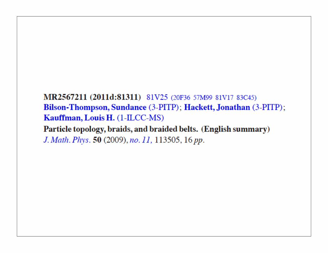
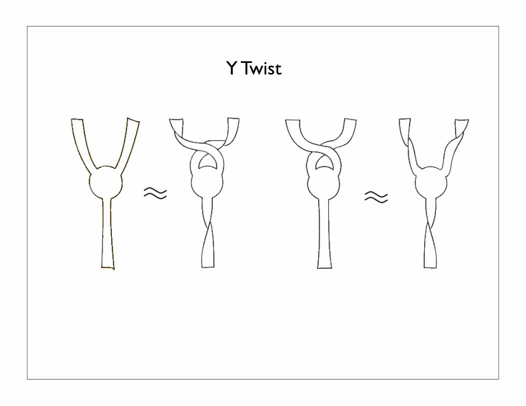
Figure 3: Turning over a node induces crossings and twists in the “legs” ofthat node (left). A trinion flip may be used to eliminate crossing while creatingtwists (right).
consist of n ribbons connecting one set of n points with a common z-coordinate,to another set of n points also with a common z-coordinate, as described above.In braided belts the sets of n points at both ends of the ribbon strands arereplaced by disks, or framed nodes. The union of the strands and disks is aclosed surface. The disks are thus nodes with n “legs” emerging from them, eachleg being the terminus of a ribbon strand. We furthermore relax the conditionthat strands may not “loop back” on themselves. The ability to deform thebraided belt by flipping the node at one end over (eectively feeding it throughthe strands), in order to undo crossings and hence simplify the braid structureof the belt, is essential to the results we will discuss below.
On the left of Fig. 3 we illustrate a Y-shaped ribbon - that is, a node withthree ribbons or “legs” attached to it. Such a triple of ribbons meeting at anode has previously been referred to as a “trinion” [2], and we shall adopt thisterminology. A trinion may be converted into a structure with both crossingsand twists, by keeping the ends fixed and flipping over the node in the middle,as illustrated in Fig. 3 (we shall refer to this process of flipping over a nodewhile keeping the ends of the legs fixed as a “trinion flip”, or “trip” for short).Conversely, on the right of Fig. 3 we show how a trinion with untwisted ribbons,but whose upper ribbons are crossed, can be converted into a trinion withuncrossed ribbons and oppositely-directed half-twists in the upper and lowerribbons by performing an appropriate trinion flip (in the illustration, a negativehalf-twist in the lower ribbon of the trinion and positive half-twists in the upperribbons). In Fig. 4, we show the same process performed on a trinion whose(crossed) upper ribbons have been bent downwards to lie besides and to the leftof the (initially) lower ribbon. This configuration is nothing other than a framed3-braid corresponding to the generator 1 (with the extra detail that the topsof all three strands are joined at a node). Keeping the ends of the ribbons fixedas before and flipping over the node so as to remove the crossings now resultsin three unbraided (i.e. trivially braided) strands, with a positive half-twist on
5
Y Twist

~~
~~Twist1
~~~~Twist2
~~
~~~~
-1/2 -1/2 -1/2 -1/2
+1/2
+1/2
+1/2 +1/2 +1/2 +1/2
-1/2
-1/2
0
0 0 0 0 0
0 0
0
0 0 0
Figure 2: The Twist
~~
Figure 3: The Twist on a closed 3-Belt
4
Basic Twists

~~
~~Twist1
~~~~Twist2
~~
~~~~
-1/2 -1/2 -1/2 -1/2
+1/2
+1/2
+1/2 +1/2 +1/2 +1/2
-1/2
-1/2
0
0 0 0 0 0
0 0
0
0 0 0
Figure 2: The Twist
~~
Figure 3: The Twist on a closed 3-Belt
4

~~~~
Figure 4: Braiding a Belt
braid B. They will get permuted in the process, according to the permutation(B) associated with the braid B. Thus
[r, s, t]B[r, s, t]B = [r, s, t][r, s, t](B)BB
where [r, s, t][x, y, z] = [r + x, s + y, t + z] and BB denotes the usual product ofbraid words.
For example,
[r, s, t]1[x, y, z]2 = [r, s, t][y, x, z]12 = [r + y, s + x, t + z]12
.
With the braided leather belts, we have three ribbon strands as shown inFigures 2,3 and 4. The result is three strands bound at top and bottom as shownin these figures. As the figures indicate, the braid representation formalismshows how to rewrite a braided leather belt in the form of twisted parallelstrips.
We see from Figure 2 that [1/2,1/2, 0]11 , (This is Twist1 in the Figure
2) representing three strips with framings as indicated by [1/2,1/2, 0] and
5
Twist Concatenation Makes Braided Belts


~~
+ +
~~+
~~- -
~~
-
Figure 5: The Twist
~~~~
~~ ~~
~~~~+
+ +
+ +
+
- -
-
-
--
Figure 6: List
~~ ~~ ~~ ~~
~~ + -- -~~
+
~~ +
+-
-
-11 0~~+
++
Figure 7: A Product
7
It will be understood that for the equivalence relation on surfaces consisting ofa disk with three attached bands, a product with framing entirely on the left, andpermutations on the right corresponds to three parallel (unbraided) framed bandsattached to a disk at the bottom of the strands. See Figure 7 for an illustrationof this multiplication process. In that figure we begin with 1
1 2, a braidingof bands with no twisting. If we write out this product using the equivalencerelation derived from the belt deformation we obtain
11 2 = [1/2, 1/2,1/2]P12[1/2,1/2,1/2]P23 =
[1/2, 1/2,1/2][1/2, 1/2,1/2]P12P23 = [0, 1,1]P12P23.
From this, we conclude that 11 2 as a braided disk with bands is equivalent to
an unbraided disk with bands such that the first band has framing 0, the secondband has framing 1 and the third band has framing 1. This is illustrated alsoas a topological deformation in Figure 7.
Here are some specific calculations using this arithmetic.
1 = [1/2,1/2, +1/2]P12
11 = [+1/2,+1/2,1/2]P12
2 = [+1/2,1/2,1/2]P23
12 = [1/2,+1/2,+1/2]P23
211 = [+1/2,1/2,1/2]P23[+1/2,+1/2,1/2]P12
= [+1/2,1/2,1/2][+1/2,1/2,+1/2]P23P12
= [+1,1, 0]P23P12
= [+1,1, 0]P(132)
Here we use (132) to denote the cylic permutation that takes 1 to 3, 3 to 2and 2 to 1.
(211 )3 =
= [+1,1, 0]P(132)[+1,1, 0]P(132)[+1,1, 0]P(132)
= [+1,1, 0]P(132)[+1,1, 0][1, 0,+1]P(132)P(132)
= [+1,1, 0]P(132)[0,1,+1]P(132)P(132)
= [+1,1, 0][1,+1, 0]P(132)P(132)P(132)
= [0, 0, 0]I.
Here I is the identity permutation. Thus
(211 )3 = I.
This means that a belt braided in the pattern (211 )3 can be made from a strip
of leather that has been slit in three parallel strands. This fact is illustrated inFigure 4.
8
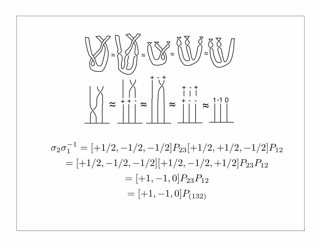
~~
+ +
~~+
~~- -
~~
-
Figure 5: The Twist
~~~~
~~ ~~
~~~~+
+ +
+ +
+
- -
-
-
--
Figure 6: List
~~ ~~ ~~ ~~
~~ + -- -~~
+
~~ +
+-
-
-11 0~~+
++
Figure 7: A Product
7
It will be understood that for the equivalence relation on surfaces consisting ofa disk with three attached bands, a product with framing entirely on the left, andpermutations on the right corresponds to three parallel (unbraided) framed bandsattached to a disk at the bottom of the strands. See Figure 7 for an illustrationof this multiplication process. In that figure we begin with 1
1 2, a braidingof bands with no twisting. If we write out this product using the equivalencerelation derived from the belt deformation we obtain
11 2 = [1/2, 1/2,1/2]P12[1/2,1/2,1/2]P23 =
[1/2, 1/2,1/2][1/2, 1/2,1/2]P12P23 = [0, 1,1]P12P23.
From this, we conclude that 11 2 as a braided disk with bands is equivalent to
an unbraided disk with bands such that the first band has framing 0, the secondband has framing 1 and the third band has framing 1. This is illustrated alsoas a topological deformation in Figure 7.
Here are some specific calculations using this arithmetic.
1 = [1/2,1/2,+1/2]P12
11 = [+1/2,+1/2,1/2]P12
2 = [+1/2,1/2,1/2]P23
12 = [1/2,+1/2,+1/2]P23
211 = [+1/2,1/2,1/2]P23[+1/2,+1/2,1/2]P12
= [+1/2,1/2,1/2][+1/2,1/2,+1/2]P23P12
= [+1,1, 0]P23P12
= [+1,1, 0]P(132)
Here we use (132) to denote the cylic permutation that takes 1 to 3, 3 to 2and 2 to 1.
(211 )3 =
= [+1,1, 0]P(132)[+1,1, 0]P(132)[+1,1, 0]P(132)
= [+1,1, 0]P(132)[+1,1, 0][1, 0,+1]P(132)P(132)
= [+1,1, 0]P(132)[0,1,+1]P(132)P(132)
= [+1,1, 0][1,+1, 0]P(132)P(132)P(132)
= [0, 0, 0]I.
Here I is the identity permutation. Thus
(211 )3 = I.
This means that a belt braided in the pattern (211 )3 can be made from a strip
of leather that has been slit in three parallel strands. This fact is illustrated inFigure 4.
8
~~~~
Figure 4: Braiding a Belt
braid B. They will get permuted in the process, according to the permutation(B) associated with the braid B. Thus
[r, s, t]B[r, s, t]B = [r, s, t][r, s, t](B)BB
where [r, s, t][x, y, z] = [r + x, s + y, t + z] and BB denotes the usual product ofbraid words.
For example,
[r, s, t]1[x, y, z]2 = [r, s, t][y, x, z]12 = [r + y, s + x, t + z]12
.
With the braided leather belts, we have three ribbon strands as shown inFigures 2,3 and 4. The result is three strands bound at top and bottom as shownin these figures. As the figures indicate, the braid representation formalismshows how to rewrite a braided leather belt in the form of twisted parallelstrips.
We see from Figure 2 that [1/2,1/2, 0]11 , (This is Twist1 in the Figure
2) representing three strips with framings as indicated by [1/2,1/2, 0] and
5

~~
~~ ~~
~
e+
boundary( )e+
e+
Figure 8: The Positron
well-defined way. If we simply regard them as braided belts, then it is possible toget dierent products by first deforming the belt of an individual particle, andthen multiplying. This means that the framed braid formulation is probablynecessary for dealing with particle interactions, and it leads to the question ofhow to think physically about ”particles” that have to be in a specific topologicalform in order to combine correctly. This is a challenge for the physics of thesituation. Here is an example: u = [0, 1, 1]2
11 and d = 1
12 [0, 0,1]. Thus
in this form we have ud = [0, 1, 0]. However, if we reduce each of u and d totwisted parallel strands, then we get u [1, 0, 1] and d [1,1, 1]. Evidently[1, 0, 1][1,1, 1] = [0,1, 2] gives a dierent result from the direct compositionof the framed braids.
4 Algebra
In this section we give a representation of the three-strand braid group thatis particularly useful for understanding the properties of braided belts and theparticle theory that we have discussed in the previous section. This representa-tion generalizes to the n-strand braid group, and we shall comment on this atthe end of this section.
10
The Positron and Its Linked Boundary
The recipe for these calculations is to write the braid in terms of the gen-erators ↵1 and ↵2 of the three-strand braid group, and add twisting the stripsby using the framing vectors [a, b, c]. Then rewrite the product, as we did inthe above paragraph so that it has the form [a, b, c]P where P is a product ofpermutation matrices. Then the twisted parallel strip framings are given by thevector [a, b, c].
In this system we represent the braided belt by using a framed braid grouprepresentation and the equivalence relation that is suggested by Figure 1. Notethat in our braid group representation we have ↵1 = [1/2,1/2,+1/2]P12 and,as in Figure 1, this corresponds to the fact the flat braid corresponding to ↵1
deforms to the belt surface with three parallel belts, each with half-twists oftype [1/2,1/2, 1/2]. Thus, we arrive at the follwing result.
Theorem. To determnine the parallel twisted belt form of a framed braidproduct B where B denotes a product of framed braids, apply the braid grouprepresentation and reduce B to the form [a, b, c]P where P is a permuation.Then [a, b, c] is the framing on a topologically equivalent parallel strip form ofthe braided belt. Note that in this representation, we have only rooted thebottom of the belt as shown in Figure 1. We keep the order and position of thetop strands of the belt fixed.
Example 1. The braided belt corresponding to (↵2↵11 )3 is topologically equiv-
alent to three untwisted parallel strips. This means that the belt with this braid-ing can be made from an untwisted belt of parallel strips by an isotopy. Ouralgebraic model shows this since, as we calculated above, (↵2↵
11 )3 == [0, 0, 0]I
where I is the identity permutation.
Example 2. Let e+ = [1, 1, 1]↵11 ↵2. This is Sundance’s positron [2]. We find
that
e+ = [1, 1, 1]↵11 ↵2 = [1, 1, 1][1/2, 1/2,1/2]P12[1/2,1/2,1/2]P23
= [1, 1, 1][1/2, 1/2,1/2][1/2, 1/2,1/2]P12P23 = [1, 2, 0]P12P23.
Thus [1, 2, 0] gives the framings on the equivalent parallel flat strip belt. See Fig-ure 8 for a graphical version of this calculation, and a depiction of the boundaryof the surface that corresponds to e+. We denote the boundary of this surfaceby e+. Note that e+ is independent (topologically) of the deformation thatwe have applied to straighten out the braiding from the original definition ofe+. Thus our algebraic reduction gives us an algorithm for finding the boundarylink for each particle on Bilson’s tables. We return to the whole table at theend of this section.
Example 3. Note that for particle interactions we want well-defined operationson the bits of topology. If we take the particles as shown in Sundance’s paperand regard them in the braid group representation, we can then multiply in a
9
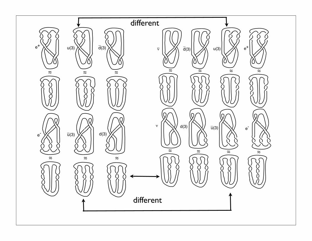
~~
e+
~~ ~~
~~ ~~ ~~
u(3) d(3)
e- u(3)_
_
d(3)
Figure 11: Table 1
12
~~
e+
~~ ~~
~~ ~~ ~~
u(3)d(3)
e-u(3)_
_
d(3)
_
~~ ~~
~~ ~~
Figure 12: Table 2
A permutation matrix P is a matrix whose columns are a permutation ofthe rows of the identity matrix. Such a matrix acts as a permutation on thestandard basis (column vectors that have a single unit entry). We shall refer toP as a permutation. If D is a diagonal matrix and P is a permutation matrix,then
PD = DP P
where DP denotes the result of permuting the elements of D along the diagonalaccording to the permutation P.
Let [a, b, c] denote the matrix
[a, b, c] =
ta 0 00 tb 00 0 tc
.
Let
P12 =
0 1 01 0 00 0 1
and
P23 =
1 0 00 0 10 1 0
.
Note that P12 and P13 are permutation matrices, and that they generate (bytaking products) all permutations on three letters.
13
different
different

Apparent Moral:There is topological
persistence in particle propertiesfor the surfaces.
To what extent do the surfaces represent the elementary particles?
To what extent does the framed braid and/or its algebraic representation
represent theelementary particles?

Algebra Appendix
~~
e+
~~ ~~
~~ ~~ ~~
u(3)d(3)
e-u(3)_
_
d(3)
_
~~ ~~
~~ ~~
Figure 12: Table 2
A permutation matrix P is a matrix whose columns are a permutation ofthe rows of the identity matrix. Such a matrix acts as a permutation on thestandard basis (column vectors that have a single unit entry). We shall refer toP as a permutation. If D is a diagonal matrix and P is a permutation matrix,then
PD = DP P
where DP denotes the result of permuting the elements of D along the diagonalaccording to the permutation P.
Let [a, b, c] denote the matrix
[a, b, c] =
ta 0 00 tb 00 0 tc
.
Let
P12 =
0 1 01 0 00 0 1
and
P23 =
1 0 00 0 10 1 0
.
Note that P12 and P13 are permutation matrices, and that they generate (bytaking products) all permutations on three letters.
13
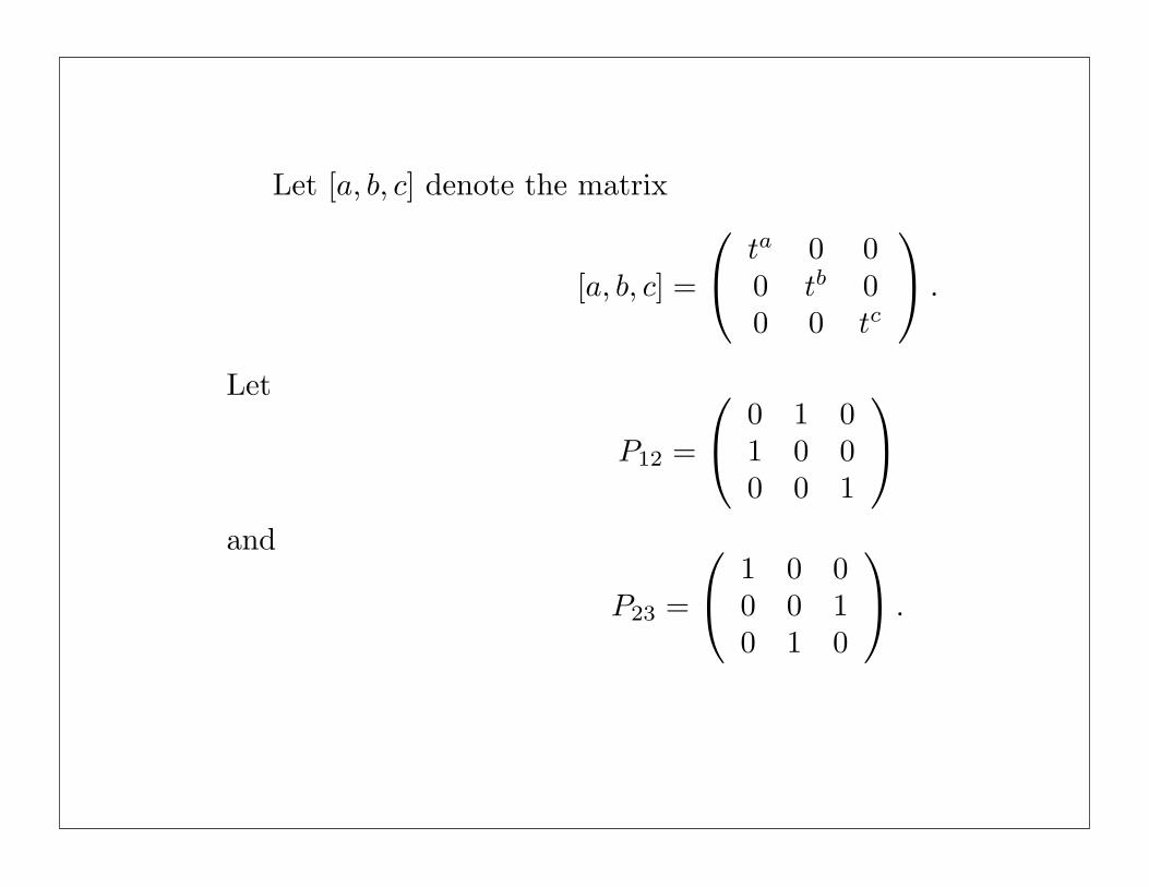

We now define a representation of the three-strand braid group B3 by theequations below. For simplicity we write i for the matrix that represents thisbraid. The reader should understand that the braid is distinct from this matrix,and that in the case of this representation, the matrices do not give a completeimage of the braid group.
1 =
0 t1/2 0
t1/2 0 00 0 t1/2
and
2 =
t1/2 0 00 0 t1/2
0 t1/2 0
.
We leave it to the reader to check that this assignment of matrices gives arepresentation of B3. The only thing to check is the equation 121 = 212.In fact, note that
[a, b, c][d, e, f ] = [a + d, b + e, c + f ]
and, using the formula PD = DP P, we have
P12[a, b, c] = [b, a, c]P12
andP23[a, b, c] = [a, c, b]P23.
Thus we can write1 = [1/2,1/2, 1/2]P12
and2 = [1/2,1/2,1/2]P23
and calculate as follows:
121 = [1/2,1/2, 1/2]P12[1/2,1/2,1/2]P23[1/2,1/2, 1/2]P12
= [1/2,1/2, 1/2][1/2, 1/2,1/2]P12P23[1/2,1/2, 1/2]P12
= [1, 0, 0]P12P23[1/2,1/2, 1/2]P12
= [1, 0, 0]P12[1/2, 1/2,1/2]P23P12
= [1, 0, 0][1/2,1/2,1/2]P12P23P12
= [1/2,1/2,1/2]P12P2,3P12.
Similarly, we find that
212 = [1/2,1/2,1/2]P2,3P12P23.
Since, P12P23P12 = P23P1,2P23, we conclude that 121 = 212.
14
This is the (framed) braid grouprepresentation with which we have
been working.