knots and links from random projection - arxiv · knots and links from random projections by...

Knots and Links from Random ProjectionsBy

Christopher David [email protected]

AbstractIn this paper we study a model of random knots obtained by fixing a space curve in

n-dimensional Euclidean space with n > 3, and orthogonally projecting the space curve onto random 3 dimensional subspaces. By varying the space curve we obtain different modelsof random parametrized knots, and we will study how the expectation value of the curvaturechanges as a function of the initial parametrized space curve. In the case when the initial datais a pair of space curves, or more generally a pair of manifolds satisfying certain conditionson their dimension, then we obtain models of random links for which we will give methods tocompute the second moment of the linking number. As an application of our computations,we will study numerous models of random knots and links, and how to recover these modelsby appropriately choosing the initial space curves to be projected.

i

arX

iv:1

602.

0148

4v3

[m

ath.

PR]

17

Jun

2019

mailto:[email protected]

Contents

1 Introduction 21.1 Informal Overview and Historical Motivation . . . . . . . . . . . . . . . . . . 2

1.1.1 The Model . . . . . . . . . . . . . . . . . . . . . . . . . . . . . . . . . 21.1.2 Configuration Space Integrals and Invariants . . . . . . . . . . . . . . 3

1.2 Summary of the Main Results . . . . . . . . . . . . . . . . . . . . . . . . . . 6

2 Expectation Values 82.1 Background . . . . . . . . . . . . . . . . . . . . . . . . . . . . . . . . . . . . 82.2 Integration Over 3-Dimensional Subspaces . . . . . . . . . . . . . . . . . . . 8

2.2.1 Average Intercrossing Number: 〈ICN〉 . . . . . . . . . . . . . . . . . . 82.2.2 Total Curvature . . . . . . . . . . . . . . . . . . . . . . . . . . . . . . 11

2.3 Integration Over Configuration Spaces . . . . . . . . . . . . . . . . . . . . . 13

3 Second Moment of the Linking Number 173.1 Integration Over 2-Dimensional Subspaces and the Winding Number . . . . 173.2 Integration Over 3-Dimensional Subspaces . . . . . . . . . . . . . . . . . . . 203.3 Integration Over the Stiefel Manifold . . . . . . . . . . . . . . . . . . . . . . 263.4 Integration Over the Configuration Space . . . . . . . . . . . . . . . . . . . . 29

4 Second Moments for Higher Dimensional Linking Integrals 334.1 Integration Over Codimension-1 Subspaces . . . . . . . . . . . . . . . . . . . 33

5 Numerical Study: Petal Diagrams 385.1 Model Details . . . . . . . . . . . . . . . . . . . . . . . . . . . . . . . . . . . 385.2 Expected Total Curvature . . . . . . . . . . . . . . . . . . . . . . . . . . . . 395.3 〈Lk2〉 . . . . . . . . . . . . . . . . . . . . . . . . . . . . . . . . . . . . . . . . 40

6 Future Directions 426.1 Finite Type Invariants . . . . . . . . . . . . . . . . . . . . . . . . . . . . . . 42

A Petal Diagrams (Python Implementation) 48A.1 Python . . . . . . . . . . . . . . . . . . . . . . . . . . . . . . . . . . . . . . . 48A.2 Wolfram Mathematica . . . . . . . . . . . . . . . . . . . . . . . . . . . . . . 51

B Wolfram Mathematica Numerical Implementation of the Degree 2 Vas-siliev Invariant 55

1

Chapter 1

Introduction

1.1 Informal Overview and Historical Motivation

Over the past few decades numerous models of random knots and links have been studied andwere developed either with a specific application in mind, or with the hope that the modelwill be sufficiently universal in the sense that it avoids biasing certain knots and links. Modelsinclude closed random walks on a lattice, random knots with confinement, random equilateralpolygons, random kinematical links, random knots from billiard diagrams, random Fourierknots (for the aforementioned see [2],[4], [12],[15], for example), diagrams sampled fromrandom 4-valent graphs (by Dunfield et. al...see SnapPy documentation: [13]), and therecent Petaluma model studied in [16], [17]. The distributions of the invariants depend onthe details of the models, and the difficulty in computing certain statistics resides in thesampling method. Given this vast list, the question of whether or not there is a universalmodel of random knotting and linking that may contain some of the aforementioned modelsas special cases remains both ill-posed and unexplored. In this paper we seek to explore thisquestion by introducing a further model of random knots which is sufficiently general thatit may be able to encompass some previously studied models of random knots and links.

1.1.1 The Model

In this paper we will consider a model of random knots and links given by first fixing a closedspace curve (or pair of closed space curves in the case of links) r(t) : S1 → Rn with n > 3, andthen choosing a 3 dimensional subspace in Rn at random to project the curve r(t) on to. Theimage under the projection of r(t) is a parametrized knot in R3 for which one may computea number of quantities associated to the space curve, like the curvature and the writhe. Ourhope is to compute the mean and variance of quantities like the curvature, writhe, and linkingnumber with respect to the unique normalized O(n) invariant measure on the Grassmannianof 3-dimensional subspaces in Rn. The rotational invariance of the measure along with thenumerous scaling and multilinearity properties of the aforementioned quantities will allowus to greatly simplify the calculations involved. By choosing different initial curves r(t) inRn, we will obtain different models of knots and links, and moreover we will expect that thedistribution of invariants associated with such models to have a crucial dependence on r(t).

2

1.1. Informal Overview and Historical Motivation

1.1.2 Configuration Space Integrals and Invariants

Since the random knots and links that will be generated with the model described in theprevious section will be parametrized, then the sort of quantities that we will consider willbe ones that have descriptions as configuration space integrals. In the case of links, onesuch invariant is the linking number, and when the components of the link are given bynon-intersecting differentiable curves, γ1 and γ2, given by the parametrizations γ1 = r1(t)and γ2 = r2(s), then the linking number may be computed using the Gauss linking integral:

Lk(γ1, γ2) =1

4π

∫(s,t)∈T2

(r1(t)× r2(s)) · (r2(s)− r1(t))

‖r2(s)− r1(t)‖3dA (1.1.1)

where T2 = S1 × S1 is the torus where each factor is the interval[0, 2π

]with its endpoints

identified, and dA = dsdt. As motivation, we will use the model described in the previoussection to find the expected value of a closely related quantity, the average inter-crossingnumber, which we will denote ICN (see [14] for futher details):

ICN(γ1, γ2) =1

4π

∫(s,t)∈T2

|(r1(t)× r2(s)) · (r2(s)− r1(t))|‖r2(s)− r1(t)‖3

dA

To do so, let γ1 = r1(t) and γ2 = r2(s) be differentiable closed space curves in R4 and definev = (v1, v2, v3, v4) and dv = exp(−1

2(v2

1 +v22 +v2

3 +v24))dv1dv2dv3dv4. This way, we have that:

〈ICN〉 =1

4π(2π)2

∫v∈R4

∫T2

|Det[r1(t), r2(s), r2(s)− r1(t), v

‖v‖

]|

‖projv⊥(r2(s)− r1(t))‖3dsdtdv

where projv⊥(r2(s)− r1(t)) denotes the orthogonal projection on to the orthogonal comple-ment of v

‖v‖ . In order to emphasize the dependence on the initial data r1(t) and r2(s), wewill reverse the order of integration:

〈ICN〉 =1

4π(2π)2

∫T2

∫v∈R4

|Det[r1(t), r2(s), r2(s)− r1(t), v

‖v‖

]|

‖projv⊥(r2(s)− r1(t))‖3dvdA

Next, given vectors a1, a2, a3 ∈ Rn define a matrix A by making the vectors ai the columns,which from now on we will denote by A =

[a1, a2, a3

], and then define the function:

I〈ICN〉(A) =1

(2π)2

∫v∈R4

|Det[a1, a2, a3,

v‖v‖

]|

‖projv⊥(a3)‖3dv (1.1.2)

3


where[a1, a2, a3,

v‖v‖

]∈ Mat4,4. Given the definition in (1.1.2), we may simplify the formula

for 〈ICN〉 as:

〈ICN〉 =1

4π

∫T2

I〈ICN〉([r1(t), r2(s), r2(s)− r1(t)

])dsdt

It will be shown in the following sections that I〈ICN〉([a1, a2, a3

]) has an especially nice form,

and is given by:

I〈ICN〉([a1, a2, a3

]) =√

Det([

a1, a2, a3

]T [a1, a2, a3

])‖a3‖3

, (1.1.3)

so that:

〈ICN〉 =1

4π

∫T2

I〈ICN〉([r1(t), r2(s), r2(s)− r1(t)

])

=1

4π

∫T2

√Det(

[r1(t), r2(s), r2(s)− r1(t)

]T [r1(t), r2(s), r2(s)− r1(t)

])

‖r2(s)− r1(t)‖3dsdt (1.1.4)

For the most part, the goal of this work will be to both find closed forms and understand theanalytic properties of functions like I〈ICN〉(

[r1(t), r2(s), r2(s) − r1(t)

]). By performing this

procedure of reversing the order of integration, and then integrating over all projections, wemay then find bounds on 〈ICN〉 in terms of the parametrization of the initial space curvesr1(t) and r2(s). The computation leading to (1.1.4) will be completed in the second chapter,along with a similar analysis for 〈κ(C)〉, where κ(C) is the total curvature of a knot (thetotal curvature case is not a new result, and was already discovered in a classic paper by[18], [25], and can be found in recent papers such as [29]).

Since κ(C) and 〈ICN〉 are not invariants, but are only bounds on invariants of knots andlinks, then it will be a bit more interesting to consider instead 〈Lk2〉 and the correspondingfunction I〈Lk2〉(A,A

′) obtained from reversing the order of integration as was demonstratedabove. Given two space curves γ1 and γ2 with parametrizations r1(t) and r2(s), then we maycompute the value of Lk2(γ1, γ2) from the Gauss linking integral by computing:

Lk2(γ1, γ2) =

1

16π2

∫(s,t)∈T2

∫(s′,t′)∈T2

Det[r1(t), r2(s), r2(s)− r1(t)

]Det[r1(t′), r2(s′), r2(s′)− r1(t′)

]‖r2(s)− r1(t)‖3‖r2(s′)− r1(t′)‖3

dsdtds′dt′

Figure 1.1.2 depicts the configurations of pairs of points that we will typically want tointegrate over in order to find the value of Lk2(γ1, γ2).

4


Figure 1.1.1: The geometric configuration for computing Lk2 for the closed space curvesr1(s) and r2(t) where a3(s, t) = r2(s)− r1(t) and a3(s′, t′) = r2(s′)− r1(t′)

Obtaining I〈Lk2〉(A,A′) in this case is considerably more difficult, and will occupy the third

chapter, which is the main part of this work. The computation involved after switching theorder of integration is summarized with the following lemma:

Lemma 1.1.1. Given matrices A =[a1,a2,a3

], A′ =

[a′1,a

′2,a

′3

]∈ Mat4,3 and the function

I〈Lk2〉(A,A′) =

1

(2π)2

∫R4

Det([A v‖v‖ ])Det([A′ v

‖v‖ ])

‖projv⊥(a3)‖3‖projv⊥(a′3)‖3e−‖v‖

2/2dv

where[A v‖v‖

]denotes a new matrix in Mat4,4 with the column v

‖v‖ appended to the matrixA, then we have

π

2I〈Lk2〉(A,A

′) =

(‖a3‖2‖a′3‖2 − (a3 · a′3)2)Det(ATA′) + (a3 · a′3)Det([a3,a

′1,a

′2,a

′3

])Det(

[a′3,a1,a2,a3

])

‖a3‖2‖a′3‖2(‖a3‖2‖a′3‖2 − (a3 · a′3)2)3/2

It will be seen throughout the course of the proof of the above lemma that the requirementthat the initial spaces curves r1(t) and r2(s) be embedded in R4 serves to simplify theintegration over Gr(4, 3) since the subspaces we are integrating over are codimension 1 sothat Gr(4, 3) ∼= S3. This restrictive assumption will be removed in the second half of chapter3 by introducing the Stiefel manifold of orthonormal 3-frames in Rn, denoted Vn,3, and usinga decomposition of its unique normalized O(n) measure coupled with the previous result inorder to find 〈Lk2〉 for any pair of curves in Rn, for n sufficiently large.

5

1.2. Summary of the Main Results

1.2 Summary of the Main Results

Theorem 1.2.1. Given two closed, differentiable, non-intersecting space curves γ1, γ2 : S1 →Rn with parametrizations r1(t) and r2(s), and let projU(γ1), projU(γ2) denote the orthogonalprojections of γ1 and γ2 on to the 3 dimensional subspace spanned by the columns of U , thenthe expected value of ICN(projU(γ1), projU(γ1)), denoted 〈ICN〉, averaged over all orthogonalprojections to 3 dimensional subspaces with respect to the unique normalized O(n)-invariantmeasure on Gr(n, 3), is given by the following integral:

〈ICN〉 =1

4π

∫(s,t)∈T2

I〈ICN〉(s, t)dsdt

where

I〈ICN〉(s, t) = C〈ICN〉

√Det(

[dr1(t)dt

, dr2(s)ds

, r2(s)− r1(t)]T [dr1(t)

dt, dr2(s)

ds, r2(s)− r1(t)

])

‖r2(s)− r1(t)‖3,

where C〈ICN〉 is a constant.

After proving the above theorem we then focus on the computation of 〈ICN〉:

Theorem 1.2.2. Let r1(t) : S1 → R2n+1 and r2(s) : S1 → R2n+1 be given by:

r1(t) = c0e0 +n∑k=1

(ck cos(kt)e2k−1 + ck sin(kt)e2k)

= (c0, c1 cos(t), c1 sin(t), c2 cos(2t), c2 sin(2t), ..., , cn cos(nt), cn sin(nt)), and

r2(s) = d0e0 +n∑k=1

(ck cos(ks)e2k−1 + ck sin(ks)e2k)

= (d0, d1 cos(s), d1 sin(s), d2 cos(2s), d2 sin(2s), ..., , dn cos(ns), dn sin(ns)),

where eini=1 are the standard basis vectors, then 〈ICN〉 is finite and satisfies the followingbound:

〈ICN〉 ≤ C〈ICN〉

√(∑n

j=0 j2c2j)(∑n

j=0 j2d2j)

min(s,t)∈T2‖r2(s)− r1(t)‖2

In chapter 3 we move on to proving the main theorem of the paper concerning the secondmoment of the linking number.

Theorem 1.2.3. Given two closed, differentiable, non-intersecting space curves γ1, γ2 : S1 →Rn with parametrizations r1(t) and r2(s), and let projU(γ1), projU(γ2) denote the orthogonalprojections of γ1 and γ2 on to the 3 dimensional subspace spanned by the columns of U , thenthe expected value of Lk2(projU(γ1), projU(γ2)), denoted 〈Lk2〉, averaged over all orthogonalprojections to 3 dimensional subspaces with respect to the unique normalized O(n)-invariant

6

1.2. Summary of the Main Results

measure on Gr(n, 3), is given by the following integral:

〈Lk2〉 =1

16π2

∫(s,t)∈T2

∫(s′,t′)∈T2

I〈Lk2〉(A(s, t), A′(s′, t′))dsdtds′dt′

where

π

4I〈Lk2〉(A,A

′) =

(a3 · a′3)−√‖a3‖2‖a′3‖2 − (a3 · a′3)2 sin−1

(a3·a′3‖a3‖‖a′3‖

)(a3 · a′3)3

√‖a3‖2‖a′3‖2 − (a3 · a′3)2

Det

a1 · a′1 a1 · a′2 a1 · a′3a2 · a′1 a2 · a′2 a2 · a′3a3 · a′1 a3 · a′2 a3 · a′3

and

a1 = r1(t),a2 = r2(s),a3 = r2(s)− r1(t)

a′1 = r1(t′),a′2 = r2(s′),a′3 = r2(s′)− r1(t′)

A =[r1(t), r2(s), r2(s)− r1(t)

]A′ =

[r1(t′), r2(s′), r2(s′)− r1(t′)

]After integrating over all the projections, we then turn our attention to integrating over

the configuration space.

Theorem 1.2.4. With the definitions above, let v1 = maxt∈S1‖r1(t)‖, v2 = maxs∈S1‖r2(s)‖,k = min(s,t)∈T2‖r2(t)− r1(s)‖ and

C =

∫ 2π

0

∫ 2π

0

∫ 2π

0

∫ 2π

0

1√‖a3(s, t)‖2‖a′3(s′, t′)‖2 − (a3(s, t) · a′3(s′, t′))2

dsdtds′dt′,

then

〈Lk2〉 ≤ 1

(4π)2

4Cv21v

22

πk2

That is, we obtain a bound on the second moment of the linking number provided theinitial space curves are chosen so that v1, v2 and C are finite. In the fourth chapter we willprove theorems very analogous to theorems in chapter 3 concerning the second moment oflinking numbers associated to manifolds as defined in [28]. Lastly, in order to show theapplicability of some of our results, in the penultimate chapter we consider a model that isvery similar to the model in [16].

7

Chapter 2

Expectation Values

2.1 Background

In the first part of this chapter we will find the expectation value of 〈ICN〉 when we fix apair of space curves in R4 and project the curves randomly on to 3 dimensional subspaces.As discussed in the introduction, this will require two steps, the first will be integrating overall 3 dimensional subspaces, and then integrating that result over the configuration spaceof two points on distinct components of a link. The first step can be done exactly, whereasthe second will be approached by making specific assumptions about the initial data. In thesecond part of this chapter we will find the expected curvature when we fix one space curvein Rn, and project the curve randomly on to 3 dimensional subspaces, where we pick randomsubspaces by sampling the spans of the columns of Gaussian random matrices in Matn,3.

2.2 Integration Over 3-Dimensional Subspaces

2.2.1 Average Intercrossing Number: 〈ICN〉We start with the following lemma:

Lemma 2.2.1. Given a matrix A =[a1,a2,a3

]∈ Mat4,3 and the function

I〈ICN〉(A) =1

(2π)2

∫R4

|Det([A v‖v‖ ])|

‖projv⊥(a3)‖3e−‖v‖

2/2dv

where[A v‖v‖

]denotes a new matrix in Mat4,4 with the column v

‖v‖ appended to the matrixA, then we have

I〈ICN〉([a1,a2,a3

]) =

√Det

([a1,a2,a3

]T [a1,a2,a3

])‖a3‖3

,

8

2.2. Integration Over 3-Dimensional Subspaces

Proof We first observe the following properties of I〈ICN〉([a1, a2, a3

]):

I〈ICN〉

A k1 0 0

0 k2 00 0 k3

=| k1 || k2 || k3 |2

I〈ICN〉(A) (2.2.1)

I〈ICN〉

A

1 0 0−a1·(a2− a2·a3

‖a3‖2a3)

‖(a2− a2·a3‖a3‖2

a3‖1 0

−a1·a3

‖a3‖2−a2·a3

‖a3‖2 1

= I〈ICN〉(A) (2.2.2)

Using (2.2.2) we may make the columns orthogonal, and then using (2.2.1) we may furthermake them orthonormal. Next, using the fact that the measure e−‖v‖

2/2dv is O(4) invariant,we may take the orthonormal set of vectors to coincide with the standard basis vectors,e1, e2, e3 so that I〈ICN〉(A) may be rewritten as:

I〈ICN〉(A) =f(a1, a2, a3)

(2π)2

∫v∈R4

| Det([e1 e2 e3v‖v‖ ]) |

‖projv⊥(a3)‖3exp(−‖v‖

2

2)dv

= f(a1, a2, a3)I|Lk|([e1, e2, e3

]),

where

f([a1 a2 a3]) =

‖a1 −a1·(a2− a2·a3

‖a3‖2a3)

‖(a2− a2·a3‖a3‖2

a3‖(a2 − a2·a3

‖a3‖2 a3)− a1·a3

‖a3‖2 a3‖‖a2 − a2·a3

‖a3‖2 a3‖‖a3‖

‖a3‖3

=

√Det(ATA)

‖a3‖3, and

Now we will compute the integral:

I〈ICN〉(A) =1

(2π)2f([a1 a2 a3])

∫R4

| Det([e1 e2 e3v‖v‖ ]) |

‖projv⊥(e3)‖3exp(−‖v‖

2

2)dv

=1

(2π)2f([a1 a2 a3])

∫R4

| v4/‖v‖ |‖projv⊥(e3)‖3

exp(−‖v‖2

2)dv

=1

(2π)2f([a1 a2 a3])

∫R4

| v4/‖v‖ |(‖v‖2−v23‖v‖2 )3/2

exp(−‖v‖2

2)dv =

=1

(2π)2f([a1 a2 a3])

∫R4

‖v‖2 | v4 |(‖v‖2 − v2

3)3/2exp(−‖v‖

2

2)dv = f([a1 a2 a3])

9


Given two space curves r1(t) and r2(s) in R4, if we set

a1(t) =dr1(t)

dt

a2(s) =dr2(s)

dsa3(t, s) = r2(s)− r1(t) and

A(s, t) =[a1(t), a2(s), a3(s, t)

]in the previous lemma, then we will have the following lemma:

Lemma 2.2.2. Given two differentiable, non-intersecting space curves r1(t) and r2(s) in R4,then the value of ICN averaged over all orthogonal projections to 3 dimensional subspaceswith respect to the unique normalized O(4)-invariant measure on Gr(4, 3), is given by thefollowing integral:

〈ICN〉 =1

4π

∫(s,t)∈T2

I〈ICN〉(A(s, t))dsdt

Proof Consider the integral, I〈ICN〉(A), from the previous lemma. We may integrate overv = v1, v2, v3, v4 by changing to 4-dimensional spherical coordinates where

v1 = r cos(φ1)

v2 = r sin(φ1) cos(φ2)

v3 = r sin(φ1) sin(φ2) cos(φ3)

v4 = r sin(φ1) sin(φ2) sin(φ3)

so that e−‖v‖2/2dv = e−r

2/2r3 sin2(φ1) sin(φ2)drdφ1dφ2dφ3 and r ∈[0,∞), φ1 ∈

[0, π], φ2 ∈[

0, π], φ3 ∈

[0, 2π). Since the function we are integrating against e−r

2/2r3 sin2(φ1) sin(φ2)drdφ1dφ2dφ3

is invariant under scaling v, then we may integrate out the radial coordinate r in order toobtain an integral over a 3-sphere, and the result follows from the previous lemma sinceS3 ∼= Gr(4, 3) and since Gr(4, 3) has a unique normalized O(4) invariant measure on it.

Using the techniques in [33] and that we will develop in the proof of 1.2.3, it is straight-forward to show that:

Theorem 1.2.1.Given two closed, differentiable, non-intersecting space curves γ1, γ2 : S1 →Rn with parametrizations r1(t) and r2(s), and let projU(γ1), projU(γ2) denote the orthogonalprojections of γ1 and γ2 on to the 3 dimensional subspace spanned by the columns of U , thenthe expected value of ICN(projU(γ1), projU(γ2)), denoted 〈ICN〉, averaged over all orthogonalprojections to 3 dimensional subspaces with respect to the unique normalized O(n)-invariantmeasure on Gr(n, 3), is given by the following integral:

〈ICN〉 =1

4π

∫(s,t)∈T2

I〈ICN〉(s, t)dsdt

10


where

I〈ICN〉(s, t) = C〈ICN〉

√Det(

[dr1(t)dt

, dr2(s)ds

, r2(s)− r1(t)]T [dr1(t)

dt, dr2(s)

ds, r2(s)− r1(t)

])

‖r2(s)− r1(t)‖3,

where C〈ICN〉 is a constant.

Proof We will focus only on integrating over Matn,3, since the integration over Gr(n, 3)follows easily from the following computation and the discussion in the next chapter. Definethat:

I〈ICN〉([a1, a2, a3

]) =

1

(2π)3n/2

∫U∈Matn,3

√Det(

[a1, a2, a3

]TU(UTU)−1UT

[a1, a2, a3

])

(aT3U(UTU)−1UTa3)3/2dU,

where we think of U ∈ Matn,3 as a matrix with columns u1,u2 and u3, and

dU = exp(−1

2Tr(UTU))du1du2, du3

Next, apply the Gram-Schmidt process to the ordered set of vectors a3, a2, a1 to obtainthe orthonormal set q3,q2,q1, so that we have:

I〈ICN〉([a1, a2, a3

]) =

1

(2π)3n/2

Det(ATA)1/2

‖a3‖3

∫U∈Matn,3

√Det(

[q1,q2,q3

]TU(UTU)−1UT

[q1,q2,q3

])

(qT3U(UTU)−1UTq3)3/2dU

=Det(ATA)1/2

‖a3‖3I〈ICN〉(

[q1,q2,q3

]),

where in the above A =[a1, a2, a3

]. Since the measure dU is O(n) invariant, then we

may take the set of vectors q1,q2,q3 to coincide with the first 3 standard basis vectors:e1, e2, e3. The result follows by setting C〈ICN〉 = I〈ICN〉(e1, e2, e3)

Remark 2.2.3. Notice that if we considered 〈Lk〉 instead, the integral would have vanished.

2.2.2 Total Curvature

For pedagogical purposes, we will apply a similar analysis to find the expected total curvatureof a knot. For the most part, the following is due to Fary [18], Milnor [25], and appears ina more generalized context by Sullivan [29]. In this section, we will simply show that theaforementioned arguments easily fit in to our framework discussed previously. To do so, recallthat if we are given a twice continuously differentiable space curve, C, with parametrizationr(t) : S1 → R3, we may compute the total curvature, κ(C), using a Gauss-like integral:

κ(C) =

∫ 2π

0

|r′(t)× r′′(t)|‖r′(t)‖2

dt =

∫ 2π

0

√‖r′(t)‖2‖r′′(t)‖2 − (r′(t) · r′′(t))2

‖r′(t)‖2dt,

11


First we will prove a lemma analogous to 2.2.1:

Lemma 2.2.4. Given a matrix A =[a1,a2

]∈ Matn,2 and the function

Iκ(C)(A) =1

(2π)3n/2

∫Rn

∫Rn

∫Rn

| Det(ATU(UTU)−1UTA) |1/2

(aT1U(UTU)−1UTa1)2dU

where U denotes the matrix U =[u1,u2,u3

]and dU = exp(−1

2(‖u1‖2+‖u2‖2+‖u3‖2)du1du2du3,

then

Iκ(C)(A) = k

√‖a1‖2‖a2‖2 − (a1 · a2)2

‖a1‖2

where k is a constant.

Proof As in the proof of lemma 2.2.1, we may use the numerous multilinearity and scalingproperties to write Iκ(C)(A) as:

Iκ(C)(A) =1

(2π)3n/2

√|Det(ATA)|‖a1‖2

∫Rn

∫Rn

∫Rn

| Det(U(UTU)−1UT ) |1/2

(U(1)(UTU)−1U(1)

T)2

dU

where U is an n by 3 matrix with columns u1,u2 and u3, and

U =

(u11 u21 u31

u12 u22 u32

)and

U(1) =(u11 u21 u31

),

where uij is the jth entry of the vector ui.

The result follows by setting k = 1(2π)3n/2

∫Rn∫Rn∫Rn|Det(U(UTU)−1UT )|1/2

(U(1)(UTU)−1U(1)

T)2dU.

The following is essentially due to Fary and Milnor:

Theorem 2.2.5. Let C be a twice-differentiable space curve with parametrization r(t) : S1 →Rn and projU(r(t)) be the orthogonal projection of r(t) to the 3-dimensional subspace spannedby the columns of U , then the value of the total curvature, κ(projUr(t))), averaged over allprojections to 3 dimensional subspaces with respect to the Gaussian measure on Matn,3 isgiven by the integral:

〈κ(C)〉 =

∫t∈T1

Iκ(C)(t)dt

where

Iκ(C)(t) =

√‖r′(t)‖2‖r′′(t)‖2 − (r′(t) · r′′(t))2

‖r′(t)‖2

12

2.3. Integration Over Configuration Spaces

Proof Given the twice differentiable curve r(t) : S1 → Rn, we set

a1(t) =dr1(t)

dt

a2(t) =d2r1(t)

dt2

A(t) =[a1(t), a2(t)

]This way we will have that:

〈κ(C)〉 =

∫ 2π

0

Iκ(C)(A(t))dt

Using the previous lemma we have that:

〈κ(C)〉 =

∫ 2π

0

k

√‖a1(t)‖2‖a2(t)‖2 − (a1(t) · a2(t))2

‖a1(t)‖2dt

Since the above holds for any r(t), then in particular we may take r(t) = cos(t)e1 + sin(t)e2,so that 〈κ(C)〉 = 2π since the image of almost all projections will be a planar ellipse. It is

also easy to compute that∫ 2π

0k

√‖a1(t)‖2‖a2(t)‖2−(a1(t)·a2(t))2

‖a1(t)‖2 dt = 2π, so that we see:

1

(2π)3n/2

∫Rn

∫Rn

∫Rn

| Det(U(UTU)−1UT ) |1/2

(UT(1)(U

TU)−1UTUT(1))

2exp−

12

(‖u1‖2+‖u2‖2+‖u3‖2)du1du2du3 = 1

and therefore

〈κ(C)〉 =

∫ 2π

0

√‖r′(t)‖2‖r′′(t)‖2 − (r′(t) · r′′(t))2

‖r′(t)‖2dt (2.2.3)

That is, the expected total curvature of one of the knot projections is simply the totalcurvature of the space curve C that we are randomly projecting to lower dimensions.

2.3 Integration Over the Configuration Space

Up to this point we have only considered the integration over all the 3 dimensional subspaces,and now we will consider how to specify the initial data, so as to bound 〈κ(C)〉 and 〈ICN〉and therefore bound the complexity of the curvature and the average inter-crossing number.We will now prove the following theorem:

13


Theorem 1.2.2. Let r1(t) : S1 → R2n+1 and r2(s) : S1 → R2n+1 be given by:

r1(t) = c0e0 +n∑k=1

(ck cos(kt)e2k−1 + ck sin(kt)e2k)

= (c0, c1 cos(t), c1 sin(t), c2 cos(2t), c2 sin(2t), ..., , cn cos(nt), cn sin(nt)), and

r2(s) = d0e0 +n∑k=1

(ck cos(ks)e2k−1 + ck sin(ks)e2k)

= (d0, d1 cos(s), d1 sin(s), d2 cos(2s), d2 sin(2s), ..., , dn cos(ns), dn sin(ns))

then 〈ICN〉 is finite and satisfies the following bound:


√(∑n

j=0 j2c2j)(∑n

j=0 j2d2j)

min(s,t)∈T2‖r2(s)− r1(t)‖2

Proof By (1.2.1) we have:


∫ 2π

0

∫ 2π

0

‖dr1(t)dt‖‖dr2(s)

ds‖

4πmin(s,t)∈T2‖r2(s)− r1(t)‖2dtds

≤ C〈ICN〉

∫ 2π

0

∫ 2π

0

√(∑n

j=0 j2c2j)(∑n

j=0 j2d2j)

4πmin(s,t)∈T2‖r2(s)− r1(t)‖2dtds

= C〈ICN〉π

√(∑n

j=0 j2c2j)(∑n

j=0 j2d2j)

min(s,t)∈T2‖r2(s)− r1(t)‖2dtds,

so that we may bound 〈ICN〉:

〈ICN〉 ≤ C〈ICN〉π

√(∑n

j=0 j2c2j)(∑n

j=0 j2d2j)

min(s,t)∈T2‖r2(s)− r1(t)‖2

If we make even stronger assumptions, for example that the initial spaces curves beorthogonal, then we can significantly improve the above bound. For example, if the initialspace curves r1(t), r2(s) : S1 → R4N+2 are orthogonal:

r1(t) = c0e1 +N∑k=1

(ck cos(kt)e4k−1 + ck sin(kt)e4k) (2.3.1)

r2(s) = d0e2 +N∑k=1

(dk cos(kt)e4k+1 + dk sin(kt)e4k+2), (2.3.2)

14


then by Hadamard’s inequality we have that:

〈ICN〉 ≤ 1

4π

2π∫s=0

2π∫t=0

CICN‖r′1(t)‖r′2(s)‖‖r2(s)− r1(t)‖2

dsdt = πCICN

√(∑N

k=1 k2c2k)(∑N

k=1 k2d2k)∑N

k=0 c2k +

∑Nk=0 d

2k

Similarly, for the total curvature we have the following theorem:

Theorem 2.3.1. Let r(t) : S1 → R2n+1 be given by:

r(t) = c0e0 +n∑k=1

(ck cos(kt)e2k−1 + ck sin(kt)e2k) (2.3.3)

= (c0, c1 cos(t), c1 sin(t), c2 cos(2t), c2 sin(2t), ..., , cn cos(nt), cn sin(nt)),

then 〈κ(C)〉 is finite and satisfies the following bound:

〈κ(C)〉 ≤ 2π

√∑nk=0 c

2kk

2∑nk=0 c

2kk

4

Proof For 〈κ(C)〉, notice first that:

〈κ(C)〉 ≤∫ 2π

0

‖r′′(t)‖‖r′(t)‖

dt (2.3.4)

‖r′(t)‖2 =n∑k=1

c2kk

2

‖r′′(t)‖2 =n∑k=1

c2kk

4

The quotient ‖r′′(t)‖‖r′(t)‖ has no dependence on t, and so the result follows from (2.3.4) by inte-

grating over t.

Remark 2.3.2. As mentioned in the introduction, since we are considering arbitrary spacecurves in Rn, and since the formulas involved did not have any explicit dependence on n,then we may allow n to approach infinity and consider a space curve of the form:

r(t) = c0e0 +∞∑n=1

(cn cos(nt)e2n−1 + cn sin(nt)e2n) (2.3.5)

= (c0, c1 cos(t), c1 sin(t), c2 cos(2t), c2 sin(2t), ..., , cn cos(nt), cn sin(nt), ...)

In this way, if we define the sequences c = cn∞n=0, c′ = ncn∞n=0, c′′ = n2cn∞n=0 andstipulate that ‖c′′‖l2 < ∞ (that is, the sequence c decays faster than n(−5−ε)/2), then the

quotient ‖r′′(t)‖‖r′(t)‖ will be finite and will give a bound for 〈κ(C)〉 so that with high probability

15


the projections will have bounded total curvature given by:

〈κ(C)〉 ≤∫ 2π

0

‖r′′(t)‖‖r′(t)‖

dt =

∫ 2π

0

√∑∞n=0 n

4c2n∑∞

n=0 n2c2n

dt

and therefore:

〈κ(C)〉 ≤ 2π‖c′′‖l2‖c′‖l2

A similar result holds for 〈ICN〉. In particular, using the data (2.3.1), we will have that:

〈ICN〉 ≤ πCICN‖c′‖l2‖d′‖l2‖c‖2

l2 + ‖d‖2l2, (2.3.6)

so that the sequence c must decay faster than n(−3−ε)/2.

16

Chapter 3

Second Moment of the LinkingNumber

3.1 Integration Over 2-Dimensional Subspaces and the

Winding Number

Before we go on to compute the second moment of the linking number, we would like to firstconsider a simpler case: that of computing the second moment of the winding number for amodel of random plane curves closely related to the model of random knots discussed in theprevious sections. In particular, we fix a space curve in Rn, and project the space curve ontorandom 2 dimensional subspaces of Rn, chosen from the unique O(n) invariant measure onGr(n, 2).

For a differentiable plane curve, r(t), recall that the winding number W can be computedas a degree of a map, which may be written as an integral of the form:

W =1

2π

∫S1

Det [r(t), r′(t)]

‖r(t)‖2dt (3.1.1)

With this definition, we can compute the second moment 〈W 2〉 of the winding number W ,for a given fixed differentiable map r : S1 → Rn. In particular, we compute:

〈W 2〉 =1

(2π)n

∫U∈Matn,2

1

(2π)2

∫S1×S1

Det(UT [r′(t), r(t)])Det(UT [r′(s), r(s)])

‖UT r(t)‖2‖UT r(s)‖2dsdt

e−Tr(UT U)

2 dU

(3.1.2)where U is a Gaussian random matrix. Next, switch the order of integration in (3.1.2) toobtain:

〈W 2〉 =1

(2π)2

∫S1×S1

1

(2π)n

∫U∈Matn,2

Det(UT [r′(t), r(t)])Det(UT [r′(s), r(s)])

‖UT r(t)‖2‖UT r(s)‖2e−Tr(UT U)

2 dU

dsdt

(3.1.3)

17

3.1. Integration Over 2-Dimensional Subspaces and the Winding Number

Now we focus on the Gaussian integral in parentheses, and define:

I(a1, a′1, a2, a

′2) =

1

(2π)n

∫U∈Matn,2

Det(UT [a1, a2])Det(UT [a′1, a′2])

‖UTa2‖2‖UTa′2‖2e−Tr(UT U)

2 dU (3.1.4)

where a1, a′1, a2, a

′2 ∈ Rn so that (3.1.2) becomes:

〈W 2〉 =

∫S1×S1

I (r′(t), r′(s), r(t), r(s)) dsdt (3.1.5)

To compute (3.1.4), first normalize a2 and a′2 to obtain the unit vectors q2 and q′2, andchoose a basis B = b1,b2, ...,bn where b1 and b2 are in the span of q2 and q′2. In whatfollows, for convenience we take decide to take :

b1 =a2‖a′2‖+ a′2‖a2‖√

2 (‖a2‖2‖a′2‖2 + ‖a2‖‖a′2‖(a2 · a′2))

b2 =a2‖a′2‖ − a′2‖a2‖√

2 (‖a2‖2‖a′2‖2 − ‖a2‖‖a′2‖(a2 · a′2))

and we further define that:

a =a2

‖a2‖· b1 = | cos(x/2)|

b =a′2‖a′2‖

· b2 = | sin(x/2)|, (3.1.6)

where x is the angle between a2 and a′2. In this way we have a and b are given just in termsof dot products between a1, a

′1, a2, a

′2, and moreover a2 + b2 = 1. With these defintions, we

then expand the integrand using the multilinearity of the determinant to obtain:

I(a1, a′1, a2, a

′2) =

1

‖a2‖‖a′2‖

n∑i,j=1

a1ia′1jI(ei, ej, ae1 + be2, ae1 − be2),

where hereinafter we define a1i = a1 · bi and similarly a′1i = a′1 · bi, are the components ofa1 and a′1 in the basis B. There are a few cases to consider when we compute I(ei, ej, ae1 +be2, ae1 − be2). The integral I(ei, ej, ae1 + be2, ae1 − be2) has a simple form:

I(ei, ej,ae1 + be2, ae1 − be2)

=

∫U∈Matn,2

Det(

[u1i au11 + bu12

u2i au21 + bu22

])Det(

[u1j au11 − bu12

u2j au21 − bu22

])

((au11 + bu12)2 + (au21 + bu22)2) ((au11 − bu12)2 + (au21 − bu22)2)e−Tr(UT U)

2 dU

Applying a combination of symmetries of the integrand and a few coordinate changes we

18

3.1. Integration Over 2-Dimensional Subspaces and the Winding Number

obtain that:

‖a2‖‖a′2‖I(a1, a′1, a2, a

′2) = (a11a

′12 − a12a

′11) I(e1, e2, ae1 + be2, ae1 − be2)

+

(a11a

′11 −

a2

b2a12a

′12

)I(e1, e1, ae1 + be2, ae1 − be2)

+

(n∑k=3

a1ka′1k

)I(e3, e3, ae1 + be2, ae1 − be2)

In the above, notice that∑n

k=3 a1ka′1k = a1 ·a′1−a11a

′11−a12a

′12, so we do not need to know

b3, ...,bn explicitly, which is a computational convenience. We can in fact simplify theabove even further by writing I(e1, e2, ae1 +be2, ae1−be2) = a

bI(e1, e1, ae1 +be2, ae1−be2) so

that the computation has now simplified to computing two Gaussian integrals: I(e1, e1, ae1+be2, ae1 − be2) and I(e3, e3, ae1 + be2, ae1 − be2).

Both integrals can be simplified to integrals over R4 (two variables of I(e3, e3, ae1 +be2, ae1 − be2) can be easily integrated out), and the radial portion may be integrated outleaving two integrals over a 3-sphere. From here, we choose a coordinate system on the3-sphere:

u11 = cos(σ) cos(θ)

u12 = cos(σ) sin(θ)

u21 = sin(σ) sin(φ)

u22 = sin(σ) sin(φ)

where σ ∈ (0, π/2), η, φ ∈ (0, 2π). This particular coordinate system is convenient, and waschosen with the form of the integrand’s denominator in mind. After integrating over thesphere we obtain:

I(a1, a′1, a2, a

′2) =

log(4a2b2) ((b2 − a2)(a1 · a′1)‖a2‖‖a′2‖+ (a1 · a′2)(a′1 · a2))

2(b2 − a2)2‖a2‖2‖a′2‖2(3.1.7)

where a and b are from (3.1.6). Now we will write (3.1.8) in terms of r(t) and r(s):

I (r′(t), r′(s), r(t), r(s)) =log(sin(x)2) (− cos(x) (r′(t) · r′(s)) ‖r(t)‖‖r(s)‖+ (r′(t) · r(s))(r′(s) · r(t))

2 cos(x)2‖r(t)‖2‖r(s)‖2

where x(s, t) is the angle between r(t) and r(s). Simplifying even further we obtain:

I (r′(t), r′(s), r(t), r(s)) =log(‖r(t)‖2‖r(s)‖2−(r(t)·r(s))2

‖r(t)‖2‖r(s)‖2 ) ((r′(t) · r(s))(r′(s) · r(t))− (r(t) · r(s))(r′(t) · r′(s))))2 (r(t) · r(s))2

(3.1.8)

19


I (r′(t), r′(s), r(t), r(s)) =log(‖r(t)‖2‖r(s)‖2−(r(t)·r(s))2

‖r(t)‖2‖r(s)‖2 ) ((r′(t) · r(s))(r′(s) · r(t))− (r(t) · r(s))(r′(t) · r′(s))))2 (r(t) · r(s))2

(3.1.9)

=

log(‖r(t)‖2‖r(s)‖2−(r(t)·r(s))2

‖r(t)‖2‖r(s)‖2 )Det

([r′(t) · r(s) r(t) · r(s)r′(t) · r′(s) r′(s) · r(t)

])2 (r(t) · r(s))2

(3.1.10)

In summary, we simplified a high dimensional Gaussian integral into several smaller integralsusing the symmetries of the integrand, in order to obtain a function that depended only onthe pairwise dot products of a set of vectors. With this technique developed, in the nextsection, we generalize this argument in order to find the second moment of the linking numberfor the model of random links discussed in previous sections.

3.2 Integration Over 3-Dimensional Subspaces

As stated in the introduction, in order to find the second moment of the linking number fora link whose components γ1 and γ2 are parametrized by r1(t) and r2(s), we must considerthe expectation value of an integral of the form:

Lk2(r1, r2) =

1

(4π)2

∫(s,t)∈T2

∫(s′,t′)∈T2

Det[r1(t), r2(s), r2(s)− r1(t)

]Det[r1(t′), r2(s′), r2(s′)− r1(t′)

]‖r2(s)− r1(t)‖3‖r2(s′)− r1(t′)‖3

dsdtds′dt′,

So, to begin, given the vectors: a1, a2, a3, a′1, a′2, a′3 ∈ Rn define the matrices:

A = [a1, a2, a3]

A′ = [a′1, a′2, a′3]

and define a function I〈Lk2〉 : Matn,3 ×Matn,3 → R by:

I〈Lk2〉(A,A′) =

1

(2π)3n2

∫U∈Matn,3

Det(UTA)Det(UTA′)

‖UTa3‖3‖UTa′3‖3e−Tr(UTU)/2dU. (3.2.1)

With this definition we have that:

〈Lk2(r1, r2)〉 =1

(4π)2

∫(s,t)∈T2

∫(s′,t′)∈T2

I〈Lk2〉(R(s, t),R(s′, t′))dsdtds′dt′

where R(s, t) =[r1(t), r2(s), r2(s)− r1(t)

]and R(s′, t′) =

[r1(t′), r2(s′), r2(s′)− r1(t′)

].

20


Remark 3.2.1. For conciseness, hereinafter we will suppress the dependence on the initialspace curves r1(t) and r2(s) and will henceforth write 〈Lk2〉 to denote 〈Lk2(r1, r2)〉 when thedependence on r1(t) and r2(s) is clear.

In order to find 〈Lk2〉, it will be helpful to determine an explicit form for the integralI〈Lk2〉(A,A

′) and then we will need to integrate over the configuration space of pairs of tuplesof points on distinct components of the link. We will now focus on performing the integralin the expression (3.2.1) for I〈Lk2〉(A,A

′):

Lemma 3.2.2. Given matrices A =[a1,a2,a3

], A′ =

[a′1,a

′2,a

′3

]∈ Matn,3 and the function

I〈Lk2〉(A,A′) =

1

(2π)3n2

∫U∈Matn,3

Det(UTA)Det(UTA′)

‖UTa3‖3‖UTa′3‖3e−Tr(UTU)/2dU.

then we have

π

4I〈Lk2〉(A,A

′) =

(a3 · a′3)−√‖a3‖2‖a′3‖2 − (a3 · a′3)2 sin−1

(a3·a′3‖a3‖‖a′3‖

)(a3 · a′3)3

√‖a3‖2‖a′3‖2 − (a3 · a′3)2

Det


(3.2.2)

Proof To begin, normalize the vectors a3 and a′3 to form the vectors q3 and q′3 respec-tively, and then express (3.2.1) as:

I〈Lk2〉(A,A′) =

1

(2π)3n2

1

‖a3‖2‖a′3‖2

∫U∈Matn,3

Det(UT [a1, a2,q3])Det(UT [a′1, a′2,q

′3])

‖UTq3‖3‖UTq′3‖3e−Tr(UTU)/2dU

=1

‖a3‖2‖a′3‖2I〈Lk2〉([a1, a2,q3] , [a′1, a

′2,q

′3]) (3.2.3)

Next, we expand the product Det(UT [a1, a2,q3])Det(UT [a′1, a′2,q

′3]) using the Cauchy-Binet

formula [6], [10]. To do so, we use the notation given in [11] and let [n] denote the set1, 2, ..., n, and let

([n]3

)denote the set of 3-combinations of [n]. Moreover, for a given 3

element subset S = si1 , si2 , si3 of [n] we let UT[3],S denote the 3-by-3 submatrix of UT whose

columns are the sthi1 ,sthi2 , and sthi3 columns of UT , and finally where [a1, a2,q3]S,[3] denotes the 3-

by-3 submatrix of [a1, a2,q3] whose rows are the sthi1 ,sthi2 , and sthi3 rows of [a1, a2,q3]. With thenotation set up, we expand Det(UT [a1, a2,q3])Det(UT [a′1, a

′2,q

′3]) using the Cauchy-Binet

formula:

I〈Lk2〉([a1, a2,q3] , [a′1, a′2,q

′3]) =

1

(2π)3n2

∫U∈Matn,3

∑S∈([n]

3 ) Det(UT

[n],S

)Det

([a1, a2,q3]S,[n]

)·∑

S∈([n]3 ) Det

(UT

[n],S

)Det

([a′1, a

′2,q

′3]S,[n]

)‖UTq3‖3‖UTq′3‖3

dU

(3.2.4)

21


To simplify the denominator of the integrand, we define a basis, B, of Rn given by:

b1 =q3 + q′3‖q3 + q′3‖

, b2 =q3 − q′3‖q3 − q′3‖

and b3,b4, ...,bn ∈ spanq3,q′3⊥, (3.2.5)

and also define the one parameter family:

a = q3 · b1 = cos(φ/2)

b = q3 · b2 = sin(φ/2)

where φ is the angle between q3 and q′3. Notice also that q′3 · b1 = a and q′3 · b1 = −b,and that in this basis q3 = ae1 + be2 and q′3 = ae1 − be2. With this choice of basis, thedecomposition of Det(UT [a1, a2,q3]) appearing in (3.2.4) can be simplified significantly:∑

S∈([n]3 )

Det(UT

[n],S

)Det

([a1, a2,q3]S,[n]

)=

n∑k=3

Det

u11 u12 u1k

u21 u22 u2k

u31 u32 u3k

Det

a1 · b1 a2 · b1 aa1 · b2 a2 · b2 ba1 · bk a2 · bk 0

+

∑3≤j<k≤n

Det

u1j u1k au11 + bu12

u2j u2k au21 + bu22

u3j u3k au31 + bu32

Det

(a1 · bj a2 · bja1 · bk a2 · bk

),

and a similar identity can be written for Det(UT [a′1, a′2,q

′3]):∑

S∈([n]3 )

Det(UT

[n],S

)Det

([a′1, a

′2,q

′3]S,[n]

)=

n∑k=3

Det

u11 u12 u1k

u21 u22 u2k

u31 u32 u3k

Det

a′1 · b1 a′2 · b1 aa′1 · b2 a′2 · b2 −ba′1 · bk a′2 · bk 0

+

∑3≤j<k≤n

Det

u1j u1k au11 − bu12



Det

(a′1 · bj a′2 · bja′1 · bk a′2 · bk

),

In the previous identities, the dependence on the basis B has been supressed in writing thematrix elements of U since the Gaussian measure is invariant under O(N). From here, usingthe decompositions above along with numerous symmetries of the Gaussian measure, we

22


write I〈Lk2〉(A,A′) in the basis (3.2.5):

I〈Lk2〉([a1, a2,q3] , [a′1, a′2,q

′3]) =

−I〈Lk2〉([e1, e3, ae1 + be2] , [e1, e3, ae1 − be2])

b2

n∑k=3

Det


Det


+ I〈Lk2〉([e3, e4, ae1 + be2] , [e3, e4, ae1 − be2])

n∑3≤j<k≤n

Det

(a′1 · bj a′2 · bja′1 · bk a′2 · bk

)Det

(a1 · bj a2 · bja1 · bk a2 · bk

)(3.2.6)

where in (3.2.6) we have implicitly used the identities:

1

(2π)3·n2

∫U∈Matn,3

Det

u11 u12 u13

u21 u22 u23

u31 u32 u33

2

‖UT (ae1 + be2)‖3‖UT (ae1 − be2)‖3dU

= −I〈Lk2〉([e1, e3, ae1 + be2] , [e1, e3, ae1 − be2])

b2

=I〈Lk2〉([e2, e3, ae1 + be2] , [e2, e3, ae1 − be2])

a2

= −I〈Lk2〉([e1, e3, ae1 + be2] , [e2, e3, ae1 − be2])

ab

The final step is to evaluate the two Gaussian integrals appearing in (3.2.6), which forbrevity’s sake we will define the shorthand for:

I〈Lk2〉([e1, e3, ae1 + be2] , [e1, e3, ae1 − be2]) = I1313〈Lk2〉(a, b)

I〈Lk2〉([e3, e4, ae1 + be2] , [e3, e4, ae1 − be2]) = I3434〈Lk2〉(a, b)

First, integrate over all variables appearing at most in the numerator of the integrand ofI1313〈Lk2〉(a, b) except for u13, u23 and u33 to obtain:

I1313〈Lk2〉(a, b) =

= −b2(2π)9/2

∫R9

Det

u11 u12 u13

u21 u22 u23

u31 u32 u33

2

e− 1

2(u211+u221+u231+u212+u222+u232+u213+u223+u233)

((au11+bu12)2+(au21+bu22)2+(au31+bu32)2)3/2((au11−bu12)2+(au21−bu22)2+(au31−bu32)2)3/2

Using the rotational invariance of the Gaussian measure, we can align the vector u13, u23, u33

23


along the x-axis, and integrate to obtain:

I1313〈Lk2〉(a, b) =

= −3b2

8π3

∫R6

Det

u11 u12

u21 u22

2

e− 1

2(u211+u221+u231+u212+u222+u232)

((au11+bu12)2+(au21+bu22)2+(au31+bu32)2)3/2((au11−bu12)2+(au21−bu22)2+(au31−bu32)2)3/2

Next, by a straightforward change of variables we obtain:

I1313〈Lk2〉(a, b) =

= −38π3a2|a3b3|

∫R6

Det

u11 u12

u21 u22

2

e− 1

2

(u211+u

221+u

231

a2+u212+u

222+u

232

b2

)

((u11+u12)2+(u21+u22)2+(u31+u32)2)3/2((u11−u12)2+(u21−u22)2+(u31−u32)2)3/2

Now use the fact that:

Det

[u11 u21 u31

u12 u22 u32

]u11 u12

u21 u22

u31 u32

= Det

([u11 u12

u21 u22

])2

+Det

([u11 u12

u31 u32

])2

+Det

([u21 u22

u31 u32

])2

,

along with the symmetry1 of the Gaussian measure to obtain that:

I1313〈Lk2〉(a, b) =

= −18π3a2|a3b3|

∫R6

Det

u11 u21 u31

u12 u22 u32

u11 u12

u21 u22

u31 u32

e−

12

(u211+u

221+u

231

a2+u212+u

222+u

232

b2

)

((u11+u12)2+(u21+u22)2+(u31+u32)2)3/2((u11−u12)2+(u21−u22)2+(u31−u32)2)3/2

= −18π3a2|a3b3|

∫R6

((u211+u221+u231)(u212+u222+u232)−(u11u12+u21u22+u31u32)2)e− 1

2

(u211+u

221+u

231

a2+u212+u

222+u

232

b2

)

((u11+u12)2+(u21+u22)2+(u31+u32)2)3/2((u11−u12)2+(u21−u22)2+(u31−u32)2)3/2

(3.2.7)

Now define that:

U1 = u11, u21, u31U2 = u12, u22, u32

1Notice that the factor of 3 multiplying the integral has vanished

24


so that (3.2.7) the above can be simplified to:

I1313〈Lk2〉(a, b) =

= −18π3a2|a3b3|

∫R3×R3

(‖U1‖2‖U2‖2−(U1·U2)2)e− 1

2(‖U1‖2+‖U2‖

2)

((‖U1‖2+‖U2‖2)2−4·(U1·U2)2)3/2dU1dU2

Next write R6 = R3 × R3, and change to spherical coordinates in each factor:

u11 = R1 sin(θ1) cos(φ1)

u21 = R1 sin(θ1) sin(φ1)

u31 = R1 cos(θ1)

u12 = R2 sin(θ2) cos(φ2)

u22 = R2 sin(θ2) sin(φ2)

u32 = R2 cos(θ2)

to obtain:

I1313〈Lk2〉(a, b) =

= −18π3a2|a3b3|

∫R6

R21R

22(1−cos(ψ)2)e

− 12

(R21a2

+R22b2

)

((R21+R2

2)2−4R21R

22 cos(ψ)2)

3/2 R21R

22 sin(θ1) sin(θ2)

wherecos(ψ) = (sin(θ1) sin(θ2) cos(φ1 − φ2) + cos(θ1) cos(θ2))

is the cosine of the angle between U1

‖U1‖ and U2

‖U2‖ . Lastly, convert R1 and R2 to polarcoordinates and integrate over the resulting radial coordinate to obtain:

a2b4

64π3 |ab|3

π2∫

T=0

∫S2×S2

(1− cos2(ψ)) sin4(2T )(a2 sin2(T ) + b2 cos2(T )

)2 (1− cos2(ψ) sin2(2T )

)3/2sin(θ1) sin(θ2)

(3.2.8)There is a rotational symmetry here that allows us to easily integrate over one of the 2-spherefactors. Lastly, we integrate over φ1, θ1 and lastly T using a symbolic integration in WolframMathematica [22] to get:

I1313〈Lk2〉(a, b) =

= − 2πb2 (a2−b2)+|ab|(π−4 tan−1(|a/b|))

(a2−b2)3|a||b|

= − 2πb2 (a2−b2)−2|ab| sin−1(a2−b2)

(a2−b2)3|a||b|

(3.2.9)

25

3.3. Integration Over the Stiefel Manifold

Using similar, and in fact simpler arguments, we obtain

I3434〈Lk2〉(a, b) =

2

π

(a2 − b2)− 2|ab| sin−1(a2 − b2)

(a2 − b2)2|a||b|

From which it follows that:

I1313〈Lk2〉(a, b) =

b2

b2 − a2I3434〈Lk2〉(a, b) (3.2.10)

Now substitute (3.2.9) and (3.2.10) into (3.2.6):

a2 − b2

I3434〈Lk2〉(a, b)

I〈Lk2〉([a1, a2,q3] , [a′1, a′2,q

′3]) =

n∑k=3

Det


Det


+ (a2 − b2)

n∑3≤j<k≤n

Det

(a′1 · bj a′2 · bja′1 · bk a′2 · bk

)Det

(a1 · bj a2 · bja1 · bk a2 · bk

)

= Det

a1 · a′1 a1 · a′2 a1 · q′3a2 · a′1 a2 · a′2 a2 · q′3q3 · a′1 q3 · a′2 q3 · q′3

(3.2.11)

Rearranging, all of the above may be summarized as:

I〈Lk2〉([a1, a2,q3] , [a′1, a′2,q

′3]) =

I3434〈Lk2〉(a, b)

a2 − b2Det

a1 · a′1 a1 · a′2 a1 · q′3a2 · a′1 a2 · a′2 a2 · q′3q3 · a′1 q3 · a′2 q3 · q′3

,

and the result follows by rewriting any instances of a, b in terms of dot products between a3

and a′3, and then substituting into (3.2.3).

3.3 Integration Over the Stiefel Manifold

In the previous section we averaged the value of the square of the linking number over allprojections of a pair of space curves in Rn to 3 dimensional subspaces, to obtain the result(3.2.2) which is a function only of the inner products of the initial data. The main theoremof this paper is the following:

Theorem 1.2.3. Given two closed, differentiable, non-intersecting space curves γ1, γ2 : S1 →Rn with parametrizations r1(t) and r2(s), and let proj(γ1), proj(γ2) denote the orthogonalprojections of γ1 and γ2 on to the 3 dimensional subspace spanned by the columns of U , thenthe expected value of Lk2(proj(γ1), proj(γ2)), denoted 〈Lk2〉, averaged over all orthogonal

26


projections to 3 dimensional subspaces with respect to the unique normalized O(n)-invariantmeasure on Gr(n, 3), is given by the following integral:

〈Lk2〉 =1

16π2

∫(s,t)∈T2

∫(s′,t′)∈T2

I〈Lk2〉(A(s, t), A′(s′, t′))dsdtds′dt′ (3.3.1)

where

π

4I〈Lk2〉(A,A

′) =

(a3 · a′3)−√‖a3‖2‖a′3‖2 − (a3 · a′3)2 sin−1

(a3·a′3‖a3‖‖a′3‖

)(a3 · a′3)3

√‖a3‖2‖a′3‖2 − (a3 · a′3)2

Det


and

a1 = r1(t),a2 = r2(s),a3 = r2(s)− r1(t)

a′1 = r1(t′),a′2 = r2(s′),a′3 = r2(s′)− r1(t′)

A =[r1(t), r2(s), r2(s)− r1(t)

]A′ =

[r1(t′), r2(s′), r2(s′)− r1(t′)

]

Before proving this, we first introduce the Stiefel manifold Vn,m of orthonormal m-framesin Rn (in what follows, we will use the normalization conventions in [20] and [33]):

Definition 3.3.1. For n ≥ m, the Stiefel manifold, Vn,m of orthonormal m-frames in Rn isthe set of matrices M ∈ Matn,m such that MTM = 1m.

There is a projection map, π, from Vn,m to Gr(n,m) where the set of vectors, M , ismapped to spanM, and moreover any right O(m) invariant function f(x) on Vn,m gives afunction F (π(x)) = f(x) on Gr(n,m). Now we will fix the unique normalized O(n) invariantmeasures dv on Vn,k and dy on Gr(n, k), the former which is normalized by:

σn,k =

∫Vn,k

dv =πkn/2

Γk(n/2)

where Γk(n/2) = (2π)(k2−k)/4k∏i=1

Γ(n/2 − 12(i − 1)) and Γ(x) =

∫∞0tx−1e−xdt is the gamma

function, and the latter, dy, which is normalized by stipulating that:∫Vn,m

f(x)dx =

∫Gr(n,m)

F (y)dy. (3.3.2)

We will now quote a result concerning a decomposition of the measure dx on Matn,k (induced

27


by the polar decomposition of the matrix x), which is proved in [20] and [33]. As a setup, identify Ωk,k with the set of symmetric positive-definite k by k matrices viewed as a

subspace of R(k+12 ). With this identification we have a measure on Ωk,k given by dr(r) =

Det(r)−(k+1)/2dr where dr is the Lebesgue measure. Now we will invoke the real version oflemma 3.1 in G. Zhang’s paper:[33].Lemma 3.1 in [33]: Let dx, dv and dr(r) be the normalized measures on Matn,k, Vn,k andΩk,k defined above. Almost every x ∈ Matn,k may be decomposed as:

x = vr1/2

where x ∈ Vn,k and r ∈ Ωk,k. Under this decomposition the measure dx is given by:

dx = C0Det(r)n/2dvdr(r) = C0Det(r)(n−k−1)/2dvdr,

namely, ∫Matn,k

f(x)dx = C0

∫Vn,k

∫Ωk,k

f(vr1/2)dvdr,

where

C0 =πnk/2

Γk(n/2)

With this setup, we are now ready to prove Theorem 1.2.3.Proof The expectation that we are computing may be summarized as:

1

(π)3·n/2

∫U∈Matn,3

1

(4π)2

∫T2

∫T2

Det(UTA(s, t))Det(UTA(s′, t′))

‖U ta3(s, t)‖3‖U ta′3(s′, t′)‖3e−TrUTUdµdµ′

e−TrUTUdU

where in the above we have dµ = dsdt and dµ′ = ds′dt′. Using the decomposition in theprevious lemma, we obtain:

C0

(π)3·n/2

∫v∈Vn,3

∫r∈Ω3,3

1

(4π)2

∫T2

∫T2

Det((r1/2)TvTA(s, t))Det((r1/2)TvTA(s′, t′))

‖(r1/2)TvTa3(s, t)‖3‖(r1/2)TvTa′3(s, t)‖3e−TrUTUdµdµ′

dvdr(r)

1

Γ3(n/2)

∫v∈Vn,3

1

(4π)2

∫(s,t)∈T2

∫(s′,t′)∈T2

Det(vTA(s, t))Det(vTA(s′, t′))

‖vTa3(s, t)‖3‖vTa′3(s, t)‖3e−Tr(r)dµdµ′

dvdr(r)

In the above, the dependence on r in the integrand was removed using the fact that thelinking number is invariant under ambient homeomorphisms of R3. Lastly, the result followsby integrating over Ω3,3 using equation (2.2) in [33] and then applying Lemma 3.2.2.

28

3.4. Integration Over the Configuration Space

3.4 Integration Over the Configuration Space

Using (3.2.2) we may find some conditions on the initial pair of spaces curves so as to boundthe the second moment of the linking number. We will see through a few examples laterthat these are reasonable conditions. As in Theorem (1.2.3), set:

a1(t) = r1(t), a2(s) = r2(s), a3(s, t) = r2(s)− r1(t)

a′1(t′) = r1(t′), a′2(s′) = r2(s′), a′3(s′, t′) = r2(s′)− r1(t′)

A(s, t) =[r1(t), r2(s), r2(s)− r1(t)

]A′(s′, t′) =

[r1(t′), r2(s′), r2(s′)− r1(t′)

]Theorem 1.2.4. With the definitions above, let v1 = maxt∈S1‖r1(t)‖, v2 = maxs∈S1‖r2(s)‖,k = min(s,t)∈T2‖r2(t)− r1(s)‖, and

C =

∫(s,t,s′,t′)∈T2×T2

1√‖a3(s, t)‖2‖a′3(s′, t′)‖2 − (a3(s, t) · a′3(s′, t′))2

dsdtds′dt′,

then

〈Lk2〉 ≤ 1

(4π)2

4Cv21v

22

πk2

Proof The relevant configuration space to integrate over will be the set of pairs of points,one pair per component of the link. Since

〈Lk2〉 =1

(4π)2

∫(s,t,s′,t′)∈T2×T2

I〈Lk2〉(A(s, t), A′(s′, t′))dsdtds′dt′

we may find an upper bound on 〈Lk2〉 by first bounding the function I〈Lk2〉(A,A′) and then

computing the integral over the configuration space. Note that in deriving a bound onI〈Lk2〉(A(s, t), A(s′, t′)), we suppress the dependence on s, s′, t and t′, since the parametriza-tions of the components of the link have no bearing on the bounds we derive. Now, recallfrom (3.2.2) that:

π

4I〈Lk2〉(A,A

′) =

(a3 · a′3)−√‖a3‖2‖a′3‖2 − (a3 · a′3)2 sin−1

(a3·a′3‖a3‖‖a′3‖

)(a3 · a′3)3

√‖a3‖2‖a′3‖2 − (a3 · a′3)2

Det


29


which can be rewritten as:

I〈Lk2〉(A,A′) =

4

π

1

(a3 · a′3)2√‖a3‖2‖a′3‖2 − (a3 · a′3)2

−sin−1

(a3·a′3‖a3‖‖a′3‖

)(a3 · a′3)3

Det


(3.4.1)

In (3.4.1) we notice that:

1

(a3 · a′3)2√‖a3‖2‖a′3‖2 − (a3 · a′3)2

≥sin−1

(a3·a′3‖a3‖‖a′3‖

)(a3 · a′3)3

≥ 0

and:

|Det


| ≤ 3∏i=1

‖ai‖‖a′i‖

In this way, we have an upper bound for I〈Lk2〉(A,A′) which may be expressed as:

|I〈Lk2〉(A(s, t), A(s′, t′))| ≤ 4

π

(a3 · a′3)−√‖a3‖2‖a′3‖2 − (a3 · a′3)2 sin−1

(a3·a′3‖a3‖‖a′3‖

)(a3 · a′3)3

√‖a3‖2‖a′3‖2 − (a3 · a′3)2

3∏i=1

‖ai‖‖a′i‖.

(3.4.2)

In the above, we see two types of possible singularities, one which seems to occur whena3 ·a′3 = 0 and another which occurs when ‖a3‖2‖a′3‖2− (a3 ·a′3)2 = 0. In the former case, wenote that in (3.4.2), that both the numerator and denominator of the term appearing in theparantheses vanish to order 3 in the angle between a3 and a′3 whenever a3 and a′3 becomeorthogonal. In addition, we also have a bound:

1

3 · ‖a3‖2‖a′3‖2≤

(a3 · a′3)−√‖a3‖2‖a′3‖2 − (a3 · a′3)2 sin−1

(a3·a′3‖a3‖‖a′3‖

)(a3 · a′3)3

≤ 1

‖a3‖2‖a′3‖2,

from which it follows that:

|I〈Lk2〉(A,A′)| ≤ 4

π

1

‖a3‖‖a′3‖

∏2i=1 ‖ai‖‖a′i‖√

‖a3‖2‖a′3‖2 − (a3 · a′3)2

≤ 4

π· v

21v

22

k2· 1√‖a3‖2‖a′3‖2 − (a3 · a′3)2

Finally, integrating over the configuration space and using our parameters v1, v2, k1, k2 andC, we obtain the stated upper bound on 〈Lk2〉.

The integrand in the definition of C has a singularity whenever a3(s, t) and a′3(s′, t′) areparallel or anti-parallel, and we will now demonstrate how to stipulate further conditions on

30


the input data so that C is finite. To this end, split the integral in to two parts, one closeto the diagonal where s = s′ and t = t′ (which we will denote µ1(ε)) and another away fromthe diagonal (denoted µ1(ε)c), by defining

µ1(ε) = (s′, t′, s, t) ∈ T4 where |s− s′| < ε and |t− t′| < ε

and writing C = C1 + C2 where:

C1 =

2π∫s=0

2π∫t=0

∫|s−s′|<ε

∫|t−t′|<ε

1√‖a3(s, t)‖2‖a′3(s′, t′)‖2 − (a3(s, t) · a′3(s′, t′))2

ds′dt′dsdt

C2 =

∫(s,t,s′,t′)∈µc1(ε)

1√‖a3(s, t)‖2‖a′3(s′, t′)‖2 − (a3(s, t) · a′3(s′, t′))2

ds′dt′dsdt > 0

Next define that

η1(ε) = min(s,t,s′,t′)∈µ1

√‖a3(s, t)‖2‖a′3(s′, t′)‖2 − (a3(s, t) · a′3(s′, t′))2

(s− s′)2 + (t− t′)2

η2(ε) = min(s,t,s′,t′)∈µC1

√‖a3(s, t)‖2‖a′3(s′, t′)‖2 − (a3(s, t) · a′3(s′, t′))2

When η1(ε) > 0, then we may bound C1 as:

C1 ≤2π∫

s=0

2π∫t=0

∫|s−s′|<ε

∫|t−t′|<ε

1

η1(ε)

1√(s− s′)2 + (t− t′)2

ds′dt′dsdt

Finally, when we stipulate that v1 and v2 are finite, then we have a more precise bound on〈Lk2〉:

〈Lk2〉 ≤ minε1

(4π)2

4v21v

22

πk2

(C1 +

vol(µc1(ε))

η2(ε)

)(3.4.3)

Remark 3.4.1. If we further restrict the data to be as in (2.3.1), then we can get an evenmore explicit bound on 〈Lk2〉. That is, starting from (3.4.2), we have:

〈Lk2〉 ≤ 4

π

(∑N

k=1 k2c2k)(∑N

k=1 k2d2k)∑N

k=0 c2k +

∑Nk=0 d

2k

1

(4π)2

2π∫0

2π∫0

2π∫0

2π∫0

dsdtds′dt′√(∑N

k=0 c2k +

∑Nk=0 d

2k)

2 − (F (s, t, s′, t′))2

,

where F (s, t, s′, t′) = r2(s) · r2(s′) + r1(t) · r1(t′). If we consider again the limit as n → ∞,then we will have:

〈Lk2〉 ≤ 4

π

‖c′‖2l2‖d

′‖2l2

‖c‖2l2 + ‖d‖2

l2

1

(4π)2

2π∫0

2π∫0

2π∫0

2π∫0

dsdtds′dt′√(‖c‖2

l2 + ‖d‖2l2)

2 − (F (s, t, s′, t′))2,

31


Further simplifying, if we take ck = dk = 1kα

, then F (s, t, s′, t′) can be written as a sum ofpolylogarithms. Moreover, it’s clear that 〈Lk2〉 will therefore be bounded when C is andwhen the sequence c decays faster than n(−3−ε)/2. In the special case of α = 1

Remark 3.4.2. A final remark to be made here, is that our result (1.2.3) can be used to find thesecond moment of the degree of 2−sphere self maps, however in these cases the configurationspace allows for stronger singularities, and a more detailed analysis of convergence must beundertaken.

32

Chapter 4

Second Moments for HigherDimensional Linking Integrals

4.1 Integration Over Codimension-1 Subspaces

As in [28], given two closed, disjoint, oriented manifolds M1 and M2 of respective dimensionsm and n which are submanifolds of RN=m+n+1, then one may generalize the classic Gausslinking integral as:

Lk(M1,M2) =(−1)m+1

vol(SN−1)

∫M1×M2

Det(x− y, dxds1, ..., dx

dsm

dydt1, ..., dy

dtn)

‖x− y‖Nds1...dsmdt1...dtn,

(4.1.1)where x(s1, .., sm) and y(t1, .., tn) are local coordinates on the manifolds M1 and M2. Thisway, if we take as starting data two manifolds in RN ′ , where N ′ = m + n + 2, then wemay generate a random link of manifolds in RN by picking an N = m + n + 1 dimensionalsubspace of RN ′ at random, and then orthogonally projecting the manifolds to the subspace.To compute the second moment of the linking number, we may mimic the method in theprevious section almost line for line, except for the computation of the Iii integrals, and forthese we will need to make an assumption, namely that m+ n+ 2 is even. Now let M1 andM2 be manifolds in RN ′ with local coordinates x(s1, s2, ..., sm) and y(t1, t2, ..., tn). As above,to make the notation more compact, we will make the following conventions:

ai(s1, s2, ..., sm) =∂x(s1, s2, ..., sm)

∂sifor 1 ≤ i ≤ m

aj(t1, t2, ..., tn) =∂y(t1, t2, ..., tn)

∂tj−mfor m+ 1 ≤ j ≤ m+ n

am+n+1(s1, s2, ..., sm, t1, t2, ..., tn) = y(t1, .., tn)− x(s1, .., sm)

with similar identifications for the vectors a′i. Also define that:

[a1 : a2 : ... : aN

]i

=N+1∑

j1,j2,..,jN=1

εij1j2...jNa1j1a2j2 ...aNjn

33

4.1. Integration Over Codimension-1 Subspaces

We will now prove the following:

Theorem 4.1.1. Given two closed, disjoint, oriented manifolds M1 and M2 of respectivedimensions m and n in Rm+n+2, where m+n is even, then the value of Lk2 averaged over allorthogonal projections to m+n+ 1 dimensional subspaces, is given by the following integral:

1

vol(SN−1)2

∫M1×M2

I〈Lk2〉(s1, ..., sm, t1, .., tn)ds1...dsmdt1...dtn

where

I〈Lk2〉(A,A′)‖aN‖N‖a′N‖N =

I1,1(a, b)([b2 : b3 : ... : bm+n+2

]·[a1 : a2 : ... : am+n+1

])([b2 : b3 : ... : bm+n+2

]·[a′1 : a′2 : ... : a′m+n+1

])+

I2,2(a, b)([b1 : b3 : ... : bm+n+2

]·[a1 : a2 : ... : am+n+1

])([b1 : b3 : ... : bm+n+2

]·[a′1 : a′2 : ... : a′m+n+1

])+

I3,3(a, b)m+n+2∑i=3

bi ·[a1 : a2 : ... : am+n+1

]bi ·[a′1 : a′2 : ... : a′m+n+1

]and bii=1,...,m+n+2 is a basis for Rm+n+2 such that b1, b2 ∈ spanam+n+1,a

′m+n+1 and

I3,3(m+ n) is a function of a = b1 · am+n+1

‖am+n+1‖ and b = b2 · am+n+1

‖am+n+1‖ .

Proof Take A = (a1, a2, ..., aN), A′ = (a′1, a′2, ..., a

′N), dV = exp(−‖v‖2/2)dv, and define:

I〈Lk2〉(A,A′) =

1

(2π)N ′/2

∫RN′

Det((a1, a2, ..., aN , v/‖v‖)‖projv⊥(aN)‖N

Det((a′1, a′2, ..., a

′N , v/‖v‖)

‖projv⊥(a′N)‖NdV.

As in the previous section, define that:

f(A,A′) =det(ATA)1/2det(A′TA′)1/2

‖aN‖N‖a′N‖N

so that by applying Gram-Schmidt we obtain:

I〈Lk2〉(A,A′) =

f(A,A′)

(2π)N ′/2

∫RN′

Det(q1,q2, ...,qN , v/‖v‖)‖projv⊥(qN)‖N

Det((q′1,q′2, ...,q

′N , v/‖v‖)

‖projv⊥(q′N)‖NdV

Similar to the argument in the second section, choose a basis such that:

b1 =qm+n+1 + q′m+n+1

‖qm+n+1 + q′m+n+1‖

b2 =qm+n+1 − q′m+n+1

‖qm+n+1 − q′m+n+1‖and b3, ...,bm+n+2 ∈ span⊥b1,b2

This choice is made to simplify the denominators in I(A,A′). The relevant Gaussian integralsthat appear in computing I(A,A′) upon expanding the product of the determinants and

34


integrating are of the form:

Ii,j =1

(2π)N ′/2

∫RN′

‖v‖2(m+n)vivjdV

((bv1 − av2)2 + v23 + ...+ v2

N ′)N/2((bv1 + av2)2 + v2

3 + ...+ v2N ′)

N/2

Expanding the determinants we have:

I〈Lk2〉(A,A′)

f(A,A′)=

I1,1(a, b)([b2 : b3 : ... : bm+n+2

]·[q1 : q2 : ... : qm+n+1

])([b2 : b3 : ... : bm+n+2

]·[q′1 : q′2 : ... : q′m+n+1

])+

I2,2(a, b)([b1 : b3 : ... : bm+n+2

]·[q1 : q2 : ... : qm+n+1

])([b1 : b3 : ... : bm+n+2

]·[q′1 : q′2 : ... : q′m+n+1

])+

m+n+2∑i=3

Ii,i(a, b)bi ·[q1 : q2 : ... : qm+n+1

]bi ·

[q′1 : q′2 : ... : q′m+n+1

]In a similar fashion to the case considered in the previous chapter, the terms including I1,1

and I2,2 cancel out precisely when m+n = 2. When m+n > 2 no clear cancellation occurs.Moreover, it is clear that Ii,j = 0 for i 6= j and I3,3 = I4,4 = ... = Im+n+2,m+n+2. With thesefacts we may simplify the above equation to write:

I〈Lk2〉(A,A′)‖aN‖N‖a′N‖N =

I1,1(a, b)([b2 : b3 : ... : bm+n+2

]·[a1 : a2 : ... : am+n+1

])([b2 : b3 : ... : bm+n+2

]·[a′1 : a′2 : ... : a′m+n+1

])+

I2,2(a, b)([b1 : b3 : ... : bm+n+2

]·[a1 : a2 : ... : am+n+1

])([b1 : b3 : ... : bm+n+2

]·[a′1 : a′2 : ... : a′m+n+1

])+

I3,3(a, b)m+n+2∑i=3

bi ·[a1 : a2 : ... : am+n+1

]bi ·

[a′1 : a′2 : ... : a′m+n+1

]

Now we will focus on the functional form of the function I3,3(a, b), and to do so, we willreduce it to an integral over a 3-sphere as in the previous section. We have that:

I3,3 =1

(2π)N ′/2

∫RN′

‖v‖2(m+n)v23dV

((bv1 − av2)2 + v23 + ...+ v2

N ′)N/2((bv1 + av2)2 + v2

3 + ...+ v2N ′)

N/2

Now change the coordinates v4, v5, ..., vm+n+2 to (m+n−1)-dimensional spherical coordinatesso that v2

4 + v25 + ... + v2

m+n+2 = r2 and dv4dv5...dvm+n+2 = rm+n−2drdvol(Sm+n−2) so thatthe above integral becomes:

I3,3 = A1

∫ ∞−∞

∫ ∞−∞

∫ ∞−∞

∫ ∞0

(v21 + v2

2 + v23 + r2)(m+n)v2

3dV (r)

((bv1 − av2)2 + v23 + r2)N/2((bv1 + av2)2 + v2

3 + r2)N/2

where dV (r) = exp(−(v21 + v2

2 + v23 + r2)/2)rm+n−2drdv1dv2dv3 and A1 = vol(SN′−4)

(2π)N′/2 . Now

make the change of coordinates r → v4, and realize that since m + n + 2 was chosen to be

35


even, then the whole integrand is even and we obtain that:

I3,3 =A1

2ab

∫R4

(v21/b

2 + v22/a

2 + v23 + v2

4)(m+n)v23v

m+n−24

((v1 − v2)2 + v23 + v2

4)N/2((v1 + v2)2 + v23 + v2

4)N/2dV ′

where again we have that a = qN ·b1 and b = qN ·b2 and used a further change of coordinates:v1 → v1/b, and v2 → v2/a and have written that dV ′ = exp(−(v2

1/a2 + v2

2/b2 + v2

3 + v24)/2).

Finally, change to toroidal coordinates to obtain:

I3,3 =A1

2ab

∫ π/2

0

∫ 2π

0

∫ 2π

0

∫ ∞0

km+n1 sinN(σ) cos(σ) sinN

′−4(φ) cos2(φ)dV ′

(1− cos4(σ) sin2(2θ))N/2

where again k1(θ, σ) = sin2(σ) + cos2(σ)((cos(θ)/b)2 + (sin(θ)/a)2

)and moreover dV ′ =

exp(−k1r2/2)rm+n+1drdθdφdσ. To integrate out the radial dependence, first change r → r√

k1:

I3,3 =

A1

2ab

∫ π/2

0

∫ 2π

0

∫ 2π

0

∫ ∞0

k(N ′−4)/21 sinN(σ) cos(σ) sinN

′−4(φ) cos2(φ)exp(−r2/2)dV ′

(1− cos4(σ) sin2(2θ))N/2

where now dV ′ = rNdrdθdφdσ. Notice that the for the case of links when m = n = 1 thatthis integral is especially easy. Now integrate over the radial coordinate:

I3,3 = A2

∫ π/2

0

∫ 2π

0

∫ 2π

0

k(N ′−4)/21 sinN(σ) cos(σ) sinN

′−4(φ) cos2(φ)

(1− cos4(σ) sin2(2θ))N/2dθdφdσ

where the new constant A2 is given by:

A2 =vol(Sm+n−2)

(m+n

2

)!2(m+n)/2

2ab(2π)(m+n+2)/2

Lastly, define:

I(θ, φ, σ,m, n) = A2k

(N ′−4)/21 sinN(σ) cos(σ) sinN

′−4(φ) cos2(φ)

(1− cos4(σ) sin2(2θ))N/2.

Given the sufficiently simple form above, we may then compute some values of I3,3(m + n)for different values of m and n such that m + n is even. Here is a list of a few of them,calculated using a symbolical integration in Wolfram Mathematica:

I3,3(m+ n = 2) =1

πab(see section 2)

I3,3(m+ n = 4) =1 + 4a2b2

9πa3b3

I3,3(m+ n = 6) =9b4 + 2a2b2(5 + 16b2) + a4(9 + 32b2 + 128b4)

450πa5b5

36


I3,3(m+ n = 8)

=15b6 + 3a2b4(7 + 20b2) + 3a6(1 + 4b2)(5 + 64b4) + a4b2(21 + 56b2 + 192b4)

3675πa7b7

Notice that this computation is very similar to computation in 3.2.2, and uses the factthat the subspaces being projected on to are codimension 1 so that the Grassmannian isidentified with a sphere. With this identification we were able to compute 〈Lk2(M,N)〉using the Lebesgue measure on the sphere, however, this assumption on the codimension canbe removed with an argument very much similar to that in 3.3.1. Given this computation,it is then feasible to bound 〈Lk(M,N)2〉 by bounding the configuration space integrals in away analogous to the method at the end of section 3.3.

Remark 4.1.2. As this calculation was only done for subspaces of codimension 1, we wouldneed to extend to higher codimension in order to get results anaologous to our main theorem1.2.3 obtained for the linking number of dimension 1 curves in R3. We will undertake thiscomputation in a future work.

37

Chapter 5

Numerical Study: Petal Diagrams

5.1 Model Details

In this chapter, we will explore a very special case of the input curve r(t), inspired by [16] inorder to show how the results in the previous chapters may be used. The model consideredin their paper is called the Petaluma model and is motivated by the observation in [1] thatan embedding of a knot may be arranged so that there is a projection to a plane P = v⊥

where the knot diagram obtained is a rose with n petals. One may enhance this diagramto account for the crossing data by labeling the strands with the heights through whichthey pass through the axis determined by v. With this observation in hand, the Petalumamodel is defined by fixing a petal diagram and then choosing permutations of the heights atrandom.We will now focus on finding a space curve r(t) in some RN such that our random projectionmodel can approximate the Petaluma model. To do so, assume k is odd (the even casefollows similarly) and subdivide the interval

[0, π]

in to 2k equal length subintervals, Ui =[ti, ti+1

], and define a space curve r(t) : S1 → R2+k such that:

r(t, ε, k) = cos(kt) cos(t)e1 + cos(kt) sin(t)e2 + R(t, ε, k) (5.1.1)

where:

R(t, ε, k) =k∑i=1

(1U2i−1

(t)2kε(t− ti)

π+ 1U2i

(t)2kε(ti+1 − t)

π

)ei+2 (5.1.2)

and 1Ui is the indicator function on the interval Ui. Intuitively, in the first two coordinateswe have the parametrization for a rose with k petals, and in the remaining k coordinates wehave a linear function that for the ith strand is supported in the (2+ i)th coordinate and runsfrom 0 at the outermost part of the strand to ε at the center and then back to 0. For thecase of polygonal knots we may take a piecewise linear approximation of the rose diagramin the first two coordinates. The piecewise linear petal diagram is related to the grid modelalso considered in [16].

38

5.2. Expected Total Curvature

Figure 5.1.1: Petal diagrams in the first 2 coordinates. The left diagram is used in the PLcase, while the right is used in our approximation of the Petaluma model.

5.2 Expected Total Curvature

We will be interested in computing the expected curvature in both cases, the latter of whichis calculated as the sum of the turning angles. Given this particularly simple form for r(t),we then have that:

‖r′(t, ε, k)‖2 =4ε2k2

π2+

1

2((1 + k2)− (k2 − 1) cos(2kt))

‖r′′(t, ε, k)‖2 =1

2(1 + 6k2 + k4 + (k2 − 1)2 cos(2kt))

(r′(t, ε, k) · r′′(t, ε, k))2 =1

4k2(k2 − 1)2 sin(2kt)2

I〈κ(C)〉(r′(t, ε, k), r′′(t, ε, k)) =

√‖r′(t, ε, k)‖2‖r′′(t, ε, k)‖2 − (r′(t, ε, k) · r′′(t, ε, k))2

‖r′(t, ε, k)‖2

For small ε, this integral will get closer and closer to simply computing the curvature of thepetal diagram. Numerical calculations show that

∫ π0I〈κ(C)〉(r

′(t, 0, k), r′′(t, 0, k)) = 〈κ(C)〉 ≈π(k + 1), and for small enough values of epsilon we have:∫ π

0

I〈κ(C)〉(r′(t, ε, k), r′′(t, ε, k)) ≤ π(k + 1) (5.2.1)

Interestingly, in the case when k = 3 and ε = .5 (though this can be further tuned), then wemay get an idea about the approximate density of the unknot. That is, exactly like in theproof of corollary 25 in [9] (also see [8]) which uses the Fary-Milnor theorem ([25]), if we letx denote the fraction of knots with curvature greater than 4π, then

〈κ(C)〉 > 4πx+ 2π(1− x)

39

5.3. 〈Lk2〉

and solving for x we see that:

x <〈κ(C)〉

2π− 1

When ε = .5 a numerical integration gives that 〈κ(C)〉 ≈ 9.72 so that x < .54, that is, atleast approximately 48 percent are unknotted.

Remark 5.2.1. The same results holds when considering a piecewise linear approximation tothe petal diagram as discussed in the above remark. It would be interesting to compute thetotal torsion as well, especially given its relation to the self-linking number.

5.3 〈Lk2〉We may modify the curve r(t) defined in the first section to define a model for random links.To so, we define the following two space curves:

r1(t, ε, k) = cos(kt) cos(t)e1 + cos(kt) sin(t)e2 + R(t, ε, k)

r2(t′, ε, k) =

(cos(k−2

kπ) − sin(k−2

kπ)

sin(k−2kπ) cos(k−2

kπ)

)(cos(kt′) cos(t′)cos(kt′) sin(t′)

)+ R(t′, ε, k)

in R2+2k, again where R(t′, ε, k) is as in (5.1.2), and k zeroes are appended to the end of thevector r1(t), and where another k zeros are inserted after the second position in r2(t). Thatis, we take each component to have an equal number of petals and the second component isa rotation of the first in the first two coordinates, as is shown in figure 5.3.1.

Figure 5.3.1: Petal diagram with k = 5 petals per component.

In tables 5.1 and 5.2 we illustrated two ways of computing 〈Lk2〉, the first of which wasfound by sampling 106 links using our model (subspaces were chosen by sampling Gaussianrandom matrices U ∈ Matn,3), computing the linking number for each sample by taking apiecewise linear approximation of the link, and then using the algorithm in [3] to computethe linking number, and then finding the sum of the squared standard deviation and thesquared mean of our samples. The second was found by computing the integral in Theorem

40

5.3. 〈Lk2〉

1.2.3 using a Monte Carlo integration in Wolfram Mathematica (also with 106 integrandevaluations).

〈Lk2〉 Comparison with ε = 1

k (number of petals/ component) Sampled 〈Lk2〉 Monte Carlo 〈Lk2〉3 0.789 0.834± 0.02555 2.211 2.3946± 0.1267 4.299 4.83± 0.3469 7.042 8.139± 0.803

Table 5.1: 〈Lk2〉 Comparison with ε = 1

〈Lk2〉 Comparison with ε = .1

k (number of petals/ component) Sampled 〈Lk2〉 Monte Carlo 〈Lk2〉3 0.543 0.56± 0.1485 1.744 1.97± 0.9847 3.611 3.675± 1.8259 6.170 8.39± 2.838

Table 5.2: 〈Lk2〉 Comparison with ε = .1

Remark 5.3.1. Notice that in the second table, that the values of 〈Lk2〉 have larger errorscompared to the first table. We expect this is due to the numerical instability that arises whenε is small since the strands become closer and force the denominator in the expression forI〈Lk2〉 to become close to zero, unlike in the results in the first table. It would be interesting tofind a stable numerical method for computing these configuration space integrals. Alternatemethods are considered in the appendix.

41

Chapter 6

Future Directions

In this work we have found a way to compute the second moment of the linking numberfor a rather general model of random links. Of course, it would be interesting to find themoments of other knot and link invariants arising from configuration space integrals. Onesuch example, the writhe of a knot, although not a knot invariant, provides some insight into the steps that would be involved. To compute the writhe, one starts with a differentiableclosed curve γ(t) in R3, and then computes an analogue of the Gauss linking integral:

Wr(γ) =1

4π

2π∫0

2π∫0

(r1(t)× r2(t′)) · (r2(t′)− r1(t))

‖r2(t′)− r1(t))‖3dt′dt (6.0.1)

The form of this integral is especially well suited to the analysis in Chapter 3, and in factan almost identical result would be obtained, however some care would need to be taken inproving that the order of integration may be reversed due to the singularity in the integrandin (6.0.1).

6.1 Finite Type Invariants

After understanding the singularities involved in computing 〈Wr2〉, then other knot invari-ants, such as finite type Vassiliev invariants [23][31][32], which can be computed with con-figuration space integrals (see [5], [7], and [30] for example) may be explored. For example,in [24] the authors discuss a knot invariant, v2 = ρ1(γ) + ρ2(γ) for a smooth embeddingγ(t) : S1 → R3, by integrating over the configuration spaces:

∆4 = (t1, t2, t3, t4)|0 < t1 < t2 < t3 < t4 < 1, and

∆3 = (t1, t2, t3, z)|0 < t1 < t2 < t3 < 1, z ∈ R3 − (γ(t1), γ(t2), γ(t3)),

where:

ρ1(γ) = − 132π3

∫∆3(γ)

Det[E(z, t1), E(z, t2), E(z, t3)

]dzdt1dt2dt3 (6.1.1)

with E(z, t) = (z−γ(t))×γ′(t)‖z−γ(t)‖3

42

6.1. Finite Type Invariants

and

ρ2(γ) = 18π2

∫∆4

Det[γ(t3)−γ(t1),γ′(t3),γ′(t1)

]‖γ(t3)−γ(t1)‖3

Det[γ(t4)−γ(t2),γ′(t4),γ′(t2)

]‖γ(t4)−γ(t2)‖3 dt1dt2dt3dt4

It would be interesting to compute quantities like 〈v2〉 and 〈v22〉 for the model of random

knots we have considered in this work. Unlike the linking number, v2(γ) = v2(γ′), so the firstmoment will be different from zero. Interestingly, the integrand appearing in the defintionof ρ2(γ) has similar tensorial properties as the integrand involved in computing Lk2 and sowe may compute 〈ρ2(γ)〉 by setting

a1(t1) = γ′(t1) , a2(t3) = γ′(t3) , a3(t3, t1) = γ(t3)− γ(t1)

a′1(t2) = γ′(t2) , a′2(t4) = γ′(t4) , a′3(t2, t4) = γ(t4)− γ(t2)

A(t1, t3) =[a1(t1), a2(t3), a3(t1, t3)

]and A′(t2, t4) =

[a′1(t2), a′2(t4), a′3(t2, t4)

]so that:

〈ρ2(γ)〉 =

∫∆4

I〈Lk2〉(A(t1, t3), A′(t2, t4))dt1dt2dt3dt4 (6.1.2)

where I〈Lk2〉(A,A′) is the same function as in the main result (3.2.2). It would also be

interesting to find 〈ρ2(γ)〉 in terms of an integral over a configuration space of a function ofthe initial data A and A′, since doing so would allow us to find 〈v2〉 = 〈ρ1(γ)〉+ 〈ρ2(γ)〉. Wenote here two important facts which might lead to simplifying computations of 〈ρ1(γ)〉:

The integral over z ∈ R3−(γ(t1), γ(t2), γ(t3)) appearing in the configuration space ∆3

can be computed in closed form (see [21] and its applications in [19] and [34]), and reducedto an integral over:

∆′3 = (t1, t2, t3)|0 < t1 < t2 < t3 < 1. (6.1.3)

In particular, using the result and a modification of the notation used in [34], we can define

43


the following functions:

C1(x,y, z) =2π

‖x‖‖y‖‖z‖

C2(x,y, z) =1

‖x‖‖y‖+ x · yC3(x,y, z) = ‖x‖+ ‖y‖ − ‖z‖

·F (x,y, z, x, y, z) =

C1C2C3

((y · z)(x · z) + (x · z)(y · y)− (x · y)(z · x))

)(6.1.4)

−C1C22C3

(Det [y,x,y] Det

[z, x,

x‖y‖+ y‖x‖‖y‖

]

+ Det [z,x,y] Det

[y, x,

x‖y‖+ y‖x‖‖x‖

])(6.1.5)

+ C1C2

(Det [y,x,y] ·Det

[z, x,y

‖z‖ − ‖x‖‖y‖2

+ z‖x‖+ ‖y‖‖z‖2

]

+ Det [z,x,y] Det

[y, x,x

‖z‖ − ‖y‖‖x‖2

− z‖x‖+ ‖y‖‖z‖2

]), (6.1.6)

so that the integral (6.1.1) can be rewritten as:

ρ1(γ) = − 1

32π3

∫∆3(γ)

Det[E(z, t1), E(z, t2), E(z, t3)

]dzdt1dt2dt3

= − 1

32π3

∫∆′3

F

(γ(t2)− γ(t3), γ(t1)− γ(t3), γ(t2)− γ(t1), ˙γ(t1), ˙γ(t2), ˙γ(t3)

)dt1t2dt3

We note that despite the complicated form of the function1 F (x,y, z, x, y, z), it is still afunction of the pairwise inner products and norms of the vectors x, y, z, x, y, and z.Unfortunately however, the function F does not have the same tensorial properties as theintegrands appearing in the computation of 〈Lk2〉 and 〈ρ2〉. With this setup, we may thendefine the function:

I〈ρ2〉(a1, a2, a3, a1, a2, a3) =

∫U∈Matn,3

F (UTa1, UTa2, U

Ta3, UT a1, U

T a2, UT a3)

(2π)3·n/2 e−Tr(UT U)

2 dU.

(6.1.7)

1For convenience, we have included an implementation of F (x,y, z, x, y, z) as a Wolfram Mathematica[22] function, as it may be be useful for experimental applications.

44


so that for a space curve γ with parametrization r(t) : S1 → Rn, we have:

〈ρ2(γ)〉 = − 1

32π3

∫∆′3

I〈ρ2〉

(r(t2)− r(t3), r(t1)− r(t3), r(t2)− r(t1), ˙r(t1), ˙r(t2), ˙r(t3)

)dt1t2dt3

(6.1.8)At this point, the real difficulty lies in computing a closed form for the function I〈ρ2〉.

We do not expect this to be possible to do in general, however with a view towards derivingbounds for the configuration space integral appearing in (6.1.8), there are ways to simplifythe Gaussian integral (6.1.7) signfiicantly. To begin, we normalize a1 and a2 to obtainq1 = a1/‖a1‖ and q2 = a2/‖a2‖, and define a basis (similar to (3.2.5)) by:

b1 =q1 + q2

‖q1 + q2‖, b2 =

q1 − q2

‖q1 − q2‖and b3,b4, ...,bn ∈ spanq1,q

′2⊥, (6.1.9)

With respect to the basis (6.1.9), the vectors q1 and q2 are represented as:

q1 = ae1 + be2 and q2 = ae1 − be2,

where a = cos(φ/2) and b = sin(φ/2) with φ the angle between q1 and q2. Additionaly, dueto the nature of the inputs to I〈ρ2〉 in (6.1.8) when computing 〈ρ2(γ)〉, we can also assumethat a1 − a2 = a3, and derive the form of q3 = a3/‖a3‖ in the same basis:

q3 =a(‖a1‖ − ‖a2‖)e1 + b(‖a1‖+ ‖a2‖)e2

‖a3‖.

In this basis, we then have simplified expressions for the quantities ‖UTa1‖, ‖UTa2‖, and‖UTa3‖ appearing in the definitions of C1, C2, and C3 along with the quantities in thedeterminants in (6.1.5) and (6.1.6), and will only depend on the first two entries in eachcolumn of the Gaussian random matrix U . Additionally, in (6.1.5) we have:

Det [y,x,y] Det

[z, x,

x‖y‖+ y‖x‖‖y‖

]+ Det [z,x,y] Det

[y, x,

x‖y‖+ y‖x‖‖x‖

]= ‖x‖2‖y‖Det

[y,

x

‖x‖,

y

‖y‖

]Det

[z, x,

x

‖x‖+

y

‖y‖

]+ ‖x‖‖y‖2Det

[z,

x

‖x‖,

y

‖y‖

]Det

[y, x,

x

‖x‖+

y

‖y‖

],

As such, the term x‖x‖ + y

‖y‖ will be proportional to the basis element b1 when computing

I〈ρ2(γ)〉 in the basis (6.1.9), as will x/‖x‖ and y/‖y‖. On top of these simpliciations, we mayalso make x and y (or x and z) orthogonal without changing the values of the determinants,and then use the O(n) invariance to align the vectors along the axes of the standard basis.Similar simplifications can be applied to (6.1.6) in order to reduce the Gaussian integrals tosimplified integrals over a reduced number of variables.

Remark 6.1.1. Notice that if instead of considering random projections of a fixed space curveto 3 dimensional subspaces we considered projections to 2 dimensional subspaces, then wewould obtain a model of random plane curves, which coincides with the model we consideredwhen computing the second moment of the winding number. In [24] it is shown that for

45


immersions γ : S1 → R2 that IX(γ) = 0 and that IY (γ) is an invariant of unicursal planecurves, which motivates finding quantities like 〈IY (γ)〉 and 〈IY (γ)2〉. Notice that in themodel considered in the previous section, that as ε approaches 0, then the distribution ofthe permutations of the heights seems to approach the uniform distribution, and also theprojections become closer to being planar. In this way, the distribution of IY (γ) shouldapproach the distribution of v2. Another important point is that when we are projecting thecurve in Rn to R2, then the terms (6.1.5) and (6.1.6) approach 0 and only the term (6.1.4)remains in the definition of the function F (x,y, z, x, y, z). We believe that this fact, pairedwith our observations above will allow us to determine a nearly closed form solution for I〈v2〉in the case when we project a fixed closed space curve in Rn to R2 in order to form randomplane curves, which will therefore lead us to an analogue of .

Beyond invariants of knots and links in R3, there are also configuration space integralsfor computing linking numbers of links in hyperbolic space, for which a computation akinto the in chapter 3 seems both interesting and feasible, provided one found a reasonableintegro-geometric space like Gr(n, 3) to integrate over.

46


Acknowledgement

This is an expanded version of my Ph.D. dissertation at the University of California, Davis.I would like to thank my adviser, Eric Babson, for his help, encouragement, and guidanceover the years in the completion of this work.

47

Appendix A

Petal Diagrams (PythonImplementation)

In this appendix we provide both Python [27] and Wolfram Mathematica [22] code to generatethe initial spaces curves appearing in Chapter 5, and the results in Tables 5.3 and 5.3.The Python implementation is based largely off of NumPy methods [26], and the WolframMathematica implementation closely follows the Python one, but allows for a parallelizationof Monte Carlo trials using Mathematica’s ParallelTable functionality.

A.1 Python

First we have the definitions of the two initial space curves in R2+2k where k is the numberof petals per component:

import numpy as np

def line(t,t1 ,t2 ,a,b):

return (1/(t2 -t1 ))*((t2 -t)*a+(t-t1)*b)

def inputcurve1(x,n,eps):

#Petal diagram in first two coordinates:

listing =[np.cos(n*x)*np.cos(x),np.cos(n*x)*np.sin(x)]

for i in range(0,n):

listing.append(np.piecewise(x, [x>=(np.pi/(2*n))*(2*i) and

x < (np.pi/(2*n))*(2*i+1), x>= (np.pi/(2*n))*(2*i+1) and

x < (np.pi/(2*n))*(2*i+2)], [lambda t:

line(t,(np.pi/(2*n))*(2*i), (np.pi/(2*n))*(2*i+1),0,eps),

lambda t: line(t,(np.pi/(2*n))*(2*i+1),

(np.pi/(2*n))*(2*i+2),eps ,0)]))


listing.append (0)

return np.array(listing)

def inputcurve2(x,n,eps):

#Rotated petal diagram in first two coordinates:

listing =[(np.cos((n-2)*np.pi/n))*np.cos(n*x)*np.cos(x)-

(np.sin((n-2)*np.pi/n))*np.cos(n*x)*np.sin(x),

48

A.1. Python

(np.sin((n-2)*np.pi/n))*np.cos(n*x)*np.cos(x)+

(np.cos((n-2)*np.pi/n))*np.cos(n*x)*np.sin(x)]


listing.append (0)


listing.append(np.piecewise(x, [x>=(np.pi/(2*n))*(2*i)

and x < (np.pi/(2*n))*(2*i+1), x>= (np.pi/(2*n))*(2*i+1)

and x < (np.pi/(2*n))*(2*i+2)], [lambda t:

line(t,(np.pi/(2*n))*(2*i), (np.pi/(2*n))*(2*i+1),0,eps),

lambda t: line(t,(np.pi/(2*n))*(2*i+1),

(np.pi/(2*n))*(2*i+2),eps ,0)]))

return np.array(listing)

Once the initial space curves are defined, then we can sample numerous random links bysampling matrices U ∈ Matn,3 with N(0, 1) entries. In what follows, we sample the n Gaus-sian matrices, U , make the columns orthonormal by applying the Gram-Schmidt algorithmto columns to generate the new matrix Q, and then we project the initial space curves onto the span of the columns of Q to get a link in R3. We then use the algorithm in [3] tocompute the linking number. The second moment of the linking number for these n samplesis returned.

#Algorithm for computing the linking number , from reference [3]

def linking(v1 ,v2):

aa=len(v1);

bb=len(v2);

II=0;

def solidangle(a,b,c):

return 2*math.atan2(np.linalg.det([a,b,c]),

np.linalg.norm(a)*np.linalg.norm(b)*

np.linalg.norm(c)+ np.dot(a,b)*np.linalg.norm(c)+

np.dot(c,a)*np.linalg.norm(b)+

np.dot(b,c)*np.linalg.norm(a))

for i in range(0,aa):

for j in range(0,bb):

a=np.array(v2[j])-np.array(v1[i])

b=np.array(v2[j])-np.array(v1[(i+1)%aa])

c=np.array(v2[(j+1)%bb])-np.array(v1[(i+1)%aa])

d=np.array(v2[(j+1)%bb])-np.array(v1[i])

II=II+solidangle(a,b,c)+ solidangle(c,d,a)

return II/(4*np.pi)

#Gram -Schmidt for triples of vectors

def GS(U):

q1=U[0]/np.linalg.norm(U[0])

q2=(U[1]-np.dot(U[1],q1)*q1)/np.linalg.norm(U[1]-np.dot(U[1],q1)*q1)

q3=(U[2]-(np.dot(U[2],q1))*q1 -(np.dot(U[2],q2))*q2)/np.linalg.norm(U[2]

-(np.dot(U[2],q1))*q1 -(np.dot(U[2],q2))*q2)

return [q1,q2,q3]

#In what follows , n is the number of samples , k is the number of petals

49

A.1. Python

def samples(n,k):

LinkingNumberList =[]


UU=np.transpose(np.random.normal (0,1,(2*k+2 ,3)))

Q=GS(UU)

#here we set epsilon =1

def R11(t):

return np.dot(Q,inputcurve1(t,k,1))

def R22(t):

return np.dot(Q,inputcurve2(t,k,1))

vectorlist1 =[]

vectorlist2 =[]

#Samples 20 points from each component of link

#to feed in to the linking function above

for i in range (0 ,20):

vectorlist1.append(R11((np.pi/20)*i))

vectorlist2.append(R22((np.pi/20)*i))

LinkingNumberList.append(linking(vectorlist1 ,vectorlist2 ))

return (np.average(LinkingNumberList )**2+np.std(LinkingNumberList )**2)

As an example calculation, we ran samples(10000, 3) (that is, we sampled 10000 orthonormalframes and projected the intial space curves corresponding to k = 3 petals per component)to get that 〈Lk2〉 ≈ .7181. Now compare it to numerically integrating the result in 1.2.3:

#Numerical derivatives , n is number of components

#of vector function being differentiated:

def derivativen(f,n):

def df(x, h=0.1e-8): GUADAGNINI1990581

lists =[]


lists.append (( f(x+h/2)[i] - f(x-h/2)[i] )/h)

return lists

return df

def r1(t):

return inputcurve1(t,3,1)

def r2(t):

return inputcurve2(t,3,1)

dr1 = derivativen(r1 ,8)

dr2 = derivativen(r2 ,8)

def r3(s,t):

return np.subtract(r2(t),r1(s))

def integrandLK2(a1 ,a2 ,a3 ,a11 ,a22 ,a33):

return (2.0/np.pi )*(((np.dot(a3 ,a3))*(np.dot(a33 ,a33))-

np.dot(a3 ,a33 )**2.0)* np.linalg.det(np.dot([a1 ,a2 ,a3],

np.transpose ([a11 ,a22 ,a33 ])))+np.dot(a3 ,a33)*

np.linalg.det(np.dot([a3 ,a11 ,a22 ,a33],

np.transpose ([a33 ,a1 ,a2 ,a3 ]))))/((( np.dot(a3 ,a3))*

(np.dot(a33 ,a33 )))*((( np.dot(a3,a3))*

(np.dot(a33 ,a33))-np.dot(a3,a33 )**2.0))**(1.5))

50

A.2. Wolfram Mathematica

def inta(s,t,ss ,tt):

return (1/(16.0* np.pi **2.0))* integrandLK2(dr1(s),dr2(t),r3(s,t),

dr1(ss),dr2(tt),r3(ss ,tt))

#The standard MonteCarlo integration , here n

#is the number of samples from the integration domain

def mcintegrate(n):

valuelist =[]


s=random.uniform(0,np.pi)

t=random.uniform(0,np.pi)

ss=random.uniform(0,np.pi)

tt=random.uniform(0,np.pi)

valuelist.append(inta(s,t,ss,tt))

#Returns approximation of integral along with an error estimate

return [(np.pi **4)*np.average(valuelist),

(np.pi **4)*((( np.dot(valuelist ,valuelist )/n)-

(np.average(valuelist ))**2)/n)**(0.5)]

Running mcintegrate(500000) here we obtain 〈Lk2〉 ≈ .7525 with an error estimate of .017

A.2 Wolfram Mathematica

k=3; (∗Number of petals∗)

(∗ linear interpolation ∗)line [ t , t1 , t2 ,a ,b ]:=(1.0/(t2−t1))∗((t2−t)∗a+(t−t1)∗b);

(∗define indicator ∗)indicator [ x ,a ,b ]:= If [(x>=a)&&(x<b),1,0];

(∗define strand intervals ∗)intervals =Flatten[Reap[Do[Sow[(Pi∗(2∗i))/(2∗k),(Pi∗(2∗i+1))/(2∗k),(Pi∗(2∗i+1))/(2∗k),(Pi∗(2∗i+2))

/(2∗k)],i ,0, k −1]][[2]][[1]],1];

(∗ Definition of r1(t) and r2(t) with smooth base petal diagram∗)input1[ t ,n , eps ]:=PadRight[Cos[n∗t]∗Cos[t ], Cos[n∗t]∗Sin[ t ],2∗( n+1)]+Sum[(indicator[t, intervals [[2∗ i

−1]]]∗ line [ t , intervals [[2∗ i −1]][[1]], intervals [[2∗ i −1]][[2]],0, eps]+ indicator [ t , intervals [[2∗ i ]]]∗line [ t , intervals [[2∗ i ]][[1]], intervals [[2∗ i ]][[2]], eps ,0]) ∗UnitVector[2∗(n+1),i+2],i ,1, n];

input2[ s ,n , eps ]:=PadRight[Cos[(n−2)∗Pi/n]∗Cos[n∗s]∗Cos[s]−Sin[(n−2)∗Pi/n]∗Cos[n∗s]∗Sin[s],Sin[(n−2)∗Pi/n]∗Cos[n∗s]∗Cos[s]+Cos[(n−2)∗Pi/n]∗Cos[n∗s]∗Sin[s],2∗(n+1)]+Sum[(indicator[s, intervals [[2∗ i−1]]]∗ line [ s , intervals [[2∗ i −1]][[1]], intervals [[2∗ i −1]][[2]],0, eps]+ indicator [ s , intervals [[2∗ i ]]]∗line [ s , intervals [[2∗ i ]][[1]], intervals [[2∗ i ]][[2]], eps ,0]) ∗UnitVector[2∗(n+1),i+2+n],i,1,n];

(∗Sample points from r1(t) , r2(t) to create PL Petaluma diagrams∗)vertices1 =Reap[Do[If[Mod[nn,4]!=0,Sow[input1[(nn∗Pi)/(4∗k),k ,1][[1;;2]]]], nn,0,4∗k −1]][[2]][[1]];vertices2 =Reap[Do[If[Mod[nn,4]!=0,Sow[input2[(nn∗Pi)/(4∗k),k ,1][[1;;2]]]], nn,0,4∗k −1]][[2]][[1]];

(∗Used for reparametrizing segments of input space curves so thateach segment is traversed in equal time∗)

51


intervalPolygonal =Reap[Do[Sow[(Pi∗(i))/(3∗k),(Pi∗(i+1))/(3∗k)],i ,0,3∗k −1]][[2]][[1]];

(∗ Finally , define input space curves∗)curve1[ t0 ,n0 ,eps0 ]:=Module[t=t0,n=n0,eps=eps0,inputp1[ t ]:=Sum[indicator [ t , intervalPolygonal [[ i +1]]]∗ line [ t , intervalPolygonal [[ i +1]][[1]],

intervalPolygonal [[ i +1]][[2]], vertices1 [[ Mod[i,3∗n]+1]], vertices1 [[ Mod[i+1,3∗n]+1]]],i ,0,3∗n−1];

inputPolygonal1[ t ]:=PadRight[inputp1[Mod[t−Pi/(2∗3∗n),Pi ]][[1]], inputp1[Mod[t−Pi/(2∗3∗n),Pi]][[2]],2∗( n+1)]+Sum[(indicator[t, intervals [[2∗ i−1]]]∗ line [ t , intervals [[2∗ i −1]][[1]], intervals [[2∗ i−1]][[2]],0, eps]+ indicator [ t , intervals [[2∗ i ]]]∗ line [ t , intervals [[2∗ i ]][[1]], intervals [[2∗ i ]][[2]],

eps ,0]) ∗UnitVector[2∗(n+1),i+2],i ,1, n];inputPolygonal1[ t ]];

curve2[ t0 ,n0 ,eps0 ]:=Module[t=t0,n=n0,eps=eps0,inputp2[ t ]:=Sum[indicator [ t , intervalPolygonal [[ i +1]]]∗ line [ t , intervalPolygonal [[ i +1]][[1]],

intervalPolygonal [[ i +1]][[2]], vertices2 [[ Mod[i,3∗n]+1]], vertices2 [[ Mod[i+1,3∗n]+1]]],i ,0,3∗n−1];

inputPolygonal2[ t ]:=PadRight[inputp2[Mod[t−Pi/(2∗3∗n),Pi ]][[1]], inputp2[Mod[t−Pi/(2∗3∗n),Pi]][[2]],2∗( n+1)]+Sum[(indicator[t, intervals [[2∗ i−1]]]∗ line [ t , intervals [[2∗ i −1]][[1]], intervals [[2∗ i−1]][[2]],0, eps]+ indicator [ t , intervals [[2∗ i ]]]∗ line [ t , intervals [[2∗ i ]][[1]], intervals [[2∗ i ]][[2]],

eps ,0]) ∗UnitVector[2∗(n+1),i+2+n],i,1,n];inputPolygonal2[ t ]];

(∗Compute input space curve derivatives ∗)dcurve1[ t ,n , eps ]:=D[curve1[tt ,n,eps ], tt ]/. tt−>t;dcurve2[ t ,n , eps ]:=D[curve2[tt ,n,eps ], tt ]/. tt−>t;

Listing A.1: Definitions of components of Petaluma links

With the input space curves defined, we then create our various Monte Carlo samplingprocesses. Note that we allow each function to have a seed set for the random generation sothat results may be repeated:

(∗ First define the integrand∗)integrandLK2[a1 ,a2 ,a3 ,a11 ,a22 ,a33 ]:=Quiet[1/(4∗Pi)ˆ2∗4/Pi∗(a3.a33−Sqrt[(a3.a3)∗(a33.a33)−(a3.a33)

ˆ2]∗ArcSin[a3.a33/(Norm[a3]∗Norm[a33])])/((a3.a33)ˆ3∗Sqrt[(a3.a3)∗(a33.a33)−(a3.a33)ˆ2])∗Det[a1,a2,a3.Transpose[a11,a22,a33]]]

(∗Next define the basic sampling∗)mcSampleGen[dcurve1 ,dcurve2 ,curve1 ,curve2 ,eps ,n ]:=Reap[Do[SeedRandom[i];uu=RandomVariate[UniformDistribution[0,Pi],4];Sow[integrandLK2[dcurve1[uu [[1]], eps ], dcurve2[uu [[2]], eps ], curve2[uu [[2]], eps]−curve1[uu [[1]], eps ],

dcurve1[uu [[3]], eps ], dcurve2[uu [[4]], eps ], curve2[uu [[4]], eps]−curve1[uu [[3]], eps ]]], i ,1, n]][[2]][[1]]

(∗ Parallelized version∗)mcSampleGenPARALLEL[dcurve10 ,dcurve20 ,curve10 ,curve20 ,eps0 ,n0 ]:=Module[dcurve1=dcurve10,dcurve2=dcurve20,curve1=curve10,curve2=curve20,eps=eps0,n=n0,batches=QuotientRemainder[n,4];table=ParallelTable [mcSampleGen[dcurve1,dcurve2,curve1,curve2,eps, If [ i !=4,batches [[1]], batches [[1]]+

batches [[2]]], i ], i ,1,4];

52


table=Flatten[table ];cleanSamples=DeleteCases[table,Indeterminate ];cleanSamples]

(∗Monte Carlo integration is finally computed with the following lines . First obtain MC samples of theintegrand:∗)

samples = mcSampleGenPARALLEL[dcurve1, dcurve2, curve1, curve2, 1, 1000000];

(∗Remove samples resulting in indeterminate values , these arise at singularities of the denominatorwhich ultimately end up being controlled by the numerator∗)

cleanSamples = DeleteCases[samples, Indeterminate ];

Piˆ4∗Mean[cleanSamples], Sqrt[(Mean[cleanSamplesˆ2] − Mean[cleanSamples]ˆ2)/ Length[cleanSamples]]

Listing A.2: Definitions of Monte Carlo Samping Methods

The result of this numerical integration scheme, with 106 Monte Carlo samples is 0.83±0.026. We compare this to the alternative approach given by sampling Gaussian randommatrices U ∈ Matn,3 and computing the linking number using the algorithm from [3].

(∗ First define the basic sample generator which will be parallelized later ∗)

gaussianSampleGen[curve1 , curve2 , n , nsamples , eps0 , seed0 ] :=Module[curve1test = curve1, curve2test = curve2, eps = eps0,

seed = seed0,

(∗Compute solid angle subtended by set of 3 vectors∗)solidangle [a , b , c ] :=2∗ArcTan[

Norm[a]∗Norm[b]∗Norm[c] + (a.b)∗Norm[c] + (c.a)∗Norm[b] + (b.c)∗Norm[a], Det[a, b, c ]];

(∗Obtain points for PL approximation of knot∗)

knotpoints =Union[Reap[Do[Sow[(Pi∗(2∗i + 1))/(2∗3∗n)], i , 0, 3∗n − 1]][[2]][[

1]], Reap[Do[Sow[(i∗Pi)/(2∗n)], i , 0, 2∗n − 1]][[2]][[1]]];vertices1h =Reap[Do[Sow[curve1test[knotpoints [[ nn ]], eps ]], nn, 1,

Length[knotpoints ]]][[2]][[1]];vertices2h =Reap[Do[Sow[curve2test[knotpoints [[ nn ]], eps ]], nn, 1,

Length[knotpoints ]]][[2]][[1]];

MM = Length[vertices1h];NN = Length[vertices2h];

SeedRandom[seed]; (∗Random Seed set here∗)

(∗ Return list of linking numbers∗)samples = Reap[Do[

U = RandomVariate[NormalDistribution[], 3, 2∗(n + 1)];

53


klist = Transpose[U.Transpose[vertices1h ]];llist = Transpose[U.Transpose[vertices2h ]];linking = 1/(4∗Pi)∗Total[Reap[Do[Sow[Total[Reap[Do[

alpha =llist [[ Mod[jj, NN] + 1]] −klist [[ Mod[ii , MM] + 1]];

beta =llist [[ Mod[jj, NN] + 1]] −klist [[ Mod[ii + 1, MM] + 1]];

gamma =llist [[ Mod[jj + 1, NN] + 1]] −klist [[ Mod[ii + 1, MM] + 1]];

delta =llist [[ Mod[jj + 1, NN] + 1]] −klist [[ Mod[ii , MM] + 1]];

Sow[ solidangle [alpha, beta, gamma] +solidangle [gamma, delta, alpha ]], jj , 0,NN − 1]][[2]][[1]]]], ii , 0, MM − 1]][[2]][[

1]]];Sow[ linking ];, sample, 1, nsamples ]][[2]][[1]]]

(∗Create parallelized version of above∗)

gaussianSampleGenPARALLEL[curve10 , curve20 , n0 , nsamples0 , eps0 ] :=Module[curve1 = curve10, curve2 = curve20, n = n0, nsamples = nsamples0, eps = eps0,batches = QuotientRemainder[nsamples, 4];table =

ParallelTable [gaussianSampleGen[curve1, curve2, n,

If [ i != 4, batches [[1]], batches [[1]] + batches [[2]]], eps,i ], i , 1, 4];

Flatten [ table ]]

Listing A.3: Alternate Definitions of Monte Carlo Samping Methods

Finally we obtain our samples of the linking number and compute the second momentsof the linking number:

(∗Obtain samples∗)gaussiansamples = gaussianSampleGenPARALLEL[curve1, curve2, 3, 1000000, 1];

(∗Compute second moment∗)StandardDeviation[gaussiansamples]ˆ2 + Mean[gaussiansamples]ˆ2

Listing A.4: Alternate Definitions of Monte Carlo Samping Methods

The result is 0.789, and is close to the value we obtained by numerical integration overthe relevant configuration space.

54

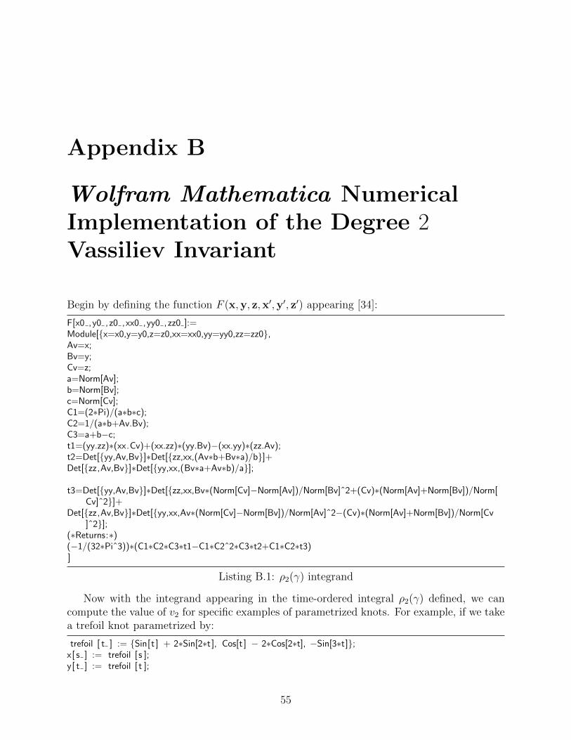
Appendix B

Wolfram Mathematica NumericalImplementation of the Degree 2Vassiliev Invariant

Begin by defining the function F (x,y, z,x′,y′, z′) appearing [34]:

F[x0 ,y0 ,z0 ,xx0 ,yy0 , zz0 ]:=Module[x=x0,y=y0,z=z0,xx=xx0,yy=yy0,zz=zz0,Av=x;Bv=y;Cv=z;a=Norm[Av];b=Norm[Bv];c=Norm[Cv];C1=(2∗Pi)/(a∗b∗c);C2=1/(a∗b+Av.Bv);C3=a+b−c;t1=(yy.zz)∗(xx.Cv)+(xx.zz)∗(yy.Bv)−(xx.yy)∗(zz.Av);t2=Det[yy,Av,Bv]∗Det[zz,xx,(Av∗b+Bv∗a)/b]+Det[zz,Av,Bv]∗Det[yy,xx,(Bv∗a+Av∗b)/a];

t3=Det[yy,Av,Bv]∗Det[zz,xx,Bv∗(Norm[Cv]−Norm[Av])/Norm[Bv]ˆ2+(Cv)∗(Norm[Av]+Norm[Bv])/Norm[Cv]ˆ2]+

Det[zz,Av,Bv]∗Det[yy,xx,Av∗(Norm[Cv]−Norm[Bv])/Norm[Av]ˆ2−(Cv)∗(Norm[Av]+Norm[Bv])/Norm[Cv]ˆ2];

(∗Returns:∗)(−1/(32∗Piˆ3))∗(C1∗C2∗C3∗t1−C1∗C2ˆ2∗C3∗t2+C1∗C2∗t3)]

Listing B.1: ρ2(γ) integrand

Now with the integrand appearing in the time-ordered integral ρ2(γ) defined, we cancompute the value of v2 for specific examples of parametrized knots. For example, if we takea trefoil knot parametrized by:

trefoil [ t ] := Sin[t ] + 2∗Sin[2∗t ], Cos[t ] − 2∗Cos[2∗t], −Sin[3∗t];x[ s ] := trefoil [ s ];y[ t ] := trefoil [ t ];

55

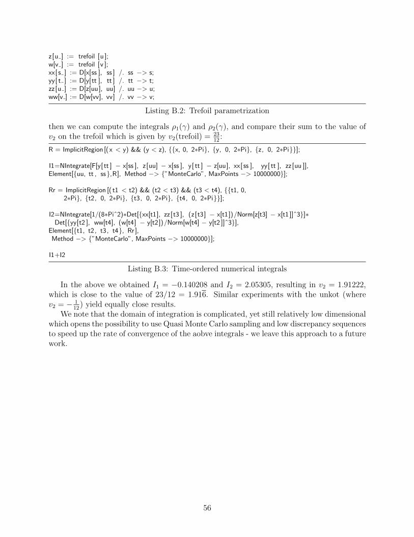
z[u ] := trefoil [u ];w[v ] := trefoil [v ];xx[ s ] := D[x[ss ], ss ] /. ss −> s;yy[ t ] := D[y[tt ], tt ] /. tt −> t;zz[u ] := D[z[uu], uu] /. uu −> u;ww[v ] := D[w[vv], vv] /. vv −> v;

Listing B.2: Trefoil parametrization

then we can compute the integrals ρ1(γ) and ρ2(γ), and compare their sum to the value ofv2 on the trefoil which is given by v2(trefoil) = 23

12:

R = ImplicitRegion [(x < y) && (y < z), x, 0, 2∗Pi, y, 0, 2∗Pi, z, 0, 2∗Pi];

I1=NIntegrate[F[y[ tt ] − x[ss ], z[uu] − x[ss ], y[ tt ] − z[uu], xx[ ss ], yy[ tt ], zz[uu ]],Element[uu, tt , ss,R], Method −> ”MonteCarlo”, MaxPoints −> 10000000];

Rr = ImplicitRegion [( t1 < t2) && (t2 < t3) && (t3 < t4), t1, 0,2∗Pi, t2, 0, 2∗Pi, t3, 0, 2∗Pi, t4, 0, 2∗Pi];

I2=NIntegrate[1/(8∗Piˆ2)∗Det[xx[t1], zz[t3 ], (z[t3] − x[t1])/Norm[z[t3] − x[t1 ]]ˆ3]∗Det[yy[t2 ], ww[t4], (w[t4] − y[t2])/Norm[w[t4] − y[t2 ]]ˆ3],

Element[t1, t2 , t3 , t4, Rr ],Method −> ”MonteCarlo”, MaxPoints −> 10000000];

I1+I2

Listing B.3: Time-ordered numerical integrals

In the above we obtained I1 = −0.140208 and I2 = 2.05305, resulting in v2 = 1.91222,which is close to the value of 23/12 = 1.916. Similar experiments with the unkot (wherev2 = − 1

12) yield equally close results.

We note that the domain of integration is complicated, yet still relatively low dimensionalwhich opens the possibility to use Quasi Monte Carlo sampling and low discrepancy sequencesto speed up the rate of convergence of the aobve integrals - we leave this approach to a futurework.

56

References

[1] Colin Adams, Thomas Crawford, Benjamin DeMeo, Michael Landry, Alex Lin, Mur-phykate Montee, Seojung Park, Saraswathi Venkatesh, and Farrah Yhee. Knot projec-tions with a single multi-crossing. Journal of Knot Theory and Its Ramifications, 24,08 2012.

[2] Sotero Alvarado, Jorge Alberto Calvo, and Kenneth C. Millett. The generation ofrandom equilateral polygons. J. Stat. Phys., 143(1):102–138, 2011. Supplementarymaterial available online.

[3] Z. Arai. A rigorous numerical algorithm for computing the linking number of links.Nonlinear Theory and Its Applications, IEICE, 4:104–110, 2013.

[4] J. Arsuaga, T. Blackstone, Y. Diao, K. Hinson, E. Karadayi, and M. Saito. Samplinglarge random knots in a confined space. J. Phys. A, 40(39):11697–11711, 2007.

[5] Dror Bar-Natan. On the vassiliev knot invariants. Topology, 34(2):423 – 472, 1995.

[6] J. Binet. Memoire sur un systeme du formules analytiques, et leur application a desconsiderations geometriques. J. l’Ecole Polytechnique, 9:280–354, 1813.

[7] Raoul Bott and Clifford Taubes. On the selflinking of knots. Journal of MathematicalPhysics, 35(10):5247–5287, 1994.

[8] Jason Cantarella, Tetsuo Deguchi, and Clayton Shonkwiler. Probability theory of ran-dom polygons from the quaternionic viewpoint. Comm. Pure Appl. Math., 67(10):1658–1699, 2014.

[9] Jason Cantarella, Alexander Y Grosberg, Robert B. Kusner, and Clayton Shonkwiler.The expected total curvature of random polygons. American Journal of Mathematics,137(2):411–438, 2015.

[10] A. Cauchy. Memoire sur les fonctions qui ne peuvent obtenir que deux valeurs egaleset de signes contraires par suite des transpositions operees entre les variables qu’ellesrenferment. J. l’Ecole Polytechnique, 10:29–112, 1815.

[11] Cauchy-Binet Formula. Cauchy-binet formula — Wikipedia, the free encyclopedia.Available at https://en.wikipedia.org/wiki/Cauchy-Binet_formula, 2018. [On-line; accessed 31-December-2018].

57

https://en.wikipedia.org/wiki/Cauchy-Binet_formula

REFERENCES

[12] Moshe Cohen and Sunder Ram Krishnan. Random knots using chebyshev billiard tablediagrams. Topology and its Applications, 194, 05 2015.

[13] Marc Culler, Nathan M. Dunfield, and Jeffrey R. Weeks. SnapPy, a computer programfor studying the topology of 3-manifolds. Available at http://snappy.computop.org.

[14] Y. Diao, A. Dobay, and A. Stasiak. The average inter-crossing number of equilateralrandom walks and polygons. J. Phys. A, 38(35):7601–7616, 2005.

[15] B. Duplantier. Linking numbers, contacts, and mutual inductances of a random set ofclosed curves. Comm. Math. Phys., 82(1):41–68, 1981/82.

[16] Chaim Even-Zohar, Joel Hass, Nati Linial, and Tahl Nowik. Invariants of random knotsand links. Discrete & Computational Geometry, 56, 11 2014.

[17] Chaim Even-Zohar, Joel Hass, Nati Linial, and Tahl Nowik. The distribution of knotsin the petaluma model. Algebraic & Geometric Topology, 18, 06 2017.

[18] Istvan Fary. Sur la courbure totale d’une courbe gauche faisant un nœud. Bull. Soc.Math. France, 77:128–138, 1949.

[19] Franco Ferrari and Yani Zhao. Monte Carlo Computation of the Vassiliev knot invariantof degree 2 in the integral representation. arXiv e-prints, page arXiv:1401.1154, Jan2014.

[20] Eric L. Grinberg and Boris Rubin. Radon inversion on Grassmannians via Garding-Gindikin fractional integrals. Ann. of Math. (2), 159(2):783–817, 2004.

[21] E. Guadagnini, M. Martellini, and M. Mintchev. Braids and quantum group symmetryin chern-simons theory. Nuclear Physics B, 336(3):581 – 609, 1990.

[22] Wolfram Research Inc. Mathematica 9, 2012, Champaign, Illinois.

[23] M. Kontsevich. Vassiliev’s knot invariants. Adv. Soviet Math, 16:137–150, 1993.

[24] Xiao-Song Lin and Zhenghan Wang. Integral geometry of plane curves and knot invari-ants. J. Differential Geom., 44(1):74–95, 1996.

[25] J. W. Milnor. On the total curvature of knots. Ann. of Math. (2), 52:248–257, 1950.

[26] Travis Oliphant. NumPy: A guide to NumPy. USA: Trelgol Publishing, 2006–. [Online;accessed June 18, 2019].

[27] Guido Rossum. Python reference manual. Technical report, Amsterdam, The Nether-lands, The Netherlands, 1995.

[28] Clayton Shonkwiler and David Shea Vela-Vick. Higher-dimensional linking integrals.Proc. Amer. Math. Soc., 139(4):1511–1519, 2011.

[29] John M. Sullivan. Curves of finite total curvature. In Discrete differential geometry,volume 38 of Oberwolfach Semin., pages 137–161. Birkhauser, Basel, 2008.

58

http://snappy.computop.org

REFERENCES

[30] Dylan P. Thurston. Integral expressions for the vassiliev knot invariants, 1999.

[31] V Vassiliev. Cohomology of knot spaces, pages 23–70. 12 1990.

[32] V Vassiliev. Complements of discriminants of smooth maps: topology and applications.transl. from the russian by b. goldfarb. transl. ed. by s. gelfand. 06 2019.

[33] Genkai Zhang. Radon transform on real, complex, and quaternionic Grassmannians.Duke Math. J., 138(1):137–160, 2007.

[34] Yani Zhao and Franco Ferrari. A study of polymer knots using a simple knot invariantconsisting of multiple contour integrals. Journal of Statistical Mechanics: Theory andExperiment, 2013, 06 2013.

59

knots and links from random projection - arxiv · knots and links from random projections by...

Documents