kohavi solution manual
TRANSCRIPT

Solutions for the End-of-the-Chapter Problems in
Switching and Finite Automata Theory, 3rd Ed.
Zvi Kohavi and Niraj K. Jha
Chapter 1
1.2.
(a) (16)10 = (100)4
(b) (292)10 = (1204)6
1.4.
(a) Number systems with base b ≥ 7.
(b) Base b = 8.
1.5. The missing number is (31)5. The series of integers represents number (16)10 in different number
systems.
1.7.
(a) In a positively weighted code, the only way to represent decimal integer 1 is by a 1, and the only
way to represent decimal 2 is either by a 2 or by a sum of 1 + 1. Clearly, decimal 9 can be expressed
only if the sum of the weights is equal to or larger than 9.
(b)
5211* 53214311* 63215311 73216311 44214221* 54215221 64216221 74213321* 84214321
* denotes a self-complementing code. The above list exhausts all the combinations of positive weights
that can be a basis for a code.
1.8.
(a) If the sum of the weights is larger than 9, then the complement of zero will be w1 +w2 +w3 +w4 > 9.
If the sum is smaller than 9, then it is not a valid code.
1

(b) 751 − 4; 832 − 4; 652 − 4.
1.9.
(a) From the map to below, it is evident that the code can be completed by adding the sequence of code
words: 101, 100, 110, 010.
xyz 00 01 11 10
1
0
(b) This code cannot be completed, since 001 is not adjacent to either 100 or 110.
xyz 00 01 11 10
1
0
(c) This code can be completed by adding the sequence of code words: 011, 001, 101, 100.
xyz 00 01 11 10
1
0
(d) This code can be completed by adding code words: 1110, 1100, 1000, 1001, 0001, 0011, 0111, 0110,
0010.
1.13.
(a)
(i) A, C, and D detect single errors.
(ii) C and D detect double errors.
(iii) A and D detect triple errors.
(iv) C and D correct single errors.
(v) None of the codes can correct double errors.
(vi) D corrects single and detects double errors.
(b) Four words: 1101, 0111, 1011, 1110. This set is unique.
2
Chapter 2
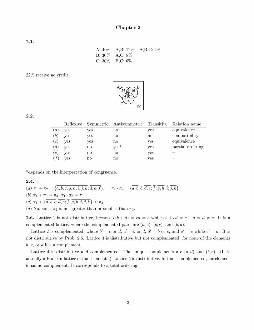
2.1.
A: 40% A,B: 12% A,B,C: 4%B: 30% A,C: 8%C: 30% B,C: 6%
22% receive no credit.
A B
C
24 168
4 4 220
22
2.2.
Reflexive Symmetric Antisymmetric Transitive Relation name
(a) yes yes no yes equivalence(b) yes yes no no compatibility(c) yes yes no yes equivalence(d) yes no yes* yes partial ordering(e) yes no no yes –(f) yes no no yes –
*depends on the interpretation of congruence.
2.4.
(a) π1 + π2 = {a, b, c, g, h, i, j, k ; d, e, f}, π1 · π2 = {a, b; c; d, e; f ; g, h; i; j, k}(b) π1 + π3 = π3, π1 · π3 = π1
(c) π1 < {a, b, c; d, e; f ; g, h, i, j, k} < π3
(d) No, since π2 is not greater than or smaller than π3.
2.6. Lattice 1 is not distributive, because c(b + d) = ca = c while cb + cd = e + d = d 6= c. It is a
complemented lattice, where the complemented pairs are (a, e), (b, c), and (b, d).
Lattice 2 is complemented, where b′ = c or d, c′ = b or d, d′ = b or c, and a′ = e while e′ = a. It is
not distributive by Prob. 2.5. Lattice 3 is distributive but not complemented, for none of the elements
b, c, or d has a complement.
Lattice 4 is distributive and complemented. The unique complements are (a, d) and (b, c). (It is
actually a Boolean lattice of four elements.) Lattice 5 is distributive, but not complemented, for element
b has no complement. It corresponds to a total ordering.
3

Chapter 3
3.3.
(a) x′ + y′ + xyz′ = x′ + y′ + xz′ = x′ + y′ + z′
(b) (x′ + xyz′) + (x′ + xyz′)(x + x′y′z) = x′ + xyz′ = x′ + yz′
(c) xy + wxyz′ + x′y = y(x + wxz′ + x′) = y
(d)a + a′b + a′b′c + a′b′c′d + · · · = a + a′(b + b′c + b′c′d + · · ·)
= a + (b + b′c + b′c′d + · · ·)= a + b + b′(c + c′d + · · ·)= a + b + c + · · ·
(e) xy + y′z′ + wxz′ = xy + y′z′ (by 3.19)
(f) w′x′ + x′y′ + w′z′ + yz = x′y′ + w′z′ + yz (by 3.19)
3.5.
(a) Yes, (b) Yes, (c) Yes, (d) No.
3.7.
A′ + AB = 0 ⇒ A′ + B = 0 ⇒ A = 1, B = 0
AB = AC ⇒ 1 · 0 = 1 · C ⇒ C = 0
AB + AC ′ + CD = C ′D ⇒ 0 + 1 + 0 = D ⇒ D = 1
3.8. Add w′x + yz′ to both sides and simplify.
3.13.
(a) f ′(x1, x2, . . . , xn, 0, 1,+, ·) = f(x′
1, x′
2, . . . , x′
n, 1, 0, ·,+)
f ′(x′
1, x′
2, . . . , x′
n, 1, 0,+, ·) = f(x1, x2, . . . , xn, 0, 1, ·,+) = fd(x1, x2, . . . , xn)
(b) There are two distinct self-dual functions of three variables.
f1 = xy + xz + yz
f2 = xyz + x′y′z + x′yz′ + xy′z′
(c) A self-dual function g of three variables can be found by selecting a function f of two (or three)
variables and a variable A which is not (or is) a variable in f , and substituting to g = Af + A′fd. For
example,
f = xy + x′y′ then fd = (x + y)(x′ + y′)
g = z(xy + x′y′) + z′(x + y)(x′ + y′)
= xyz + x′y′z + xy′z′ + x′yz′ = f2
4

Similarly, if we select f = x + y, we obtain function f1 above.
3.14.
(a) f(x, x, y) = x′y′ = NOR, which is universal.
(b)
f(x, 1) = x′
f(x′, y) = xy
These together are functionally complete.
3.15. All are true except (e), since
1 ⊕ (0 + 1) = 0 6= (1 ⊕ 0) + (1 ⊕ 1) = 1
3.16.
(a)
f(0, 0) = a0 = b0 = c0
f(0, 1) = a1 = b0 ⊕ b1 = c1
f(1, 0) = a2 = b0 ⊕ b2 = c2
f(1, 1) = a3 = b0 ⊕ b1 ⊕ b2 ⊕ b3 = c3
Solving explicitly for the b’s and c’s
b0 = a0
b1 = a0 ⊕ a1
b2 = a0 ⊕ a2
b3 = a0 ⊕ a1 ⊕ a2 ⊕ a3
c0 = a0
c1 = a1
c2 = a2
c3 = a3
(b) The proof follows from the fact that in the canonical sum-of-products form, at any time only one
minterm assumes value 1.
3.20.
f(A,B,C,D,E) = (A + B + E)(C)(A + D)(B + C)(D + E) = ACD + ACE + BCD + CDE
Clearly “C” is the essential executive.
3.21.
xy′z′ + y′z + w′xyz + wxy + w′xyz′ = x + y′z
5

Married or a female under 25.
3.24. Element a must have a complement a′, such that a + a′ = 1. If a′ = 0, then a = 1 (since 1′ = 0),
which is contradictory to the initial assumption that a, 0, and 1 are distinct elements. Similar reasoning
shows that a′ 6= 1. Now suppose a′ = a. However, then a + a′ = a + a = a 6= 1.
3.25.
(a) a + a′b = (a + a′)(a + b) = 1 · (a + b) = a + b
(b) b = b + aa′ = (b + a)(b + a′) = (c + a)(c + a′) = c + aa′ = c
(c)
b = aa′ + b = (a + b)(a′ + b) = (a + c)(a′ + b) = aa′ + a′c + ab + bc
= a′c + ac + bc + c(a′ + a + b) = c
3.26. The (unique) complementary elements are: (30,1), (15,2), (10,3), (6,5)
30
1015 6
23 5
1
Defining a + b ∼= lub(a, b) and a · b ∼= glb(a, b), it is fairly easy to show that this is a lattice and is
distributive. Also, since the lattice is complemented, it is a Boolean algebra.
6
Chapter 4
4.1
(a) f1 = x′ + w′z′ (unique)
(b) f2 = x′y′z′ + w′y′z + xyz + wyz′ or f2 = w′x′y′ + w′xz + wxy + wx′z′
(c) f3 = x′z′ + w′z′ + y′z′ + w′xy′ (unique)
4.2.
(a) MSP = x′z′ + w′yz + wx′y′ (unique)
MPS = (w + y + z′)(w′ + y′ + z′)(x′ + z)(w′ + x′) or (w + y + z′)(w′ + y′ + z′)(x′ + z)(x′ + y) (two
minimal forms)
(b) f = w′x′z′ + xy′z′ + x′y′z + xyz (unique)
4.4.
f =∑
(4, 10, 11, 13) +∑
φ
(0, 2, 5, 15)
= wx′y + wxz + w′xy′
There are four minimal forms.
4.5.
(a) f3 = f1 · f2 =∑
(4) +∑
φ(8, 9) (four functions)
(b) f4 = f1 + f2 =∑
(0, 1, 2, 3, 4, 5, 7, 8, 9, 10, 11, 15) +∑
φ(6, 12)
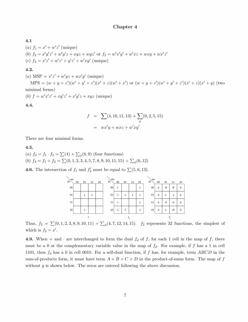
4.6. The intersection of f1 and f ′
2 must be equal to∑
(5, 6, 13).
1 1
1
1
00 01 11 10
00
01
11
10
wxyz
1
f2
1
1 1
1
00 01 11 10
00
01
11
10
wxyz
1
f
1
1 1
1
00 01 11 10
00
01
11
10
wxyz
1
f1
11
0
0
0
00
0
0
0
Thus, f2 =∑
(0, 1, 2, 3, 8, 9, 10, 11) +∑
φ(4, 7, 12, 14, 15). f2 represents 32 functions, the simplest of
which is f2 = x′.
4.9. When + and · are interchanged to form the dual fd of f , for each 1 cell in the map of f , there
must be a 0 at the complementary variable value in the map of fd. For example, if f has a 1 in cell
1101, then fd has a 0 in cell 0010. For a self-dual function, if f has, for example, term ABCD in the
sum-of-products form, it must have term A + B + C + D in the product-of-sums form. The map of f
without g is shown below. The zeros are entered following the above discussion.
7

1
0
0
1
1 1
0
00 01 11 10
00
01
11
10
ABCD
1
01
00
The two pairs of cells connected by arrows can be arbitrarily filled so long as one end of an arrow
points to a 1 and the other end to a 0. Two possible minimal sum-of-products expressions are:
f = AB + BD + BC + ACD
f = CD + A′D + BD + A′BC
4.13.
1
1
1
1
1
1
1
1
1
00 01 11 10
T = yz + w z + x y
00
01
11
10
wxyz
1
1
Essential prime implicantsand unique minimum cover.
1
1
1
1
1
1
1
1
1
00 01 11 10
00
01
11
10
wxyz
1
1
Nonessential primeimplicants.
4.14.
(a) Essential prime implicants: {w′xy′, wxy,wx′y′}Non-essential prime implicants: {w′z, x′z, yz}
(b) T = w′xy′ + wxy + wx′y′+ {any two of (w′z, x′z, yz)}.
4.15.
(a) (i)∑
(5, 6, 7, 9, 10, 11, 13, 14)
(ii)∑
(0, 3, 5, 6, 9, 10, 12, 15)
(b) (i)∑
(5, 6, 7, 9, 10, 11, 12, 13, 14)
(ii)∑
(5, 6, 7, 9, 10, 11, 13, 14, 15)
(c)∑
(0, 4, 5, 13, 15)
(d)∑
(0, 3, 6, 7, 8, 9, 13, 14)
4.16.
(a) False. See, for example, function∑
(3, 4, 6, 7).
(b) False. See, for example, Problem 4.2(a).
(c) True, for it implies that all the prime implicants are essential and, thus, f is represented uniquely
by the sum of the essential prime implicants.
8

(d) True. Take all prime implicants except p, eliminate all the redundant ones; the sum of the remaining
prime implicants is an irredundant cover.
(e) False. See the following counter-example.
1
1
1
1
1
1
000 001 011 010
00
01
11
10
vwxyz
1
1
1
1
1
1
1
1
1
110 111 101 100
1
4.17.
(a)
1
1
1 1
1
00 01 11 10
00
01
11
10
ABCD
1
1
1
(b) To prove existence of such a function is a simple extension of (a); it can be represented as a sum
of 2n−1 product terms. Adding another true cell can only create an adjacency which will reduce the
number of cubes necessary for a cover.
(c) From the above arguments, clearly n2n−1 is the necessary bound.
4.18.
(a) Such a function has(
nk
)
=n!
k!(n − k)!
1’s, of which no two are adjacent. Thus, the number of prime implicants equals the number of 1’s. All
prime implicants are essential.
(b) Each of the cells of the function from part (a) will still be contained in a distinct prime implicant,
although it may not be an essential prime implicant. Each cube now covers 2n−k cells, and there are
(
nk
)
=n!
k!(n − k)!
such cubes.
4.19.
(a) T is irredundant and depends on D. Thus, no expression for T can be independent of D.
9
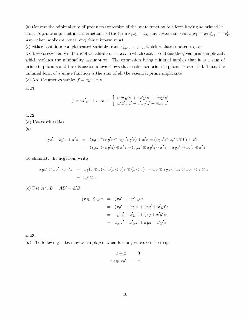
(b) Convert the minimal sum-of-products expression of the unate function to a form having no primed lit-
erals. A prime implicant in this function is of the form x1x2 · · · xk, and covers minterm x1x2 · · · xkx′
k+1 · · · x′
n.
Any other implicant containing this minterm must:
(i) either contain a complemented variable from x′
k+1, · · · , x′
n, which violates unateness, or
(ii) be expressed only in terms of variables x1, · · · , xk, in which case, it contains the given prime implicant,
which violates the minimality assumption. The expression being minimal implies that it is a sum of
prime implicants and the discussion above shows that each such prime implicant is essential. Thus, the
minimal form of a unate function is the sum of all the essential prime implicants.
(c) No. Counter-example: f = xy + x′z
4.21.
f = vx′yz + vwxz +
{
v′w′y′z′ + vx′y′z′ + wxy′z′
w′x′y′z′ + v′xy′z′ + vwy′z′
4.22.
(a) Use truth tables.
(b)
xyz′ + xy′z + x′z = (xyz′ ⊕ xy′z ⊕ xyz′xy′z) + x′z = (xyz′ ⊕ xy′z ⊕ 0) + x′z
= (xyz′ ⊕ xy′z) ⊕ x′z ⊕ (xyz′ ⊕ xy′z) · x′z = xyz′ ⊕ xy′z ⊕ x′z
To eliminate the negation, write
xyz′ ⊕ xy′z ⊕ x′z = xy(1 ⊕ z) ⊕ x(1 ⊕ y)z ⊕ (1 ⊕ x)z = xy ⊕ xyz ⊕ xz ⊕ xyz ⊕ z ⊕ xz
= xy ⊕ z
(c) Use A ⊕ B = AB′ + A′B.
(x ⊕ y) ⊕ z = (xy′ + x′y) ⊕ z
= (xy′ + x′y)z′ + (xy′ + x′y)′z
= xy′z′ + x′yz′ + (xy + x′y′)z
= xy′z′ + x′yz′ + xyz + x′y′z
4.23.
(a) The following rules may be employed when forming cubes on the map:
x ⊕ x = 0
xy ⊕ xy′ = x
10
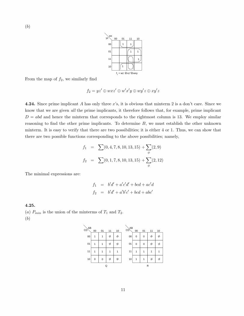
(b)
1
1
1
1
1
00 01 11 10
f1 = wz + xz + wxy
00
01
11
10
wxyz
1
From the map of f2, we similarly find
f2 = yz′ ⊕ wxz′ ⊕ w′x′y ⊕ wy′z ⊕ xy′z
4.24. Since prime implicant A has only three x’s, it is obvious that minterm 2 is a don’t care. Since we
know that we are given all the prime implicants, it therefore follows that, for example, prime implicant
D = abd and hence the minterm that corresponds to the rightmost column is 13. We employ similar
reasoning to find the other prime implicants. To determine B, we must establish the other unknown
minterm. It is easy to verify that there are two possibilities; it is either 4 or 1. Thus, we can show that
there are two possible functions corresponding to the above possibilities; namely,
f1 =∑
(0, 4, 7, 8, 10, 13, 15) +∑
φ
(2, 9)
f2 =∑
(0, 1, 7, 8, 10, 13, 15) +∑
φ
(2, 12)
The minimal expressions are:
f1 = b′d′ + a′c′d′ + bcd + ac′d
f2 = b′d′ + a′b′c′ + bcd + abc′
4.25.
(a) Pmin is the union of the minterms of T1 and T2.
(b)
1
1 1
1
1
1
1
00 01 11 10
00
01
11
10
ABCD
1
Q
1 1 1
00 01 11 10
00
01
11
10
ABCD
1
R
1
1
0
0
0 0
0
0
11
(c)
0
1
0
0
0
1
0
00 01 11 10
00
01
11
10
ABCD
0
Pmax
0
00
00 01 11 10
00
01
11
10
ABCD
1
Q
1
0
1
1
0 0
1
1
01
0 0
0
00 01 11 10
00
01
11
10
ABCD
R
1
0
00
000
00
00
00
00
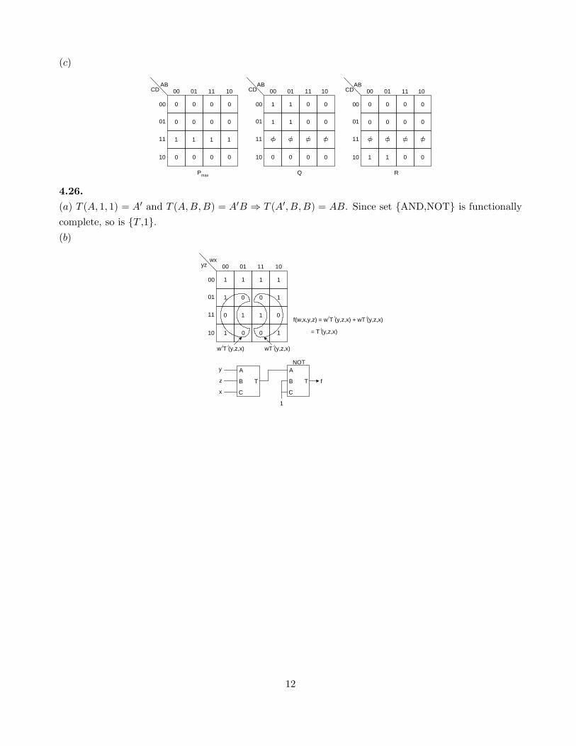
4.26.
(a) T (A, 1, 1) = A′ and T (A,B,B) = A′B ⇒ T (A′, B,B) = AB. Since set {AND,NOT} is functionally
complete, so is {T ,1}.(b)
1
0
1
1
0
00 01 11 10
00
01
11
10
wxyz
0
w T (y,z,x)
11
1 0 10
10
11
wT (y,z,x)
f(w,x,y,z) = w T (y,z,x) + wT (y,z,x)
= T (y,z,x)
y
x
z T
A
B
C
T
A
B
C
1
f
NOT
12
Chapter 5
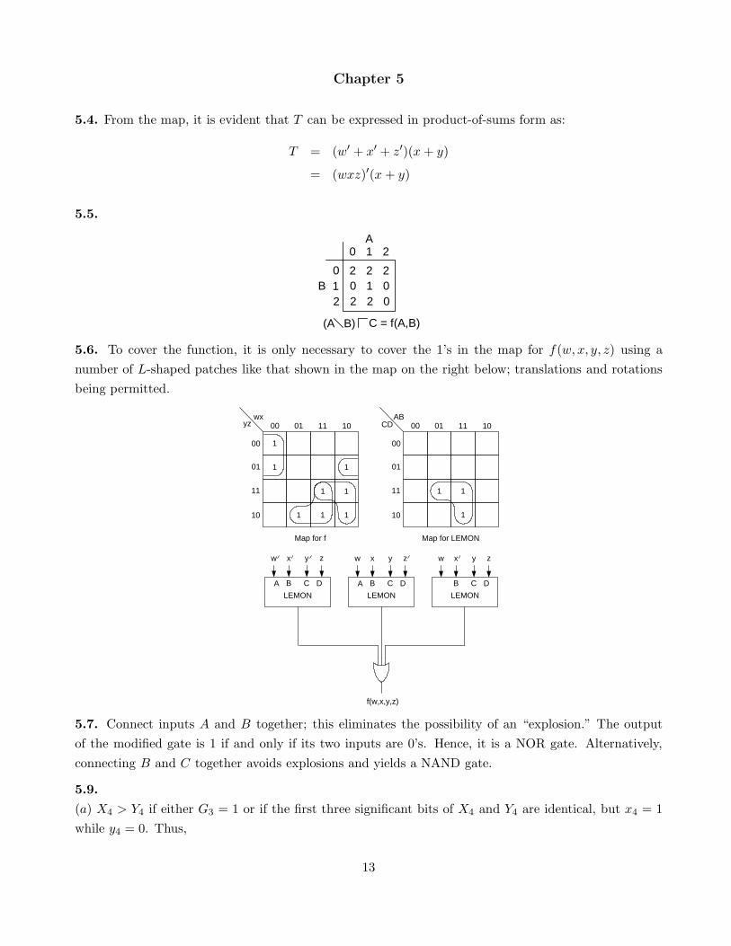
5.4. From the map, it is evident that T can be expressed in product-of-sums form as:
T = (w′ + x′ + z′)(x + y)
= (wxz)′(x + y)
5.5.
B) C = f(A,B)
A
B
0 1 2
012
2 2 2
2 2 00 1 0
(A
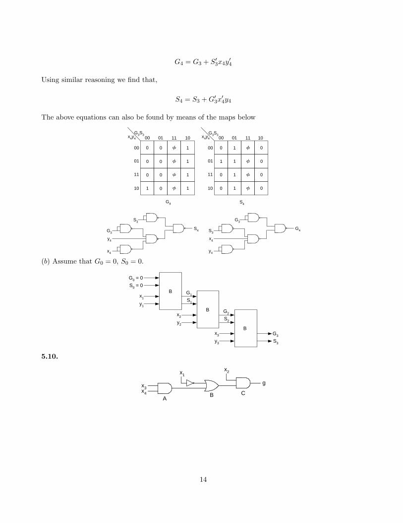
5.6. To cover the function, it is only necessary to cover the 1’s in the map for f(w, x, y, z) using a
number of L-shaped patches like that shown in the map on the right below; translations and rotations
being permitted.
1 1
1
111
1
00 01 11 10
00
01
11
10
wxyz
1
Map for f
1
1
1
00 01 11 10
00
01
11
10
ABCD
Map for LEMON
f(w,x,y,z)
w
A
zyx
LEMON
B C D
w
A
zyx
B C D
LEMON
zyx
B C D
LEMON
w
5.7. Connect inputs A and B together; this eliminates the possibility of an “explosion.” The output
of the modified gate is 1 if and only if its two inputs are 0’s. Hence, it is a NOR gate. Alternatively,
connecting B and C together avoids explosions and yields a NAND gate.
5.9.
(a) X4 > Y4 if either G3 = 1 or if the first three significant bits of X4 and Y4 are identical, but x4 = 1
while y4 = 0. Thus,
13
G4 = G3 + S′
3x4y′
4
Using similar reasoning we find that,
S4 = S3 + G′
3x′
4y4
The above equations can also be found by means of the maps below
1
0
0
1
1
1 1
1
00 01 11 10
00
01
11
10
G3S3x4y4
0
S4
1
1
0
00 01 11 10
00
01
11
10
1
S4
010
0
0
G3S3x4y4
0 0
0
0
0
0
G3
x4
y4
S3
G4S3
y4
x4
G3
G4
(b) Assume that G0 = 0, S0 = 0.
B
G0 = 0
y1
S1
G1x1
S0 = 0
By2
x2
y3
x3
G2
S2
G3
S3
B
5.10.
AB
x3g
x4
x1
C
x2
14
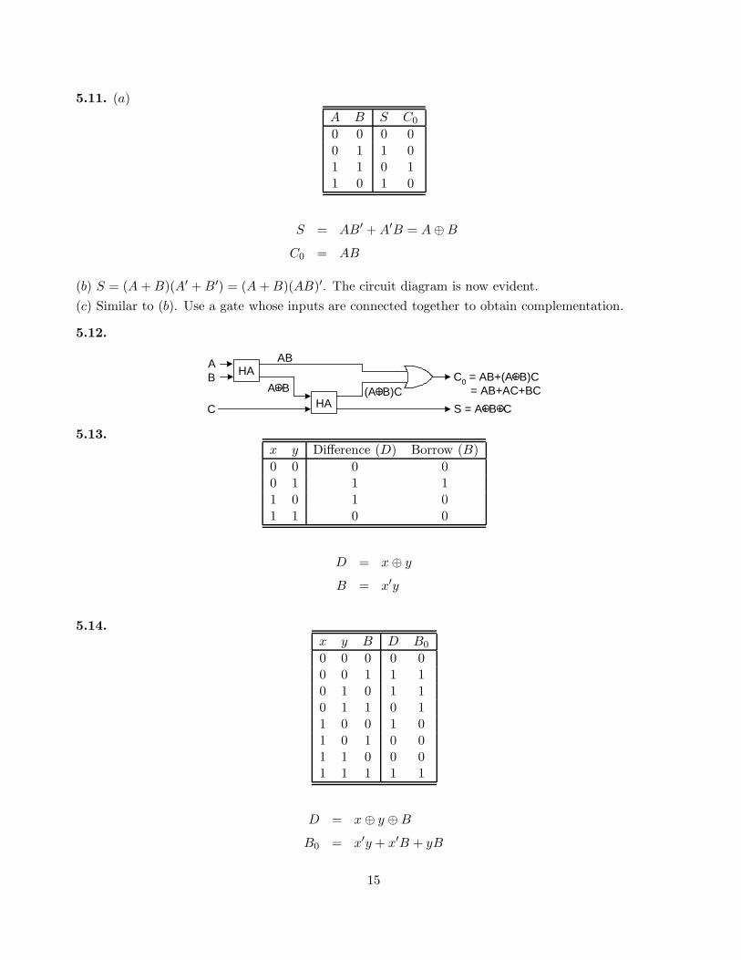
5.11. (a)
A B S C0
0 0 0 00 1 1 01 1 0 11 0 1 0
S = AB′ + A′B = A ⊕ B
C0 = AB
(b) S = (A + B)(A′ + B′) = (A + B)(AB)′. The circuit diagram is now evident.
(c) Similar to (b). Use a gate whose inputs are connected together to obtain complementation.
5.12.
BHA C0 = AB+(A+B)C
= AB+AC+BC
A
C
AB
HAA+B (A+B)C
S = A+B+C
5.13.x y Difference (D) Borrow (B)
0 0 0 00 1 1 11 0 1 01 1 0 0
D = x ⊕ y
B = x′y
5.14.x y B D B0
0 0 0 0 00 0 1 1 10 1 0 1 10 1 1 0 11 0 0 1 01 0 1 0 01 1 0 0 01 1 1 1 1
D = x ⊕ y ⊕ B
B0 = x′y + x′B + yB
15

5.15. The circuit is a NAND realization of a full adder.
5.17. A straightforward solution by means of a truth table. Let A = a1a0, B = b1b0 and C = A · B =
c3c2c1c0.
a1 a0 b1 b0 c3 c2 c1 c0
0 0 0 0 0 0 0 00 0 0 1 0 0 0 00 0 1 0 0 0 0 00 0 1 1 0 0 0 00 1 0 0 0 0 0 00 1 0 1 0 0 0 10 1 1 0 0 0 1 00 1 1 1 0 0 1 11 0 0 0 0 0 0 01 0 0 1 0 0 1 01 0 1 0 0 1 0 01 0 1 1 0 1 1 01 1 0 0 0 0 0 01 1 0 1 0 0 1 11 1 1 0 0 1 1 01 1 1 1 1 0 0 1
c0 = a0b0
c1 = a1b0b′
1 + a0b′
0b1 + a′0a1b0 + a0a′
1b1
c2 = a′0a1b1 + a1b′
0b1
c3 = a0a1b0b1
A simpler solution is obtained by observing that
c0
a1a0
+
b1b0
a0b0a1b0
a0b1a1b1
c1c2c3
The ci’s can now be realized by means of half adders as follows:
16

a1
HA
b1 a0
HA
b1 a1 b0 b0a0
c1c3 c2 c0
C0C0
SS
5.19. Since the distance between A and B is 4, one code word cannot be permuted to the other due
to noise in only two bits. In the map below, the minterms designated A correspond to the code word
A and to all other words which are at a distance of 1 from A. Consequently, when any of these words
is received, it implies that A has been transmitted. (Note that all these minterms are at a distance 3
from B and, thus, cannot correspond to B under the two-error assumption.) The equation for A is thus
given by
A = x′
1x′
2x3 + x′
1x′
2x′
4 + x′
1x3x′
4 + x′
2x3x′
4
Similarly, B is given by
B = x1x2x′
3 + x1x2x4 + x2x′
3x4 + x1x′
3x4
The minterms labeled C correspond to output C.
C
B
A
B
B B
C
00 01 11 10
00
01
11
10
x1x2
C
AA
CA
A
C
B
C
x3x4
5.20.
(a)
Tie sets: ac′; ad; abc; b′cd
Cut sets: (a + b′); (a + b + c); (b + c′ + d)
T = (a + b′)(a + b + c)(b + c′ + d)
(b) Let d = 0 and choose values for a, b, and c, such that T = 0; that is, choose a = 0, b = 0, c = 1.
Evidently, T cannot change from 0 to 1, unless a d branch exists and is changed from 0 to 1.
17
(c)
db
a
c
c
b
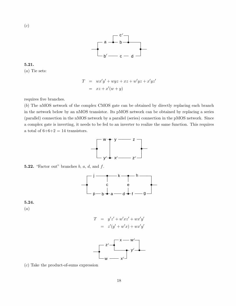
5.21.
(a) Tie sets:
T = wx′y′ + wyz + xz + w′yz + x′yz′
= xz + x′(w + y)
requires five branches.
(b) The nMOS network of the complex CMOS gate can be obtained by directly replacing each branch
in the network below by an nMOS transistor. Its pMOS network can be obtained by replacing a series
(parallel) connection in the nMOS network by a parallel (series) connection in the pMOS network. Since
a complex gate is inverting, it needs to be fed to an inverter to realize the same function. This requires
a total of 6+6+2 = 14 transistors.
y z
z
x
yw
5.22. “Factor out” branches b, a, d, and f .
ap b
k
c
hj
fd
e
g
5.24.
(a)
T = y′z′ + w′xz′ + wx′y′
= z′(y′ + w′x) + wx′y′
w
zw
x
x
y
(c) Take the product-of-sums expression
18
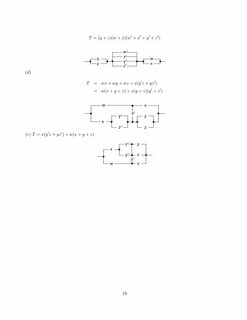
T = (y + z)(w + x)(w′ + x′ + y′ + z′)
z
w
w
z xy x
y
(d)
T = wx + wy + wz + x(y′z + yz′)
= w(x + y + z) + x(y + z)(y′ + z′)
x
x
yx
w
z
y
z
(e) T = x(y′z + yz′) + w(x + y + z)
w
xy
x
z
zy
x
19

Chapter 6
6.1.
(a) No, because of the wwx term
(b) Yes, even though the corresponding sum-of-products expression can be reduced using the consensus
theorem.
(c) No, the sum-of-products expression contains yz and wyz. Since yz contains wyz, this is not an
algebraic factored form.
6.2.
(a)
Algebraic divisors: x + y, x + z, y + z, x + y + z
Boolean divisors: v + w, v + x, v + y, v + z, v + x + y, v + x + z, v + y + z, v + x + y + z
(b) Algebraic divisor x + y + z leads to the best factorization: v + w(x + y + z) with only five literals.
6.3.
Level Kernel Co-kernel
0 y′ + z vw, x′
0 vw + x′ y′, z1 vy′ + vz + x w2 vwy′ + vwz + x′y′ + x′z + wx 1
6.4.
(a)
Cube-literal incidence matrix
Literal
Cube u v w x y z′
wxz′ 0 0 1 1 0 1uwx 1 0 1 1 0 0wyz′ 0 0 1 0 1 1uwy 1 0 1 0 1 0v 0 1 0 0 0 0
20

(b)
Prime rectangles and co-rectangles
Prime rectangle Co-rectangle
({wxz′, uwx}, {w, x}) ({wxz′, uwx}, {u, v, y, z′})({wxz′, wyz′}, {w, z′}) ({wxz′, wyz′}, {u, v, x, y})
({wxz′, uwx,wyz′, uwy}, {w}) ({wxz′, uwx,wyz′, uwy}, {u, v, x, y, z′})({uwx, uwy}, {u,w}) ({uwx, uwy}, {v, x, y, z′})({wyz′, uwy}, {w, y}) ({wyz′, uwy}, {u, v, x, z′})
(c)
Kernels and co-kernels
Kernel Co-kernel
u + z′ wxx + y wz′
xz′ + ux + yz′ + uy wx + y uwu + z′ wy
6.6.
H = x + y
G(H,w, z) = 0 · w′z′ + 1 · w′z + H ′ · wz′ + H · wz
= w′z + H ′wz′ + Hwz
= w′z + H ′wz′ + Hz
6.8.
(a) Consider don’t-care combinations 1, 5, 25, 30 as true combinations (i.e., set them equal to 1). Then
H(v, x, z) =∑
(0, 5, 6) = v′x′z′ + vx′z + vxz′
G(H,w, y) = H ′w′y′ + Hwy′ + Hwy
= H ′w′y′ + Hw
6.9.
(a)
Permuting x and y yields: yxz + yx′z′ + y′xz′ + y′x′z, which is equal to f .
Permuting x and z yields: zyx + zy′x′ + z′yx′ + z′y′x, which is equal to f .
Permuting y and z yields: xzy + xz′y′ + x′zy′ + x′z′y, which is equal to f .
(b) Decomposition:
f1 = yz + y′z′
f = xf1 + x′f ′
1
21

6.10.
(a)
(a) INV. (c) NOR2.(b) NAND2. (d) AOI21.
(e) AOI22. (f) OAI21. (g) OAI22.
6.11.
(a)
wx
yz
vc1
c2
c4
c3
f
(b)
Matches
Node Match
f INVc1 NAND2c2 NAND2c3 NAND2c4 NAND2
Optimum-area network cover: 1+2×4 = 9.
(c) Decomposed subject graph with INVP inserted (ignore the cover shown for now):
w
x
y
z v
c1
c2c4
c3
f
c8
c7
c6
c5
c9
c10
c12
c11
AOI22INV
NOR2
22
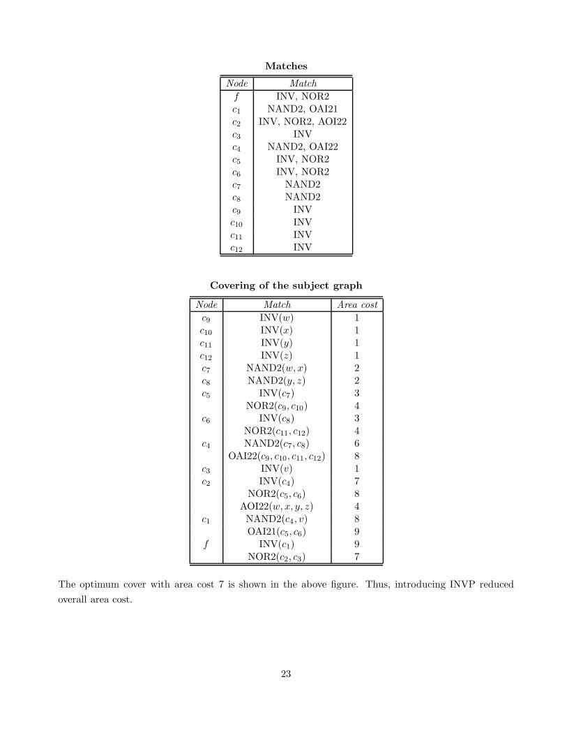
Matches
Node Match
f INV, NOR2c1 NAND2, OAI21c2 INV, NOR2, AOI22c3 INVc4 NAND2, OAI22c5 INV, NOR2c6 INV, NOR2c7 NAND2c8 NAND2c9 INVc10 INVc11 INVc12 INV
Covering of the subject graph
Node Match Area cost
c9 INV(w) 1c10 INV(x) 1c11 INV(y) 1c12 INV(z) 1c7 NAND2(w, x) 2c8 NAND2(y, z) 2c5 INV(c7) 3
NOR2(c9, c10) 4c6 INV(c8) 3
NOR2(c11, c12) 4c4 NAND2(c7, c8) 6
OAI22(c9, c10, c11, c12) 8c3 INV(v) 1c2 INV(c4) 7
NOR2(c5, c6) 8AOI22(w, x, y, z) 4
c1 NAND2(c4, v) 8OAI21(c5, c6) 9
f INV(c1) 9NOR2(c2, c3) 7
The optimum cover with area cost 7 is shown in the above figure. Thus, introducing INVP reduced
overall area cost.
23
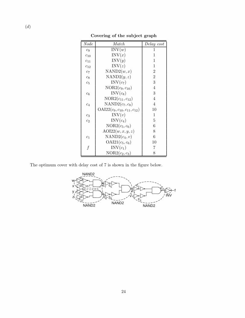
(d)
Covering of the subject graph
Node Match Delay cost
c9 INV(w) 1c10 INV(x) 1c11 INV(y) 1c12 INV(z) 1c7 NAND2(w, x) 2c8 NAND2(y, z) 2c5 INV(c7) 3
NOR2(c9, c10) 4c6 INV(c8) 3
NOR2(c11, c12) 4c4 NAND2(c7, c8) 4
OAI22(c9, c10, c11, c12) 10c3 INV(v) 1c2 INV(c4) 5
NOR2(c5, c6) 6AOI22(w, x, y, z) 8
c1 NAND2(c4, v) 6OAI21(c5, c6) 10
f INV(c1) 7NOR2(c2, c3) 8
The optimum cover with delay cost of 7 is shown in the figure below.
w
x
y
z v
c1
c2
c4
c3
f
c8
c7
c6
c5
c9
c10
c12
c11 INV
NAND2NAND2
NAND2
NAND2
24
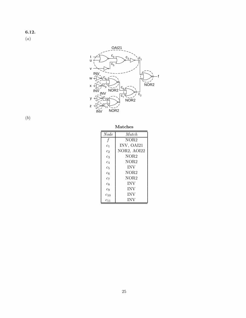
6.12.
(a)
t c1
c2
c3
c7
c6
c5
c4
c9
c8
c10
c11
y
x
w f
v
u
z
NOR2
NOR2
NOR2
NOR2
OAI21
INV
INV
INVINV
(b)
Matches
Node Match
f NOR2c1 INV, OAI21c2 NOR2, AOI22c3 NOR2c4 NOR2c5 INVc6 NOR2c7 NOR2c8 INVc9 INVc10 INVc11 INV
25
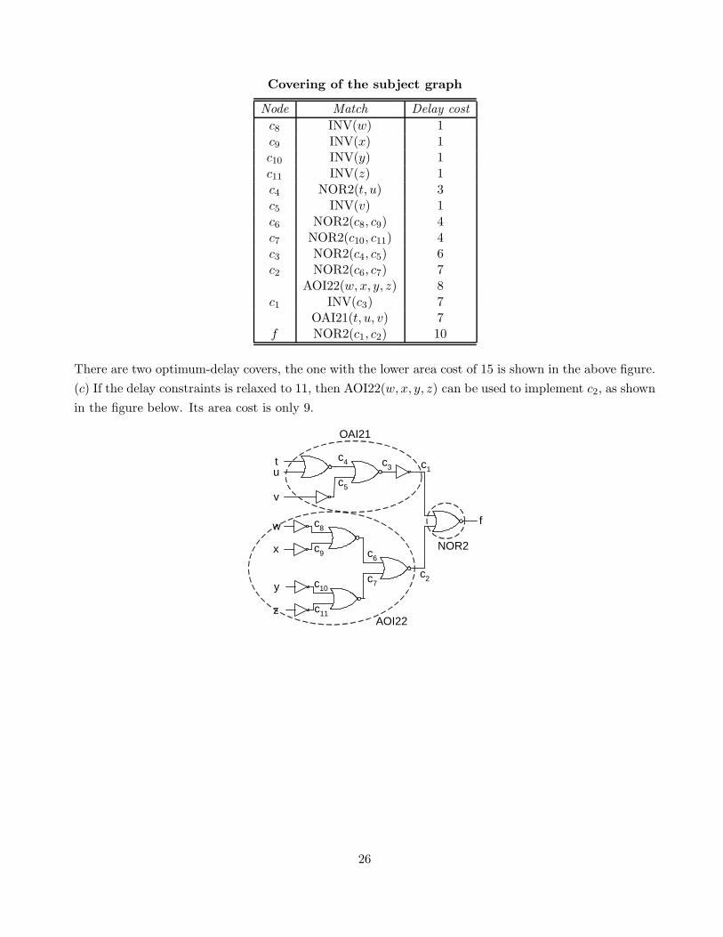
Covering of the subject graph
Node Match Delay cost
c8 INV(w) 1c9 INV(x) 1c10 INV(y) 1c11 INV(z) 1c4 NOR2(t, u) 3c5 INV(v) 1c6 NOR2(c8, c9) 4c7 NOR2(c10, c11) 4c3 NOR2(c4, c5) 6c2 NOR2(c6, c7) 7
AOI22(w, x, y, z) 8c1 INV(c3) 7
OAI21(t, u, v) 7f NOR2(c1, c2) 10
There are two optimum-delay covers, the one with the lower area cost of 15 is shown in the above figure.
(c) If the delay constraints is relaxed to 11, then AOI22(w, x, y, z) can be used to implement c2, as shown
in the figure below. Its area cost is only 9.
t c1
c2
c3
c7
c6
c5
c4
c9
c8
c10
c11
y
x
w f
v
u
z
NOR2
AOI22
OAI21
26

Chapter 7
7.1.
(a) The entries in the map at the left below indicate the weights associated with the corresponding input
combinations. For example, the entry in cell 1001 is −4, since w1x1 + w4x4 = −1− 3 = −4. The weight
associated with each cell can be found by adding the weights of the corresponding row and column. Star
symbol * marks those cells that are associated with weights larger than T = −12 .
1*
2*
-2
-3
2*
4*
0*
-1
-4
00 01 11 10
wixi
00
01
11
10
x1x2
-1
0*
1
1
1
1 1
1
1
00 01 11 10
00
01
11
10
1
1
x3x4
-1
1*
-2
3* 1*
weights
-3
-1
2
x3x4
x1x2weights2 1 -1
Map of function
f(x1, x2, x3, x4) = x2x3 + x3x′
4 + x2x′
4 + x′
1x′
4
(b) Let g be the function realized by the left threshold element, then for f(x1, x2, x3, x4), we obtain the
following maps:
8*
5*
8*
5*
2
3
6*
2
3
00 01 11 10
wixi + 4g(x1,x2,x3,x4)
00
01
11
10
x1x2
6*
4*
11
1
1 1
1
1
00 01 11 10
00
01
11
10
1
1
x3x4
3
4*
5*
5* 3
weights
1
2
1
x3x4
x1x2weights2 4 2
Map of function
1T = 7
2
f(x1, x2, x3, x4) = x′
1x′
2 + x1x2 + x3x4
7.2.
(a) The following inequalities must be satisfied:
w3 > T , w2 > T , w2 + w3 > T , w1 + w2 < T ,
w1 + w2 + w3 > T , w1 < T , w1 + w3 < T , 0 < T
These inequalities are satisfied by the element whose weight-threshold vector is equal to {−2,2,2; 1}.Hence, function f1(x1, x2, x3) is a threshold function.
(b) The inequalities are:
0 > T , w2 > T , w3 < T , w2 + w3 < T
w1 + w2 > T , w1 + w2 + w3 < T , w1 > T , w1 + w3 > T
27

Function f2(x1, x2, x3) is realizable by threshold element {1,−1,−2; −32}.
(c) Among the eight inequalities, we find the following four:
0 > T , w3 < T , w2 < T , w2 + w3 > T
The last three inequalities can only be satisfied if T > 0; but this contradicts the first inequality. Hence,
f3(x1, x2, x3) is not a threshold function.
7.4.
(a) Threshold element {1,1; 12} clearly generates the logical sum of the two other elements.
3*
-1
3*
3*
1
0
4*
1
4*
00 01 11 10
00
01
11
10
x1x2
2
0
1
1
1
1
1
1
00 01 11 10
00
01
11
10
1
1
x3x4
4*
2
5*
1 0
3
2
-1
x3x4
x1x21 2 1
f
1
-1
-2
-2
-1
2*
0
0
1
0
00 01 11 10
00
01
11
10
x1x2
-3
0
x3x4
1
3*
2*
1 -1
-1
-3
-2
2 3 1
Top element Bottom element
+ =
f(x1, x2, x3, x4) = x′
3x4 + x2x′
3 + x2x4 + x1x4
(b) Using the techniques of Sec. 7.2, we obtain
Φ(x1, x2, x3, x4) = f(x1, x2, x′
3, x4) = x3x4 + x2x3 + x2x4 + x1x4
Minimal true vertices: 0011, 0110, 0101, 1001
Maximal false vertices: 1100, 1010, 0001
w3 + w4
w2 + w3
w2 + w4
w1 + w4
>
w1 + w2
w1 + w3
w4
⇒w4 > w1
w3 > w1
w2 > w1
w2 + w3 > w4
w4 > w2
w4 > w3
In other words, w4 > {w2, w3} > w1. Choose w1 = 1, w2 = w3 = 2, and w4 = 3. This choice, in turn,
implies T = 72 . Thus,
VΦ = {1, 2, 2, 3; 7
2}
and
Vf = {1, 2,−2, 3;3
2}
7.5.
(a)
1. Tw
= 0;∑
xi ≥ 0. Hence, f is identically equal to 1.
28
2. Tw
> n;∑
xi ≤ n. Hence, f is identically equal to 0.
3. 0 < Tw≤ n; then f = 1 if p or more variables equal 1 and f = 0 if p− 1 variables or fewer variables
equal 1, where p − 1 < Tw≤ p for p = 0, 1, 2, · · ·.
7.6.
(a) By definition, fd(x1, x2, · · · , xn) = f ′(x′
1, x′
2, · · · , x′
n). Let g(x1, x2, · · · , xn) = f(x′
1, x′
2, · · · , x′
n), then
the weight-threshold vector for g is
Vg = {−w1,−w2, · · · ,−wn; T − (w1 + w2 + · · · + wn)}
Now, since fd = g′, we find
Vfd= {w1, w2, · · · , wn; (w1 + w2 + · · · + wn) − T}
(b) Let V be the weight-threshold vector for f , where V = {w1, w2, · · · , wn; T}. Utilizing the result of
part (a), we find that g = x′
if + xifd equals 1 if and only if xi = 0 and∑
wjxj > T , OR if and only if
xi = 1 and∑
wjxj > (w1 + w2 + · · · + wn) − T .
Establishing, similarly, the conditions for g = 0, we find weight wi of xi, namely
wi = (w1 + w2 + · · · + wn) − 2T =∑
f
wj − 2T
Thus, the weight-threshold vector for g is
Vg = {w1, w2, · · · , wn,∑
f
wj − 2T ; T}
7.7.
(a) In G, for xp = 0, G = f . Thus, Tg = T . When xp = 1,∑
n wi+wp should be larger than T , regardless
of the values of∑
n wi. Define N as the most negative value that∑
n wi can take, then N + wp > T ,
which yields wp > T − N . Choose wp = T − N + 1, then
Vg = {w1, w2, · · · , wn, T − N + 1; T}
Similarly, we can find weight-threshold vector Vh = {w1, w2, · · · , wn, wp; Th} of H, that is
Vh = {w1, w2, · · · , wn,M − T + 1; M + 1}
Note: If xp is a member of set {x1, x2, · · · , xn}, then N and M must be defined, such that the contribution
of wp is excluded.
7.10.
(a) Proof that “common intersection” implies unateness: If the intersection of the prime implicants is
nonzero, then in the set of all prime implicants, each variable appears only in primed or in unprimed
29
form, but not in both, since otherwise the intersection of the prime implicants would contain some pair
xix′
i and would be zero. Also, since f is a sum of prime implicants, it is unate by definition.
Proof that unateness implies “common intersection”: Write f as a sum of all its prime implicants.
Assume that f is positive (negative) in xi and literal x′
i (xi) appears in some prime implicant. By
Problem 7.9, this literal is redundant and the corresponding term is not a prime implicant. However,
this contradicts our initial assumption; hence, each variable appears only in primed or unprimed form
in the set of all prime implicants. This implies that the intersection of the prime implicants is nonzero,
and is an implicant of f which is covered by all the prime implicants.
(b) The proof follows from the above and from Problem 4.19.
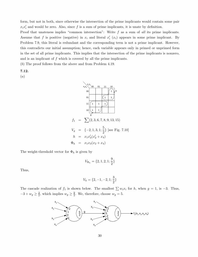
7.12.
(a)
11
1
1
1 1
1
00 01 11 10
00
01
11
10
x1x2
1
g
h
x3x4
f1 =∑
(2, 3, 6, 7, 8, 9, 13, 15)
Vg = {−2, 1, 3, 1;5
2} [see Fig. 7.10]
h = x1x′
3(x′
2 + x4)
Φh = x1x3(x2 + x4)
The weight-threshold vector for Φh is given by
VΦh= {2, 1, 2, 1; 9
2}
Thus,
Vh = {2,−1,−2, 1;3
2}
The cascade realization of f1 is shown below. The smallest∑
wixi for h, when g = 1, is −3. Thus,
−3 + wg ≥ 32 , which implies wg ≥ 9
2 . We, therefore, choose wg = 5.
x3
x2
x1
x4
-2131
52
f1(x1,x2,x3,x4)
x3
x2
x1
x4
2-15
1
32
g
-2
30

(b) f2 =∑
(0, 3, 4, 5, 6, 7, 8, 11, 12, 15)
11
1
1
1
1
1
00 01 11 10
00
01
11
10
x1x2
1g
h
x3x4
1
1
It is easy to verify that g(x1, x2, x3, x4) can be realized by the element with weight-threshold vector
Vg = {−1, 1,−3,−2;−3
2}
Also, since h(x1, x2, x3, x4) = g(x1, x2, x′
3, x′
4), we conclude
Vh = {−1, 1, 3, 2;7
2}
A possible realization of f2 is shown below.
x3
x2
x1
x4
-11-3-2
32
f2(x1,x2,x3,x4)
x3
x2
x1
x4
-115
2
72
g
3
7.13. The implementation is given below.
b
a
ci
1
11 2 s
b
a
ci
1
11 1
b
a
ci
1
11 3
1
1-1 1
co
7.15. The implementation is given below.
M
M M
b
ab s
ci
a
ci
co
31
Chapter 8
8.1.
(a) The vector that activates the fault and sensitizes the path through gates G5 and G8 requires: (i)
c1 = 1 ⇒ x2 = 0 and x3 = 0, (ii) G6 = 0 regardless of whether a fault is present, which implies x4 = 1,
(iii) G7 = 0, which implies G3 = 1 (since x3 = 0), which in turn implies x4 = 0, and (iv) G4 = 0. Thus,
we need to set conflicting requirements on x4, which leads to a contradiction. By the symmetry of the
circuit, it is obvious that an attempt to sensitize the path through gates G6 and G8 will also fail.
(b) Sensitizing both the paths requires: (i) c1 = 1 ⇒ x2 = 0 and x3 = 0, (ii) G4 = 0, which implies
G1 = 1 (since x2 = 0), which in turn implies x1 = x3 = 0, and (iii) G7 = 0, which implies G3 = 1 (since
x3 = 0), which in turn implies x2 = x4 = 0. All these conditions can be satisfied by the test vector
(0,0,0,0).
8.2.
(a) Label the output of the AND gate realizing C ′E as c5 and the output of the OR gate realizing B′+E′
as c6. To detect A′ s-a-0 by D-algorithm, the singular cover will set A′ = D, c5 = 0 and c1 = c2 = D.
Performing backward implication, we get (C,E) = (1,φ) or (φ,0). Performing D-drive on the upper
path with B = 1 and c4 = 0 allows the propagation of D to output f . c4 = 0 can be justified through
backward implication by c6 = 0, which in turn implies (B,E) = (1,1). All of the above values can now
be justified by (A,B,C,E) = (0,1,1,1), which is hence one of the test vectors.
The other test vectors can be obtained by performing the D-drive through the lower path with c6 = 1
(implying (B,E) = (0,φ) or (φ,0)) and c3 = 0. c3 = 0 can be justified by B = 0. The test vectors that
meet all the above conditions are {(0,0,φ,0), (0,0,1,φ)}.Since the two paths have unequal inversion parity emanating from A′ and reconverging at f , we must
ensure that only one of these paths will be sensitized at a time.
(b) We assume that a fault on input B′ is independent of the value of input B; similarly for inputs E′
and E; that is, a fault can occur on just one of these inputs. The faults detected are: s-a-1 on lines A′,
B′, C ′, E′, c1, c3, c4, c5, c6 and f .
8.3.
(a) The key idea is that when F = 0, both inputs of the OR gates can be sensitized simultaneously and,
therefore, both subnetworks can be tested simultaneously. Thus, the number of tests resulting in F = 0
is determined by the subnetwork requiring the larger number of tests, namely,
n0f = max(n0
x, n0y)
However, when F = 1, only one input of the OR gate can be sensitized at a time. Thus,
n1f = n1
x + n1y
32

(b)
n0f = max(n1
x, n1y)
n1f = n0
x + n0y
8.4.
(a, b) In the figure below, all possible single faults that result in an erroneous output value are shown.
The equivalent faults are grouped into three equivalence classes f1, f2, and f3.
BC
fDE
A
F
HG
G1
G7
G6G5
G3
G2
G4
0 1
0 10 10 1
0 1
0 11 0
1 01 0
1 0
1 0
1
11 0
f3f2
f1
8.5 Since f is always 0 in the presence of this multiple stuck-at fault, any vector that makes f = 1 in
the fault-free case is a test vector: {(1,1,φ,φ), (φ,φ,1,1)}.
8.7. A minimal sequence of vectors that detects all stuck-open faults in the NAND gate: {(1,1), (0,1),
(1,1), (1,0)}.
8.8. A minimal test set that detects all stuck-on faults in the NOR gate: {(0,0), (0,1), (1,0)}.
8.9. {(0,0,1), (0,1,1), (1,0,1), (1,1,0)}.
8.10.
(a) No. of nodes = 16. Therefore, no. of gate-level two-node BFs = 120 (i.e.,
(
162
)
).
(b) Nodes that need to be considered = x1, x2, c1, c2, x3, x4, x5, c7, c8, f1, f3. Therefore, no. of
two-node BFs remaining = 55 (i.e.,
(
112
)
).
(c)
Test set
x1 x2 x3 x4 x5 c1 c2 c7 c8 f1 f3
1 0 0 1 0 1 0 0 0 1 01 1 0 0 0 0 1 1 1 0 10 1 1 1 1 1 0 0 0 1 0
33
Each member in the following set has identical values on each line in the member: {{x1}, {x2}, {x3, x5},{x4, c1, f1}, {c2, c7, c8, f3}}. Thus, the no. of BFs not detected = 0+0+1+3+6 = 10. Therefore, no. of
BFs detected = 55−10 = 45.
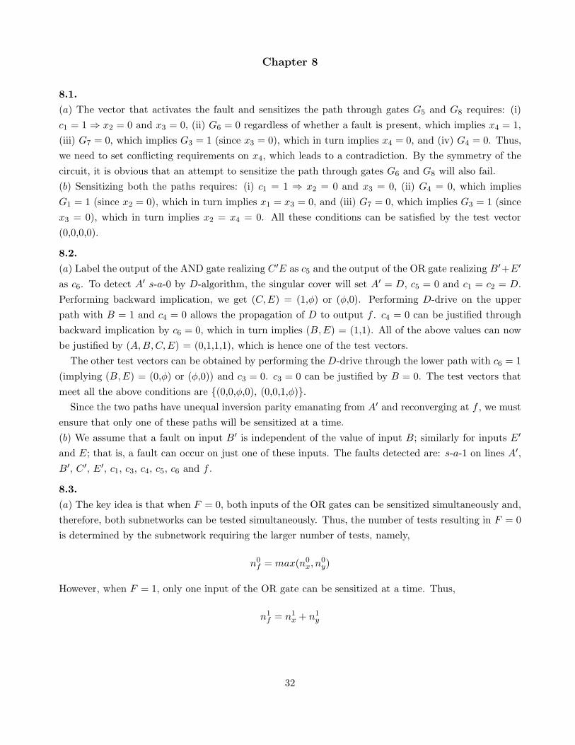
8.11. BF < c1, c2 > detected by < c1 = 0, c2 = 1 > or < c1 = 1, c2 = 0 >.
(i) < c1 = 0, c2 = 1 >: c1 = 0 for x1(x2 + x′
3 + x′
4) and c2 = 1 for x′
5. Thus, gate G1 in the gate-level
model below realizes x1(x2 + x′
3 + x′
4)x′
5.
(ii) < c1 = 1, c2 = 0 >: c1 = 1 for x′
1 and c2 = 0 for x5x′
6. Thus, gate G2 realizes x′
1x5x′
6.
G1
x1
x1
x4
x5
x5
G2
G
x6
x3
x2
f
Target fault: f SA0.
Tests
x1 x2 x3 x4 x5 x6
1 1 φ φ 0 φ1 φ 0 φ 0 φ1 φ φ 0 0 φ0 φ φ φ 1 0
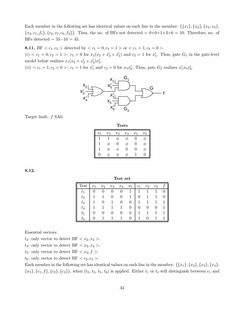
8.12.
Test set
Test x1 x2 x3 x4 x5 c1 c2 c3 f
t1 0 0 0 0 1 1 1 1 0t2 1 1 0 0 1 0 1 1 0t3 1 0 1 0 0 1 1 1 1t4 1 1 1 1 0 0 0 0 1t5 0 0 0 0 0 1 1 1 1t6 0 1 1 1 0 1 0 1 1
Essential vectors:
t2: only vector to detect BF < x2, x4 >.
t3: only vector to detect BF < x3, x4 >.
t5: only vector to detect BF < x3, f >.
t6: only vector to detect BF < c2, c3 >.
Each member in the following set has identical values on each line in the member: {{x1}, {x2}, {x3}, {x4},{x5}, {c1, f}, {c2}, {c3}}, when (t2, t3, t5, t6) is applied. Either t1 or t4 will distinguish between c1 and
34
f . Therefore, there are two minimum test sets: {t1, t2, t3, t5, t6} or {t2, t3, t4, t5, t6}.
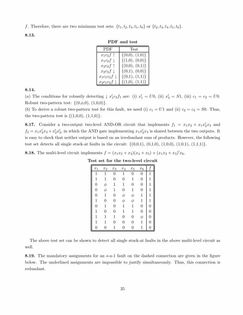
8.13.
PDF and test
PDF Test
x1c2f ↑ {(0,0), (1,0)}x1c2f ↓ {(1,0), (0,0)}x2c3f ↑ {(0,0), (0,1)}x2c3f ↓ {(0,1), (0,0)}
x1c1c3f ↓ {(0,1), (1,1)}x2c1c2f ↓ {(1,0), (1,1)}
8.14.
(a) The conditions for robustly detecting ↓ x′
1c3f1 are: (i) x′
1 = U0, (ii) x′
3 = S1, (iii) c1 = c2 = U0.
Robust two-pattern test: {(0,φ,0), (1,0,0)}.(b) To derive a robust two-pattern test for this fault, we need (i) c1 = U1 and (ii) c2 = c3 = S0. Thus,
the two-pattern test is {(1,0,0), (1,1,0)}.
8.17. Consider a two-output two-level AND-OR circuit that implements f1 = x1x2 + x1x′
2x3 and
f2 = x1x′
2x3 +x′
2x′
3, in which the AND gate implementing x1x′
2x3 is shared between the two outputs. It
is easy to check that neither output is based on an irredundant sum of products. However, the following
test set detects all single stuck-at faults in the circuit: {(0,0,1), (0,1,0), (1,0,0), (1,0,1), (1,1,1)}.
8.18. The multi-level circuit implements f = (x1x2 + x3)(x4 + x5) + (x1x2 + x3)′x6.
Test set for the two-level circuit
x1 x2 x3 x4 x5 x6 f
1 1 0 1 0 0 11 1 0 0 1 0 10 φ 1 1 0 0 10 φ 1 0 1 0 10 1 0 φ φ 1 11 0 0 φ φ 1 10 1 0 1 1 0 01 0 0 1 1 0 01 1 1 0 0 φ 01 1 0 0 0 1 00 0 1 0 0 1 0
The above test set can be shown to detect all single stuck-at faults in the above multi-level circuit as
well.
8.19. The mandatory assignments for an s-a-1 fault on the dashed connection are given in the figure
below. The underlined assignments are impossible to justify simultaneously. Thus, this connection is
redundant.
35

AND
G5=0 G8=1 x6=1
G2=0G1=0
AND OR
G7=1G4=1
ANDAND
x3=1 G1=1 G3=1G6=1
x2=1x1=1x4=1
X
AND
In the presence of the above redundant connection, c1 s-a-1 and c2 s-a-1 become redundant at f2
(note that c1 s-a-1 is not redundant at f1). Redundancy of c1 s-a-1 at f2 can be observed from the
mandatory assignments below (the underlined assignments are impossible to satisfy simultaneously).
AND
G7=0 G5=1 x6=1G1=0
G2=1
AND
x3=1
x5=1x3=0
Similarly, c2 s-a-1 can be shown to be redundant. Even after removing the impact of c1 s-a-1 at f2
(basically, replacing G4 by x3), c2 s-a-1 remains redundant. Thus, after removing these two faults, we
get the following circuit.
x1
x2
f1
x4
x5
f2
x3
x2x6
x3
8.20. Consider the redundant s-a-0 fault at c1 in the following figure. Its region is only gate G1. Next,
consider the redundant s-a-1 fault at c2. Its region is the whole circuit.
36
x1c1
x1
x2
x2 c2
G1
G2
8.21. f = x1x2 + x1x2x3 + x1x′
2 = y1 + y2 + y3.
DOBS2 = [(y1 + y3) ⊕ 1]′ = (y1 + y3)
Simplifying y2 with don’t cares y1 + y3, we get y2 = 0 since don’t care y1 = x1x2 can be made 0.
Therefore, f = y1 + y3 and DOBS1 = y3. Simplifying y1 with don’t cares in y3 = x1x′
2, we get y1 = x1
by making don’t care y3 = 1. Therefore, f = y1 + y3 where y1 = x1, y3 = x1x′
2. DOBS3 = y1.
Simplifying y3 with don’t care y1, we get y3 = 0. Therefore, f = y1 = x1.
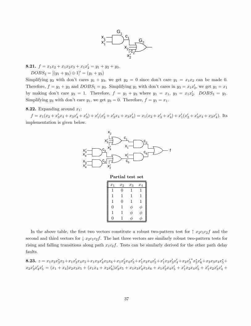
8.22. Expanding around x1:
f = x1(x2 + x′
3x4 + x3x′
4 + x′
3) + x′
1(x′
2 + x′
3x4 + x3x′
4) = x1(x2 + x′
3 + x′
4) + x′
1(x′
2 + x′
3x4 + x3x′
4). Its
implementation is given below.
x1x3 fx4
x4
x3
x2
x2
x3
c3
c4
x4
c2
c6
c1
c5
x1
Partial test set
x1 x2 x3 x4
1 0 1 11 1 1 11 0 1 10 1 φ φ1 1 φ φ0 1 φ φ
In the above table, the first two vectors constitute a robust two-pattern test for ↑ x2c1c2f and the
second and third vectors for ↓ x2c1c2f . The last three vectors are similarly robust two-pattern tests for
rising and falling transitions along path x1c2f . Tests can be similarly derived for the other path delay
faults.
8.23. z = x1x2x∗
3x5+x1x′
3x4x5+x1x3x′
4x5x6+x1x′
2x4x′
5+x′
1x2x4x′
5+x′
1x2x′
3x′
4+x2x′
3∗x∗
5x′
6+x2x3x4x∗
5+
x2x′
3x′
4x′
5 = (x1 + x4)x2x3x5 + (x1x4 + x2x′
6)x′
3x5 + x1x3x′
4x5x6 + x1x′
2x4x′
5 + x′
1x2x4x′
5 + x′
1x2x′
3x′
4 +
37

x2x′
3x′
4x′
5.
8.24. Proof available in Reference [8.11].
8.25. Proof available in Reference [8.11].
8.26. The threshold gate realizes the function x1x2x3 + x2x3x4 + x1x2x4. The AND gate realizes the
function x′
1x′
3. The test vector is: (0,1,1,0).
8.27. Proof available in Reference [8.11].
38

Chapter 9
9.1.
(a)
J1 = y2 K1 = y′2 J2 = x K2 = x′ z = x′y2 + y1y′
2 + xy′1
(b)
Excitation/output tables
x = 0 x = 1 zy1y2 J1K1 J2K2 J1K1 J2K2 x = 0 x = 1
00 01 01 01 10 0 101 10 01 10 10 1 111 10 01 10 10 1 010 01 01 01 10 1 1
(c)
State table
NS, zPS x = 0 x = 1
00 → A A, 0 B, 101 → B D, 1 C, 111 → C D, 1 C, 010 → D A, 1 B, 1
A
D C
B
0/0
1/0
0/1
0/1
1/1
0/11/1
1/1
State diagram.
From the state diagram, it is obvious that the machine produces a zero output value if and only if
the last three input values were identical (under the assumption that we ignore the first two output
symbols).
39
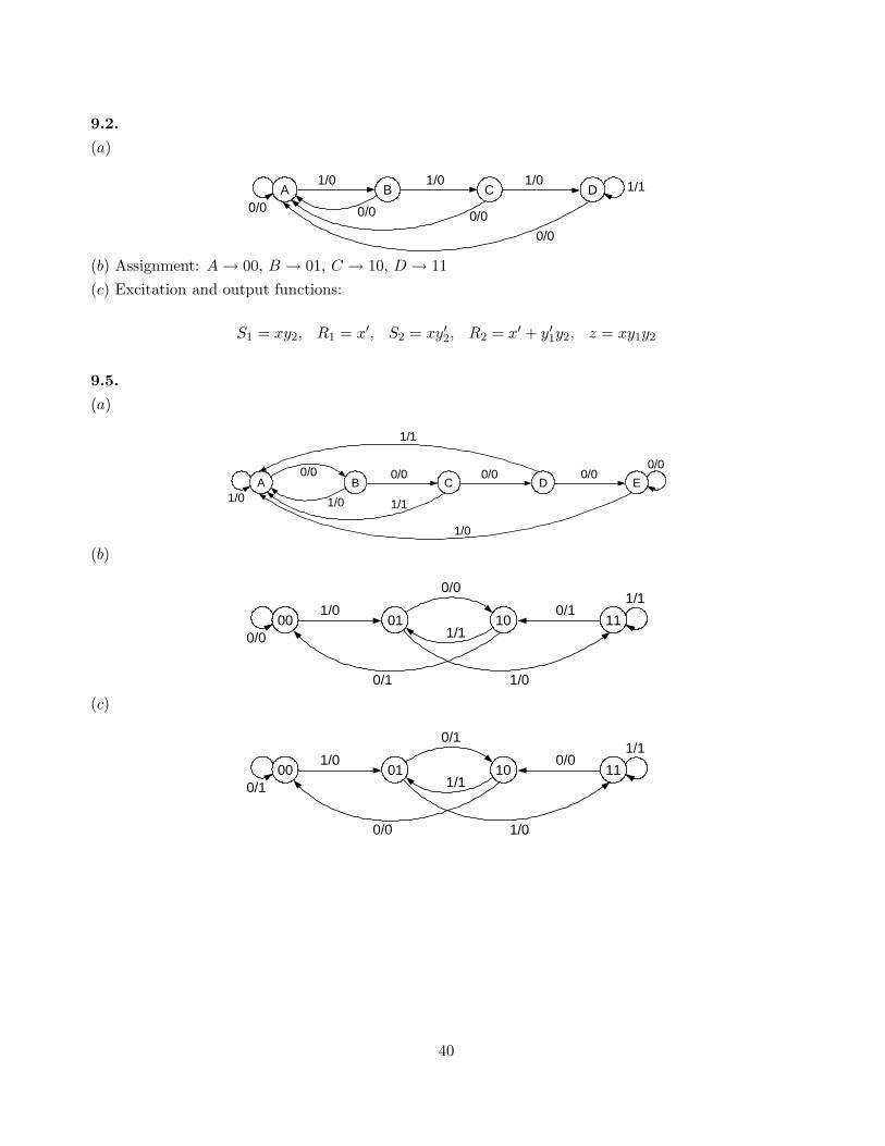
9.2.
(a)
A B C D0/0
0/0
1/11/0
0/00/0
1/0 1/0
(b) Assignment: A → 00, B → 01, C → 10, D → 11
(c) Excitation and output functions:
S1 = xy2, R1 = x′, S2 = xy′2, R2 = x′ + y′1y2, z = xy1y2
9.5.
(a)
A B C D
0/00/0
1/1
1/0
0/00/00/0
1/0E
1/0
1/1
(b)
00 01 10 110/1
1/11/0
0/1
0/0
0/0
1/0
1/1
(c)
00 01 10 110/0
1/11/0
0/0
0/1
0/1
1/0
1/1
40
(d)
001
010
011
0/0
1/1
1/0
1/1
000 1/01/0
0/1 110
111
0/1
101
100
0/0
0/0
1/0
0/0
1/0
1/1
0/0
0/1
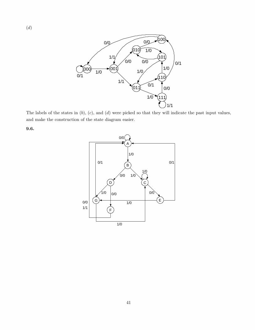
The labels of the states in (b), (c), and (d) were picked so that they will indicate the past input values,
and make the construction of the state diagram easier.
9.6.
B
D C
F
0/0
0/0 1/0
1/0
0/01/0
1/1
EG
A
0/0
1/0
1/0
1/0
0/0
0/1 0/1
41
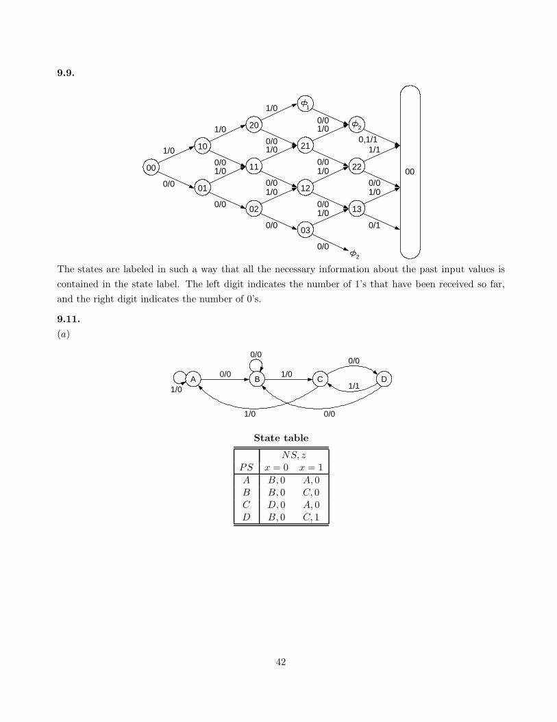
9.9.
00
0/0
1/0
2
22
0/0
1/1
03
0/0
1/0
12
0/0
1/0
21
0/0
1/00/0
0,1/1
02
0/0
1/0
11
0/0
1/0
20
0/0
1/0
01
0/0
1/0
10
0/0
1/0
13
0/1
1/0
00
2
1
The states are labeled in such a way that all the necessary information about the past input values is
contained in the state label. The left digit indicates the number of 1’s that have been received so far,
and the right digit indicates the number of 0’s.
9.11.
(a)
A B C D
0/0
1/0
1/0
1/0
0/0
0/0
0/0
1/1
State table
NS, zPS x = 0 x = 1
A B, 0 A, 0B B, 0 C, 0C D, 0 A, 0D B, 0 C, 1
42

(b)
Transition table
Y1Y2 zy1y2 x = 0 x = 1 x = 0 x = 1
00 01 00 0 001 01 11 0 011 10 00 0 010 01 11 0 1
(c)
yS
R y+
U
V
(S = U,R = U ⊕ V ) ⇒ (U = S, V = R ⊕ S)
Thus, the excitation table of one flip-flop is:
State table
y → Y S R U V
0 → 0 0 φ 0 φ0 → 1 1 0 1 11 → 0 0 1 0 11 → 1 φ 0 0 0
φ 0 1 1
Note that in the 1 → 1 case, we can choose U and V to be either 0’s or 1’s, but they must be identical.
Excitation table
x = 0 x = 1 zy1y2 U1V1 U2V2 U1V1 U2V2 x = 0 x = 1
00 0φ 11 0φ 0φ 0 001 0φ 11 11 11 0 011 11 01 01 01 0 010 01 11 11 11 0 1
From the above table, we find one possible set of equations:
U1 = x′y1y2 + xy′1y2 + xy1y′
2
V1 = 1
43

U2 = y′1y2 + y1y′
2 + x′y′1
V2 = 1
9.12.
(a) The excitation requirements for a single memory element can be summarized as follows:
Present Next Required
state state excitation
0 0 00 1 11 0 φ1 1 impossible
The state assignment must be chosen such that neither memory element will ever be required to go from
state 1 to state 1. There are two such assignments:
Assignment α Assignment β
A → 11 A → 11B → 00 B → 00C → 10 C → 01D → 01 D → 10
Assignment α yields the following excitation table and logic equations.
Y1Y2, zy1y2 x = 0 x = 1
11 φφ, 0 φφ, 000 10, 0 11, 110 φ0, 0 φ1, 001 1φ, 0 0φ, 1
Y1 = x′ + y′2
Y2 = x
z = xy′1
Assignment β yields the same equations except for an interchange of subscripts 1 and 2.
(b) The constraint that no memory element can make a transition from state 1 to state 1 means that not
all state tables can be realized with a number of memory elements equal to the logarithm of the number
of states. An n-state table can always be realized by using an n-variable assignment in which each state
is represented by a “one-out-of-n” coding. Such assignments are not necessarily the best that can be
achieved and, in general, it may be very difficult to find an assignment using the minimum number of
state variables.
9.13. The reduced state table in standard form is as follows.
44

NS, zPS x = 0 x = 1
A A, 0 B, 1B A, 1 C, 1C A, 1 D, 1D E, 0 D, 1E F, 0 D, 0F A, 0 D, 0
9.15.
A B
1/0
1/10/0
0/1
Machine M
(b) An output of 0 from machine N identifies the final state as B, while an output of 1 identifies the
final state as A. Once the state of N is known, it is straightforward to determine the input to N and
the state to which N goes by observing its output. Consequently, except for the first bit, each of the
subsequent bits can be decoded.
9.16. A simple strategy can be employed here whereby the head moves back and forth across the block
comparing the end symbols and, whenever they are identical, replacing them with 2’s and 3’s (for 0’s
and 1’s, respectively). At the end of the computation, the original symbols are restored.
NS, write, shiftPS # 0 1 2 3
A B,#, R A, 0, R A, 1, R A, 0, R A, 1, RB C, 2, R D, 3, R I, 2, L I, 3, LC E,#, L C, 0, R C, 1, R E, 2, L E, 3, LD F,#, L D, 0, R D, 1, R F, 2, L F, 3, LE G, 2, L H, 1, L I, 2, LF H, 0, L G, 3, L I, 3, LG G, 0, L G, 1, L B, 2, R B, 3, RH A,#, R H, 0, L H, 1, L H, 2, L H, 3, LI J,#, R I, 0, L I, 1, L I, 2, L I, 3, LI Halt J, 0, R J, 1, R J, 0, R J, 1, R
Halt Halt Halt Halt
state A. Starting state. The machine restores the original symbols of the present block and moves to
test the next block.
state B. (columns 0,1): The head checks the leftmost original symbol of the block.
(columns 2,3): A palindrome has been detected.
45

states C and D. (#,0,1,2,3): The head searches for the rightmost original symbol of the block. State
C is for the case that the leftmost symbol is a 0, and D for the case that it is a 1.
states E and F. (0,1): The head checks the rightmost symbol and compares it with the leftmost
symbol. (E is for 0 and F is for 1.)
(2,3): At this point, the machine knows that the current symbol is the middle of an odd-length
palindrome.
state G. The symbols that were checked so far can be members of a palindrome.
(0,1,2,3): The head searches for the leftmost original symbol of the block.
state H. At this point, the machine knows that the block is not a palindrome.
(0,1,2,3): The head goes to the beginning of the block, so that it will be ready to restore the original
symbols (as indicated in state A).
state I. The machine now knows that the block is a palindrome. Therefore, the head goes to the
beginning of the block, so that it will be ready to restore the original symbols (as indicated in state J).
states J and Halt: The original symbols are restored and the machine stops at the first # to the right
of the block.
9.18.
0/0 0/11/0 0/1
1/0
0/0 1/1
C
DI
A
B
E1/1
0/01/0
1/0
0/0
State I is an initial state and it appears only in the first cell. It is not a necessary state for all other
cells. We may design the network so that the first cell that detects an error will produce output value 1
and then the output values of the next cells are unimportant. In such a case, state E is redundant and
the transitions going out from C and D with a 1 output value may be directed to any arbitrary state
φ. The reduced state and excitation tables are as follows:
NS, zi
PS xi = 0 xi = 1
A A, 0 C, 0B D, 0 B, 0C φ, 1 C, 0D D, 0 φ, 1
Yi1Yi2, zi
yi1yi2 xi = 0 xi = 1
00 00, 0 11, 001 10, 0 01, 011 φφ, 1 11, 010 10, 0 φφ, 1
zi = x′
iyi1yi2 + xiyi1y′
i2
46

Yi1 = x′
iyi2 + xiy′
i2 + yi1
Yi2 = xi
If state E is retained, the realization will require three state variables.
9.19.
(a)
A B C D0/1
1/0
1/0
0/0
0/0
0/0
1/1
1/0
State A corresponds to an even number of zeros, B to an odd number of zeros, C to an odd number of
ones, and D to an even number of ones.
NS, zi
PS xi = 0 xi = 1
A B, 0 C, 0B A, 0 C, 1C B, 1 D, 0D B, 0 C, 0
(b) The assignment and the corresponding equations are given next: A → 00, B → 01, C → 11, D → 10.
Yi1 = xi
Yi2 = y′i2 + xiy′
i1yi2 + x′
iyi1yi2
zi = xiy′
i1yi2 + x′
iyi1yi2
9.20.
NS, zi
PS xi = 0 xi = 1
A A, 0 B, 1B C, 0 D, 1C A, 1 B, 0D C, 1 D, 0
Yi1Yi2, zi
yi1yi2 xi = 0 xi = 1
00 00, 0 01, 101 11, 0 10, 111 00, 1 01, 010 11, 1 10, 0
Yi1 = yi1 ⊕ yi2
Yi2 = xi ⊕ yi1 ⊕ yi2
zi = xi ⊕ yi1
47
Chapter 10
10.1.
(a) Suppose the starting state is S1, then one input symbol is needed to take the machine to another
state, say S2. Since the machine is strongly connected, at most two symbols are needed to take the
machine to a third state, say S3. (This occurs if S3 can be reached from S1 and not from S2.) By the
same line of reasoning, we find that the fourth distinct state can be reached from S3 by at most three
input symbols. Thus, for an n-state machine, the total number of symbols is at most∑n−1
i=1 i = n2 (n−1).
This is not a least upper bound. It is fairly easy to prove, for example, that the least upper bound for
a three-state machine is 2 and not 3, which is given by the above bound. In other words, there exists
no three-state strongly connected machine that needs more than two input symbols to go through each
of its states once.
(b)
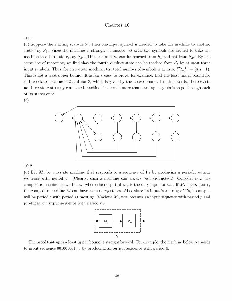
10.2.
(a) Let Mp be a p-state machine that responds to a sequence of 1’s by producing a periodic output
sequence with period p. (Clearly, such a machine can always be constructed.) Consider now the
composite machine shown below, where the output of Mp is the only input to Mn. If Mn has n states,
the composite machine M can have at most np states. Also, since its input is a string of 1’s, its output
will be periodic with period at most np. Machine Mn now receives an input sequence with period p and
produces an output sequence with period np.
Mp
M
Mn
The proof that np is a least upper bound is straightforward. For example, the machine below responds
to input sequence 001001001. . . by producing an output sequence with period 6.
48
A B
1/1
0/01/0
0/0
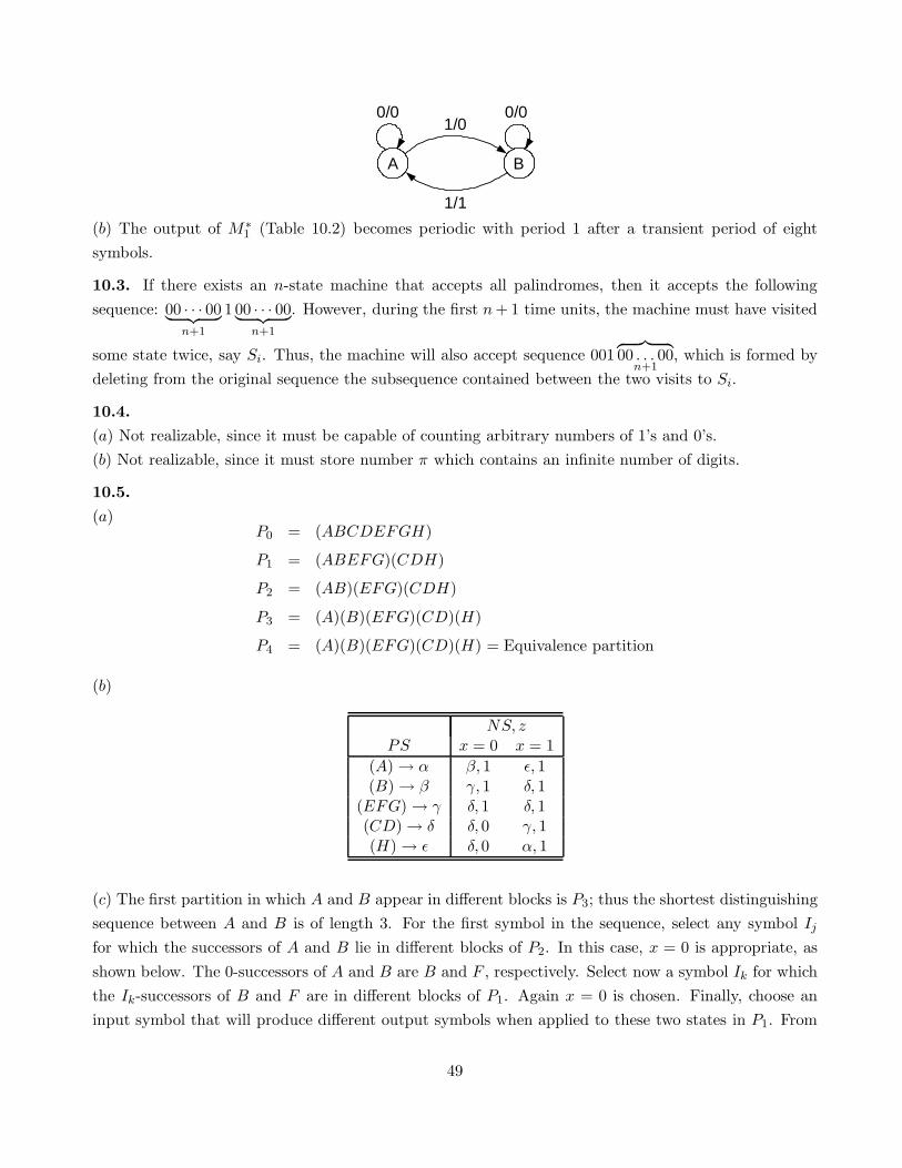
(b) The output of M∗
1 (Table 10.2) becomes periodic with period 1 after a transient period of eight
symbols.
10.3. If there exists an n-state machine that accepts all palindromes, then it accepts the following
sequence: 00 · · · 00︸ ︷︷ ︸
n+1
1 00 · · · 00︸ ︷︷ ︸
n+1
. However, during the first n + 1 time units, the machine must have visited
some state twice, say Si. Thus, the machine will also accept sequence 001︷ ︸︸ ︷
00 . . . 00n+1
, which is formed by
deleting from the original sequence the subsequence contained between the two visits to Si.
10.4.
(a) Not realizable, since it must be capable of counting arbitrary numbers of 1’s and 0’s.
(b) Not realizable, since it must store number π which contains an infinite number of digits.
10.5.
(a)P0 = (ABCDEFGH)
P1 = (ABEFG)(CDH)
P2 = (AB)(EFG)(CDH)
P3 = (A)(B)(EFG)(CD)(H)
P4 = (A)(B)(EFG)(CD)(H) = Equivalence partition
(b)
NS, zPS x = 0 x = 1
(A) → α β, 1 ǫ, 1(B) → β γ, 1 δ, 1
(EFG) → γ δ, 1 δ, 1(CD) → δ δ, 0 γ, 1(H) → ǫ δ, 0 α, 1
(c) The first partition in which A and B appear in different blocks is P3; thus the shortest distinguishing
sequence between A and B is of length 3. For the first symbol in the sequence, select any symbol Ij
for which the successors of A and B lie in different blocks of P2. In this case, x = 0 is appropriate, as
shown below. The 0-successors of A and B are B and F , respectively. Select now a symbol Ik for which
the Ik-successors of B and F are in different blocks of P1. Again x = 0 is chosen. Finally, choose an
input symbol that will produce different output symbols when applied to these two states in P1. From
49
the illustration below, it is evident that 000 is the minimum-length sequence that distinguishes state A
from state B.
P0 = (ABCDEFGH)
x = 0
P3 = (A)(B)(EFG)(CD)(H)
P2 = (AB)(EFG)(CDH)
P1 = (ABEFG)(CDH)z = 0
z = 1
x = 0
x = 0
z = 1z = 1
z = 1
z = 1
10.6.
(a) P = (A)(BE)(C)(D)
(b) P = (AB)(C)(D)(E)(FG)
(c) P = (A)(B)(CD)(EFG)(H)
10.7. From column Ii, we find
(A,B)Ii
(A,C) (A,D) (A,H)
Ii
IiIiIi
Thus, if A is equivalent to any one of the other states, it must be equivalent to all of them. From
column Ij , we conclude that if state B is equivalent to any other state, then A must also be equivalent
to some state, which means that all the states are equivalent. Using the same argument, we can show
that no two states are equivalent unless all the states are equivalent.
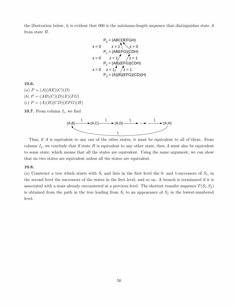
10.8.
(a) Construct a tree which starts with Si and lists in the first level the 0- and 1-successors of Si, in
the second level the successors of the states in the first level, and so on. A branch is terminated if it is
associated with a state already encountered at a previous level. The shortest transfer sequence T (Si, Sj)
is obtained from the path in the tree leading from Si to an appearance of Sj in the lowest-numbered
level.
50

(b)
0
x=0
ALevel
0
x=1
BA
C D
F E
1
1
3
2
1
0
G B
1
0
E D
1
4
0
G A
1 0
G A
1
There are three minimal transfer sequences T (A,G), namely 1110, 1100, and 1000.
10.9.
(a) Construct a tree which starts with the pair (SiSj). Then, for every input symbol, the two successor
states will be listed separately if they are associated with different output symbols, and will form a new
pair if the output symbols are the same. A branch of the tree is terminated if it is associated with a
pair of states already encountered at a previous level, or if it is associated with a pair of identical states,
i.e., (SkSk). A sequence that distinguishes Si from Sj is one that can be described by a path in the tree
that leads from (SiSj) to any two separately listed states, e.g., (Sp)(Sq).
(b)
0
x=0
(AG)
0
x=1
(BF)(AC)
(CG) (BD)
(CF) (DE)
1
1
(BE)
0
(CE) (DF)
1
0
(EG) (AD)
1 0 1 0 1 0 1
0
(AE) (BD)
1
0 1
0 1
(FG) (EG) (B)(D) (FG) (A)(E)(B)(D)
(AB)(AG)
(AC)
There are five sequences of four symbols each that can distinguish A from G: 1111, 1101, 0111, 0101,
51

0011.
10.10.
(a)
P0 = (ABCDEFGH)
P1 = (AGH)(BCDEF )
P2 = (AH)(G)(BDF )(CE)
P3 = (AH)(G)(BDF )(CE)
Thus, A is equivalent to H.
(b) From P3, we conclude that for each state of M1, there exists an equivalent state in M2 that is, H is
equivalent to A, F is equivalent to B and D, and E is equivalent to C.
(c) M1 and M2 are equivalent if their initial states are either A and H, or B and F , or D and F , or C
and E.
10.13.
X: 0 0 0 0 1 0 1 0 0 0 1 0
A
Z: 1 0 1 0 0 1 1 0 0 0 0 1
S: ACCCCBAABAB
Observing the input and output sequences, we note that during the experiment the machine responded
to 00 by producing 10, 01, and 00. This indicates that the machine has three distinct states, which we
shall denote A, B, and C, respectively. (These states are marked by one underline). At this point, we
can determine the transitions from A, B, and C under input symbol 0, as indicated by the entries with
double underlines. In addition, we conclude that A is the only state that responds by producing a 1
output symbol to a 0 input symbol. Thus, we can add two more entries (A with three underlines) to the
state-transition row above. The machine in question indeed has three states and its state transitions
and output symbols are given by the state table below:
NS, zPS x = 0 x = 1
A B, 1 A, 0B A, 0 C, 1C C, 0 A, 0
10.16. Find the direct sum M of M1 and M2. M has n1 + n2 states and we are faced with the problem
of establishing a bound for an experiment that distinguishes between Si and Sj in M . From Theorem
52
10.2, the required bound becomes evident.
10.17. Modify the direct sum concept (see Problem 10.10) to cover incompletely specified machines.
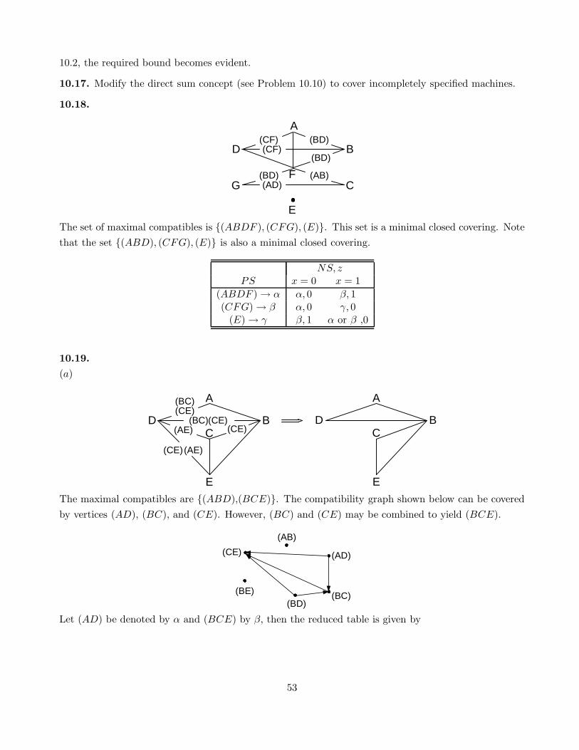
10.18.
A
B
F
(CF)D(BD)(CF)
(BD)
(AD)(AB)(BD)
CG
E
The set of maximal compatibles is {(ABDF ), (CFG), (E)}. This set is a minimal closed covering. Note
that the set {(ABD), (CFG), (E)} is also a minimal closed covering.
NS, zPS x = 0 x = 1
(ABDF ) → α α, 0 β, 1(CFG) → β α, 0 γ, 0
(E) → γ β, 1 α or β ,0
10.19.
(a)
A
B
E
D (CE)(CE)
(CE)(AE) C(BC)
(BC)
(CE) (AE)
A
B
E
DC
The maximal compatibles are {(ABD),(BCE)}. The compatibility graph shown below can be covered
by vertices (AD), (BC), and (CE). However, (BC) and (CE) may be combined to yield (BCE).
(BC)
(AB)
(BE)
(CE)
(BD)
(AD)
Let (AD) be denoted by α and (BCE) by β, then the reduced table is given by
53
NS, zPS I1 I2 I3
α β, 0 β, 1 β,−β β, 0 β, 0 α,−
(b) The minimal set of compatibles is {(AB), (AE), (CF ), (DF )}.
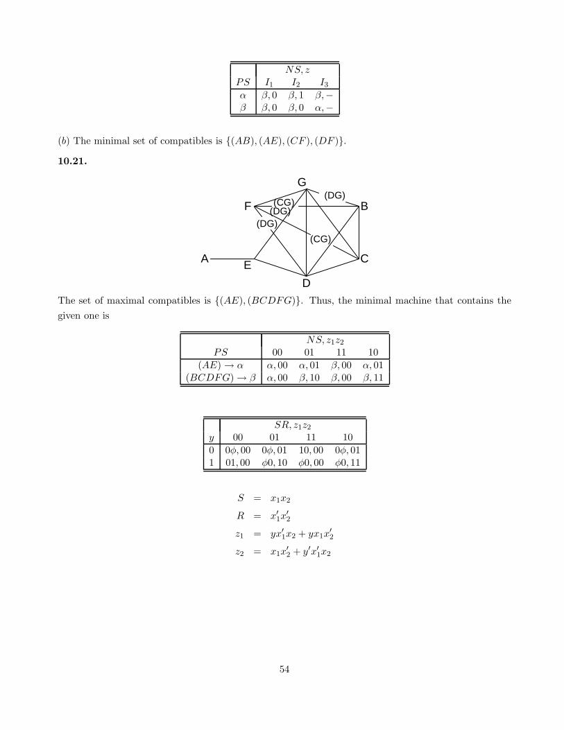
10.21.
G
B
C
D
E
(CG)
(CG)
F
A
(DG)
(DG)(DG)
The set of maximal compatibles is {(AE), (BCDFG)}. Thus, the minimal machine that contains the
given one is
NS, z1z2
PS 00 01 11 10
(AE) → α α, 00 α, 01 β, 00 α, 01(BCDFG) → β α, 00 β, 10 β, 00 β, 11
SR, z1z2
y 00 01 11 10
0 0φ, 00 0φ, 01 10, 00 0φ, 011 01, 00 φ0, 10 φ0, 00 φ0, 11
S = x1x2
R = x′
1x′
2
z1 = yx′
1x2 + yx1x′
2
z2 = x1x′
2 + y′x′
1x2
54
Chapter 11
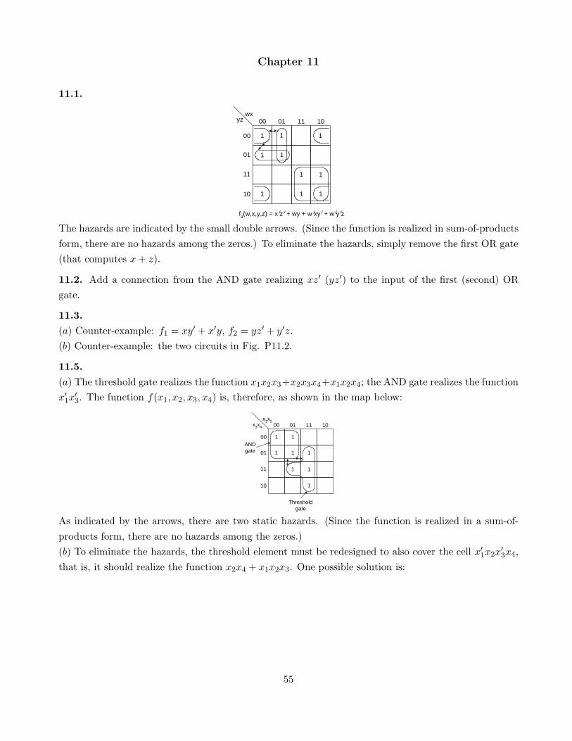
11.1.
11
1
1
1
1
1
1
00 01 11 10
fa(w,x,y,z) = x z + wy + w xy + w y z
00
01
11
10
wxyz
1
1
The hazards are indicated by the small double arrows. (Since the function is realized in sum-of-products
form, there are no hazards among the zeros.) To eliminate the hazards, simply remove the first OR gate
(that computes x + z).
11.2. Add a connection from the AND gate realizing xz′ (yz′) to the input of the first (second) OR
gate.
11.3.
(a) Counter-example: f1 = xy′ + x′y, f2 = yz′ + y′z.
(b) Counter-example: the two circuits in Fig. P11.2.
11.5.
(a) The threshold gate realizes the function x1x2x3+x2x3x4+x1x2x4; the AND gate realizes the function
x′
1x′
3. The function f(x1, x2, x3, x4) is, therefore, as shown in the map below:
1
1
1
1
1
1
00 01 11 10
00
01
11
10
x1x2
ANDgate
x3x4
1
1
Thresholdgate
As indicated by the arrows, there are two static hazards. (Since the function is realized in a sum-of-
products form, there are no hazards among the zeros.)
(b) To eliminate the hazards, the threshold element must be redesigned to also cover the cell x′
1x2x′
3x4,
that is, it should realize the function x2x4 + x1x2x3. One possible solution is:
55

x2x4 + x1x2x3x3
x2
x1
x4
13
2
921
11.7.
(a) The four bidirectional arrow in the K-map below show the eight MIC transitions that have a function
hazard.
1
1
1 1
xyz
0
1
00 01 11 10
1
1
00
(b) The required cubes {xy, yz} and privileged cube {y} are shown below.
1
1
1 1
xyz
0
1
00 01 11 10
1
1
00
(c) The required cubes {x, z} are shown below.
1
1
1 1
xyz
0
1
00 01 11 10
1
1
00
11.8.
(a) The required cubes, privileged cubes and dhf-prime implicants are shown below.
1
1
1
1
1
0
1
00 01 11 10
00
01
11
10
wxyz
01
0
1
1
1
0
1
1
(b) Hazard-free sum of products: w′x′y′ + y′z + wy′ + w′y + wxz.
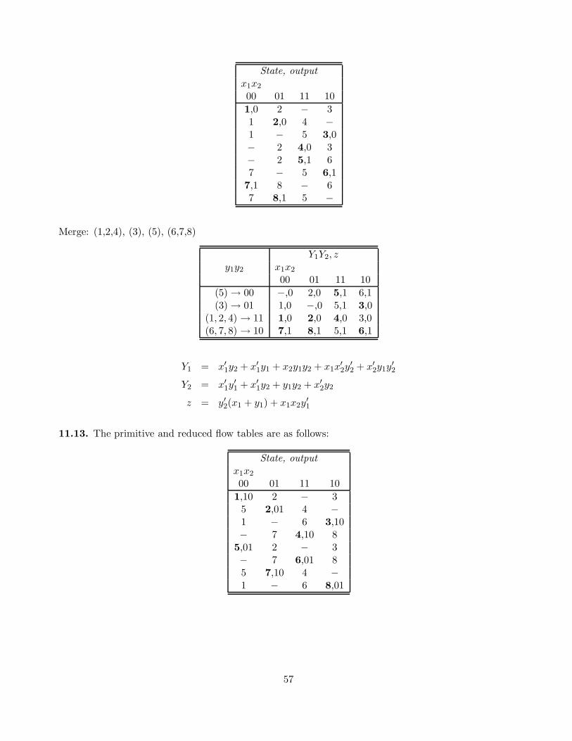
11.12. The reduced table shown below is derived from the following primitive table and the correspond-
ing merger graph.
56
State, output
x1x2
00 01 11 10
1,0 2 − 31 2,0 4 −1 − 5 3,0− 2 4,0 3− 2 5,1 67 − 5 6,1
7,1 8 − 67 8,1 5 −
Merge: (1,2,4), (3), (5), (6,7,8)
Y1Y2, zy1y2 x1x2
00 01 11 10
(5) → 00 −,0 2,0 5,1 6,1(3) → 01 1,0 −,0 5,1 3,0
(1, 2, 4) → 11 1,0 2,0 4,0 3,0(6, 7, 8) → 10 7,1 8,1 5,1 6,1
Y1 = x′
1y2 + x′
1y1 + x2y1y2 + x1x′
2y′
2 + x′
2y1y′
2
Y2 = x′
1y′
1 + x′
1y2 + y1y2 + x′
2y2
z = y′2(x1 + y1) + x1x2y′
1
11.13. The primitive and reduced flow tables are as follows:
State, output
x1x2
00 01 11 10
1,10 2 − 35 2,01 4 −1 − 6 3,10− 7 4,10 8
5,01 2 − 3− 7 6,01 85 7,10 4 −1 − 6 8,01
57

6
8 1
3
2
5
7
4
Y1Y2, z1z2
y1y2 x1x2
00 01 11 10
(1, 3) → 00 1,10 2 6 3(2, 5) → 01 5,01 2,01 4 3(4, 7) → 11 5 7,10 4,10 8(6, 8) → 10 1 7 6,01 8,01
Y1 = x1x2 + x2y1 + x1y1
= [(x1x2)′(x2y1)
′(x1y1)′]′
Y2 = x′
1x2 + x2y2 + x′
1y2
= [(x′
1x2)′(x2y2)
′(x′
1y2)′]′
If we regard the unspecified outputs as don’t-care combinations, we obtain
z1 = y′1y′
2 + y1y2 = [(y′1y′
2)′(y1y2)
′]′
z2 = y′1y2 + y1y′
2 = [(y′1y2)′(y1y
′
2)′]′
11.15.
x1
Street
Railroad
lights
x2
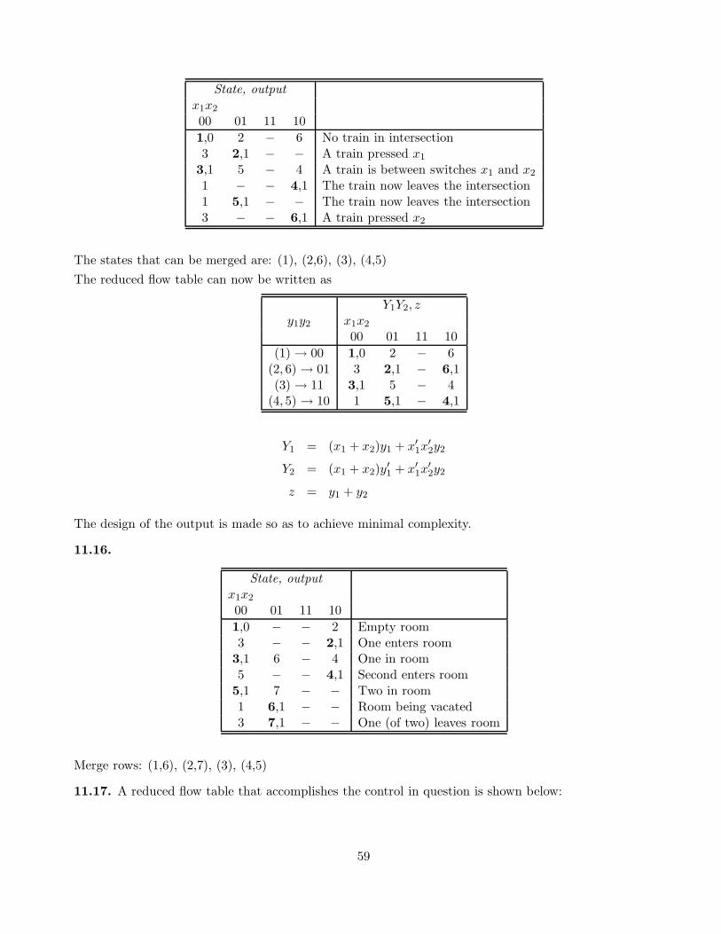
(a) Switches x1 and x2 are each placed 1500 feet from the intersection. The primitive flow table that
describes the light control is as follows:
58
State, output
x1x2
00 01 11 10
1,0 2 − 6 No train in intersection3 2,1 − − A train pressed x1
3,1 5 − 4 A train is between switches x1 and x2
1 − − 4,1 The train now leaves the intersection1 5,1 − − The train now leaves the intersection3 − − 6,1 A train pressed x2
The states that can be merged are: (1), (2,6), (3), (4,5)
The reduced flow table can now be written as
Y1Y2, zy1y2 x1x2
00 01 11 10
(1) → 00 1,0 2 − 6(2, 6) → 01 3 2,1 − 6,1(3) → 11 3,1 5 − 4
(4, 5) → 10 1 5,1 − 4,1
Y1 = (x1 + x2)y1 + x′
1x′
2y2
Y2 = (x1 + x2)y′
1 + x′
1x′
2y2
z = y1 + y2
The design of the output is made so as to achieve minimal complexity.
11.16.
State, output
x1x2
00 01 11 10
1,0 − − 2 Empty room3 − − 2,1 One enters room
3,1 6 − 4 One in room5 − − 4,1 Second enters room
5,1 7 − − Two in room1 6,1 − − Room being vacated3 7,1 − − One (of two) leaves room
Merge rows: (1,6), (2,7), (3), (4,5)
11.17. A reduced flow table that accomplishes the control in question is shown below:
59

State, output
P1P2
00 01 11 10
A,1 D C A,1B,0 D C B,0B C,0 C,0 BA D,0 D,0 A
11.19.
(a) Whenever the inputs assume the values x1 = x2 = 1, the circuit output becomes 1 (or remains 1 if it
was already 1). Whenever the inputs assume the values x1 = 1, x2 = 0, the output becomes (or remains)
0. Whenever the inputs assume any other combination of values, the output retains its previous value.
(b) The flow table can be derived by breaking the feedback loop as shown below:
x2
y
x1
Yx2z
The excitation and output equations are then
Y = x1x2 + (x′
1 + x2)y
z = y
(c) The same function for Y can be achieved by eliminating the x2y term. This, however, creates a
static hazard in Y when y = 1, x2 = 1 and x1 changes between 0 and 1. Hence, proper operation would
require the simultaneous change of two variables. A simple solution is to place an inertial or smoothing
delay between Y and y in the figure shown above.
11.20.
Y1Y2Y3
y1y2y3 x1x2
00 01 11 10
a → 000 000 001 000 001a → 001 001 101 001 111a → 011 011 001 011 111b → 010 {001,011} 010 110 010b → 100 000 100 101 100b → 101 101 101 101 111c → 111 111 110 011 111d → 110 000 110 100 110
60

The assignment in column 00 row 010 is made so as to allow minimum transition time to states c and
d. In column 00, row 110 and column 10, row 001, we have noncritical races.
61

Chapter 12
12.1. Since the machine has n states, k = ⌈log2 n⌉ state variables are needed for an assignment. The
problem is to find the number of distinct ways of assigning n states to 2k codes. There are 2k ways to
assign the first state, 2k − 1 ways to assign the second state, etc., and 2k − n + 1 ways to assign the nth
state. Thus, there are
2k · (2k − 1) · . . . · (2k − n + 1) =2k!
(2k − n)!
ways of assigning the n states.
There are k! ways to permute (or rename) the state variables. In addition, each state variable can be
complemented, and hence there are 2k ways of renaming the variables through complementation. Thus,
the number of distinct state assignments is
2k!
(2k − n)!· 1
k!2k=
(2k − 1)!
(2k − n)!k!
12.2.
Assignment α:
Y1 = x′y′1y′
2y3 + x′y2y′
3 + xy2y3 = f1(x, y1, y2, y3)
Y2 = y′1y′
2y′
3 + xy′2 + y1y3 = f2(x, y1, y2, y3)
Y3 = x′y′1y′
2 + x′y2y3 + xy2y′
3 + xy1 = f3(x, y1, y2, y3)
z = xy′1y′
2y3 + x′y2y3 + x′y1 + y1y′
3 = f0(x, y1, y2, y3)
Assignment β:
Y1 = xy1 + x′y′1 = f1(x, y1)
Y2 = x′y3 = f2(x, y3)
Y3 = y′2y′
3 = f3(y2, y3)
z = x′y′1 + xy3 = f0(x, y1, y3)
12.3. No, since π1 + π2 is not included in the set of the given closed partitions.
12.5. Suppose π is a closed partition. Define a new partition
π′ =∑
{πSiSj|Si and Sj are in the same block ofπ}
Since π′ is the sum of closed partitions, it is itself closed. (Note that π′ is the sum of some basic
partitions.) Furthermore, since π ≥ πSiSj, for all Si and Sj which are in the same block of π, we must
have π ≥ π′. To prove that in fact π = π′, we note that if π > π′, then π would identify some pair SiSj
which is not identified by π′, but this contradicts the above definition of π′. Thus, π′ = π.
62

Since any closed partition is the sum of some basic partitions, by forming all possible sums of the
basic partitions we obtain all possible closed partitions. Thus, the procedure for the construction of the
π-lattice, outlined in Sec. 12.3, is verified.
12.7.
(a) Let us prove first that if π is a closed and output-consistent partition, then all the states in the
same block of π are equivalent. Let A and B be two states in some block of π. Since π is closed, the
k-successors of A and B, where k = 1, 2, 3, · · ·, will also be in the same block of π. Also, since π is
output consistent, just one output symbol is associated with every block of π. Thus, A and B must be
k-equivalent for all k’s.
To prove the converse, let us show that if M is not reduced, there exists some closed partition on M
which is also output consistent. Since M is not reduced, it has a nontrivial equivalence partition Pk.
Clearly, Pk is closed and output consistent. Thus, the above assertion is proved.
(b) λo = {A,C,F ;B,D,E}The only closed partition π ≤ λo is
π = {A,F ;B,E;C;D} = {α;β; γ; δ}
The reduced machine is
NSPS x = 0 x = 1 z
α β γ 0β β α 1γ β δ 0δ β γ 1
12.8. For the machine in question:
λi = {A,B;C,D}
We can also show that the partition
π = {A,B;C,D}
is closed. However, there is no way of specifying the unspecified entries in such a way that the partition
{A,B;C,D} will be input consistent and closed. (Note that, in general, in the case of incompletely
specified machines, if π1 and π2 are closed partitions, π3 = π1 + π2 is not necessarily a closed partition.)
12.9.
(i) Find π3 = π1 · π2 = {A,F ;B,E;C,H ;D,G}. The π-lattice is given by
63

( I )
( 0 )
21
3
Assign y1 to π1, y2 to π2, and y3 to λo. Since π2 ≥ λi, y2 is input independent. The schematic diagram
is given as follows:
x
y1
z
1
y2
2y3
0
(ii)
π1 = {A,B;C,D;E,F ;G,H}π2 = {A,E;B,F ;C,G;D,H}π3 = π1 + π2 = {A,B,E, F ;C,D,G,H}λo = λi = {A,B,C,D;E,F,G,H}
Note that π1 · π2 = 0 is a parallel decomposition, but requires four state variables. However, both π1
and π2 can be decomposed to yield the same predecessor, i.e.,
π3 · τ1 = π1
π3 · τ2 = π2
τ1 = {A,B,C,D;E,F,G,H} = λo = λi
τ2 = {A,C,E,G;B,D,F,H}
Xz
3
2
=01
~
~
2
discard
1
64

Since τ1 = λo, the output can be obtained from the τ1 machine, and evidently the τ2 machine
is unnecessary. (Note that π1 ≤ λo; thus the machine can be reduced, as shown by the discarded
submachine.)
12.10.
(a)
λi = {A,B;C,D;E,F ;G,H}λo = {A,C,E,G;B,D,F,H}
The π-lattice is found to be
( I )
( 0 )
2
1
{ A,B; C,D; E,F; G,H }
= { A,B,E,F; C,D,G,H }
=
(b) π1 ≥ π2 ≥ λi, so that both π1 and π2 are autonomous clocks of periods 2 and 4, respectively. Choose
τ1, such that τ1 · π1 = π2, and the following schematic diagram results.
x
~1 1
0
2
z
12.11.
(a)
λi = {A,B,C;D,E,F }λo = {A,B,C,D,E;F}
The following closed partitions are found using the procedure in Sec. 12.3.
( I )
( 0 )
21 { A,B,C; D,E,F }= { A,E; B,F; C,D } =
(b) To find f1 independent of x, we must assign y1 to λi = π2. Since f2 and f3 are functions of x, y2,
and y3, the partitions corresponding to y2 and y3 are neither input consistent nor closed. However, the
65
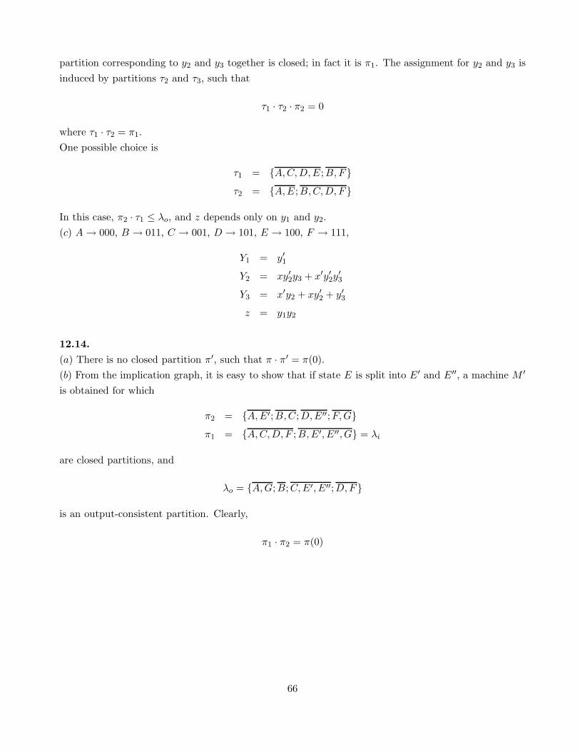
partition corresponding to y2 and y3 together is closed; in fact it is π1. The assignment for y2 and y3 is
induced by partitions τ2 and τ3, such that
τ1 · τ2 · π2 = 0
where τ1 · τ2 = π1.
One possible choice is
τ1 = {A,C,D,E ;B,F}τ2 = {A,E;B,C,D,F}
In this case, π2 · τ1 ≤ λo, and z depends only on y1 and y2.
(c) A → 000, B → 011, C → 001, D → 101, E → 100, F → 111,
Y1 = y′1
Y2 = xy′2y3 + x′y′2y′
3
Y3 = x′y2 + xy′2 + y′3
z = y1y2
12.14.
(a) There is no closed partition π′, such that π · π′ = π(0).
(b) From the implication graph, it is easy to show that if state E is split into E′ and E′′, a machine M ′
is obtained for which
π2 = {A,E′;B,C;D,E′′;F,G}π1 = {A,C,D,F ;B,E′, E′′, G} = λi
are closed partitions, and
λo = {A,G;B;C,E′, E′′;D,F}
is an output-consistent partition. Clearly,
π1 · π2 = π(0)
66

(c)
NS, zPS x = 0 x = 1
A F ,1 C,0B E′′,0 B,1C D,0 C,0D F ,1 C,1E′ G,0 B,0E′′ G,0 B,0F A,1 F ,1G E′,1 G,0
Machine M ′
Let y1 be assigned to blocks of π1, y2 to blocks of τ(y2) = {A,D,E′, E′′;B,C,F,G}, and y3 to
τ(y3) = {A,B,C,E′;D,E′′, F,G}. Clearly, τ(y2) · τ(y3) = π2.
The state tables of the component machines are:
PS NS
(A,C,D,F ) → P P(B,E′, E′′, G) → Q Q
M1
NSPS x = 0 x = 1
(A,D,E′, E′′) → R S S(B,C,F,G) → S R S
M2
NSx = 0 x = 1
PS R S R S
(A,B,C,E′) → U V V U U(D,E′′, F,G) → V V U U V
M3
(d) The state assignment induced by above partitions: A → 000, B → 110, C → 010, D → 001,
E′ → 100, E′′ → 101, F → 011, G → 111.
12.15.
(a) We shall prove that M{m[M(τ)]} = M(τ), leaving the proof that m{M [m(τ)]} = m(τ) to the
reader.
[M(τ), τ ] and {M(τ),m[M(τ)} are partition pairs, and therefore (by the definition of an m-partition)
m[M(τ)] ≤ τ . By monotonicity, M{m[M(τ)]} ≤ M(τ). On the other hand, {M(τ),m[M(τ)]} is a
partition pair, and hence, M{m[M(τ)]} ≥ M(τ). Thus, the first equality is valid.
(b) {M(τ),m[M(τ)]} is a partition pair. It is also an Mm pair, since (from part (a)), M{m[M(τ)]} =
M(τ). Similarly, {M [m(τ)],m(τ)} is an Mm pair, since m{M [m(τ)]} = m(τ).
67
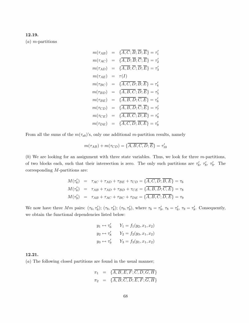
12.19.
(a) m-partitions
m(τAB) = {A,C ;B;D;E} = τ ′
1
m(τAC) = {A,D;B;C;E} = τ ′
2
m(τAD) = {A,B;C;D;E} = τ ′
3
m(τAE) = τ(I)
m(τBC) = {A,C,D;B;E} = τ ′
4
m(τBD) = {A,B,C ;D;E} = τ ′
5
m(τBE) = {A,B,D;C,E} = τ ′
6
m(τCD) = {A,B,D;C;E} = τ ′
7
m(τCE) = {A,B,C ;D,E} = τ ′
8
m(τDE) = {A,C,D;B,E} = τ ′
9
From all the sums of the m(τab)’s, only one additional m-partition results, namely
m(τAB) + m(τCD) = {A,B,C,D;E} = τ ′
10
(b) We are looking for an assignment with three state variables. Thus, we look for three m-partitions,
of two blocks each, such that their intersection is zero. The only such partitions are τ ′
6, τ ′
8, τ ′
9. The
corresponding M -partitions are:
M(τ ′
6) = τAC + τAD + τBE + τCD = {A,C,D;B,E} = τ6
M(τ ′
8) = τAB + τAD + τBD + τCE = {A,B,D;C,E} = τ8
M(τ ′
9) = τAB + τAC + τBC + τDE = {A,B,C;D,E} = τ9
We now have three Mm pairs: (τ6, τ′
6); (τ8, τ′
8); (τ9, τ′
9), where τ6 = τ ′
9, τ8 = τ ′
6, τ9 = τ ′
8. Consequently,
we obtain the functional dependencies listed below:
y1 ↔ τ ′
6 Y1 = f1(y2, x1, x2)
y2 ↔ τ ′
8 Y2 = f2(y3, x1, x2)
y3 ↔ τ ′
9 Y3 = f3(y1, x1, x2)
12.21.
(a) The following closed partitions are found in the usual manner;
π1 = {A,B,E, F ;C,D,G,H}π2 = {A,B;C,D;E,F ;G,H}
68

where π1 > π2. The maximal autonomous clock is generated by λi = {A,B;C,D;E,F ;G,H} = π2. Its
period is 4 and its state diagram is given by
AB
EF
CD GH
(b)
C1
x
C3C2 f0 z
M1 ↔ π1
M2 ↔ τ2 = {A,B,C,D;E,F,G,H},where π1 · τ2 = π2.
M3 ↔ τ3 = {A,C,E,G;B,D,F,H},where π2 · τ3 = π(0).
(c)
PS NS
(A,B,E, F ) → P Q(C,D,G,H) → Q P
M1
NSPS P Q
(A,B,C,D) → R R S(E,F,G,H) → S S R
M2
NS, zx = 0 x = 1
PS PR QR PS QS PR QR PS QS
(A,C,E,G) → U V ,0 U ,0 U ,0 V ,0 U ,0 V ,0 V ,0 U ,0(B,D,F,H) → V U ,0 V ,0 V ,0 U ,0 V ,1 U ,1 V ,1 V ,1
M3
12.23. From the tree below, we conclude that the two delays actually distinguish the blocks of the cover
69
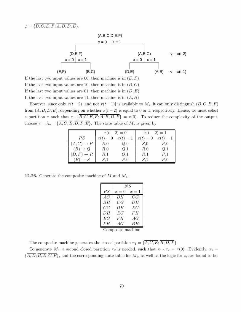
ϕ = {B,C,E, F ;A,B,D,E}.
x = 0
(A,B,C,D,E,F)
x = 1
x = 1x = 0x = 1x = 0
(A,B,C)(D,E,F)
(E,F) (A,B)(D,E)(B,C)
x(t-2)
x(t-1)
If the last two input values are 00, then machine is in (E,F )
If the last two input values are 10, then machine is in (B,C)
If the last two input values are 01, then machine is in (D,E)
If the last two input values are 11, then machine is in (A,B)
However, since only x(t− 2) [and not x(t− 1)] is available to Ms, it can only distinguish (B,C,E, F )
from (A,B,D,E), depending on whether x(t− 2) is equal to 0 or 1, respectively. Hence, we must select
a partition τ such that τ · {B,C,E, F ;A,B,D,E} = π(0). To reduce the complexity of the output,
choose τ = λo = {A,C ;B;D,F ;E}. The state table of Ms is given by
x(t − 2) = 0 x(t − 2) = 1PS x(t) = 0 x(t) = 1 x(t) = 0 x(t) = 1
(A,C) → P R,0 Q,0 S,0 P ,0(B) → Q R,0 Q,1 R,0 Q,1
(D,F ) → R R,1 Q,1 R,1 P ,1(E) → S S,1 P ,0 S,1 P ,0
12.26. Generate the composite machine of M and Ma.
NSPS x = 0 x = 1
AG BH CGBH CG DHCG DH EGDH EG FHEG FH AGFH AG BH
Composite machine
The composite machine generates the closed partition π1 = {A,C,E;B,D,F}.To generate Mb, a second closed partition π2 is needed, such that π1 · π2 = π(0). Evidently, π2 =
{A,D;B,E;C,F}, and the corresponding state table for Mb, as well as the logic for z, are found to be:
70
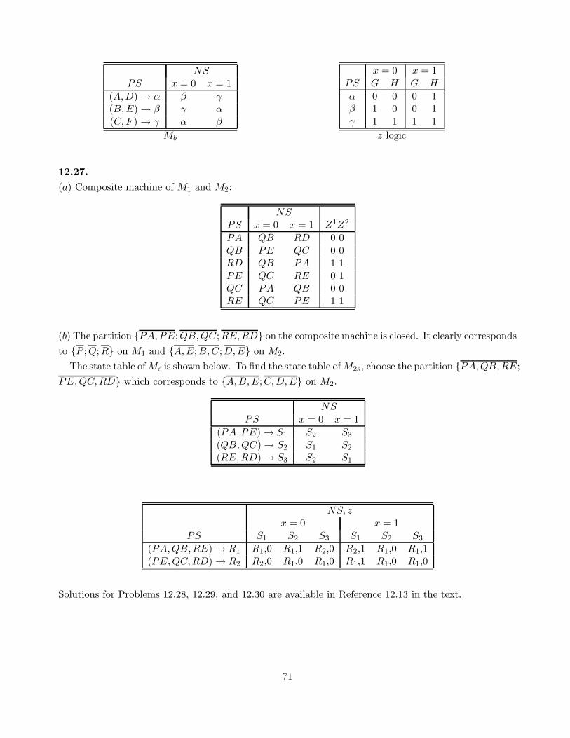
NSPS x = 0 x = 1
(A,D) → α β γ(B,E) → β γ α(C,F ) → γ α β
Mb
x = 0 x = 1PS G H G H
α 0 0 0 1β 1 0 0 1γ 1 1 1 1
z logic
12.27.
(a) Composite machine of M1 and M2:
NSPS x = 0 x = 1 Z1Z2
PA QB RD 0 0QB PE QC 0 0RD QB PA 1 1PE QC RE 0 1QC PA QB 0 0RE QC PE 1 1
(b) The partition {PA,PE;QB,QC;RE,RD} on the composite machine is closed. It clearly corresponds
to {P ;Q;R} on M1 and {A,E;B,C;D,E} on M2.
The state table of Mc is shown below. To find the state table of M2s, choose the partition {PA,QB,RE;
PE,QC,RD} which corresponds to {A,B,E;C,D,E} on M2.
NSPS x = 0 x = 1
(PA,PE) → S1 S2 S3
(QB,QC) → S2 S1 S2
(RE,RD) → S3 S2 S1
NS, zx = 0 x = 1
PS S1 S2 S3 S1 S2 S3
(PA,QB,RE) → R1 R1,0 R1,1 R2,0 R2,1 R1,0 R1,1(PE,QC,RD) → R2 R2,0 R1,0 R1,0 R1,1 R1,0 R1,0
Solutions for Problems 12.28, 12.29, and 12.30 are available in Reference 12.13 in the text.
71

Chapter 13
13.1.
(a) Shortest homing sequences:
M1: 000,011,110,111
M2: 01
M3: 00,01
(b) Shortest synchronizing sequences:
M1: 000 (to state A).
M2: 000 (to B), 111 (to A).
M3: 01010 (to C).
13.2. If one precludes taking adaptive decisions in which a new input symbol is applied after looking
at the previous output symbols, then the procedure is simply that of deriving a synchronizing sequence.
A minimal synchronizing sequence is 00101000. The corresponding path through the synchronizing tree
is shown below.
(ABCDEF )0→ (ABCEF )
0→ (ABCE)
1→ (DEF )
0→ (BF )
1→ (CD)
0→ (EF )
0→ (B)
0→ (A)
If an adaptive experiment is allowed, then the minimal homing sequence 001 can be first derived. Then
depending on the response to this homing sequence, as shown in the table below, a transfer sequence
can be used to reach state A. This requires only five input symbols in the worst case.Response to homing sequence 001
Initial Response to Final Transfer
state 001 state sequence
A 100 F T (F,A) = 00B 011 D T (D,A) = 1C 011 D T (D,A) = 1D 111 D T (D,A) = 1E 101 E T (E,A) = 00F 101 E T (E,A) = 00
13.3.
(i) Form the direct sum of the two machines. (ii) Construct a preset homing experiment that will
determine the machine at the end of the experiment.
NS,z
PS x = 0 x = 1
A A, 0 B, 0B C, 0 A, 0C A, 1 B, 0D E, 0 F, 1E F, 0 D, 0F E, 0 F, 0
Direct sum
72
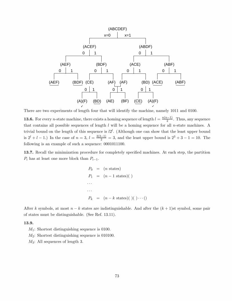
0
x=0
(ABCDEF)
0
x=1
(ABDF)(ACEF)
(ACE) (ABF)
(ACE) (ABF)
1
1
0
(AF) (BD)
1
0
(AE) (BF)
1 0 1
0
(AEF) (BDF)
1
0 1
0 1
(CE) (A)(F)(BD)
(BDF)(AEF)
(A)(F)
0
(CE) (AF)
1
There are two experiments of length four that will identify the machine, namely 1011 and 0100.
13.6. For every n-state machine, there exists a homing sequence of length l = n(n−1)2 . Thus, any sequence
that contains all possible sequences of length l will be a homing sequence for all n-state machines. A
trivial bound on the length of this sequence is l2l. (Although one can show that the least upper bound
is 2l + l − 1.) In the case of n = 3, l = 3(3−1)2 = 3, and the least upper bound is 23 + 3 − 1 = 10. The
following is an example of such a sequence: 0001011100.
13.7. Recall the minimization procedure for completely specified machines. At each step, the partition
Pi has at least one more block than Pi−1.
P0 = (n states)
P1 = (n − 1 states)( )
· · ·· · ·Pk = (n − k states)( )( ) · · · ()
After k symbols, at most n − k states are indistinguishable. And after the (k + 1)st symbol, some pair
of states must be distinguishable. (See Ref. 13.11).
13.9.
M1: Shortest distinguishing sequence is 0100.
M2: Shortest distinguishing sequence is 010100.
M3: All sequences of length 3.
73
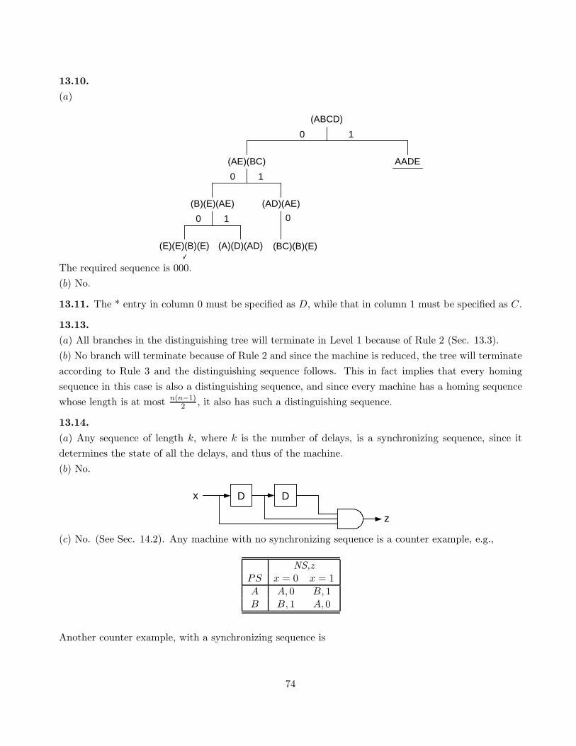
13.10.
(a)
0
0
(ABCD)
0
1
AADE(AE)(BC)
(B)(E)(AE)
(BC)(B)(E)
(AD)(AE)
(E)(E)(B)(E) (A)(D)(AD)
1
1
0
The required sequence is 000.
(b) No.
13.11. The * entry in column 0 must be specified as D, while that in column 1 must be specified as C.
13.13.
(a) All branches in the distinguishing tree will terminate in Level 1 because of Rule 2 (Sec. 13.3).
(b) No branch will terminate because of Rule 2 and since the machine is reduced, the tree will terminate
according to Rule 3 and the distinguishing sequence follows. This in fact implies that every homing
sequence in this case is also a distinguishing sequence, and since every machine has a homing sequence
whose length is at most n(n−1)2 , it also has such a distinguishing sequence.
13.14.
(a) Any sequence of length k, where k is the number of delays, is a synchronizing sequence, since it
determines the state of all the delays, and thus of the machine.
(b) No.
Dx
z
D
(c) No. (See Sec. 14.2). Any machine with no synchronizing sequence is a counter example, e.g.,
NS,z
PS x = 0 x = 1
A A, 0 B, 1B B, 1 A, 0
Another counter example, with a synchronizing sequence is
74

NS
PS x = 0 x = 1
A A BB B B
13.16. 01 is a homing sequence for the machine in question. A response 10 indicates a final state B.
The first 1 symbol of the next input sequence takes the machine to state A; the correct output symbol
is 0. It is easy to verify that the rest of the sequence takes the machine through every transition and
verifies its correctness. The correct output and state sequences are:
X : 0 1 0 1 0 1 0 1A A B C C B A A B
Z : 1 0 0 1 0 0 1 0
X : 0 0 1 0 0 1 1 0B C B A A A B A A
Z : 0 0 0 1 1 0 0 1
X : 1 0 0 0 1A B C B C C
Z : 0 0 0 0 1
13.18. The state table for which the given experiment is a checking experiment is
NS,z
PS x = 0 x = 1
A B, 0 B, 1B C, 1 D, 1C A, 2 A, 1D E, 3 A, 2E D, 3 B, 2
If the shortest distinguishing prefix of the distinguishing sequence 010 is used to identify the states, the
given checking experiment can be obtained. The shortest distinguishing prefixes and the corresponding
responses are summarized below:
Initial Shortest Response to shortest Final
state distinguishing prefix distinguishing prefix state
A 0 0 BB 0 1 CC 0 2 AD 010 321 CE 010 320 B
13.19. The sequence 000 is a synchronizing sequence (to state D). Both 000 and 111 are distinguishing
75

sequences. To perform the experiment, apply 000 first and regardless of the machine’s response to this
sequence, construct, in the usual manner, a checking experiment, using the shortest distinguishing prefix
of either distinguishing sequence. An experiment that requires 25 symbols is given below:
X : 0 0 0 0 0 1 0 0− − − D D D A D D
Z : − − − 1 1 1 0 1
X : 1 1 0 0 0 1 1 1D A C A D D A C B
Z : 1 0 0 0 1 1 0 0
X : 0 0 0 0 1 1 1 1 0B C A D D A C B D D
Z : 0 0 0 1 1 0 0 0 1
13.20. The given sequences do not constitute a checking experiment, since the response in question can
be produced by the two distinct machines shown below.
NS,z
PS x = 0 x = 1
A A, 2 B, 2B C, 0 A, 1C D, 1 E, 0D E, 2 A, 0E B, 1 C, 2
Machine M∗
NS,z
PS x = 0 x = 1
1 1, 2 3, 22 5, 1 2, 23 4, 0 1, 04 3, 1 2, 05 2, 2 1, 1
Machine M
Input : 0 0 1 0 0 1 0 1State in M 1 1 1 3 4 3 1 1 3State in M∗ A A A B C D A A BOutput : 2 2 2 0 1 0 2 2
Input : 0 1 1 0 0 0 1 0 0State in M 3 4 2 2 5 2 5 1 1 1State in M∗ B C E C D E B A A AZ : 0 0 2 1 2 1 1 2 2
(Actually, there exist eight distinct, five-state machines which produce the above output sequence in
response to the given input sequence.)
13.21.
(a) The distinguishing sequences are: 00, 01.
76

Response to Initial
00 state
00 A01 B11 C10 D
Response to Initial
01 state
00 A01 B11 C or D10 D or C
(b)
NS,z
PS x = 0 x = 1
A B, 0 B, 0B C, 0 C, 0C D, 1 D, 1D A, 1 D, 1
OR
NS,z
PS x = 0 x = 1
A B, 0 C, 1B C, 0 D, 0C D, 1 C, 1D A, 1 B, 0
13.23
(a)
BC
AD
AB CD
BD AC
1/01/0
1/01/0
1/0
1/0
(b)
NS, zz1
PS x = 0 x = 1
A A, 0φ B, 01B A, 0φ C, 00C A, 0φ D, 00D A, 1φ A, 01
(c) Assuming an initial state A and all don’t-care combinations equal to 0, we obtain the following
checking experiment.
X : 1 1 1 1 1 1 0 1 1 1 0 1Z : 2 0 0 2 0 0 0 2 0 0 1 2
77

X : 1 1 1 0 1 1 1 1 1 0 1 1Z : 0 0 2 0 2 0 0 2 0 0 2 0
(Note that an output symbol 2 is used to denote 10, 1 to denote 01, and 0 to denote 00.)
13.24. Let S(t) denote the state at time t, that is, just before the application of the tth input symbol
(e.g., the initial state is S(1)). There seems to be no input sequence that yields three different responses
at three different points in the experiment. Thus, more sophisticated reasoning must be used.
To begin with, the machine has at least one state that responds to input symbol 0 by producing an
output symbol 1. Consequently, the machine has at most two states that respond to an input symbol
0 by producing an output symbol 0. Now consider the portion of the experiment between t = 4 and
t = 11. Each of the states S(4), S(6), and S(8) respond to a 0 by producing a 0. However, at most
two of these states can be distinct. Therefore, either S(4) = S(6) or S(4) = S(8) or S(6) = S(8). If
S(4) = S(6), then S(6) = S(8); thus S(8) is identical to either S(4) or S(6). This in turn implies that
S(10) is identical to either S(6) or S(8). Therefore S(10) is a state that responds to an input symbol 0
by producing an output symbol 0, and to an input symbol 1 by producing an output symbol 1.
Using similar reasoning, when examining the portion of the experiment between t = 14 and t = 18,
we conclude that S(17) must be identical to either S(15) or S(16). Thus, S(17) is a state that responds
to a 0 by producing a 0, and to a 1 by producing a 0. Therefore, the circuit does have two distinct
states that respond to a 0 by producing a 0: S(10) and S(17).
A careful analysis of the experiment yields the state table below:
NS,z
PS x = 0 x = 1
A B, 0 C, 1B B, 0 A, 0C C, 1 A, 0
13.25.
(a) For each fault-free state transition, there are three possible SST faults. The collapsed set of SSTs for
each such transition is given in the following table. The collapsed set is not unique, but is of minimum
cardinality. For fault collapsing, we use the fact that:
SPDS(A,B) = SPDS(A,C) = SPDS(B,D) = SPDS(C,D) = 0
SPDS(A,B) = SPDS(A,D) = SPDS(B,C) = SPDS(C,D) = 1
78

Fault-free transition Set of collapsed faults
< 0, A,C, 0 > < 0, A,A, 0 >, < 0, A,B, 0 >< 1, A,C, 0 > < 1, A,A, 0 >, < 1, A,B, 0 >< 0, B,C, 1 > < 0, B,A, 1 >, < 0, B,B, 1 >< 1, B,B, 1 > < 1, B,A, 1 >, < 1, B,D, 1 >< 0, C,D, 1 > < 0, C,A, 1 >, < 0, C,B, 1 >< 1, C,A, 0 > < 1, C,B, 0 >, < 1, C,D, 0 >< 0,D,A, 0 > < 0,D,B, 0 >, < 0,D,D, 0 >< 1,D,B, 1 > < 1,D,A, 1 >, < 1,D,C, 1 >
Whenever both 0 and 1 are available as SPDS of a pair of states, we assume in the above table that 0
is used as SPDS.
(b) To derive a test sequence for this SST fault, we first need T (A,B) = 001 or 101. Then the activation
vector x = 1 is applied. Finally, SPDS(B,C) = 1 is applied. Hence, one possible test sequence is 00111.
13.27.
(a) A minimal test set: (x1, x2, y1, y2) = {(0,0,1,1), (1,1,0,0), (1,1,1,1)}.(b) Minimum no. of clock cycles: 3(2 + 1) + 2 − 1 = 10.
13.30. The three-stage LFSR for the polynomial x3 + x + 1 is shown below. Its state sequence that
repeats on y1y2y3 (not on y3y2y1 as in Fig. 13.16) is: 111 → 101 → 001 → 010 → 100 → 011 → 110.
This is exactly the reverse of the cycle shown in Fig. 13.16 for the polynomial x3 + x2 + 1.
D +Y3
y3 Y2 Y1y2 y1
DD
13.31. Test set: (x3, x2, x1) = {(0,1,1), (1,0,0), (0,1,0), (0,0,1)}.
79

Chapter 14
14.1.
(a) Not finite memory
(b) Finite memory of order 3.
(c) Finite memory of maximal order, that is, µ = 5(5−1)2 = 10.
14.2. The machine in question can be shown to be finite memory of order 2. Let us determine the
information supplied by the “input” and “output” delay registers. The synchronizing tree is shown
below:
x=0
(ABCD)
x=1
(ABCD) (ABCD)
It clearly supplies no information, and thus the input delays are redundant in this case. The output
synchronizing tree is shown below.
z=0
(ABCD)
z=1
(BD)(AC)
A DCB
z=0z=0 z=1z=1
From the above tree, it is evident that the machine in question can be realized in the form:
zCombinational logic
D
x
z1
D
1
z2z1x 00 01 11 10
1
0
1
0
0
0
0
11
z = x z2
The map of the combinational logic reveals that it is independent of the value of z1.
14.4. The canonical realization of a finite-memory machine, shown in Fig. P14.2, has (p)µ · (q)µ = (pq)µ
states. (Note that the input delay register may have (p)µ output combinations, etc.). If such a realization
corresponds to a finite-memory n-state machine, then clearly (pq)µ ≥ n.
14.5. The machine in question is definite of order µ = 3. The canonical realization and combinational
logic are shown below.
80
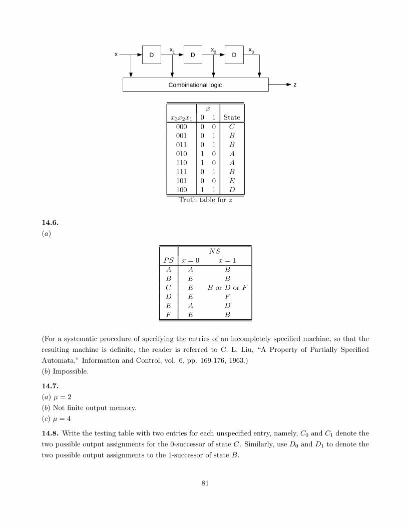
zCombinational logic
xx1D D D
x3x2
xx3x2x1 0 1 State
000 0 0 C001 0 1 B011 0 1 B010 1 0 A110 1 0 A111 0 1 B101 0 0 E100 1 1 D
Truth table for z
14.6.
(a)
NSPS x = 0 x = 1
A A BB E BC E B or D or FD E FE A DF E B
(For a systematic procedure of specifying the entries of an incompletely specified machine, so that the
resulting machine is definite, the reader is referred to C. L. Liu, “A Property of Partially Specified
Automata,” Information and Control, vol. 6, pp. 169-176, 1963.)
(b) Impossible.
14.7.
(a) µ = 2
(b) Not finite output memory.
(c) µ = 4
14.8. Write the testing table with two entries for each unspecified entry, namely, C0 and C1 denote the
two possible output assignments for the 0-successor of state C. Similarly, use D0 and D1 to denote the
two possible output assignments to the 1-successor of state B.
81

PS 0/0 0/1 1/0 1/1
A B – – CB D – D0 D1
C C0 C1 A –D C – – A
AB BD – – CD1
AC BC0 – – –AD BC – – ACBC C0D – AD0 –BD CD – – AD1
CD CC0 – – –
AB BD AD
CD
D1
BC AC
D0
D1
C0C0
From the testing graph, it is evident that D0 results in a loop and must be eliminated. Consequently,
D1 must be selected. It is also evident that C0 results in the longest path, i.e., l = 5 and µ = 6.
14.10.
(a) Test the output successor table, whose entries must all be single-valued, for definiteness.
(b) See machine in Fig. P14.2. Its output successor table is definite of order µ = 2.
14.11.
(a) Lossy, since D implies (AC), which implies (BC), which in turn implies (AA).
(b) The machine has three compatible pairs, as shown by the testing graph below. Since the graph is
not loop-free, the machine is lossless of infinite order.
AB CD
EF
1
100
(c) Machine is lossless of order µ = 3.
(d) Machine is lossy, since (DE) implies (EE).
14.14. In rows C and D, column x = 0, output symbol should be 11. In row B, column x = 1, output
symbol should be 10. Such a (unique) specification yields a lossless machine of order µ = 4.
82

14.16.
(a) If we disregard z2 and consider the machine with output z1 only, we can show that it is information
lossless. Consequently, the input sequence X can always be retrieved from the output sequence Z1 and
the initial and final states. In this case, the input sequence can be determined from the output successor
and output predecessor tables, i.e., X = 011011.
The determination of z2 for the given X is straightforward, i.e., Z2 = 010010.
(b) Yes, by using the foregoing procedure.
14.18.
(a) From the output sequence Z and the final state of M2, we shall determine (by performing backward
tracing) the intermediate sequence Y . From Y , by means of the output predecessor table of M1, we
shall determine the initial state of M1. The state sequence of M2 and the Y sequence are obtained from
the output predecessor table of M2.
z = 0 z = 1 NS
B, 0 C, 1 AA, 0 D, 0 BB, 1 A, 1 CD, 1 C, 0 D
Y : 1 1 0 1 0 0A C A B C D B
Z : 1 1 0 0 1 1
The state sequence of M1 is obtained from the output predecessor table of M1 as follows.
y = 0 y = 1 NS
– D AA B BB A C
(CD) – D
A A AA A
A B B BD C B
D C C CD D
D D Dy = 1 1 0 1 0 0
The initial state of M1 is thus D. The input sequence X is either 110100 or 111100.
83

(b) From the output predecessor table of M2, it is obvious that, given the output sequence Z and final
state of M2, we can always determine the input sequence Y . And since M1 can be shown to be finite
output memory of length µ = L = 6, the statement is proved.
14.19. To determine the initial state of M2, we must determine its distinguishing sequences. These
sequences should then be produced as output sequences by M1. The distinguishing tree for M2 is:
0
0
(DEFG)
0
1
(DDGE)(DEF)
(DEF) (DEG)
(EF) (DDG)
1
1
0
(DF) (EG)
1
0
(F)F) (DG)
1
The shortest distinguishing sequence for M2 is: 01010. Now, perform backward tracing on the output
successor of M1 to determine which input sequence X will yield Y = 01010.
NS, xPS y = 0 y = 1
A (B, 0) (C, 1)B (A, 1) (C, 0)C (A, 0)(B, 1) −
From the output successor table, we find that X can be any one of the following sequences: 00010,
00011, 00100, 00101.
14.20. (a) From the output predecessor table shown below, we find the following state and input
sequences:
PS, xz = 0 z = 1 NS
B, 0 C, 1 AA, 0 D, 0 BB, 1 A, 1 CD, 1 C, 0 D
84

Input : 1 0 1 0 0State : C A B C D BOutput : 1 0 0 1 1
(b) The proof is evident when we observe that all the entries of the output predecessor table are single-
valued and the two transitions in each row are associated with different values of x.
(c) Use output predecessor tables and generalize the arguments in (b). It may be helpful to define a
“lossless” output predecessor table of the µth order.
14.21.
(a) The output successor and predecessor tables are shown as follows:
PS z = 0 z = 1
A C BB − BDC B ED AE −E F DF D A
Output successor table
z = 0 z = 1 NS
D F AC AB BA − CF BE DD C EE − F
Output predecessor table
Following the procedure for retrieving the input sequence, illustrated in Fig. 14.11, we find
Successors to A A B
1
Predecessors to F
Z
State sequence
Input sequence
BD
AE
BD
CF
CF
BD
CF
AE
AE
AB
AB
BE
ED F CD FEA
A B B ED F CD FEA
00 0100011
0 10 0000001
(b) No, since the 11011000-successor of A may be either B or D, but not A.
14.23. The machine is lossless of order µ = 2. Hence, the inverse state can be defined by the initial
state and one successor output symbol. The possible states are (A, 1); (B, 0); (C, 1); (D, 0); (E, 1);
(F, 0). The state table for the inverse machine is as follows.
85
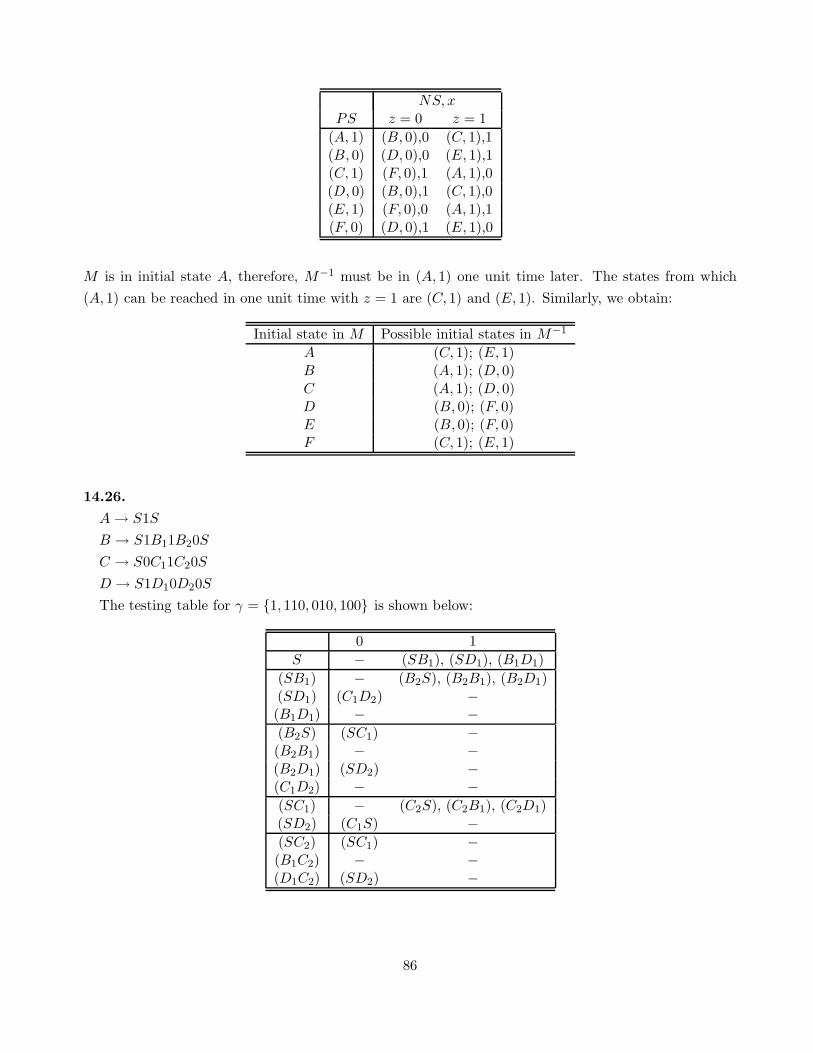
NS, xPS z = 0 z = 1
(A, 1) (B, 0),0 (C, 1),1(B, 0) (D, 0),0 (E, 1),1(C, 1) (F, 0),1 (A, 1),0(D, 0) (B, 0),1 (C, 1),0(E, 1) (F, 0),0 (A, 1),1(F, 0) (D, 0),1 (E, 1),0
M is in initial state A, therefore, M−1 must be in (A, 1) one unit time later. The states from which
(A, 1) can be reached in one unit time with z = 1 are (C, 1) and (E, 1). Similarly, we obtain:
Initial state in M Possible initial states in M−1
A (C, 1); (E, 1)B (A, 1); (D, 0)C (A, 1); (D, 0)D (B, 0); (F, 0)E (B, 0); (F, 0)F (C, 1); (E, 1)
14.26.
A → S1S
B → S1B11B20S
C → S0C11C20S
D → S1D10D20S
The testing table for γ = {1, 110, 010, 100} is shown below:
0 1
S − (SB1), (SD1), (B1D1)
(SB1) − (B2S), (B2B1), (B2D1)(SD1) (C1D2) −(B1D1) − −(B2S) (SC1) −(B2B1) − −(B2D1) (SD2) −(C1D2) − −(SC1) − (C2S), (C2B1), (C2D1)(SD2) (C1S) −(SC2) (SC1) −(B1C2) − −(D1C2) (SD2) −
86

Since the pair (SS) was not generated in the table, the code is uniquely decipherable. Let us now
construct the testing graph to determine the delay µ
S
B1D1
1
SD1
SB1
1
1
SB2
C1D2
SC11
0
0
B1B2
B2D1
1
1
SD2
0
B1C2
C2D1
SC2
1
1
1
0
0
0
The graph is clearly not loop-free; one of the loops being (SC1) → (SC2) → (SC1). The infinite
message 1101010· · · cannot be deciphered in a finite time, since it can be interpreted as AACACAC · · ·or BACAC · · ·.
14.27. Following the deciphering procedure in Fig. 14.16 we find
0 0 , 1 , 0 , 1 , 0 0 , 1 , 1 0 , 1 0 , 0 , 1 1 , 0 0 , 0 , 1, ,, ,
, ,,,
,,,
, ,,
The message is 0; 0; 101; 001; 101; 0; 011; 0; 001.
87

Chapter 15
15.1.
(a)
xc
+
+
xb
xa za
zb
zc
(b)
za : 0 1 0 1 1 1 1 0 0 0 1 0 1 1zb : 1 0 0 0 1 1 1 0 1 0 0 1 1 0zc : 1 1 1 0 0 1 1 0 0 0 1 1 0 0
(c)
xa = za
xb = za + zb
xc = za + zb + zc
15.2.
(a)
T = zx
= 1 + D + D3 + D4 + D5 (modulo 2)
(b)
(1 + D + D3 + D4 + D5)X0 = 0
X0 = (D + D3 + D4 + D5)X0
X0 : (00001)1100110111110100010010101100001
The sequence consists of 31 symbols, and thus it is maximal. (Note that 25 − 1 = 31.)
(c)
T−1 = 11+D+D3+D4+D5
x z+ + + +
15.5. The transfer function of the left circuit is
T1 = D3 + 1
while that of the right circuit is
T2 = (D2 + 2D + 1)(D + 1)
88

However,
T2 = (D2 + 2D + 1)(D + 1) = D3 + D2 + 2D2 + 2D + D + 1 = D3 + 1 = T1
15.6. Proof is obvious, using the identity
(1 + 2D)−1 = 1 + 14D + 4D2 + 8D2 (modulo 16)
15.7.
(2D3 + D2 + 2)X0 = 0
2D3X0 + D2X0 = X0
Thus, the present digit of the null sequence is equal to the modulo-3 sum of the second previous digit
and the third previous digit. The sequence
(001) 0 1 2 1 1 2 0 1 1 1 0 0 2 0 2 1 2 2 1 0 2 2 2 0 0 1
is the desired null sequence. It is a maximal sequence, since it contains all 33 − 1 = 26 possible nonzero
subsequences of three ternary digits.
15.8. Proof can be found in Reference 15.10 or Reference 15.14, pp. 72-73.
15.9.
x z+ + 2
2
+ Y1 Y3Y2y1 y3y2
z = DY3 = D(2x + 2y2) = 2Dx + 2Dy2 (1)
y2 = DY2 = D(y1 + x) = D(DY1 + x) = D2Y1 + DX (2)
Y1 = x + 2y2 = x + 2D2Y1 + 2Dx (3)
Eq. (3) can be rewritten as
Y1 + D2Y1 = x + 2Dx
or
Y1 =x(1 + 2D)
1 + D2(4)
Substituting Eq. (4) into Eq. (2), we obtain
y2 =x(D2 + 2D3)
1 + D2+ Dx (5)
Substituting Eq. (5) into Eq. (1), we have
z = 2Dx + 2D2x +2Dx(D2 + 2D3)
1 + D2
89

Thus,
T =z
x=
2D + 2D2 + D3
1 + D2
15.10.
(a)
T = T1 + T1T2T1 + T1T2T1T2T1 + T1T2T1T2T1T2T1 + · · ·= T1[1 + T1T2 + (T1T2)
2 + (T1T2)3 + · · ·]
=T1
1 − T1T2
(b)
T = 2D +2D2
1 − 2D2+
2D3
1 − 2D2
=2D + 2D3 + 2D2 + 2D3
1 + D2
=2D + 2D2 + D3
1 + D2
15.11. The transfer function is
T =1 + D
1 + D2 + D3
15.12.
(b) Impulse responses:
for T1: (1101001)· · ·for T2: 0(01220211)· · ·
The sequences in parenthesis repeat periodically.
(c) T1 has a delayless inverse
T−11 =
1 + D + D3
1 + D2
T2 has no constant term in its numerator, consequently it does not have an instantaneous inverse. It
does, however, have a delayed inverse.
15.13.
(a) It can be shown, by the Euclidean algorithm, that the greatest common divisor to the numerator
and denominator is D2 + D + 1. Thus,
D7 + D4 + D2 + D + 1 = (D2 + D + 1)(D5 + D4 + 1)
D10 + D9 + D8 + D7 + D = (D2 + D + 1)(D8 + D5 + D4 + D2 + D)
So that
T =D8 + D5 + D4 + D2 + D
D5 + D4 + 1
90
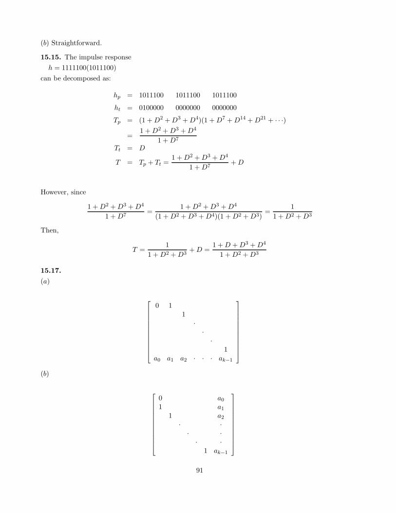
(b) Straightforward.
15.15. The impulse response
h = 1111100(1011100)
can be decomposed as:
hp = 1011100 1011100 1011100
ht = 0100000 0000000 0000000
Tp = (1 + D2 + D3 + D4)(1 + D7 + D14 + D21 + · · ·)
=1 + D2 + D3 + D4
1 + D7
Tt = D
T = Tp + Tt =1 + D2 + D3 + D4
1 + D7+ D
However, since
1 + D2 + D3 + D4
1 + D7=
1 + D2 + D3 + D4
(1 + D2 + D3 + D4)(1 + D2 + D3)=
1
1 + D2 + D3
Then,
T =1
1 + D2 + D3+ D =
1 + D + D3 + D4
1 + D2 + D3
15.17.
(a)
0 11
··
·1
a0 a1 a2 · · · ak−1
(b)
0 a0
1 a1
1 a2
· ·· ·
· ·1 ak−1
91
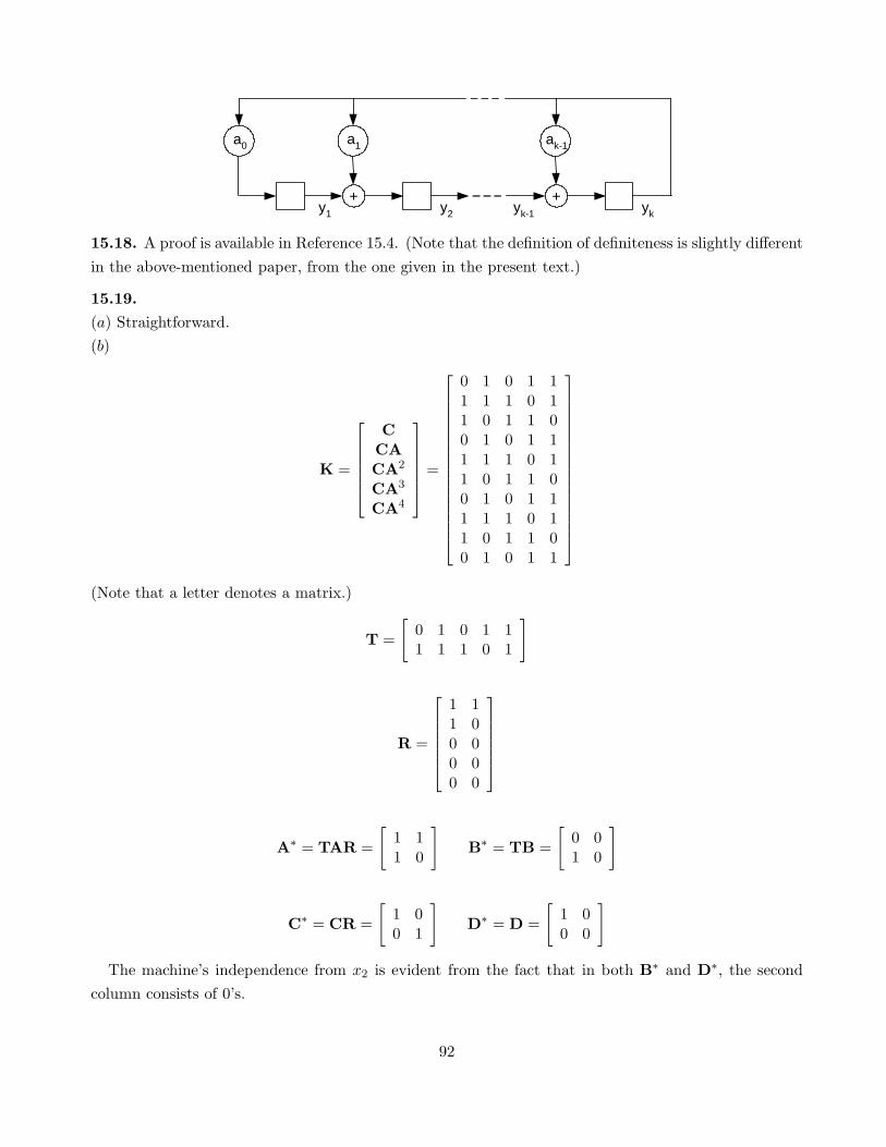
+yky2
a1a0
+y1
ak-1
yk-1
15.18. A proof is available in Reference 15.4. (Note that the definition of definiteness is slightly different
in the above-mentioned paper, from the one given in the present text.)
15.19.
(a) Straightforward.
(b)
K =
CCACA2
CA3
CA4
=
0 1 0 1 11 1 1 0 11 0 1 1 00 1 0 1 11 1 1 0 11 0 1 1 00 1 0 1 11 1 1 0 11 0 1 1 00 1 0 1 1
(Note that a letter denotes a matrix.)
T =
[
0 1 0 1 11 1 1 0 1
]
R =
1 11 00 00 00 0
A∗ = TAR =
[
1 11 0
]
B∗ = TB =
[
0 01 0
]
C∗ = CR =
[
1 00 1
]
D∗ = D =
[
1 00 0
]
The machine’s independence from x2 is evident from the fact that in both B∗ and D∗, the second
column consists of 0’s.
92

15.20.
K4 =
z(0)z(1)z(2)z(3)
=
1 0 1 01 0 0 11 0 1 01 0 0 1
Clearly, the rank of K4 is two, and thus
T =
[
1 0 1 01 0 0 1
]
R =
0 10 01 10 0
Therefore,
A∗ = TAR =
[
0 11 0
]
B∗ = TB =
[
01
]
C∗ = CR =[
1 0]
D∗ = D =[
0]
The schematic diagram of the reduced linear machine is shown below:
x z+
15.21.
(a) Straightforward.
(b)
K3 =
CCACA2
=
1 1 01 1 11 1 10 1 10 1 10 0 0
The rank of K3 is 3; hence no reduction in the machine’s dimension is possible.
T =
1 1 01 1 10 1 1
R =
0 1 11 1 11 1 0
A∗ = TAR =
0 1 00 0 10 0 0
B∗ = TB =
001
C∗ = CR =
[
1 0 00 1 0
]
D∗ = D =
[
01
]
93
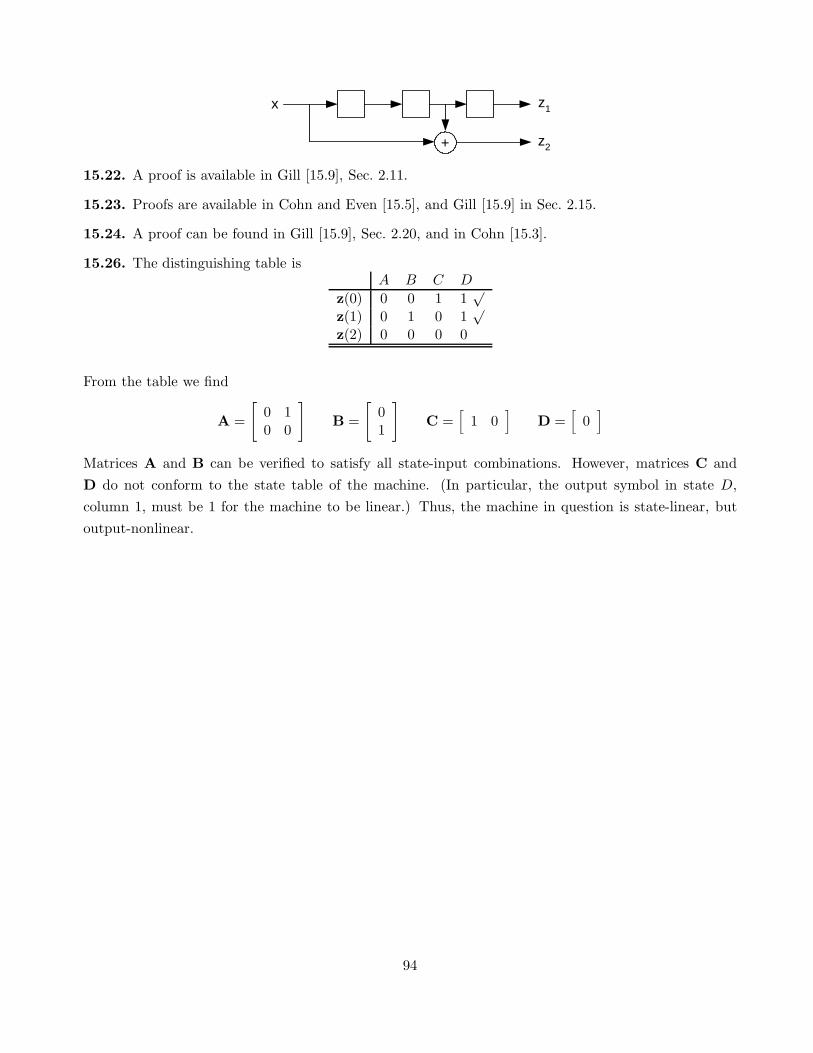
x z1
+ z2
15.22. A proof is available in Gill [15.9], Sec. 2.11.
15.23. Proofs are available in Cohn and Even [15.5], and Gill [15.9] in Sec. 2.15.
15.24. A proof can be found in Gill [15.9], Sec. 2.20, and in Cohn [15.3].
15.26. The distinguishing table isA B C D
z(0) 0 0 1 1√
z(1) 0 1 0 1√
z(2) 0 0 0 0
From the table we find
A =
[
0 10 0
]
B =
[
01
]
C =[
1 0]
D =[
0]
Matrices A and B can be verified to satisfy all state-input combinations. However, matrices C and
D do not conform to the state table of the machine. (In particular, the output symbol in state D,
column 1, must be 1 for the machine to be linear.) Thus, the machine in question is state-linear, but
output-nonlinear.
94
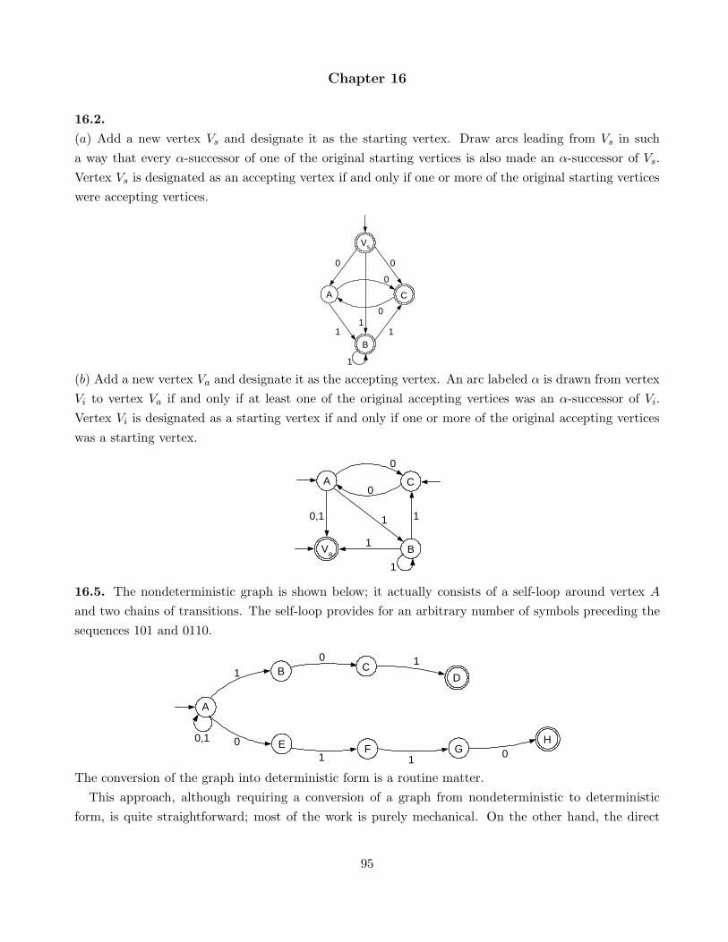
Chapter 16
16.2.
(a) Add a new vertex Vs and designate it as the starting vertex. Draw arcs leading from Vs in such
a way that every α-successor of one of the original starting vertices is also made an α-successor of Vs.
Vertex Vs is designated as an accepting vertex if and only if one or more of the original starting vertices
were accepting vertices.
A C
Vs
0
0
1 1B
1
0 0
1
(b) Add a new vertex Va and designate it as the accepting vertex. An arc labeled α is drawn from vertex
Vi to vertex Va if and only if at least one of the original accepting vertices was an α-successor of Vi.
Vertex Vi is designated as a starting vertex if and only if one or more of the original accepting vertices
was a starting vertex.
A C
Va
0
0
0,1 1
B
1
1
1
16.5. The nondeterministic graph is shown below; it actually consists of a self-loop around vertex A
and two chains of transitions. The self-loop provides for an arbitrary number of symbols preceding the
sequences 101 and 0110.
G
B1
0,1 0 E
1
F
C
01
A
0
1
D
H
The conversion of the graph into deterministic form is a routine matter.
This approach, although requiring a conversion of a graph from nondeterministic to deterministic
form, is quite straightforward; most of the work is purely mechanical. On the other hand, the direct
95
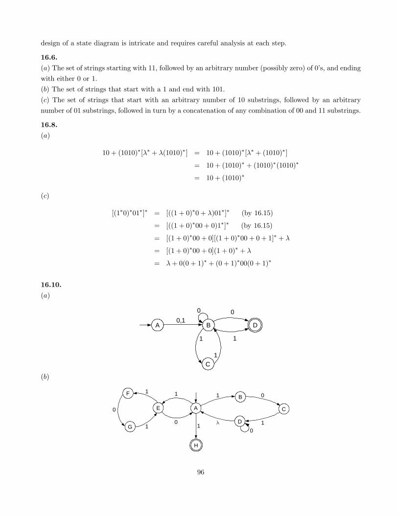
design of a state diagram is intricate and requires careful analysis at each step.
16.6.
(a) The set of strings starting with 11, followed by an arbitrary number (possibly zero) of 0’s, and ending
with either 0 or 1.
(b) The set of strings that start with a 1 and end with 101.
(c) The set of strings that start with an arbitrary number of 10 substrings, followed by an arbitrary
number of 01 substrings, followed in turn by a concatenation of any combination of 00 and 11 substrings.
16.8.
(a)
10 + (1010)∗[λ∗ + λ(1010)∗] = 10 + (1010)∗[λ∗ + (1010)∗]
= 10 + (1010)∗ + (1010)∗(1010)∗
= 10 + (1010)∗
(c)
[(1∗0)∗01∗]∗ = [((1 + 0)∗0 + λ)01∗]∗ (by 16.15)
= [((1 + 0)∗00 + 0)1∗]∗ (by 16.15)
= [(1 + 0)∗00 + 0][(1 + 0)∗00 + 0 + 1]∗ + λ
= [(1 + 0)∗00 + 0](1 + 0)∗ + λ
= λ + 0(0 + 1)∗ + (0 + 1)∗00(0 + 1)∗
16.10.
(a)
C
0
1
A0,1
B D
1
1
0
(b)
A
1
B 0
C
H
1
10
E
0 D
11
1
F
G
0
96

(c)
B
1
C F
0
1 0
A
D
E
1
1
0
1
16.15. Only the set described in (b) is regular, since in all other cases, a machine that recognizes the set
in question must be capable of counting an arbitrary number of 1’s – a task that no finite-state machine
can accomplish.
16.17.
(a) The reverse of an expression that contains no star operations is simply the expression written
backwards. For example, the reverse of (10+1)01(011+10) is (01+110)10(1+01). The reverse of the set
A∗ is (Ar)∗. For example, the reverse of (1 + 01∗)∗ is (1∗0 + 1)∗. Thus, the reverse Rr of a regular
expression R can be obtained by shifting each star immediately to the left of the subexpression to which
it applies and reversing the resulting expression
(b) Rr = (0∗11∗0)∗0∗1 + (0∗1 + 0)∗(00)∗
16.18.
(a) Yes, since every finite set of strings is regular and can be recognized by a finite-state machine.
(b) No. Since, for example, P does not contain the string λ.
(c) No. Let R denote the set of all strings (0+1)∗ . Clearly, the set of palindromes is a subset of (0+1)∗,
but is not regular (see Problem 10.3).
(d) No. See answer to (c).
16.21. Let M be the finite-state machine whose state diagram is shown below (assuming an alphabet
{0,1}). Suppose that M receives its input from another finite-state machine whose outputs are strings
from P . If the inputs to M are strings from P , then the outputs of M (with λ’s deleted) are strings of
Q. However, since the set of strings that can be produced as output strings by a finite-state machine
M , starting from its initial state, is regular, then Q must be regular. The generalization of this result
to nonbinary alphabets is straightforward.
A B
0/0, 1/1
0,1/
16.22. Let M be a finite-state machine that recognizes P , and suppose that M has n states S1, S2, · · · , Sn,
where S1 is the starting state. Define Uj to be the set of strings that take M from S1 to Sj . Uj is clearly
regular.
Define next Vj to be the set of strings that take M from Sj to an accepting state. Vj is clearly also
97
regular. And since the intersection of regular sets is regular, we conclude that Uj ∩Vj is regular. Finally,
Q can be expressed as
Q = P ∩ (U1 ∩ V1 + U2 ∩ V2 + · · ·Un ∩ Vn) = P ∩n∑
j=1
Uj ∩ Vj
which is clearly regular.
16.23.
(a) Let M be a finite-state machine that recognizes the set R. We shall now show how M can be
modified so that it recognizes Rx. Determine the x-successor of the initial state S0 and let this state be
the starting state of the modified machine. From the definition of Rx, it is evident that it consists of
all strings, and only those strings, that correspond to paths leading from the new starting state to the
accepting states of M . Thus, Rx is regular.
(b) There is only a finite number of ways in which M can be modified, in the above manner, since M has
a finite number of states. Thus, there is a finite number of distinct derivatives Rx. In fact, if R can be
recognized by a transition graph G with k vertices, there are at most 2k ways of modifying this graph,
corresponding to the 2k subsets of the vertices of G and, consequently, there are at most 2k distinct
derivatives. (Note that in the case of non-deterministic graphs, a set of vertices must, in general, be
assigned as the new starting vertices.)
16.26. Since there are np combinations of states and squares on the tape, the machine must be in a
cycle if it moves more than np times.
16.28. Note that A, B, and C are regular sets. A is clearly regular; B is regular because it can be recog-
nized by the automaton that recognizes A, if the outputs associated with the states are complemented;
C is regular because it is the complement of A + B, and the set A + B is regular.
We can now construct three machines, one to recognize each of the sets A, B, and C. These machines
can be viewed as submachines of a composite machine whose final action (to accept, reject, or go into a
cycle) is based on which submachine accepts the tape. This machine can be made to accept, reject, or
cycle on any combinations of the sets A, B, and C.
98