kriging models classification different formulations for z(s) and µ(s) simple kriging,...

© 2003 Luc Anselin, All Rights Reserved

Kriging

Luc Anselin Spatial Analysis Laboratory

Dept. Agricultural and Consumer Economics University of Illinois, Urbana-Champaign

http://sal.agecon.uiuc.edu

© 2003 Luc Anselin, All Rights Reserved

Outline

�Principles �Kriging Models �Spatial Interpolation

© 2003 Luc Anselin, All Rights Reserved

Principles

© 2003 Luc Anselin, All Rights Reserved

Spatial Prediction

�Model of Spatial Variability � large scale trend + small scale

autocorrelation � Z(s) = µ(s) + ε(s)

�Predictor � model for large scale trend for unknown

locations � use spatial structure in residuals to improve

on prediction

© 2003 Luc Anselin, All Rights Reserved

Kriging

�Principle � obtain best linear unbiased predictor, BLUP � take into account covariance structure as a

function of distance

�Best Predictor � unbiased: E[yp - y] = 0 or no systematic

error � minimum variance among the linear

unbiased � some nonlinear predictors could be better

© 2003 Luc Anselin, All Rights Reserved

Use of Covariance

�Covariance a Function of Distance � predict for new location s on the basis

of distance between pairs • covariance between new and observed

– uses distance between s and all si • covariance between observed

– uses distance between and all si, sj

� yp(s) = Σi λi(s)y(si) • linear predictor in y • weights λ must be obtained

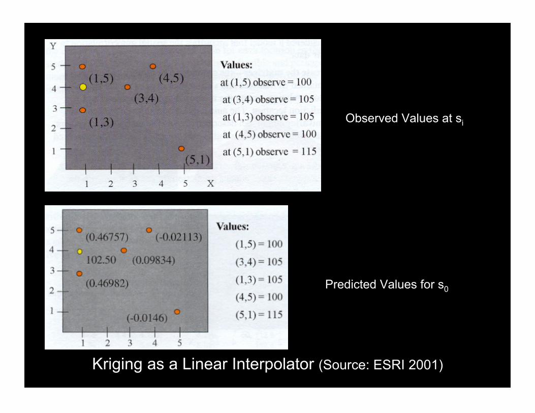
Observed Values at si

Kriging as a Linear Interpolator (Source: ESRI 2001)

Predicted Values for s0

© 2003 Luc Anselin, All Rights Reserved

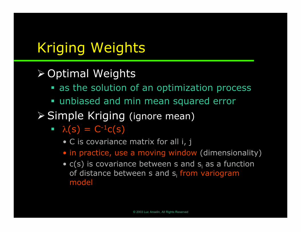
Kriging Weights

�Optimal Weights � as the solution of an optimization process � unbiased and min mean squared error

�Simple Kriging (ignore mean) � λ(s) = C-1c(s)

• C is covariance matrix for all i, j • in practice, use a moving window (dimensionality) • c(s) is covariance between s and si as a function

of distance between s and si from variogram model

© 2003 Luc Anselin, All Rights Reserved

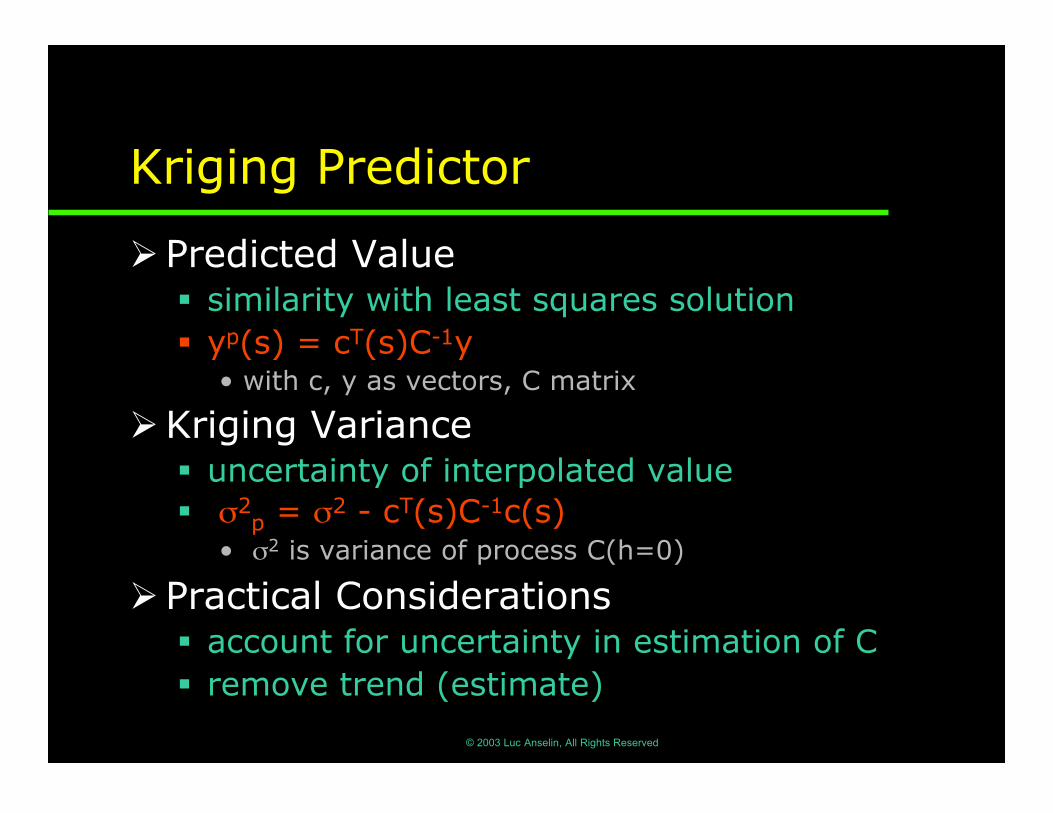
Kriging Predictor

�Predicted Value � similarity with least squares solution � yp(s) = cT(s)C-1y

• with c, y as vectors, C matrix

�Kriging Variance � uncertainty of interpolated value � σ2p = σ2 - cT(s)C-1c(s)

• σ2 is variance of process C(h=0)

�Practical Considerations � account for uncertainty in estimation of C � remove trend (estimate)

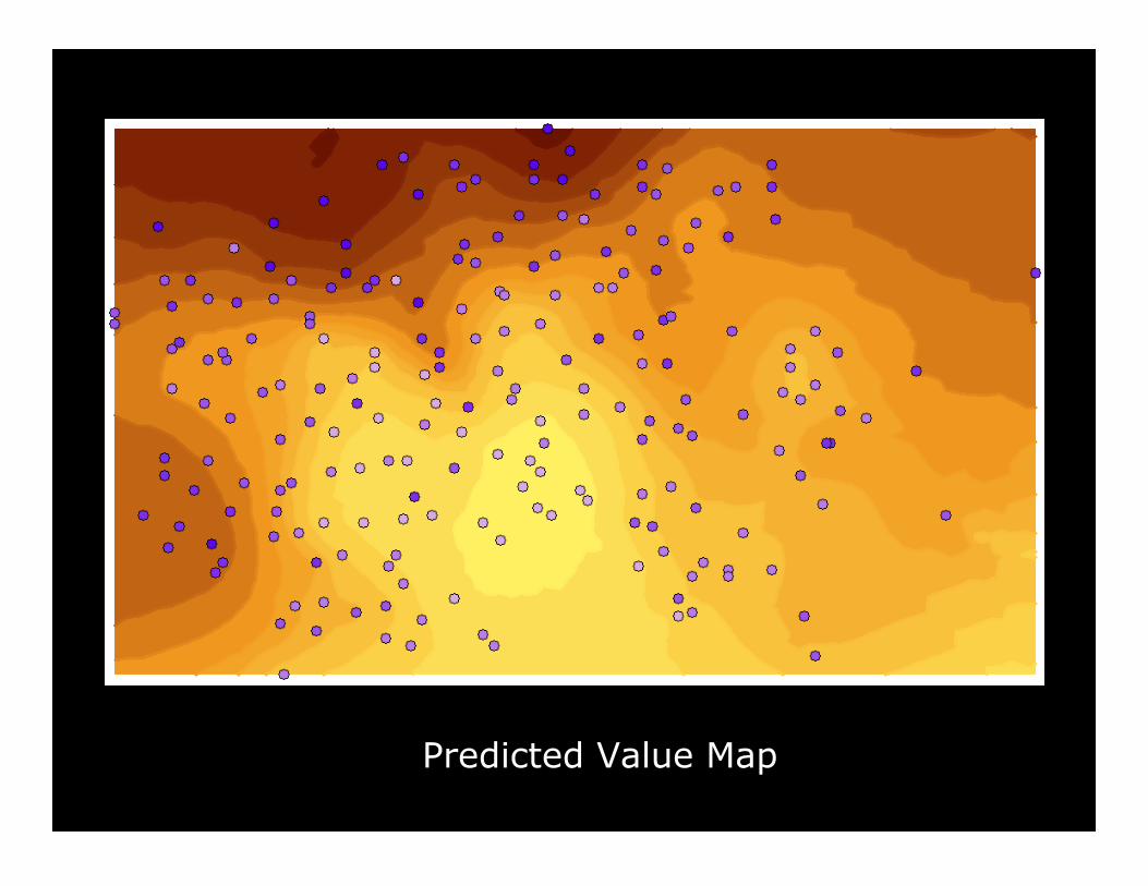
Predicted Value Map

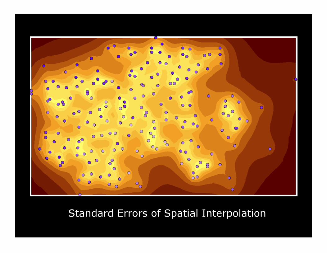
Standard Errors of Spatial Interpolation

© 2003 Luc Anselin, All Rights Reserved

Kriging Models

© 2003 Luc Anselin, All Rights Reserved

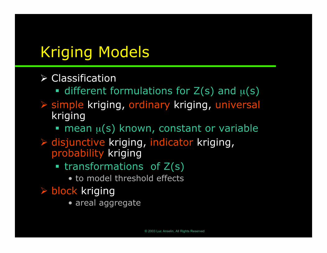
Kriging Models

� Classification � different formulations for Z(s) and µ(s)

� simple kriging, ordinary kriging, universal kriging � mean µ(s) known, constant or variable

� disjunctive kriging, indicator kriging, probability kriging � transformations of Z(s)

• to model threshold effects

� block kriging • areal aggregate

© 2003 Luc Anselin, All Rights Reserved

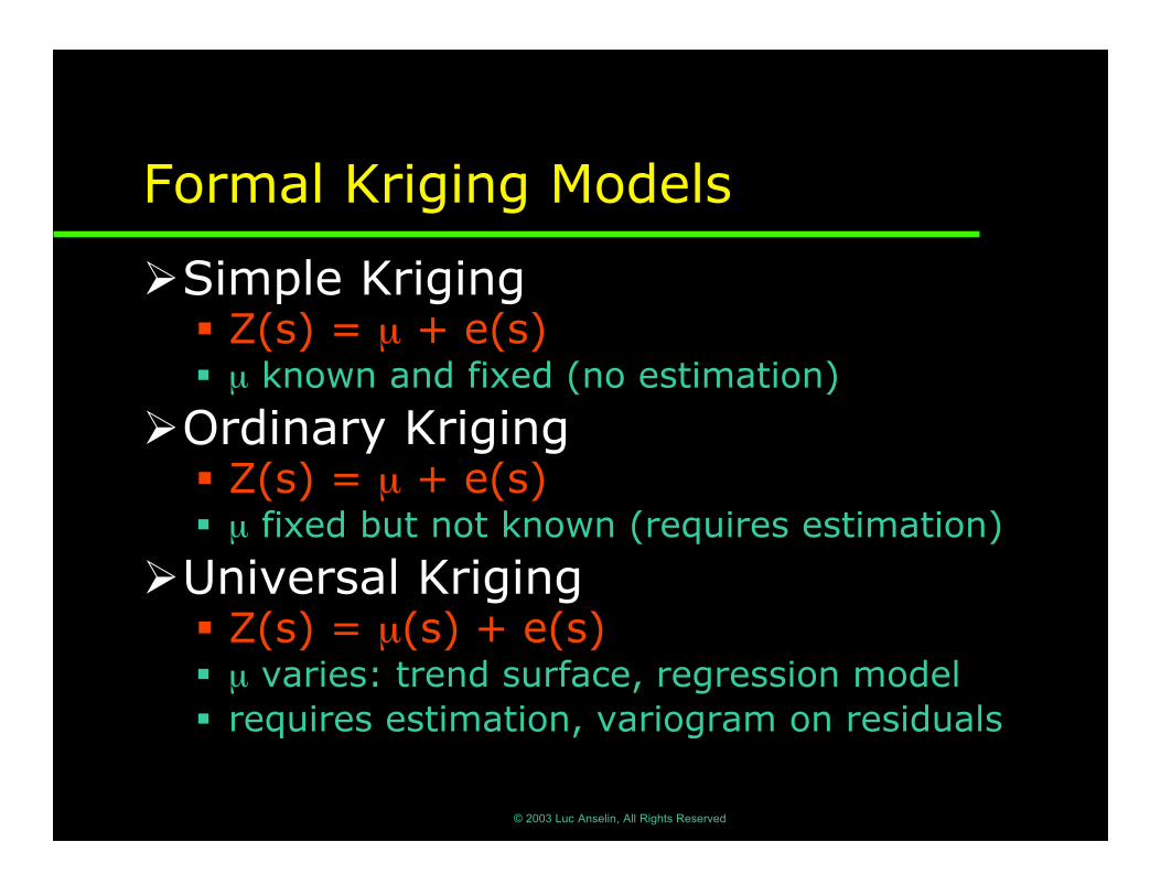
Formal Kriging Models

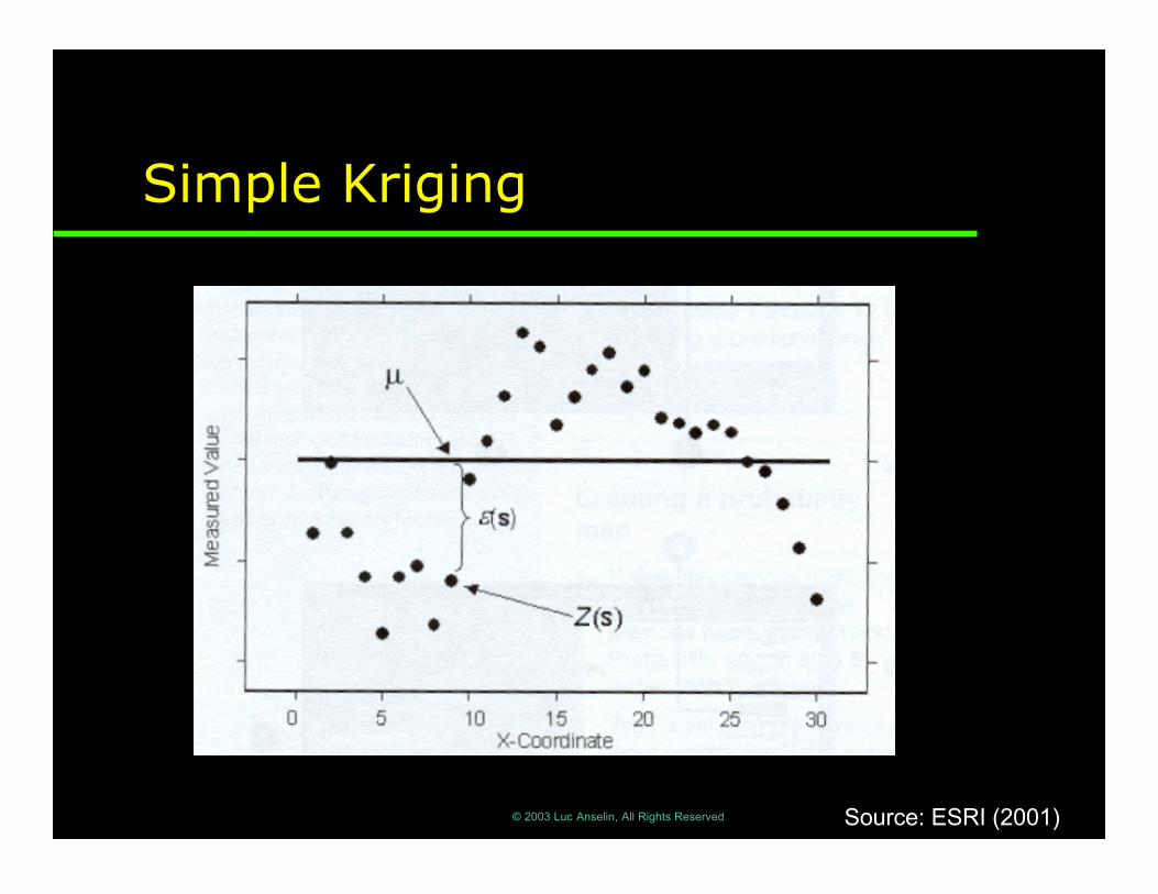
�Simple Kriging � Z(s) = µ + e(s) � µ known and fixed (no estimation)

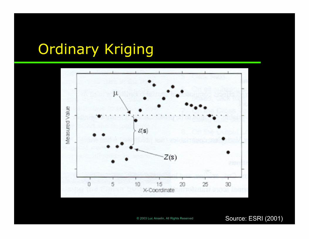
�Ordinary Kriging � Z(s) = µ + e(s) � µ fixed but not known (requires estimation)

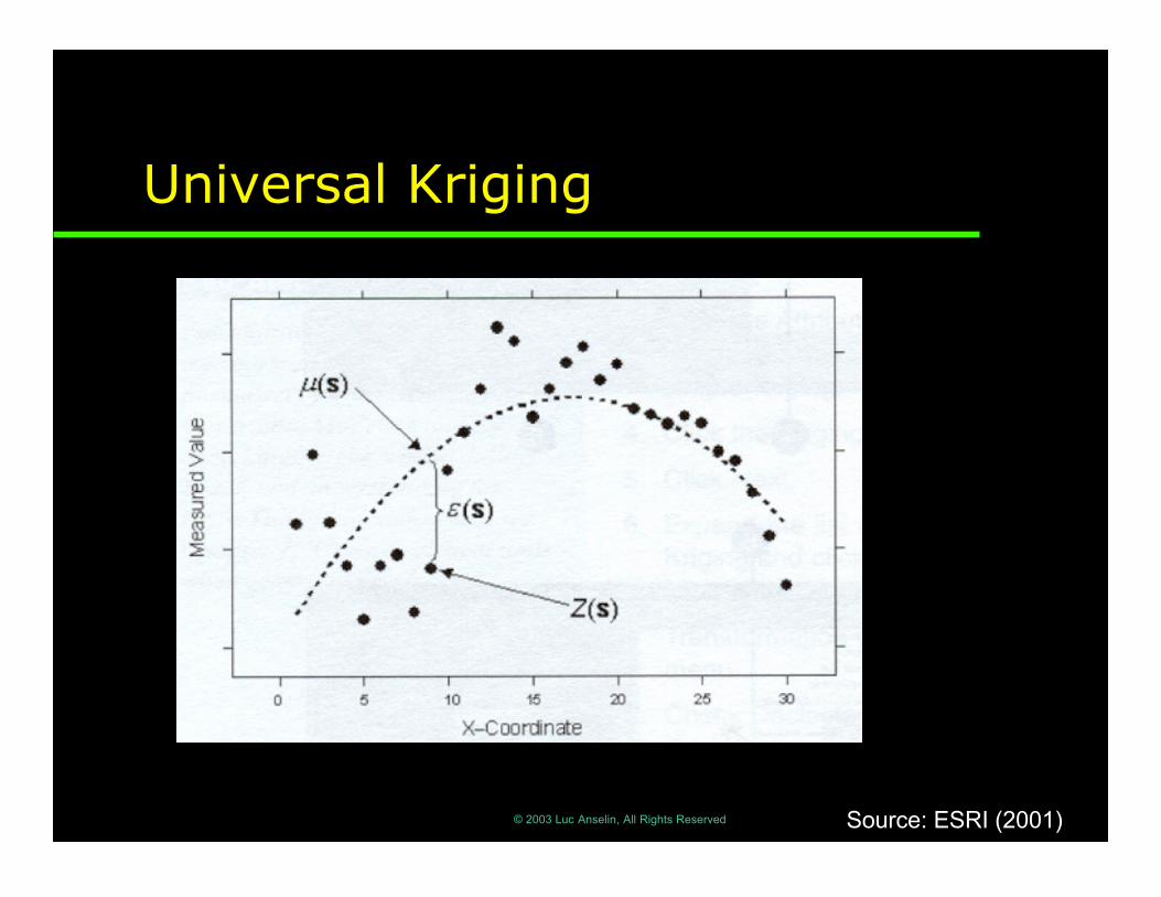
�Universal Kriging � Z(s) = µ(s) + e(s) � µ varies: trend surface, regression model � requires estimation, variogram on residuals

© 2003 Luc Anselin, All Rights Reserved

Simple Kriging

Source: ESRI (2001)

© 2003 Luc Anselin, All Rights Reserved

Ordinary Kriging

Source: ESRI (2001)

© 2003 Luc Anselin, All Rights Reserved

Universal Kriging

Source: ESRI (2001)

© 2003 Luc Anselin, All Rights Reserved

Spatial Interpolation by Kriging An Example

© 2003 Luc Anselin, All Rights Reserved

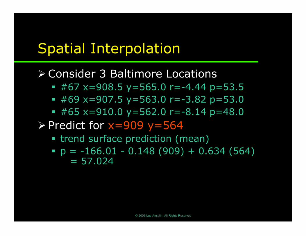
Spatial Interpolation

�Consider 3 Baltimore Locations � #67 x=908.5 y=565.0 r=-4.44 p=53.5 � #69 x=907.5 y=563.0 r=-3.82 p=53.0 � #65 x=910.0 y=562.0 r=-8.14 p=48.0

�Predict for x=909 y=564 � trend surface prediction (mean) � p = -166.01 - 0.148 (909) + 0.634 (564)

= 57.024

© 2003 Luc Anselin, All Rights Reserved

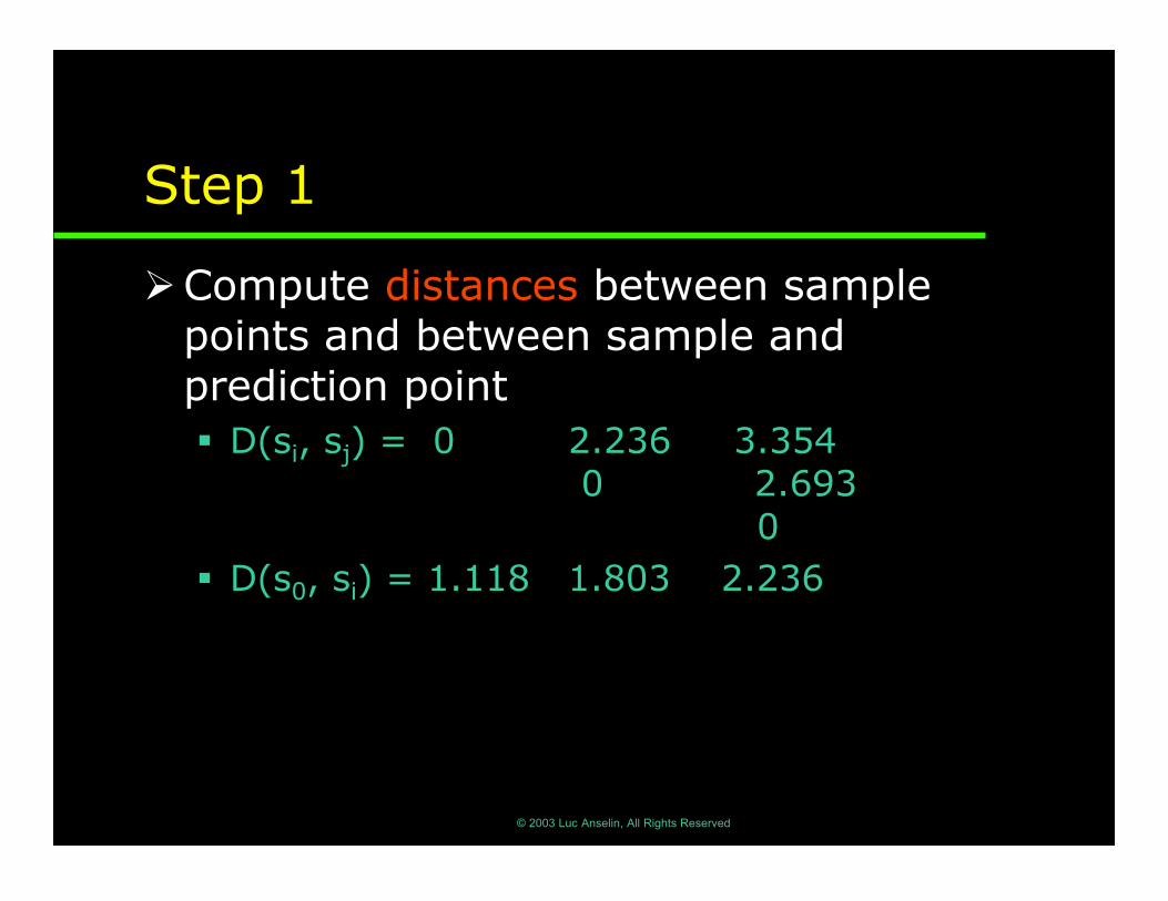
Step 1

�Compute distances between sample points and between sample and prediction point � D(si, sj) = 0 2.236 3.354

0 2.693 0

� D(s0, si) = 1.118 1.803 2.236

© 2003 Luc Anselin, All Rights Reserved

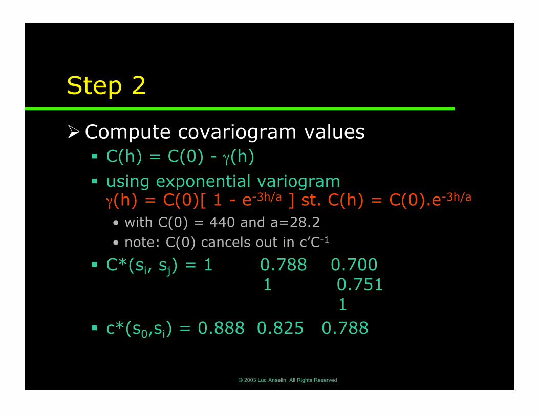
Step 2

�Compute covariogram values � C(h) = C(0) - γ(h)

� using exponential variogram γ(h) = C(0)[ 1 - e-3h/a ] st. C(h) = C(0).e-3h/a

• with C(0) = 440 and a=28.2 • note: C(0) cancels out in c’C-1

� C*(si, sj) = 1 0.788 0.700 1 0.751 1

� c*(s0,si) = 0.888 0.825 0.788

© 2003 Luc Anselin, All Rights Reserved

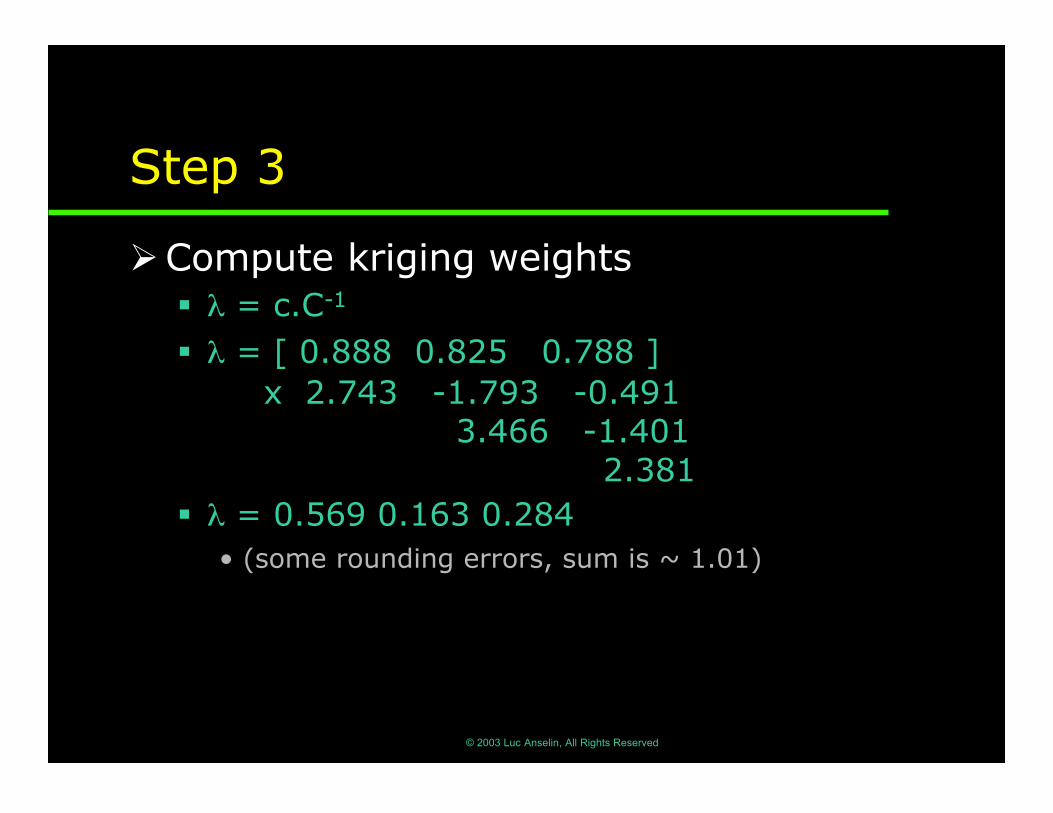
Step 3

�Compute kriging weights � λ = c.C-1

� λ = [ 0.888 0.825 0.788 ] x 2.743 -1.793 -0.491 3.466 -1.401 2.381

� λ = 0.569 0.163 0.284 • (some rounding errors, sum is ~ 1.01)

© 2003 Luc Anselin, All Rights Reserved

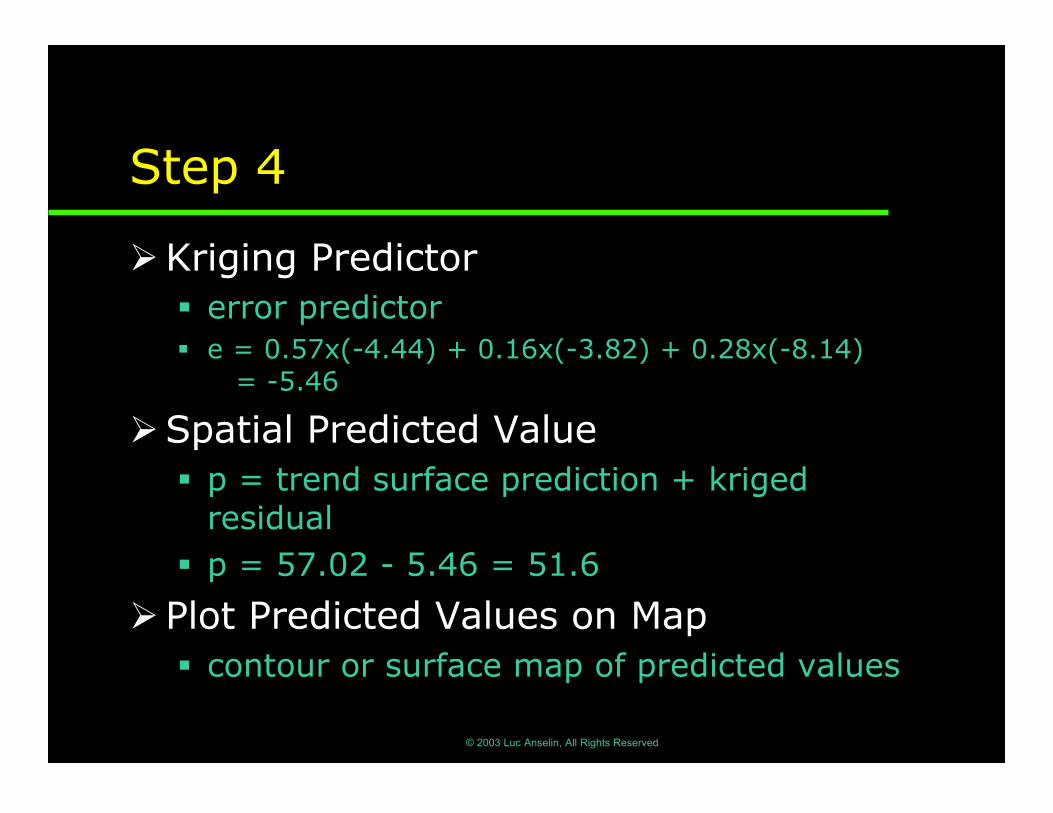
Step 4

�Kriging Predictor � error predictor � e = 0.57x(-4.44) + 0.16x(-3.82) + 0.28x(-8.14)

= -5.46

�Spatial Predicted Value � p = trend surface prediction + kriged

residual � p = 57.02 - 5.46 = 51.6

�Plot Predicted Values on Map � contour or surface map of predicted values

© 2003 Luc Anselin, All Rights Reserved

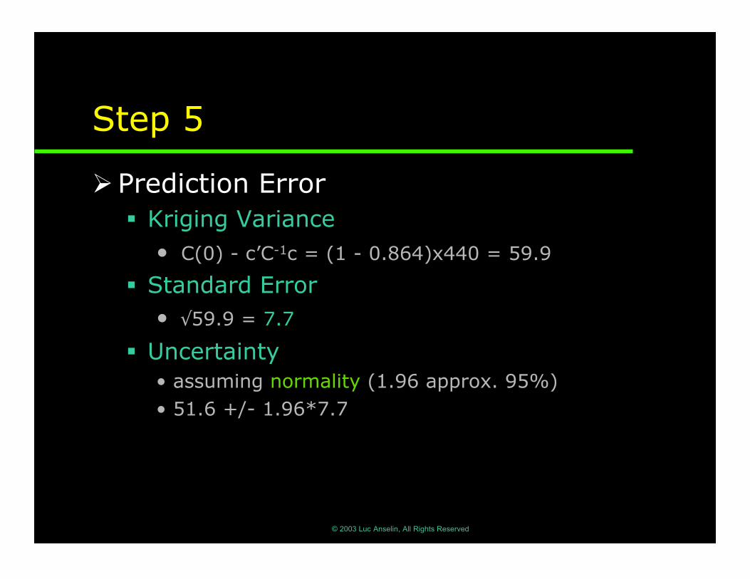
Step 5

�Prediction Error � Kriging Variance

• C(0) - c’C-1c = (1 - 0.864)x440 = 59.9 � Standard Error

• √59.9 = 7.7 � Uncertainty

• assuming normality (1.96 approx. 95%) • 51.6 +/- 1.96*7.7

© 2003 Luc Anselin, All Rights Reserved

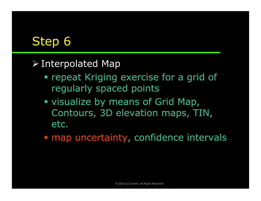
Step 6

� Interpolated Map � repeat Kriging exercise for a grid of

regularly spaced points � visualize by means of Grid Map,

Contours, 3D elevation maps, TIN, etc.

� map uncertainty, confidence intervals