Sparse Subspace Clustering via Diffusion Process

Qilin Li, Ling Li, Wanquan LiuCurtin University, Perth, Australia

kylinlovesummer@gmail.com

Abstract

Subspace clustering refers to the problem of cluster-ing high-dimensional data that lie in a union of low-dimensional subspaces. State-of-the-art subspace cluster-ing methods are based on the idea of expressing each datapoint as a linear combination of other data points while reg-ularizing the matrix of coefficients with `1, `2 or nuclearnorms for a sparse solution. `1 regularization is guaran-teed to give a subspace-preserving affinity (i.e., there are noconnections between points from different subspaces) un-der broad theoretical conditions, but the clusters may notbe fully connected. `2 and nuclear norm regularization of-ten improve connectivity, but give a subspace-preservingaffinity only for independent subspaces. Mixed `1, `2 andnuclear norm regularization could offer a balance betweenthe subspace-preserving and connectedness properties, butthis comes at the cost of increased computational complex-ity. This paper focuses on using `1 norm and alleviatingthe corresponding connectivity problem by a simple yet ef-ficient diffusion process on subspace affinity graphs. With-out adding any tuning parameter , our method can achievestate-of-the-art clustering performance on Hopkins 155 andExtended Yale B data sets.

1. IntroductionMany computer vision problems, such as image com-

pression [16], motion segmentation [26] and face clus-tering [15], deal with high-dimensional data. The high-dimensionality of the data not only increases the compu-tational time and memory requirements of algorithms, butalso decreases their performance due to the noise effect andinsufficient number of samples with respect to the ambi-ent space dimension, commonly referred to as the “curse ofdimensionality” [3]. However, even though data are high-dimensional, their intrinsic dimension is often much smallerthan the dimension of the ambient space, which has moti-vated the development of a number of techniques for find-ing a low-dimensional representation of a high-dimensionaldata set. Conventional techniques, such as Principal Com-

ponent Analysis (PCA), assume that the data is drawn froma single low-dimensional subspace of the high-dimensionalspace. In practice, however, such high-dimensional datausually lie close to multiple low-dimensional subspaces cor-responding to several classes or categories to which the databelong. In these scenarios, the task of clustering a high-dimensional data set into multiple classes becomes to thetask of assigning each data point to its own subspace andrecovering the underlying low-dimensional structure of thedata, a problem known in the literature as subspace cluster-ing [31].

In machine learning and computer vision communities,existing subspace clustering methods can be divided intofour main categories, including algebraic methods [6, 32],iterative methods [30, 21], statistical methods [22, 27],and spectral clustering-based methods [39, 14, 4, 10, 19].Among them, spectral-clustering based methods have be-come extremely popular due to their simplicity, theoreticalcorrectness, and empirical success. These methods gener-ally divide the problem into two steps: 1) Constructing anaffinity matrix based on certain model and 2) applying spec-tral clustering to the affinity matrix. In this paper, we fo-cus on the first step since the success of spectral clusteringhighly depends on having an appropriate affinity matrix.

State-of-the-art methods for constructing the affinity ma-trix in terms of subspace clustering are based on the self-expressiveness property of the data [9], i.e., each data pointin a union of subspaces can be efficiently reconstructedby a linear combination of all other data points: xj =∑i 6=j cijxi, where the coefficient cij is used to define the

affinity between points i and j as wij = |cij |+ |cji|. How-ever, this leads to an ill-posed problem with many possiblesolutions. To deal with this issue, the principle of sparsityis invoked. Specifically, every point is expressed as a sparselinear combination of all other data points by minimizingcertain norm of coefficient matrix. This problem can thenbe written as:

minC||C||, s.t. X = XC, diag(C) = 0, (1)

where X = [x1, ..., xN ] is the data matrix, C =

1

arX

iv:1

608.

0179

3v1

[cs

.CV

] 5

Aug

201

6

[C1, ..., CN ] is the coefficient matrix, || · || is a properly cho-sen regularizer.

The main difference among state-of-the-art methods liesin the choice of the regularizer. In Sparse Subspace Clus-tering (SSC) [9], the `1 norm is used for || · || as a con-vex relaxation of the `0 norm to promote the sparseness ofC. While under broad theoretical conditions [10, 38] thesparse representation produced by SSC is guaranteed to besubspace-preserving (i.e.,cij 6= 0 only if xi and xj are in thesame subspace), the affinity graph however may lack con-nectedness [] (i.e., data points from the same subspace maynot form a connected component of the affinity graph due tothe sparseness of the connections). In Low-Rank Represen-tation (LRR) [19] and Low-Rank Subspace Clustering [11],the nuclear norm || · ||∗ is adopted as a convex relaxation ofthe rank function. One benefit of nuclear norm is that thecoefficient matrix is generally dense, which alleviates theconnectivity issue of sparse representation based methods.However, the representation matrix is known to be subspacepreserving only when the subspaces are independent, whichsignificantly limits its applicability.

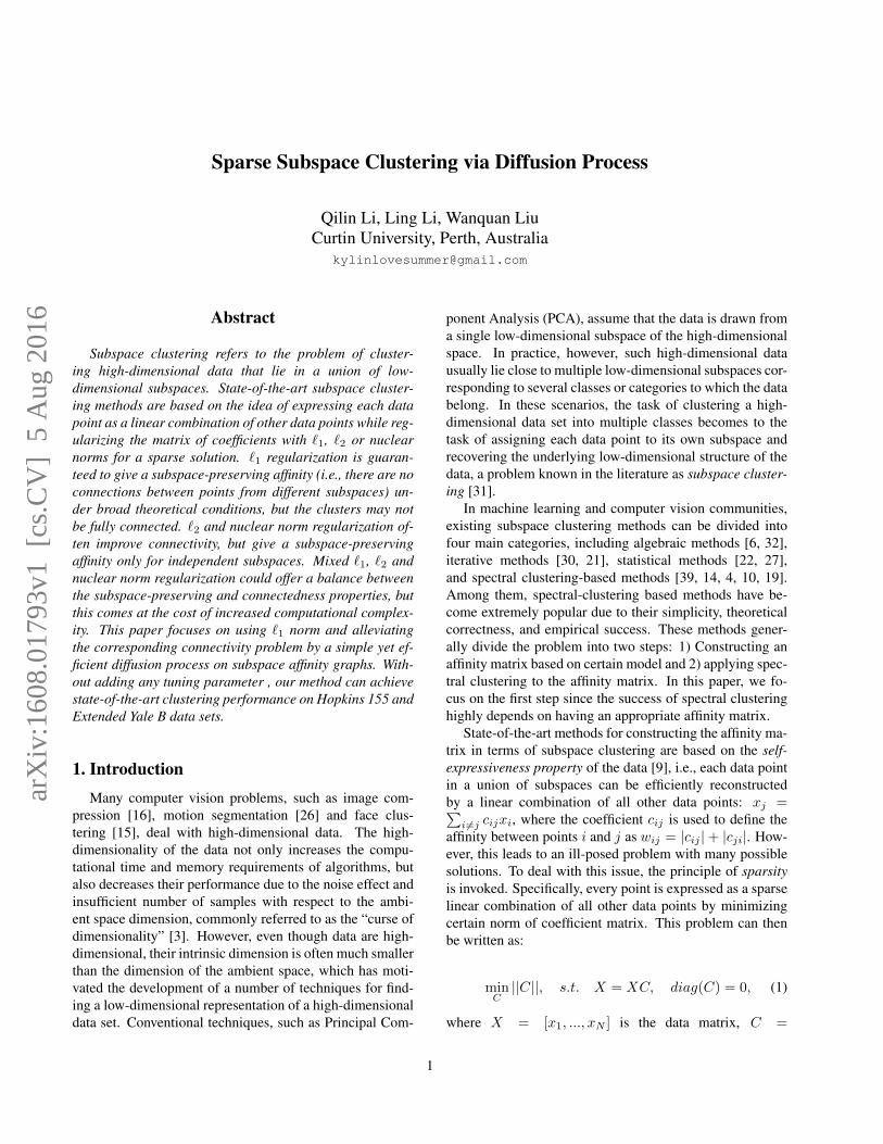
In this paper, we propose to use `1 norm for sparsityconstraint to best retain the subspace preserving property,and adopt a diffusion process on subspace of affinity graphto mitigate the connectedness problem. Specifically, thefist step is to learn a sparse affinity matrix by applying `1norm on optimization problem of (1). Diffusion process isthen adopted to spread the affinity values through the en-tire graph built upon the affinity matrix. Such a process isinterpretable as a random walk on the graph, where a so-called transition (affinity) matrix defines probabilities forwalking from one node to a neighboring node. One remark-able advantage here is, since the affinity matrix learned by`1 norm is subspace preserving, the random walk on thismatrix is guaranteed to be subspace constrained. There-fore, the connectivity within subspace is significantly en-hanced while the subspace preserving property remains un-altered. An illustrative example is given in Figure 1. Itclearly demonstrates that based on the sparse affinity matrixobtained by `1 norm, the proposed method could evidentlyimprove the affinity within subspaces while the sparsity be-tween subspaces is retained, yielding affinity matrix withexactly block-diagonal structure.

2. Related Work

2.1. Subspace clustering

State-of-the-art subspace clustering methods are basedon the self-expressiveness model. The main differenceamong those methods lies in the choice of the regularizeron the coefficient matrix. While different regularizers pos-sess their own advantages and drawbacks, [34, 25, 37] pro-pose to use mixed norms. For example, the low-rank sparse

subspace clustering (LRSSC) method [34] combines `1 andnuclear norm regularizer:

||C||∗ + λ||C||1, (2)

where λ controls the trade-off between the two regularizers.Likewise, [25, 37] propose to use a mixed `1 and `2 normgiven by

λ||C||1 +1− λ2||C||2, (3)

where λ plays a trade-off role between the two norms.These methods basically attempt to bridge the gap betweenthe subspace preserving and connectedness properties bythe trade-off of different norms.

[12] proposes to explicitly impose a block-diagonal con-straint by fixing the rank of Laplacian matrix. One benefit ofthis approach is that it can be applied to all the affinity con-struction methods straightforwardly. The Structured SparseSubspace Clustering (SSSC) [18] integrates the two stages,affinity learning and spectral clustering, into one unified op-timization framework. Their observation is that the cluster-ing results can help the self-expressiveness model to yield abetter affinity matrix.

2.2. Diffusion processes

Diffusion process is widely used in the field of retrieval[35, 1, 8, 33, 7], in which the task is retrieving the most sim-ilar instances to a provided query element from a potentiallylarge database. Conventional approaches are usually basedon analyzing pairwise affinity/distance values which are di-rectly used to rank the most similar elements afterwards.Such approaches has the main limitation that the structureof the underlying data manifold is completely ignored. Forthis reason, instead of considering pairwise affinity individ-ually, diffusion process is adopted to derive context sensi-tive measures, and it has shown to be an indispensable toolfor improving retrieval performance [7].

Diffusion process is generally start with a affinity matrixAN×N . The first step is to interpret the matrix A as a undi-rected graph G = (V,E), consisting of N nodes vi ∈ V ,and edges eij ∈ E that link nodes to each other. The edgeweights are fixed to the affinity values Aij . Diffusion pro-cess then spreads the affinity values through the entire graphbased on the defined edge weights.

Diffusion process can be interpreted as a Markov randomwalk on a graph G = (V,E). To this end, we first definethe transition matrix of random walk as

P = D−1A, (4)

where D is a diagonal matrix with Dii =∑nk=1A(i, k).

Obviously, P is a row-stochastic matrix, containing thetransition probabilities for a random walk in the correspond-ing graph. With a simple undate rule At+1 = AtP , the

2

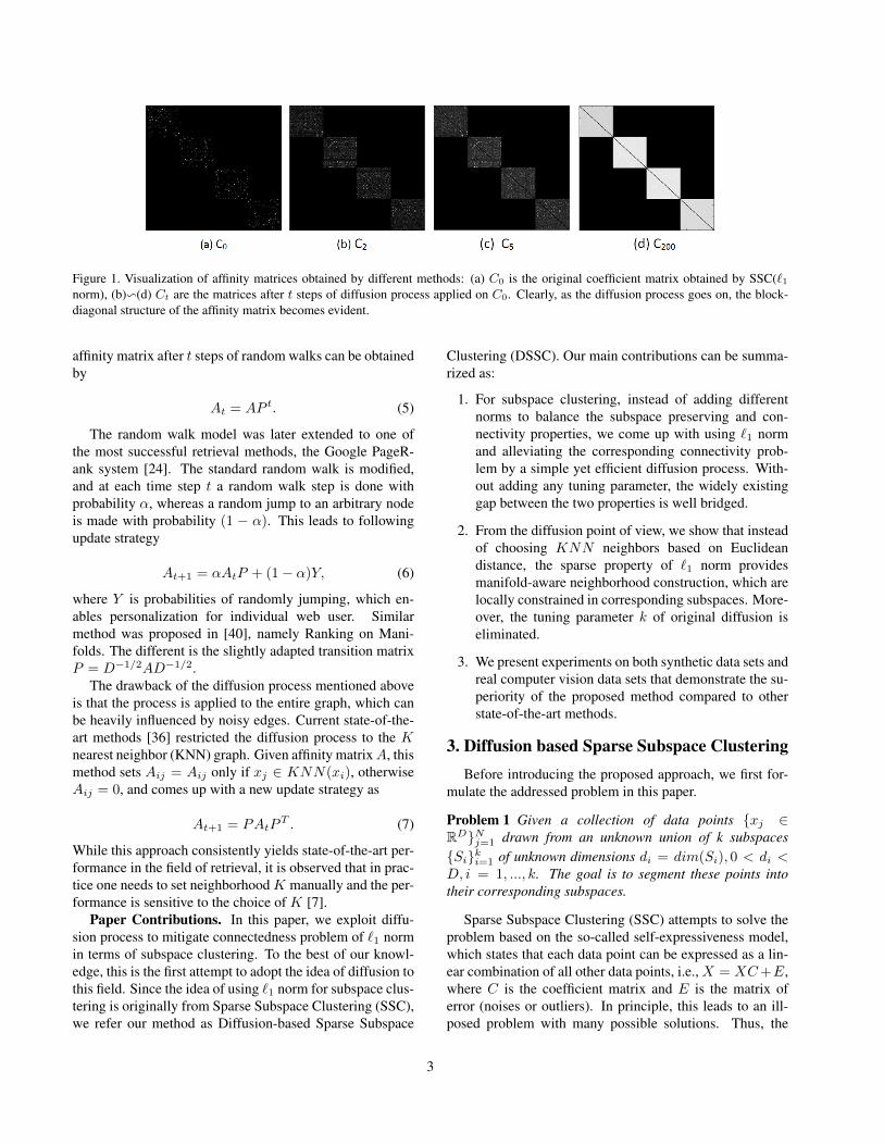
Figure 1. Visualization of affinity matrices obtained by different methods: (a) C0 is the original coefficient matrix obtained by SSC(`1norm), (b)v(d) Ct are the matrices after t steps of diffusion process applied on C0. Clearly, as the diffusion process goes on, the block-diagonal structure of the affinity matrix becomes evident.

affinity matrix after t steps of random walks can be obtainedby

At = AP t. (5)

The random walk model was later extended to one ofthe most successful retrieval methods, the Google PageR-ank system [24]. The standard random walk is modified,and at each time step t a random walk step is done withprobability α, whereas a random jump to an arbitrary nodeis made with probability (1 − α). This leads to followingupdate strategy

At+1 = αAtP + (1− α)Y, (6)

where Y is probabilities of randomly jumping, which en-ables personalization for individual web user. Similarmethod was proposed in [40], namely Ranking on Mani-folds. The different is the slightly adapted transition matrixP = D−1/2AD−1/2.

The drawback of the diffusion process mentioned aboveis that the process is applied to the entire graph, which canbe heavily influenced by noisy edges. Current state-of-the-art methods [36] restricted the diffusion process to the Knearest neighbor (KNN) graph. Given affinity matrixA, thismethod sets Aij = Aij only if xj ∈ KNN(xi), otherwiseAij = 0, and comes up with a new update strategy as

At+1 = PAtPT . (7)

While this approach consistently yields state-of-the-art per-formance in the field of retrieval, it is observed that in prac-tice one needs to set neighborhoodK manually and the per-formance is sensitive to the choice of K [7].

Paper Contributions. In this paper, we exploit diffu-sion process to mitigate connectedness problem of `1 normin terms of subspace clustering. To the best of our knowl-edge, this is the first attempt to adopt the idea of diffusion tothis field. Since the idea of using `1 norm for subspace clus-tering is originally from Sparse Subspace Clustering (SSC),we refer our method as Diffusion-based Sparse Subspace

Clustering (DSSC). Our main contributions can be summa-rized as:

1. For subspace clustering, instead of adding differentnorms to balance the subspace preserving and con-nectivity properties, we come up with using `1 normand alleviating the corresponding connectivity prob-lem by a simple yet efficient diffusion process. With-out adding any tuning parameter, the widely existinggap between the two properties is well bridged.

2. From the diffusion point of view, we show that insteadof choosing KNN neighbors based on Euclideandistance, the sparse property of `1 norm providesmanifold-aware neighborhood construction, which arelocally constrained in corresponding subspaces. More-over, the tuning parameter k of original diffusion iseliminated.

3. We present experiments on both synthetic data sets andreal computer vision data sets that demonstrate the su-periority of the proposed method compared to otherstate-of-the-art methods.

3. Diffusion based Sparse Subspace ClusteringBefore introducing the proposed approach, we first for-

mulate the addressed problem in this paper.

Problem 1 Given a collection of data points {xj ∈RD}Nj=1 drawn from an unknown union of k subspaces{Si}ki=1 of unknown dimensions di = dim(Si), 0 < di <D, i = 1, ..., k. The goal is to segment these points intotheir corresponding subspaces.

Sparse Subspace Clustering (SSC) attempts to solve theproblem based on the so-called self-expressiveness model,which states that each data point can be expressed as a lin-ear combination of all other data points, i.e., X = XC+E,where C is the coefficient matrix and E is the matrix oferror (noises or outliers). In principle, this leads to an ill-posed problem with many possible solutions. Thus, the

3

sparsity constraint is invoked by `1 minimization, leadingto the following optimization problem

minC||C||1+ ||E||` s.t. X = XC+E, diag(C) = 0,

(8)where the Frobenius norm or `1 norm is used for || · ||` tohandle noise or outliers. The SSC algorithm proceeds bysolving the optimization problem in (8) using the ADMMmethod. The optimal coefficient C is then used to define anaffinity matrix |C|+ |CT |. The segmentation of the data isfinally obtained by applying spectral clustering to the nor-malized Laplacian.

While SSC works well in practice, one possible draw-back is `1 finds the sparse representation of each data pointindividually. In the case of clean data, SSC is guaran-teed to be subspace-preserving, i.e., there are no connec-tions between points from different subspaces. However,the within-subspace connections are usually sparse, i.e., Cijcould be zero even xi and xj are in the same subspace. It isnot a problem as long as the connections are still subspace-preserving. But in the case of noisy data, there is no theo-retical guarantee that the nonzero coefficients correspond topoints in the same subspace. Imaging there are connectionsbetween points from different subspaces, spectral clusteringcannot be able to appropriately cut the graph, as shown inFigure 3.

Diffusion process is capable to deal with this issue by ex-ploiting the contextual affinities. Given the affinity matrixW = |C| + |CT |, where C is obtained by solving (8), dif-fusion process is encoded into computing the power of theaffinity matrix, which is

Wt =W t, (9)

where t corresponds t steps of diffusion process. Obviously,such a process is sensitive to the step t. In order to makethe diffusion process independent from t, we consider theaccumulation of all t. Thus, the diffusion process is

Wt =

t∑i=0

W i. (10)

We assume that W is nonnegative and the sum of eachrow is smaller than one. A matrix W that satisfies theserequirements can be easily constructed from a stochasticmatrix. Note that the absolute values of the eigenvaluesis bounded by the maximum of the rowwise sums. There-fore, the maximum of the absolute values of the eigenval-ues ofW is smaller than one. Consequently, (10) convergesto a fixed and nontrivial solution given by limt→∞Wt =(I −W )−1, where I is the identity matrix.

To further incorporate the contextual affinity, it is shownin [36] that the diffusion process on higher order tensor

product graph is promising for revealing the intrinsic re-lation between data points. Given graph G = (V,E)constructed from affinity matrix W , the tensor productgraph is defined as the Kronecker product of original graph,G = G

⊗G. The corresponding affinity matrix is W =

W⊗W . In particular, we have

W(α, β, i, j) =W (α, β) ·W (i, j) = wα,β · wi.j . (11)

Thus, if W ∈ Rn×n, then W =W⊗W ∈ Rnn×nn.

The diffusion process is then defined on the higher ordertensor as

Wt =

t∑i=0

Wi. (12)

Since the sum of each row of W is smaller than 1, wehave

∑βj

W(α, β, i, j) =∑βj

wαβwij =∑β

wαβ∑j

wij < 1.

(13)As is the case for (10), the process (12) also converges to

a fixed and nontrivial solution,

limt→∞

Wt = limt→∞

t∑i=0

Wi = (I −W)−1 (14)

Since our goal is to learn a new affinity matrix W ∗ ofsize n× n, it is defined as

W ∗ = vec−1((I −W)−1vec(I)), (15)

where I is the identity matrix and vec is an operator thatstacks the columns of a matrix one after the next into a col-umn vector. The inverse of vec is denoted as vec−1.

While the tensor graph provides adequate underlyingstructure of the data, it is impractical for large scale prob-lems due to the demand of high storage and computing cost.Therefore, we use an iterative algorithm for the diffusionprocess on tensor graph. First, we define A1 = W and theupdate strategy as

At+1 =WAtWT + I, (16)

where I is the identity matrix. The diffusion process be-comes the iteration of (16) until convergence. To prove theconvergence of (16), we first transform (16) to

4

At+1 =WAtWT + I =W (WAt−1W

T + I)WT + I

=W 2At−1(WT )2 +WIWT + I = ...

=W tW (WT )t +W t−1I(WT )t−1 + ...+ I

=W tW (WT )t +

t−1∑i=0

W iI(WT )i. (17)

Since we assume the sum of each row of W < 1, wehave limt→∞W tW (WT )t = 0, consequently,

limt→∞

At+1 = limt→∞

t−1∑i=0

W iI(WT )i. (18)

As shown in [36], it can be proven by induction that

limt→∞

t−1∑i=0

W iI(WT )i = vec−1((I −W)−1vec(I)). (19)

So we have

limt→∞

At+1 = vec−1((I −W)−1vec(I)). (20)

Hence, the iterative algorithm (16) yields the same affinitiesas the diffusion process on tensor graph.

3.1. A graph view of the diffusion process

With `1 minimization, SSC seeks sparse representationfor each data point individually. The corresponding affin-ity graph reveals the pairwise affinity as the “shortest path”between them, which is susceptible to noise. The proposedDSSC derives the affinity by considering the “volume ofpaths” through a diffusion process. One remarkable inven-tion is, with `1 norm, the “volume of paths” are restricted insubspaces, resulting in the enhancement of within-subspaceaffinity and constant of between-subspace affinity.

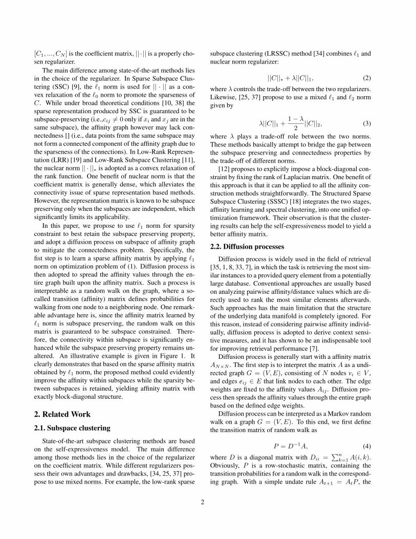
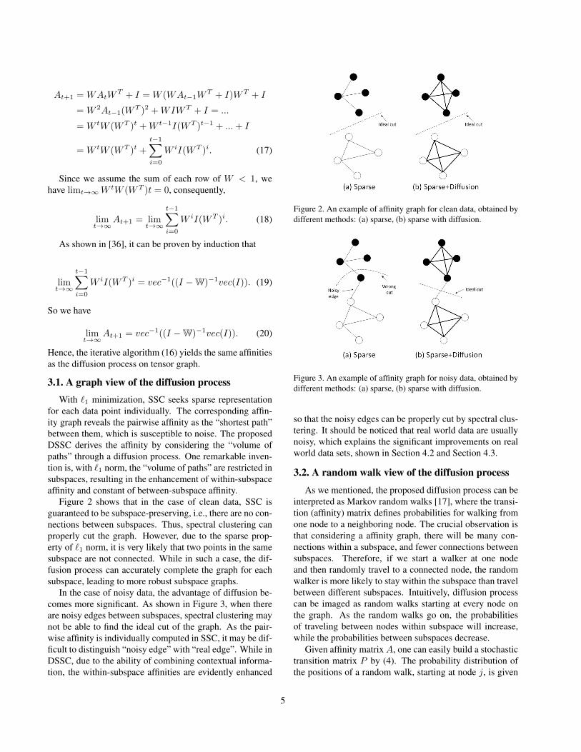
Figure 2 shows that in the case of clean data, SSC isguaranteed to be subspace-preserving, i.e., there are no con-nections between subspaces. Thus, spectral clustering canproperly cut the graph. However, due to the sparse prop-erty of `1 norm, it is very likely that two points in the samesubspace are not connected. While in such a case, the dif-fusion process can accurately complete the graph for eachsubspace, leading to more robust subspace graphs.

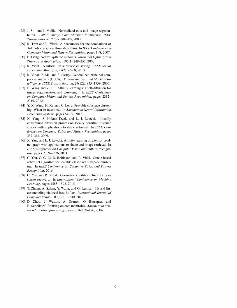
In the case of noisy data, the advantage of diffusion be-comes more significant. As shown in Figure 3, when thereare noisy edges between subspaces, spectral clustering maynot be able to find the ideal cut of the graph. As the pair-wise affinity is individually computed in SSC, it may be dif-ficult to distinguish “noisy edge” with “real edge”. While inDSSC, due to the ability of combining contextual informa-tion, the within-subspace affinities are evidently enhanced

Figure 2. An example of affinity graph for clean data, obtained bydifferent methods: (a) sparse, (b) sparse with diffusion.

Figure 3. An example of affinity graph for noisy data, obtained bydifferent methods: (a) sparse, (b) sparse with diffusion.

so that the noisy edges can be properly cut by spectral clus-tering. It should be noticed that real world data are usuallynoisy, which explains the significant improvements on realworld data sets, shown in Section 4.2 and Section 4.3.

3.2. A random walk view of the diffusion process

As we mentioned, the proposed diffusion process can beinterpreted as Markov random walks [17], where the transi-tion (affinity) matrix defines probabilities for walking fromone node to a neighboring node. The crucial observation isthat considering a affinity graph, there will be many con-nections within a subspace, and fewer connections betweensubspaces. Therefore, if we start a walker at one nodeand then randomly travel to a connected node, the randomwalker is more likely to stay within the subspace than travelbetween different subspaces. Intuitively, diffusion processcan be imaged as random walks starting at every node onthe graph. As the random walks go on, the probabilitiesof traveling between nodes within subspace will increase,while the probabilities between subspaces decrease.

Given affinity matrix A, one can easily build a stochastictransition matrix P by (4). The probability distribution ofthe positions of a random walk, starting at node j, is given

5

by the j-th row of the transition matrix. After t time steps,the probability of a random walk starting at node j at time0, to be at node i at time t is thus,

pt(i|j) = P ti,j . (21)

Under mild conditions [5], we obtain in this way an ergodicMarkov process with a single stationary distribution π =(π1, ..., πn), where πi = di/vol(V ), di is the degree ofnode i, V is the set of all nodes. It is easy to verify thatthis distribution is a right-eigenvector of the t-step transitionmatrix (for every t), e.g. PTπ = π, since πi =

∑Pi,jπj .

As we know, there is a tight relation between randomwalks and spectral segmentation [23]. We take the Normal-ized Cut [28] (NCut) as an example of spectral segmenta-tion. The goal of NCut algorithm is to segment an imageinto two disjoint parts by minimizing

NCut(A,A) =

(1

vol(A)+

1

vol(A)

) ∑i∈A,j∈A

Aij . (22)

As derived by [23], the objective function of NCut (27) canbe expressed in the framework of random walk as follows.For two disjoint subsets A, B ⊂ V , assume we run a ran-dom walk starting with X0 in the stationary distribution π.We define

P (B|A) = P (X1 ∈ B|X0 ∈ A) (23)

as the probability of the random walk transition from set Ato set B. First of all it can be observed that

P (X0 ∈ A,X1 ∈ B) =∑

i∈A,j∈BP (Xi, Xj)

=∑

i∈A,j∈Bπipij

=∑

i∈A,j∈B

divol(V )

aijdi

=1

vol(V )

∑i∈A,j∈B

aij . (24)

With the Bayes’ Rules, we have the posterior probability

P (B|A) = P (X0 ∈ A,X1 ∈ B)

P (X0 ∈ A

=

(1

vol(V )

∑i∈A,j∈B

aij

)(vol(A)

vol(V )

)−1=

1

vol(A)

∑i∈A,j∈B

aij . (25)

Follow this, the definition of NCut can be written as

NCut(A,A) = P (A|A) + P (A|A). (26)

While originally the objective of NCut algorithm is to findthose regions that the between connections are minimized,it can be interpreted as to find regions in which the probabil-ities of random walkers escape from these regions are low,with the theory of random walk.

Denoting the transition matrix after t time steps ran-dom walk as Pt, we know that Pt(A|A) < P (A|A) whilePt(A|A) > P (A|A). Let NCut∗ be the NCut criterionon the transition matrix after random walk, the followingholds,

NCut∗(A,A) = Pt(A|A) + Pt(A|A) < NCut(A,A),(27)

which explains why random walk (diffusion process) canimprove the performance of spectral segmentation.

4. ExperimentsExperiments are demonstrated in this section. We evalu-

ate the proposed DSSC approach on a synthetic data set, amotion segmentation data set, and a face clustering data setto validate its effectiveness.

Experimental Setup. Since the proposed DSSC is builtupon the standard SSC [10], we keep all settings in DSSCthe same as in SSC. As for diffusion process, since it isguaranteed to converge, we set the iteration to 200 for allexperiments. The performance is validated by clusteringerror, which is measured by

clustering error =# of missclassified points

total # of points.

(28)

4.1. Experiments on synthetic data

Data Generation. We construct 5 subspaces {S}5i=1 ⊂R100 whose bases {Ui}5i=1 are obtained by Ui = TiU, 1 ≤i ≤ 5, where U is a random matrix of dimension 100×5 and T 100×100

i is a random rotation. We sample 50 datapoints from each subspace byXi = UiQi, where the entriesof Qi ∈ R5,50 are i.i.d. samples from a standard Gaussian.Some data vectors x are then randomly chosen to corrupt byGaussian noise with zero mean and variance 0.3||x||.

Experimental results are presented in Table 1. It can beobserved that the proposed DSSC consistently outperformsSSC. In the case of clean data (no corruptions), both SSCand DSSC achieve perfect clustering with error rates equalto 0. As the corruptions increase, so do the chance of addingnoise edges into the corresponding affinity graph. In thiscase, spectral clustering cannot find the appropriate cut of

6

Table 1. Clustering Errors on Synthetic Dataset.

Corruptions 0 10% 20% 30% 40% 50% 60% 70% 80% 90% 100%SSC 0 2.88 6.90 13.26 18.66 24.62 30.16 34.42 38.80 40.20 43.00

DSSC 0 1.60 4.80 9.74 14.40 17.64 22.80 28.98 32.80 36.00 39.74

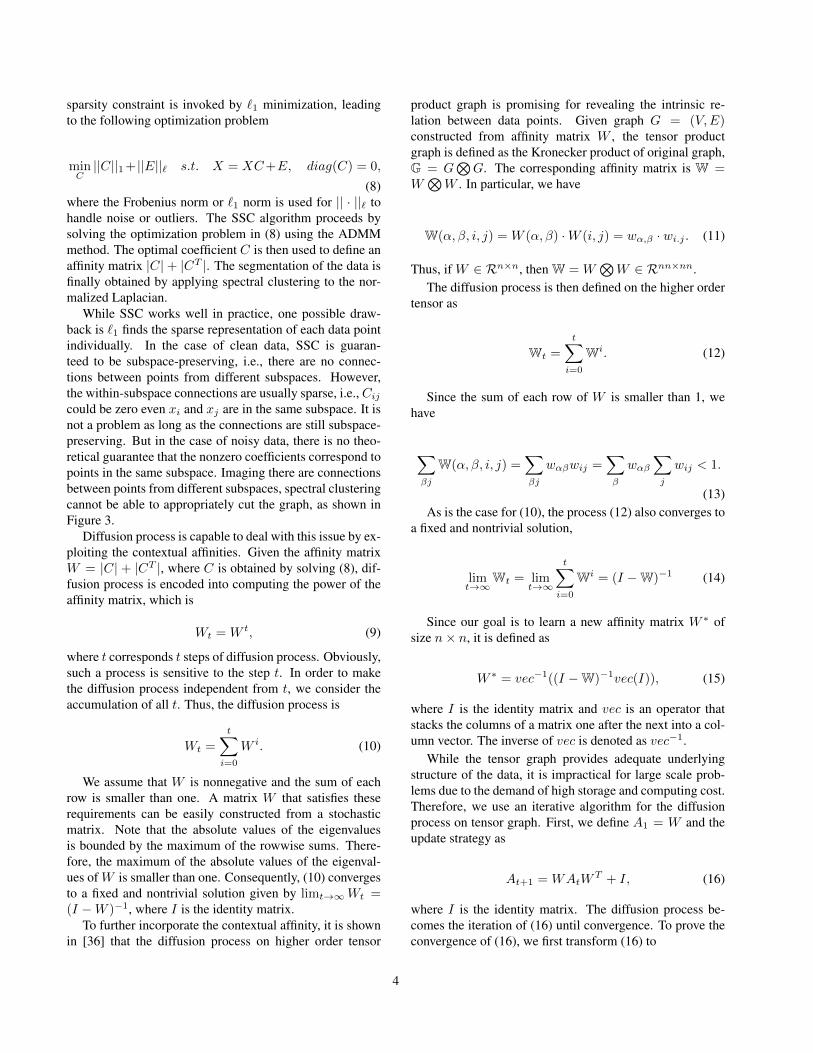
Figure 4. Example frames from videos in the Hopkins 155 [29].

the graph in SSC. While in DSSC, those noisy edges arewell detected due to the within subspaces edges are signif-icantly enhanced by the diffusion process, as demonstratedin Figure 2 and Figure 3.

4.2. Experiments on Motion Segmentation

Motion segmentation refers to the problem of segment-ing a video sequence of multiple rigidly moving objects intomultiple spatiotemporal regions that correspond to differentmotions in the scene (see Figure 4). This problem is of-ten solved by extracting and tracking a set of feature pointsthrough all frames of the video. Each data point, whichis also called a feature trajectory, corresponds to a vectorobtained by stacking all feature points. Under the affineprojection model, all feature trajectories associated with asingle rigid motion lie in an affine subspace of dimensionat most 3 [10]. Therefore, motion segmentation reduces toclustering of these trajectories in a union of subspaces.

We evaluate the proposed DSSC algorithm with otherstate-of-the-art subspace clustering methods, i.e., SSC [10],SSSC [18], LRR [19], LSR [20], BDSSC [12], LRSC [11],on the Hopkins 155 motion segmentation data set [29] forthe multi-view affine motion segmentation. It consists of155 video sequences, where 120 of the videos have two mo-tions and 35 of the videos have three motions. We evaluateaverage performance on three cases: 2 motions, 3 motions,and all. Experimental results are presented in Table 2. Theresult for LRSC is cited from [11], while the others are citedfrom [18]. Note that the proposed DSSC achieves the bestperformances on all cases.

4.3. Experiments on Face Clustering

Given face images of multiple subjects acquired with afixed pose and varying illumination, we consider the prob-lem of clustering images according to their subjects. It hasbeen shown that, under the Lambertian assumption, imagesof a subject with a fixed pose and varying illumination lieclose to a linear subspace of dimension 9 [2]. Thus, faceclustering can be also considered as a subspace clustering

problem, where each subject lies in a 9D subspace.We evaluate the clustering performance of the proposed

DSSC as well as other state-of-the-art methods on the Ex-tended Yale B data set [13]. It contains 2,414 frontal faceimages of 38 subjects, with 64 images per subject acquiredunder different illumination conditions. In our experiments,we follow the same settings introduced in [10]. It should benoticed that the Extended Yale B data set is more challeng-ing for subspace segmentation than the Hopkins 155 data setdue to the heave noise, high-dimensional space, and largenumber of subspace in the data.

Experimental results are presented in Table 3. The re-sults are directly cited from [18], which is a fair compari-son as we use exactly same experimental settings. It can beobserved that the proposed DSSC performs the best resultson all cases. Note that on this more challenging data set,DSSC achieves significant improvements compared to thestate-of-the-art methods. It is worth mentioning that thesesignificant improvements are achieved by a parameter-freediffusion process, while other methods usually add in tun-ing parameters for flexibility.

5. ConclusionIn this work, we investigated diffusion process for sparse

subspace clustering and proposed a new subspace cluster-ing method, namely DSSC. Specifically, after we obtainedaffinity matrix by `1 minimization, we adopted a diffusionprocess to spread the affinity value. With the subspace-preserving property of `1 norm, such a diffusion processis remarkably constrained within each subspaces, yieldingenhanced within-subspace affinity and unaltered between-subspace affinity. Moreover, we explained the diffusionprocess in the views of graph and random walk, and gavetheoretical justifications on how does the diffusion processimprove the performance of spectral clustering. Exten-sive experiments verified that our proposed diffusion basedsparse subspace clustering method, without adding in tun-ing parameter, could significantly improve the state-of-the-art performance.

References[1] X. Bai, X. Yang, L. J. Latecki, W. Liu, and Z. Tu. Learn-

ing context-sensitive shape similarity by graph transduction.Pattern Analysis and Machine Intelligence, IEEE Transac-tions on, 32(5):861–874, 2010.

[2] R. Basri and D. W. Jacobs. Lambertian reflectance and linearsubspaces. Pattern Analysis and Machine Intelligence, IEEETransactions on, 25(2):218–233, 2003.

7

Table 2. Motion Segmentation Errors(%) on Hopkins 155 Dataset.

Methods LRR [19] LRSC [11] LSR [20] BDSSC [12] SSC [10] SSSC[18] DSSC2 motions 3.76 3.69 2.20 2.29 1.95 1.94 1.683 motions 9.92 7.69 7.13 4.95 4.94 4.92 4.64

All 5.15 4.59 3.31 2.89 2.63 2.61 2.35

Table 3. Clustering Errors (%) on the Extended Yale B Dataset.

Methods LRR [19] LRSC [11] LSR [20] BDSSC [12] SSC [10] SSSC[18] DSSC2 subjects 6.74 3.15 6.72 3.90 1.87 1.27 0.613 subjects 9.30 4.71 9.25 17.70 3.35 2.71 1.255 subjects 13.94 13.06 13.87 27.50 4.32 3.41 2.808 subjects 25.61 21.25 25.98 33.20 5.99 4.15 4.04

10 subjects 29.53 29.58 28.33 39.53 7.29 5.16 4.84

[3] R. E. Bellman. Dynamic Programming. Princeton Univ.Press, 1957.

[4] G. Chen and G. Lerman. Spectral curvature cluster-ing (SCC). International Journal of Computer Vision,81(3):317–330, 2009.

[5] F. R. Chung. Spectral graph theory, volume 92. AmericanMathematical Soc., 1997.

[6] J. P. Costeira and T. Kanade. A multibody factorizationmethod for independently moving objects. InternationalJournal of Computer Vision, 29(3):159–179, 1998.

[7] M. Donoser and H. Bischof. Diffusion processes for retrievalrevisited. In IEEE Conference on Computer Vision and Pat-tern Recognition, pages 1320–1327, 2013.

[8] A. Egozi, Y. Keller, and H. Guterman. Improving shape re-trieval by spectral matching and meta similarity. Image Pro-cessing, IEEE Transactions on, 19(5):1319–1327, 2010.

[9] E. Elhamifar and R. Vidal. Sparse subspace clustering. InIEEE Conference on Computer Vision and Pattern Recogni-tion, pages 2790–2797, 2009.

[10] E. Elhamifar and R. Vidal. Sparse subspace clustering: Al-gorithm, theory, and applications. Pattern Analysis andMachine Intelligence, IEEE Transactions on, 35(11):2765–2781, 2013.

[11] P. Favaro, R. Vidal, and A. Ravichandran. A closed formsolution to robust subspace estimation and clustering. InIEEE Conference on Computer Vision and Pattern Recog-nition, pages 1801–1807, 2011.

[12] J. Feng, Z. Lin, H. Xu, and S. Yan. Robust subspace seg-mentation with block-diagonal prior. In IEEE Conferenceon Computer Vision and Pattern Recognition, pages 3818–3825, 2014.

[13] A. S. Georghiades, P. N. Belhumeur, and D. J. Kriegman.From few to many: Illumination cone models for face recog-nition under variable lighting and pose. Pattern Analysisand Machine Intelligence, IEEE Transactions on, 23(6):643–660, 2001.

[14] A. Goh and R. Vidal. Segmenting motions of different typesby unsupervised manifold clustering. In IEEE Conference onComputer Vision and Pattern Recognition, pages 1–6, 2007.

[15] J. Ho, M.-H. Yang, J. Lim, K.-C. Lee, and D. Kriegman.Clustering appearances of objects under varying illumination

conditions. In IEEE Conference on Computer Vision andPattern Recognition, pages 1–11, 2003.

[16] W. Hong, J. Wright, K. Huang, and Y. Ma. Multiscale hybridlinear models for lossy image representation. Image Process-ing, IEEE Transactions on, 15(12):3655–3671, 2006.

[17] M. S. T. Jaakkola and M. Szummer. Partially labeled clas-sification with markov random walks. Advances in neuralinformation processing systems, 14:945–952, 2002.

[18] C.-G. Li and R. Vidal. Structured sparse subspace clustering:A unified optimization framework. In IEEE Conference onComputer Vision and Pattern Recognition, pages 277–286,2015.

[19] G. Liu, Z. Lin, and Y. Yu. Robust subspace segmentationby low-rank representation. In International Conference onMachine Learning, pages 663–670, 2010.

[20] C.-Y. Lu, H. Min, Z.-Q. Zhao, L. Zhu, D.-S. Huang, andS. Yan. Robust and efficient subspace segmentation via leastsquares regression. In European Conference on ComputerVision, pages 347–360. 2012.

[21] L. Lu and R. Vidal. Combined central and subspace cluster-ing for computer vision applications. In International Con-ference on Machine Learning, pages 593–600, 2006.

[22] Y. Ma, H. Derksen, W. Hong, and J. Wright. Segmentationof multivariate mixed data via lossy data coding and com-pression. Pattern Analysis and Machine Intelligence, IEEETransactions on, (9):1546–1562, 2007.

[23] M. Meila and J. Shi. A random walks view of spectral seg-mentation. 2001.

[24] L. Page, S. Brin, R. Motwani, and T. Winograd. The PageR-ank citation ranking: bringing order to the web. 1999.

[25] Y. Panagakis and C. Kotropoulos. Elastic net subspace clus-tering applied to pop/rock music structure analysis. PatternRecognition Letters, 38:46–53, 2014.

[26] S. Rao, R. Tron, R. Vidal, and Y. Ma. Motion segmenta-tion in the presence of outlying, incomplete, or corrupted tra-jectories. Pattern Analysis and Machine Intelligence, IEEETransactions on, 32(10):1832–1845, 2010.

[27] S. R. Rao, R. Tron, R. Vidal, and Y. Ma. Motion segmen-tation via robust subspace separation in the presence of out-lying, incomplete, or corrupted trajectories. In IEEE Con-ference on Computer Vision and Pattern Recognition, pages1–8, 2008.

8

[28] J. Shi and J. Malik. Normalized cuts and image segmen-tation. Pattern Analysis and Machine Intelligence, IEEETransactions on, 22(8):888–905, 2000.

[29] R. Tron and R. Vidal. A benchmark for the comparison of3-d motion segmentation algorithms. In IEEE Conference onComputer Vision and Pattern Recognition, pages 1–8, 2007.

[30] P. Tseng. Nearest q-flat to m points. Journal of OptimizationTheory and Applications, 105(1):249–252, 2000.

[31] R. Vidal. A tutorial on subspace clustering. IEEE SignalProcessing Magazine, 28(2):52–68, 2010.

[32] R. Vidal, Y. Ma, and S. Sastry. Generalized principal com-ponent analysis (GPCA). Pattern Analysis and Machine In-telligence, IEEE Transactions on, 27(12):1945–1959, 2005.

[33] B. Wang and Z. Tu. Affinity learning via self-diffusion forimage segmentation and clustering. In IEEE Conferenceon Computer Vision and Pattern Recognition, pages 2312–2319, 2012.

[34] Y.-X. Wang, H. Xu, and C. Leng. Provable subspace cluster-ing: When lrr meets ssc. In Advances in Neural InformationProcessing Systems, pages 64–72, 2013.

[35] X. Yang, S. Koknar-Tezel, and L. J. Latecki. Locallyconstrained diffusion process on locally densified distancespaces with applications to shape retrieval. In IEEE Con-ference on Computer Vision and Pattern Recognition, pages357–364, 2009.

[36] X. Yang and L. J. Latecki. Affinity learning on a tensor prod-uct graph with applications to shape and image retrieval. InIEEE Conference on Computer Vision and Pattern Recogni-tion, pages 2369–2376, 2011.

[37] C. You, C.-G. Li, D. Robinson, and R. Vidal. Oracle basedactive set algorithm for scalable elastic net subspace cluster-ing. In IEEE Conference on Computer Vision and PatternRecognition, 2016.

[38] C. You and R. Vidal. Geometric conditions for subspace-sparse recovery. In International Conference on MachineLearning, pages 1585–1593, 2015.

[39] T. Zhang, A. Szlam, Y. Wang, and G. Lerman. Hybrid lin-ear modeling via local best-fit flats. International Journal ofComputer Vision, 100(3):217–240, 2012.

[40] D. Zhou, J. Weston, A. Gretton, O. Bousquet, andB. Scholkopf. Ranking on data manifolds. Advances in neu-ral information processing systems, 16:169–176, 2004.

9