l* algorithm—a linear computational complexity graph ... · although the a* algorithm was...

Journal of Intelligent & Robotic Systemshttps://doi.org/10.1007/s10846-017-0748-6

L* Algorithm—A Linear Computational Complexity Graph SearchingAlgorithm for Path Planning

Adam Niewola1 · Leszek Podsedkowski1

Received: 13 May 2017 / Accepted: 22 November 2017© The Author(s) 2017. This article is an open access publication

AbstractThe state-of-the-art graph searching algorithm applied to the optimal global path planning problem for mobile robots isthe A* algorithm with the heap structured open list. In this paper, we present a novel algorithm, called the L* algorithm,which can be applied to global path planning and is faster than the A* algorithm. The structure of the open list with theuse of bidirectional sublists (buckets) ensures the linear computational complexity of the L* algorithm because the nodes inthe current bucket can be processed in any sequence and it is not necessary to sort the bucket. Our approach can maintainthe optimality and linear computational complexity with the use of the cost expressed by floating-point numbers. The paperpresents the requirements of the L* algorithm use and the proof of the admissibility of this algorithm. The experimentsconfirmed that the L* algorithm is faster than the A* algorithm in various path planning scenarios. We also introduced amethod of estimating the execution time of the A* and the L* algorithm. The method was compared with the experimentalresults.

Keywords Computational complexity · Graph searching · A* Algorithm · Shortest path planning · Bucket priority queue

1 Introduction

The graph searching algorithms are used for variousapplications. One of them is the mobile robot optimalpath planning. The optimal1 path planning problem hasbeen widely investigated in the last 50 years. Many pathplanning methods for collision-free optimal path findingwere discovered and developed. They can be divided intotwo main groups:

• roadmap methods (e.g., Voronoi diagrams [23], visibil-ity graphs [22], probabilistic roadmaps [24]),

1For the most of the path planning methods, the optimal path meansthe shortest path. In this paper, the experimental work presents thesolutions of the shortest path planning problem on 2D grid type mapsas well as the optimal path planning problem with respect to appliedoptimization criteria.

� Adam [email protected]

Leszek Pods ¸[email protected]

1 Institute of Machine, Tools and Production Engineering,Łodz University of Technology, Łodz, Poland

• potential methods (e.g., potential fields [10]).

The main focus of interest of this paper is the global pathplanning problem. It can be defined as a process of findingan ordered set of intermediate points connecting the startpoint and the goal point. Each point of this set must belocated in the free configuration space of the mobile robot.

One of the most popular graph searching algorithmsis the A* algorithm. It was presented by Nilsson, Hart,and Raphael in 1968 [8]. It was widely investigated andcommonly used for developing new modified methods ofmobile robot path planning. In this paper, our algorithm willbe compared with the best version of the A* algorithm (withthe heap structured open list).

For comparison of various algorithms, the notion of thecomputational complexity is used [1]. It says how fast thenumber of the basic operations of the algorithm increaseswith the growth of the input of the algorithm. The spacecomplexity says how fast the memory resources increasewith the increase of the input of the algorithm.

In this paper, we present a new method of graphsearching, in particular, applied to the path planningproblem. It is a modification of the A* algorithm. TheL* algorithm uses a modified heuristic cost function anda modified open list based on the bucket structure. It is

http://crossmark.crossref.org/dialog/?doi=10.1007/s10846-017-0748-6&domain=pdf

mailto:[email protected]

mailto:[email protected]

Journal of Intelligent & Robotic Systems

not necessary to maintain each bucket sorted. The proposedalgorithm has a linear computational complexity. For thisreason, it is called the L* algorithm. We present this graphsearching algorithm in the path planning on a 2D occupancygrid map as a leading example. This approach was widelyused in other works concerning path planning for theholonomic mobile robots which have the 2D configurationspace, e.g., [9, 13, 19]. It is usually assumed that amobile robot can move to one of four or eight neighboringcells. However, the same algorithms of graph searchingcan be used for the nonholonomic mobile robots with3D configuration space (position x, position y, orientationo) [16]. This paper also presents the admissibility of theL* algorithm and shows our method of estimation ofthe execution time of both L* and A* graph searchingalgorithms. The main purpose of the paper is a presentationof the properties of the L* algorithm.

The rest of this paper is organized as follows: inSection 2 the problem is formulated. The most populargraph searching methods are described in Section 3.Section 4 presents the modification of the A* algorithm—the L* algorithm with the restrictions for its use. Section 5presents the properties of the L* algorithm with its mostsignificant advantage—linear computational complexity.Section 6 contains the results of the simulation tests of thepath planning with the use of the A* and the L* algorithm.We compared our L* algorithm to A* with heap based openlist as well as the bucket based open list. In Section 7,conclusions are presented.

2 Problem Statement

The A* algorithm nowadays is used in the global pathplanning. However, in the case of detecting new obstacleson the map, the path replanning is executed with the useof modifications of the A* algorithm (e.g., dynamic A*algorithm—the D* algorithm [19] and similar [18, 20]).These algorithms can react better to the changes in theworkspace and do not need to explore all of the nodesagain after detecting the change. Most of these dynamic pathplanning algorithms also need to use the list of nodes forexpansion that has to be sorted by the key value.

Most of the graph searching algorithms use the openlist as a priority queue of the nodes expansion. In the A*algorithm, the nodes on this list are sorted by the f costwhich is the total cost of the node:

f (N) = g(N) + h(N), (1)

where: g(N) is the cost of the path from the start node to thenode N and h(N) is the heuristic estimate of the cost of the

path from the node N to the goal. The g(N) is calculated asfollows:

g(N) = g(pred(N)) + dg(pred(N), N), (2)

where: pred(N) is the predecessor node of the node N inthe graph and dg is the cost of the graph edge from the nodepred(N) to N .

If the heuristic function h fulfills the admissibilityrestriction, the A* algorithm always returns the optimalpath from the start node to the goal node if it exists.Such algorithm is said to be admissible. The admissibilityrestriction can be written as follows:

0 ≤ h(N) ≤ h ∗ (N), (3)

where h ∗ (N) is the true cost of the path from node N tothe goal node Ng .

Moreover, if the heuristic function fulfills the monotonerequirement, it ensures that for every node selected for theexpansion from the open list, the algorithm has alreadyfound the optimal path. The monotone restriction can beformulated as follows:

0 ≤ h(N) ≤ dg(N,N ′) + h(N ′), (4)

where N ′ is the successor node of the node N in the currentspanning tree

In the A* algorithm and its modifications, the mosteffective approach is the use of the heap structure of theopen list. In the path planning problems, the commonapproach is that the number of edges connected to each nodeis the same (or it can be bounded above). Given so, we canassume that the complexity of the algorithm depends on thetotal number of nodes in the graph. The binary heap open liststructure provides the O(nlog(n)) computational complexityof the algorithm, where n is the total number of nodes inthe graph. This feature, for huge maps, may cause longercomputation time which rises rapidly with the growth of theopen list.

Considering the increasing requirements for the dataprocessing systems of the mobile robots, the necessity ofthe path planning on larger and larger maps, the need ofconsidering more parameters (not only the length) in theoptimal path planning problem, the idea of lowering thecomputational complexity of the graph searching algorithmcan be crucial. Therefore, the L* algorithm can be a goodalternative to the A* algorithm.

3 RelatedWork

Although the A* algorithm was presented in 1968, it is stillone of the most popular graph searching algorithms used inthe path planning problem. This algorithm also has manymodifications, e.g., the LPA* algorithm [12], D* algorithm


[19], D* Lite [13] or Focused D* [20], Theta* algorithm [3].All of these graph searching algorithms require the priorityqueue in order to find the optimal path. All of the algorithmsmentioned above are based on the expansion of the nodescollected on the open list in the non-descending order ofthe key value. The typical approach is to use a binary heapas a data structure for the open list. It strongly affectsthe computational complexity of the algorithm. However,there were several efforts for decreasing the computationalcomplexity of the graph searching algorithm.

One of the first approaches for decreasing of thecomputational complexity of graph searching was Dial’salgorithm [4] based on Dijkstra’s algorithm. This methodassumes that the cost of each edge is expressed by a positiveinteger number. Therefore, the cost of each path in thespanning tree is also expressed by the integer value. Theopen list is divided into a set of buckets. Each bucketcontains only the nodes with a specified value of the f cost.Because all of the nodes in each bucket have the same valueof the cost, it is not necessary to sort the buckets, hence, thecomputational complexity of the graph searching algorithmcan be decreased.

The main disadvantage of this algorithm is the lackof the heuristic function. It causes that many more nodeshave to be expanded than in the A* algorithm in orderto find the path to a specific goal node. Moreover, theassumption that the cost is expressed with the integers canbe ineffective, especially for the cost functions includingcomponents dependent on height differences between thenodes, surface quality or terrain roughness (which arecommon in non-urbanized terrain path planning).

Bucket based open lists can also be used for the A*algorithm [5]. The method is similar to Dial’s algorithm.The cost is expressed as the integer numbers. The open listis divided into the buckets. Each bucket contains the nodeswith the same f value. In order to speed up the computation,the second level of the buckets can be used [7]. In thesecond level of buckets, the nodes are sorted by the g cost.The strong limitation of this method is the requirement ofexpressing the cost of the path by the integers. The integer-domain cost functions can be only used in straightforwardgraph searching problems. In more complex problems,the cost function is usually expressed by floating-pointnumbers. Obviously, the transition from floating-pointnumbers to integers can be easily introduced by using the10P multiplier (where P is a natural number greater than 0)and omitting the fractional part of the cost after multiplying.However, there is always a problem with selection a priorithe appropriate value of the P parameter. Selection oftoo small multiplier may cause non-optimality of the finalpath (costs are rounded). Selection of too big multipliervalue can cause the huge amount of empty buckets. Thenumber of empty buckets limits the performance of the

algorithm. However, it was experimentally proved that, insome workspaces, this approach provides better results thanheap structured open list A* algorithm; in particular, whenan appropriate value of the multiplier is selected. The bucketbased open list is valuable only if the number of nodes withthe same total cost is big and the difference between the costof the nodes is relatively small [11].

If the f cost is expressed by the floating-point numbers,the nodes can also be divided into the buckets. Each bucketcontains the nodes with a specific range of cost. In thissituation, while selecting a new node from the open list forexpansion, the algorithm has to determine the node withthe lowest f cost—the only optimal node in the currentbucket. Each bucket can be simply sorted by searching nodeby node. This approach is effective if the number of nodesin each bucket is relatively small. This approach can alsogive good results in several domains, but the selection ofthe appropriate range of buckets cost can be crucial. It canbe tough to determine the proper range of buckets f costbefore starting the graph searching. The number of nodesin each bucket strongly affects the computation time of thealgorithm.

Reducing the computational complexity of the A*algorithm can also be obtained with the use of the modifiedmethod of the open list processing. The binary heap is oneof the most common approaches. However, there are severalmodifications of this kind of data structure. The modifiedapproaches ensure lower computational complexities interms of specific conditions. One of them is the Fibonacciheap [6]. It is a modification of the binomial queues. TheFibonacci heap consists of a set of heap-ordered trees. Itimproves the operation of inserting a new node to the heapand the operation of decreasing the cost of a node in the heap(complexity O(1)). The operation of deleting the lowest costnode has the complexity O(log(n)).

A relatively novel approach is to improve the time ofheap operation with the use of a strict Fibonacci heap[2]. This method is a pointer-based implementation of astandard Fibonacci heap. It achieves the complexity of theFibonacci heap in the worst case. In the A* algorithm, theheap structured open list is a more general solution than thebucket based open list up to now.

4 L* Algorithm

4.1 General Idea of the L* Graph Searching Algorithm

In the typical A* algorithm used in the mobile robot pathplanning, the computational complexity is O(log(n)), wheren is the total number of nodes. In the heap based A* as wellas the bucket based A*, it is always necessary to determinethe node with the lowest f cost (in the heap or the current


bucket). In the bucket based A* algorithm with the costrounded to integers, it is always possible to receive the non-optimal final path due to the necessity of rounding the costs.For this reason, this approach is not in the scope of thispaper.

Our purpose was to develop the algorithm (which willuse the f cost expressed with the floating-point numbers)providing the O(n) computational complexity. The mainapplication of the algorithm should be the mobile robot pathplanning.

In our algorithm, the open list uses the buckets. The maindifference between our L* algorithm and the bucket basedA* algorithm is the optimality of the nodes in the currentbucket. In the heap-based and bucket-based A* algorithm,we are sure that the node with the lowest f cost is optimal.

In the L* algorithm, we are confident that all of thenodes in the current bucket are optimal (when algorithmopens the bucket for the first time, we are sure that theshortest path to each node belonging to this bucket hasalready been found). This feature causes that the order of thenodes selected for the expansion within the current bucketcan be arbitrary. Therefore, it is not necessary to choosethe node with the lowest f cost for expansion from thecurrent bucket. This effect was obtained by decreasing thepower of the heuristic function and selecting the appropriateinterval of the buckets. The heuristic cost is decreased bymultiplying the cost by the w coefficient which has to belower than 1 and greater than or equal to 0. The interval ofthe buckets depends on the w coefficient value. The intervalhas to be lower than or equal to (1 −w)dgmin, where dgmin

is the lowest possible cost of the edge in the graph (moredetails in Sections 4.2–4.5).

In the L* algorithm, the nodes in the current bucket arenot sorted and can be selected in arbitrary order. Thus, wehave O(1) computational complexity of accessing any nodein the bucket, and the complexity of the whole algorithm isO(n), where n is the number of nodes.

The O(n) complexity is a strong advantage of the L*algorithm. However, it is slightly decreased by the necessityof visiting more nodes than the A* algorithm (because theheuristic function for the L* algorithm is less informed thanfor the A* algorithm).

The assumptions for the use of the L* algorithm arelisted in the Section 4.2. The only new assumptions whichare not present in the A* algorithm are the value of thedgmin and dgmax (minimum and maximum cost of theedge in the graph). They have to be known a priori. Therest of Section 4 contains the guidelines for the open listbuilding (bucket based open list) and the comparison ofthe L* algorithm with the A* algorithm. Section 5 containsthe proof of optimality and computational complexity ofthe L* algorithm and our theoretical method for estimatingthe expected shortening of the computation time by the use

of the L* instead of the A*. This method, as well as theempirical tests shown in paragraph 6, confirmed that thebenefit from the use of the L* algorithm raises with theincrease of the graph size. For this reason, we suggest usingthe L* algorithm for large graphs rather than for the smallones.

4.2 The Assumptions

The L* algorithm is an evolved A* algorithm with the non-standard structure of the open list. It is used to search aweighted graph G = (V , E), where V is the set of vertices(nodes), and E is the set of edges connecting these nodes.The assumptions of the L* algorithm are as follows:

• weight dg of each graph edge e is positive but notinfinite,

∀(e ∈ E) 0 < dg < ∞, (5)

• the minimum value of graph edge weight dgmin isknown a priori:

dgmin = min{dg}, (6)

• the maximum value of graph edge weight dgmax isknown a priori:

dgmax = max{dg}, (7)

• heuristic cost function h(N) fulfilling the requirement(3) and (4) is known,

• total f cost function for each node N can be written asfollows:

f (N) = g(N) + hL(N) = g(N) + wh(N), (8)

where 0 ≤ w < 1 is the L* algorithm coefficient,which is constant during the graph searching process.The f cost function is allowed to be expressed by thefloating-point values.

The knowledge of the dgmin and dgmax seems to be themost limiting, especially when dg cost depends on manyarguments; not only the length of the path, and because dgcost has to fulfill restriction (5), the cost function has tobe bounded below. Furthermore, because the equation ofdg cost is known, the dgmin cost is known a priori. In thesimplest path planning problem, the dg cost depends on thedistance between the nodes on the map. Therefore, dgmin isthe shortest distance between two adjacent nodes. In morecomplex problems, the dgmin has to be determined by theanalysis of the cost function variability.

The knowledge of dgmax is not necessary for the L*algorithm optimality. It is only useful for the determinationof the number of buckets for the open list priority queue—inthe same way as in the bucket based A* algorithm. If we do


not know the dgmax a priori, the infinite list of buckets hasto be used, but the L* algorithm maintains the optimality.

4.3 The Open List Structure

Because hL(N) < h(N), the L* algorithm is less informedthan the A* algorithm [14], it means that each nodeexpanded by the A* algorithm will also be expanded by theL* algorithm.

If the heuristic cost function hL(N) = wh(N) is used,the difference of the f cost between two adjacent nodesN and N ′(N ′ is the successor of N) which are connectedwith the edge in the current spanning tree can be expressedaccording to the equation:

f (N ′) − f (N) = dg(N,N ′) − w(h(N) − h(N ′))≥ (1 − w) dg(N, N ′). (9)

Marking df as a minimum difference between f (N ′) andf (N) in the whole graph, it can be written that:

df = min{f (N ′) − f (N)} = (1 − w)dgmin > 0. (10)

Because for each pair of adjacent nodes the differenceof the total f cost is positive and bigger than or equal tothe value (1 − w)dgmin, the list of nodes that need to beexpanded, called the open list O, can be organized in a tableof non-sorted bidirectional sublists (buckets) S:

O = {S1, S2, . . . , Si, . . . , Sn}. (11)

Each bucket S is the set of nodes with the f cost valuefrom a specific f cost range. The bucket Si can be writtenas follows:

Si = {N : f (Ns) + (i − 1)s ≤ f (N) < f (Ns) + is}, (12)

where s is the interval (step) of the buckets. The intervalof the buckets depends on the value of w coefficient (moredetails in Section 5). The example of the open list wasshown in Table 1.

All of the nodes in Table 1 are shown in Nji configuration

where i is the number of the node, j is the number of itspredecessor in the current spanning tree. The open list isorganized in the form of a table of unsorted bidirectionalbuckets. In order to determine which bucket S is appropriatefor node N , the following equation is used:

S(N) = f loor((f (N) − f (Ns))/s) + 1. (13)

The idea of the L* algorithm is to keep each bucketunsorted and fulfill the admissibility restriction. In thesubsequent part, the only considered version of the graphsearching algorithm will be this one which also fulfills themonotone restriction. In the A* algorithm, fulfilling themonotone restriction means that after selecting any node forthe expansion and deleting it from the open list, the optimalpath to this node has already been found and this node willnever be back on the open list [17]. In the L* algorithm,fulfilling the monotone restriction causes the same propertyas for the A* algorithm.

In the L* algorithm the buckets are non-sorted by thevalue of the f cost. Therefore, while selecting the nodesin any sequence from the considered bucket, the linearcomputational complexity can be maintained. Because wealso want to keep the optimality of the path, it is necessaryto maintain the nodes in the bucket optimal at the momentof accessing the bucket for the first time. The proposedmethod to keep the nodes (in the current bucket) optimalis to provide that when any node is taken for expansionfrom the considered bucket, its neighbors are added to oneof the next buckets, never to the same bucket. If they wereadded to the same bucket, the priority queue would bedamaged because of the possibility of existing the multiplepaths to the same node. In the classic bucket based A*, theneighbor can be added to the same bucket as the parent.While, in the L* algorithm, the searching of the bucket isomitted. The problem is to find the appropriate value ofthe buckets interval s in order to fulfill the monotone andadmissibility restriction. The interval s is strictly dependenton the minimum df cost increase between two adjacent nodes.

In the following part, it will be proven that for s ≤ df ,the L* algorithm fulfills both monotone and admissibilityrestriction, and provides finding the optimal path with thelinear computational complexity.

4.4 The L* Algorithm—Step by Step

The L* algorithm is presented in a comparison to the A*algorithm. The comparison is presented in Table 2. The A*algorithm is shown in the case that both admissibility andmonotone restrictions are fulfilled.

In the first step of the L* algorithm, the open list isinitialized. Required parameters for the open list building

Table 1 The structure of the open list (example)

Bucket number Bucket 1 Bucket 2 Bucket 3 Bucket 4 . . .

f cost range < f(Ns), f(Ns)+s) < f(Ns)+s, f(Ns)+2s) < f(Ns)+2s, f(Ns)+3s) < f(Ns)+3s, f(Ns)+4s) . . .

Nodes N1 N12 N1

5 N28

N13 N2

6 N29

N14 N2

7


Table 2 Comparison of the L* and the A* algorithm

(010) procedure Astar(G,Ns,Ng,dg,h) (010) procedure Lstar(G,Ns,Ng,dg,h,w,dgmin)

(020) initialize open list (OL) (020) compute f0 = wh(Ns) and df,

initialize open list—table of buckets (OL)

(030) put Ns to the OL with f = h(Ns), (030) put Ns to the first bucket of the open list

put Ns into tree T OL(1) with f = wh(Ns), put Ns into tree T

(040) pathExist = false (040) pathExist = false

(045) currentBucketReadIdx = 1

(050) while OL is not empty (050) while OL is not empty

(060) find N node with the lowest f cost (060) for every node from the current bucket

on the OL, delete N from the OL (065) get the first node from the

current bucket N = OL(currentBucketReadIdx),

delete N from the current bucket

(070) if N = Ng then (070) if N = Ng then

(080) pathExist = true (080) pathExist = true

(090) goto label A (090) goto label A

(100) end if (100) end if

(110) for every N′ adjacent to N (110) for every N′ adjacent to N

(120) if N′ is not marked ‘visited’ then (120) if N′ is not marked ‘visited’ then

(130) add N′ to T with a pointer toward N (130) add N′ to T with a pointer toward N

(140) f(N′)=g(N)+dg(N,N′)+h(N′) (140) f(N′)=g(N)+dg(N,N′)+wh(N′)(145) SL = floor(f(N′)-f0)/df) + 1

(150) insert N′ to open with f = f(N′) (150) insert N′ to the first position of

and mark N′ ‘visited’ the bucket OL(SL) and mark N’

‘visited’

(160) else (160) else

(170) if g(N)+dg(N,N′) < g(N′) then (170) if g(N)+dg(N,N′) < g(N′) then

(180) modify T by redirecting (180) modify T by redirecting

pointer of N′ toward N pointer of N′ toward N

(190) f(N′)=g(N)+dg(N,N′)+h(N′) (190) f(N′)=g(N)+dg(N,N′)+wh(N′)(195) SL=floor(f(N′)-f0)/df)+1

(200) delete N′ from the open list (200) delete N′ from the previous

open list bucket

(210) insert N′ to open with f=f(N′) (210) insert N′ to the first position

of the bucket OL(SL)



(235) end for

(240) end for (240) end for

(245) currentBucketReadIdx++(250) end while (250) end while

(260) label A (260) label A

(270) if pathExist = true then (270) if pathExist = true then

(280) return reconstructed path by (280) return reconstructed path by

tracing the pointers from Ng to Ns tracing the pointers from Ng to Ns

(290) else (290) else

(300) return failure (300) return failure


(320) end procedure (320) end procedure

are computed—the f cost of the start node f0 = h(Ns) andthe minimum difference of the f cost of two adjacent nodesdf in the whole graph. With the use of these two parameters,the open list is divided into a set of empty buckets (line020). Then the start node is placed in the first position ofthe first bucket (line 030) and is added to a spanning tree.

The currentBucketReadIdx variable is set to 1 and the mainwhile-loop begins reading the nodes from the first bucket.

In each iteration, one node from the bucket is collectedand deleted from the currently set bucket (line 060). It doesnot matter which node from the bucket will be collected, butfor simplification, it was assumed that only the first node is


always available. While adding a new node to the bucket, itwill also be added to the first position.

The first step after acquiring the node from the open listis to check whether it is the goal node (lines 070–100). Ifthe goal node is selected, then, the algorithm exits the while-loop (lines 090 and 260) and reconstructs the path (lines270–280).

If a node selected for the expansion (line 060) is nota goal node, its successors are visited similarly to the A*algorithm. Newly visited nodes (line 120) are added to thebuckets corresponding to their f cost values (lines 130–150). If the node was visited before and if its new g costis lower than its current g cost (registered in the currentspanning tree), it is deleted from the previous bucket andadded to another one, always at the first position (lines160–210).

After computing all of the nodes adjacent to the currentlyexpanded node N , the algorithm selects for expansionthe next node from the bucket indexed by the value ofcurrentBucketReadIdx if the next node in the current bucketexists. Otherwise, it goes to the next non-empty bucket (line246). The next while-loop iteration begins with collectingthe first node from the bucket marked with the current valueof index currentBucketReadIdx.

Leaving the while-loop is possible in one of two ways:

• that the algorithm finds the path from Ns to Ng and exitsthe loop by jumping to the label A,

• that the algorithm does not find the path from Ns toNg because this path does not exist; then, the algorithmleaves the while-loop due to the lack of any more nodeson the open list (one node is deleted from the open listin each iteration and does not return to the open list,therefore, if the graph is finite, the open list becomesempty if the path from the start node to the goal nodedoes not exist).

Depending on that which way the algorithm exited thewhile-loop, the value of variable pathExist is different.Therefore, the L* algorithm returns a reconstructed path ifit exists or returns failure otherwise.

4.5 The Open List Operations

The main difference between the A* algorithm and theL* algorithm is the structure of the open list and theheuristic cost function. The heuristic cost function of the L*algorithm should be less informed than in the A* algorithm(the coefficient w < 1). It causes that after selecting anappropriate value of the interval of the buckets s, it is notnecessary to determine the node with minimum f cost in thebucket. The open list is organized as a table of bidirectionalsublists (called buckets). Each bucket stores only the pointerto the first node in the bucket and provides the direct access

only to the first node in the bucket. The rest of the bucketis organized in the form of pointers attached to each node(typical for bidirectional lists). Each node stores the pointerto the parent node in the bucket and the pointer to the childnode in the bucket. Each node also stores the bucket numberwhich it is stored in.

The operations which the L* algorithm executes on theopen list are the standard bidirectional list operations:

• adding a new node to the open list (the insL() procedure),• deleting a node from the open list (the delL() procedure),• getting the first node from the current bucket and

deleting it from the open list (the firstL() procedure).

The procedure of adding a new node N to the open listcan save this new node on any available position of thebucket corresponding to the f cost of the node (from thepoint of view of the L* algorithm admissibility). However,only for simplification, it was assumed that the algorithmhas a direct access only to the first node in each bucket.For this reason, the new node can be stored only in the firstposition of the bucket which corresponds to its f cost. Thecomplexity of adding a new node to the open list is O(1).

The procedure of deleting a node N from a bucket S ofthe open list is executed when the L* algorithm detects abetter path (with the lower g cost) than the path currentlystored in the current spanning tree. It is necessary to knowwhat is the parent node Np and the child node Nc of thenode N in the bucket S. These values are assigned to thenode when it is added to the open list for the first time. It isalso necessary to know which bucket the node N is storedin. The complexity of this procedure is O(1).

The procedure of acquiring the first node in the bucketand deleting it from the open list firstL() requires the sameoperations as the procedure delL() described above. ForfirstL() procedure the node which has to be deleted islocated in the first position of the list. The complexity of thisprocedure is O(1).

5 Properties of the L* Algorithm

5.1 Proof of the L* Algorithm Admissibilityand the Monotone Restriction

Fulfilling the monotone restriction for the A* algorithmmeans that when selecting for expansion the lowest f costnode from the open list, the optimal path to this node hasalready been found.

The L* algorithm is developed based on such kind ofheuristic function h which fulfills the monotone restriction(4) for the A* algorithm. It can be modified to obtain aheuristic function which provides fulfilling the monotonerestriction in the L* algorithm with the open list structured


according to the method described in Section 4. In the L*algorithm, we assume that the heuristic function fulfillsthe monotone restriction. For this reason, there it isnot necessary to put the closed nodes to the open listagain. There is also no need to come back to the closedbuckets. In this case, first, the monotone restriction willbe proven.

Theorem The L* algorithm which uses the heuristicfunction hL less informed than the heuristic function h

fulfilling the requirements (3) and (4):

hL(N) = wh(N) ≤ w(dg(N, N ′) + h(N ′)), (14)

where w is the constant coefficient such that 0 ≤ w < 1,returns the optimal path from the start node Ns to any nodeN that it selects for expansion if the bucket interval s ofthe open list is lower than or equal to the lowest possibleincrease df of the f cost between two adjacent nodes N andN ′:

s < df = (1 − w)dgmin ≤ f (N ′) − f (N), (15)

where N ′ is the successor of N in the optimal spanning tree.

Proof We assume that the node N0 is selected for expansionfrom the bucket Sk:

Sk = {N : f (Ns) + (k − 1)s ≤ f (N) < f (Ns) + ks}. (16)

The f cost of the node N0 is f (N0) = g(N0) + wh(N0).In order to prove that the g cost of this node g(N0) isoptimal, we show that if in one of the following iterations anode N1 (which has the edge e(N1, N0)−N0 is a successor,N1 is predecessor) is selected for expansion, the new costgnew(N0) is greater than or equal to g(N0). One of thefollowing options is possible:

• the node N1 is in the same bucket as the node N0, wecan write:

−s < f (N1) − f (N0) < s, (17)

• the node N1 is in the further bucket than N0, we canwrite:

0 ≤ f (N1) − f (N0). (18)

The node N1 cannot be located in the previous bucketthan N0 because (according to the code of the algorithmpresented in Table 2) when a current bucket becomes empty,then, the algorithm goes to the next non-empty bucket andnever goes back.

If the node N1 with the f cost f (N1) = g(N1) ++wh(N1) is connected with an edge to the node N0 (whichis visited), it is necessary to check whether a new pathto N0 via N1 is better than the path registered in the

current spanning tree. A new g cost of the node N0 iscomputed:gnew(N0) = g(N1) + dg(N1, N0), (19)

Based on that, we can write the difference between thenew g cost and the previous g cost of the node N0:

gnew(N0) − g(N0) = (f (N1) − f (N0)) + dg(N1, N0)

−w(h(N1) − h(N0)). (20)

We know that N1 belongs to the same or the furtherbucket than N0. Thus, according to the Eqs. 17 and 18, wecan write:

f (N1) − f (N0) > −s. (21)

Equation 21 corresponds to the worst option—when thenodes N1 and N0 belong to the same bucket, and thedifference of their f costs is the difference between thelower and upper bound of the f cost of this bucket.

From the Eqs. 14 and 15 we know that:

dg(N1, N0) − w(h(N1) − h(N0)) ≥ dg(N1, N0)

+(−w)dg(N1, N0) ≥ (1 − w)dgmin = df . (22)

Including Eqs. 21 and 22 in Eq. 20, we have:

gnew(N0) − g(N0) ≥ −s + df . (23)

We know that s ≤ df (15). Given so, we can write:

gnew(N0) − g(N0) ≥ 0. (24)

Equation 24 is equivalent to a conclusion, that it is notpossible to obtain a new path to the node N0 (which hasalready been selected for expansion in one of the previousiterations), such that the new cost gnew(N0) of the pathto N0 via any node N1 (selected for expansion later thanN0) is better than the cost of the node N0 at the momentwhen it was chosen for expansion and deleted from the openlist. It was proven that when the L* algorithm selects anynode from the current bucket for expansion, the lowest g

cost path to this node has already been found (every nodein the current bucket is optimal). This node will never goback to the open list. Fulfilling the requirements (14) and(15) the L* algorithm provides that although the nodesfrom one bucket can be taken for the expansion in anysequence, the monotone restriction of any two adjacentnodes is fulfilled and the lowest g cost path to any nodeselected for expansion has already been found.

Following this, it will be proven that the L* algorithmfulfilling the monotone restriction always returns theoptimal path from the start node to the goal node if it exists.

Theorem (admissibility restriction) The L* algorithm ful-filling the monotone restriction always returns the optimalpath from the start node to the goal node if it exists or returnsfailure otherwise.


Proof We note that the L* algorithm can terminate only if:

• it finds the path from the start node to the goal node,• the open list is empty and there are no more nodes for

expansion.

If the graph is finite, there is a finite number of nodes whichhave the f cost lower than cost f (Ng). The L* algorithmexpands all available nodes till the open list is empty. If itdoes not find the path, it terminates and returns failure. Inthe case of a finite graph, in each iteration, the L* algorithmadds to the open list the finite number of the successorsand deletes from the open list one node which is currentlyexpanded. It means that the L* algorithm must find the pathto the goal node before the open list becomes empty if thefinite path exists.

In the case of an infinite graph, it is not possible to returnfailure because an infinite branch of the spanning tree exists.If the path from the start to the goal exists, the algorithmmust find it.

We proved that the L* algorithm must find a path fromthe start node to the goal node if it exists, instead ofreturning failure. Now we prove that the path which wasfound is optimal.

We know that the L* algorithm fulfilling the monotonerequirement finds the optimal path to any node that it selectsfor expansion. Therefore, when it selected the Ng node forexpansion, the optimal path to this node was found. Thus,when L* terminated by selecting Ng from the open list, theoptimal path to this node was found.

In the case of a finite graph the L* algorithm, in thepessimistic case, finds the path to the goal in the lastiteration (if the path exists). In the case of an infinite graph,on the open list, there is always at least one node from theoptimal path. In the beginning, it is the start node, when itis expanded—all its successors—including the second pointof the optimal path, and so on. Because each node hasa finite number of successors and each edge has the costdg(N,N ′) ≥ dgmin, there is a finite number of nodes whichhave the cost f lower than the cost f (Ng)+ s. It means thatwhen the L* algorithm selects the goal node for expansion,the optimal path to the goal node is found.

To sum up, for the use of the L* algorithm, it is necessaryto determine the w parameter which fulfills the requirement:

0 ≤ w < 1. (25)

Then, the interval of the buckets can be computeddepending on the values of w and dgmin with the use of theequation:

s ≤ df = (1 − w)dgmin. (26)

Fulfilling the requirements (25) and (26) always main-tains the correctness of the algorithm (the optimality of the

final path) and the linear computational complexity withrespect to the number of nodes in the graph.

The selection of the w coefficient affects the number ofiterations of the L* algorithm (the strength of the heuristicfunction) and the number of empty buckets on the openlist. The bigger the w coefficient is, the less iteration theL* algorithm has to perform. However, the bigger the w

coefficient is, the lower the interval of the buckets s becomes(the number of empty buckets may grow up). To find abalance between this two features, the suggestion (based onthe experimental results) is to select the w value between0,99 and 0,9999. It causes a slight increase in the numberof iterations (while comparing with the A* algorithm)but the number of empty buckets is relatively small anddoes not affect the performance of the L* algorithm.For lower values of the w coefficient, the L* is lessefficient.

5.2 Computational Complexity

In the A* algorithm, while adding or deleting a node fromthe open list, it is necessary to perform various opera-tions which increase the computational complexity. In thebest case, it is O(nlog(n)) where n is the total numberof nodes in the graph. Due to increased requirements forthe time of computation and necessity of processing largeamounts of data while operating on large maps, loweringthe complexity of the graph searching algorithm can signif-icantly improve the calculation time of the path planningprocess.

In the L* algorithm, the operations of adding or deletinga node from the open list require a constant number of basicoperations and their complexity is O(1). The remainingoperations which are in fact the same as in the A* algorithmalso do not depend on the open list size. Their computationalcomplexity is also O(1).

The only non-constant operations are:

• the for-loop (line 110 in Table 2) whose execution timedepends on the number of available adjacent nodes ofthe node selected for the expansion (this is also a featureof A* algorithm) but in the most of the path planningproblems the number of successors is constant or can bebounded above),

• the procedure of incrementing the variable current-BucketReadIdx which depends on the number of emptybuckets, numerical tests showed that there is usually asmall number of empty buckets. Therefore, this non-constant number of operations can be omitted.

None of these non-constant operations depend on thenumber of nodes on the open list. In the pessimistic case, thenumber of basic operations while generating the successors


in the for-loop is constant (each node has a constant numberof successors in the graph), and the number of incrementsof the currentBucketReadIdx variable is constant in eachiteration. Because in the pessimistic case the while-looprepeats n times (algorithm needs to explore all of the nodesto reach the goal node in the last iteration), the number ofbasic operations of the whole algorithm can be expressed as:

GCC(n) = kpreproc + nkmain + kpostproc, (27)

where: n—number of nodes in the graph, kpreproc—constant number of basic operations before entering themain while-loop, kpostproc—constant number of basicoperations after exiting the main while-loop, kmain—constant number of basic operations in a single iteration ofthe main while-loop.

Because GCC(n) can be upper bounded by the linearfunction FCC(n) = Cn (where C is a constant value), itcan be written that the computational complexity of the L*algorithm is expressed as:

O(n). (28)

5.3 State Complexity

The required memory resources of the L* algorithm dependon the implementation of the open list. In Section 4.5one of the best possible implementations of the open listis presented. We note that in each iteration, the open listcontains only the nodes with the f cost between f andf + 2dgmax + s where f is the lower boundary of the firstnon-empty bucket and dgmax is the largest weight of theedge in the graph:

max{f (N1) − f (N2)} = max{g(N1) − g(N2)}+max{h(N1) − h(N2)} ≤ 2dgmax + s, (29)

where N1 is the maximum f cost node and N2 is the lowestpossible f cost node on the open list (lower bound of thecurrent bucket) in a given iteration.

For this reason, the number of required buckets can besignificantly reduced. The best implementation is the use ofthe one-dimensional table containing the pointers only to thefirst node of each bucket. The size of the table is determinedby the difference between the lowest and the largest f coston the open list in each iteration. It can be upper-bounded by2dgmax + s. Given so, the size of the table KS representingthe open list can be expressed as:

KS = f loor(2dgmax/s) + 2. (30)

Then, if the appropriate absolute bucket number S(N)

calculated for the node N according to Eq. 13 is greater thanKS , assuming that the buckets are numbered from 1 to KS ,

the appropriate index of the bucket SK(N) can be obtainedfrom the following equation:

SK(N) = S(N) − KS · f loor((S(N) − 1)/KS)

= ((S(N) − 1)modKS) + 1. (31)

The rest of each bucket is organized in the structure of thebidirectional list. Assuming that n is the number of nodes inthe graph, the number of memory cells required for the L*algorithm implementation can be expressed as:

GSC(n) = KS + n. (32)

The function GSC(n) can be upper-bounded byFSC(n) = Cn (where C is a constant value), therefore, thestate complexity of the L* algorithm can be expressed as:

O(n). (33)

5.4 Comparison of the Execution Timeof the L* Algorithm and the A* Algorithm

Although the L* algorithm has a linear computationalcomplexity, better than commonly used graph searchingalgorithms, it is necessary to note that the L* algorithmis always less informed than the A* algorithm. Therefore,the main disadvantage of the L* algorithm is the necessityof visiting slightly more nodes than the A* algorithm. Inthis subsection, the analysis of the L* and A* algorithmsapproximated execution time will be performed with the useof an example of the path planning problem for the mobilerobot on a flat 2D map with randomly placed obstacles.

5.4.1 Estimation of the Number of Iterationsin the A* Algorithm and the L* Algorithm

The time of execution of both algorithms was estimated withthe use of the following assumptions:

• a graph edge weight is expressed as dg(N1, N2) ==LN1,N2, where LN1,N2 is the Euclidean distancebetween two adjacent nodes N1 and N2,

• the heuristic function h(N) = wLN,Ng , where LN,Ng

is the distance between N node and goal node, thecoefficient w = 1 for A* algorithm and 0 ≤ w < 1 forL* algorithm, fulfills the admissibility and monotonerestriction,

• the location of the obstacles on the map is randomizedbut with the constant average density—it causes thatfor each node N whose distance to the start node Ns

is sufficiently large, it can be written that the cost ofthe optimal path from start to N can be expressed asg(N) ≈ bLNs,N , where b can be expressed as b =g(Ng)/LNs,Ng (b is always greater than or equal to 1),

• the number of required iterations k is expressed by thenumber of nodes with the f cost lower than the g cost


of the goal node g(Ng). Thus, it can be written thatk = |I |, where: I = {N : f (N) < g(Ng)}.

Assuming these requirements, the f cost of the optimalpath to the node N can be expressed as:

f (N) = g(N) + h(N) ≈ bLNs,N + wLN,Ng . (34)

Because g(Ng) = bLNs,Ng , the I set can be written as:

I ≈ {N : bLNs,N + wLN,Ng < bLNs,Ng}. (35)

Because b ≥ w, the I set can be upper-bounded by IB

set expressed as:

I ≤ IB = {N : f (N) = LNs,N + LN,Ng < b/wLNs,Ng}.(36)

The IB set corresponds to the ellipse with the focalpoints located in the nodes Ns and Ng and the longeraxis length b/wLNs,Ng . Therefore, the number of visitednodes can be expressed as k < |IB |. The |I |/|IB | ratiodepends on the value of the coefficient w, the distancebetween the start node and the goal node and a methodof graph nodes creation (4-directional propagation, 8-directional propagation, 16-directional propagation).

Assuming that c is the average density of the nodes onthe unit of the workspace area, the total number of nodeswithin the area of the bounding ellipse can be expressed as:

k < 0.25πcbL2Ns,Ng((b/w)2 − 1))0.5/w. (37)

Assuming that for the A* algorithm w = 1, the upperbound of the number of iterations kA performed by the A*algorithm can be found from Eq. 36:

kA = 0.25πcbL2Ns,Ng(b

2 − 1)0.5|I |/|IB |. (38)

Assuming that w < 1, Eq. 36 provides the upper boundof the number of iterations performed by the L* algorithm:

kL = 0.25πcbL2Ns,Ng((b/w)2 − 1))0.5/w|I |/|IB |. (39)

An example of the boundary ellipse (36) and the trueboundary curve (35) is presented in Fig. 1.

5.4.2 Estimation of the Number of Nodes on the Open Listfor the A* Algorithm

It is necessary to determine the size of the open list forthe A* algorithm because the number of operations in themain while-loop depends on the size of the open list. It isnot necessary to estimate the open list size for L* algorithm

Fig. 1 An example of the path found by the L* algorithm with the expanded nodes and open list nodes


because the number of basic operations in the main while-loop of this algorithm does not depend on the open listsize.

Assuming that for the A* algorithm the range of the f

cost on the open list is rf (fulfills the restriction (1) fors = 0), the number of nodes on the open list for the A*algorithm in the last iteration can be expressed as:

qA = 0.25πcLstart,goal(3(b2 +b−1)−2b(b2 −1)0.5)rf L/LB . (40)

Analogously, the number nodes in the last iteration of theL* algorithm can be expressed as:

qL = 0.25πcLstart,goal(3((b/w)2 + b/w − 1)

−2b/w((b/w)2−1)0.5)rf L/LB, (41)

where L/LB coefficient represents the circuit ratio of theboundary ellipse and the true boundary curve of expandednodes.

5.4.3 Execution Time Comparison

In order to estimate the profit of the use of the L* algorithmcompared to the A* algorithm, it is necessary to assumethe single operation time. It was assumed that tL is thetime required for a single while-loop in the L* algorithm.The time of execution of a single while-loop in the A*algorithm consists of a constant part tA (which is nearlythe same as for the L* algorithm), and the part dependedon the size of the open list. The single f cost comparison(performed during heap operations) is indicated as th. Thetotal time needed by the A* algorithm for a single while-loop execution can be expressed as tA + thlog2qA. It is thetime of the longest while-loop so assuming that the open listsize is constant during the execution of the A* algorithm, thetotal time of execution of the algorithm can be estimated bykA(tA + thlog2(qA)). In consequence, the relation betweenthe time of execution of the L* and A* can be written asfollows:

TA/TL = kA(tA + thlog2((qA))/(kLtL). (42)

Equation 42 can be used to determine the conditions(LNs,Ng, w, c, b) when the L* algorithm is more efficientthan the A* algorithm.

The presented method of estimation of the execution timeand the numerical tests confirmed that the L* algorithm withw coefficient close to 1 always needs less time than the A*algorithm to determine the optimal path (except very shortpaths).

6 Results of the Simulation Tests

Both types of algorithms (A* and L*) were tested on variouskinds of maps:

• 2D occupancy grid maps—test no. 1, map size from1100 × 1100 to 5500 × 5500, maps with randomlylocated obstacles, obstacle occurrence probability wasfrom 5 to 15%,

• a 2D map of 4000 × 2500 cells with randomly locatedobstacles with increased dg cost while exploring thenodes close to the obstacles—test no. 2,

• a 2.5D map of the surface of the Mars with the heightvalues attached to each cell—test no. 3,

• 2D occupancy grid maps—test no. 4, all of the mapswere taken from ([Online] http://www.movingai.com/benchmarks/) [21]:

– with randomly located obstacles (obstacleoccurrence probability was 10%—‘random512-10-0’ map, and 30%—‘random 512-30-9’map)— base map size 512 × 512,

– ‘maze 512-8-9’ labyrinth-type map—base mapsize 512 × 512,

– ‘Room16 000’ room-type map—base mapsize 512 × 512,

– Starcraft ‘Inferno’ map—base map size 768 ×768,

– Starcraft ‘Frozen sea’ map—base map size1024 × 1024,

– Warcraft ‘The crucible’ map—base map size512 × 512.

Each map was tested with different LNs,Ng distancevalues. In all tests, we used standard, 8-directionalpropagation. In the A* algorithm the open list wasbuilt with the use of binary heap structure (version 1—A*(H)). In test no. 4 we compared the L* algorithmwith the A* algorithm with the heap based open list aswell as with the A* algorithm with the bucket basedopen list. The interval of the buckets was the same asfor the L* algorithm. Each bucket was organized witha bidirectional list searched node-by-node (version 2—A*(B)). The L* algorithm was implemented as a traditionalserial algorithm. The experiments were run on the computerwith configuration: Intel(R) Core (TM) i7-4720HQ CPU@2,60 GHz, 16 GB of RAM, 64-bit operating system. Bothalgorithms were implemented in C++. The programmingframework was the same.2

2The source code will be published at: https://github.com/adamniewola/Lstar

http://www.movingai.com/benchmarks/


https://github.com/adamniewola/Lstar

https://github.com/adamniewola/Lstar


Table 3 Test no. 1—experimental results

(1) (2) (3) (4) (5) (6) (7) (8) (9) (10)

LNs,Ng pobs TAexp. [ms] kAexp. qAexp. TLexp. [ms] kLexp. g(Ng)exp. TAexp. / TLexp. TAest./ TLest.

1000 0,05 11,45 51 643 2 605 5,80 51 799 1014,08 1,97 1,79

2000 0,05 41,98 175 144 5 304 19,68 176 207 2024,02 2,13 1,86

3000 0,05 102,88 402 499 7 996 47,99 406 612 3036,45 2,14 1,90

4000 0,05 173,63 661 229 10 221 84,10 664 984 4045,56 2,06 1,93

5000 0,05 283,88 1 036 119 13 217 137,52 1 041 588 5057,16 2,06 1,95

1000 0,10 20,48 86 222 2 394 11,35 86 443 1027,34 1,81 1,80

2000 0,10 76,76 303 841 4 764 41,22 304 555 2048,05 1,86 1,87

3000 0,10 189,12 713 886 7 203 99,96 715 693 3074,56 1,89 1,91

4000 0,10 320,47 1 145 662 9 708 172,50 1148 821 4091,13 1,86 1,94

5000 0,10 508,08 1 742 759 11 944 270,13 1 747 772 5111,01 1,88 1,96

160 0,15 0,66 2199 393 0,59 2204 165,56 1,59 1,82

1000 0,15 25,91 105 679 2 340 15,14 105 841 1038,52 1,71 1,80

2000 0,15 107,02 406 701 4 477 61,42 407 366 2072,07 1,74 1,87

3000 0,15 268,76 970 373 6 737 153,57 971 790 3114,32 1,75 1,91

4000 0,15 443,31 1 514 307 9 062 248,07 1 517 210 4137,52 1,79 1,94

5000 0,15 728,92 2 405 987 11 264 410,52 2 410 501 5173,14 1,78 1,97

(1) start-to-goal Euclidean distance, (2) obstacle occurrence probability (3) A* algorithm experimental execution time, (4) experimental numberof iterations of the A* algorithm, (5) experimental maximum open size list in the A* algorithm, (6) L* algorithm experimental execution time,(7) experimental number of iterations of the L* algorithm, (8) experimental g cost of the goal node, (9) experimental execution time ratio, (10)estimated execution time ratio

6.1 Test 1

In this test, a grid type map with randomly placed obstacleswas used. Map sizes were 1100 × 1100, 2200 × 2200,3300 × 3300, 4400 × 4400 and 5500 × 5500. Obstacleoccurrence probability pobs was 5, 10 and 15%. The w

coefficient for this test was set to 0,9999. The heuristic costfunction was the Euclidean distance from a given node tothe goal node:

h(N) = LN,Ng . (43)

The cost of each edge was dependent only on the distancebetween the nodes connected by this edge:

dg(N,N ′) = LN,N ′ . (44)

For comparison of the empirical experiments with theestimated values obtained from the equations presented inSection 5.4, the average computation time was estimated:

• the constant time of performing an expansion of thenode taken from the open list by the L* algorithm,tL = 0, 000160 ms,

Fig. 2 The execution time of theL* and the A* algorithm in testno. 1


Fig. 3 The path found by the L*algorithm on the randomoccupancy grid map in test no. 1(example for LNs,Ng = 160,pobs = 0, 15)


(1) (2) (3) (4) (5) (6) (7) (8) (9) (10)

LNs,Ng pobs TAexp. [ms] kAexp. qAexp. TLexp.[ms] kLexp. g(Ng)exp. TAexp. / TLexp. TAest./ TLest.

1000 0,01 91,6 268 295 13 218 54,8 282 056 1169,3 1,67 1,85

2000 0,01 494,1 1 100 499 28 755 272,5 1 155 781 2260,5 1,81 1,89

3000 0,01 1182,7 2 225 743 44 379 616,3 2 358 170 3366,9 1,92 1,93

160 0,02 4,55 15 009 1 559 3,48 15 019 272,4 1,31 1,75

1000 0,02 212,2 590 682 12 963 121,4 600 835 1660,5 1,75 1,93

2000 0,02 1436,9 2 808 558 28 850 741,8 2 853 846 3312,2 1,94 2,003000 0,02 3478,1 5 844 759 42 925 1717,4 5 945 874 4854,8 2,03 2,04

Fig. 4 Execution time of the L*and the A* algorithm in test no.2

Fig. 5 The path found by the L* algorithm on the random occupancy grid map with kobs coefficient used for dg cost computation in test no. 2(example for LNs,Ng = 160, pobs = 0, 02)


• the constant part of the time of performing an expansionof a node taken from the open list by the A* algorithm(without heap operations), tA = 0, 000157 ms,

• time of a single f cost comparison and swapping of thenodes in the heap, th = 0, 000011 ms.

Fig. 6 The Mars map used in test no. 3 (a tested area elevation data, btested area with respect to Huygens crater)

For computation of values tA, tL and th a micro-benchmark test was performed. We used average timevalues for different types of maps (maze maps, room maps,random maps, Starcraft and Warcraft maps ([Online] http://www.movingai.com/benchmarks/), 2.5D maps includingterrain height). According to these values, it was possibleto estimate the relationship between the time of the A*algorithm execution and the time of the L* algorithmexecution. In the process of computing the estimatedexecution time ratios, the actual value (from the experiment)of b coefficient was used. The coefficient |I |/|IB | was set to0,46. It is the average value of the occupancy grid map withrandomly placed obstacles with pobs value from 5 to 15%.The coefficient L/LB was set to 0,92.

The results are shown in Table 3 and Fig. 2. Theexample of the path is presented in Fig. 3. In test no. 1the A* algorithm needed 71–114% more time than the L*algorithm for finding the optimal path. The L* algorithmwas faster, although it had to perform more iterationsthan the A* algorithm. The number of iterations growsnonlinearly with the distance between the start node andthe goal node. In the worst case, the L* algorithm had toperform about 1% more iterations than the A* algorithm.This value depends on the value of w coefficient. The biggerthe w coefficient is, the fewer iterations the L* algorithmhas to perform. However, the interval of the buckets s becomeslower, and the number of empty buckets may grow up.

The size of the open list grows linearly in the functionof the distance between the start and the goal node. In testthe open list raised to 11264 nodes (the heap had 14 levels)for LNs,Ng = 5000 and pobs = 0, 05. It means that thegetFirstHeap() procedure had to perform up to 13 f costcomparisons to rebuild the structure of the heap. In the caseof adding a new node or changing the position of the visitednode, the A* algorithm had to perform fewer operationsthan in the procedure of deleting the top node. Because allof these heap operations are not present in the L* algorithm,it is faster than the A* algorithm.

6.2 Test 2

In the 2nd test, we used the occupancy grid map withrandomly placed obstacles, similar to the test no. 1. Thedifference was in the method of dg cost calculation. In test2, the cost of each edge was increased in the area close tothe obstacles:

dg(N,N ′) = kobs(N′)LN,N ′ . (45)

The coefficient kobs was dependent on the distance to theobstacles. It was set to 1 if no obstacles were present in theneighborhood of the node N ′ and it was greater than 1 ifthe node N ′ was close to the obstacles. The closer to theobstacles the node was, the greater the value of kobs was.





(1) (3) (4) (5) (6) (7) (8) (9)

LNs,Ng TAexp. [ms] kAexp. qAexp. TLexp.[ms] kLexp. g(Ng)exp. TAexp. / TLexp.

100 6,57 20670 1327 4,78 20751 693,77 1,37

300 57,48 197308 4905 43,34 198189 1872,5 1,33

500 110,51 365104 5506 69,1 366455 2688,04 1,60

700 186,21 624624 6353 113,32 626237 3316,39 1,64

900 277,63 770308 6397 180,44 771209 4274,59 1,54

Test 2 was performed on 4000 × 2500 map filled with theobstacles with the probability pobs = 0, 01 or 0,02. The w

coefficient of the L* algorithm was set to 0,99. The heuristiccost function was the same as in test no. 1 (43). The start-to-goal Euclidean distance was 1000, 2000 and 3000. Thecoefficient |I |/|IB | was set to 0,37. The coefficient L/LB

was set to 1,55. The average rf value was computed as theweighted average value of dg for the cells with obstaclesand without obstacles. The results of this experiment arepresented in Table 4 and Fig. 4. The example of the pathfound by both algorithms with respect to the map of the kobs

parameter is shown in Fig. 5.The experimental results showed that the L* algorithm

is faster than the A* algorithm for such kind of map. TheA* algorithm needed approximately from 1.8 up to 2 timesmore time than the L* algorithm for executing the procedureof pathfinding. The open list of the A* algorithm reachedthe number of 44000 nodes (16 heap levels). The numberof iterations of the L* algorithm in the worst case was5% bigger than in the A* algorithm. This value could bedecreased by increasing the w coefficient, but it could leadto the growth of the number of empty buckets (due to bigdifferences in the weights of graph edges).

6.3 Test 3

In test no. 3 the 2.5D map was used. The map was obtainedfrom the Mars surface digital elevation data. Based on thedata from Google Mars ([Online] https://www.google.com/mars/) and NASA ([Online] http://marstrek.jpl.nasa.gov/)the map of 1000 × 1000 cells was prepared. The selectedarea was located near to the Huygens crater (Fig. 6). Intest no. 3, it was assumed that the cost of each graph edgedg depends on the distance between the nodes (map cells)and the height difference between the cells according to theequation:

dg(N,N ′) = LN,N ′ + wHg|(HN ′ − HN)|, (46)

where wHg is the coefficient which represents the robotsensitivity to the height differences. The absolute valueof the height difference was added to the edge cost inorder to provide that the algorithm would avoid the heightdifferences. The heuristic cost function was representedonly by the Euclidean distance to the goal node (42).

The graph searching was repeated for different pathlengths. The coefficient wHg was set to 10. The resultsof the execution time are presented in Table 5 and Fig. 7.

Fig. 7 The execution time of theL* and the A* algorithm in testno. 3

https://www.google.com/mars/

https://www.google.com/mars/

http://marstrek.jpl.nasa.gov/


Fig. 8 The path found by the L*algorithm on the Mars map intest no. 3 (example forLNs,Ng = 100, a dg cost map, bterrain height map)

Figure 8 shows the path obtained by both algorithms for theLNs,Ng = 100 with respect to the map of average dg costcalculated for each cell.

The L* algorithm was faster than the A* algorithm intest 3. Due to the bigger differences in dg costs, the openlist size increased significantly (to ∼6400 when the start-to-goal distance was 900). However, the time execution ratiowas lower than in the 1st test because the searched area waslower than in test no. 1 and the iterations ratio kA/kL waslower than in test no. 1.

6.4 Test 4

In this test, standard grid-type maps were used. Each mapwas tested in four versions—scaled 1× , 2×, 4× and 8×.

The maps and the paths (start and goal coordinates) weretaken from the research of Sturtevant ([Online] http://www.movingai.com/benchmarks/). For each map, 30 paths weretaken into account. The results show average values forthese 30 paths. The w coefficient for the L* algorithm was0,99.

The results are presented in Table 6. The example of thepaths found by both algorithms is presented in Fig. 9.

The results confirmed that the L* is faster than the A*algorithm for different path planning scenarios. We alsocompared the results with the A* algorithm with bucketbased open list with the bucket interval the same as thebucket interval in the L* algorithm. In some cases, thisimplementation of the bucket based A* was faster than theheap based A* version (the maps are quite small, the number





(1) (2) (3) (4) (5) (6) (7) (9) (10)

Map name Scaled map size TA(H)exp. [ms] kAexp. TA(B)exp. [ms] TLexp.[ms] kLexp. TA(H)exp. / TLexp. TA(B)exp./ TLexp.

Random 512 × 512 57,4 63 837 49,3 45,7 69 650 1,256 1,079

512-10-0 1024 × 1024 181,6 184 142 156,3 142,2 210 505 1,277 1,099

2048 × 2048 765,6 659 197 732,8 564,5 766 898 1,356 1,298

4096 × 4096 3 850,8 2 453 643 4 558,5 2 876,9 2 891 018 1,339 1,585

Random 512 × 512 83,5 98 350 68,5 63,2 100 627 1,321 1,084

512-30-9 1024 × 1024 292,5 309 123 235,4 211,2 321 216 1,385 1,115

2048 × 2048 1 249,0 1 140 376 1 026,2 852,2 1 192 984 1,466 1,204

4096 × 4096 6 431,8 4 324 500 5 894,9 4 202,2 4 553 927 1,531 1,403

Maze 512-8-9 512 × 512 137,5 193 477 119,7 113,0 193 653 1,217 1,059

1024 × 1024 552,1 723 850 468,4 441,8 724 974 1,250 1,060

2048 × 2048 2 218,8 2 691 799 1 834,6 1 704,6 2 697 481 1,302 1,076

4096 × 4096 110 081 10 842 246 7 947,9 7 204,5 10 860 352 1,399 1,103

Room16 000 512 × 512 98,7 111 350 80,62 74,4 114 568 1,327 1,084

1024 × 1024 413,8 417 609 333,8 296,8 432 150 1,394 1,125

2048 × 2048 1 903,5 1 626 457 1 570,7 1 271,3 1 685 967 1,497 1,236

4096 × 4096 9 386,3 6 486 403 8 757,0 6 022,8 6 721 657 1,558 1,454

Starcraft 768 × 768 223,5 280 949 191,7 179,5 281 538 1,245 1,068

‘Inferno’ 1536 × 1536 933,7 1 122 541 759,8 713,5 1 125 007 1,309 1,065

3072 × 3072 4 055,7 4 487 646 3 452,6 3037 4 497 654 1,335 1,137

6144 × 6144 18 096 17 945 480 14 095,7 12 333 17 985 749 1,467 1,143

Starcraft 1024 × 1024 307,5 321 613 250,4 232,1 332 076 1,325 1,079

‘Frozen sea’ 2048 × 2048 1 396,0 1 350 497 1 134,4 969,8 1 390 130 1,439 1,170

4096 × 4096 6 496,1 5 320 030 5 639,8 4 241,1 5 480 273 1,532 1,330

8192 × 8192 33 806 21 254 077 30 935,9 21 459,9 21 893 183 1,575 1,442

Warcraft 512 × 512 18,9 23 280 16,3 15,7 24 298 1,204 1,038

‘The crucible’ 1024 × 1024 79,9 92 343 67,3 63 96 540 1,268 1,068

2048 × 2048 352,5 368 251 294,3 262,3 385 211 1,344 1,122

4096 × 4096 1 614,7 1 470 717 1 389,6 1 117,1 1 538 910 1,445 1,244

(1) map name, (2) map size after scaling, (3) heap based A* algorithm experimental execution time, (4) experimental number of iterations of theheap based A* algorithm, (5) bucket based based A* algorithm experimental execution time, (6) L* algorithm experimental execution time, (7)experimental number of iterations of the L* algorithm, (8) experimental g cost of the goal node, (9) experimental execution time ratio for heapbased A* and L* algorithm, (10) experimental execution time ratio for bucket based A* and L* algorithm

of nodes in the buckets is not significant). Nevertheless,in all examples the L* was the fastest algorithm. It wasconfirmed that the larger the map is, the more the advantageof the bucket based A* algorithm is decreased (many nodesin each bucket has to be checked). The L* algorithmis not sensitive to the number of nodes in each bucket.Moreover, for the larger map sizes, its advantages are moresignificant.

7 Conclusion

The performed tests confirmed the advantages of the L*algorithm. The experimental research results showed that

the difference between A* and L* execution time dependson the distance between the start and goal node and theshape and positions of the obstacles. The proposed methodof dividing the whole open list into buckets (withoutnecessarily determining the lowest f cost node withinthe bucket) can be implemented in more types of graphsearching algorithms instead of selecting the minimum f

cost node from the open list.Our method of estimation of the execution time

provides results close to experimental values. The differencebecomes lower for the longer paths. For shorter paths, ourassumption that the size of the open list is constant for theA* algorithm seems to be too strong. For this reason, theestimated values may not be accurate.


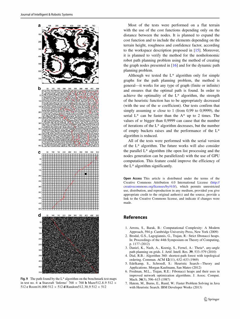
Fig. 9 The path found by the L* algorithm on the benchmark test mapsin test no. 4: a Starcraft ‘Inferno’ 768 × 768 b Maze512 8 9 512 ×512 c Room16 000 512 × 512 d Random512 30 9 512 × 512

Most of the tests were performed on a flat terrainwith the use of the cost functions depending only on thedistance between the nodes. It is planned to expand thecost function and to include the elements depending on theterrain height, roughness and confidence factor, accordingto the workspace description proposed in [15]. Moreover,it is planned to verify the method for the nonholonomicrobot path planning problem using the method of creatingthe graph nodes presented in [16] and for the dynamic pathplanning problem.

Although we tested the L* algorithm only for simplegraphs for the path planning problem, the method isgeneral—it works for any type of graph (finite or infinite)and ensures that the optimal path is found. In order toachieve the optimality of the L* algorithm, the strengthof the heuristic function has to be appropriately decreased(with the use of the w coefficient). Our tests confirm thatsimply assuming w close to 1 (from 0,99 to 0,9999), theserial L* can be faster than the A* up to 2 times. Thevalues of w bigger than 0,9999 can cause that the numberof iterations of the L* algorithm decreases, but the numberof empty buckets raises and the performance of the L*algorithm is reduced.

All of the tests were performed with the serial versionof the L* algorithm. The future works will also considerthe parallel L* algorithm (the open list processing and thenodes generation can be parallelized) with the use of GPUcomputation. This feature could improve the efficiency ofthe L* algorithm significantly.

Open Access This article is distributed under the terms of theCreative Commons Attribution 4.0 International License (http://creativecommons.org/licenses/by/4.0/), which permits unrestricteduse, distribution, and reproduction in any medium, provided you giveappropriate credit to the original author(s) and the source, provide alink to the Creative Commons license, and indicate if changes weremade.

References

1. Arrora, S., Barak, B.: Computational Complexity: A ModernApproach, 594 p. Cambridge University Press, New York (2009)

2. Brodal, G.S., Lagogiannis, G., Trajan, R.: Strict fibonacci heaps.In: Proceedings of the 44th Symposium on Theory of Computing,p. 1177 (2012)

3. Daniel, K., Nash, A., Koenig, S., Fernel, A.: Theta*, any-anglepath planning on grids. J. Artif. Intell. Res. 39, 533–579 (2010)

4. Dial, R.B.: Algorithm 360: shortest-path forest with topologicalordering. Commun. ACM 12(11), 632–633 (1969)

5. Edelkamp, S., Schroedl, S.: Heuristic Search—Theory andApplications. Morgan Kaufmann, San Mateo (2012)

6. Fredman, M.L., Trajan, R.E.: Fibonacci heaps and their uses inimproved network optimization algorithms. J. Assoc. Comput.Mach. 34(3), 596–615 (1987)

7. Hatem, M., Burns, E., Ruml, W.: Faster Problem Solving in Javawith Heuristic Search. IBM Developer Works (2013)

http://creativecommons.org/licenses/by/4.0/

http://creativecommons.org/licenses/by/4.0/


8. Hart, P.E., Nilsson, N.J., Raphael, B.: A formal basis for theheuristic determination f minimum cost paths. IEEE Trans. Syst.Sci. Cybern. 4(2), 100–107 (1968)

9. Hernandez, C., Baier, J.A., Asin, R.: Making A* run faster thanD*-lite for path-planning in partially known terrain. In: Twenty-Fourth International Conference on Automated Planning andScheduling (2014)

10. Khatib, O.: Real-time obstacle avoidance for manipulators andmobile robots. Int. J. Robot. Res. 5(1), 90–98 (1986)

11. Kliemann, L., Sanders, P.: Algorithm Engineering: SelectedResults and Surveys. Springer International Publishing, Basel(2016)

12. Koenig, S., Likhachev, M., Furcy, D.: Lifelong planning A*. Artif.Intell. 155(1–2), 93–146 (2004)

13. Koenig, S., Likhachev, M.: D* Lite. In: Proceedings of the AAAIConference on Artificial Intelligence, pp. 476–483 (2002)

14. Latombe, J.-C.: Robot Motion Planning, p. 651. Kluwer AcademicPublisher, Dordrecht (1991)

15. Niewola, A.: Rough surface description system in 2,5d map formobile robot navigation. J. Autom. Mob. Robot. Intell. Syst. 7(3),57–63 (2013)

16. Niewola, A., Pods ¸edkowski, L.: Nonholonomic mobile robot pathplanning with linear computational complexity graph searchingalgorithm. In: 2015 10th International Workshop on Robot Motionand Control (RoMoCo), pp. 217–222 (2015)

17. Nilsson, N.: Principles of Artificial Intelligence, p. 476. TiogaPublishing Company, Pato Alto (1980)

18. Pods ¸edkowski, L.: Path planner for nonholonomic mobile robotwith fast replanning procedure. In: IEEE International Conferenceon Robotics and Automation, pp. 3588–3593 (1998)

19. Stentz, A.: Optimal and efficient path planning for partially-known environment. In: Proceedings of the IEEE InternationalConference on Robotics and Automation (ICRA ’94), pp. 3310–3317 (1994)

20. Stentz, A.: The focussed D* algorithm for real-time replan-ning. The focussed D* algorithm for real-time replanning. In:Proceedings of the International Joint Conference on ArtificialIntelligence, pp. 1652–1659 (1995)

21. Sturtevant, N.R.: Benchmarks for grid-based pathfinding. IEEETrans. Comput. Intell. AI Games 4(2), 144–148 (2012)

22. Nguyet, T.T.N., Hoai, T.V., Thi, N.A.: Some advanced techniquesin reducing time for path planning based on visibility graph. In:2011 Third International Conference on Knowledge and SystemsEngineering (KSE), pp. 190–194 (2011)

23. Ho, Y.-J., Li, J.-S.: Collision-free curvature-bounded smoothpath planning using composite bezier curve based on voronoidiagram. In: 2009 IEEE International Symposium on Compu-tational Intelligence in Robotics and Automation, pp. 463–469(2009)

24. Zhiye, L., Xiong, C.: Path planning approach based on probabilis-tic roadmap for sensor based car-like robot in unknown environ-ments. In: 2004 IEEE International Conference on Systems, Manand Cybernetics, pp. 2907–2912 (2004)

Adam Niewola received M.Sc. degree in Automatics and Roboticsfrom the Faculty of Mechanical Engineering, Łodz University ofTechnology, Poland in 2011. His researches include mobile robots pathplanning and localization problem, sensor data fusion for orientationestimation, signal filtering and telemanipulation. He was involved inresearch project of a device for measuring femur displacement indamaged hip joint operations.

Leszek Podsedkowski received M.Sc. degree in 1989, PhD degreein 1993 from the Faculty of Mechanical Engineering, TechnicalUniversity of Łodz, Poland. Since 2013 he is a full professor. Heis a manager of the Automation and Robotics Division of Instituteof Machine Tools and Production Engineering and supervisor ofthe specialization of Automatics and Robotics at the Faculty ofMechanical Engineering, Łodz University of Technology. His researchareas include mobile robots path planning, localization and control,telemanipulators, in particular for cardiac surgery, robots constructionand diagnostics and sensor systems for robotics. He was involved inmany research projects, e.g. creation of RobIn Heart, manipulator forcardiac surgery.

l* algorithm—a linear computational complexity graph ... · although the a* algorithm was...

Documents