NASA Contractor Report 189159

,/L// --: '/' / --'_-J

I

F/f7

Probabilistic Structural Analysis Methods

for Select Space Propulsion System

Components (PSAM)

Volume III-Literature Surveys and

Technical Reports

Southwest Research Institute

San Antonio, Texas

April 1992

Prepared for

Lewis Research Center

Under Contract NAS3-24389

National Aeronautics and

Space Administration

('_ASA-C _- 1 ,Jgl_ 9) PROF:A_ ILI ST IC STRUC TUbAl_ Nr_2-247_8

A_ALY_]I'_ _IETnncS FL,'P 5_I..LCT SPACE P_PULS[CN

SV_TE _ £i.;uVCh, Cr, T5 (_At.1). VgLUN_ 3:

LIITRA/UK r 5UPVFYS ANq TECIiNICAL REP'jRTS Unclas

t-in,t] _'p_rt (_o,JthWoSt Re.search Inst.) G]/30 0086861

https://ntrs.nasa.gov/search.jsp?R=19920015555 2018-06-03T13:22:28+00:00Z

Table of Contents

Section

4

5

Literature Review on Mechanical Reliability and

Probabilistic Design

Literature Review on Probabilistic Structural Analysisand Stochastic Finite Element Methods

Level 2 PFEM Formulation Applied to Static Linear

Elastic Systems

A Preliminary Plan for Validation of the First YearPFEM Code

Non-normal Correlated Vectors in Structural

Reliability Analysis

26

107

134

171

Section I

Literature Review on Mechanical Reliability and Probabilistic Design

Prof. Paul H. Wirsching

University of Arizona

February 1985

I. INTRODUCTION

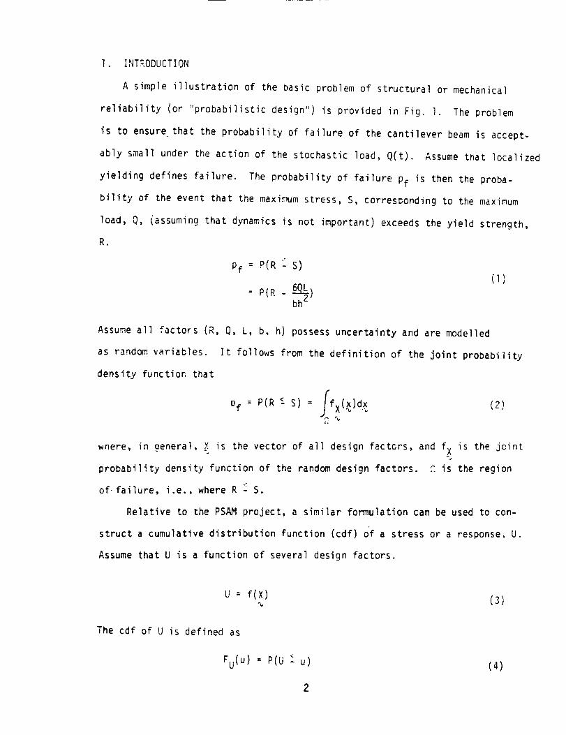
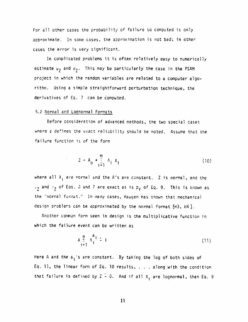
A simple illustration of the basic problem of structural or mechanical

reliability (or :'probabilistic design") is provided in Fig. I. The problem

is to ensure that the probability of failure of the cantilever beam is accept-

ably small under the action of the stochastic load, Q(t). Assume that localized

yielding defines failure. The probability of failure pf is then the proba-

bility of the event that the maximum stress, S, corresponding to the maximum

load, Q, <assuming that dynamics is not important) exceeds the yield strength,

R.

pf = P(R _ S)(1)

6QL)= P(R -

Assume all factoFs (R, Q, L, b, h) possess uncertainty and are modelled

as random variables.

density function that

It follows from the definition of the joint probability

Df : P(R C S) = ffx(_)d_(2)

wnere, in general, ,.Y.is the vector of all design factcrs, and fx is the joint

probability density function of the random design factors. ?. is the region

of- failure, i.e., where R "_S.

Relative to the PSAM project, a similar formulation can be used to con-

struct a cumulative distribution function (cdf) of a stress or a response, U.

Assume that U is a function of several design factors.

U : f(X) (3)%

The cdf of U is defined as

Fu(U) : P(U _ u)

2

(4)

Q(t)

MaximumStress, S

Q(t)

Maximum Load, C!

//_ A j_ mV e, t

b

SEC A-A

Mc 6QL• Maximum Stress S - -I bh 2

• Strength of material z yield strength, R

• Event of failure (R < S)

Fig. 1 An illustration of a simple design problem in which all design factors

(R, Q, L, b, and h) can be considered as random variables.

By analogy, FF(U) can be evaluated by Eq. 2 where '_ = (U _ u).

In the general case, solution of the multi-dimensional integral of Eq. 2 is

impossible in practice. Development of "probabilistic design theory" (or

"structural reliability") is directed towards practical solution to problems

of the type of Eq. i for the purpose of (a) reliability assessment of existing

designs, and (b) development of probability based design requirements.

Presented here is a narrative summary of literature in mechanical relia-

bility(probabilistic design). Contributions are growing and this presentation

is not comprehensive. However, there is confidence that most of the impor-

tant works are cited. The emphasis in this review is for application to the

PS_.I project.

2. HISTORICAL NOTE

The origin of modern probability theory dates back to the 17th century

when an ardent gambler, Chevalier de Mere consulted the Franch mathematician

Blaise Pascal (1623-1662) regardinn a problem about a game of chance. Pascal,

in turn, corresponded with Pierre Fermat (1601-1665). Subsequently, there was

a rapid growth in interest in the mathematics of probability applied to cames

of chance. Karl Gauss (1777-1855) and Dierre Laplac_ (1749-1827) were the

first to find applications in other fields. But serious interest in the syste-

matic application of probabilistic and statistical methods to structural and

r_echanical design did not develop until the mid-1950's.

A brief history of the development of the theory of structural reliability

is presented in the text by Lind, Krenk, and Madsen [LS] and in the Ph.D dis-

sertation of Kjerengtroen [K3]. Parts of the following are quoted from their

work. The history of structural reliability goes back some 50-60 years. The

first phase appears in retrospect as a very slow beginning. Early pioneering

contributions included those of Forsell [F5] and Mayer [M2], and later Basler [BI].

4

M. Prot published several papers (in French) from 1936 to 1951on Statistical

distribution of stresses. And Weibull developed statistical theories of

strength; his name is now associated with an extreme value distribution of

minima [WI, W2]. Later PuQsley [P6] and Johnson [Jl] gave comprehensive

presentations on the theory of structural reliability and of economical desicn.

The modern era of probabilistic mechanical design started after the

Second World War. In October 1945, a paper entitled, "The Safety of Struc-

tures" appeared in the proceedings of the American Society of Civil Engineers.

This histoFical paper was written by A. M. Freudenthal, and the purpose of

it was to "analyse the safety factor in engineering structures in order to

establish a rational method of evaluating its magnitude." It was selecte_

for inclusion with many discussions in the 1947 Transactions ofthe American

Society of Civil Engineers [F6]. The publication of this paper marked the

genesis of structural reliability in the U.S. Most of the ingredients of

structural reliability such as probability theory, statistics, structural

analysis and design, Quality control, existed prior to that time. _leverthe-

less, Prof. Freudentha] was the first to put them together in a definitive

and comprehensive manner. He continued, for many years, to be in the fore-

front of structural reliability and risk analysis as well as fatigue and

fracture studies. A sample of his significant publications on structural

reliability and fatigue are provided in Refs. F7 and F8. Another landmark

paper in structural reliability which began to formalize analysis was written

by Freudentha], Garrelts, and Shinozuka and was published in 1966 IF9].

During the 1960's there was rapid growth of academic interest in

structural reliability theory. Classical theory became well developed

and widely known through a few influential publications such as that of

Freudentnal, Garrelts, and Shinozuka IF9], Pugsley [P5], Kececioglu and

Corm,ier [K2], Ferry-Borges and Castenheta [F2], and Haugen [H3]. However,

professional acceptance was low for several reasons. Probabilistic design

seemed cumbersome, the theory seemed intractible mathematically and numer-

ically. Little data were available. Modelling error was unknown. And

system structural safety analyses seemed extraordinarily complex.

The early 1960's were spent in the search to circumvent these difficulties.

Turkstra IT2] presented structural design as a problem of decision making

under uncertainty and risk. Lind, Turkstra, and Wright [L2] define the

problem of rational design of a code as finding a set of best values of

the load and resistance factors. Cornell [C2] suggested the use of a second

moment format, and subsequently it was demonstrated that Cornell's safety

index requirement ceuld be used to derive a set of safety factors on loads

and resistance. This approach related reliability analysis to practically

accepted methods of design. It has been modified and employed in many

structural standards.

In the ensuing years some serious difficulties with the second moment

format were discovered in the development of practical examples. First, it

was not obvious how to define a reliability index in cases of multiple random

variables, e.g., when more than two loads were involved. More disturbingly,

Ditlevsen [D2] and Lind [L3] independently discovered the problem of invariance.

Cornell's index was not constant when certain simple problems were reformulated

in a mechanical equivalent way. Several years were spent in the search of a

way out of the dilen=na without resolution. In the early 1970's, therefore,

second moment reliability based structural design was becoming widely accepted

although at the same time it seemed impossible to develop a logically firm

basis for the rationale.

6

The logical impasse of the invariance problem was overcome in the early

1970's. Hasofer and Lind [H2] defined a generalized safety index which was

invariant to mechanical formulation. This landmark paper represented a turn-

ing point in structural reliability theory. Contributions, proposed in recent

years, are extentions of the Hasofer-Lind approach which are more sophisticated

mathematically. The era of modern probabilistic design theory which extends

from the early 1970's to the present is reviewed in Section 6.

3. GENERAL REFERENCE TEXTS ON PROBABILITY THEORY AND MATHEMATICAL STATISTICS

There are a large number of text books on the market with the approxi-

mate title of, "Probability and Statistics for Engineers and Scientists."

Two which are recommended for easy reading and reference are those by

Meyer [M3] and Hines and Montgomery [H5]. At a slightly higher level is

the work of Bowker and Lieberman [B4]. Texts on the same level (upper

class undergraduate) written by engineers for engineering practice include

those of Benjamin and Cornell [B3] and the two volumes by Ang and Tang [A2, A3].

Intermediate texts on mathematical statistics include those by Freund [FlO],

Mood and Graybill [M4], and Lindgren [L6]. These present advanced topics,

but in _ form which can be understood by e_gineers having some background.

GesiGns are often selected on the basis of extreme loads stresses cr

strains. Extreme value theory is described in most of the above references,

e.g., both Mood and Graybill [M4] and Lindgren [L6] have discussions on order

statistics. And and Tang's second volume has a chapter on extreme value

theory [A3]. The elementary text by Hahn and Shapiro [H]] on statistical

models in engineering, has a good elementary description of extreme value

theory. However, the most definitive work on this topic, although it is

difficult reading, is the text by Gumbel published in 1958 [G4].

4. MECHANICALRELIABILITYANDPROBABILISTICDESIGNTEXTBOOKSANDGENERAL

REFERENCES

There are a few text books which provide elementary information on

basic probabilisti¢ theory and application to mechanical design. These

include texts by Kapur and Lamberson _KI] and Siddall [$2]. Haugen has

written two books on probabilistic mechanical design, the first was

published in 1968 [H3] and the second appeared in 1980 [H4]. These

texts provide a wealth of practical information, but all fail to

provide comprehensive summaries of modern techniques of reliability

analyses developed in the past ten years.

Two othert_xts which are very useful for many engineering applications

are those of Mann et al. [MI] and Lipson and Sheth [L4]. The former focuses

upon classical reliability models and is an excellent reference for general

applications, . but no design theory. Lipson and Sheth have much useful

information not considered elsewhere.

Advanced text books which treat modern reliability theory include that

of Elishakoff [Ell, Leporati [Ll], and Ang and Tang [A3]. A new text,

not yet published, by Lind, Krenk, and Madsen [L5] is an advanced work which

summarizes the mathematical theory of structural reliability. At this time,

however, perhaps the most highly regarded text is that of Thoft-Christensen

and Baker [Tl].

Other references which provide general summaries of modern design

theory include works by Shinozuka [Sl], Wirsching [WS] in addition to

CIRIA 63 report [R3], and the NBS report of Ellingwood et al. [E2].

B

5. CONFERENCEPROCEEDINGSANDPERIODICALS

In recent years there have been a number of specialty conferences on

structural reliability. The International Conference on Structural Safety

and Reliability ICCOSAR is held every three years, but conference proceed-

ings are not readily available. The 2nd i_ternational Conference on Code

Formats in 1976 was a particularly productive one and its proceedings are

somewhat of a classic [DI]. The ASCE has sponsored a series of four specialty

conferences since 1969 entitled, Probabilistic Mechanics and Structural

Reliability. Proceedings are available through ASCE for the 1979 and 1984

conferences [Pl, P3]. ASCE has also sponsored a specialty conference in

1981 and has published conference proceedings entitled, Probabilistic

Methods in Structural Enqineerin9 which contain some excellent summary

articles [P2].

There is a new journal entitled, Structural Safety _ublished by Elsevier)

strictly dedicated to structural reliability. In addition, the civil engineering

profession has been perhaps most active in the development of modern structural

reliability concepts and the ASCE Journal of Enqineering Mechanics and

Journal of Structural Enaineerin_ contain almost monthly articles on prob-

abilistic design theory. Survey and theme articles published in the Journal

of Structural Enqineerin 9 include a literature review on structural safety

published in 1972 [$4], a series of six articles in 1974 [$5], a series of

eight articles in load and resistance factor design in 1978 [G2], and a

series of four articles in fatigue reliability in 1982 [Fl]. Moreover,

ASCE co_nittees (e.g., the ASCE Administrative Committee on Structural

Safety and Reliability, and its five working committees) have spon-

sored many technical sessions and produced numerous articles.

9

6. A NARRATIVE SUMMARYOF THE DEVELOPMENT AND IMPORTANT REFERENCES OF

"MODERN" MECHANICAL RELIABILITY ANALYSIS.

6.1 Mean Value First Order Second Moment Methods (MVFOSM)

The beginning of modern probabilistic design theory can be arbitrarily

defined by the introduction of the safety index by Cornell in 1969 [C3].

First define the "failure function," Z, or "limit state," so that the event

Z _ 0 is failure. For the example of Eq. 1

Z:R

: R

S

6QL

bh2

(5)

In general, Z will be a function of k random design factors, Xi. An

approximation to the mean value of Z, _Z' and standard deviation of Z, OZ'

can be derived using the first terms of a Taylor's series expansion.

= z(,,) (6)_- %

o_ i'-=1\"_X',/;j_i (7)

where =i and ci are the mean and standard deviations of Xi respectively.

is the vec:or of mean values, (as a rule ofthumb, higher order terms are

significant if the COV's of the variables are greater than 15_).

The safety index defined by Cornell is

_ (B)_Z

In the special case where Z is linear in normal variates (or Z is a

multiplicative function in only lognormal variates), the probability of

failure is exactly

pf = :(-5) (9)

10

For all other cases the probability of failure so computedis only

approximate. In somecases, the approximation is not bad; in other

cases the error is very significant.

In co[_licated problems it is often relatively easy to numerically

estimate UZ and oZ. This may be particularly the case in the PSAM

project in which the randomvariables are related to a computer algo-

rithm. Using a simple straightforward perturbation technique, the

derivatives of Eq. 7 can be Computed.

3.2 Normal a_d Loqnormal Formats

Before consideration of advanced methods, the two special cases

where _ defines the exact reliability should be noted. Assume that the

failure function is of the form

m

Z = A + , A.X. (I0)o i-I l i

where all X. are formal and the A's are constant.l Z is normal, and the

_Z and 'Z of EQS. G and 7 are exact as is pf of Eq. 9. This is known as

the "normal format." In many cases, Haugen has shown that mechanical

design probleps can be approximated by the normai format [H3, H4].

Another conwnon form seen in design is the multiplicative function in

which the failure event can be written as

n a.

A _ X._ "- I (II)i=1 l

Here A and the ai's are constant. By taking the log of both sides of

Eq. II, the linear form of Eq. I0 results, along with the condition

that failure is defined by Z ": 0. And if all Xi are lognormal, then Eq. 9

11

_iven an exact form for pf. This "lognormal format" which forms the

analytical foundation for LRFD[G2], is employed by Wirsching for fatigue

reliability calculations [W5, W7, W8].

Becausea closed form expression for probability results from the

normal or lognormal format, assumptions should be madewherever practical

in the PSAM project to produce this simplified form.

_.3 Advanced Reliability Methods; The Generalized Safety Index

The failure function, Z, of Cornell is defined so that failure is

the event that Z _ O. So defined, the algebraic formulation of Z is not

unique. For example, it would be equally valid to write the Z of Eq. S as

Rbh 2

Z : -6T - Q (12)

A fatal flaw in the safety index of Eq. 8 is that _ is not invariant to

mechanical formulation of the failure function, e.g., the _ of EQ. 8 would

depend upon whether Eq. 5 or Eq. 12 was used.

In 1973 Hasofer and Lind presented a new definition of the safety

index data which overcame the lack of invariance problem [H2]. The scheme

works _ike this. Each "basic design variable" Xi is transformed by sub-

tracting its mean, ui, and dividing by its standard deviation _i" The

"reduced coordinate" xi so defined has mean of zero and standard deviation

of one. Upon substitution into the failure function, a new failure f_nction

Zi(x) is defined in terms of these reduced variables x. The Hasofer-Lind

(H-L) generalized safety index is defined as the minimum distance from the

origin of the reduced coordinates to Zl(_) the failure function in these

reduced coordinates. So defined, the generalized H-L safety index gives

12

the sa:_evalue of _ as the case where the limit state is linear and the

variables are normal. In other cases, the H-L index, _, will differ from

the Cornell index. In summary,the H-L generalized safety index provides

a measureof reliability which is invariant to the mechanical formulation

of the failure function, and gives the samevalue as the Cornell

index special case of the normal format.

The concept of the generalized safety index may play a key role in the

PSAMproject. An estimate of the probability of failure can be madeby

employing Eq. 9 above with the H-L index. Even though no distributional

information is used in the HoL index, probability of failure so defined will

provide a reasonable estimate to the actual probability of failure in many

cases. More generally, Eq. 9 can be used to construct a distribution

function of a response.

Pe!ative to the PSAMprogram, it is important to note that estimates

of the cumulative distribution function (cdf) of functions of randomvariables

can be madeemploying B. Let U be a function of several design factors

U : f(X i) (13)

Tne cdf of Ll is defined as

Fu(u) : P(U : u)

So that by aPalogy, the failure function is Z = U - u.

(14)

To construct the

cdf, several values of u must be chosen, and the computation for B repeated,

but the computations are rapid by digital computer. Wuand Wirsching have

demonstrated this technique on a low cycle fatigue problem [W6].

13

6.4 Advanced Reliability Methods; Rackwitz-Fiessler and Chen-Lind

A principal limitation of the H-L approach is that distributional

information, even if available, is not used in the analysis. In 1978

Rackwitz and Fiess]er suggested a method which extends the Hasofer-

Lind safety index concept to accomodate distributional information of

the design factors [Rl]. Their method transforms non-normal distributions

into "equivalent" normal distributions by adjusting the mean and standard

deviation so that the distribution and density functions of the non-normal

variables and the equivalent normal variables are equal at the design point.

This scheme, an iterative algorithm which converges to a safety index, is

described in references E2, LS, R3, Sl, Tl, and W7. It has been demonstrated

by _Ju that probability of failure using the Rackwitz-Fiessler B in Eq. 9

produces, in many cases, surprisingly good estimates of the probability of

failure L_,_Jr"_.Using a digital computer, the calculations are very fast and

efficient. Again, the R-F method can be employed to construct distribuzion

functions of responses in complicated problems, and therefore may be very

useful in certain aspects of the PSAM. All of these schemes are referred to

as "fast probability integration methods" because they provide a very fast

approximation T.oEq. 2.

An extensien of the R-F scheme was proposed by Chert and Lind [Cl].

This method uses a three parameter equivalent normal distribution. It

was anticipated that this method can produce more accurate methods of

pf than does R-F, but Wu has shown this to be not always true [W9]. In

fact, Wu has developed another advanced method, which employs techniques

of Rackwitz and Fiessler and Chen and Lind to produce a safety index, and

extimates of probabi]ity of failure with significantly less error than

R-F or C-L.

14

6.5 Comments on Methods Which Rely on Higher Order Approximations to the

Limit State

The procedures described above are referred to as "first order _etnods"

because the limit state is approximated as a straight line at the design

polnt. But other advanced methods have been proposed. In general, relia-

bility analysis can be performed by transforming the basic variables, Xi,

to standard normal variables, x i, as suggested by Rosenblatt [R5]

x : (15)

the inverse transformation is

X = Fil [_(x)] (16)

The inverse transformation is substituted into the original failure func-

tion, Z, so that the transformed failure function, ZI, can be formulated

and the safety index computed. Such a procedure is expected to produce

more accurate values of pf, but the inverse transformation can be extremely

complicated.

Improvements to the first order method, suggested by various authors,

typically eFploy a higher order approximation of the limit state. For

example, Ditlevsen developed bounds by inscribing and circumscribing the

limit state with rotational paraboloids [D4]. Horn and Price investigated

the error of the linear approximation by studying an approximating hyper-

sphere with radius corresponding to the mean curvature at the design point [H7].

To avoid the arbitrariness of the choice of a suitable approximating limit

state, Fiessler et al. investigated several possible forms of the quadratic

limit state [F5]. Breitung derived an asymptotic formula for the probability

of failure which considers curvatures in the limit state at the design point

15

[B5]. Tvedt derived two approximation formulas, both which model the failure

surface with a parabolic surface at the design point, which also give an

accurate estimate of pf [T3].

Because a more accurate description of the limit state is used, these

second order methods have the promise of consistantly producing better

estimates of the probability of failure relative to first order methods.

However, these schemes are are more complicated because the formulations

are made on the transformed space and require second partial derivatives

of the transformed limit state function. In the literature, only a few

simple examples have been presented, e.g., Fiessler et al. [F5], Breitung

[B5], Tvedt IT3]. The evidence is not entirely convincing that quadratic

methods could produce consistantly accurate results relative to other methods.

!n summary, it is not obvious at this time that the much more compli-

cated second order methods will be helpful in the PSAM project. Wu has

shown that his first order method works extremely well, and errors in

computing probabilities are almost always acceptably small [W9].

6.6 On the Drawin 9 Board

While it is widely recognized that higher order forms for approximating

the limit state may produce more accurate estimates of probabilities, they

are typically far more complex than linear forms. Wu has developed a linear

limit state algorithm, an extension of the R-F and C-L methods, which is

efficient and accurate [W9]. He also has under development at this time an

advanced version which, based on a few check cases, seems to be faster and

more accurate.

6.7 Reliability Analysis When the Limit State Function Does Not Have a Closed

Form Expression

Reliability methods described above rely on a closed form expression of

the limit state, e.g., Eq. 5. But there are cases where the relationship

16

between the variables is defined only by a co_puter algorithm, e.g., local

strain and fracture mechanics fatigue life prediction, finite element stress

analysis, etc. Wu and Wirsching have presented a method whereby the c_puter

program is run using various combinations of parameter values, and a poly-

nomial approximating the limit state is fitted to the responses [W6]. A

fast probability integration method is then employed to estimate probabilities.

The good news, . no modification of the program which characterizes

physical behavior is necessary.

regard to the PSAM project,

response variable.

The bad news, particularly with

a separate analysis must be done on each

7. APPLICATION OF PROBABILISTIC DESIGN THEORY TO DESIGN CODE DEVELOPEMNT

Probably the largest effort in the U.S. to implement a reliability based

design criteria was the LRFD (Load and Resistance Factor Design) program to

revise the AISC specifications. Work on the development of the new AISC

specifications started in 1969, and it was conducted by M. K. Ravindra and

T. V. Galambos. A comprehensive summary of the theoretical development is

presented in eight papers in the ASCE Journal of the Structural Division,

Sept. 1978 [G2]; historical summary is provided by Galambos [G3]. The

proposed specificati_)ns [P4] are now open for public review and discussion.

After final revision the new rules will be included as an alternate to the

1978 AISC specifications. The lognormal format, employed in LRFD, may be

useful for elementary reliability analyses in the PSAM project. In particular,

a closed form expression for the probability distribution of response is

possible when the random variables (all assumed to be lognormal) can be

factored outside of the stiffness and mass matrices in the static linear

case. Furthermore, the partial safety factor format of LRFD can be employed

if a safety check expression is required.

17

Other well documented efforts to develop probability based design re-

quirements are available. An excellent description of the review and revision

of the National Building Code of Canada is provided by Siu, Parimi, and Lind

[$3]. The NBS report by Ellingwood et al. recommends load factors and load

.combinations compatible with loads in the proposed 198G version of American

National Standard A58 [E2]. Load factors were developed using concepts of

probabilistic limit states design. Both the Ellingwood report and the CIRIA

63 report [R3] provide excellent and comprehensive summaries of techniques

and applications of modern probabilistic design theory. Moreover, Ellingwood,

eta]. [E2] and Galambos and Ravindra [Gl] provide useful data summaries on

material behavior (structural steel at room temperature). The purpose of the

CIRIA 63 report was to review suitable methods for the determination of partial

factors for use in limit state structural codes. Both reports detail the

definition and process for computing the generalized safety index, a technique

which _,ay be very useful in all aspects of the PSAM project. Another very

excellent reference is the Bulletin d'Information ll2, published by the Comite

Europeen du Beton [R2]. Unfortunately, this document is not readily available,

but it does contain major contributions from many of the pioneers of the

development of probabilistic design theory.

8. A NOTE ON MONTE CARLO METHODS

Monte Carlo is employed very effectively to analyze complicated problems

in probability theory, mathematical statistics, reliabi'lity, random process

theory, etc. As a general rule, Monte Carlo analysis tends to be very costly

relative to the accuracy of the results. Therefore, it is commonly used in

18

a research role to verify the performance of more efficient numerical methods.

In the PSAM project it is not likely to be an effective design tool.

Monte Carlo is particularly inefficient for mechanical reliability

problems because accurate estimates of the small probabilities of failure

require very large sample sizes. Efficiency can be improved by discrimina-

tion in sampling or by extrapolating an empirical distribution function;

but generally speaking, advanced reliability methods cited in Section 6 are

far more efficient for the basic reliability problem.

Monte Carlo seems more of an art than a science, and no complete work,

for engineering application, seems to exist. Elementary concepts (how to

sample from various distributions) are presented in Hahn and Shapiro [HI].

Both Ang and Tang [A3] and Elishakoff [Ell have chapters on Monte Carlo

presenting engineering applications. Thousands of papers have been pub-

lished which describe a wide variety of applications. For example, two

elementary works, by this author, describe application to random process

simulation for fatigue analysis [W4], and analysis of peak responses to non-

stationary random forces [W3].

19

LIST OF _IEFERENCES

AI.

A2.

A3.

i °

B2.

B3.

B4,

B5.

CI.

C2.

,13.

DI.

D2.

D3.

D4.

Ang, A. H.-S., and Cornell, C. A., "Reliability Bases of StructuralSafety and Design," Journal of the Structural Div., ASCE, Vol. I00,Sept., 1974

Ang, A. H.-S., and Tang, W., Probability Concepts in Enqineerin 9Planning and Design, Wiley, 1975.

Ang, A. H.-S., and Tang, W. H., Probability Concepts in EnQineerinQPlannin 9 and Design ,, Vol. II, Wiley, 1984.

Basler, E., "Analysis of Structural Safety," Proceedings, ASCE AnnualConvention, Boston, 1960.

Bendat, J. S., and Piersol, A. G., Engineerin 9 Application of Correla-tion and Spectral Analysis, Wiley interscience, 1980.

_enjamin, J. R., and Cornell, C. A., Probability, Statistics and Decisionfor Civil EnQineers, McGraw-Hill, 1970.

Bowker, A. H., and Lieberman, G. J., Engineerin 9 Statistics, Prentice-Hall, i972.

Breitung, K., "Asymptotic Approximations for Multi-Normal Domain andSurface Integrals," Fourth International Conference on Applications ofStatistics and Probability in Soil and Structural Engineering. Uni-versita di Firenze, Pitagora Editrice, 1983.

Chen, X., and Lind, N. C., "A New Method of Fast Probability Integra-tion," Solid Mechanics Division, University of Waterloo, Canada.

Paper No. 171, June, 1982.

Cornell, C. A., "Bounds on the Reliability of Structural Systems,"

Journal of the Structural Division, ASCE, Vol. 93, No. ST., Feb. 1967.

Cornell, C. A., "A Probability-Based Structural Code," Journal of the_nerican Concrete Institute, Vol. 66, No. 12, Dec. i969.

Dialog, Second International Workshop on Code Formats, Mexico City,

Danmarks Ingeniorakademi, Building 373, 2800 Lyngby, Denmark, Jan. 1976.

Ditlevsen, 0., "Structural Reliability and the Invariance Problem,"

Rpt. No. 22, Solid Mechanics Division, U. of Waterloo, Waterloo,Ontario, Canada, 1973.

Ditlevsen, 0., "Evaluation of the Effect on Structural Reliability of

Slight Deviations from Hyperplane Limit State Surfaces," Proc., 2nd

Int'l. Wrkshp. on Code Formats, Mexico City, 1976.

Ditlevsen, 0., "Principle of Normal Tail Approximation," Journal of

Engineering Mechanics Division, ASCE, Vol. I07, Dec., 1981.

2O

El.

E2.

Elishakoff, I., Probabilistic Methods in the Theory of Structures,Wiley-lnterscience, 1983.

Ellingwood, B., Galambos, T. V., MacGregor, J. G., and Cornell, C. A.,"Development of a Probability Based Load Criterion for American Nation-a] Stand A58," NBS Special Publication 577, June, 1980

FI. Fatigue and Fracture Reliability (4 papers), Journal of the Structural

Division, ASCE, Vol. I08, No. STI, Jan. 1982.

F2. Ferry-Borges, J., and Castenheta, M., Structural Safety, LaboratorioNacional de Engenharia, Lisbon, 1971.

F3. Fiessler, B., Neumann, H. J., and Rackwitz, R., "Quadratic LimitStates in Structural Reliability," Journal of the Enqineering Mechanics

Division, ASCE, Vol. I05, Aug., 1979.

F4. First Order Reliability Concepts for Design Codes, Bulletin d'Information

ll2, Comite Europeen du B6ton.

F5. Forsell, C., "Economics and Buildings," Sunt Fornuft, 4, 1924.

F6. Freudenthal, A. M., "Safety of Structures," Transactions, ASCE, Vol.

ll2, 1947.

F7. Freudenthal, A. M., "Safety and the Probability of Structural Failure,"Transactions, ASCE_ Vol. 121, 1956.

F8. Freudenthal, A. M., "Safety Reliability and Structural Design; Journalof the Structural Division, ASCE, Vol. 77, No. 3, Mar. 1961.

Fg. Freudenthal, A. M., Garrelts, J. M., and Shinozuka, M., "The Analysisof Structural Safety," Journal of the Structural Division, ASCE, Vol.92, No. ST1, Feb., 1966.

FIO. Freund, J. E., Mathematical Statistics, Prentice-Hall, 1971.

Sl. Galambos, T. V., and Ravindra, M. K., "Properties of Steel for Use in

LRFD," Journal of the Structural Division, ASCE, Vol. 104, No. ST9,Sept. 1978.

G2. Galambos, T. V., Ravindra, M. K., et al., . a series of eightpapers on load and Resistance Factor Design iLRFD), Journal of the

Structural Division, Vol. I04, No. ST9, Sept. 1978

G3. Galambos, T. V., "The AISC-LRFD Specification-Conception to Adoption,"

Probabilistic Mechanics and Structural Reliability, ASCE, 1984.

G4. Gumbel, E. J., Statistics of Extremes, Columbia Press, 1958.

21

HI.

H2.

H3.

H4.

H5.

H6.

H7.

Jl.

Ki.

K2.

K3.

LI.

L2.

L3.

L4.

L5.

Hahn, G. J., and Shapiro, S. S., Statistical Models in Engineering,

John Wiley, 1968.

Hasofer, A. M., and Lind, N. C., "Exact and Invariant Second-MomentCode Format," Journal of the Engineering Mechanics Division, ASCE, VoI.I00, No. E:.II, Feb., 1974.

Haugen, E. G., Probabilistic Approaches to Design, John Wiley, 1968.

Haugen, E. G., Probabilistic Mechanical DesiQn, Wiley Interscience,1980.

Hines, W. W., and Montgomery, D. C., Probability and Statistics in

EnQineerina and Management Science, Wiley, 1980.

Hohenbichler, M., Rackwitz, R., "Non-normal Dependent Vectors in

Structural Safety," Journal of the EnqineerinB Mechanics Division,

ASCE, Vol. lO0, No. EM6, Dec., 1981.

Herne, R., and Price, P. H., "Commentary on the Level-ll-Procedure,"Rationalization of Safety and Serviceability Factors in StructuralCodes, CIRIA Report 63, Construction Industry Research and InformationAssociation, London, 1977.

Johnson, A. I., Strength, Safety, and Economical Dimensions of Struc-

tures, Statens Konm_itte for Byggnadsforskning Meddelanded, No. 22,

Stockholm, 1953.

Kapur, K. C., and Lamberson, L. R., Reliabilit X in Engineerino DesiQn,Wiley, 1977.

Kecegioglu, D. B., and Cormier, D., "Designing a Specified Reliabilityinto a Component," Proceedings of the Third Reliability and Maintain-ability Conference, Washington, D. C., 1964.

Kjerengtroen, L., Reliability Analysis of Series Structural Systems,Ph.D Dissertation, The University of Arizona, 1985.

Leporati, E., The Assessment of Structural Safety, Research StudiesPress, 1979.

Lind, N. C., Turkstra, C. J., and Wright, D. T., "Safety, Economy,

and Rationality of Structural Design," Proceedings IABSE 7th CongressRio de Janeiro, 1965.

Lind, N. C., "The Design of Structural Design Norms," Journal of

Structural Mechanics, Vol. 1, No. 3, 1973.

Lipson, C., and Sheth, N. J., Statistical Design and Analysis of En-gineering Experiments, McGraw-Hill, 1973.

Lind, N. C, Krenk, S., and Madsen, H. 0., Safety of Structures, tobe published by Prentice-Hall, 1985.

L6. Lindgren, Statistical Theory, Macmillan, 1962.

22

Ml.

M2.

M3.

M4.

M5.

Pl.

P2.

P3.

P4.

P5.

P6.

Rl.

R2.

R3.

R4.

R5.

R6.

Mann, N. P,.,Schafer, R. E., and Singpurwalla, N. D., Methods for

Statistical Analysis of Reliability and Life Data, Wiley, 1974.

Mayer, M., Die Sicherheit der Bauwerke, Springer-Verlag, Berlin, 1926.

Meyer, P. L., Introductory Probability and Statistical Applications,

Addison-Wesley, 1970.

Mood, A. M., and Graybill, F. A., Introduction to the Theory of Statis-tics, McGraw-Hill, 1963.

Moses, F., and Stevenson, J. D., "Reliability-based Structural Design,"

Journal of the Structural Division, ASCE, Vol. 96, Feb. 1970.

Probability Mechanics and Structural Reliability, ASCE, edited by A. H. S.Ang and M. Shinozuka, 1979.

Probabilistic Methods in Structural Enqineering, ASCE, edited by M.Shinozuka and J. T. P. Yao, 1981.

Probability Mechanics and Structural Reliability, ASCE, edited byY. K. Wen, 1984.

Proposed Load and P,esistance Factor Design Specificaiton for Structural

Steel Bui_dinqs, AISC, 1983.

Pugsley, A., The Safety of Structures, Edward Arnold, 1966.

Puosley, A., "Concept of Safety in STructural Engineering," Proceedincs,Ins. of Civil Engineers, l_51.

Rackwitz, R., and Fiessler, B., "Structural Reliability Under Combined

Random Load Sequences," Journal of Computers and Structures, Vol. 9,1978.

Rackwitz, R., "Practical Probabilistic Approach to Design," FirstOrder Reliability Concepts for Design Codes, Comite Europ6en du Beton,

Bulletin d'Information, No. ll2, July, 1976.

Rationalisation of Safety and Serviceability Factors in StructuralCodes, Report 63, CIRIA, Construction Industry Research and Informa-

tion Association, 6 Storey's Gate, London SWIP 3AU, July, 1977.

Ravindra, M. K., and Galambos, T. V., "Load and Resistance Factor

Design for Steel," Journal of the Structural Division, ASCE, Vol.104, No. STg, Sept., 1978.

Rosenblatt, M., "Remarks on a Multivariate Transformation," Annals of

Mathematical Statistics, Vol. 23, No. 3, Sept., 1952.

Rosenblueth, E., and Esteva, L., "Reliability Bases for Some Mexican

Codes," Probabilistic Design of Reinforced Concrete Buildings, Publi-cation SP-31, American Concrete Institute, Detroit, Mich., 1972.

23

Sl.

$2.

$3.

$4.

$5.

Tl.

T2.

T3.

Wl.

W2.

W3.

W4.

W5.

W6.

WT.

Shinozuka, M., "Basic Analysis of Structural Safety," Journal of theStructural Division, ASCE, Vol. 109, No. 3, March, 1983.

Siddall, J. N., Probabilistic EnQineerin_ Desian, Dekker, 1983.

Siu, W. W. C., Parimi, S. R., and Lind, N. C., "Practical Approachto Code Calibration," Journal of the Structural Division, ASCE, Vol.

I01, No. ST7, July, 1975.

"Structural Safety - A Literature Review," Journal of the Structural

Division, ASCE, Vol. 98, rlo. ST4, April, 1972.

Structural Safety (6 papers), Journal of the Structural Division,

ASCE, Vol. 100, No. ST9, Sept., 1974.

Thoft-Christensen, P., Baker, M. J., Structural Reliability Theoryand Its Applic_tions, Springer-Verlag, N. Y., 1982.

Turkstra, C. J., Theor X of Structural Safet X, SM No. 2, Solid MechanicsDivision, U. of Waterloo, Waterloo, Ontario, Canada, 1970.

Tvedt, L., "Two Second Order Approximations to the Failure Probability,"

Det Norske Veritas (Norway) RDIV/20-OO4-S3, 1983.

Wei_ull, W., "A Statistical Theory of the Strength of Materials,"

Proceedings, Royal Swedish Institute of Engineering Research, No. 151,Stockholm, 1939.

Weibull, W., "A Statistical Distribution Function of Wide Applica-

bility," Journal of Applied Mechanics, ASME, Vol. 18, 1951.

Wirsching, P. H., and Yao, J. T. P., "Monte Carlo Study of Seismic

Structural Safety," Journal of the Structural Division, ASCE, Vol. 97,

_o. STY, May, 1971.

Wirsching, P. H., and Light, M. C., "Fatigue Under Wide Band RandomStresses," Journal of the Structural Division, ASCE, Vol. IO6, No.

ST 7, July, 1980.

Wirsching, P. H., "Application of Probabilistic Design Theory to High

Temperature Low Cycle Fatigue," NASA CR-165488, NASA Lewis ResearchCenter, Cleveland, OH., Nov., 1981.

Wu, Y.-T., and Wirsching, P. H., "Advanced Reliability Method for

Fatigue Analysis, Journal of Engineerin 9 Mechanics, ASCE, Vol. llO,No. ST4, April, 1984.

Wirsching, P. H., and Wu, Y.-T., "Reliability Considerations for the

Total Strain Range Version of Strainrange Partitioning," NASA CR174757, NASA/Lewis RC, Cleveland, OH., Sept., 1984.

24

wg.

Wirsching, P. H., and Wu, Y.-T., "A Review of Modern Approaches to

Fatigue Reliability Analysis and Design," ASME Fourth National Congress

on Pressure Vessel and Piping Tehcnology, Portland, OR, June, and pub-

lished in Random FatiBue Life Prediction, ASME, 1983.

Wu, Y.-T., Efficient Algorithm for PerforminQ Fatigue ReliabilitxAnalyses, Ph.D. Dissertation, The University of Arizona, 1984.

25

Section 2

Literature Review on Probabilistic Structura] Analysis andStochastic Finite Element Methods

Prof. Gautam DasguptaColumbia University

May 1985

26

ABSTRACT

The notion of stochastic variables in structural analysis

was introduced by the late Professor A.M. Freudenthal as early as

in 194_. The goal has been to assess structural safety in a

rational fashion. One cannot totally rely on the hypothetical

deterministic assumptions with the pretention that the knowledge

is complete and exact regarding material properties, geometry of

components, and loading. Hence the Probabilistic Structural

A__nalysis M__ethod (PSAM) emerged in order to evaluate structural

performance in real world situations. Along with the advent of

digital computers the finite element method has established

itself to be the singlemost versatile numerical tool for

engineering calculation. Stochastic analysis on the response

database furnished by a finite element scheme is then the most

logical way to carry out relevant reliability calculations for

engineers who are responsible to assure safe functionality of

systems they analyze, design and construct.

Quantitative estimation of failure apprehension can be

obtained by considering stochasticity of both loading and

structural description. The former aspect is treated in random

vibration and will not be addressed here. Available finite

element type formulations with random variables describing

stiffness, mass and damping matrices due to uncertainities in

boundary geometry, initial stress distributions,, material

properties and bounday conditions, are reviewed in this report.

Computational procedure for evaluating the design statistics

(such as the means, variations, correlations, etc.) of mode

shapes, resonant frequencies, buckling loads and non-linear

dynamic respnses are summarized. A list of reference of

important publications is furnished. Comments on outstanding

issues and necessary research is also included herein.

27

i. Introduction

Engineering systems are designed with a variety of materials

and are shaped convenien£1y in order to perform certain

functions. During its service life a system enounters many

different static and dynamic loading conditions. The main

concern that spans from a lay person to a competent designer is

(a) whether the structure will survive, (b) how well the behavior

of the structure would correspond to the required specifications

and, (c) what are the chances of encountering undesirable

circumstances such as cracks and excessive vibrations. Everyone

is interested in the the overall rating of performance as well.

We can immediately detect that the direction of these natural

questions are both quantitative as well as qualitative in

nature. If we consider the entire design procedure to be a

decision making activity, then at each instance we are compelled

to resolve a generic question. What is the chance that certain

criterion will not be met during the life of the engineering

system which is conceived on a design board?

we immediately recognize that the problem in engineering

design analysis is bifocal. First, we must recognize physical

behaviors and secondly, we must examine the extent of our

knowledge regarding these behaviors. In order to answer the

first question, we axiomatize a mathematical model and quantify

applicable physical laws. Then analysis is performed adhering as

closely as possible to exact solutions. Unfortunately, even many

28

timple objects of engineering design analysis are so complex in

geometry that continuum methods succeeded by analytic solutions

reduces to nothing more than text book examples. Thus in

practice, based on the knowledge of systems of rather simplified

geometry, discrete (as opposed to continuum) methodologies are

pursued where the solutions are arrived at in numerial steps

(contrary to analytical methods with closed form expressions).

Computational methods such as finite difference and finite

element techniques thus emerged as very powerful numerical

tools. With the advent of high speed digital computers, it

became possible to carry out a large number of arithmetic

operations leading to the success of those numerical methods

appropriate for dynamic response computation as well as thermal

analysis. Thus the partial differential equations of

mathematical physics, which dictate the motion, thermal behavior,

etc., are reduced to rather simplified solution of algrebaic

equations. The finite element method, which is a means to

spatially discretize the continuum operator that governs the

field variables, became very popular since the material

inhomogeneity, anisotropy, arbitrariness of boundary geometry

could be easily incorporated in the numerical procedures. In

essence, the answer to the first question can be summarized in

terms of applicability of the conventional finite element method.

However, the second question invokes a different branch of

discipline altogether viz. probabilistic analysis and statistical

computations. We have first hand experience that the design

assumptions are quite empirical if not gross to some extent. In

29

reality we are dealing with partial, often quite incomplete and

contaminated information regarding the structure and loading

conditions. Hence it is quite legitimate to attempt to evaluate

differences between the predicted and any possible realistic

responses. Very naturally, concepts like mean values, standard

deviation, probability distributions and exceedence (probability

to exceed the allowable limits) arise within the selected

numerical method i.e., the finite element method. Thus a

conjugation of the finite element procedure (spatial

descretization) with the probabilistic notion of analysis becomes

ineviable in a rational design-analysis environment.

In order to illustrate the aforementioned generalized (to

some extent rather vague) discussion let us consider one of the

most simple problems in structural mechanics. This will also

facilitate the introduction of some definitions like random

variables, stochiastic processes, etc. which are vital to the

appreciation of the cited literature reviewed in the succeeding

chapters.

h

_-.--

I

Q

L -_-Z!__,_ _-

Fig. i.1 Uniaxial Bar Problem

¥

3O

Consider in Fig. I.I a uniform bar of length L, depth D,

width B, subjected to a constant axial stress a. The material

will be taken to be homogenous thus the modulus of elasticity E

will be considered to be constant. Suppose we are interested in

the strain z and elongation U of the member. From basic stength

of materials:

mr_ -- and U = zL = _L (i.I)

E E

Now we shall ask a pertinent question regarding our

confidence in the assumptions leading to the expressions of ¢ and

U in equation (I.i). The first set of questions will address the

loading. How accurately do we know that a is uniform on the end

surfaces? If there is a device which applies the force we can

never be sure that a perfectly uniform stress condition is

imposed. The rational way to proceed will be to estimate

functions Fa(x,y,a) on the left and right faces such that at a

point (x,y) the probability of the applied stress to be less than

a will be given by the value of the function F. At this stage

let us assume that the bar is "perfect" with its stipulated

geometrical dimensions and modulus of elasticity. The resulting

strain distribution ¢(x,y,z) will also now become uncertain as a

consequence of the distribution Fa(x,y,s). Then the pertinent

design quantity to look for, in order to perform an analysis on

the basis of strain, will be Fz(x,y,z,¢), i.e., the probability

distribution function for the strain z. It is interesting to

note that the stochastical strain now becomes a three-dimensional

function even for the corresponding one-dimensional deterministic

31

case. Hence we need to carry out a three-dimensional analysis of

the aforementioned bar of Fig. i.i. In order to utilize an

available finite element computer program we spatially discretize

this static problem. Without any loss in generality and

especially in order to avoid unnecessary complexity let us assume

that the end stresses are so applied that a does not vary with

x. Hence the probability distribution function for a could be

represented in the form Fa(y,_ ). If from our engineering insight

we assume that the resulting strain _ does not vary with x at a

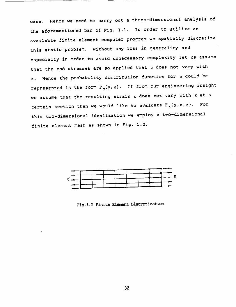
certain section then we would like to evaluate Fz(y,z,¢ ). For

this two-dimensional idealization we employ a two-dimensional

finite element mesh as shown in Fig. 1.2.

-.-.-4m..f

I

Fig. I. 2 Finite El_nent Discretization

32

The objective of the probabilistic finite element procedure within the

context of the problem in Figs. i.I and 1.2 is to evaluate Fz(y,z,_)

when F_(y,a) are given for each end faces.

In the preceeding example we consider the stress, _, loading

(forcing function in the finite element system) to be a

nondeterministic function of x and y. This will be termed to be a

stochastic or random process. A formal definition of a random process

is that f(x) is a random process if f is a random function of a

deteministic argument x. We shall indicate stochastical variables

with a tilda. Thus a random function such as the stress, strain in

the above problem will be random processes, _(y) and _(y,z),

respectively. (Notation introduced in [B-I.43 will be used throughout

this report.)

A dynamic version of the above class of problems, depicted in

Figs. i.i and 1.2, attracted the notice of several researchers.

Therein a structure or any other mechanical system was considered to

be completely deterministic whereas only the forcing function (such as

the earthquake or wind load) was considered to be random processes in

time. This class of problem of deterministic system with random

loading are treated in a special branch of dyamics called random

vibration, refer to [C-1.4]. There are excellent standard text books

on that topic as listed in the reference (section I0).

We can further pursue our question regarding the assumptions in

a U = aLthe formulation leading to ¢ = _ , -_ in equation (I.i). There

are possibilities that during manufacturing of the "real world" bar in

Fig. 1 the chemical process was not exact or perfect hence the modulus

33

of elasticity E may just be almost constant and is indeed a random

function of x,y.and z, i.e. E(x,y,z). Since the manufacturing

processes are quite reliable we expect E to be a narrow band process

implying that the difference in say the maximum and minimum values of

E everywhere will not be too large. Statistically speaking the

dispersion in E will not be enormous. Similarly a realistic (non

ideal) manufacturing proces will incur variation in the depth D and

width B of the bar (refer to Fig. I.I). Thus B and D are to be taken

as stochastic processes: B(z,y) and D(z,x) , respectively. Most likely

the departures _B and _D of the width and depth from corresponding

= + _B similarly D = Do+ _D_ will bemean values B O and D O [B B °

confined within a few percentage points. Now the estimation of

probability distribution function F in terms of F , F , F and F will

not be a simple algebraic task. In fact the deterministic equations

(I.i) may not even be valid for the mean values, i.e.

(1.2)

The stochasticity in material properties and in geometry which modify

the system stiffness is of principal importance here in the estimatior

of randomness for strains, displacements, and any relevant response

quanitity. Published papers, which deal with the estimation of mean

and standard deviations (correlation matrix in the case of correlated

stochastic variables) are reviewed in this report. The finite element

methodology has been the focus in recommending practical solution

strategies which consider randomness and particularly the spatial

variability of stochastic processes in structural systems.

34

2. Problem Statement

We express a finite element form for the equation of motion

of a structure in the symbolic form:

s R = F (2.1)

where: S:

R:

F:

system stiffness operator

system response history

forcing function

For a vector of random processes _ which define the system

S, the corresponding stochastical finite element system of

equation will then be

_ = _ (2.2)

In a generalized probabilistic finite element problem we shall

have:

F " the probability distribution function for basic

uncertain quantities are prescribed.

F : the probability distribution functions for response

quantities are to be calculated.

35

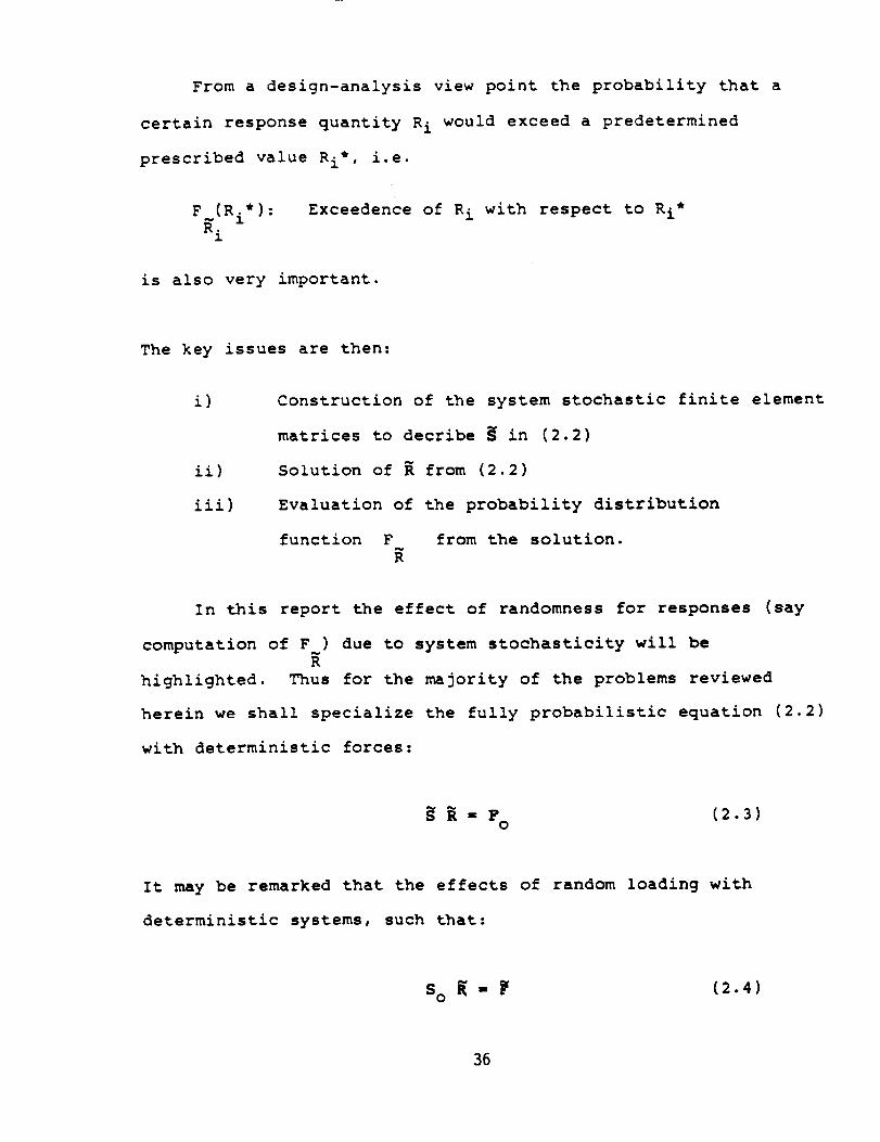
From a design-analysis view point the probability that a

certain response quantity R i would exceed a predetermined

prescribed value Ri* , i.e.

F~(Ri*) :R.1

Exceedence of R i with respect to Ri*

is also very important.

The key issues are then:

i)

ii)

iii)

Construction of the system stochastic finite element

matrices to decribe S in (2.2)

Solution of R from (2.2)

Evaluation of the probability distribution

function F from the solution.

R

In this report the effect of randomness for responses (say

computation of F ) due to system stochasticity will be

highlighted. Thus for the majority of the problems reviewed

herein we shall specialize the fully probabilistic equation (2.2)

with deterministic forces:

R = F (2.3)o

It may be remarked that the effects of random loading with

deterministic systems, such that:

so = (2.4)

36

can be found in various publications on random vibrations.

Research with system stochasticity refer to equation (2.3) are

rather scarce compared to quite a rich literature available on

random excitation. From the practical consideration in the

structural engineering application it is adequate to postulate

narrow band processes for a stochastic quantity Xi" In some

sense of a norm W.one can than write:

I 5x i l<< 1

! x, IIl

(2.5)

[A norm I.I is a quantification where UXil is a real positive

(non-negative) number associated with a physical variable Xi ]

Consequently, it is quite pertinent to propose that the system

components and the responses as well will obey inequalitites

similar to equation (2.5). This naturally makes the pertubation

method very attractive in analyzing the system equation (2.3).

From its incipience the stochastical finite element method

resorted to perturbation expansion in forms of Taylor series

about mean inputs in order to yield required statistics related

to F .

In the sections that follows noteworthy papers which deal

with system stochasticity, refer to equation (2.3), will be

summarized with brief description of solution procedures and

published numerical results.

37

3. Papers of Historical Importance

Boyce in 1961, published a paper of column buckling with

stochastical initial displacement. ("Buckling of a Column with

Random Initial Displacement", Journal of Aero. Sci.). The

eigenvalue problem related to free vibration of structures with

stochastical mass and stiffness matrices was completed in 1968 by

Collins and Thomson ("The Eigenvalue Problem for Structural

Systems with Stochastical Properties", AIAA Journal). The

pertubation method introduced by Collins and Thomson was later

adopted by many researchers, such as Nakagiri and Hisada IN-4.1

to N-4.8]. There latter authors derived the mass and stiffness

matrices by employing the finite element method. The

aforementioned two papers and [C-3.1] [B-3.13 are of historical

significance in the research of structural mechanics problems

with system stochasticity.

From the standpoint of Probabilistic Structural Analysis

Method (PSAM) the first paper the reviewer found of direct

interest is by Mak, and Kelsey, in 1971 titled: "Statistical

Aspects in the Analysis of Structures with Random

Imperfunctions". Cambou in 1972, employed a direct finite

element formulation in first order stochastic analysis for linear

elasticity problems [C-3.23.

Mak and Kelsey [M-3.1] considered the out-of-plane buckling

bifurcation of a column due to uncertainty in the initial stress

distribution. This is the first published mathematical

development with numerical results for any structural problem

38

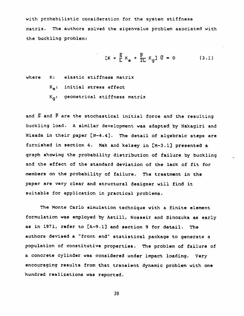
with probabilistic consideration for the system stiffness

matrix. The authors solved the eigenvalue problem asociated with

the buckling problem:

[K + _ K e + _-_ Kg] U = 0 (3.1)

where K:

K e :

Kg:

elastic stiffness matrix

initial stress effect

geometrical stiffness matrix

and S and P are the stochastical initial force and the resulting

buckling load. A similar development was adapted by Nakagiri and

Hisada in their paper [N-4.4]. The detail of algebraic steps are

furnished in section 4. Mak and kelsey in [M-3.1] presented a

graph showing the probability distribution of failure by buckling

and the effect of the standard deviation of the lack of fit for

members on the probability of failure. The treatment in the

paper are very clear and structural designer will find it

suitable for application in practical problems.

The Monte Carlo simulation technique with a finite element

formulation was employed by Astill, Nosseir and Sinozuka as early

as in 1971, refer to [A-9.1] and section 9 for detail. The

authors devised a "front end" statistical package to generate a

population of constitutive properties. The problem of failure of

a concrete cylinder was considered under impact loading. Very

encouraging results from that transient dynamic problem with one

hundred realizations was reported.

39

4. General Procedures for Stochastic Finite Elements

In the existing literature, stochastical analysis of

engineering systems are confined to the first- and second-order,

second-moment approximations. The method calls for the first-

and second-order Taylor expansion of any generic response

quantity in terms of system random variables around the mean

argument. Subsequently the mean and standard deviation of the

response function in question can be estimated. This procedure

is known as the delta method by statisticians. Hitherto emphasis

has been placed on reliability analysis whereby the exceedance

coefficients are estimated on the basis of means and dispersions

of response quantities. A more precise estimation of exceedance

calculation will necessitate the knowledge of higher-order

moments. The existing literature on stochastic finite elements

is rather deficient in evaluating these higher-order moments.

The methodology for the first-order second-moment

approximation is quite complete for linear systems. The second-

order perturbation formulations are rather recent. Even though

the methodology is straightforward and conceptually amenable to

nonlinear dynamic systems, the details of computational strate-

gies suitable for finite element systems especially with a large

number of stochastic parameters cannot be found in existing

literature.

A thorough review of published research in the are of

probabilistic analysis for finite element systems reveals two

major directions. Theoretically, the perturbation formulation

and numerically the Monte Carlo simulation are the only courses

4O

available so far. In this section stochastic finite element

formulations according to the perturbation method is detailed.

The notion of finite element spatial discretization in a

stochastic model on the basis of the scale of fluctuation is also

reviewed here. The Monte Carlo simulation technique is more of a

statistical method hence it is described in the next chapter.

Perturbation Method

The systematic development of the stochastical finite

element formulation according to the perturbation method was

initiated by Nakagiri and Hisada, refer to [N-4.1] - [N-4.8].

They essentially employed the perturbation method [B-I.4] and

reatined up to second-order terms. In order to focus on the

stochasticity of the system, the load vector (the right-hand side

of the equation of equilibrium) was taken to be deterministic.

In this review, the equations furnished by Nakagiri and Hisada

will be rewritten using the notations that appear in [B-4.1]. In

the interest of clarity, indicial notation will be employed

whenever required.

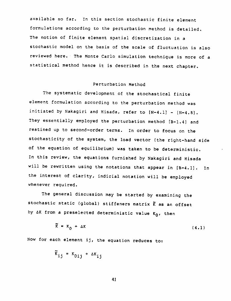
The general discussion may be started by examining the

stochastic static (global) stiffeners matrix K as an offset

by _K from a preselected deterministic value K 0, then

K ffiK 0 + _K (4.1)

Now for each element ij, the equation reduces to:

Kij = K0ij + _Kij

41

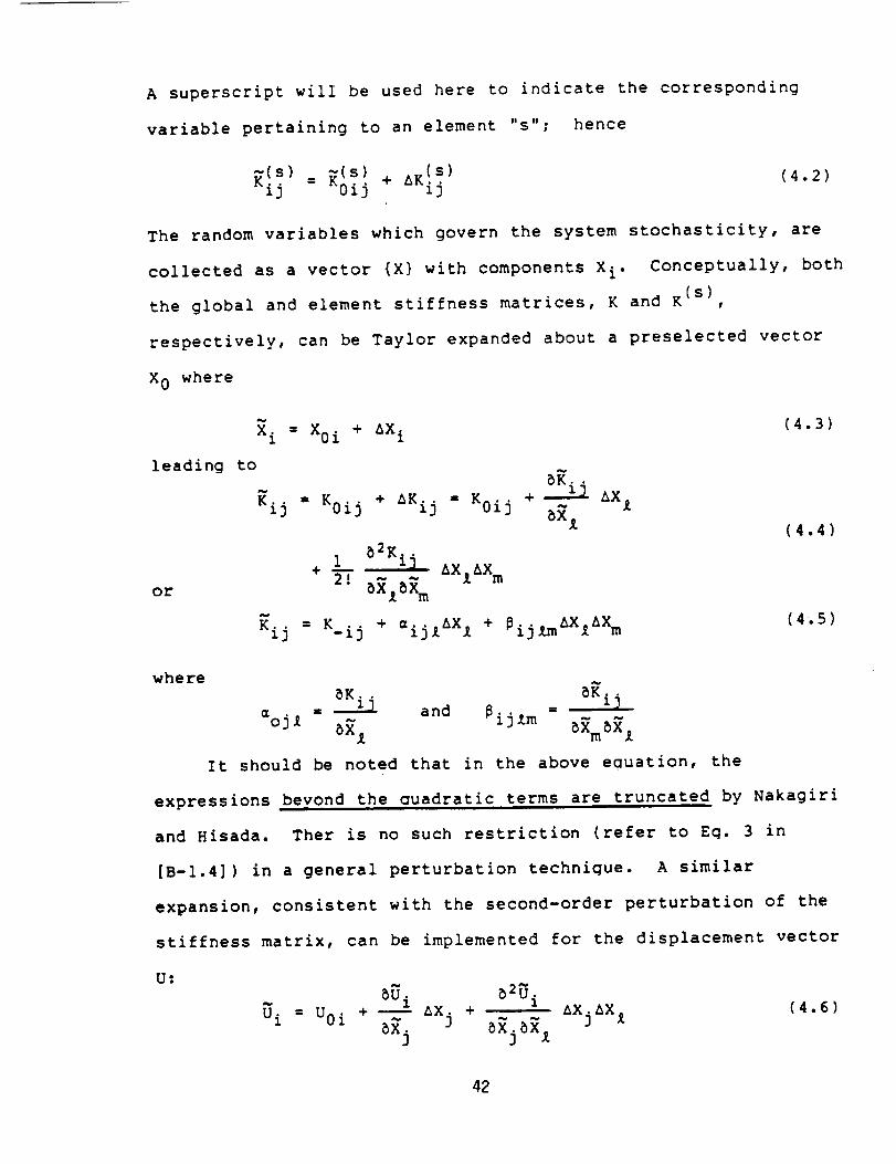
A superscript will be used here to indicate the corresponding

variable pertaining to an element "s"; hence

= cs)13 0ij ÷ AK.. (4.2)ij

The random variables which govern the system stochasticity, are

collected as a vector {X} with components X i. Conceptually, both

the global and element stiffness matrices, K and K (s),

respectively, can be Taylor expanded about a preselected vector

X 0 where

Xi = X0i + AXi (4.3)

leading to

or

Kij = K0ij + _Kij = K0ij + _-_ AX

_2I Kij

+ _ _x_Xm _X_Xm

_ij = K-ij + _ij_AX_ + _ij_mAX_AXm

(4.4)

(4,5)

where

OK.." _ and _i = t3

_oj_ _ j_m B_m_1

It should be noted that in the above ecuation, the

expressions beyond the uuadratic terms are truncated by Nakagiri

and Hisada. Ther is no such restriction (refer to Eq. 3 in

[B-I.4]) in a general perturbation technique. A similar

expansion, consistent with the second-order perturbation of the

stiffness matrix, can be implemented for the displacement vector

U=

Ui = uoi + -- nx. +• 3 5XjSX_ AXjAX_[

(4.6)

42

Now a static finite element system, with a deterministic load F 0

can be solved when the stiffness matrix and consequently the

displacement vector are stochastical in nature. The governing

equation of equilibrium then becomes

Kij_j " F0i (4.7)

Now, substitution of Eqs. 4.6 and 4.5 into the above equationleads to

[K0i j + aij£_X _ + 8ij_m_X1_Xm] •

,2U,j

5X_ 8X_SX m

_X1_Xm] = Foi

One compares the zero-th, first and second degree terms

(4.8)

containing AXe, AXm,

etc. and obtains the following recursive set of equations:

K0ijU0j = F0i (4.9a)

Koij 8_ - =ij_Uoj

82_ iZ •

K0ij _X_5_m - [SijlmUoj ÷ "i3m 8Xj_

(4.9b)

(4.9c)

It is interesting to note that the above system of equations

can be solved once the K 0 matrix is "inverted." Nakagiri and

Hisada remarked that numerical calculation will be faster in

their method as compared to a Monte Carlo simulation since the

latter necessitates a separate inversion at each numerical

realization for the random vector X.

43

_. _2_.Once U0i, .__.I and z are obtained by solving a set of

linear systems of equations _Eg. 4.9), one can compute the

expected value of _. The expected value operator E, when applied

on the Taylor expanded form for _ (Eq. 4.6), one obtains#

~ _i_U. _2

E[Ui] = U0i + _ E[&Xj] + E[&Xj &X_] (4.10)

~ _j__xj

The authors suggested that in a "deterministic" computation with

K0, the stochastic vector X 0 should be chosen to be the mean

of 5. Then

E[_ i] = X0i i.e. E[&X i] = 0(4.11)

This would simplify the expression for the mean U in Eq. 2.10

leading to

_2U i_[u i] = u0i + ~ E[_xj_x l]

_gj_x z

It is convenient to introduce the covariant matrix Cov[X,X] such

that

(4.12)

E[&X i &Xj] = Cov[_,X]ij = Cov[Xi,X j](4.13)

Now the mean displacement can be computed from:

_2U iE[_ i] = U0i + Coy[ ] (4 14)

_j _ XJ ,X_

The second-order Taylor expansion of K and _ in Eos. 4.4 and

4.6 limits up to second-moment terms in the above equation.

Consistent with these second-moment terms in Eq. 4.14, one

evaluates the dispersion of _i in terms of the variance operator

Var[U i ] :

2

Var[U i] = E[U_] - {E[Ui] } (4.15)

44

The second term of the right-hand side in the above equation was

obtained from Eq. 4.14. The first term on the right-hand side is

calcualted retaining only the second-order terms leading to

÷ 2Uoi COy [Xj ,X_]

i i+ -- -- Coy[ ,X_]

5Xj 5X_ _J

(4.16)

Once the expected value E[Ui] and dispersion var[U i ] are obtained

from Egs. 2.14 and 2.16, the corresponding statistics of the

strain _ and stress _ can be obtained by utilizing the strain-

displacement transformation B in terms of the shape

functions N and the constitutive tensor _. The algebra is sum-

marized in Egs. 15-21 in [B-I.4].

The aforementioned general technique, described by equations

4.1 through 4.16, was illustrated by Nakagiri and Hisada in their

first paper [N-4.1] where only the variation of the shape func-

tions were considered. For a triangular meshing, a shape

function N was written in terms of the area coordinates LI, L 2

and L 3 and the nodal point coordinates. This is a standard

finite element procedure and the details can be obtained from

[Z-I.I]. In this first paper, the stochasticity of the nodal

coordinates were considered. An element stiffness matrix K (s) in

an isoparametric formulation was obtained from the corresponding

stochastic strain-displacement transformation matrix _(s), the

constitutive matrix (stress-strain relationship) C (s) as well as

the Jacobian transformation _(s) whose stochasticity is due to

those of the nodal points. Integration over the element in terms

45

of the area coordinates L 1 and L2 yielded:

z(s). // [_(s)]T c(S)_(s)13(s)IdUldn2 (4.17)

where the determinant of _(s) is indicated by I_(s)l. For a

nodal point coordinate (x,y), the Jacobian assumed the form:

(_ a_) (__._7_.__._.__2 _L3 aL2 _3

(4.18)

which was written as

= J0 + AJ (4.19)

The terms in the _(s) matrix involved expressions

a_ a_like _-_ and _ which were obtained as

_yJ

= (_(s)]-i

N N

_N _)N

_)L1 _)L3:

5N aN

aL 1 _Ll

(4.20)

It was then possible to evaluate the =ij_ and _oj_m terms in Eg.

4.5, once the second-order Taylor expansion of I_I , _-x_Nwere

obtained. The authors denoted

where

I_I" IJol+ D1+ D2 (4.21)

- J°l_J12+ J°22_Jll (4.22a)(2.22b)

46

The required inversion of _(s) in Eq. 4.10 was expressed as

D2[_i -_ : (i - - T_ ÷ )

+ (l-Tq T_J21 &Jl

Ii 22 -J011

J021 J01

(4.23)

Finally _ij£' 8ijlm tensors were obtained after Taylor expansion

of x and y up to second-order terms.

An example was illustrated where the nodal coordinates were

taken as stochastic processes defined by a power spectrum. A

homogeneous Wiener-Khintchine relation was assumed for the

correlations Cov[x,x], Cov[x,y], Cov[y,y].

The autocorrelation R(Ix i - xjl )for a homogeneous stochasticity

was obtained in the following form:

- s(X)cos 2klx i - xjldx (4.24)R(IX i Xjl ) : 2 SO

from a given spectrum s(k).

The paper does not present detailed numerical results. The

computational procedure for the =ijX and 8ij_ m tensors are not

discussed either. It should be noted that in a practical finite

element formulation with stochastic variables the computation of

:ijZ and 8ijem

effort.

would demand substantial numerical and programming

47

In their second paper [N-4.2] Nakagiri and Hisada considered

stochasticity in the static stiffness matrix K due to

(i) variation of constitutive properties, where _[X] isi

considered

and

(ii) variation in boundary data.

The general methodology described before is implemented for those

two cases. The paper details out plane stress/strain examples.

These steps are crucial in developing a stochastic finite element

code with plane elements. However, proper adaptation of the

algebraic derivations to general finite element stiffness

matrices (and to mass matrices as well) could lead to the

formulation pertaining to three-dimensional solid and plate or

shell elements. In the interest of focusing on the method the

two-dimensional linear elasticity example will be sketched out

here.

The stochasticity of the constitutive properties was

considered first. For a plane stress/strain element the Young's

modulus E and the Poisson's ratio v were introduced as bivariate

stochastical processes, in the form of E(X) and _(X). The random

vector X is indeed dependent upon the spatial coordinates x I and

x 2 •

The element stiffness matrix is composed of 2x2 submatrices

obtained from two shape functions N i (x_) and Nj(x_), refer to

[Z-I.I] for details. This submatrix can be written in the

following form:

48

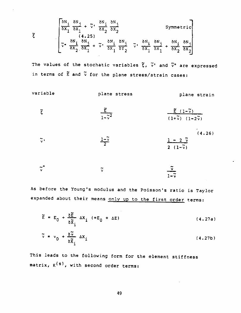
I

%N i _Nj + ;' _Ni _Ni5X 1 5X 1 5X 2 5X 2 Symmetric

(4.25)

The values of the stochatic variables _, _' and _" are expressed

in terms of E and 7 for the plane stress/strain cases:

variable plane stress plane strain

_ _ (_-;)~2

1-v (1+_') (1-2"_)

v' --l-v 1 - 2 72

2 (1-7)

(4.26)

V V

l-v

As before the Young's modulus and the Poisson's ratio is Taylor

expanded about their means only uD to the first order terms:

_ E0 + 5_ ax i ( + aE)5_"_.. =_o

57v 0 +-- aX.

1

(4.27a)

(4.27b)

This leads to the following form for the element stiffness

matrix, K (s), with second order terms:

49

_(s) (s)(s) + _-(s)= K 0 _ _E

+ 5_ (s) (s)AV5_( s )

52 _(S) (s) is) 1 52 _(s) (S} 2+ AE Z_v + (_v

5g(s) 5_(s) 2 5_(s) 2

(4.27c)

[No sum over repeated index "s"]

It is to be noted that the stiffness matrix K is proportional to

52

the Young's modulus E hence _ is zero.

The displacement vector U when perturbed up to second order in

terms of _E and _v leads to

U = U0 + 55 AE(s) _ , Av(s)_(s) +

aE(s) aE(t)

+ 52 _ _E(S) _v (t)

+ _2 _ _v(s ) Av(t)]5;(s'i _;(t)

(4.28)

The expansion for the displacement vector involves summation over

all elements (as described by the superscript "s" and "t"),

whereas that for _(s) pertaining to a particular element s is

described by variations of E and _ in that region.

In the case of a deterministic load vector F 0 the unknown

5O

partial derivatives of _ with respect to E and

by considering terms with AE and 8v in

can be obtained

_U=F 0 (4.29)

leading to:

U0 = [K0]-I F0 (4.30a)

_.__U=- [Ko]-I [_-._KUO] (4.30b)

"___; _ [K0]-i [_ uo]

_-_--- [K0] [~BEBE]

8 2 _ _ _ [K0]-I [SK 8U' + 8_,' 8U

- _ [K0] [ U0 +8 v _ 8_

(4.30c)

(4.30d)

(4.30e)

(4.30f)

The authors suggest the computation of the mean and dispersion

of _ from the above expressions. As claimed by the authors to be

a strong point of their formulation the aforementioned equations

involve the inversion of a single [K0] matrix. (In a Monte Carlo

simulation each realization would demand a separate inversion

of _.)

51

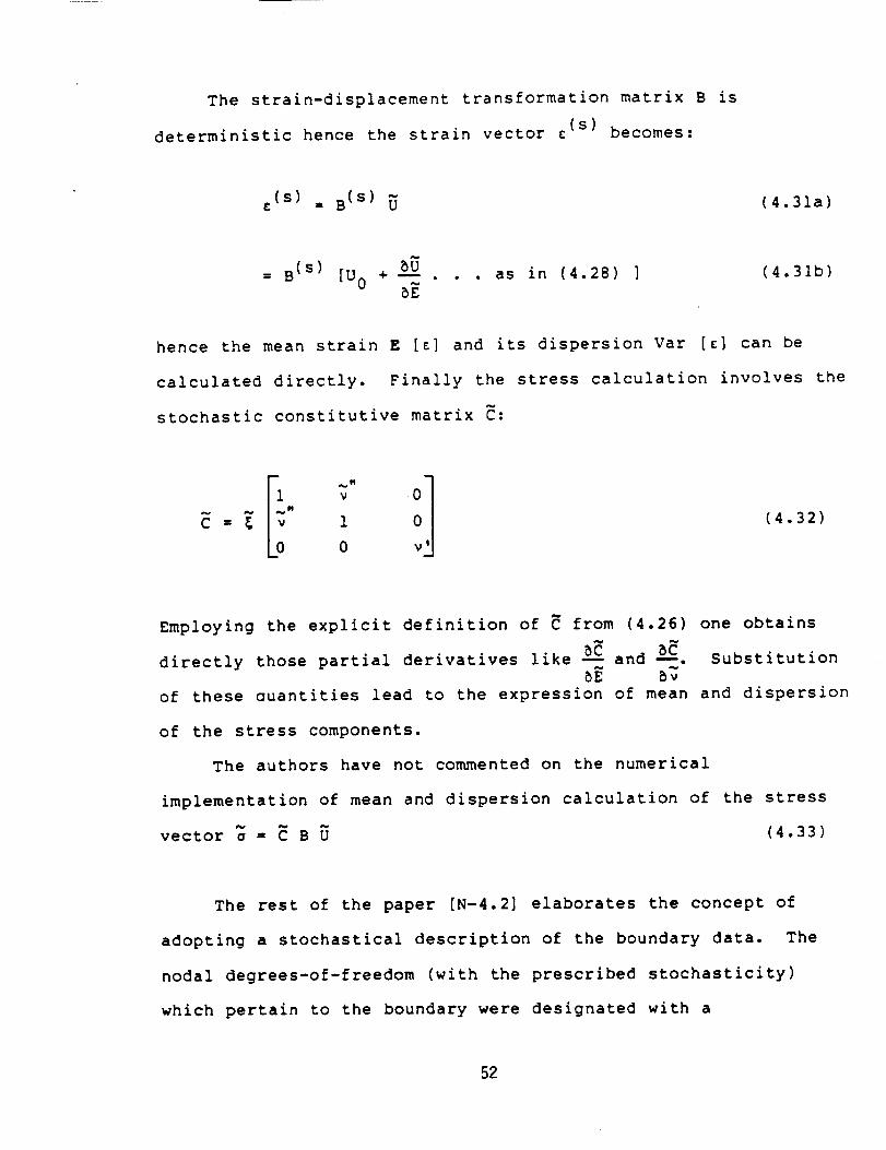
The strain-displacement transformation matrix B is

deterministic hence the strain vector c (s) becomes:

¢(s) = B(S) _ (4.31a)

(s)= B [U 0 +- . . . as in (4.28) ] (4.31b)

hence the mean strain E [_] and its dispersion Var [£] can be

calculated directly. Finally the stress calculation involves the

stochastic constitutive matrix _:

1 v

= 1

0 v

(4.32)

Employing the explicit definition of _ from (4.26) one obtains

directly those partial derivatives like 5-_ and _---_. Substitution

byof these ouantities lead to the expression of mean and dispersion

of the stress components.

The authors have not commented on the numerical

implementation of mean and dispersion calculation of the stress

vector _ = _ B U (4.33)

The rest of the paper [N-4.2] elaborates the concept of

adopting a stochastical description of the boundary data. The

nodal degrees-of-freedom (with the prescribed stochasticity)

which pertain to the boundary were designated with a

52

superscript 2 and the remaining (interior) degrees-of freedom by

i. Then the static stiffness matrix, the displacement and the

load vectors could be partitioned leading to

(21) _(22 (2 (2

(4.34)

Thus the unknown displacement vector (associated with the

interior nodes) _(I) becomes:

5(II [ 1111]-i[ (II_ (12) (4.3si

The authors pointed out that the aforementioned equation

indicated a linear relation between _(I) and _(2) hence

conjectured the possibility of numerical computation of the mean

and dispersion of _(i) from those of the right hand side

quantities from equation (4.35). Finally relevant statistics for

the strain _ and stress _ distributions could be obtained

according to the equations (4.31) through (4.33).

The authors do not include specific numerical examples for

this problem of stochasticity with random boundary data. As in

[N-4.1] and in (4.24) a power spectral density function in the

Wiener-Khintchine form was suggested to account for the spatial

variability of the stochastic quantities. The authors did not

elaborate on numerical computations of means and dispersions of

the stress components from those of the given constitutive matrix

and calculated displacement vector, refer to (4.33).

53

The possibility of extending the perturbation technique

sketched out in [N-4.1] and [N-4.2] for nonlinear problems is

discussed by Nakagiri and Hisada in their third note. A specific

nonlinear constitutive model in the following form was explored:

= f(_) = E _-E b[n{l + l}a-l]

b

(4.36)

A nonlinear constitutive tensor _ could then be assumed in terms

of the effective strain z and effective stress a, which are

defined to be

I 2 + _:2x 2 1

(¢Xl 2 + x3 + _" YXlX2 +

1 2 1 2¢ = _ Yx2x 3 + _ YX2X3)

(4.37a)

and

= f (_) (4.37b)

In principle, for a selected value of _ to be U* the

constitutive matrix _(s) for an element "s" was Taylor expanded

up to second order terms with respect to the stochastical

constitutive variables a and b in (4.36) in the following form:

* (s) * _(s)ll_(S)(u ) = C 0 (u) +-= , _

_a IU

54

+

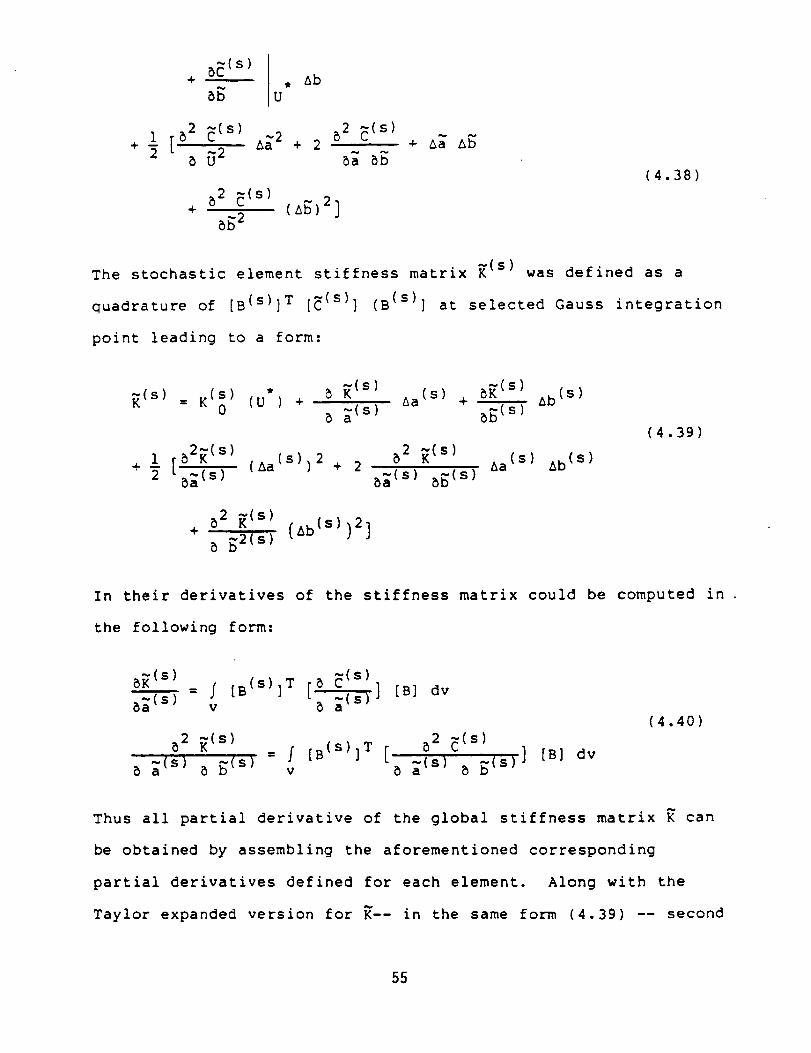
52 _(s) 52 _(s)+ 1 [ _2 + 2 + _ 45

5 _2 5a 55

52 _(S)+ (a_)2]

552

(4.38)

The stochastic element stiffness matrix _(s) was defined as a

quadrature of [B(S)]T [_(s)] (B(S)] at selected Gauss integration

point leading to a form:

_(s) = K(S) * _ _(s) (s) 5_ (s) (s)0 (U) + ~(s) _a + _b

5 a 5b (s)

1 [52K (s) (s) 2 52 _(s) (s) (s)+ _ 5_(s ) (_a ) + 2 _b5_(s ) 55(s ) Aa

52 _(s)+ (ab(S)) 2 ]

5 52(s)

(4.39)

In their derivatives of the stiffness matrix could be computed in

the following form:

5K (s) (s) T 5 _(S)=JIB } [ ]5_(s) v 5 _(s)

[B] dv

52 _(s) 52 _(s)= _ [B(S)]T [ -(S) (S)] [B] dv

5 _(s) 5 _(s) v 5 a 5

(4.40)

Thus all partial derivative of the global stiffness matrix _ can

be obtained by assembling the aforementioned corresponding

partial derivatives defined for each element. Along with the

Taylor expanded version for _-- in the same form (4.39) -- second

55

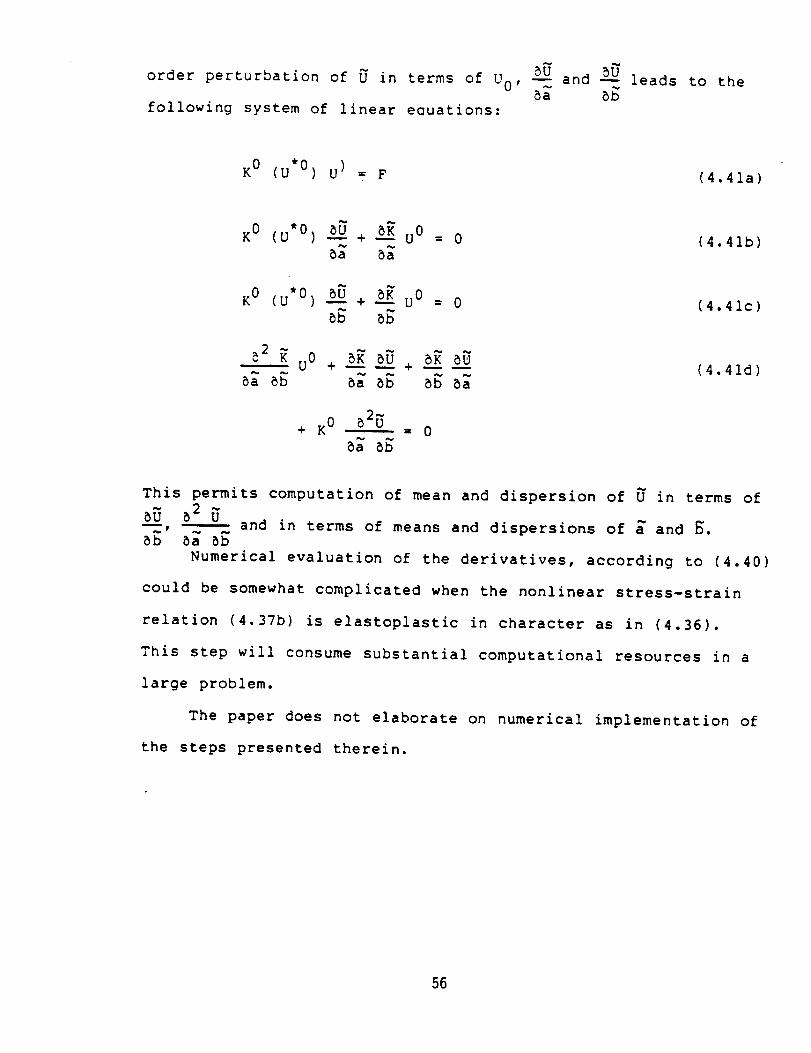
order perturbation of _ in terms of U 0, 5___Uand 5__

following system of linear equations:

leads to the

u*O U)K 0 ( ) = F (4.41a)

u*o _5 _ uoK0 ( ) -- + -- = 0

Ko (u*O) 5___+ ____uo -- 0

U + -- -- +

+ K0 52_ - 0

(4.41b)

(4.41c)

(4.41d)

This permits computation of mean and dispersion of _ in terms of

and in terms of means and dispersions of _ and _._r

Numerical evaluation of the derivatives, according to (4.40)

could be somewhat complicated when the nonlinear stress-strain

relation (4.37b) is elastoplastic in character as in (4.36).

This step will consume substantial computational resources in a

large problem.

The paper does not elaborate on numerical implementation of

the steps presented therein.

56

Nakagiri and Hisada applied the perturbation method to

evaluate safety and reliability for finite element representation

of structural systems. The paper [N-4.5] described a framework

to apply the mean and dispersion of response quantities, as

evaluated in [N-4.1] through [N-4.4], in order to calculate

safety indices. The methodology of the standard reliability

technique applied therein can be found in [W-4.1].

The time history analysis with a stochastical description of

a proportional damping matrix was presented in IN-6]. Some of

the crucial aspects of the latter are described below.

The equation of motion for a damped finite element system

can be written to be..

_ ÷ _ _ + _' * _ = _ct) (4.42)

In the case of proportional damping the damping matrix K' is a

linear combination of the mass and stiffness matrices M, K, in

the form:

_' = _ _ + 5 _ (4.43)

In the specific example [N-4.7] the authors considered determi-

nistic mass and stiffness matrices, then M = M and K = K and

focused attention on stochasticity of the damping matrix via the

random variables a and 5 in (4.43). In the computational step

that was presented in [N-4.7] the authors formulated a broader

class of problems where the damping matrix K' was decomposed into

conventionally C is used to indicate the damping matrix. In

order to avoid confusion with using C for the constitutive matrix

in [B-I.4], a nonstandard notation, K' is used to denote the

damping matrix herein.

57

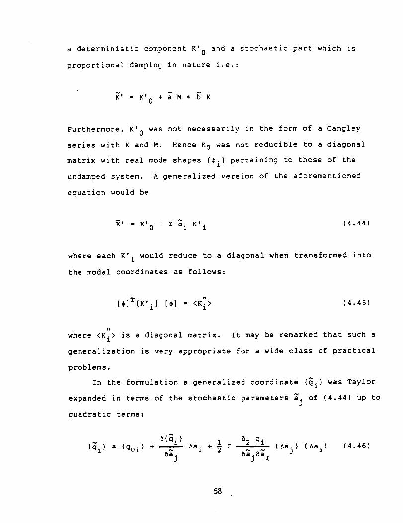
a deterministic component K' and a stochastic part which is0

proportional damping in nature i.e.:

K' = K' + a M + b K0

Furthermore, K' was not necessarily in the form of a Cangley0

series with K and M. Hence K 0 was not reducible to a diagonal

matrix with real mode shapes {#i } pertaining to those of the

undamped system. A generalized version of the aforementioned

equation would be

K' = K' + Z a K' (4.44)0 i i

where each K' would reduce to a diagonal when transformed intoi

the modal coordinates as follows:

[_]T[K' i] [#] = <K[> (4.45)

N

where <K.> is a diagonal matrix.i

generalization is very appropriate

It may be remarked that such a

for a wide class of practical

problems.

In the formulation a generalized coordinate {qi ) was Taylor

expanded in terms of the stochastic parameters aj of (4.44) up to

quadratic terms:

} = {g0i) ÷} 52 qi

aa i + _ £ (aaj) (aa_)

5aj 5_jSal

(4.46)

58

substitution of (4.46) and (4.45) in (4.42) led to the following

set of equations when the modal representation was sought:

"" T , Tm qi + $i k0 $i qi + k qi = $i f (t) (4.47a)

5qi T 5qi 5qi

mi 5-'_7.+ $i k6 ¢i 5"a'_.+ ki] ] ]

" _ k I!.

(4.47b)

m

52qi T _2qi

5ajSa_ + ¢i k0 ¢i 5ajSa_(4.47c)

_2q i

+ k . = - (k". _gi + k_ _qi._qj_a_ 3 _a--_ _'_j'

(note: no sum over repeated indices)

The modal mass and stiffness components were obtained from the

mode shapes as:

T T

#i M $i = Mi and $i K ¢i = Ki (4.48)

The authors solved the aforementioned set of equations by

employing Newmarks implicit time integration scheme ["_ = _."],

Numerical results for a tower with fourteen beam elements

subjected to E1 Centro (1940) NS acceleration input was selected

59

to be the input ground motion.

The statistical computation was simplified by assuming the

random variables _ in (4.44) describing the random coefficient

for the proportional damping matrix to be of zero mean Gaussian

distribution. Thus the required input were Coy [ai,aj]. It

should be noted that the third moment:

E [ai,aj,a _] = 0 (4.49)

and the fourth moment reduced as:

E [ai,aj,a_,a m] --Coy [ai,a j] Coy [a_,am] + (4.50)

Cov [ai,a _] Coy [aj,am] + Coy [ai,a m] Coy [aj,a_]

Numerical results in the form of graphs indicated expectation and

("3-o") bounds of top deflection and the effects of Coy [ai,a j]

on the standard deviation of top deflection for the tower

problem. These are perhaps the only meaningful numerical results

published for dynamic analysis of a finite element system with

stochastic damping matrix.

A column buckling problem [N-4.3] with stochastic

description of the stiffness matrix K and the geometrical

stiffness matrix Kg led to the computation of the buckling load

via the following eigenvalue problem:

[3]

The buckling load is related to the eigenvalue _ and the bent

6O

shape is described by the eigenfunction {_}. It should be

remarked that the content of this paper [N-4.4] is identical with

[C-3.1] where the free vibration problem:

-2 ~

was described. In (4.52) _ and {_] are the stochastical natural

frequency and the mode shape due to stochastic mass and stiffness

matrices, M and K, respectively.

In the note [N-4.4] the authors presented the problem of

buckling of a cantilever beam with the stochastical descriptions

of end restraints as shown in the Fig. 4.1:

- 6.- o

Z ,

,i

r

",,%

"',,,,

Fig. 4.1 Cantilever Beam..Buckling Probl_

The element stiffness matrix for element number 1 which was

attached to a stochastical spring with translational spring

l-s L_ l-cbe

61

~) 61 -121 - s c 2

14 + _ -6L1 -_

symmetric 12 -6L

6L

2L 2

4L 2

(4.53)

The geometrical stiffness matrix for each interior element was

deterministic in nature and was represented in the usual fashion:

(s) El

Kg = 30--_L

m

36m

3L -36 3L

4L 2 -3L -L 2

symmetric 36 -3L

4L 2

(4.54)

In the procedure that followed the element stiffness matrices

were assembled in global matrices [K] and [Kg]. The stochastic

processes, viz [K], _, and {_} were Taylor expanded up to second

order terms with respect to the random parameters _ and _ about

their mean values, sO and cO , respectively. Thus

5c 5s 5_2

02 K )2+ -- (As ]_2

(ac)2 2 --_2_ (_s)(ac)

5s_c

(4.55)

62

since K in (4.53), had rather simple algebraic expressions in

terms of _ and _ evaluation of the partial derivatives,

i.e. =, 8 tensors of [B-I.4], are indeed straightforward. Thus

m

1 0

0

Symmetric

0

0

0 I(4.56a)

2_2_ EI SO

-_ = L-_ (I_S0)3

0

0

Symmetric O1000

(4.56b)

-0 0 0

L 2 0

Symmetric 0

m0

(4.56c )

2_2_ EI CO

_ = _ '(l_Co_3

0 0

L 2

Symmetric

0

0

0

o_

0

0

0m

(4.56d)

Now similar expansion, as in (4.55), for the eigenvalue _ (which

was proportional to the buckling load p p = _L2, E--_-) and the bent

63

shape {7} were carried out in the following form:

7 = ×0 + 5___as + _-_ac ÷5_ 5_

_2 7 1 _2-_ 2+ AS aC + AC

_i" 2 5c2

(4.57)

and

~ ~ 52 7 1 _27 2z = z 0 + 5.._z(as)2 +_ (AS) (ac) (ac) (4 58)

_ _5_" 2 5_2 •

5 2 _ b 2 _ 5 2Note eventhough = 0, _ and __z are nonzero due to

coupling through the implicit "inversion" in a linear eigenvalue

problem. Substitution of (4.53) through (4.58) in (4.51) led to

the following system of linear equations (when the coefficients

of as, ac, (as) 2 2, (ac) are set to zero individually)

([K 0] - k 0 {Kg] ] {z 0} = 0 (4.59a)

(sZ 57 K ) {z o} + (K o -_; 5; g

57k 0 Kg) {_-_} = 0

(sZ 57 K ] (zo) + (Ko -5[ 5[ o

5_X 0 Kg) {_} = 0

r KO) {z } ÷ (,SR 57 K ) {j)'5E2 _'2 0 5[ 5s g 5s

+ (K 0 - k 0 Kg) {_-"'_}5_2" 0

(4.59b)

(4.59c)

(4.59d)

64

52._ _ 5_

_acz

+ (K 0 - X0 Kg) {._} = 0

_2 _K , K )_ g _s _' g _

_c _ g _

* (K0 - _'0Kg) _2 ;= o

(4.59e)

(4.59f)

It is to be noted that computation of partial derivatives such as

_, B2_, etc. in the aforementioned equation, can be carried out

by solving the generalized version of the linear eigenvalue

problems of the form:

x {u) + [A] {z) + {V} = 0 (4.60)

where X (scalar) and {z) (vector) are unknowns but {U) and {V}

(vectors) and [A] (matrix) are prescribed.

The authors presented numerical results for a sample case

and demonstrated the accuracy of this second order perturbation

method.

Finally, the mean the dispersion of _ and {_) were obtained

following the methods in the previous paper [N-4.1], [N-4.2] and

[N-4.3] .

Nakagiri and Hisada also employed the perturbation technique

to the specific cases of stochastic Winkler foundation [N-4.6]

and for random misfit in frame structures [N-4.8]. These two

65

papers are of peripheral importance in describing the general

procedure of the stochastic finite element formulation with

perturbation techniques.

In a conference paper [N-4.9] the authors summarized the

perturbation technique developed in [N-4.1] to [N-4.8].

Numerical results for two specific problems were presented. The

expected value and dispersion of stress intensity factor for an

edge crack with uncertain length were presented in graphical

form. The second problem dealt with mean and standard deviation

of inplane stress developed in a long strip. The authors

compared the results of the first and second order approximations

(where the stochastic processes were Taylor expanded up to linear

and quadratic terms, respectively). In certain cases the

difference of result was quite significant. Hence the authors

recommended the formulation with second order approximations.

66

Handa [H-4.1] initiated stochastical finite element

calculations to enhance design analysis of civil engineering

structures. In a sequence of research reports and conference

papers [H-4.2], [H-4.3], [H-4.4] Handa and his associates

employed finite element analysis technique to estimate expected

values and correlation coefficients of static stresses andJ

displacements for trusses, frames and beam structures.

Stochastical variations of structural section geometry, material

property as well as that of applied loading were considered. All

their discussions were restricted lognormal distribution of

stochastical parameters. For example, for a finite element (s)

the carrying capacity R (s) and any load effect S (s) were assumed

to be lognormally distributed. This facilitated the construction

of the safety margin z defined to be:

z (s) = in R (s) - in S (s) (4.61)

to have a normal distribution.

The presentation [H-4.1] detailed out the first order

perturbation method. The authors remarked that the error

associated with neglecting the higher order terms will not exceed

20% at most. In the interest of brevity the steps are not

repeated here since more detail algebraic development are

presented in this section in equations (4.1) through (4.16).

The authors presented several numerical examples of the

first order second moment formulation. Two noteworthy cases

among those will be summarized here.

67

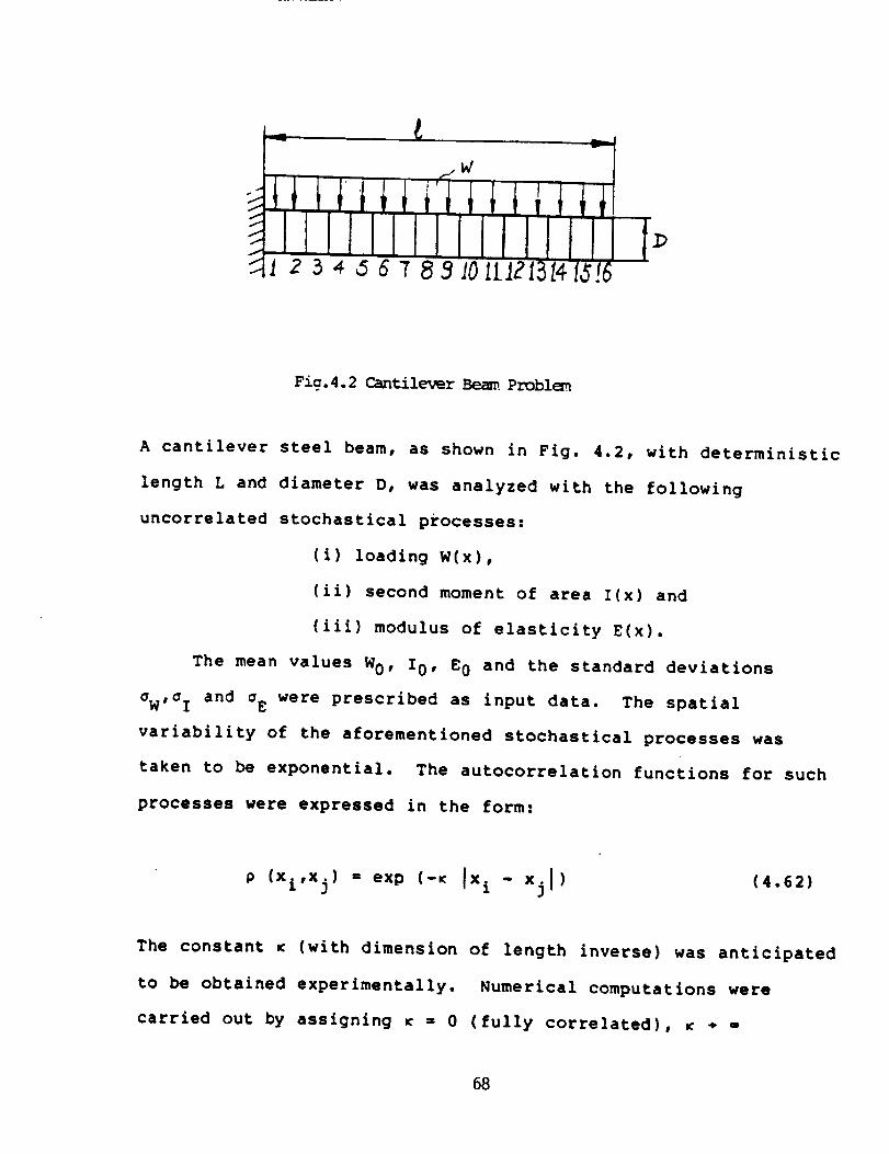
J

f

fw

i 2 _ 4 _ 6 T 8 9 I0 iIiZl,

Fig. 4.2 Cantileu_r Beam Problem

A cantilever steel beam, as shown in Fig. 4.2, with deterministic

length L and diameter D, was analyzed with the following

uncorrelated stochastical processes:

(i) loading W(x),

(ii) second moment of area I(x) and

(iii) modulus of elasticity E(x).

The mean values W0, 10, E0 and the standard deviations

aW,a I and aE were prescribed as input data. The spatial

variability of the aforementioned stochastical processes was

taken to be exponential. The autocorrelation functions for such

processes were expressed in the form:

p (xi,x j) = exp (-¢ lxi- xjl)(4.62)

The constant _ (with dimension of length inverse) was anticipated

to be obtained experimentally. Numerical computations were

carried out by assigning _ = 0 (fully correlated), _ ÷ -

68

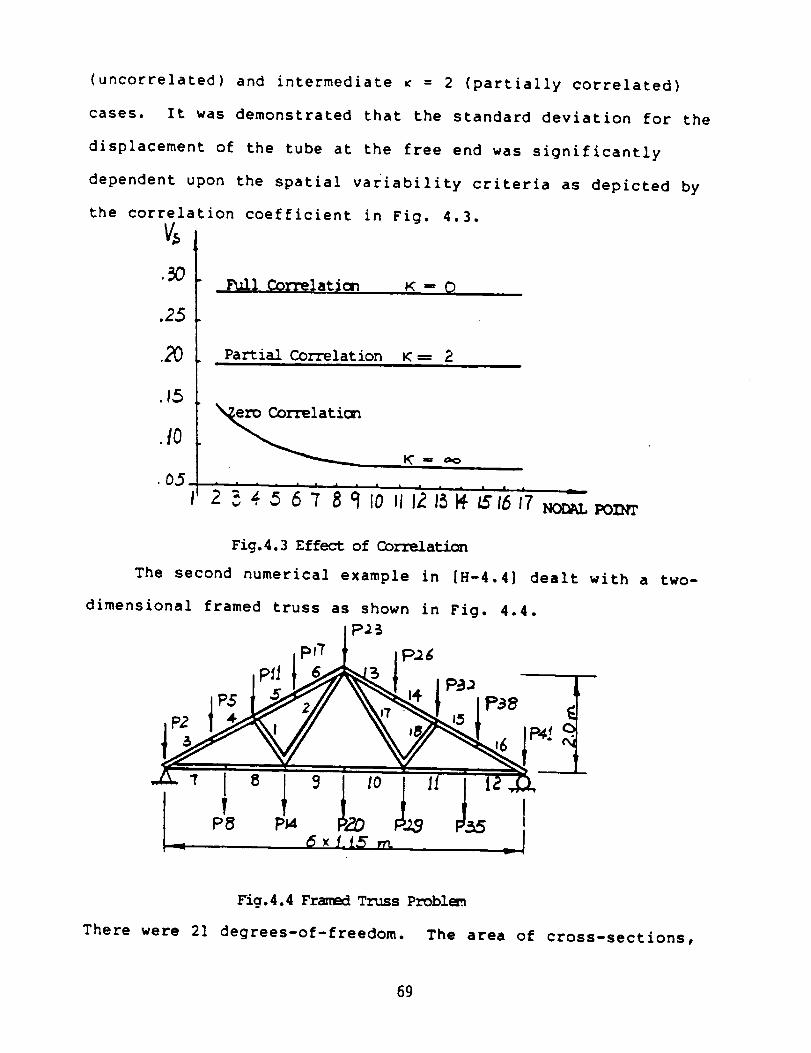
(uncorrelated) and intermediate _ = 2 (partially correlated)

cases. It was demonstrated that the standard deviation for the

displacement of the tube at the free end was significantly

dependent upon the spatial variability criteria as depicted by

the correlation coefficient in Fig. 4.3.

%

Full Corl_latian

Partial Correlation K = 2i

laticm

Fig.4.3 Effect ofCo_ation

The second numerical example in [8-4.4] dealt with a

dimensional framed truss as shown in Fig. 4.4.

p_7 p161 P_

pslP _ 6 _ ;_,

" LL"CP8 P_

two-

Fig. 4.4 Framed Truss Probl_

There were 21 degrees-of-freedom. The area of cross-sections,

69

second moment of areas and the moduli of elasticity were

considered as random variables (with prescribed means and

standard deviations). The stochasticity of fully correlated

loading was expressed by a fully populated 14 x 14 matrix.

Correlation between cross-sectional area, second moment of

inertia and moduli of elasticity i.e. Cov[A,E], Cov[A,I],

Cov[I,E] were taken to be zero. The variance matrix for each

random quantity (associated with those 1B nodes) was thus

obtained in the form of a diagonally dominated banded matrix.

The authors used a computer program [H-4.3] to carry out the

stochastic finite element calculations. Mean values and

covariance coefficients of displacements of all nodes and

stresses in each element were evaluated. The correlation matrix

for stresses was fully populated but decayed with geometrical

distance between two elements.

Scale of Fluctuation Method

Vanmarcke conducted extensive research [V-4.1], [V-4.2],

[V-4.3], [V-4.4], on engineering problems dealing with partial

differential equation of mathematical physics where the

properties of the domain are random processes in the spatial

coordinates. The outstanding contribution was to systemically

develop expressions for local spatial averages of stochastical

quantities as well as variances. For example, in one-dimensional

situation, a stochastic process X i is a "random function" of the

spatial coordinate x= _i(x). In general the expected value for

the product Xi(Xl) and Xi(x2) will be

70

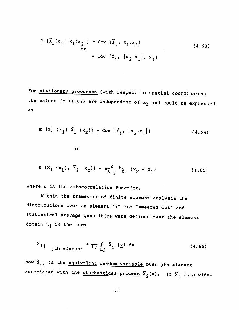
E [Xi(Xl) Xi(x2)] = Coy [Xi' Xl'X2]

or

" I I-COy [X i, X2-X 1 , x ii

(4.63)

For stationary processes (with respect to spatial coordinates)

the values in (4.63) are independent of xI and could be expressed

as

_ {xi (Xl) xi (x2)] = coy [xi' Ix2-xll] (4.64)

or

E [Xi (Xl)' Xi (x2)] = aX 2 P~ (x - x I)i Xi 2

(4.65)

where p is the autocorrelation function.

Within the framework of finite element analysis the

distributions over an element "i" are "smeared out" and

statistical average quantities were defined over the element

domain Lj in the form

= L_ f Xi (x) dv (4.66)Xij jth element Lj ~

Now Xij is the equivalent random variable over jth element

associated with the stochastical process Xi(x). If Xi is a wide-

71

sense stationary process then one defines the mean m_..13

and variance Vat [Xij ] in the form:

E [Xij] -1

~ 2 y~ (Lj)Var [Xij] = o_i xi

(4.67)

in which Y~xi (Lj) described the dependence of the element size on

variance function. From the identities of random signal process-

ing one could write:

x X

_. (x) : f f p_. (Xl-X2) dx I dx 2I 0 0 i

(4.68)

Furthermore, the variance function y_i(x) has the property:

at y (x) = 0 (4.69)YXi (0) = 1 and x÷- _i

The principal contribution of Vanmarcke's presentation is to

define the scale of fluctuation e_i based on the asymptotic

behavior of 7 in the following form:

y_i(x) =-_--as x >> ®_i(4.70)

and

= 2 J p_i(x) dx (4.71)o

72

whenever the above limit (4.70) and the integral (4.71) exist.

An important interpretation of 8_i is in terms of the Wiener-

Kinchine spectral density function g_.(w) wherel

2 f= (x) cos wx dxgxi (w) = _ 0 PXi

(4.72)

and then

= _g_ (0) (4.73)e 'i i

It is important to note that during the selection of mesh size,

for a stochastic process indicated by Wiener-Kinchine spectral

density the characteristic length of a finite element region

should be less than the scale of fluctuation.

Considerable development regarding the scale of fluctuation

for general two-, three- and n- dimensional random processes

could be found in the textbook [V-l.l]. Vanmarcke also presented

very useful approximate formulae for the scale of fluctuations

based on the asymptotic behavior of the correlation function.

Detail mathematical development for unidirectional and two-

dimensional random variates along with useful algebraic

identities could be found in the conference paper IV-4.1].

The journal paper [V-4.2] described in detail the problem of

static deformation of an idealized shear beam shown in Fig. 4.5.

73

Fig. 4.5 Shear Bean Problem

The continuum equation for the deflection v(x) was expressed as

dv(x)= _(x) V(x) (4.74)

dx

in which V(x) was the shear force and a(x) was the shear

flexibility. IFor a rectangular beam of area A(x) and shear

modulus G(x) the shear rigidity is given by G(x)A(x).)

Then

a(x) = ii G(x) A(x)) (4.75)

For the fixed end beam since v(x=0) = 0

x dv x

v(x) = f T_"dx = f0 0

=(x) T(x') dx' (4.76)

74

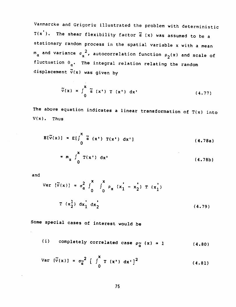
Vanmarcke and Grigoriu illustrated the problem with deterministic

!

T(x ). The shear flexibility factor _ (x) was assumed to be a

stationary random process in the spatial variable x with a mean

me and variance a 2¢ , autocorrelation function P2(X) and scale of

fluctuation ® The integral relation relating the random

displacement _(x) was given by

x

v(x) = f0

(x') T (x') dx' (4.77)

The above equation indicates a linear transformation of T(x) into

V(x). Thus

x

E[_(X)] = E[f _ (x') T(X') dx']0

(4.78a)

x

= m f T(x') dx' (4 78b)a

0

and

X X , , ,

Vat [_(x)] = 2= f f Pa (Xl - x2) T (x I )0 0

T (x) dx I dx 2 (4.79)

Some special cases of interest would be

(i) completely correlated case p_ (x) = 1 (4.80)

Var [v(x)] = a; 2 [ f T (x') dx'] 20

(4.8l)

75

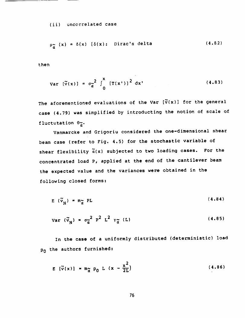
(ii) uncerrelated case

p_ (x) = 6(x) [6(x): Dirac's delta (4.82)

then

X

Var [_(x)] = o_ 2 f [T(x')] 2 dx' (4.83)0

The aforementioned evaluations of the Var [_(x)] for the general

case (4.79) was simplified by introducting the notion of scale of

fluctutation ®~.a

Vanmarcke and Grigoriu considered the one-dimensional shear

beam case (refer to Fig. 4.5) for the stochastic variable of

shear flexibility _(x) subjected to two loading cases. For the

concentrated load P, applied at the end of the cantilever beam

the expected value and the variances were obtained in the

following closed forms:

E (v N) = m_ PL (4.84)

Var (_N) = a_ 2 p2 L2 Y_ (L) (4.85)

In the case of a uniformly distributed (deterministic) load

P0 the authors furnished:

x 2

z [_(x)! = m_ Po r. (x - _--£) (4.86)

76

,., x 1 jxVat Iv(x)] = a_ 2 p02 L2 f dx 10 0

(L-x_) (L-x_).

1 1 (4.87)p_ (x - x 2 ) d x2

Numerical results in graphical forms summarize the variation

of the standard deviation of the end displacement with L/®_, for

various autocorrelation functions such as

Xl-X2 2(4.88a)

X

p_(x I x 2) = exp (-2 I l-X2 2• e }) c4.88b)

X X

p_(xI x2_ = i + 4 I l-x2"_--1 + exp (-4 I l-X21) (4 88c)e E) "

The crucial steps in a stochastic finite element modeling

would then be:

Step - i: Divide a domain D into elements D i and

define the element flexibility quantities as averages:

=i = e S _(x) dv / J dvD i O i

(4.89)

Step - 2: Calculate the mean and covariant matrices:

{real, ma2 ...man} - m~a (i,i,i, ...) (4.90)

and Cov (ai,=j) = Z(4.91)

77

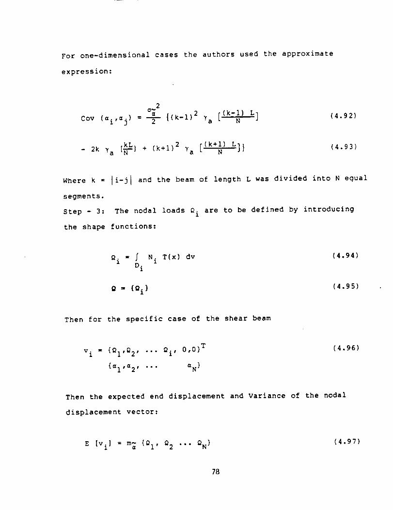
For one-dimensional cases the authors used the approximate

expression:

2O_= 2 (k-l) LI

Coy (ai,= j) = -_- {(k-l) 7a [ N J (4.92)

kL 2 (k+1) L]}- 2k 7a [_-] + (k+l) 7a [ N (4.93)

Where k = li-jl and the beam of length L was divided into N equal

segments.

Step - 3: The nodal loads Qi are to be defined by introducing

the shape functions:

QI" = f Ni T(x) dv

D i(4.94)

Q = {Qi ) (4.95)

Then for the specific case of the shear beam

• = {Q _2 " Q 0 0} Tvl i' ' "" i' ' (4.96)

{_l,a2, ... _N }

Then the expected end displacement and Variance of the nodal

displacement vector:

E [vi] = m~= {QI' Q2 "'" QN } (4.97)

78

Coy [vi,vj ] = QT Z Q (4.98)

The approximation for the covariance matrix Z will depend on a~

and the scale of fluctuation @~ for a selected number of

discretization N.

This paper [V-4.2] will serve as a basis to approximate the

covariance matrix on the basis of scale of fluctuation. In

practical finite element mesh design the scale of fluctuations

for the random field will guide the selection of mesh size.

79

5. Finite Element Stochasticity by Simulation

Astill, Nosseir and Shinozuka [A-5.1] completed the problem

of wave propagation through a random medium by employing a finite

element modeling. Instead of resorting to the pertubation method

to develop the stochastic mass and stiffness matrices the authors

utilized a direct Monte Carlo simulation procedure. This could

be the first published paper where displacement, strain and

stress histories were generated by solving the dynamic euation of

motion of a finite element model with stochastic parameters. The

authors focused their attention on the impact problem and

captured the effcts of randomness in the contitutive properties

on the propagation of stress pulses.

The authors modeled a concrete cylinder with 64 axisymmetric

rings. A quadrant was modeled with 85 nodes. Uniform stress

impact in the form of a triangular shaped pulse was considered.

Graphs of propagation of the stress pulses were presented at

various sections.

Spatial variability of Young's modulus E and density p were

considered. Numerically I00 test samples were recreated by

employing the Monte Carlo simulation technique. Sample

realizations of E and p were plotted against the corresponding

mean values. Deviations from the deterministic case for the

axial stress distribution were also displayed. The means and

standard deviations for the octahedral shearing stress and

miximum shearing stress were calculated using the simulated

8O

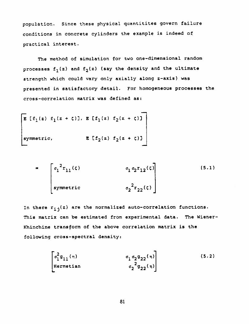
population. Since these physical quantitites govern failure

conditions in concrete cylinders the example is indeed of

practical interest.

The method of simulation for two one-dimensional random

processes fl(z) and f2(z) (say the density and the ultimate

strength which could vary only axially along z-axis) was

presented in satisfactory detail. For homogeneous processes the

cross-correlation matrix was defined as:

i

E [fl(z) fl(z + C)], E [fl(z) f2(z + _)3

symmetric, E [f2(z) f2(z + _)]

I 2 (¢) ala2rl2( ¢aI rll

symmetric a22r22(_)

(5.1)

In there rij(z) are the normalized auto-correlation functions.

This matrix can be estimated from experimental data. The Wiener-

Khinchine transform of the above correlation matrix is the

following cross-spectral density:

a_gll (_)

ermetianala2922(_ 1a22g22(_

(5.2)

81

in which

1 _.l'rij(_) exp (-iDC) d_gij (D) = 2-_

Implentation of FFT (Fast Fourier Transform) based algorithm led

to the simulated variables for homogeneous multivariate Gaussian

processes. The density and crushing strengths were obtained by

simulation and then the Young's modulus for each sample was

calculated by their nonlinear transformation (as is common in

concrete failure analysis).

Computer code to carry out conventional finite element

dynamic calculations was proposed whereas very sophisticated

simulation techniques were used to generate sample finite element

system (mass, stiffness) matrices. In order to adhere to the

prescribed spatial distribution of stochastic processes, which

represent randomness of material properties, the authors

constructed cross-spectral density matrices. The required

mathematical treatment demands thorough training in computational

statistics. It should be remarked that merely ad hoc generation

of realization for system matrices will prove to be completely

useless. In structural reliability assessment the randomness of

the system should be viewed in the light of multi-variate and

multi-dimensional processes [S-5.1]. Gaussian processes with

ARMA (AutoRegressive Moving Average) representation [S-5.2] are

very useful indeed. However, for non-Gaussian stochasticity the

computational complexity and the requirement of theoretical

background in computational statistics could make an analysis

82

almost prohibitive at the existing level of technology.

The aforementioned paper by Astill, Nosseir and Shinozuka

could be the only complete treatment on simulation to be of

practical significance. Engineers undertaking Monte Carlo

simulation for spatially varying random processes will find that

presentation extremely useful. It should be remarked that the

proposed simulation technique demands advanced training in

computational statistics especially in random process analysis.

However, the method to generate statistics (means, dispersions,

etc.) is straightforward once simulation techniques are

mastered. Thus the appropriate steps will be:

(i) to obtain a realization of geometrical and material

properties, etc., according to design statistical

criteria;

(ii) to carry out conventional finite element analysis;

(iii) to generate a population by repeating (i) and (ii)

(iv) to construct mean, covariance matrix, skewness, etc.

from the results of (iii).

The mathematical treatment of Monte Carlo simulation is

arousing new interest since the emergence of parallel processors,

[K-7.13. Research is underway to reformulate simulated finite

element models in order to take the advantage of inherent

parallelism in finite element formulation [S-8.1].

83

6. Papers of Special Interest

Der Kiureghian applied the finite element method to analyze

reliability aspects of linear structures consisting of random

variables [D-6.1 and D-6.2]. Consistant with the notion of

computing the performance index of a structure, a stochastical

vector S is defined to represent the effects of random load andm

random system properties. Any response quantity, like stress,

deformation, can be included in this vector. The paper

elaborates the first-order reliability approach, which relates

the S vector with the allowable "strength" variables vector R

(which typically include design stresses, tolerable deformations,

etc.). Description of the stochastic finite element formulation,

as applied to a linear static system, is extremely clear in the

presentation. It may be remarked the [D-6.1] and [D-6.2] are

perhaps the only two papers in the field of probabilistic finite

elements, where all the conclusions and statements are

substantiated with numeric developments. The papers are devoid

of conjectures and ad hoc promises regarding the computability of

large systems with probabilistic variables. The beam example

presented in these two papers [D-6.1] and [D-6.2] which are

essentially the same, is summarized below.

A beam element in a two-dimensional configuration was

described with three degrees-of-freedom at each end. Associated

with these translational and rotational deformations, the static

stiffness matrix for the uniform section was described by the

following stiffness matrix.

84

Y P

_x

Fig. 6.1 Definition of Two-Dimensional Beam..El_nent

Elements

_2

I_ /'3F

Fig. 6.2 Finite Element Discretization

t El(x)

Fig. 6.3 Fixed-fixed Beam Problem

85

' /

[K(S)] =

where

a b

b d

c e

-a -b

-b -d

c e

f

-C

-e

g

a

b

-C

symme t r i C

12E...../I EAa = L3 sin29 + _ cos28t

d

-e

(6.1)

f

EA EIb = [.--- 12 sine cos.I" J,d

6EIc = -- sin8

L 2

12EI EA

d = 7 c°s2e + _-- sin2'

6EI -- 2EIe = -- cos8 f = 4EI g = __

L 2 _ L _ LL

(6.2)

and E = modulus of elasticity, A = area, I = moment of inertia.

The authors also described the required partial derivatives such

as the ¢ij I tensors, when variability of the material property E

and cross-section A or second-moment of the area I are to be

accounted for. The "form" of the matrices remain the same.

the case of the 5K(S)5-'-_ calculation, the ij-th element can be

directly obtained as _ K(S)ij. Simplified expression for

DR( s )

In

can be written with a = E cos2e, b = { sin�cose, d =

__E sin 28 and c = e = f . g = 0, in (6.1). Similar calculations

_ 5K(s )are possible for-_ with a = ._ sin2e, b-- ._ sin.cos.,

L- L "_ L L L

in (6.1)

The aforementioned formulation does.not permit the

possibility of random description of the nodal point

86

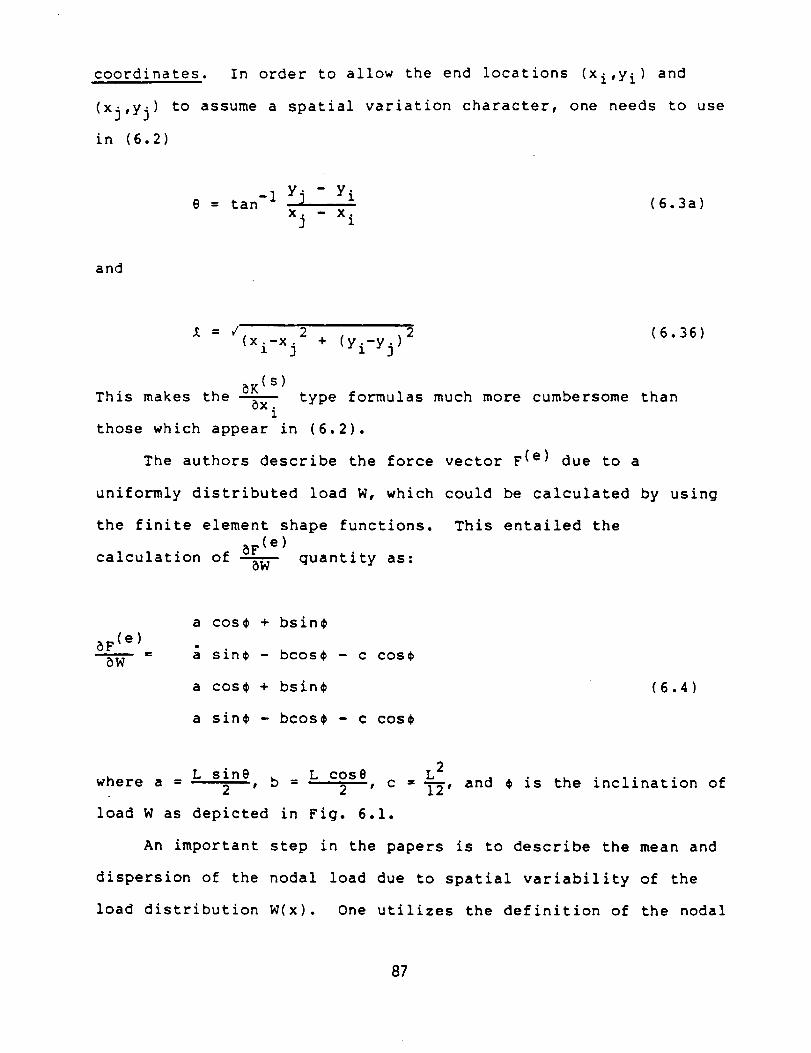
coordinates. In order to allow the end locations (xi,Y i) and

(xj,yj) to assume a spatial variation character, one needs to use

in (6.2)

-i - Yi8 = tanx. - X.3 i

(6.3a)

and

= / 2 2 (6.36)

(xi-x j + (yi-Yj)

_K (s)This makes the 5x. type formulas much more cumbersome than

l

those which appear in (6.2).

The authors describe the force vector F (e) due to a

uniformly distributed load W, which could be calculated by using

the finite element shape functions.

calculation of _F(---_e)5W quantity as:

This entailed the

(e)5F

5W

a cos_ + bsin#

sin# - bcos# - c cos#

a cos_ + bsin#

a sin# -bcos# - c cos#

(6.4)

L sin8 L cos8 L 2

where a = 2 , b = 2 , c = i'-_'

load W as depicted in Fig. 6.1.

and _ is the inclination of

An important step in the papers is to describe the mean and

dispersion of the nodal load due to spatial variability of the

load distribution W(x). One utilizes the definition of the nodal

87

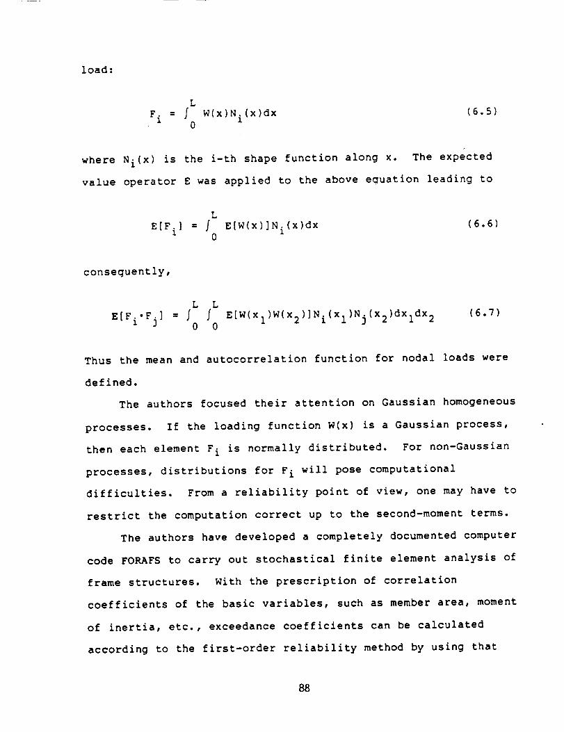
load:

L

Fi = f W(x)Ni(x)dx (6.5)0

where Ni(x) is the i-th shape function along x. The expected

value operator E was applied to the above equation leading to

L

E[F i] = ./0

E[W(x)]Ni(x)dx (6.6)

consequently,

L L

E[Fi'Fj] = _0 _0 E[W(Xl)W(x2)]Ni(Xl)Nj(x2)dXldX2 (6.7)

Thus the mean and autocorrelation function for nodal loads were

defined.

The authors focused their attention on Gaussian homogeneous

processes. If the loading function W(x) is a Gaussian process,

then each element F i is normally distributed. For non-Gaussian

processes, distributions for F i will pose computational

difficulties. From a reliability point of view, one may have to

restrict the computation correct up to the second-moment terms.

The authors have developed a completely documented computer

code FORAFS to carry out stochastical finite element analysis of

frame structures. With the prescription of correlation

coefficients of the basic variables, such as member area, moment

of inertia, etc., exceedance coefficients can be calculated

according to the first-order reliability method by using that

88

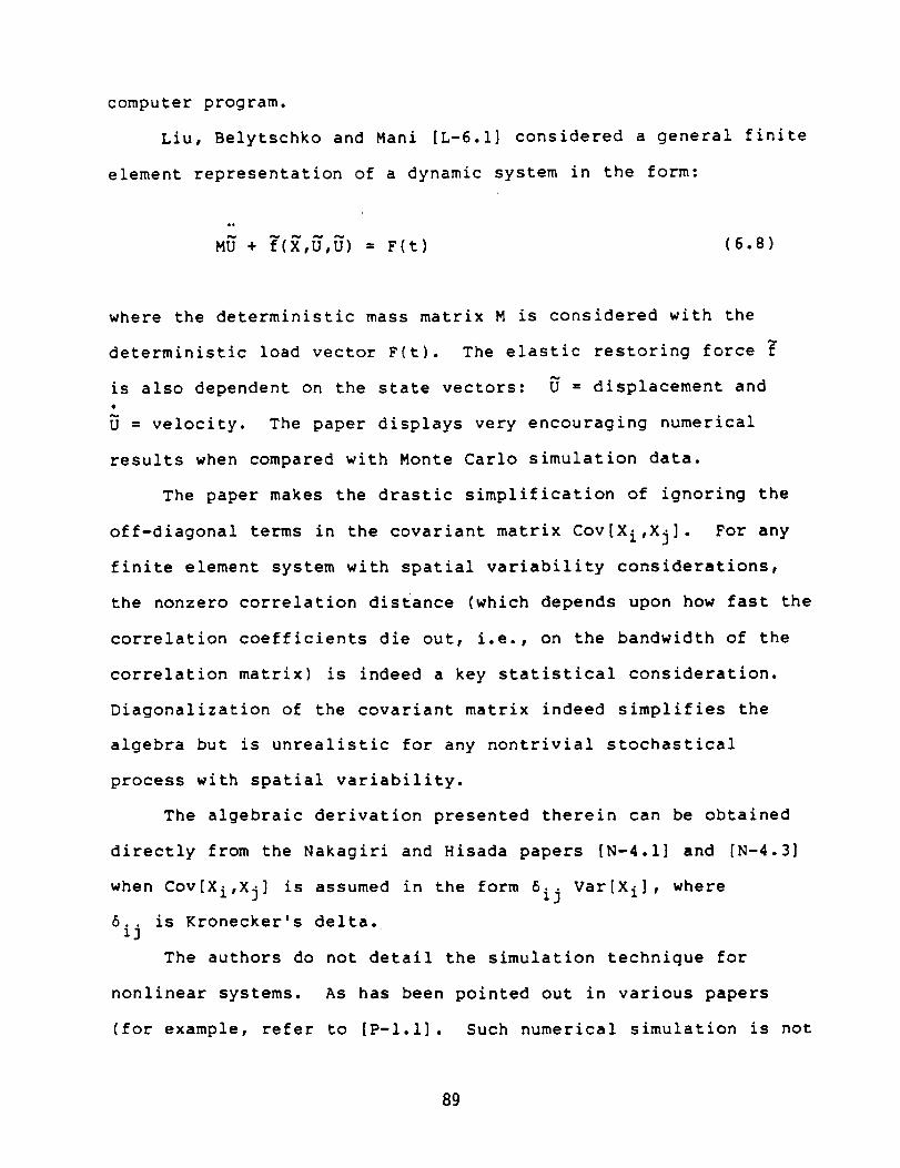
computer program.

Liu, Belytschko and Mani [L-6.1] considered a general finite

element representation of a dynamic system in the form:

where the deterministic mass matrix M is considered with the

deterministic load vector F(t). The elastic restoring force

is also dependent on the state vectors: U = displacement and

= velocity. The paper displays very encouraging numerical

results when compared with Monte Carlo simulation data.

The paper makes the drastic simplification of ignoring the

off-diagonal terms in the covariant matrix Cov[Xi,Xj]. For any

finite element system with spatial variability considerations,

the nonzero correlation distance (which depends upon how fast the

correlation coefficients die out, i.e., on the bandwidth of the

correlation matrix) is indeed a key statistical consideration.

Diagonalization of the covariant matrix indeed simplifies the

algebra but is unrealistic for any nontrivial stochastical

process with spatial variability.

The algebraic derivation presented therein can be obtained

directly from the Nakagiri and Hisada papers [N-4.1] and [N-4.3]

when Cov[Xi,Xj] is assumed in the form 6ij Var[Xi], where

6.. is Kronecker's delta.13

The authors do not detail the simulation technique for

nonlinear systems. As has been pointed out in various papers

(for example, refer to [P-I.I]. Such numerical simulation is not

89

exactly a routine procedure. Secondly, the assumption of

Gaussian distribution for spring constants as in the paper [L-

6.1] (when the possibility of negative stiffeners is acceptable

as a realization) is quite questionable. The paper, at best,

could serve as an example to test out a code under the

aforementioned stringent restrictions of covariant matrix to be a

diagonal one.

In this category of papers of special interest the most

original contribution is by Contrearas, [C-6.1]. The state space

representation of dynamic response for a stochastic finite

element system was conceived to be a finite dimensional Markov

process. The mathematical treatment is elegant and practical

even though rather involved. Algebraic details of the paper will

be summarized in the review of advanced methods. The following

key steps are provided to establish a resemblance of time

marching scheme in finite element temporal solution to a Markov

process (where the present state depends only on the previous one

not on the entire past history).

The author proposed the state vector _ to house the random

variables X,besides the usual case of displacement _ and velocity

U. Thus

The equation of motion of a stochastical dynamic system was

written

(6.9)

90

Y = f[_, t] + G[_, t] Wr (6.10)

in which f is the discrete operator describing the dterministic

equation of motion, G is to represent the contribution of a unit

white noie and W is a white noise. The stochastic vector

differential eguation (6.10) corresponds to Ito's form [A-I.I].

The following temporally discrete form was then obtained:

(in+ I) -% _(tn), in+ I, tn}

+ F(_(tn), in) W(tn+ I)

where the discrete operators % and F were obtained in terms of

the finite element mass, damping and stiffness matrices.

Finally, the unknown vector _ was estimated according to Kalman

filtering method.

91

7. Outstanding Issues and Recommended Research

The major computational concern for a successful execution of

a finite element code with system stochasticity could be assessed

separately for the two separate techniques, viz. the simulation

and the perturbation (and related) methods.

(i) Monte Carle simulation demands the execution of a

deterministic conventional finite element code many man_ times.

Each input realization (like material properties for each

element, boundary node coordinates, temperature distribution,

etc.) is required to be generated by a statistical package

independent of the finite element program. A number of paper

mainly authored by Shinozuka and his associates, [S-7.1], address

the question of simulation in design-analysis for structural

engineering problems. The theoretical background for spatially

uniform multi-dimensional and multivariate Gaussian processes is

quite complete. There are some computer programs available for

research purposes which are suitable for finite element models

with limited number of degrees-of-freedom. There is indeed a

need to develop robust versions of these simulation programs.

In the case of nonGaussian and nonstationary processes

research work is urgently required for the successful development

of simulation algorithms. There is hardly any documented

statistical package on the market in order to generate Monte

Carlo database for arbitrary distributions (which could be

prescibed in tabular observations) particularly suitable for

discrete structural analysis.

There is no available dynamic finite element code which is

92

integrated with a simulation procedure. Engineers, who are

trained in computational mechanics and simultaneously possess

working knowledge in applied statistics should be entrusted to

develop such a statistical front end to a finite element computer

program.

Computers with pipeline architecture and those aided with

parallel processors can carry out repeated deterministic

calculations of simulation in a faster, more accurate and much

more economical fashion, refer to [K-7.1]. The Computational

Statistics group of the Society for Industrial and Applied

Mathematics (SIAM) organizes meetings to present the state-of-

the-art procedures on simulation. Attention is drawn to those

highly theoretical and analytically oriented formulations for

Monte Carlo technique. Useful and practical computational tools

for discrete realizations (as demanded in a finite element input

data stream) could be developed on the basis of the

aforementioned modern mathematical research.

(ii) A direct finite element modeling on a stochastic input

database invariably necessitates a Taylor series expansion at

certain stages of computation. Thus the perturbation principle

is quite inherent in such formulaions. In various presentations

computation of the deviator such as aK [= K-K0], refer to

[B-I.4], or the derivatives with respect to random variables

such as 5K/SXi become essential. This will demand rewriting of

stiffness routines in a conventional finite element computer

code. These routines are much more lengthy, especially when

higher derivatives such as 8ije m - 52Kij/_X_SX m are required.

93

For example, in simple truss problems with stochastic nodal point

coordinates, the expression for the derivative of the element

stiffness matrix K (s) with respect to nodal coordinates xi,Yi,

etc., involves lengthy expressions in terms of trigonometric

inverse functions and their derivatives. The chore to hand

calculate such derivatives and then to develop FORTRAN

subroutines will be extremely time consuming for complicated

finite elements, such as shell elements.

The reviewer himself uses a computer algebra program SMP

(Symbolic Manipulation Program), [S-7.2], to formulate finite

element stiffness matrices and to evaluate derivatives with

respect to the algebraic variables in the stiffness routines.

The Taylor expansion routine in SMP is quite handy. It is

possible to obtain readily the algebraic expressions of the

stochastic stiffness matrix _ expanded about the mean K 0 when the

closed form expression for K (s) is prescribed. It is very

strongly recommended that attention is paid to integrate finite

element FORTRAN program with algebraic manipulating softwares in

order to develop versatile computer code for Probabilistic Finite

Element Method (PFEM). It is to be recognized that initial

experience with the computational philosophy of SMP would demand

a substantial research effort. In the long run, the code

development activities could be expedited for PFEM and PSAM

programs when those powerful algebraic software tools are

implemented.

In selecting the computer algebra program the reviewer

recommends SMP over another similar package called MACSYMA. From

g4

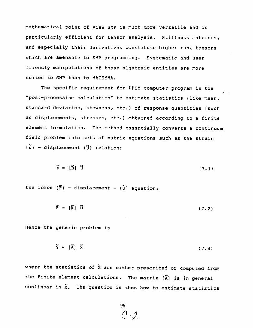
mathematical point of view SMP is much more versatile and is

particularly efficient for tensor analysis. Stiffness matrices,

and especially their derivatives constitute higher rank tensors

which are amenable to SMP programming. Systematic and user

friendly manipulations of those algebraic entities are more

suited to SMP than to MACSYMA.

The specific requirement for PFEM computer program is the

"post-processing calculation" to estimate statistics (like mean,

standard deviation, skewness, etc.) of response quantities (such

as displacements, stresses, etc.) obtained according to a finite

element formulation. The method essentially converts a continuum

field problem into sets of matrix equations such as the strain

(_) - displacement (5) relation:

c = [g] U (?.I)

the force (F) - displacement - (5) equation:

= [K] U (7.2)

Hence the generic problem is

= ¢?.3)

where the statistics of X are either prescribed or computed from

the finite element calculations. The matrix [A] is in general

nonlinear in _. The question is then how to estimate statistics

95

of _ for a large correlated [A]. The complexity of such

expressions like (7.3) can be readily witnessed even in a linear

elastostatic problem where the entries in the element stiffness

matrix is a highly nonlinear function in stochastic Poisson's

ratio. It is a significant computational task to obtain the

numerical values of correlation coefficients for the elements of

stiffnes matrices, when the probability distribution function of

the Poisson's ratio is prescribed, is a significant numerical

task. Attention should be focused on developing a computer

program which could yield such statistics under general

nonGaussian prescriptions of fundamental stochastical variables.

The final answer sought from a PFEM computer program is the

prediction for exceedence. Reliability based methods developed

by Wirshing and his associates (W-7.1] adequately address that

point. Statisticians have developed Pearson series and related

exponential families to incorporate skewness and high order

moments in exceedence calculations.

The adequacy of second moment based exceedence predictions

should be examined by carefully designed Monte Carlo

simulation. Higher order moments could contribute significantly

in nonlinear problems especially in the case of large displace-

ments and large strain situations. Parametric studies are recom-

mended for benchmark problems in order to gain confidence in

multivariate nonGaussian and nonstationary processes. Time

history analysis for stochastic systems with a large number of

degrees-of-freedom is essential to test the finite element codes

generated in PSAM, PFEM programs.

96

8. Non-structural Applications

Problems of both system schostacity and random forcing func-

tion appeared in different problems of engineering science. In

electrical and electronic communications, the noise elimination

aspects in signal processing deal with random processes in

time. In fluid mechanics random turbulence is of interest.

These problems are quite closely related to those of structural

mechanics.

Biostatisticians in stochastic biometrics have developed

algorithms very closely related to the stochastical finite ele-

ments discussed herein. Bookstein [B-8.1] used both triangular

and quadrilateral elements in a mesh to study statistical effects

of growth in space time continuum. Goodall [G-8.1] applied

statistical methods in a highly coupled system of nonlinear

partial differential eauations to predict plant growth. Their

contributions are particularly important since they discuss bases

of computational methods to solve the discrete analog with random

system parameters. (Their work will be summarized in the

literature review of Advanced Method.) Shinozuka and Moss-

Salenteijn [S-8.1] applied the Monte Carlo simulation technique

to predict growth of long bones in mammals.

An interesting application of stochastic analysis on a

discrete system (not really a finite element per se) deals with

the description of branding in trees, [A-8.1], the Markov process

which describes the stochastic behavior of the growth continuum

degenerates into Fibonacci number series in the discrete model.

97

9. Conferences Related to PSAM

International Conferences on Applications of Statistics and

Probability to Soil and Structural Engineering (Computational

Methods dealing with probabilistic structural analysis). The

proceedings are available in bound volumes from the host

institutes. The first meeting [P-9.1] was in Hong Kong,

September 13 to 16, 1971 and the fourth (last) meeting

[P-9.2] took place in Florence, Italy, June 13-17, 1983.

The ICOSSAR (International Conference on Structural Safety and

Reliability) addressed the question of Structural analysis

according to probabilistic considerations and accomodated

analysis of discrete systems with stochastic variables. Some

important contributions which were presented at the third

conference, [N-4.1] and [H-4.4] on stochastic finite elements are

reviewed here in sections 4. In the near future the fourth

conference at Kobe, Japan, will have a session on Stochastic

Finite Elements. The notable authors are Vanmarcke, Mochio,

Shinozuka, Hisada, Nakagiri, and Der Kiureghian. Some of their

research papers are reviewed in sections 4, 5 and 6.

The National Science Foundation sponsored a recent conference

1984, on [C-2] Water Resources where the finite element method

was applied to nondeterministic systems. From the viewpoint of

non-structural applications useful. These papers are useful.

The ASCE-EMD committee on Probabilistic Methods is arranging

a session on Stochastical Finite Element Methods at the joint

98

ASCE and ASME summer conference at Albuquerque, New Mexico, for

June 23-26, 1985. The notable speakers are: Der Kiureghian,

Wen, Lawrence, Ang, Shinozuka, Grigoriu, Khater and O'Rourke.

Since 1969, ASCE also has sponsored a series of Specialty

Conferences on stochastic mechanics and structural reliability,

i.e. at Purdue University 1969, Stanford University 1974, Tuscon,

Arizona, 1979 and in 1984 at u.c. Berkeley. Proceedings are

available as ASCE publication. The majority of the papers are on

stochastic loading rather than on system stochasticity.

One major aspect of organizing a successful PFEM code is to

include the state-of-the-art research in computational

statistics. It should be remarked that engineers, who are so

competent in computational mechanics, hardly demonstrate

significant contribution or appreciation for the research in

probabilistic developments. SIAM organized two conferences with

short courses in computational statistics, the first was in

Boulder, Colorado, June II, 1984 and the second in Boston,

Massachusetts, October, 21, 1984. Many of the discrete

probabilistic formulations in PFEM have their close analo@ in

related branches. Computational tools such as interactive

graphics, use of parallel processing, employment of artificial

intelligence in heuristic solution, would play a significant role

in those analytical formulations. The future review on Advanced

Methods will address the related topics such as: Nonlinear

Optimization in Statistical Variational Formulations, Multi-

objective Optimization Algorithms in Discrete Computations,

g9

Graphical Methods in Computational Statistics, Monte Carlo

simulations in Supercomputers and Statistical Issues and

Uncertainty in Artificial Intelligence for discrete stochastic

systems. Conferences organized by the American Statistical

Association {ASA), International Association for Scientific

Computing (IASC) and SIAM will be reviewed.

100

10.References

*[A-I.I]:

[A-5. i] :

[A-8. l] :

[B-1. I] :

[B-I.2]:

[B-I. 3] :

[B-1.4] :

[B-1.5] :

[B-3. i] :

[B-8. i] :

[C-1. l] :

[C-1.2] :

[C-l. 3] :

Arnold, L. Stochastic Differential Equations :

Theory and Applications, Wiley, New York, NY, 1974.

Astill, C.J., Nosseir, S.B. and Shinozuka, M., "Impact

Loading on Structures with Random Properties," Journal

of Structural Mechanics t Vol. l, No. l, pp63-77,1972.

Agu, M. and Yokoi, Y., "A Stochastic Description of

Branching Structures of Tress," Journal of Theoretical

Biology, Vol. ll2, pp 667-676, 1985.

Benjamin, J.R. and Cornell, C.A., Probability,

Statistics and Decision for Civil Engineers t

McGraw-Hill, New York, NY, 1970

Bolotin, V.V., Statistical Methods in Structural

Mechanics r Holden-Day, San Francisco, California, 1969

Bracewell, R., The Fourier Transform and its

Application t McGraw-Hill, New Yorw, NY, 1965.

Burnside, O.H., Probabilistic Finite Element Analysis

Applied to Static Linear Elastic Systems, Southwest

Research Institute, PSAM report to NASA, December,1984.

Beaumont, G.P., Introductory Applied Probability,Halsted Press, John Wiley, NY, 1983.

Boyce, W.E., "Buckling of a Column with Random Initial

Displacement," Journal of Aero Science t Vol 18,

pp308-320, 1961.

Bookstein, F.L., "A Statistical Method for Biological

Shape Comparisons," Journal of theoretical Biology,

Vol. 107, pp 475-520, 1984.

Chernov, L.A., Wave Propagation in a Random Medium,

Dover, New York, NY, 1967

Clarkson, B.L. (editor), Stochastic Problems in

Dynamics t Pitmar Press, London, U.K., 1977.

Cramer, H. and Leadbetter, M.R., Stationary and

Related Stochastic Processes t Wiley, New York, NY,1967.

*--Reference Format [X-m.n]: X-Author, m-Section, n-Sequence.

101

[C-1.4] :

[C-3. i] :

[C-3.2] :

[c-6. i] :

[D-I. l] :

[D-1.2]:

[D-6. i] :

[D-6.2] :

[E-!. i] :

[G-I.I] :

[G-I.2]:

[G-8. i] :

[H-I. i] :

Crandell, S.H., Mark, W.D., Random Vibration in

Mechanical Systems I Academic Press, New York, NY, 1963.

Collins, J.D. and Thomson, W.T., "The Eigenvalue

Problem for Structural Systems with Stochastical

Properties," AIAA Journal t Vol. 7, No. 4, pp 642-648,1969.

Cambou, B., "Application of First Order Uncertainity

Analysis in the Finite Element Method in Linear

Elasticity," Proceedings, Second International

Conference - Application of Statistics and Probabilityin Soil and Structural Engineering," London, England,

1973.

Contreras, H., "the Stochastic Finite Element Method,"

International Journal Computers and Structures t Vol.

12, pp 341-348,1980.

Drake, A.W., Fundamentals of Applied Probability

Theory, McGraw-Hill, New York, NY, 1967.

Daverpart, W.B., and Rort, W.L., Introduntion to the

Theory of Random Signals and Noise t McGraw-Hill, New

York, NY, 1958

Der Kiureghian, A., "Finite Element Methods inStructural Safety Studies," Proceedings, Symposium on

Structural Safety Studies, ASCE Convention, Denver,

Colorado, April, 1985.

Der Kiureghian, A. and Ke, J.B., "Finite Element Based

Reliability Analysis of Frame Structures," Proceedings,International Conference on Structural Safety and

Reliability, Kobe, Japan, May, 1985.

Elishakoff, I., "Hoff's Problem in a Probabilistic

Setting," Journal Applied Mechanics t ASME, Vol. 47,

No. 2, pp 403-408, June, 1980. [F-I.I]: Frendenthal,

A.M., "The Safety of Structures," ASCE Transactions I

Vol. 112, pp 125-180, 1947.

Goel, N.S. and Richterdyn, N., Stochastic Models in

Biology, Academic Press, New York, NY, 1974.

Gumbe31, E.J., Statistics of Extremes t Columbia

University Press, New York, NY, 1958.

Gooodall, C., "The Statistical Analysis ofTwo-dimensional Growth," Doctoral Dissertation, Harvard

University, 1983.

Heyman, D.P. and Sobel, M.J., Stochastic Models in

Operations Research r Volumes I and II, McGraw-hill, NY,1983 and 1984.

102

[H-4. I] :

[H-4.2] :

[H-4.3]:

[H-4.4] :

[K-4.1]:

[K-7.1]:

[L-I. i] :

[L-I.2] :

[L-I.3]:

[L-6.13 :

[M-3.1 ] :

[N-4.1] :

Handa, K., "Application of FEM in the Statistical

Analysis of Structures," Division of Structural Design,

Chalmers Unriversity of Technology, Gotegorg 1975,

repro,, 1975:6.

Handa, K. and Karrhold, G., "Application of Lognormal

Distribution Function in the Statistical Analysis of

Structures," Division of Structural Design, Chalmers

University of Technology, Gotegorg 1978, report 1978:9.

Handa, K. and Andersson, K., SLUMPFEM, Division of

Structural Design, Chalmers University of Technology,

goteborg 1978, report 1978:26.

Handa, K. and Andersson, K., "Application of finite

Element Methods in Stochastical Analysis of

Structures," Proceedings, ICOSSAR '81, 3rd

International Conference - Structural Safety and

Reliability, Trondheim, Norway, June 23-25, 1981.

Khinchin, A.Y., "Korrelationstheorie der Stationaren

Stochastischer, Mathematics Analysis, Vol. 109,

pp605-615, 1934.

Kalos, M.H., "Monte Carlo Methods and Computers of the

Future," Proceedings, ASA-IASC-SIAM Conference -

Frontiers in Computational Statistics, Bostion,

October, 1984.

Lin, Y.K., Probabilistic Theory of Structural Dynamics,McGraw-Hill, New York, NY, 1967.

Lin, Y.K., Random Processes I McGraw-Hill, New York, NY,1969.

Jumley, J.L., Stochastic Tools in Turbulence, Academic

Press, New York, NY, 1970.

Liu, W.K., Belytschko, T. and Mani, A., "A

Computational Method for the Determination of the

Probabilistic Distribution of the Dynamic Response of

Structures," Proceeding, ASME Summer conference, New

Orleans, June, 1985.

Mak, C.K.K. and Kelsey, S., "Statistical Aspects in

the Analysis of Structures with Random Imperfections,"

Proceedings, First International Conference -Applications of Statistics and Probability to Soil and

Sructural Systems, Hong Kong, September 13-16, 1971.

Nakagiri, S., and Hisada, T., "A Note on Stochastic

Finite element Method - (Part-l) - Variation of Stress

and Strain Caused by Shape Fluctuations,"

SEISAN-KENKYU, Vol. 32, No. 2, pp 39-42, 1980.

103

[N-4.2]:

IN-4.3] :

[N-4.4] :

[N-4.5]:

[N-4.6 ] :

[N-4.7] :

[N-4.8 ] :

[N-4.9] :

[P-I. i] :

[P-I.2]:

[P-9.1]:

Nakagiri, S., and Hisada, T., "A Note on StochasticFinite element Method - (Part-2) - Variation of Stress

and Strain Caused by Fluctuations of Material

Properties and Geometrical Boundary Conditions,"

SEISAN-KENKYU t Vol. 32, No. 5, pp 28-31, 1981.

Nakagiri, S., and Hisada, T., "A Note on Stochastic

Finite element Method - (Part-3) - An Extension of the

Methodology to Nonlinear Problems," SEISAN-KENKYU t Vol.

32, No. 12, pp 14-17, 1980.

Nakagiri, S., and Hisada, T., "A Note on Stochastic

Finite element Method - (Part-4) - "Eigenvalue Problem

of Column Buckling under Uncertain Boundary

Conditions," SEISAN-KENKYU r Vol. 33, No. 7, pp 28-31,1981.

Nakagiri, S., and Hisada, T., "A Note on Stochastic

Finite element Method - (Part-5) - "A Framework for

Structural Safety and Reliability," SEISAN-KENKYU r Vol.

33, No. 7, pp 14-17, 1982.

Nakagiri, S., and Hisada, T., "A Note on Stochastic

Finite element Method - (Part-6) - "An Application inProblems of Uncertain Elastic Foundation,"

SEISAN-KENKYU t Vol. 35, No. I, pp 20-23, 1983.

Nakagiri, S., and Hisada, T., "A Note on StochasticFinite element Method - (Part-7) - "Time-history

Analysis of Structural Vibration," SEISAN-KENKYU r Vol.

35, No. 5, pp 26-29, 1983.

Nakagiri, S., and Hisada, T., "A Note on Stochastic

Finite element Method - (Part-8) - "An Application toUncertain Intrinsic Stresses Generated in Frame

Structure with Misfits," SEISAN-KENKYUI ' Vol. 35, No.

7, pp 32-35,1983.

Nakagiri, S., and Hisada, T., "A Note on StochasticFinite element Method - (Part-8) - "Stochastic Finite

Element Method Developed for Structural Safety and

Reliability," Proceedings r 3rd ICOSSAR 'B1, pp 395-408,1981.

Parkus, H., (editor), Random Excitation of Structures

by Earthquake and Atmospheric Turbulence, CISM Courses

and Lectures, No. 225, Springer Verlag, New York, NY,1977.

Parzen, E., Stochastic Process, Holden-Day, SanFrancisco, California, 1962.

Proceedings, First International Conference -

Applications of Statistics and Probability to Soil and

Sructural Systems, Hong Kong, September 13-16, 1971.

104

[P-9.2] : Proceedings, Second International Conference -

Applications of Statistics and Probability to Soil and

Sructural Systems, London, England, 1972.

[P-9.3]: Proceedings, Third International Conference -

Applications of Statistics and Probability to Soil and

Sructural Systems, Sydney, Australia, January 19 -

February 2, Published by Unisearch, NY, 1979.

[P-9.4] : Proceedings, Fourth International Conference -

Applications of Statistics and Probability to Soil and

Sructural Systems, Flerence, Italy, June 13-17, 1983.

[P-9.5]: Proceedings, ICOSSAR '81, International Conference -

Structural Safety and Reliability, Trondheim, Norway,June 23-25, 1981.

[P-9.6] : Proceedings, ICOSSAR '85, International Conference -

Structural Safety and Reliability, Kobe, Japa, May27-29, 1985.

[P-9.7]: "Probabilistic Mechanics and Structural Reliability,"

ASCE Engineering Mechanics and Structure Division,University of Arizona, Tuscon, January 10-12, 1979.

[S-I.I] : Schweppe, F.C., Uncertain Dynamic Syste4ms tPrentice-Hall, Englewood Cliffs, NJ, 1973.

[S-5. I] : Shinozuka,M. "Time and Space Domain Analysis in the

Structural Safety and Reliability," Proceedings, SecondInternational Conference - Structural Safety and

Reliability, Technische Universitat, Munich, W.

Germany, pp. 9 - 28, 1977.

[S-5.2]:I Samaras, E., Shinozuka, M. and Tsurui, A., "ARMA

Representation of Random Processes," Journal of

Engineering Mechanics r Vol. IIi, No. 3, pp 449-461,1985.

IS-7. i] : Shinozuka, M., "Keynote Lecture, Freudentthal Memorial

Session," Proceedings, ICOSSAR '85, Kobe, Japan, May,1985.

[S-7.2] : SMP, A Symbolic Manipulation Program, Reference Manual,

Inference Corporation, Las Angeles, California, 1983.

IS-8. i] : Skalak, R., "Analysis of Growth and Form," Program

Project Proposal to the National Institute of Health,NIH Grant I-POI-HD-19446.

IS-9.1] : Shinozuka, M., Tsurui, A., Naganuma, T., Moss, M. and

Moss-Salentijn, L., "A Stochastic-Mechanical Model of

Longitudinal Long Bone Growth," Journal of Theoretical

Biology, Vol. 108, pp 413-436, 1984.

105

[T-I. I] :

[v-i. 1] :

IV-4. i] :

IV-4.2] :

IV-4.3 ] :

[w-4. I] :

[w-7.1 ] :

[w-8.1] :

[w-9. i] :

[Y-I. i] :

[Z-l.l] :

Tribus, M., Rational Description, Decisions and

Desings, Pergamon Press, New YOrk, NY, 1969.

Vanmarcke, E.H., Random Fields: Analysis and Syn_

M.I.T. Press, Cambridge, Mass., 1983.

Vanmarcke, E.H., "Probabilistic Modeling for Soil

Profiles," Journal of the Geotechnical Ehgineerin

Division t ASCE, Vol. 103, Nov. 1977, pp 1227-12

Vanmarcke, E.H., "Reliability of Earth Slopes," J,

of the Geotechnical Enqineerinq Division, ASCE, V_

103, Nov. 1977, pp1247-12265.

Vanmarcke, E.H., "On the Scale of Fluctuation of

Functions," Research Report R79-19 t M.I.T., Civil

Engineering Department, Cambridge, Mass, 1979.

Wirsching, P.H. "Mechanical Reliability andProbabilistic Design," Literature Review, NASA/law:

Project on Probabilistic Structural Analysis Methoc

(PSAM), February, 1985.

Wirsching, P.H., and Wu, Y.-T., "A Review of Moderz

Approaches to Fatigue Reliability Analysis and Desi

Random Fatique Life Prediction t ASME Fourth NationaCongress on Pressure Vessel and Piping Tec_ology,

Portland, OR, J_Lne, 1983.

Whittle, P., "On Stationary Processes in the Plane.,

Biometrica t Vol. 41, 1954, pp 434-499.

Wiener, N., "Generalized Harmmanic Analysis," Act____aa

Mathematics, Vol. 55, 1930, ppi17-258.

Yaglom, M., An Introduction to the Theory of Statlon_

Random Functions t Dover, New York, NY, 1973.

Zienkiewicz, O.C., The Finite Element Method± Third

Edition, McGraw-Hill, New York, NY, 1977.

106

Section 3

Level 2 PFEM Formulation Applied to Static Linear Elastic Systems

Dr. O.H. BurnsideSouthwest Research Institute

March 1985

107

LEVEL 2 PFEM FORMULATION APPLIED TO STATIC LINEAR ELASTIC SYSTEMS

1.0 Index Notation for Problem Formulation

The following discussion casts, using index notation, the Level 2

finite element formulation for the stochastic displacement vector, element

strains and stresses in terms of the random load vector and the random

variables in the stiffness matrix.

From Reference [I] the stochastic displacement vector may be written

as

°=uo + I IK;_r -K'_Kuloo

+ (Kol_K)2{Ko_r- K_1_KUol

-[Ko'_K)_[%_P- Kol_KUol

(I)

where Uo : deterministic displacement vector

K-I : inverse of deterministic stiffness matrixo

AK = random stiffness matrix measured from the deterministic state

AF : random force vector measured from the deterministic state

The matrix K-I is denoted asO

K-IoiJ : foij (2)

Reference [I]: Appendix to SwRI Monthly Technical Letter to NASA-LeRC,

date of publication: January 30, 1985.

108

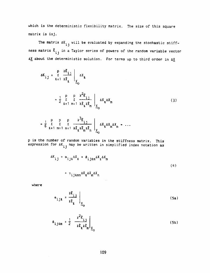
which is the deterministic flexibility matrix. The size of this square

matrix is ixJ.

The matrix 6Kij will be evaluated by expanding the stochastic stiff-

ness matrix _ij in a Taylor series of powers of the random variable vector

&X about the deterministic solution. For terms up to third order in AX

aKij = Z0: I a_z

AX

X--O

,p÷ _ E E

_:I m:1 aX a_mAXzAX m

X-o

(3)

1 P P P g3Rij I

m=1 m=1 n=1 aRmaRmaR n x

p is the number of random variables in the stiffness matrix. This

expression for AKij may be written in simplified index notation as

where

AKij = =ij_aX£ + Bij_m_XzAX m

÷ YijtmnAXzAXmAX n

aR [___!/

aiJ_ - @_£ X

--o

(_)

(5a)

I

sij_m - 2_2_£_

aX_.aXm x-.o

(5b)

109

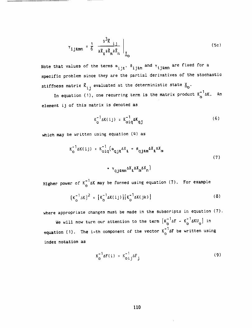
1 a3_ il

YijSmn : 6"a_sa_maE n x

--0

(5c)

Note that values of the terms sij_' Sij_m and YiJ_mn are fixed for a

specific problem since they are the partial derivatives of the stochastic

stiffness matrix _iJ evaluated at the deterministic state -oX.

In equation (I), one recurring term is the matrix product K-I&K.0

element ij of this matrix is denoted as

An

which may be written using equation (4) as

-I + BqjzmAX AXKSI_K(ij) : Koiq(_qj_&X£ m

+ Yqj_mnaX_aXmaXn )

Higher power of KSIAK may be formed using equation (7).

[KoI_K)2 : [KoIAK(ij)I[KSIAK(jk) ]

For example

(7)

(8)

where appropriate changes must be made in the subscripts in equation (7).

We will now turn our attention to the term [KoI F- Ko AKUo] in

equation (I). The i-th component of the vector KSIAF be written using

index notation as

K-IAF(£)o : K'1oijaFj (9)

110

Likewise, the i-_h component oF the vector KoIAKUo becomes

m

Ko1_ZUo(i): K_q_KqjUo_

-I= K (= aX + _maX_aXm (10)oiq qJ_ L Bqj

÷ YqJ_mnaX_aXmAXn)Uoj

The expression [K'lar - K-IAKUo ] was denoted in equation (17) [Ref 1]0 0

as the vector AU I. Its i-th component may be written using equations (9)

and (10) as

_u_(i) =_[Kol_r- Kol_K%!

-1 1= KoijaF J - KoiqlaqjcaX ¢ + SqJCmaXiaX m

(11)

+ YqjLmnaXlaXmaXn)Uoj

we will call equation (11), the first order term in K_ I,because it

only involves linear terms in this matrix. Likewise, from equation (I),

the second order term in K"1 for the vector component AU2(i) may be0

written as

_u2(i) : -(Z_I,_K)IIK_I,r- Kol_,KUol

: -K-IAK(IJ)AUI(J)0

-1: -Koiq(:qj_aX ¢ + SqjLmaXtaXm

*YqJLmnaXtAXmAXn)AUI(J )

(12)

*Note: The subscript o always represents the deterministic state. It

does not represent an index oF summation.

111

AUI(j) is evaluated from equation (11) with the appropriate subscript

change of j for i.

The total stochastic displacement vector 0 is the sum of the terms

+ aU ÷ aU 2 + 6U 3 ÷ (13)0 = U° I "'"

where the following recursive relationship exists

where _ui =I (K-oi_F- K'oi_KUo1

_% = -(KoI_KI_uI(14)

_ui = -IKo1_Kl_ui_I

The next part of the discussion presents an approach as to how the

stochastic strains and stresses may be computed from the stochastic

displacement vector. In general the element strains are computed from the

global displacement vector and the strain-displacement matrix. If _(s)

represents the strain vector in element s, then

_(s) : _(s) 0 (15)

where _(s) is the element strain-displacement matrix.

if randomness can enter in the structural geometry.

_(s) is stochastic

We will take

_(s) : B(s) ÷ aB(S) (16)0

f _where B_s' is the deterministic strain-displacement matrix. It seems

O

consistent with the method of computing AK [see equation (3)] to evaluate

AB (s) by expanding _(s) in a Taylor series about the deterministic state.

i12

This gives

=(s)

r_

%'1 a_L

1 p P

ax_÷_ _L=l m=l

X.-o

1

_.L_2"(s)

I AXLAXmaX_Xm X

-o

a3 (s)IP P P iJ

E E AXLAXmAX n

[=I m=1 n=1 aX[aXmaX n x-o

In terms of index notation,

(17)

-(s) _ax_aBij = aij + 8ij_maXtaX m + YijLmnaXLaXmaXn(18)

where the _, 8 and T are the partial derivatives of _(s)ij evaluated at

Therefore, s, 8, and _ are entirely deterministic.X .-o

In a similar manner, the strains can be related to the stresses. For

no initial stresses, the relationship between the stress and strain vector

in element s is

?(s) = C(s)[(s) (19)

where C (s) is the elasticity matrix. Since C (s) is generally stochastic

C(s) = C(s) + aC(s) (20)o

where C (s) is the deterministic elasticity matrix. As in the calculationo

of AK and &B (s) , the AC (s) matrix will be computed by expanding C (s) in a

Taylor series about the deterministic solution. Thus

ac(S) = - =iJ = _ijzAX_ ÷ BiJLmAXLAXm + YijLmnAX_AXm6Xn

+ ... (21)

113

where _, _ and _ are the partial derivatives of _(s) evaluated at X andiJ -o

are entirely deterministic. Obviously a relationship exists between the

matrices aKij' aB(S)ijand _c!S)ljdepending on the nature of the stochastic

state vector X .-o

Using the equations developed in this section, expressions are now

available for the computation of the structure's random displacements 0,

element strains _(s) and stresses T(s) entirely in terms of the random

load vector ag and the vector _X of the random variables in the stiffness

matrix. Obviously, the amount of computational effort depends on how many

terms are retained in equation (13) and to what order are powers of 5X

retained in AK [equation (3)], aB(s) [equation (18)] and AC (s) [equation

(2_)].

2.0 Truncation of Stochastic Displacement Vector in Terms of Powers-I

of K..___o..

Equation (13) expressed the total random displacement vector as

0 = U0 ÷ &U1 ÷ &U2 + &U3 + ... (22)

-I

where AU i involves the i-th power of the deterministic matrix Ko

Successive terms for AU i are related by the factor KoIAK. As shown by

equation (14)

i = -CKol } ui_l (23)

Ko 1From the magnitudes of and AK encountered in engineering

problems, it is expected that AUi will be small compared to AUi. I. Thus,

114

at this stage of the Formulation, it seems reasonable to take only the

first two terms to approximate O, L.e.,

+ aU (24)0 U° I

where AU1 is given by equation (11).

3.0 Truncation of Power Series Expansions for AK t AB_ and &C

The expressions For AK, AB (s) and AC (s) were developed in terms of a

Taylor series about the deterministic state. These are given up to terms

of third order by equations (4), (18) and (21). The coefficients of the

powers of aX must be evaluated by taking the partial derivatives of the

sti/fness, strain-displacement, and elasticity matrices.

For the present time we will confine the analysis by retaining only

the linear terms in AX. This is a reasonable assumption if the variances

oF the random variables in the stiffness matrix remain small. Hence only

compution oF the /irst, and not the higher partial derivatives oF the R,

_(s) and C(s) matrices is required. Under this assumption equations (4),

(18) and (21) reduce to

aKij : _ij_aX_

(S)aBij : =ijzaX L (25)

(s) :aCij : =ijlaXt

115

4.0 SLm_nary of Structural Response Equations

Under the assumptions made in the previous two sections, the

dependent stochastic displacement, strain, and stress vectors may be

expressed as

;(s) = jR(S) -i =-oiJ ÷ =LJcaXz]OJ (26b)

• c(S) =ijzAXz ] _s)F(s)_ = [ oij ÷ = ; (26c)

In terms of the random variables Ag and AX , the strain and stresses

may be finally expressed as

¢(i = '-oiJ ÷ _ij oJnAFn K q=qnrUon r

1= lc(s) = ]• oip + =ipLAXz

=(s) 1+ =pmaXm!j "Qopj

+ K-1 -1 &X ][Uoj oJnaFn - KoJqaqnrUon r

(28)

Equations (26a), (27) and (28) formulate the global stochastic

structural and element response entirely in terms of the random loads and

variables in the stiffness matrix. Note that the displacement vector 0 is

linear in the random variables, while the strains and stresses contain

terms up to quadratic and cubic in &F and AX , respectively.

116

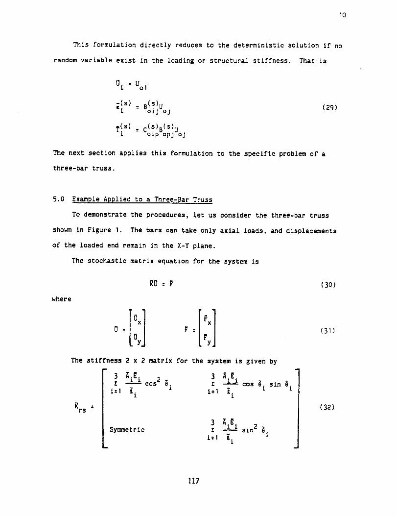
I0

This formulation directly reduces to the deterministic solution if no

random variable exist in the loading or structural stiffness. That is

0 i = Uol

;(s) = B(S)ui oi] o] (29)

?(s) = c(s)B(S)U£ dip opj oJ

The next section applies this formulation to the specific problem of a

three-bar truss.

5.0 Example Applied to a Three-Bar Truss

To demonstrate the procedures, let us consider the three-bar truss

shown in Figure I. The bars can take only axial loads, and displacements

of the loaded end remain in the X-Y plane.

The stochastic matrix equation for the system is

R0 = _ (30)

where

I0= t=

0y ty

The stiffness 2 x 2 matrix for the system is given bym

3 _.S 3 _._.__.._ cos 2 _ _ i_._._Icos _ sin _

i:I _i Z i=I _i l Z

rs

3 _i_iSymmetric _ -- sin 2 _.

i:1 E.1

/

(32)

117

In the general stochastic finite element problem the cross-sectional

areas (_i), modulii of elasticity (_i), bars' lengths (_i) and load vector

_, may all be considered random. However, the bars' lengths (_i) and the

angles (el) (see Figure I) must satisfy geometric compatibility conditions

even though they are random.

In this example, we will somewhat simplify the problem by considering

that in the undeformed state, the truss is geometrically symmetric. Thus

el = -e3 : _

§2 : 0

(33)

The lengths of the bars may be random. However, the lengths of bar I

and 3 are related to the length of bar 2 by the compatibility relationship

(3_)

The length of bar 2 (denoted now as { ) can also be expressed in

terms of the fixed distance d and the angle e as

: d cot _ (35)

The stiffness matrix may now be expressed as a function of the seven

random variables _i' _i' and

rs

_2

(_1E1 * _3_3 ) (i2 ÷ d2) 3/2

_2£2

Symmetric(i2 ÷ d2) 312

(36)

118

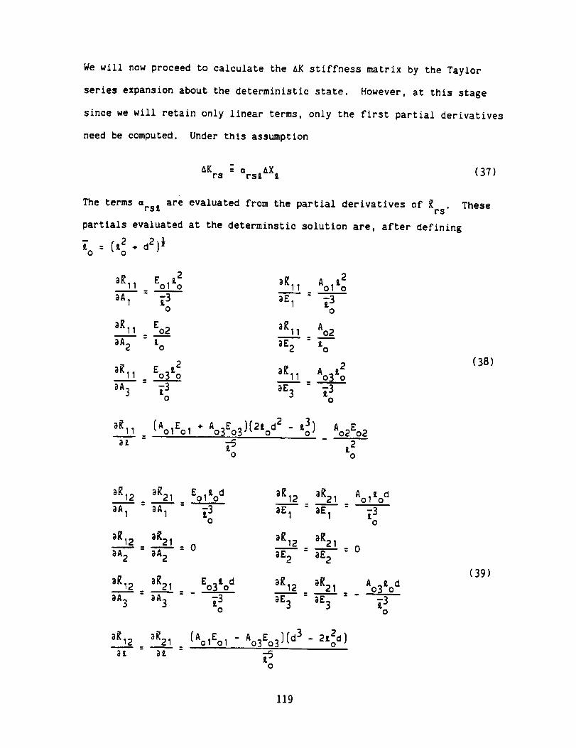
We will now proceed to calculate the &K stiffness matrix by the Taylor

series expansion about the deterministic state. However, at this stage

since we will retain only linear terms, only the first partial derivatives

need be computed. Under this assua_p_ion

AKrs arszAX i (37)

The terms Qrsl are evaluated from the partial derivatives of Rrs" These

partials evaluated at the determinstic solution are, after defining

t2t2 _11 Aol o_11 Eol o

aAI " _3 _EI [3O O

a_11 Eo2 a£11 Ao2

aA2 " _o a£2 Zo

a£1_._.! = Eo_o a£11 Ao3Zo2

aA3 [3 a£ 3 [3O O

(38)

a_11 (AolEol + Ao3Eo3)[21od2 - L_} Ao2Eo2

a_ _-_ Z2o 0

a£12 a_21 EolZod

aA 1 " aA1 E3O

a£12 aR21

aE 1 aE 1

AolZod

a£12 aR21

aA2 " aA2= 0

ag12 aR21

aE2 - aE2= 0

aR12 a_21 Eo31od a_12

aA3 aA3 [3 aE3O

aR21 = . Ao3_od

- aE3 E3O

12a_

aR21 (Aoi£oi - Ao3Eo3}(d3 - 2L_d)

(39)

119

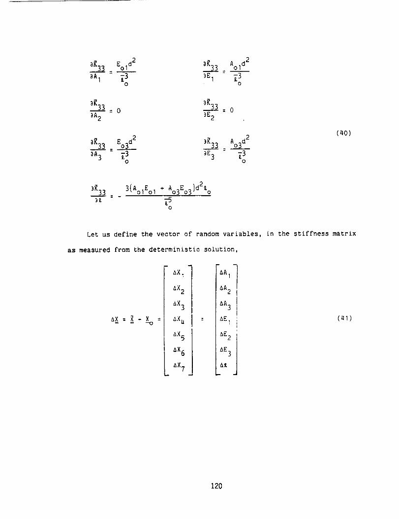
a_33 Eold2 a£33 Aold2

_EI _30

a_33 Eo3d2

aA3 - [30

3_33 _ Ao3d2

aE3 - _30

(40)

)_33 3[AolEol + Ao3Eo3 )d2zo= --

0

Let us define the vector of random variables, in the stiffness matrix

as measured from the deterministic solution,

aX:_-X

AX.

aX2

aX3

aXa

a×5

L a×ax7

o

AAI

AA2

aa 3

: AE,1

(al)

120

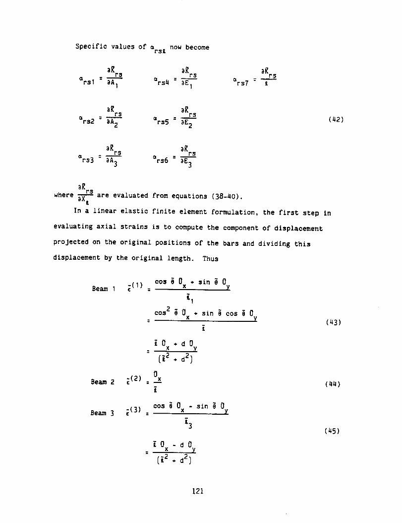
Specific values of ars _ now become

_ aRrs rs

_rsl = _A--_'- =rsg - aE1

_Rrs

rS rs

=rs2 - _A2 =rs5 - aE2(q2)

aR _rs rs

=rs3 - aA3 =rs6 =

aRrs

where a--_-are evaluated from equations (38-40).=b

In a linear elastic finite element formulation, the first step in

evaluating axial strains is to compute the component of displacement

projected on the original positions of the bars and dividing this

displacement by the original length. Thus

Be== 1 ;(1) =

Beam 2

Beam 3

cos _ 0 + sin _ 0x y

I

cos 2 _ 0 + sin _ cos _ 0x y

_0 +dOx y

- (i2 + d2]

0;(2) x

;.(3)cos _ 0 - sin _ 0

x y

_3

_0 -dOx y

• d2]

(43)

(44)

(aS)

121

The strain displacement matrix _ relates the element strains to the

nodal displacements.

-(s) _(s) 0 (_6)¢

In this case

§(s)

n)

E

[2 .,- d2

1

[

E

[2 + d2D

m

d

[2 . d2

D d

[2 + d2w

In previous discussions the stochastic _(s) was separated into

deterministic and stochastic parts

(47)

§(s) _(s) + aS(s)= UO

(U8)

The deterministic part B(s) can be evaluated by substituting io for0

[ in equation (qT). _B(s) can be computed by expanding _(s) in a Taylor

series about Lo. To the first order terms in 51(&X7) this gives

m

AS(s) = -

-{d2 _ ,o2} x

Lo

AX7

220

{d 2 - Z_}aX 7

0

21od_X 7

g0

0

29-odAX7

(29)

122

(s)In index notation ABij was expressed for element s as

-(s) -ABij = _ij£AX_

a u

sijZ can be evaluated from expression (49). Thus aij £

ijl except

(50)

= O for all

m

s117 : _317

2Z d_ 0

a127 : - _317 - _4 (51)o

o

To complete the calculation of the dependent random variables, the

expressions for the stochastic stresses must be derived. In general,

stresses are calculated from

-(s) c(s) (s)o : _ (52)

where _(s)is the elasticity matrix. For the three-bar truss problem, the

_(s) matrix only involves the modulus of elasticity. Thus, following the

usual notation

_:C +AC:o

J

Eol

0

0 0

Eo2 0

O O £o3

aE

+ 0

0

01

AE2

0

0

aE 3

(53)

The Taylor series expansion about the deterministic state only yields

terms to first order since the elasticity matrix is linear in modulus.

123

In index notation 8C is

where 8Xq = 8E 1

8X5 = _E2

_X6 = aE3

=

This gives for QIJ&

-(s) :

8Cij = QijzSXz (54)

= 0 for all iJZ except (55)=ij&

_11tI : &225 = &336 : 1

This completes the formulation for all quantities used in equations

(26a), (27) and (28) for calculation of the stochastic displacements,

strains, and stresses. The next issue concerns what probabilistic methods

can be employed to evaluate the probabillstlc response of the system.

In closing, a few comments on the question of geometric compatibility

are in order. In this problem, the general stiffness matrix [equation

(32)] is given in terms of the angles ei and lengths Ei. The angles Bi

were eliminated in the formulation through compatibility conditions, and

the final results only contained the random variable a&(AX7). An

alternate approach is to retain the random variables aei and _ti in the

formulation of 0, _(s), and _(S)in equations (26a), (27) and (28). The

compatibility condition could then be imposed through the correlation

coefficients between the random variables for the probabilistic

evaluation.

124

Three-Bar Truss

FIGURE I

125

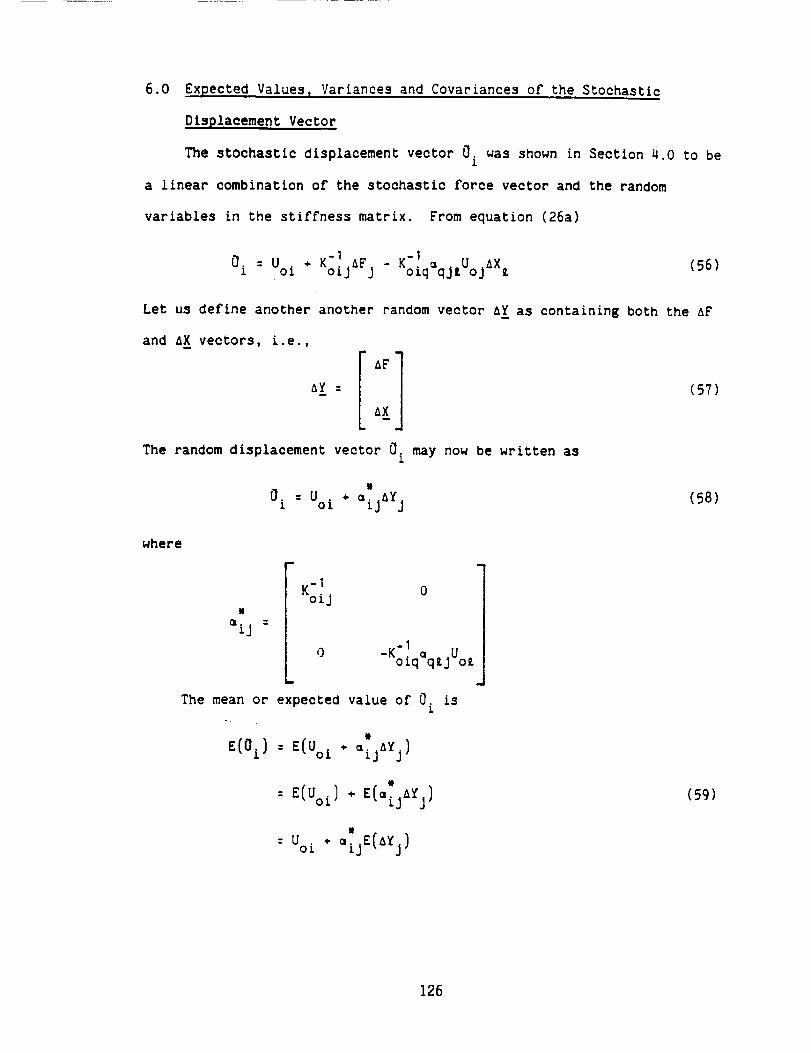
6.0 Expected Values t Variances and Covariances of the Stochastic

Displacement Vector

The stochastic displacement vector 0. was shown in Section 4.0 to be1

a linear combination of the stochastic force vector and the random

variables in the stiffness matrix. From equation (26a)

0 :Uoi + Ko:jaF j -Kol• " iq=qj LUoj aX _ (56)

Let us define another another random vector A[ as containing both the AF

and 6X vectors, i.e.,m

aY_: (57)

_x

The random displacement vector O. may now be written asi

I

0 L.: Uoi + =ijAyj (58)

where

N

I

Koi j 0

-1

0 -K ° iq=q_jUo_

m

The mean or expected value of O. is1

t

E{Oi) : E(Uoi * aijaY J)

: E{Uoi) ÷ E[(*ijaYj)

m

• * =[jE(aYj): Uol

(59)

126

The variance of O. isI

v(0i)= E{[0_- E(0i)]2}

= E(0_2)- [E(0i)I2

(60)

which for equation (58) reduces to

n

v[Oi) : }"(c,£j)2 V(AYj)j=l

÷

n n

_ _[j=ik Cov(aYj, aYk)j:1 k=1

(61)

The covariance term Cov(aYjaYk) , denoted as _Jk' is defined as

Cov(AYjAYk) = E[{AYj - E(AYj)}{Ay k - £(Ayk)}]

= E(AYjAYk) - EIAYj)E(AYk)

If the random variables in A_yare independent, then they are

uncorrelated and

(62)

Cov(aYj, aYk) : Ojk : 0 (63)

In this ease, the variance of 0[ becomes simply

n" 2

V(0 i) : _ I_[j) V(aYj)j:1

(64)

The correlation coefficient will not be zero in the general case and

must be evaluated. Figure 2 illustrates how correlation could occur

within each set of random vectors AF and AX and even between AF and 8Xm m

127

7.0 Higher Moments and the Distribution of 0i for Independent RandomVariables

The special case of independent, i.e., uncorrelated random variables

permits a relatively simple calculation for the higher-order moments of

the stochastic variable 0 i. Hines and Montgomery [2]* show that if

MAyj(t) is the moment generating function of AYj, then the moment

generating function of 0i for equation (58) is

U .t

M (t) : e oi {MAY1{a£1t).MAY21ai2t) ... MAYnla nt)}O.i

(65)

Recall that the moment generating function for the random variable Z is

defined as

MZ(t) : E{e tZ) (66)

and has the property

drMz(t)- E(zre tz) (67)

dt r

Thus

E(zr) _ drMz(t)dt r

t:O

(68)

From knowledge of the type distributions of the independent random

variables in A[, we know their moment generating functions. From equation

(65), the moment generating function for O. can be constructed, and the1

r-th moment is

mr

d r: E(0r) :--M (t)

i dtr O.i t:O

(69)

[2]* Probability of Statistics in Engineering Management and Science,Wiley, 1980.

128

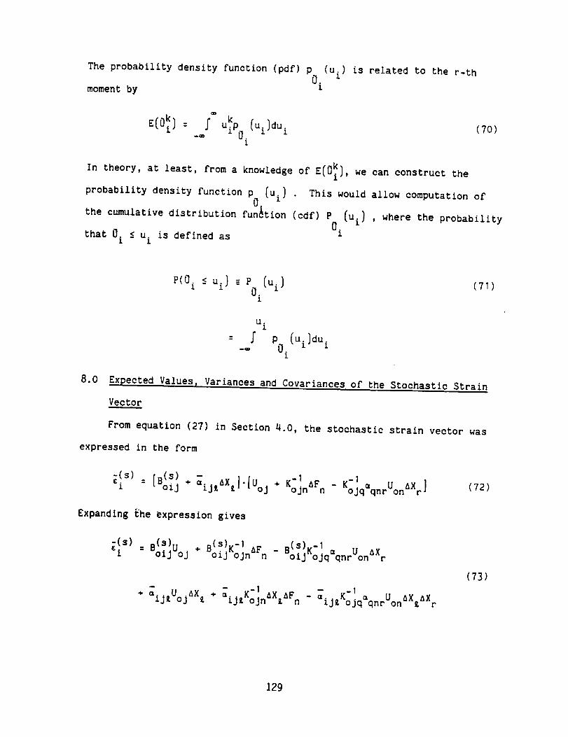
The probability density function (pdf) pO.

moment by I

(ui) is related to the r-th

k )duiE(0 ): ..F uip0.("i1

(70)

In theory, at least, from a knowledge of E{0_), we can construct the

probability density function PO [ui) " This would allow computation of

the cumulative distribution function (cdf) P (ui) , where the probabilityO.

that O. _ u. is defined as i1 l

P(0. < u ) _ P Cui) (71)i- i O.

I

ui

] P (ui]du i

-® 0i

8.0 Expected Values r Variance s and Covariances of the Stochastic Strain

Vector

From equation (27) in Section 4.0, the stochastic strain vector was

expressed in the form

¢i oiJ ÷ aij_ax_l'[Uoj naFn - KoJq=qnrUon r

Expanding _he expression gives

_s) : s(S)u + B(s)K-] .(s).-1oiJ oj oiJ-ojnaFn - SoijKojqSqnrUonaXr

+- *- o_ - _ . K'I = U aX AX=ij_UojAX_ _ij_ K naX_aFn ij_ ojq qnr on 9. r

(73)

129

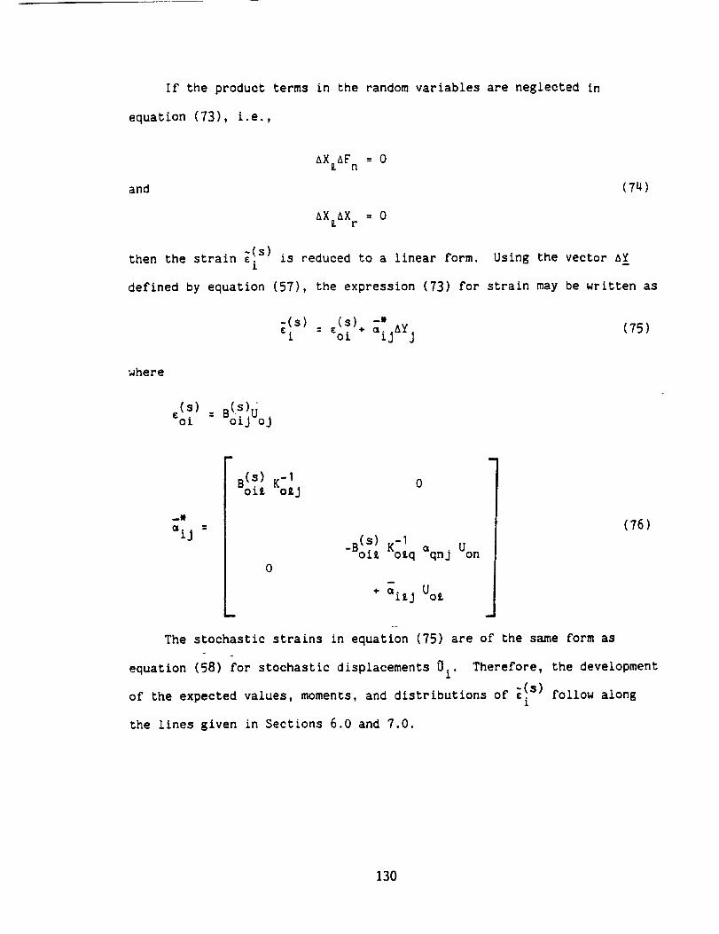
If the product terms in the randomvariables are neglected in

equation (73), i.e.,

_X_AF n = 0

and

AX_X r = 0

then the strain -(_¢'s'.l

is reduced to a linear form. Using the vector AY

defined by equation (57), the expression (73) for strain may be written as

--U

;!s)_ : (.S)÷ol =ij_Yj (75)

where

_(s) : B(s)Uoi oij o]

a(s) -Ioi_ Ko_j 0

_(s) K-I-Boi_ otq Sqnj Uon

0

+ ai_ j UoZ

The stochastic strains in equation (75) are of the same form as

(76)

equation (58) for stochastic displacements 0i. Therefore, the development

-(s)of the expected values, moments, and distributions of ¢i follow alone

the lines given in Sections 6.0 and 7.0.

130

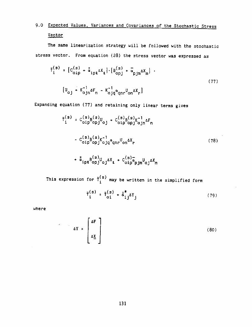
9.0 Expected Values r Variances and Covariances of the Stochastic Stress

Vector

The same linearization strategy will be followed with the stochastic

stress vector. From equation (28) the stress vector was expressed as

[c(S = I'[B(s) - li oip + _ip_AX_ opj + =pjmAXm

K-I -I[Uoj ojn_F - K _x ]n ojq=qnrUon r

(77)

Expanding equation (77) and retaining only linear terms gives

_(s) : c(s)B(s)u . c(s)B(S)K_1i oip opJ oJ oip opj ojnaFn

- c(S)B(S)K'I : uoip opj oJq qnr-onaXr (78)

+ _ B(s!U .AX + c(s)_ U aXipl opj oj _ oip pJm oj m

where

This expression for _(s). may be written in the simplified formI

_(s)z. : _(S)oi÷ _:jAYj (79)

aY : (80)

ax

131

T(s) = c(s)B(S) uoi oip opJ oj

-ICoipBopg.Kog.J

0

0

_(s)- -1- CoipBop_Kozq:qnjUon

+ C(S)_ Uoip p_j o_

: _(s).+ _ipjOop_oZ

(81)

The linear form of equation (79) allows the same development for

expected values, moments, and distributions of _!s) as for 0. and _(s). int I t

Sections 6.0 thru 8.0.

10.0 Comments on Implications of Linear Formulation

In the previous sections the dependent stochastic variables in

displacement, strain, and stress were cast in the linear format

--N

• +_ &YOi : 0o_ ij j

-(s) _(s) -"• : . + a. aY (82)c ol 1j j

First, such a format has several nice properties in the evaluation of

the probabilistic response. If the elements of the random variable vector

a[ are each normal and independent, then the random variables vectors

o!S!l -(s)¢iand _!s)l are normal. Furthermore, if the elements of AYj are

independent, then o(s)., _(s). and _!s) approach normal distributions as

the size of the aY vector, i.e., dimension J, becomes large. This is

irrespective of the type of distributions in the a_ vector.

132

TEKPEKATUKE LOAD

2

\1

F n

o

o

o

Correlation Between Material Properties

as a Function of Locatlon

Correlation Between Applled Forces

Correlation Between Material Properties and

Appl£ed Loads, e.g., Temperature Dependent

Properties

FIGURE 2. EXAMPLES OF CORRELATION BETWEEN RANDOM VARIABLES

133

Section 4

A Preliminary Plan for Validation of the First Year PFEM Code

Dr. Y.-T. Wu

Dr. O.H. Burnside

Southwest Research Institute

September 1985

134

General Description

This plan describes test cases designed to validate the first-year

edition of the PSAM PFEM computer code which has the following capabilities:

Ii The code combines the conventional finite element method using the newly

developed perturbation scheme for generating analytical performance

function, with the fast probability integration (FPI) algorithm. The

performance functions will consider all important design-related

variables such as the displacements, strains, stresses, natural

frequencies, limit states, etc.

. The code employs complex elements (beams, plane stress/strain,axisymmetric, plates, and shells), linear elastic material behavior, andsmall deformations.

. For static problems, the loading vector can be treated as a correlated

random vector. For dynamic problems, the steady-state random responses

of a linear stochastic structure to stationary random loading can besolved.

. The output of the code, for probablllstlc design purposes, include the

probability density functions (pdf) and the cumulative distribution

functions (cdf) of the performance functions, and the probability of

exceedence or the reliability of the response variables.

The following cases were carefully selected to test the many features of

the PFEM code. Most of the cases are considered well-deflned, wlth specifiednumerical design values and distributional information. However, there are

some cases where only exact or good approximating performance function aregiven. Those are the cases where some trial and error procedures must be done

to generate meaningful input data. A case for testing probablllstlc shell

response has not been finalized yet due to the difficulty of finding a "good"performance function for checking purposes. A test case involving a twisted

cantilevered plate (relating closely to the turbine blade in the PSAM project)

may be included in the validation, depending on the availability of theaccurate theoretical solution of the natural frequencies.

In summary, the primary purpose of this test plan is to define the scope

of the PFEM code validation. All test cases, In their final version, will be

given an "exact" performance function, so that the advanced reliability

analysis methods, as well as Monte Carlo simulations, can be applied for the

comparisons. The test cases will, in general, fall within the above-deflned

capabilities of the PFEM code, and will cover all important aspects of the

probabilistlc design.

Test Cases

Case I. Cantilever Beam (Solution is given in Section 4 Appendix)

The cantilever beam modeled in Figure I is subjected to static loadlngs,

Pi(i-1,5). Pl'S are correlated with the correlation coefficient defined as:

135

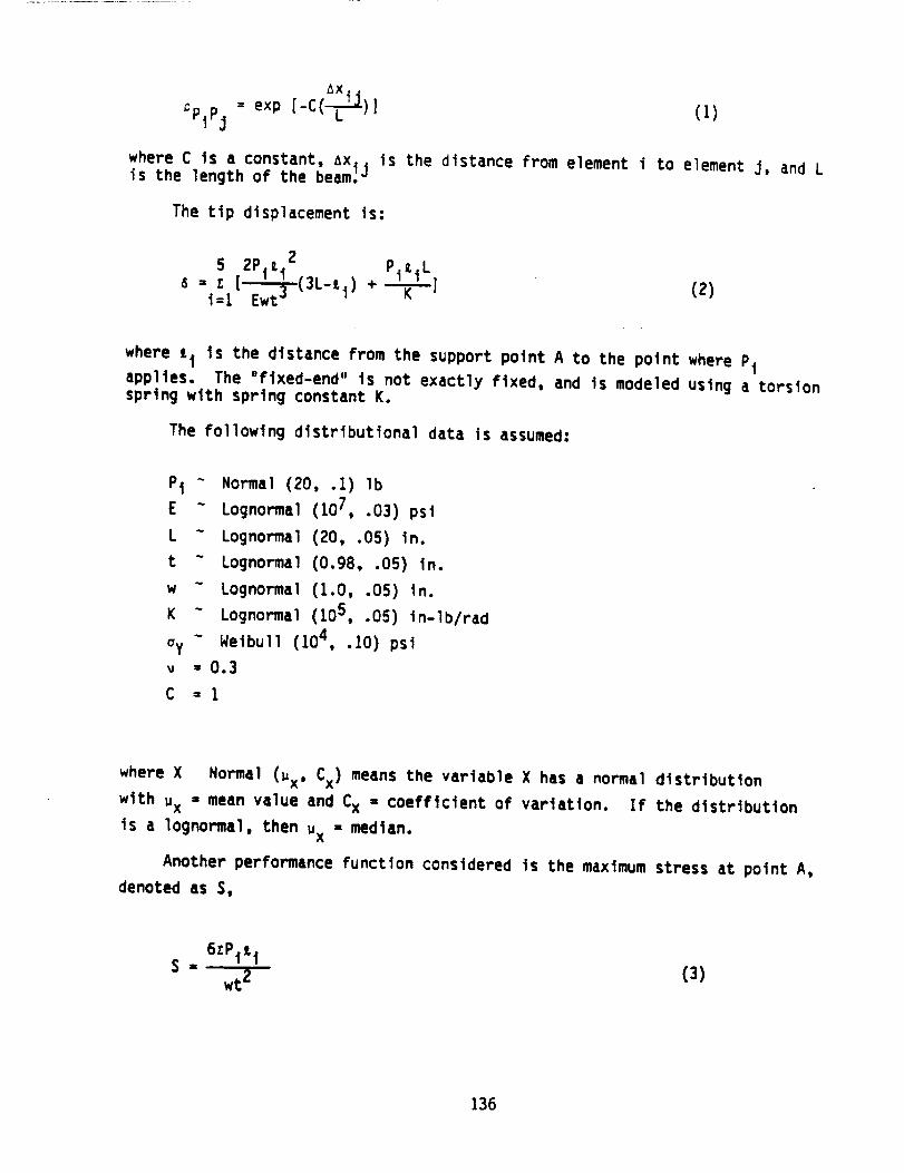
_X, °

= exp [-C(L--_)] (I)_PIPj

where C is a constant, axl4 is the distance from element i to element J, and Lis the length of the beam. _

The tip displacement is:

5 2Pi0i2 Pi¢i L

6 = z;i_i[Ew-_t (3L-_i) +

(z)

where iI is the distance from the support point A to the point where Pl

applies. The "flxed-end" is not exactly fixed, and is modeled using a torsionspring wtth spring constant K.

The following distributional data is assumed:

PI ~

E ~

L "

t ~

W

K ~

ay

Normal (20, .i) Ib

Lognormal (107, .03) psi

Lognormal (20, .05) in.

Lognormal (0.98, .05) in.

Lognormal (1.0, .05) in.

Lognormal (105 , .05) in-lb/rad

Weibull (104 , .10) psi

where X Normal (Px' Cx) means the variable X has a normal distribution

with uX - mean value and CX - coefficient of variation. If the distribution

is a lognormal, then uX - median.

Another performance function considered is the maximum stress at point A,

denoted as S,

S ,, 6zPtLt (3)wt Z

136

The correlated loading vector, P, can be transformed to an uncorrelated

vector, _, using

E " ATP.. (4)

Where A Is an orthogonal matrix with column vectors equal to the eigenvectors

of the covarlance matrix, Cp;

L°nl - °nn_]

(S)

where

°iJ = Pij°i°J (6)

Using the inverse transformatlon of Eq. (4), the two performance

functions, namely 6 and S, may be written in terms of p , for example,

= {2(3L1._ - t._) t, iL T,T-lp8 ÷T} _-Ewt 3

(7)

where {-} Is a column vector. The mean and the standard deviation of p can be

computed as:

Up = ATup (8)

137

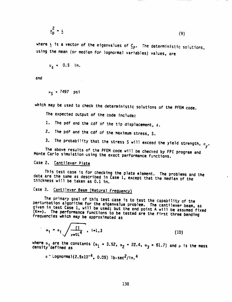
2

% = x (9)

where _ Is a vector of the eigenvalues of Cp. The deterministic solutions,

using the mean (or median for logno_al variables) values, are

u6 , 0.5 in.

and

uS = 7497 psi

which may be used to check the deterministic solutlons of the PFEM code.

The expected output of the code include:

I. The pdf and the cdf of the tip displacement, (.

2. The pdf and the cdf of the maximum stress, S.

3. The probability that the stress S will exceed the yield strength, _y.

The above results of the PFEM code wlll be checked by FPI program andMonte Carlo simulation using the exact performance functions.

Case 2. Cantilever Plate

This test case is for checking the plate element. The problems and thedata are the same as described In Case I, except that the median of thethickness will be taken as 0.1 in.

Case 3. Cantilever Beam (Natural Frequency)

The primary goal of thls test case Is to test the capability of the

perturbation algorithm for the elgenvalue problem. The cantilever beam, asgiven in test Case I, will be used; but the end point A will be assumed fixed

(K--). The performance functions to be tested are the first three bendingfrequencies which may be approximated as

_I " =I El , i-I,3 (Io)

where "4 are the constants (=I " 3.52, a2 - 22.4, a3 = 61.7) and _ is the massdensity'defined as

o ~ Lognormal(Z.SxlO -4, 0.05) lb-sec2/tn. 4

138

note that wi in Eq. (10) are the natural frequencies for the vibration motionparallel to yz-plane (see Figure I). To compute wi, for xy-plane motion, thethickness (t) and the width (w) need be switched in Eq. (10).

The values of w and t are chosen very closely in order to test the

capability of the code in identifying different modes which have approximatelythe same natural frequencies.

By substituting the mean or median values into Eq. (I0), the

deterministic solutions of _I can be obtained for checking the codesolutions. For example,

=I = 497.9 rad/sec, yz plane

= 508.1 rad/sec, xy plane

The expected output of the code is the cdf and the pdf of _I for bothdlrections.

Case 4. Rotatln 9 Beam (Centrifuqal Loadin 9 and Stress Stiffening Effects)

The geometry of the beam is given in Figure 2. The tip axialdisplacement due to centrifugal loading is:

(II)

where the variables are defined as:

Q - 2400 rad/sec

" Lognormal (g.Ox10 "4, 0.05) lb-sec2/In 4

L - Lognormal (3.844, 0.05) in.

E " Lognormal (2.9 x107, 0.1) psi

It can be shown that the tip displacement is also a lognormal variable whichcan be expressed by:

u(x-i) - Lognormal (6.77xi0 "3, 0.188) in.

Stress stiffening on the bending frequency can be included by using Galerkin'smethod Ill.

The performance function for the first bending frequency can beapproximated as

139

=V _-0371E12 + 2,886Q 2u °t 4

where the thickness t.is given as

(12)

t - Lognormal (0.0416, 0.05) in.

For the finite element model, the width, w, is given as

w - Lognormal (1.424, 0.05) in.

By substituting a value into Eq. (12) and letting

H = 1.0371Et 2 (13)=l 4

which has a lognormal distribution, Eq. (12) becomes

= = ^/H + 1.662 x I07' (14)

Using Eq. (14), the cdf of w,F=(=), can be expressed in terms of the cdf of H,

FH(h ). Because H is a lognormal variable, it can be shown that

F=(=o) = FH(=o2-1.662 x tO/)

ln(wo2-t.662x107)-UtnH)= ®H(

_tnH

(15)

where OH(- ) is the standard normal cdf. Therefore, an exact distribution

function of _ can be computed easily.

The PFEM code will be expected to generate pdf and cdf for the tip axialdisplacement and the first bending frequency. The results will be compared

with the exact lognormal distributions.

Case B. Rotating Beam - Plate Element

Repeat Case 4 using plate element.

140

Case6. Twisted Cantilevered Plate

A twisted plate is shown in Figure 3 where a rectangular plate of length

a, width b and thickness h is shown clamped at one edge, with the opposite

edge pretwisted through an angle ®.

Although much more complicated, turbine blade is basically a twisted

plate and, therefore, the model shown in Figure 3 would be a good validation

test case. However, the vibration of rotating blade, even for the relatively

simple configuration considered, have Found to be very dlfficult to analyze bytheoretical methods. Widespread disagreement has been found among published

results, especially when the aspect ratio (a/b) is relatively small, e.g., oneor two.

To clarify the problem, a Joint industry/government/university NASA-Lewisresearch effort was initiated to obtain comprehensive theoretical and

experimental results [ZI. All of the theoretical methods used were found to

be either Inappllcable or unreliable for certain ranges of the geometric

parameters (a/b, b/h, ®).

For a valldation test to be meaningful, it is essential that the

performance function be accurate. For this reason, this test case will beincluded only if a suitable performance function can be determined.

Case 7. Plate with Different Correlated Loadlngs in Oifferent Zones

The plate model considered here has a geometry shown in Figure 4 and is

simply supported. The plate is separated into four zones with each zone

having a different correlated static loading.

The performance function considered is the center (point c)

displacement 6 which, for a single point loading P, has the followingtheoretical expression.

li ]" 4_2P i (m2+ n2)2 sin _-_ sin-_--_ (16)_ Inl

For simplicity, define F as a factor representing the series within thebrackets in Eq. (IB), i.e.,

where

nL2

--_DPF (17)

D - Et3

12(i. 2) (18)

141

For n loads, _ is

4tZ n

6 " _ 1"-1z (PF)I (19)

Now consider a total of slxty-four loads as illustrated in Figure 4. Theloads will be divided into four zones. In each zone the loading vector will

be denoted by PI" For example, at zone I (i-1,4),

Pi" (20)

The loads in each zone are correlated with the correlation coefficients

defined in each zone as

I ll°1.1,]el " (zz)

P16,1 " " °16,16 i

The elements oij in the above matrix are defined as

olj = exp(-K ax j + ay j ](22)

where ax and Ay are x-dlrection and y-dlrectlon distances, respectively.

Using Eq. (22), a covarlance matrix, _I' can be established to subsequently

generate a transformation matrix, _I' such that

_i " AIT-PI (23)

where _I is the uncorrelated 1oadlng vector at zone I.

Using Eq. (23), the middle displacement can be formulated as

4Lz 4 E(AT-it-1(24)

which will be used as a comparison basis.

142

Becauseof the large amount of random variables involved, the selectionsof the material properties, as well as the loads and correlation coefficients

in the four zones, have not been completed yet. However, the list of the

random variables and the deterministic parameters are given as follows:

Random Variables: E, t, v , ¢, P1 to P64

Deterministic Variables: KI to K4

The goal of the analysis is to construct the distribution of 4.

Case 8. Shell Element

Due to the difficulties of selecting a proper performance function for

reliability analysis, thts case (employing shell elements) has not beendetermined.

Case 9. Random Vibration [3]

The case chosen is a simply supported beam under concentrated randomforce F(t) as shown in Figure 5. F(t) is a random function of time,

representing band-llmited white noise with cutoff frequency _c:

E[F(t)] - 0

o, I'l- 'c$F (u_) " Z0, otherwise

where E[.] denotes the mean value, SF is the spectral density.

The displacement is a stationary random process which can be formulatedas:

. I ®6(x,t) _ _ v_-Z_((x) [" hj(T)dT [lq((,t-T)$j({)d{

j-I J J -- o

(ZS)

g

q(x,t) - z qj(t)$j(x) (26)J-I

. 1

qj(t) - vjz J" q(x,t)_j(x)dx, v_ - ]'l,2(x)dx (27)o o J

143

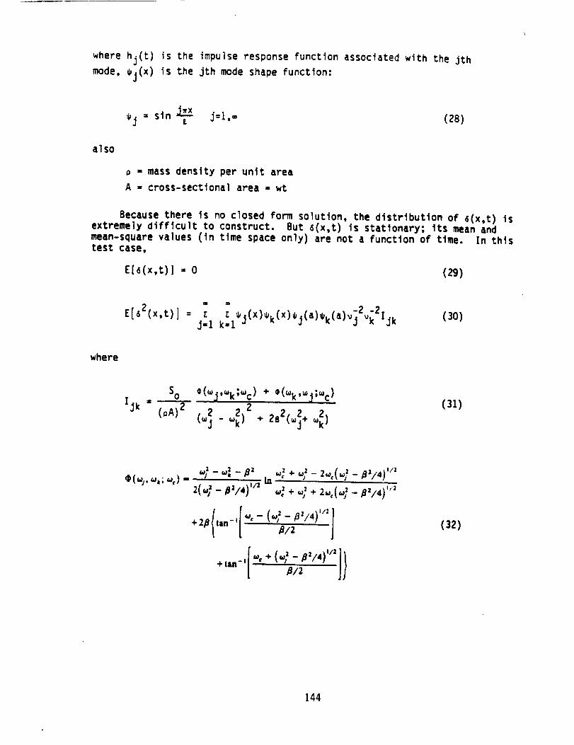
where hi(t) is the impulse response Function associated with the jth

mode, _j(x) is the jth mode shape function:

_j = sin J_xL j=l,- (28)

also

= mass density per unit area

A - cross-sectional area = wt

Because there is no closed form solution, the distribution of 6(x,t) isextremely difficult to construct. But _(x,t) is stationary; its mean and

mean-square values (in time space only) are not a function of time. In thistest case,

E[6(x,t)J= 0 (29)

: z _l_j(X)_k(X)ej(a)ek(a)v]2Vk21jk (30)E[a2(x't)i j-1 k-

where

so ®(_j,_k;_c) + .(_k,_j;_c)

2z 2s2( ÷ (3z)

<4- ,,,i- _' ,,,':'..'+W- z<.,.(,.,i- _'/4j"'2(,4- p'/,,)'' _:+W+2,=.(<,,_- a,14)'"'

(32)

144

a = 2¢jwj = c/_A (33)

where c is the damping coefficient and cj is the damping factor of the jthmode.

The goal of the reliability analysis is to construct, at x-a, thedistribution of the mean-square value defined In Eq. (30). (This distribution

may be used to establish the distribution of (, considering all randomvariables).

The cutoff frequency Wc will be chosen such that

_14 < _C

where _14 is the mean value of the 14th natural frequency. Following is the

llst of the random variables and the deterministic parameters:

Random Variables: E, w, t, L, c, o

Deterministic Value: a, So, wc

Based on the chosen mean or median values, the following nondlmenslonal

parameters will be chosen:

H - - 0.01

Qc = '"c_/(E/_)I/2 = 2_

B = BL/(E/o) I/2 = 0.02

an=-=0.3

t

References

I. PSAM Proposal, Technical proposal, Part 2, Appendix C.11.

e Lelssa, A.W., Macbain, J.C. and Klelb, R.E., "Vibrations of Twisted

Cantilevered Plates - Summary of Previous and Current Studies," submitted

for publication In Journal of Sound and Vibration.

o Ellshakoff, I., Probablllstlc Methods in the Theory of Structures, JohnWiley, & Sons, Inc., 1983.

145

Modeled Using a Torsion Spring

P1

2

P5

X Y

FIGURE I. Mode] Definition of a Cantilever Beam

146

Axis of

Rotation'_r "!

I!!

Z

FIGURE 2. Rotating Beam Geometry

147

Dots RepresentingLoading Points

Y

X

t:.05"

Y

0

P3' P3

I

P2' P2

P4' P4

FIGURE 4. The Plate Model for Test Case 7

148

\\\\

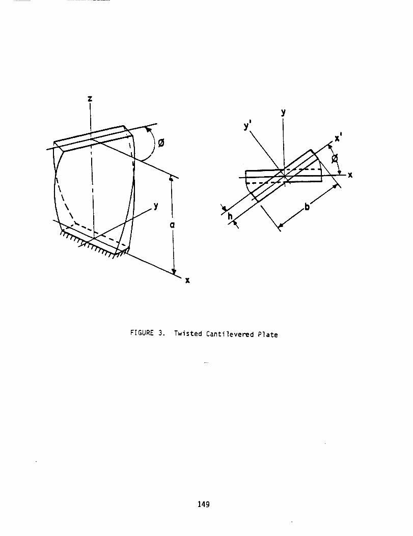
Z

X

X

FIGURE 3. Twisted Cantilevered Plate

149

_I F(t)

6(a,t)

£_IrI

L

SF(_)

C_u(rad/sec)

FIGURE 5. Simply Supported Beam Under ConcentratedRandom Force F(t)

150

Section 4 Appendix

Validation Case for the First Year PFEMCode

Dr. Y.-T. WuSouthwest Research Institute

November1985

151

Introduction

A preliminary plan for validation of the first year PFEM code was

described earlier in the PSAM Monthly Progress Report No. FY '85-12

(Attachment 4). Presented herein is the solution to the validation testCase 1.

Case I

Problem: The cantilever beam modeled in Figure I is subjected to static

loadings, Pi(i=l,5). Pi's are correlated with the correlation coefficientsdefined as:

_X I

_PiPj = exp [-(---_L)](1)

where axi is the distance from element i to element j, and L is the length ofthe beam. j The goal of the analysis is to determine:

I. The cdf (cumulative distribution function) and the pdf (probabilitydensity function) of the tip displacement, 8.

2. The cdf and the pdf of the maximum stress, S, at point A.

.

Solution:

The probability that the stress S will exceed the yield

strength, Oy.

The covariance matrix of the correlated static loadings is

I e-'2 e-'4 e"'6 e-'8

= o 2 1 e-'2 e"'4 e-'6P Pi 1 e"'2 e-'4

I 1 e-'2SY_ETRIC i

(z)

where Opi = 2 is the standard deviation of Pi"

The eigenvalues of C P are:

"14.98

0.4385(_- = ,_0.5941_

2.9731.059

152

(3)

and the normalized matrix of eigenvectors of C is:-p

A

i

0.4148 -0.2083 -0.3941 -0.5871 0.53340.4621 0.5107 0.5871 -0.3941 -0.15990.4782 -0.6256 0.0 0.0 -0.61630.4621 0.5107 -0.5871 0.3941 -0.15990.4148 -0.2083 0.3941 0.5871 0.5334

B

(4)

Using Eq. 4, an uncorrelated vector is generated as

E = ATP (5)

because P is a normal vector, p is also a normal vector. The mean values and

the stanaard deviations of p c_n be computed from Eq. 5 as follows.

44.64

-o.4158!u p = ATup = 0.0

-- o.o /2.6114J

(6)

f3.870 t

0.6622

a P = ,/"X-= 0.7707 (7)" " 1.711

1.029

In Figure I, the tip displacement is

5 2P.L. 2 Pl¢i L

6 - i=1[ ETt 1 (3L- Li) +T ](8)

Noting that LI is related to L by

LI-_L (9)

Eq. 8 can be written as

153

L3

6 = E-_t3 [0.224P I + 0.832P 2 + 1.728P 3 + 2.816 P4 + 4P5]

L2

+ R- [O.2P 1 + O.4P2 + O.6P 3 + 0.8 P4 + P51

(i0)

in which each P-_can be transformed to Pi using the inverse of EcI. S.

example, P1 can be expressed as

As an

Pi = 0.4148 Pl " 0.2083 P2 - 0.3941 P3

- 0.5871 P4 + 0.5334 P5(II)

By substituting Eq. 11, etc., into Eq. 10, the displacement becomes a function

of PI"

L3

6 = E_t3 [4.264 Pl - 0.09786 P2 + 0.3233 P3 + 2.999 P4 + 0.6045 p5 ]

(12)

L2

+K- [1.339 Pl - 0.01248 P2 + 0.08044 P3 + 0.6273 P4 + 0.07842 ps I

where the ten random variables: L, E, w, t, K and Pi (i=i,5) are independent.

The second performance function considered is the maximum stress at theroot section.

5

6 ; Pi_i

S = i=lwt ?

(13)

= L [1.2P + 2.4P 2 + 3.6 P3 +4.8 P4 + 5.6 P5 ]wt 2 1

Using Eq. 5, Eq 13 becomes

154

S = L [7.B7 Pl + 0.00856 P2 + 0.324B P3wt2

+ 3.529 P4 + 0.2567 PSI

(14)

where S is a function of eight independent random variables.

Note that further simplifications of Eq. 12 and Eq. 14 can be done. Forexample, Eq. 14 can be reduced to

S : UV (15)

where U = L/wt 2 is a lognormal variable and V is a normal variable. However,

reliability analyses using Eq. 12 and Eq. 14 provide more information about

all the design variables involved (e.g., the "design point" provide the

sensitivities of the variables). Therefore, Eq. 12 and Eq. 14 are consideredbetter for checking purposes, it should also be mentioned that in the PFEM

code, 6 and S will be approximated by polynomial equations involving all the

independent random variables. The accuracies of the approximating equationsmay be checked using Eq. 12 and Eq. 14.

The third performance function can be constructed as

g = _y - s (16)

in which _ is the yield strength and S is the stress evaluated using Eq.14. Thus,Yg is a function of nine independent random variables.

Using Eq. 12, Eq. 14 and Eq. 16, reliability analyses were performed

using the FPl program as well as a Monte Carlo program. To check the MonteCarlo program, a sample size of 100,000 was used to evaluate the statisticsof 6. The result is shown in Table I where the data of the ten random

variables is listed. The median of the tip displacement is, from Table I,

a(Simulation) = 0.40321 in.

By substituting the medians of the random variables into Eq. 12, thedisplacement is computed as

6 = 0.40319 in.

which agrees with the simulation result.

The cdf of l, computed at thirteen values of 6, is listed in Table 2, and

is plotted on a normal probability paper (Figure 2). It shows that theresults of the FPI analysis and the Monte Carlo simulation are close.

The pdf of 6, which is the derviative of the cdf of 6, must be evaluated

numerically using the cdf values. Therefore, for validation purposes, it ismore direct to compare the cdf's than to compare the pdf's. However, a pdf

155

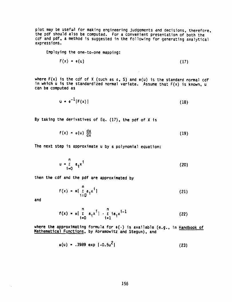
plot maybe useful for making engineering judgements and decisions, therefore,the pdf should also be computed. For a convenient presentation of both thecdf and pdf, a method is suggested in the following for generating analyticalexpressions.

Employing the one-to-one mapping:

F(x) : _(u) (17)

where F(x) is the cdf of X (such as 6, S) and ®(u) is the standard normal cdf

in which u is the standardized normal variate. Assume that F(x) is known, ucan be computed as

u = _-IIF(x)] (18)

By taking the derivatives of Eq. (17), the pdf of X is

duf(x)= ®(u) (19)

The next step is approximate u by a polynomial equation:

n i

u = z aix (20)i=O

then the cdf and the pdf are approximated by

n

F(x) = '[i--_I)alxl) (21)

and

n n

f(x)- oIi.oZ alxlI • _:l!alxl-li (22)

where the approximating formula for ¢(.) is available (e.g., in Handbook ofMathematical Functions, by Abramowitz and Stegun), and

¢(u) - .3g89 exp [-0.Su2) (23)

156

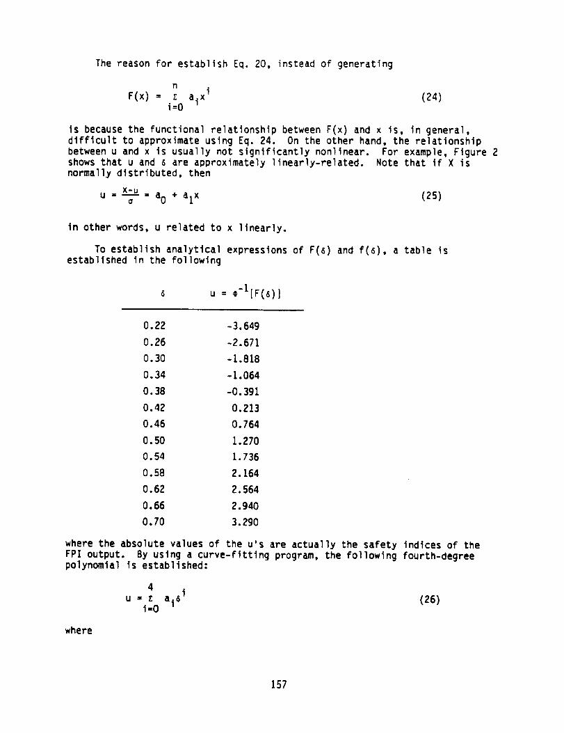
The reason For establish Eq. 20, instead of generating

n

F(x) : _ aixl (24)i=O

is because the functional relationship between F(x) and x is, in general,

difficult to approximate using Eq. 24. On the other hand, the relationship

between u and x is usually not significantly nonlinear. For example, Figure 2shows that u and 6 are approximately linearly-related. Note that if X is

normally distributed, then

u = x----V-ua" ao + alx (25)

in other words, u related to x linearly.

To establish analytical expressions of F(6) and f(6), a table isestablished in the following

u : _-l[F(6)]

0.22 -3.649

0.26 -2.671

0.30 -1.818

0.34 -I.064

O. 38 -0.391

0.42 0.213

0.46 0.764

0.50 1.270

0.54 1.736

0.58 2. 164

O. 62 2.564

0.66 2.940

0.70 3.290

where the absolute values of the u's are actually the safety indices of the

FPl output. By using a curve-fitting program, the following fourth-degreepolynomial is established:

4

u - _: ai6i (26)i--O

where

157

a0 = -12.1307

aI = -54.6602

a2 = -90.7163

a3 = 87.4329

a4 = -34.9088

For the values of 6 computed, the relative errors in u estimates are

approximately less than one percent.

By substituting the coefficients of Eq. 26 into Eq. 22, it is now

convenient to compute f(6). Figure 3 shows the plot of f(6) using Eq. 22.

The above procedure of presenting the result of the reliability analysisfor the tip displacement can be applied for the maximum stress.

A Monte Carlo simulation with sample size of 100,000 resulted in

S = 7294 psi

By substituting the medians of the random variables into Eq. 14, the stress is

S = 7330 psi

which is near the simulation result.

Thirteen values of the cdf of S are computed and listed in Table 3. The

result is also plotted on a normal probability paper (Figure 4). There is

almost no difference between the simulation (sample size = 100,000) and theFPl results.

The analytical expressions of F(s) and f(s) are given by Eq. 17 and Eq.19 where

4

u = z aiSi (27)i=O

in which

a0 = -12.1726

aI = 2.88859

a2 = -0.245685

a3 = 0.0127482

a4 = -0.000278666

a f(s) plot using these coefficients is shown in Figure 5.

158

The probability that the stress exceeds the yield strength requires onlyone run of the FPI program. The result is

pf = 0.0511 (FPI)= 0.0510 (Monte Carlo with sample size = 100,004))

The pdf of the yield strength is also plotted in Figure S to compare with the

pdf of the stress. The pdf of strength, which is Weibully-distributed, is

where

= 12.0226

a : 10.4342 ksi

159

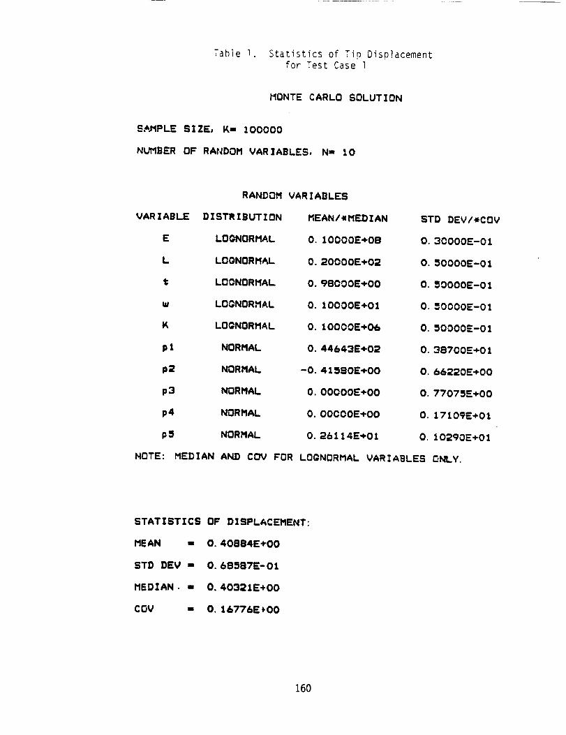
Table 1 Stacistics of Tip Displacement

for Test Case 1

MONTE CARLO SOLUTION

S_PLE SIZE, K- I00000

NUMBER OF RANDOM VARIABLES, N- I0

RANDOM VARIABLES

VARIABLE DISTRIBUTION MEAN/_MEDIAN STD DEV/*COV

E LOONORMAL 0.10000E+OB 0.30000E-01

L LOgNORMaL 0.20000E+02 0.50000E-01

t LOONORMAL 0.98000E÷00 0.50000E-01

w LO_NORMAL 0.10000E+01 0.50000E-01

K LOONORMAL 0.10000E+O_ 0.50000E-01

pl NORMAL 0.44643E+02 0.38700E+01

p2 NORMAL -0.41590E_00 0.66220E÷00

p3 NORMAL O. O0000E+O0 O. 77075E+00

p4 NORMAL O. OOO00E÷O0 0.17109E+01

p5 NORMAL 0.26114E÷01_ 0.10290E+01

NOTE: MEDIAN AND COV FOR LOgNORMAL VARIABLES _NLY.

STATISTICS OF DISPLACEMENT:

MEAN m 0.40884E÷00

STD DEV = 0.6BSB7E-01

MEDIAN. m 0.40321E+00

COY - 0.1a77aE,O0

160

Table 2. The cdf of the Tip Displacement (Case I)

Displacementinch

0.22

0.26

0.30

0.34

0.38

0.42

0.46

0.50

0.54

0.58

0.62

0.66

0.70

cdf

aMonte Carlo FPI

0.000169 0.000132

0.00468 0.00378

0.0385 ' 0.0346

0.152 0.144

0.362 0.348

O.596 0.585

0.785 0.777

0.901 0.898

0.9606 0.9586

0.9858 0.9848

0.9953 0.9948

0.99842 0.99836

0.99966 0.999498

a: Sample size = 100,000

161

Table 3. The cdf of the Maximum Stress (Case I)

Stress

ksi

4.4

cdf

aMonte Carlo FPI

0.000590 0.000599

5.06

5.72

6.38

7.04

7.70

8.36

g.02

g.68

i0.34

11.00

11.66

12.32

0.00890 0.00876

0.0545 0.0548

0.188 0.185

0.404 0.400

0.636 0.634

0.816 0.814

0.922 0.920

0.972 0.9703

0.99107 0.99023

0.99724 0.99712

0.99912 0.999219

0.99966 0.999803

a: Sample size = 100,000

162

Modeled Using a Torsion Spring

Pl

P4t

Z

P5

Z

FIGURE I. Model Definition of a Cantilever Beam

163

0

uc

co

I=

m}

J(_)

Figure 2.

• Monte Carlo

(Sample size =

The cdf of the tip displacement (Case l)

Ill

• FPI

III

lOO,OOO)

III

!!!

'i'

Iii

Li

illIII

If|

I ' "

IIIIIIi I •

IIIII!

..... ii| w

I'

11I , "I

L

I I i ,

I

if

.3 .4

Di sl)lacemeni'.,inch

164

4_

E

(J

f,..=

e-,(/.i

o_,..

,,.m

-r-

l,-

o

l,

t...

.i,.,=

d

d

0

d

0

d

0

U¢,,.

EU

0_

I-'-

uo!_,_un..-I ,_:l.!sueG ,_.!l!qt_clo_d

165

:}°_

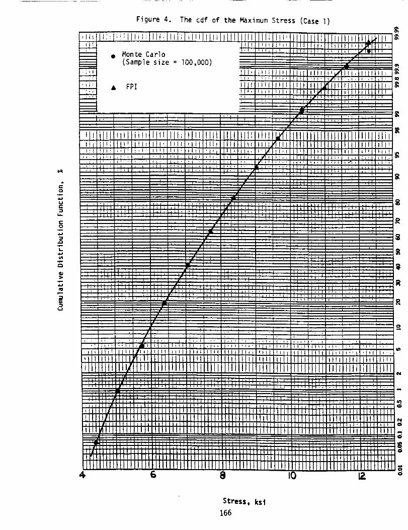
U

C

o

,,Q

Figure 4.

ll:;l;_)illi:i

• Monte Carlo(Sample size :

• FPI

The cdf of the Maximum Stress

1oo,ooo)Ii

ii

. r

II

(Case l)

i

! ....

8 o

Stress, ksl

166

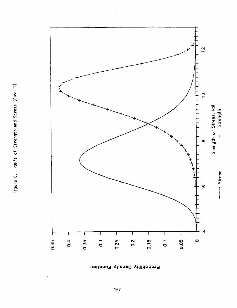
l/1G.If,,.

S..

0

I.I.

L

It1

0

uo!_oun 3 /_,!muoc] ,_.!l!qOclOJd

167

l.i_

II

II

i

Illtli!illtl_tlli!lltiiiltltititlttllll!

• MONTE CARLO

( N-, IOO,OOO )

!!!tltl!l!lll I_IIIi I

illltllII [

• FPI

I

i_ i,_i!ii!Itlili! Ili,l"

I

J

I

!I

I

i• I

, I

li

IIiq

i

i

t

II

I

!I

8

I

li ,

I

i

Ill I

ItllI,li

ii_II1

Ill

Ill

I0

IIIIIII

illiil!

I1':, !,ll,i ,

III

II1

i[

I

tl,,

.11

llli

_ iI!! "

I

STRESS ,168

KSI

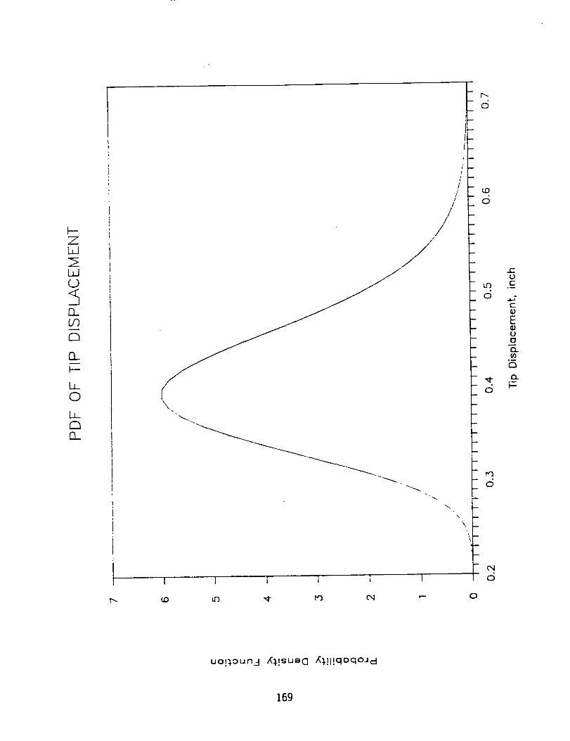
F-ZLLI

LLJL.)

ELU')

r'_

0._

t--

LLC)

LL

£L

/!/

/

//

/

\

\.

I I 1 I I I

r--,

-c;

! -

CO

-(5

U'3

-(5

_t"

-(5

I.-

(5

eQ

(5

.E(...)t-

.,l..a

E

Ee.)(J0

EL

r'_

t_o_

I---

uo!_.:3un-I ,K_.!gug(] _.]l]qDqoJ d

169

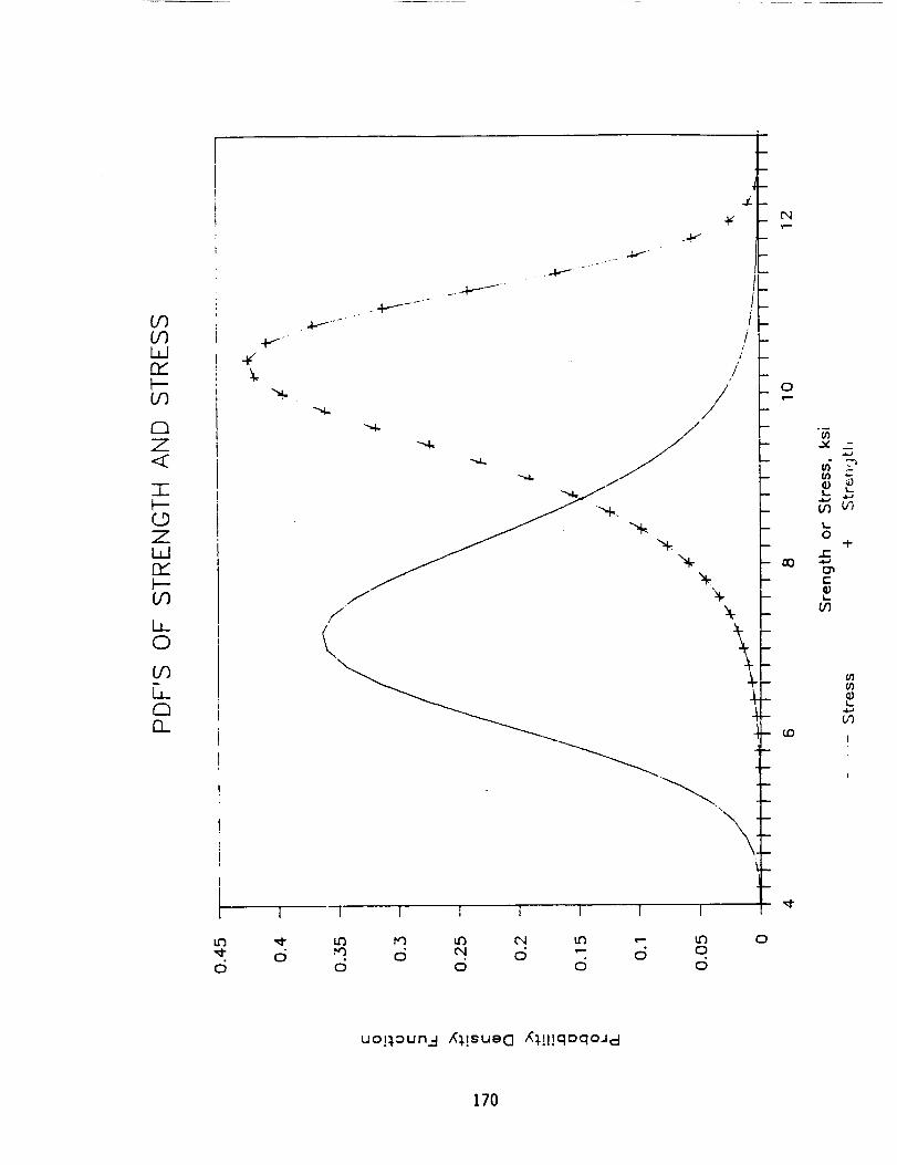
wn_

r-_Z<

-F

ZWnIp-

b_©

O_

-_ _l.f " //I _

_'

i ®

, ._ _

i I [ I I I I I I

C_ 0 0 0 0

0

uo!_,oun...-I ,_,!sueQ ,,{_.!l!qoqoa=l

170

Section 5

Non-normal Correlated Vectors in Structural Reliability Analysis

Dr. Y.-T. Wu

Southwest Research Institute

October 1985

171

Introduction

In structural reliability analysis, techniques are well developed for

computing the probability measures of a given performance function, g(X) ,

where X=(X1,X2, ... Xn) an independent vector. For example, fast probability

integration (FPI) methods are currently being used in the PSAM project.

However, it is not uncommon that the basic stochastic variables, Xi's , such asthe geometrical parameters, the loadings, etc., are dependent and non-normal.

If the Joint probability distribution function of the X can be defined,

the Rosenblatt transformation {I], as suggested by Hohenbichler and Rackwitz,may be employed to generate an independent, normal vector [2). Then the FPI

methods may be used. Unfortunately, in practical applications, the underlyingjoint distribution functions are very difficult to construct based on either

theory or experiment. Moreover, the Rosenblatt transformation involves the

inversion of the conditional distribution functions which are, in general,extremely difficult to derive or to compute numerically. This is particularly

true for the cases involving large numbers of design random variables whichare typical in the PSAM project.

Another way of solving the dependency problem is to use the marginal

distributions and the correlation coefficients, which are relatively easy toobtain. It is well known that an orthogonal transformation can be employed touncouple the dependency. If, in addition, the correlated variables areassumed normally distributed, then the transformed vector will be normal and

independent. On the other hand, however, if the correlated variables cannot

be assumed normally distributed, the distributions of the transformedindependent vector are unknown and the FPI methods cannot be used.

The problem associated with non-normal correlated vector has been

addressed in the literature [3,41. For example, Der Kiureghian and Liusuggested that the bivarlate distribution model due to Natal (51 can beused. The transformed normal correlation coefficients between each two

variables were found by Iteratively solving a double integral equation.Because the calculation is tedious, a set of seml-emplrical formulae for

selected marginal distributions were developed.

In this study, a different approach employing series expansion isdeveloped for solving the transformed normal correlation coefficients. The

method is general and efficient, suitable for complicated distributions.

Examples are provided to demonstrate the capabilities of the approximationmethod. Finally, the possible applications to the PSAM project are discussed.

Problem Definition

Given a non-normal vector X with marginal distributions, i.e., the

cumulative distribution functions (cdf's) Fxi(Xl) (i=l, n), the covariancematrix _X may be constructed as

172

where

CX --

D

C11 C12 ... Cln

Cnl ... Cnn

(1)

cij = E[XlXjl - E[XiIE[XjI(2)

in which E[.] are the expected values. The correlation coefficients, PX 'are defined as iXj

(3)

where oI and oj are the standard deviations (std.) of Xi and Xj, respectively.

Using the bivariate normal distribution model, the normal distributions

are established first by the following transformations:

FxI(x i) : <>i(ui)i=l,n (4)

where ¢(.) is the normal cdf and ui is a standard normal variate. Note that

Eq. 4 defines a one-to-one mapping; therefore, xI may be formulated using theinverse transformation:

Xi = Fx "l(¢i(ui) ) (S)t

The inverse cdf's, i.e., FXt-I(. ) are available in closed forms for

distributions such as Weibull and extreme value. For many distributionmodels, the closed form solutions do not exist; and for a given uvalue, x must be solved iteratively.

The next step is to find the correlation coefficients oij between any ui

and uj (i#J). To simplify the presentation of the analysis, consider I=i and

J=2, and let _ = 012 (the "normal" correlation coefficient), o can be found

by solving the following double integration equation.

oxI//lX2(xl-ul)(x2-u2)_12dUldU 2 (6)

173

where ui = the meanvalues,

I u_- 2pUlU2 + u_exp [- ] (7)

_12 = 2_ 1_o2 2(1-o 2)

and Xl, X2 are to be transformed to u1, u2 using Eq. 5. In general, there is

no closed form solution for Eq. 6, and the calculation of o requires

iteratively solving Eq. 6. The process is particularly cumbersome when the

inverse transformation (i.e., Eq. 5) also needs to be solved iteratively.

Nevertheless, if all the o's are obtained for the corresponding OXiXj,

which means that the covarlance matrix of u vector is established, then an

orthogonal transformation may be employed to construct an independent normal

vector suitable for rellabillty analysis. In the following dlscussion, an

alternative procedure for computing o's will be developed which avoids the useof the double integral.

Obtaining the Normal Correlation Coefficients

Using Series Expansion - A New Approach

Consider two correlated random variables, denoted as XI and X2.

correlation coefficients PXIX2 can be computed as

The

EIXIX 2] - E[XIIE[X21Z

°XIX 2 01o 2(8)

Define the transformation from Xi to ui as

Xi = Ti(ui) i=I, 2 (g)

and define

H(u I, u2) = XIX 2 = T1(ul)T2(uz) (I0)

Eq. 8 may be expressed as

OXtX2OlO2 = EIH] - E[T1]E[T2](Ii)

174

Expand H into Taylor series about the point (uI, u2) = (0,0),

H = HO0 + _(H20u I + 2H11UlU 2 + Ho2U ) + H.O.T. (12)

where H.O.T. = Higher Order Terms

diTi dJT 2

uo u=O

(13)

Eq. 11 can be written as

PXIX2 +I°2 = HO0 + 1 H2oE[U_] + 2HllE[UlU2] + Ho2E(u_) ÷ E[H.O.TI

(14)

- E[T1] - E[T2]

luJ can be derived using the moment generatingThe expected values of uI 2

function. For example, it can be shown that:

E[UlU 2) = o

E[u_) --I

E[u_] = 0

22E[UlU21 = I + 2o2

etc.

(IS)

iJA derivation of E[UlU 2] up to i+j=8 has been carried out and is listed in

Table I. By using Eq. 15, Eq. 14 simplifies to

PXIX2alo2 = HO0 + ½ (H20 + 2PHI1 + H02)

+ E[H.O.T.I-E[T 1] - E[T2]

(16)

175

Applying the condition that 0=0 whenPXIX2=O,Eq. 16 further reduces to

_XIX2ala2 = OHll + EIH.O.T.I (17)

Therefore, a rough approximation, neglecting the fourth and hlgher-order(third-order coefficient is zero) terms, is simply

ala 2

= H-_ °XlX2 (18)

in which

dT I dT2

u=O(19)

where Ti defines the transformations, e.g., Eq. 5.

If Ti are linear, e.g., when Xi are normal distributions, with

means ui and standard deviations ai, then

XI = Ti(u) = uI + uI oI (20)

Employing Eq. 19 gives

Hli = Ola 2 (21)

and Eq. 8 then degenerates to

" (22)1Xz

as expected.

In general, TI are non-llnear functions of u4, therefore, Eq. 18 is a good

approximation only'when Xi are not significantly _on-normal. Using Table I, amore complete approximation formula, up to eighth-order terms of H series wasderived as:

176

_XiX2Ola2= o[H11+ 21-(H13+H31)+ l(HIs+2H33+Hs1) + 1(H17+3H35*3Hs3+H71)]

2 "

+ _'-[H22 + l(H24+H42) + l(H26+2H14+H62)]

3 (23)+ _--[H33 + 1(H53+H35)]

4

+ "_4[ H441

This equation is believed to be adequate for the practical problems involving

highly non-llnear transformations. The inclusions of even higher-order terms

are straight forward using Eq. 23.

The procedure of computing o may be outlined in the following steps,

suitable for computer programming:

I.

o

Select N (say N=9) points of u values, e.g., from -4 to +4, with

increments of I. Compute Xi=T(ui) (i=1, 2) for the N values of u.

For both T1 and T_, find the (N-l)th order approximating polynomials

using prop(r numeFical schemes.

3. Compute Hij using the result of step 2.

4. Solve o From Eq. 23.

For small coefficient of variations (COV's), say COV < 0.15, typical of

the engineering problems, the fourth-order approximation provides a relatively

efficient way of computing o. The equation is

2

OXiX2ala2 = =[H11+_(H31+H13)] * _- H22(24)

The highest derivatives for XI and X2 are the third orders and o may be foundby solving a quadratic equati6n.

Examples

To demonstrate how to use the derived formula, and to examine the

accuracy, consider the following examples.

Example [ - XI and X2 are both 1ognormally distributed, with equal COV's =

C. The transformations are:

177

CnXi-"Yi) = $(u i)(x) = ®(FX i i

°Yi

(25)

or

Xi = exp[uy + uio Y 1i I

(26)

where Yi = _nXi(i=t'2) and

- ui

uyl= LnX I = _nJ I,cz

g!

(27)

=v/ tn(l+C2) '= Oy°Y I

(2B)

where Xi is the median of Xi.

From Eq. 26

dRX_= n

du; o yiexpiry i* uiOy ]

(29)

It follows that

HIj = (Oy)i+Jexp[_yl+Uyz](30)

Substltutlng Eq. 30 into Eq. 23 without truncating the series, and using Eq.

27, it can be shown that

DXIX2C 2 = exp[=o_]-I(31)

178

Therefore,

_n(1+OXIX2 C2)(32)

= _n(1+C 2)

which is an exact solution. The more general solution for the case CI#C 2

derived using a similar approach is

Ln(I+oxIX2ClC2 )D = (33)

v/ _n(1+C_)In(1+C_)'

In general, closed-form solutions may be very difficult to derive or

simply doesn't exist. In this case, a proper truncating series may be used.In the following, the effect of nonlinear transformation and the effect of

truncating the series will be discussed using the two lognormal variablescase.

Recall that the nonlinear transformation of a lognormal variable X to a

normal u is

X = Xexp[u_n / 1+C 2 ' ] (34)

Ignoring the constant X, the functional relationship between X and u isplotted in Figure I for three values of C, namely C=0.I, C=0.3 and C=0.5.shows clearly that the C values significantly affect the nonlinearity of

X=T(u) around u=O.

Now consider the truncated series. Assume that CI = 0.1 and C2 = 0.5,the exact solution is:

It

= 21.222 zn[1+.O5oxIX2]

and the approximating solution, using Eq. 23, is

(35)

179

•05618OXIX2 = o[.04712+.005492+.00032+.000012431

+ o2[.00111+.0001294+.00000754]

(36)+ _3[.00001744+. 000002031

+ o4[.000000205J

where It Is evident that the series converges quickly.

let PXIX2 = 0.9 , the results are as follows:

o (Second-order approx.) = 1.192

(Fourth-order approx.) = 0.9423

D (Sixth-order approx.) = 0.9345

(Eighth-order approx.) = 0.9341

o (Exact) = 0.9341

It may be observed that (for PXIX2 > 0 case)

As an example,

ala 2

H11 P)(tX2 > Pexact > PXIX 2 (37)

which means that the second-order approximation (using Hli and oi only)

provides an upper bound of exact p. Note that Ipl(Exact)_IPXiX21 has been

proven (e.g., see Lancaster [61). An important application of Eq. 37 is thatIf the bounds are judged narrow enough, then it is not necessary to try to

obtain very accurate o value.

Example 2. Consider the case where one (say Xl) of the two variables isnormally distributed, then

dXl =

oI (3s)

180

dnX 1-Oforn>l (39)

at Ul=O.

The approximating series of Eq. 23 simplifies to

°XlX2 °2 = o.L1 [Hll + ½ H13+ 1 H15+ 1 H17]

d3x 2dx2 1 _ +

=otd- Z+ du l u2=o

(40)

where o is not a function of XI.

Assume that X? is a lognormal variable with median of unity and COV of0,5. Pretend that-the differentiation of x, with respect to u, Is difficult

and therefore must be done numerically. Using the strategy suggested earlier,nine sets of solutions are obtained as follows:

Set u2 T(u2)

1 -4 0.1511

2 -3 0.2424

3 -2 O. 3887

4 -1 0.6235

5 0 1.0

6 1 1.6038

7 2 2. 5722

8 3 4.1253

9 4 6.6162

The function T(u2) was plotted in Figure I.

The next step is to construct an eighth-order polynomlal denoted as

181

8

c AnU_x2 = n=O

The required derivatives for computing p are

(41)

dnx 2

u2=O

=A.n'n

(42)

where n-l, 3, 5 and 1.

By solving nine simultaneous linear equations, the coefficients are foundaS:

A1 = 0.472353

A3 = 0.017595

A5 - 0.000191

A7 = O.00OO13

Using Eq. 42 and Eq. 40, the approximation solution is

= 1.0584 PXlX2

The exact solution can be derived as:

C2s s

°J n(l*C )°XlX2 l"OS84°XlX2

(43)

(44)

which proves that the proposed algorithm works very wet1.

Applications

Before discussing the possible applications, it is worthwhile to note

that: (a) the correlations between the design variables may have significant

effect on structural analysis (e.g., see Thoft-Christensen [6]), and (b) In

probablllstic finite element analysis, the loading as well as the geometrymust be discretized. For small element size, correlations usually exist

between adjacent elements.

182

Let us consider a long bar. The cross-sectional area may be treated as a

random variable. By discretizing the bar into n elements, there are n areas,

A_, each of which is a random variable. If the element lengths are relativelysBort, then It would be unrealistic to assume that the adjacent Ai are

independent because the independency suggests the sudden changes in areas. On

the other hand, Ai's cannot be assumed perfectly correlated if, in reality,

Ai's are changing along the bar.

A possible solution to this problem is to treat the area (along the bar)

as a random process. If the bars are manufactured under quality control, thenit seems reasonable to further assume that the random process is stationary.

Under the above assumptions, the marginal distribution as well as the

correlations may be extracted from the measurement data. Obviously, the area

need not be normally distributed.

The above discussion may be extended to two dimensional problems. For

example, the thickness of a nominally flat plate may be treated as astationary random process. The correlation functions may be constructed alongdifferent directions. This approach is, in fact, very similar as in defining

a correlation field of random loading.

The treatment of the material property, e.g., modulus of elasticity

(again, may be non-normal) as a correlated; but not perfectly correlated,random field is much more involved because it would be difficult to obtain

experimental data for small elements. Correlation function needs to be

assumed or established using other material properties which are related to

the strength of material (e.g., Brlnell Hardness Number). For the PSAM

project, the selections of the correlations need to be tailored to thespecific problem under investigation. For example, the modulus of elasticity

of a turbine blade may be considered perfectly correlated. However, some

independency may be assumed among different blades.

Assuming that the correlation functions are defined for the elements, thecorrelated non-normal variables can be transformed to independent normal

variables using the procedure proposed earlier. Because the number of

variables may be large, it is suggested that the orthogonal transformationshould be done on a zone-by-zone basis where a zone is defined as a region in

which the variables are correlated; there is negligible correlation outside

this region. Since the number of variables in each zone is relatively small,

the computation time may be reduced significantly.

Summary,

Given a non-normal dependent vector with marginal distributions and

correlation coefficients, a method using series expansion was developed for

obtaining approximating correlation coefficients of the transformed jointnormal distributions. Then the orthogonal transformation may be implemented

to obtain independent normal vectors suitable for FPI or other reliability

analysis.

Several levels of approximations were obtained and their accuracies and

usefulness discussed. For example, the second-order approximation (using only

Hli ), which is easy to obtain, may provide a close bound of the exact

183

solutlon. The series expansion has been derived up to eighth-order, which

should be adequate for the problems encountered in the PSAM project. A simplenumerical algorithm was suggested for computer programming.

Flnally, in discussing the appllcations of the developed method, it was

suggested that the geometries, the material properties, etc., may be treated

as non-normal dependent vectors, and that the orthogonal transformation shouldbe performed on a zone-by-zone basis.

References

Io Rosenblatt, M., "Remarks on a Multivariate Transformation," Annals of

Mathematical Statistics, Vol. 23, No. 3, Sept. 1952, pp. 470-472.

o Hohenbichler, M., and Rackwitz, R., "Non-Normal Dependent Vectors in

Structural Safety," Journal of the Engineering Mechanics Division, ASCE,Vol. 100, No. EM6, Dec. 1981, pp. 1227-1238.

s

8

Der Klureghian, A., and Llu, P.-L., "Structural Rellability Under

Incomplete Probability Information," Report No. UCB/SESM-85/OI,

Department of Civil Engineering, University of California, Berkeley.

Grlgoriu, M., "Approximate Analysis of Complex Rellability Problems,"Structural Safety, 1, 1983, pp. 277-288.

e Johnson, N.L., and Kotz, S., "Distributions in Statistics - Continuous

Multivariate Distributions," John Wiley & Sons, Inc., New York, N.Y.,1976.

o Lancaster, H.O., "Some Properties of Blvarlate Normal Distribution

Considered in the Form of a Contingency Table," Blometrika, Vol. 44, pp.289-292, June 1957.

o Thoft-Christensen, P., and Baker, M. J., "Structural Reliability Theoryand Application," Springer-Verlag, 1982.

184

Table i

Expected Values of the Functions of Two Correlated

Standard Normal Variables (u, v)

FUNCTION ORDER EXPECTED VALUE

U, V

u 2

UV

2

2

2

0

1

0

u3,v3,u3v,uv2 0

u4,v 4

u3v,uv 3

u2v 2

3

3o

1+2_ 2

u5,v5,u4v,uv 4, etc.

u6,v 6

u5v, uv 5

u4v2,u2v 4

u3v 3

15

15o

3+12o 2

9p+6o 3

uT,vl,u6v,uv 6, etc.

u8,v 8

ulv,uv /

u6v2,u2v6

uSv3,u3v 5

u4v 4

8

8

8

8

8

105

105o

15+90o 2

450+6003

9+7202+2404

185

X : T(u)

8C=0.5

4

J_ l+C2 'X = exp[u n( )]

C=0.3

I I I-2 0 2 4

C=O]

U

Figure 1. Nonlinear Transformation of a Lognormal Variable

186

I Form ApprovedREPORT DOCUMENTATION PAGE OMB NO. 0704-0188

Public reporting burden for this collection of information is estimated to average 1 hour per response, including the time for reviewing instructions, searching existing data sources,

gathering and maintaining the data needed, and completing and reviewing the collection of information. Send comments regarding this burden estimate or any other aspect of this

collection of iolormallon, inCluding suggestions for reducing this burden, to Washington Headquarters Services, Directorate for information Operations and Reports, 1215 Jefferson

Davis H_ghway, Suite 1204, Arlington, VA 22202-4302, and to the Office ol Management and Budget, Paperwork Reduct)on Project (0704-0188), Washington, DC 20503.

April 1992 Final Contractor Report

5. FUNDING NUMBERS4. TITLE AND SUBTITLE

Probabilistic Structural Analysis Methods for Select Space Propulsion

System Components (PSAM)

Volume Ill-Literature Surveys and Technical Reports

6. AtrrHoR(S)

7. PERFORMING ORGANIZATION NAME(S) AND ADDRESS(ES)

Southwest Research Institute6220 Culebra Road

San Antonio, Texas 78228

9. SPONSORING/MONITORING AGENCY NAMES(S) AND ADDRESS(ES)

National Aeronautics and Space AdministrationLewis Research Center

Cleveland, Ohio 44135-3191

WU-590--21-11

C-NAS3--24389

8. PERFORMING ORGANIZATIONREPORT NUMBER

None

10. SPONSORING/MONITORINGAGENCY REPORT NUMBER

NASA CR-189159

11. SUPPLEMENTARY NOTES

Project Manager, e.G. Chamis, Structures Division, NASA Lewis Research Center, (216) 433-3252.

121. DISTRIBUTION/AVAILABILITY STATEMENT

Unclassified - Unlimited

Subject Category 3912b.

DISTRIBUTION CODE

13. ABSTRACT (Maximum 200 words)

This annual report summarizes the technical effort and computer code developed during the first year. Several

formulations for Probabilistic Finite Element Analysis (PFEA) are described with emphasis on the selected formula-

tion. The strategies being implemented in the first-version computer code to perform linear, elastic PFEA is

described. The results of a series of select Space Shuttle Main Engine (SSME) component surveys are presented.

These results identify the critical components and provide the information necessary for probabilistic structural

analysis. The report is issued in three volumes: Volume I - summarizes theory and strategies; Volume II - summa-

rizes surveys of critical space shuttle main engine components; and Volume III - summarizes literature surveys and

technical reports available at that time.

14. SUBJECT TERMS

Finite elements; Strategy; Computer code; Space shuttle main engine; Select compo-

nents; Literature; Survey

17. SECURITYoFREPORTunclassifiedCLASSIFICATION118. I

NSN 7540-01-280-5500

SECURITY CLASSIFICATIONOF THIS PAGE

Unclassified

19. SECURITY CLASSlRCATIONOF ABSTRACT

Unclassified

15. NUMBER OF PAGES188

16. PRICE CODEA00

20. LIMITATION OF ABSTRAC

Standard Form 298 (Rev. 2-89)Prescribed by ANSI SKI. Z39-18298-102