l1 monge-kantorovich problem with applications · 2017-05-02 · l 1 monge-kantorovich problem with...
TRANSCRIPT
L1 Monge-Kantorovich problem with applications
Stanley Osher
UCLA
May 2, 2017
Joint work with Wilfrid Gangbo, Wuchen Li, Yupeng Li, Ernest Ryu, BaoWang, Penghang Yin and Wotao Yin.
Partially supported by ONR and DOE.
Outline
Introduction
Method
Models and ApplicationsUnbalanced optimal transportImage segmentationImage alignment
Introduction 2
Motivation
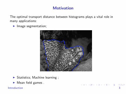
The optimal transport distance between histograms plays a vital role inmany applications:
I Image segmentation;
I Statistics; Machine learning ;
I Mean field games .
Introduction 3
Motivation
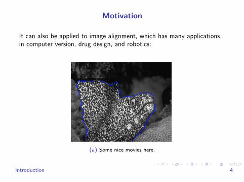
It can also be applied to image alignment, which has many applicationsin computer version, drug design, and robotics:
(a) Some nice movies here.
Introduction 4
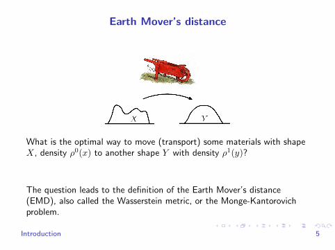
Earth Mover’s distance
What is the optimal way to move (transport) some materials with shapeX, density ρ0(x) to another shape Y with density ρ1(y)?
The question leads to the definition of the Earth Mover’s distance(EMD), also called the Wasserstein metric, or the Monge-Kantorovichproblem.
Introduction 5
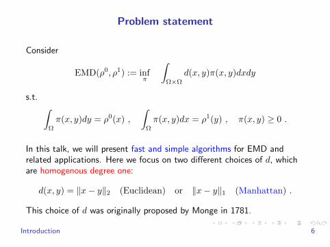
Problem statement
Consider
EMD(ρ0, ρ1) := infπ
∫Ω×Ω
d(x, y)π(x, y)dxdy
s.t. ∫Ω
π(x, y)dy = ρ0(x) ,
∫Ω
π(x, y)dx = ρ1(y) , π(x, y) ≥ 0 .
In this talk, we will present fast and simple algorithms for EMD andrelated applications. Here we focus on two different choices of d, whichare homogenous degree one:
d(x, y) = ‖x− y‖2 (Euclidean) or ‖x− y‖1 (Manhattan) .
This choice of d was originally proposed by Monge in 1781.
Introduction 6
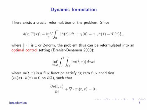
Dynamic formulation
There exists a crucial reformulation of the problem. Since
d(x, T (x)) = infγ∫ 1
0
‖γ(t)‖dt : γ(0) = x , γ(1) = T (x) ,
where ‖ · ‖ is 1 or 2-norm, the problem thus can be reformulated into anoptimal control setting (Brenier-Benamou 2000):
infm,ρ
∫ 1
0
∫Ω
‖m(t, x)‖dxdt
where m(t, x) is a flux function satisfying zero flux condition(m(x) · n(x) = 0 on ∂Ω), such that
∂ρ(t, x)
∂t+∇ ·m(t, x) = 0 .
Introduction 7
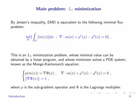
Main problem: L1 minimization
By Jensen’s inequality, EMD is equivalent to the following minimal fluxproblem:
infm∫
Ω
‖m(x)‖dx : ∇ ·m(x) + ρ1(x)− ρ0(x) = 0 .
This is an L1 minimization problem, whose minimal value can beobtained by a linear program, and whose minimizer solves a PDE system,known as the Monge-Kantorovich equation:
p(m(x)) = ∇Φ(x) , ∇ ·m(x) + ρ1(x)− ρ0(x) = 0 ,
‖∇Φ(x)‖ = 1 ,
where p is the sub-gradient operator and Φ is the Lagrange multiplier.
Introduction 8
Outline
Introduction
Method
Models and ApplicationsUnbalanced optimal transportImage segmentationImage alignment
Method 9
L1 minimization
From numerical purposes, the minimal flux formulation has two benefits
I The dimension is much lower, essentially the square root of thedimension in the original linear optimization problem.
I It is an L1-type minimization problem, which shares structure withproblem arising in compressed sensing. We borrow a very fast andsimple algorithm used there.
Method 10
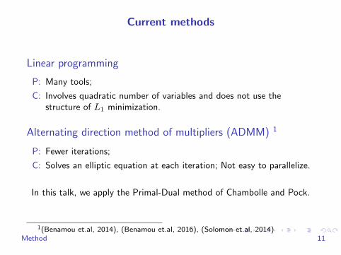
Current methods
Linear programming
P: Many tools;
C: Involves quadratic number of variables and does not use thestructure of L1 minimization.
Alternating direction method of multipliers (ADMM) 1
P: Fewer iterations;
C: Solves an elliptic equation at each iteration; Not easy to parallelize.
In this talk, we apply the Primal-Dual method of Chambolle and Pock.
1(Benamou et.al, 2014), (Benamou et.al, 2016), (Solomon et.al, 2014)Method 11

Settings
Introduce a uniform grid G = (V,E) with spacing ∆x to discretize thespatial domain, where V is the vertex set and E is the edge set.i = (i1, · · · , id) ∈ V represents a point in Rd.
Consider a discrete probability set supported on all vertices:
P(G) = (pi)Ni=1 ∈ RN |N∑i=1
pi = 1 , pi ≥ 0 , i ∈ V ,
and a discrete flux function defined on the edge of G :
mi+ 12
= (mi+ 12 ev
)dv=1 ,
where mi+ 12 ev
represents a value on the edge (i, i+ ev) ∈ E,
ev = (0, · · · ,∆x, · · · , 0)T , ∆x is at the v-th column.
Method 12
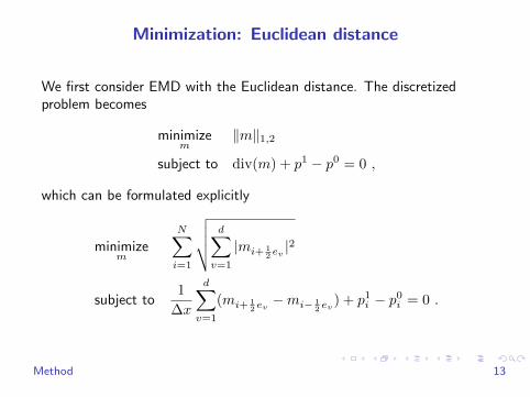
Minimization: Euclidean distance
We first consider EMD with the Euclidean distance. The discretizedproblem becomes
minimizem
‖m‖1,2
subject to div(m) + p1 − p0 = 0 ,
which can be formulated explicitly
minimizem
N∑i=1
√√√√ d∑v=1
|mi+ 12 ev|2
subject to1
∆x
d∑v=1
(mi+ 12 ev−mi− 1
2 ev) + p1
i − p0i = 0 .
Method 13
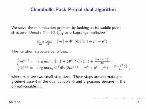
Chambolle-Pock Primal-dual algorithm
We solve the minimization problem by looking at its saddle pointstructure. Denote Φ = (Φi)
Ni=1 as a Lagrange multiplier:
minm
maxΦ
‖m‖+ ΦT (div(m) + p1 − p0) .
The iteration steps are as follows:mk+1 = arg minm ‖m‖+ (Φk)Tdiv(m) +
‖m−mk‖222µ ;
Φk+1 = arg maxΦ ΦTdiv(2mk+1 −mk + p1 − p0)− ‖Φ−Φk‖222τ ,
where µ, τ are two small step sizes. These steps are alternating agradient ascent in the dual variable Φ and a gradient descent in theprimal variable m.
Method 14
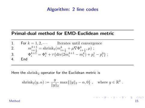
Algorithm: 2 line codes
Primal-dual method for EMD-Euclidean metric
1. For k = 1, 2, · · · Iterates until convergence
2. mk+1i+ 1
2
= shrink2(mki+ 1
2
+ µ∇Φki+ 1
2
, µ) ;
3. Φk+1i = Φki + τdiv(2mk+1
i −mki ) + p1
i − p0i ;
4. End
Here the shrink2 operator for the Euclidean metric is
shrink2(y, α) :=y
‖y‖2max‖y‖2 − α, 0 , where y ∈ R2 .
Method 15
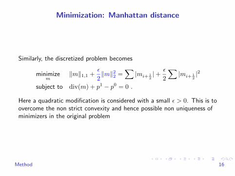
Minimization: Manhattan distance
Similarly, the discretized problem becomes
minimizem
‖m‖1,1 +ε
2‖m‖22 =
∑|mi+ 1
2|+ ε
2
∑|mi+ 1
2|2
subject to div(m) + p1 − p0 = 0 .
Here a quadratic modification is considered with a small ε > 0. This is toovercome the non strict convexity and hence possible non uniqueness ofminimizers in the original problem
Method 16
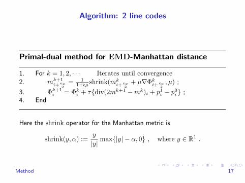
Algorithm: 2 line codes
Primal-dual method for EMD-Manhattan distance
1. For k = 1, 2, · · · Iterates until convergence
2. mk+1i+ ev
2= 1
1+εµ shrink(mki+ ev
2+ µ∇Φki+ ev
2, µ) ;
3. Φk+1i = Φki + τdiv(2mk+1 −mk)i + p1
i − p0i ;
4. End
Here the shrink operator for the Manhattan metric is
shrink(y, α) :=y
|y|max|y| − α, 0 , where y ∈ R1 .
Method 17
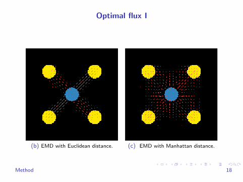
Optimal flux I
(b) EMD with Euclidean distance. (c) EMD with Manhattan distance.
Method 18

Optimal flux II
(d) EMD with Euclidean distance. (e) EMD with Manhattan distance.
Method 19

Manhattan vs Euclidean
Grids number (N) Time (s) Manhattan Time (s) in Euclidean100 0.0162 0.1362400 0.07529 1.6451600 0.90 12.2656400 22.38 130.37
Table: We compute an example for Earth Mover’s distance with respect toManhattan or Euclidean distance.
This is result by using Matlab in a serial computer. In a parallel codeusing CUDA, it takes around 1 second to find a solution in a 256× 256grid for the Euclidean metric. It speeds up roughly 104 times.
Method 20
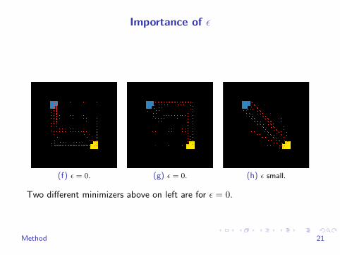
Importance of ε
(f) ε = 0. (g) ε = 0. (h) ε small.
Two different minimizers above on left are for ε = 0.
Method 21
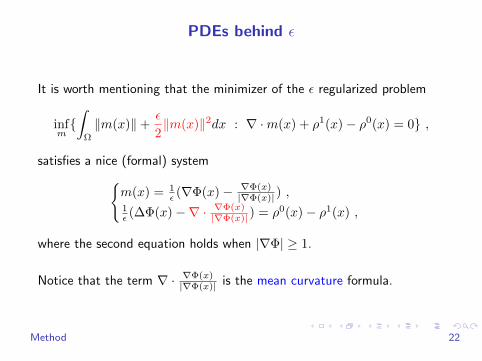
PDEs behind ε
It is worth mentioning that the minimizer of the ε regularized problem
infm∫
Ω
‖m(x)‖+ε
2‖m(x)‖2dx : ∇ ·m(x) + ρ1(x)− ρ0(x) = 0 ,
satisfies a nice (formal) systemm(x) = 1
ε (∇Φ(x)− ∇Φ(x)|∇Φ(x)| ) ,
1ε (∆Φ(x)−∇ · ∇Φ(x)
|∇Φ(x)| ) = ρ0(x)− ρ1(x) ,
where the second equation holds when |∇Φ| ≥ 1.
Notice that the term ∇ · ∇Φ(x)|∇Φ(x)| is the mean curvature formula.
Method 22
Outline
Introduction
Method
Models and ApplicationsUnbalanced optimal transportImage segmentationImage alignment
Models and Applications 23
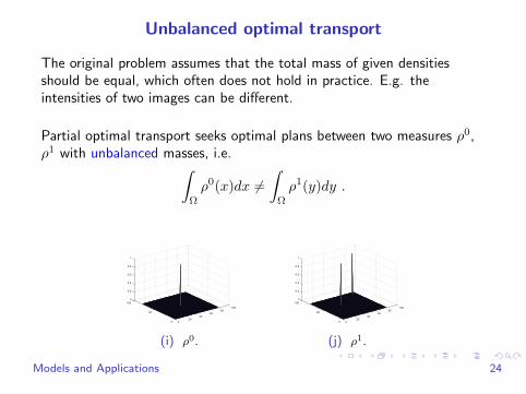
Unbalanced optimal transport
The original problem assumes that the total mass of given densitiesshould be equal, which often does not hold in practice. E.g. theintensities of two images can be different.
Partial optimal transport seeks optimal plans between two measures ρ0,ρ1 with unbalanced masses, i.e.∫
Ω
ρ0(x)dx 6=∫
Ω
ρ1(y)dy .
100
80
60
40
20
00
50
1
0.8
0.6
0.4
0.2
0
100
(i) ρ0.
100
80
60
40
20
00
50
1
0
0.2
0.4
0.6
0.8
100
(j) ρ1.
Models and Applications 24
Unbalanced optimal transport
A particular example is the weighted average of Earth Mover’s metric andL1 metric, known as Kantorovich-Rubinstein norm. One importantformulation is
infu,m∫
Ω
‖m(x)‖dx : ∇ ·m(x) + ρ0(x)− u(x) = 0 , 0 ≤ u(x) ≤ ρ1(x) .
Our method can solve the problem by 3 line codes.
Models and Applications 25
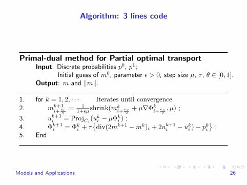
Algorithm: 3 lines code
Primal-dual method for Partial optimal transportInput: Discrete probabilities p0, p1;
Initial guess of m0, parameter ε > 0, step size µ, τ , θ ∈ [0, 1].Output: m and ‖m‖.
1. for k = 1, 2, · · · Iterates until convergence
2. mk+1i+ ev
2= 1
1+εµ shrink(mki+ ev
2+ µ∇Φki+ ev
2, µ) ;
3. uk+1i = ProjCi
(uki − µΦki ) ;
4. Φk+1i = Φki + τ
div(2mk+1 −mk)i + 2uk+1
i − uki )− p0i
;
5. End
Models and Applications 26
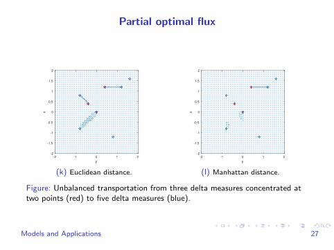
Partial optimal flux
y
-2 -1 0 1 2
x
-2
-1.5
-1
-0.5
0
0.5
1
1.5
2
(k) Euclidean distance.
y
-2 -1 0 1 2
x
-2
-1.5
-1
-0.5
0
0.5
1
1.5
2
(l) Manhattan distance.
Figure: Unbalanced transportation from three delta measures concentrated attwo points (red) to five delta measures (blue).
Models and Applications 27
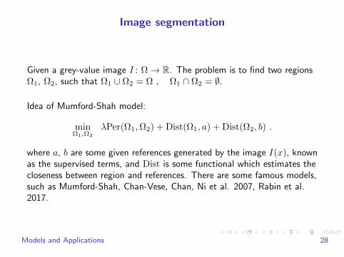
Image segmentation
Given a grey-value image I : Ω→ R. The problem is to find two regionsΩ1, Ω2, such that Ω1 ∪ Ω2 = Ω , Ω1 ∩ Ω2 = ∅.
Idea of Mumford-Shah model:
minΩ1,Ω2
λPer(Ω1,Ω2) + Dist(Ω1, a) + Dist(Ω2, b) .
where a, b are some given references generated by the image I(x), knownas the supervised terms, and Dist is some functional which estimates thecloseness between region and references. There are some famous models,such as Mumford-Shah, Chan-Vese, Chan, Ni et al. 2007, Rabin et al.2017.
Models and Applications 28
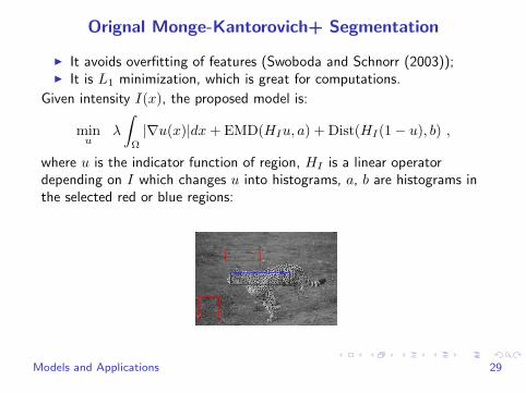
Orignal Monge-Kantorovich+ Segmentation
I It avoids overfitting of features (Swoboda and Schnorr (2003));I It is L1 minimization, which is great for computations.
Given intensity I(x), the proposed model is:
minu
λ
∫Ω
|∇u(x)|dx+ EMD(HIu, a) + Dist(HI(1− u), b) ,
where u is the indicator function of region, HI is a linear operatordepending on I which changes u into histograms, a, b are histograms inthe selected red or blue regions:
Models and Applications 29
Problem formulation
infu,m1,m2
λ
∫Ω
‖∇xu(x)‖dx+
∫F‖m1(y)‖dy +
∫F‖m2(y)‖dy ,
where the infimum is taken among u(x) and flux functions m1(y), m2(y)satisfying
0 ≤ u(x) ≤ 1
∇y ·m1(y) +HI(u)(y)− a(y)
∫FHI(u)(y)dy = 0
∇y ·m2(y) +HI(1− u)(y)− b(y)
∫FHI(1− u)(y)dy = 0 .
Here x ∈ Ω, y ∈ F , HI : BV(Ω)→ Measure(F) is a linear operator.
Our algorithm can be easily used into this area. It contains only 6 simpleand explicit iterations using the Chamolle-Pock primal dual method.
Models and Applications 30
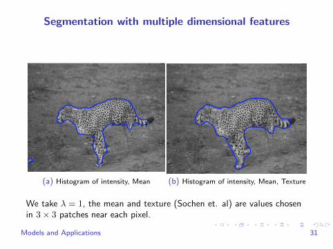
Segmentation with multiple dimensional features
(a) Histogram of intensity, Mean (b) Histogram of intensity, Mean, Texture
We take λ = 1, the mean and texture (Sochen et. al) are values chosenin 3× 3 patches near each pixel.
Models and Applications 31
Segmentation with multiple dimensional features
(c) Histogram of intensity, Mean (d) Histogram of intensity, Mean, Texture
Models and Applications 32
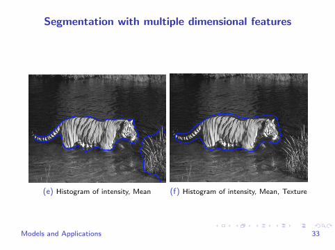
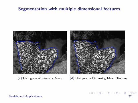
Segmentation with multiple dimensional features
(e) Histogram of intensity, Mean (f) Histogram of intensity, Mean, Texture
Models and Applications 33
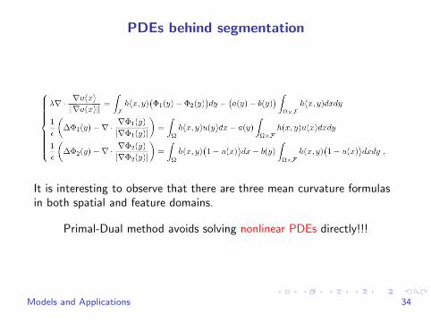
PDEs behind segmentation
It is interesting to observe that there are three mean curvature formulasin both spatial and feature domains.
Primal-Dual method avoids solving nonlinear PDEs directly!!!
Models and Applications 34
Image alignment via Monge-Kantorovich problem
Models and Applications 35
Discussion
Our method for solving L1 Monge-Kantorovich related problems
I handles the sparsity of histograms;
I has simple updates and is easy to parallelize;
I introduces a novel PDE system (Mean curvature formula in MongeKantorovich equation).
It has been successfully used in partial optimal transport, imagesegmentation, image alignment and elsewhere.
Models and Applications 36
Main references
Wuchen Li, Ernest Ryu, Stanley Osher, Wotao Yin and WilfridGangbo.A parallel method for Earth Mover’s distance, 2016.
Wuchen Li, Penghang Yin and Stanley Osher.A Fast algorithm for unbalanced L1 Monge-Kantorovich problem,2016.
Yupeng Li, Wuchen Li and Stanley Osher.Image segmentation via original Monge-Kantorovich problem, inprepration.
Penghang Yin, Bao Wang, Wuchen Li and Stanley Osher.A Fast algorithm for unbalanced L1 Monge-Kantorovich problem, inpreparation.
Models and Applications 37

Thanks!
Models and Applications 38