l12: template matching - cs course webpagescourses.cs.tamu.edu/rgutier/csce689_s11/l12.pdfl12:...

Introduction to Speech Processing | Ricardo Gutierrez-Osuna | CSE@TAMU 1

L12: Template matching

• Introduction to ASR

• Pattern matching

• Dynamic time warping

• Refinements to DTW

This lecture is based on [Holmes, 2001, ch. 8]


Introduction to ASR

• What is automatic speech recognition? – The goal of ASR is to accurately and efficiently convert a speech signal

into a text message transcription of the spoken words

– This process should be independent of

• The device used to record the speech (i.e., the microphone)

• The speaker’s characteristics (i.e., age, gender, accent)

• The acoustic environment (i.e., quiet office vs. noisy rooms, outdoors)

– The ultimate goal, which has yet to be achieved, is to perform as well as a human listener would


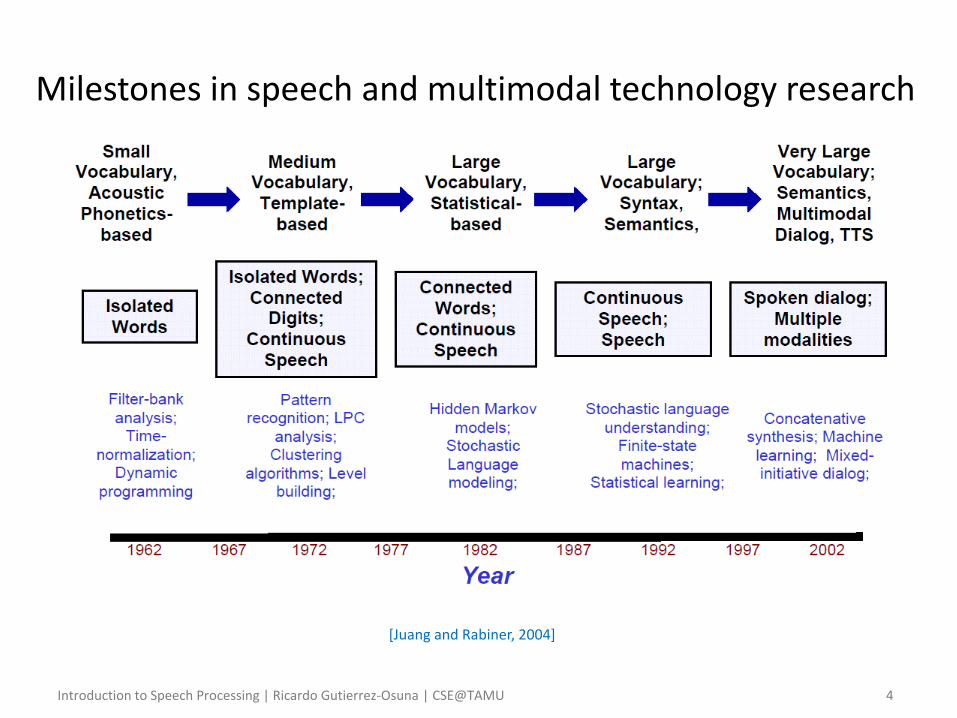
• History of ASR – Rule-based methods

• Early work starting in the 1950s focused on developing of rules based on (1) acoustic-phonetic knowledge (i.e. formants), or (2) ad-hoc measurements of properties of the speech signal

• These systems could recognize digit and isolated words, but performed poorly because of (1) coarticulation effects and (2) the inflexibility of rule-based hard decisions

– Template-matching • During the 1960s and 1970s, work on ASR benefited from developments

in pattern matching techniques, particularly dynamic time warping

• These systems worked reasonably well at isolated word recognition, but did not properly use information about variability in the speech signal

– Statistical modeling • During the 1970s and 1980s, research on ASR moved towards statistical

methods for acoustic and language modeling

• These methods (e.g., hidden Markov models, n-grams) have now been almost universally adopted for ASR


[Juang and Rabiner, 2004]

Milestones in speech and multimodal technology research


[Rabiner and Schafer, 2007]

Overall architecture of a modern ASR system


• Lecture plan – In this lecture, we will review early work on pattern matching and the

use of dynamic time warping (DTW)

• Though DTW has been largely superseded, the algorithm still finds uses in other areas of speech research

– The second lecture on ASR will focus on hidden Markov models (HMM), their basic structure and learning algorithms

– The third lecture will cover refinements for HMMs, including issues of robustness and speaker independence

– The fourth lecture will discuss large-vocabulary ASR, including acoustic and language modeling, and decoding

– The fifth lecture will introduce HTK, the most widely used software for research and development in ASR


Pattern matching

• Basis for the approach – As we have previously seen, the relationship between acoustic

patterns and their linguistic content is quite complex, partly due to coarticulation

– However, if the same person repeats the same isolated word on separate occasions, the pattern is likely to be similar, particularly when looking at spectrograms

– This suggests one potential approach for ASR

• Store examples of acoustic patterns (call them templates) for all the words to be recognized

• For an incoming word, compare it with each of the stored patterns and assign it to the closest match


• Distance metrics – Assume for now that the words are spoken in isolation, at exactly the

same speed, and that the start/end points can be easily detected

• We will soon see how to relax this unrealistic assumptions

– In this case, the distance between words may be computed as

• Divide words into short-time frames (e.g., 10-20 ms)

• Compute a feature vector for each frame (e.g., DFT)

• Calculate Euclidean distance for each pair of frames

• Sum up distances across frames


• What makes good feature vectors for ASR? – With the exception of tonal languages (e.g., Mandarin), pitch

information generally does not carry much phonetic information

• Thus, the feature vector should ignore harmonic structure and instead focus on the spectral envelope of the signal

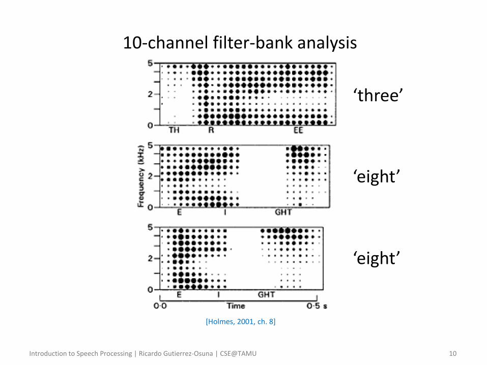
– A reasonable approach is to perform a filter-bank analysis following an auditory frequency scale (e.g., Mel, critical bands), and then compute the log-power at each channel

• The log-power ensures that weaker formants (which may be of linguistic significance) are properly weighted in the distance measure

• We may also subtract the average log-power of each word to cancel differences in vocal effort or distance to the microphone


10-channel filter-bank analysis

‘three’

‘eight’

‘eight’

[Holmes, 2001, ch. 8]


Euclidean distance between words

Similar Different

[Holmes, 2001, ch. 8]


• End-point detection – Our earlier approach assumes that the start and end points for each

word are known or can be easily found

– One may detect end-points by means of a simple level threshold

• This approach, however, may fail when words start or end with weak sounds (e.g., [f])

• Words may also have periods of silence within them (e.g., ‘containing’)

• Other problems include speaker artifacts (lip clicking, exhalation, etc.)

– Improvements in end-point detection can be achieved by accounting for the spectral properties of the background noise

• However, despite its apparent simplicity, end-point detection is often unreliable


• Allowing for timescale variation – Up to now we have also assumed that words to be compared are of

the same length and that the corresponding frames represent the same phonetic features

– In practice, speakers use different speaking rates, and these rates are non-uniform (see earlier slide with two STFT for the word ‘eight’)

– Fortunately, these issues can be addressed by “aligning” the two words with a mathematical technique known as dynamic time warping


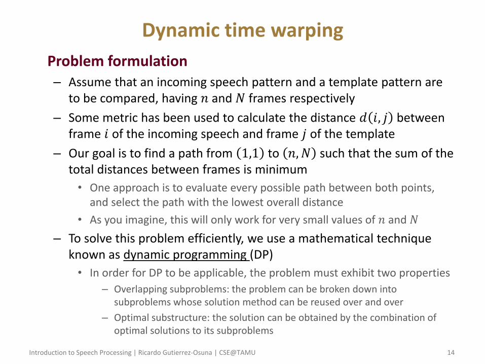
Dynamic time warping

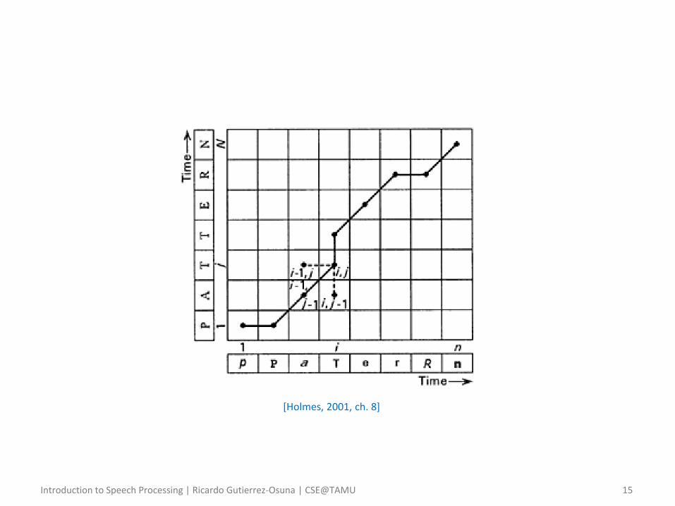
• Problem formulation – Assume that an incoming speech pattern and a template pattern are

to be compared, having 𝑛 and 𝑁 frames respectively

– Some metric has been used to calculate the distance 𝑑 𝑖, 𝑗 between frame 𝑖 of the incoming speech and frame 𝑗 of the template

– Our goal is to find a path from 1,1 to 𝑛, 𝑁 such that the sum of the total distances between frames is minimum

• One approach is to evaluate every possible path between both points, and select the path with the lowest overall distance

• As you imagine, this will only work for very small values of 𝑛 and 𝑁

– To solve this problem efficiently, we use a mathematical technique known as dynamic programming (DP)

• In order for DP to be applicable, the problem must exhibit two properties

– Overlapping subproblems: the problem can be broken down into subproblems whose solution method can be reused over and over

– Optimal substructure: the solution can be obtained by the combination of optimal solutions to its subproblems


[Holmes, 2001, ch. 8]


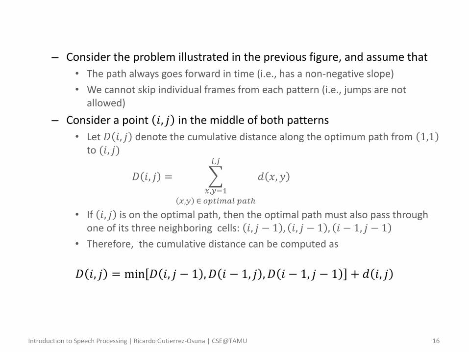
– Consider the problem illustrated in the previous figure, and assume that

• The path always goes forward in time (i.e., has a non-negative slope)

• We cannot skip individual frames from each pattern (i.e., jumps are not allowed)

– Consider a point 𝑖, 𝑗 in the middle of both patterns

• Let 𝐷 𝑖, 𝑗 denote the cumulative distance along the optimum path from 1,1 to (𝑖, 𝑗)

𝐷 𝑖, 𝑗 = 𝑑 𝑥, 𝑦

𝑖,𝑗

𝑥,𝑦=1

𝑥,𝑦 ∈ 𝑜𝑝𝑡𝑖𝑚𝑎𝑙 𝑝𝑎𝑡ℎ

• If 𝑖, 𝑗 is on the optimal path, then the optimal path must also pass through one of its three neighboring cells: 𝑖, 𝑗 − 1 , 𝑖, 𝑗 − 1 , 𝑖 − 1, 𝑗 − 1

• Therefore, the cumulative distance can be computed as

𝐷 𝑖, 𝑗 = min 𝐷 𝑖, 𝑗 − 1 , 𝐷 𝑖 − 1, 𝑗 , 𝐷 𝑖 − 1, 𝑗 − 1 + 𝑑 𝑖, 𝑗


– In other words, the best way to get to 𝑖, 𝑗 is to get to one of its immediately preceding points by the best way, and then take the appropriate step to 𝑖, 𝑗

– Thus, a simple procedure may be used to fill in matrix 𝐷

• Initialization: 𝐷 1,1 = 𝑑 1,1

• Cells along the left-hand side can only follow one direction (vertical), so starting with 𝐷 1,1 , values for 𝐷 1, 𝑗 can be calculated for increasing values of 𝑗

• Once the left column is completed, the second column can be computed

from 𝐷𝑖,𝑗 = min 𝐷𝑖,𝑗−1, 𝐷𝑖−1,𝑗 , 𝐷𝑖−1,𝑗−1 + 𝑑𝑖,𝑗, and so forth

– The value obtained for 𝐷 𝑛,𝑁 is the score for the best way of matching the two words

– If you also are interested in finding the optimal path itself, then additional book-keeping is necessary to backtrack from 𝐷 𝑛,𝑚 to 𝐷 1,1


ex12p1.m Aligning utterances with DTW


Refinements to DTW

• Penalties for time-scale distortions – DTW works best when both words have similar lengths, otherwise the

path will contain a large number of vertical and horizontal segments

– Although the presence of these segments will implicitly penalize the overall cost of the path, it is sometimes advisable to penalize them explicitly

𝐷 𝑖, 𝑗 = min

𝐷 𝑖 − 1, 𝑗 + 𝑑 𝑖, 𝑗 + 𝒉𝒅𝒑

𝐷 𝑖 − 1, 𝑗 − 1 + 2𝑑 𝑖, 𝑗

𝐷 𝑖, 𝑗 − 1 + 𝑑 𝑖, 𝑗 + 𝒗𝒅𝒑

– where the value of horizontal and vertical distortion penalties (vdp,hdp) must be determined empirically

• Length normalization – The cumulative distance depends on the length of the example and

the template, so the best-match decision will favor short templates

– To remove this bias, one can divide the total distance by the length of the template


• Score pruning – DP provides very significant savings when compared to evaluating

every possible path, but remains computationally intensive when there is a large number of templates to be matched

– Additional savings can be obtained by not allowing path with relatively bad scores to propagate forward

• As an example, it is unlikely that a cell whose cumulative distance 𝐷 𝑖, 𝑗 far exceeds the minimum in its column will be part of the minimal path

– Thus, one could prune any paths continuing from that cell

• In doing so, we trade-off optimality with potentially significant savings (i.e., speedup by a factor of 5-10)

– Note, however, that most circumstances where pruning is likely to eliminate the optimal path will be those when the two words are different, in which case overestimating the cumulative distance will not affect recognition rates


DTW alignment between two examples of the word ‘eight’ with score pruning but no time-scale distortion

[Holmes, 2001, ch. 8]

DTW alignment between two examples of the word ‘eight’ with score-pruning AND a small time-scale distortion; notice the more plausible matching of the two timescales

DTW alignment between two dissimilar words (‘three’ and ‘eight’) with time-scale distortion; score pruning was removed as the resulting path would have been seriously suboptimal

l12: template matching - cs course webpagescourses.cs.tamu.edu/rgutier/csce689_s11/l12.pdfl12:...

Documents