l2:vuq.p2.03 brian adams snl completed: 3/31/11 · software tools, characterizing uncertainties,...

L2:VUQ.P2.03 Brian Adams

SNL Completed: 3/31/11

CASL-U-2011-0049-000

SANDIA REPORT SAND2011-2238 Unlimited Release Printed April 2011

CASL L2 Milestone Report: VUQ.Y1.03, “Enable Statistical Sensitivity and UQ Demonstrations for VERA” Brian M. Adams Walter R. Witkowski Yixing Sung Prepared by Sandia National Laboratories Albuquerque, New Mexico 87185 and Livermore, California 94550

Sandia National Laboratories is a multi-program laboratory managed and operated by Sandia Corporation, a wholly owned subsidiary of Lockheed Martin Corporation, for the U.S. Department of Energy's National Nuclear Security Administration under contract DE-AC04-94AL85000. Approved for public release; further dissemination unlimited.

CASL-U-2011-0049-000

2

Issued by Sandia National Laboratories, operated for the United States Department of Energy by Sandia Corporation. NOTICE: This report was prepared as an account of work sponsored by an agency of the United States Government. Neither the United States Government, nor any agency thereof, nor any of their employees, nor any of their contractors, subcontractors, or their employees, make any warranty, express or implied, or assume any legal liability or responsibility for the accuracy, completeness, or usefulness of any information, apparatus, product, or process disclosed, or represent that its use would not infringe privately owned rights. Reference herein to any specific commercial product, process, or service by trade name, trademark, manufacturer, or otherwise, does not necessarily constitute or imply its endorsement, recommendation, or favoring by the United States Government, any agency thereof, or any of their contractors or subcontractors. The views and opinions expressed herein do not necessarily state or reflect those of the United States Government, any agency thereof, or any of their contractors. Printed in the United States of America. This report has been reproduced directly from the best available copy. Available to DOE and DOE contractors from U.S. Department of Energy Office of Scientific and Technical Information P.O. Box 62 Oak Ridge, TN 37831 Telephone: (865) 576-8401 Facsimile: (865) 576-5728 E-Mail: [email protected] Online ordering: http://www.osti.gov/bridge Available to the public from U.S. Department of Commerce National Technical Information Service 5285 Port Royal Rd. Springfield, VA 22161 Telephone: (800) 553-6847 Facsimile: (703) 605-6900 E-Mail: [email protected] Online order: http://www.ntis.gov/help/ordermethods.asp?loc=7-4-0#online

CASL-U-2011-0049-000

3

SAND2011-2238 Unlimited Release Printed April 2011

CASL L2 Milestone Report: VUQ.Y1.03, “Enable Statistical Sensitivity and UQ

Demonstrations for VERA”

Brian M. Adams Optimization and Uncertainty Quantification

Walter R. Witkowski

Validation and Uncertainty Quantification Processes

Sandia National Laboratories P.O. Box 5800

Albuquerque, New Mexico 87185-1318

Yixing Sung Westinghouse Nuclear Fuel

Westinghouse Electric Company LLC

1000 Westinghouse Drive Cranberry Township, Pennsylvania, 16066

Abstract

The CASL Level 2 Milestone VUQ.Y1.03, “Enable statistical sensitivity and UQ demonstrations for VERA,” was successfully completed in March 2011. The VUQ focus area led this effort, in close partnership with AMA, and with support from VRI. DAKOTA was coupled to VIPRE-W thermal-hydraulics simulations representing reactors of interest to address crud-related challenge problems in order to understand the sensitivity and uncertainty in simulation outputs with respect to uncertain operating and model form parameters. This report summarizes work coupling the software tools, characterizing uncertainties, selecting sensitivity and uncertainty quantification algorithms, and analyzing the results of iterative studies. These demonstration studies focused on sensitivity and uncertainty of mass evaporation rate calculated by VIPRE-W, a key predictor for crud-induced power shift (CIPS).

CASL-U-2011-0049-000

4

ACKNOWLEDGMENTS This work was funded by and conducted under the auspices of the DOE CASL Energy Innovation Hub for Modeling & Simulation for Nuclear Reactors, led by Oak Ridge National Laboratory, in which Sandia National Laboratories is a core partner. The work is part of a cross-focus area CASL effort involving its VUQ, VRI, and AMA program elements. It benefitted from coordinating support by CASL focus area leads Jim Stewart (SNL), John Turner (ORNL), and Zeses Karoutas (Westinghouse). This sensitivity and uncertainty demonstration study relied on problem statements, models, and technical guidance provided by Westinghouse Electric Company LLC. Other direct contributors included Chris Baker (ORNL), Rose Montgomery (TVA), Jeff Secker (Westinghouse), Laura Swiler (SNL), and Brian Williams (LANL). Computational hardware and support was provided by SNL’s Computer Science Research Institute.

CASL-U-2011-0049-000

5

CONTENTS

1. Overview .................................................................................................................................... 9

2. Computational Models and Algorithms ................................................................................... 11 2.1. VIPRE-W simulations .................................................................................................. 11 2.2 DAKOTA Overview ..................................................................................................... 13 2.3. DAKOTA Algorithms Applied ..................................................................................... 14

3. Uncertainty Characterizations and DAKOTA Specifications ................................................. 19 3.1 PWR Plant A Parameters and Uncertainties ................................................................. 19 3.2 PWR Plant B Parameters and Uncertainties ................................................................. 20

4. Sensitivity and Uncertainty Results ......................................................................................... 23 4.1. Results for Plant A ........................................................................................................ 24

4.1.1. Comparison of Sensitivity Analysis Techniques ............................................ 24 4.1.2. Comparison of Uncertainty Quantification Techniques ................................. 27

4.2. Results for Plant B ........................................................................................................ 29 4.2.1. Comparison of Sensitivity Analysis Techniques ............................................ 29 4.2.2. Comparison of Uncertainty Quantification Techniques ................................. 32

5. Discussion ................................................................................................................................ 39

6. References ................................................................................................................................ 41

Appendix A: Sample Analysis Files ............................................................................................ 43

Distribution ................................................................................................................................... 46

FIGURES Figure 1. VIPRE-W output demonstrating execution on Odin cluster at SNL with appropriate group ownership. ........................................................................................................................... 12 Figure 2. VIPRE-W quarter core geometry and channel layout. .................................................. 13 Figure 3. Loose (“black-box”) coupling of DAKOTA to a generic application. ......................... 14 Figure 4. Matrix of scatter plots for parameters versus responses; based on the 400 sample LHS study of the Plant A model. ........................................................................................................... 25 Figure 5. PSUADE/MOAT modified mean versus standard deviation in elementary effects for ME_mean response. ...................................................................................................................... 27 Figure 6. Plant A response distribution fits to analytical statistical distributions. ........................ 28 Figure 7. Goodness of fit test of normality on ME_mean. ........................................................... 29 Figure 8. Scatter plots of inputs versus responses for Plant B, LHS 1000 samples. .................... 30 Figure 9. Plant B: MOAT statistics for ME_max response based on 990 model evaluations. ..... 32 Figure 10. Best-fit distributions for Plant B outputs, based on 1000 LHS samples. .................... 34 Figure 11. Test for normality of response ME_max for Plant B, based on 1000 samples. .......... 35 Figure 12. Plot of mean of mass evaporation rate (taken over 100 LHS samples) at each node in the Plant B computational model. ................................................................................................. 36 Figure 13. Plot of mean of mass evaporation rate viewed from above the Plant B core. ............. 36

CASL-U-2011-0049-000

6

Figure 14. Plot of standard deviation of mass evaporation rate (taken over 100 LHS samples) at each node in the Plant B computational model. ............................................................................ 37 Figure 15. Plot of standard deviation of mass evaporation rate viewed from above the Plant B core. ............................................................................................................................................... 37 Figure 16. Representative DAKOTA input file for performing Latin hypercube sampling for Plant A. ......................................................................................................................................... 43 Figure 17. Shell script runvipre_massevap.sh iteratively called by DAKOTA. ........................... 44 Figure 18. Shell script massevap_stats.sh used to post-process VIPRE-W output to generate metrics of interest for return to DAKOTA. .................................................................................. 45

TABLES Table 1. DAKOTA variable names associated with VIPRE-W operating and model parameters........................................................................................................................................................ 19 Table 2. Plant A, typical core operating parameter uncertainties. ................................................ 20 Table 3. Plant A, corresponding DAKOTA normal distributions. ............................................... 20 Table 4. Plant B, typical parameters for SA, UQ, calibration, and validation studies. ................. 20 Table 5. Plant B, corresponding DAKOTA normal distributions. ............................................... 21 Table 6. Plant B, corresponding DAKOTA uniform distributions. .............................................. 21 Table 7. Summary of SA and UQ metrics reported for each method type. .................................. 23 Table 8. DAKOTA response names corresponding to derived VIPRE-W system responses. ..... 24 Table 9. Simple correlations between inputs and outputs for Plant A, 4000 sample LHS analysis........................................................................................................................................................ 25 Table 10. Partial Correlation Matrix for Plant A, 4000 Sample LHS Analysis. ........................... 25 Table 11. PCE-based Sobol’ Indices for Plant A ME_mean response. ........................................ 26 Table 12. 3rd order PCE-based Sobol’ indices for all Plant A responses. ..................................... 26 Table 13. PSUADE/MOAT results for 4000 sample study (statistics on elementary effects). .... 27 Table 14. Comparison of response means and standard deviations calculated by DAKOTA LHS and PCE methods for the Plant A model. ..................................................................................... 28 Table 15. Correlations for Plant B 1000 sample LHS analysis. ................................................... 30 Table 16. PCE Sobol’ indices for ME_mean response for varying quadrature order. ................. 31 Table 17. Sobol’ indices for all responses, 3rd order quadrature PCE case. ................................ 31 Table 18. Plant B summary of elementary effects based on 990 MOAT evaluations. ................. 32 Table 19. Comparison of Response Means and Standard Deviations Using Different UQ Techniques for Plant B Model ...................................................................................................... 33

CASL-U-2011-0049-000

7

NOMENCLATURE AMA Advanced Modeling Applications (CASL technical focus area) AOA Axial offset anomaly CASL Consortium for Advanced Simulation of LWRs CIPS Crud-induced power shift DAKOTA Design and Analysis ToolKit for Optimization and Terascale Applications DOE Department of Energy EPRI Electric Power Research Institute LANL Los Alamos National Laboratory LWR Light water reactor m-dot-e Mass evaporation rate ORNL Oak Ridge National Laboratory PWR Pressurized water reactor SA Sensitivity analysis SNL Sandia National Laboratories UQ Uncertainty quantification TVA Tennessee Valley Authority VBD Variance-based decomposition VERA Virtual Environment for Reactor Applications VIPRE-W Thermal hydraulics subchannel simulator code (Fortran) VRI Virtual Reactor Integration (CASL technical focus area) VUQ Validation and Uncertainty Quantification (CASL technical focus area) Westinghouse Westinghouse Electric Company LLC

CASL-U-2011-0049-000

8

CASL-U-2011-0049-000

9

1. OVERVIEW Analysis and improved scientific understanding of crud formation on nuclear fuel rod surfaces and its impact on operating light water reactors (LWRs), such as Crud-induced power shift (CIPS), are central to the mission of the Consortium for Advanced Simulation of LWRs (CASL) DOE Energy Innovation Hub. The CASL Level 2 Milestone VUQ.Y1.03, “Enable statistical sensitivity and UQ demonstrations for VERA,” executed jointly with the AMA and VRI focus areas, directly supports better understanding of these reactor performance-critical phenomena by performing DAKOTA studies on VIPRE-W thermal-hydraulics simulations of reactors of interest. This milestone primarily consists of a capability demonstration study focused on thermal hydraulics simulations of two Westinghouse-designed four-loop pressurized water reactors (PWRs) conducted with the VIPRE-W software. The first simulation, “PWR Plant A,” was the reference plant for the CASL project as defined by the AMA team. The second scenario, “PWR Plant B,” is targeted for a validation data study based on crud-related measurements from a plant similar to the reference plant, in which CIPS occurred in a previous operating cycle. While studies conducted with Plant A are exploratory, the Plant B scenario was selected as it will be the object of study in consequent calibration and validation exercises, demonstrating a complete VUQ workflow. DAKOTA algorithms assessed the influence of thermal hydraulic parameters on mass evaporation rate (a predictor for crud formation) throughout two quarter core models of Plants A and B. Sensitivity analysis (SA) determined the influence of thermal-hydraulic parameters on mass evaporation rate to rank their relative importance, while uncertainty quantification (UQ) assessed the mean and variance of the mass evaporation rate, with respect to input parameter uncertainties. Completion of this milestone required:

compiling VIPRE-W and requisite third-party libraries on SNL platforms; developing job submission, execution, and post-processing scripts to couple DAKOTA to

VIPRE-W; characterizing the uncertainty in input parameters and creating corresponding DAKOTA

input files for various SA and UQ methods; performing sensitivity and uncertainty studies with various levels of refinement; and analyzing and summarizing the results.

In turn, this report summarizes the VIPRE-W simulations of interest, the DAKOTA algorithms applied for SA and UQ, the parameters studied and their characterizations of uncertainty, and prototypical results from the various algorithms used.

CASL-U-2011-0049-000

10

CASL-U-2011-0049-000

11

2. COMPUTATIONAL MODELS AND ALGORITHMS This section offers an introduction to the VIPRE-W simulations for Plants A and B, the DAKOTA tool overall, and the specific algorithms applied for SA and UQ. Both software tools were executed on the Odin commodity cluster, housed in the Computer Science Research Institute at SNL. 2.1. VIPRE-W Simulations VIPRE-W is a Westinghouse version of the VIPRE-01 code. VIPRE-01 is a thermal-hydraulic subchannel code based on the COBRA codes developed by Pacific Northwest National Laboratories under sponsorship of the Electric Power Research Institute (EPRI) [1]. VIPRE-W contains enhancements for PWR applications, including the mass evaporation and grid spacer heat transfer models required for CIPS risk assessment. VIPRE-W and its third-party libraries were compiled and installed on Odin, a computer cluster hosted on SNL’s restricted (non-public) network. The VIPRE-W installation as well as all analysis files and generated outputs associated with the study were protected with a UNIX group caslvuq, together with appropriate permissions, as demonstrated by the simulation output header shown in Figure 1.

CASL-U-2011-0049-000

12

Figure 1. VIPRE-W output demonstrating execution on Odin cluster at SNL with

appropriate group ownership. Simulations for the two four-loop PWR cores were both based on the quarter core geometry shown in Figure 2, with 193 flow channels (shown) and 93 nodes with a nodal length of about 50 mm (2 inches) in the axial direction (not shown). Each flow channel represents a quarter of a fuel assembly. Baseline VIPRE-W input decks were furnished by Westinghouse.

Copyright (c) Westinghouse Electric Company, 2010 All Rights Reserved Westinghouse Nuclear Fuel Westinghouse Proprietary ‐ Class 2 Computer Code VIPRE‐W, Version 7.12.A File: /projects/home/briadam/casl/caslvipre/viprew/src/ODIN_INTEL/viprew Date: 11/12/10 14:23:13 Size: 6905872 bytes Owner: briadam Group: caslvuq Executed on Host: odin.sandia.gov Hardware Model: x86_64 Operating System: Run Date: 03/01/11 Time 14:02:53 copyright 1981 epri power research institute, inc. 1 ssssssssss ss s ss sssssssssss ss ssssssssssssssssss s . sssssssssss sss s s sssss s sss sss s s................. s s s s ................. s s s s ................ s s s s ................ s ss s ssssssss sss.............. ss ss ss sss ss s s sss ......... ss s s ssss sss s s ss ssss s s vvvvv vvvvv ss sss ssss s v vvvv vvvv ss sssss sssssss ss v vvvv vvvv ss ssss ss ssss v vvvv vvvv ss ss s sssss vvvv vvvv s iiii ss s ss vvvv vvvv s iiii ss s s vvvv vvvv s iiii ss s s vvvv vvvv s s s vvvv vvvv s iiii s pppp ppp s rrrr rrr eeeeeee vvvv vvvv s iiii s ppppp pp s rrrrr rr eeee eee vvvv vvvv s iiii s pppp ppp s rrrr rrr eeeee eee vvvv vvvv s iiii s pppp ppp s rrrr eeeeeeeeeee vvvvvvv s iiii s pppp ppp s rrrr eeeee vvvvv s iiii s ppppp pp s rrrr eeee e vvvv s iiii s pppp pppp ss rrrr eeeeeee s s pppp ss s s ss pppp sss s s ssss pppp ssss s ss sss pppp sss s ss pppp ss ss pppp ss sss sss sssss sss sssssssssssssssssss vipre‐01 mod‐02

april 1, 1989 developed for epri under rp‐1584 by battelle northwest p. o. box 999 richland, wa 99352

contact: (509) 375‐3673

CASL-U-2011-0049-000

13

15

30

45

60

75

90

105

118

131

144

157

168

179

186

193

Figure 2. VIPRE-W quarter core geometry and channel layout.

Post-cycle visual examinations have been performed on select fuel assemblies at plants that experienced CIPS, previously referred to as axial offset anomaly (AOA). The extent of crud observed on the fuel assemblies was quantified with a “crud index”, a numerical value from 0 to 100% assigned to each grid span, corresponding to the percentage of the fuel length covered by crud [2]. VIPRE-W mass evaporation rate calculations were performed for the selected operating cycles of the four-loop plants. In order to compare the amount of boiling with the crud index, a “boiling index” was defined by assigning a numerical value from 0 to 100% to each grid span, corresponding to the percentage of the fuel length with the mass evaporation rate greater than zero [3]. The VIPRE-W output of interest is therefore the mass evaporation rate, also referred to as m-dot-e, which when positive indicates localized boiling and is a predictor for crud formation [4]. Mass evaporation rate is calculated at each of 193x93 = 17949 nodes in the simulation, but then aggregated to a few scalar metrics as described in Section 4. 2.2 DAKOTA Overview DAKOTA (Design and Analysis ToolKit for Optimization and Terascale Applications) is a freely available, SNL-developed software package for sensitivity analysis, optimization, uncertainty quantification, and calibration with black-box computational models [5]. DAKOTA provides a flexible, extensible interface to any analysis code, includes both established and research algorithms designed to handle challenges with science and engineering models such as VIPRE-W, and manages parallelism for concurrent simulations. DAKOTA strategies support mixed deterministic/probabilistic analyses and other hybrid algorithms. The present work leveraged DAKOTA’s SA and UQ algorithms as well as its ability to schedule VIPRE-W runs to fully utilize the compute cluster at all times.

CASL-U-2011-0049-000

14

To perform optimization, uncertainty quantification, or sensitivity analysis in a loose-coupled or “black-box” mode, DAKOTA iteratively writes parameter files, invokes a script to run the computational model, and collects resulting responses from a results file. This overall execution process is depicted in Figure 3. The components in the dashed box, which include integrating parameters into the simulation, running the code, and post-processing the output, are unique to a particular application interface. These script elements were custom developed for VIPRE-W; examples are shown in Appendix A. Due to specific text formatting requirements of a VIPRE-W input file, a modified version of the DAKOTA pre-processor dprepro that allows precision control was used to insert DAKOTA parameters into VIPRE-W inputs. While creating application-specific scripts required some effort, once complete, various DAKOTA methods can be applied with only minor modification.

DAKOTA Input File• Commands• Options• Parameter definitions• File names

DAKOTA Output Files• Raw data (all x- and f-values)• Sensitivity info• Statistics on f-values• Optimality info

mechanics, thermal, circuit,plasma physics, climate,

biology, chemistry, materials,Matlab, etc. simulation

(your code here)

CodeInput

CodeOutput



(your code here)



(your code here)

CodeInputCodeInput

CodeOutputCode

Output

DAKOTA Parameters File{x1 = 123.4}{x2 = -33.3}, etc.

Use APREPRO/DPREPRO to cut-and-paste x-values into code input file

User-supplied automatic post-processing of code output data into f-values

DAKOTA executes sim_code_script

to launch a simulation job

DAKOTA Results File999.888 f1777.666 f2, etc.

DAKOTA ExecutableSensitivity Analysis,

Optimization, Uncertainty Quantification, Parameter

Estimation

Figure 3. Loose (“black-box”) coupling of DAKOTA to a generic application.

2.3. DAKOTA Algorithms Applied This section summarizes the key features of the DAKOTA algorithms applied to the thermal-hydraulics models. For sensitivity analysis (SA), three methods were compared:

Latin hypercube sampling, together with partial correlation coefficients and scatter plots; Morris one-at-a-time (MOAT), as implemented in PSUADE distributed with DAKOTA;

and Polynomial chaos expansions (PCE), together with analytic Sobol’ indices.

For uncertainty quantification (UQ), we considered Latin hypercube sampling to compute sample means, standard deviations, and empirical

output histograms, to which distributions were fitted; and Polynomial chaos expansions (PCE) which yield analytic mean and standard deviations.

CASL-U-2011-0049-000

15

DAKOTA’s SA strength is in global sensitivity analysis methods. The goal of such global analysis is to assess the influence of input parameters, considered over their whole possible range, on output responses. Such an approach is typically used to rank the importance of the input factors, determine the effect of their variance on the variance of the output, or assess whether higher-order interactions between parameters affect output responses [6]. Global sensitivity and uncertainty analysis methods may offer additional problem insight when response linearity as a function of input variables is violated (and local and/or linear approaches might not be valid). Sampling-based approaches to sensitivity and uncertainty analysis, such as Latin hypercube sampling (LHS), can be very robust even in the presence of strong nonlinearity, but can be computationally expensive for screening studies, where (10 x number of input variables) evaluations of the model are typically used. An advantage of sampling, however, is that it can be applied without modifying the solver (simulator); this favorable characteristic is also true for other “black-box” approaches to sensitivity and uncertainty analysis, such as design and analysis of computer experiments (DACE), reliability analysis, and stochastic expansion methods such as polynomial chaos and stochastic collocation. Global sensitivity analysis methods typically identify an ensemble of well distributed points in the input variable space, evaluate the computational model at these points, and perform analysis of the resulting function values. Global SA is typically performed with uniform distributions of parameters in a range (assuming that all values are equally likely), however that need not be the case. Here, distributions corresponding to the assumed parametric uncertainty were used for SA as well. Approaches to UQ are similar, in terms of typically wanting well-distributed evaluations of the model, though the goals are different. Uncertainty quantification, or forward propagation of parametric uncertainty through a computational model, is predicated on a specific characterization of uncertain inputs. While these characterizations can be epistemic (lack-of-knowledge and typically interval-characterized), we focus here on aleatory, or probabilistic, characterizations. The analysis goal is to assess the resulting uncertainty of model outputs induced by the input uncertainties. For example one might want to assess the typical (mean) response, its variability, or the probability of remaining below or above some critical threshold. SA/UQ: Latin hypercube sampling (LHS) is among the most robust, ubiquitous, and accepted global sampling and analysis techniques, which include other sampling methods such as standard Monte Carlo, quasi-Monte Carlo, orthogonal arrays, and jittered sampling. It relies on a probabilistic characterization of input uncertainties (thermal-hydraulic parameter uncertainties in the present context), from which realizations of the input variables are generated for model evaluation, and then statistical analysis on the corresponding response values can be performed. LHS typically resolves statistics with fewer samples than standard Monte Carlo and if needed, can generate sample designs respecting input variable correlation structure [7]. DAKOTA reports the mean, standard deviation, and coefficient of variation of each response (together with confidence intervals based on the number of samples used) and correlation coefficients (both on the data and on their ranks). For example, a simple (Pearson) correlation between output y and input x is given by

,),(

22

iii

iii

yyxx

yyxxyx

CASL-U-2011-0049-000

16

whereas partial correlation coefficients adjust for the effects of other variables. The results presented here focus on the simple and partial correlation coefficients, which are scaled between -1 and 1. Larger absolute magnitudes indicate a stronger linear relationship between the input and output (see [5]). Additional statistical techniques (such as regression analysis or distribution fitting) can also be used to analyze the parameter/response pairs resulting from an LHS study [8] as demonstrated in Section 4. SA/UQ: Variance-based decomposition (VBD) summarizes how model output variability can be attributed to variability in individual input variables. This relationship is captured in a main effect sensitivity index

,YVar

xYEVarS ix

ii

which reflects the fraction of output uncertainty attributable to input xi alone, and the total effect index

,

)(

)(

YVar

xYVarYVar

YVar

xYVarET ii

i

where x-i indicates variable i is omitted from the vector of input variables, which accounts for variability due to xi and its interactions with other input variables. Larger values of these Sobol’ indices indicate a stronger influence of an input on variance of the output. The sum of main effect indices is less than or equal to 1 (and equal to 1 for a linear model), whereas the total effect indices need not be. See [6] and [9] for further information. For d input parameters, VBD requires the evaluation of d-dimensional integrals and, when implemented with replicates in sampling, typically requires d + 2 replicates of N LHS samples. As this can be prohibitively expensive, even for tens of variables, the sensitivity indices are often calculated based on a surrogate model or polynomial chaos approximation. Global surrogate models (or response surfaces or meta-models) are typically constructed from a modest number of evaluations (typically on the order of two to ten times the number of input variables) of the computational model. The can be used to train, for example, a Kriging (Gaussian process), MARS, or artificial neural network model [10]. This surrogate model is comparatively inexpensive to evaluate and can be sampled tens or hundreds of thousands of times to calculate correlation coefficients or Sobol’ sensitivity indices. SA/UQ: Polynomial chaos expansions (PCE) globally approximate the output y as a function of input random variables x:

,)()(1

P

jjj xxy

where orthogonal polynomials φi(x) are selected to yield optimal convergence of the approximation [11]. Specifically, they are chosen to be orthogonal with respect to the probability distribution of the inputs x with the same support, e.g., Hermite polynomials are used with normal random variables whereas a Legendre basis is optimal for uniform. The coefficients αi can be calculated with spectral projection and multi-dimensional integration or regression. Here, tensor product and sparse-grid quadrature techniques for PCE are considered. Once constructed, a PCE can again be inexpensively exhaustively sampled, but often statistics of interest can be calculated analytically using the structure of the approximation. Sudret [12] demonstrated that

CASL-U-2011-0049-000

17

Sobol’ sensitivity indices can be calculated directly from a PCE, and that approach, as implemented in DAKOTA [13], is used here. When the response is a smooth function of the inputs, this approach can be considerably more computationally efficient at resolving statistics than sampling. SA only: The Morris one-at-a-time (MOAT) method, originally proposed by Max Morris [14], is a screening method, designed to explore a computational model to distinguish between input variables that have negligible, linear and additive, or nonlinear or interaction effects on the output. The computer experiments performed consist of individually randomized designs which vary one input factor at a time to create a sample of its elementary effects. The elementary effects are estimated essentially by large step finite-difference approximations

xyexyxd i

i

computed r times in the input space by walking in coordinate directions. Summary statistics are then computed, including the modified mean and standard deviation of the elementary effects:

r

j

jii d

r 1

)(1 and .1

1

2)(

r

ji

jii d

r

The mean and modified mean indicate the overall effect of each input on an output. This standard deviation indicates nonlinear effects or interactions, since it is an indicator of elementary effects varying throughout the input space. Each of these iterative analysis approaches has method controls affecting its fidelity: number of samples for LHS, number of samples or quadrature order for PCE, and number of replicates or sample paths for MOAT. The particular method controls used will be discussed along with the results in Section 4.

CASL-U-2011-0049-000

18 CASL-U-2011-0049-000

19

3. UNCERTAINTY CHARACTERIZATIONS AND DAKOTA SPECIFICATIONS

This section summarizes the model input parameters used in the sensitivity analysis and uncertainty quantification studies, including their nominal values and uncertainties. The corresponding translations of these to DAKOTA uncertain variables are shown. The mapping from VIPRE-W terminology to DAKOTA parameter names is given in Table 1. The DAKOTA names are used in the analysis process for automatic parameter manipulation and post processing.

Table 1. DAKOTA variable names associated with VIPRE-W operating and model parameters.

System Parameter DAKOTA Name assembly power power coolant plow (gpm) flow inlet temperature (⁰F) temperature pressurizer pressure (psia) pressure axial friction correlation coefficient AFCCoeff heated length (inches) HtdLen lateral resistance correlation coefficient LRCCoeff lead coefficient of Dittus-Bolter correlation DBCoeff lead coefficient of grid heat transfer model GHTCoeff exponent of partial boiling model ExpPBM

The following conventions guided the translation of Westinghouse-provided uncertainty specifications into uncertain distributions for use with DAKOTA:

Cases with prescribed nominal values and uncertainties were treated with a truncated normal distribution, with mean equal to the bias-adjusted nominal value and standard deviation equal to half the specified uncertainty value. The distribution was bounded (truncated) at nominal ± uncertainty, unless the bound exceeded the provided parameter ranges, in which case the more restrictive range bound took precedence.

Cases with prescribed uncertainty, but no nominal value, were treated as uniform over the provided range of uncertainty.

Cases with only simple bounds were assumed uniformly distributed over the bounds. The two plants, Plant A and Plant B, selected for the study are similar. Both are four-loop Westinghouse-designed PWRs that used the 17x17 VANTAGE 5H (V5H) fuel design with a fuel rod outside diameter of 0.374 inches and a reference active heated length of twelve feet. The V5H fuel design contains six mixing vane grid spacers with additional three Intermediate Flow Mixer grids as an option for enhanced thermal performance. 3.1 PWR Plant A Parameters and Uncertainties The Plant A (exploratory) scenario involves four key parameters: reactor core power, flow, temperature, and pressure. Typical nominal values and associated uncertainties for the type of

CASL-U-2011-0049-000

20

the plant provided by Westinghouse are shown in Table 2. Negative bias indicates that the instrument reading is lower than actual value.

Table 2. Plant A, typical core operating parameter uncertainties. Parameter Bias-adjusted

Nominal Value Uncertainty

(bias) Distribution

core power 67.88742 +/- 0.6% normal coolant flow 15.93387 +/- 2.0% normal

inlet temperature 556.4 +/- 5.0 °F (- 1.0 °F) normal pressurizer pressure 2270 +/- 50.0 psia (- 20 psia) normal

This information, together with the translation conventions above yield the DAKOTA input characterizations shown in Table 3.

Table 3. Plant A, corresponding DAKOTA normal distributions. Parameter Mean Standard

Deviation Lower Bound (truncation)

Upper Bound (truncation)

power 67.88742 0.20366226 67.48009548 68.29474452

flow 15.93387 0.1593387 15.6151926 16.2525474

temperature 556.4 2.5 551.4 561.4

pressure 2270 25 2220.0 2330.0

3.2 PWR Plant B Parameters and Uncertainties Plant B is targeted for extensive follow-on calibration and validation studies as it experienced CIPS in a previous operating cycle and crud measurements were taken after the cycle operation. In addition to the four key operating parameters considered for Plant A, the Plant B analysis considered several additional model parameters together with their uncertainty characterizations. Table 4 lists the typical or assumed values of the Plant B parameters and the associated uncertainties considered for the SA and UQ studies. The general conventions stated above were again used to define the DAKOTA distributions. Ultimately, several model form parameters will be calibrated and therefore not treated the same as uncertain operating conditions.

Table 4. Plant B, typical parameters for SA, UQ, calibration, and validation studies. Parameter

Range Calibrated? Uncertainty Continuous? VIPREW

Input assembly power < 1.46* no +/- 6%

normal yes OPER.5

(for simplicity)

coolant flow (gpm) 0.975 – 1.025*

no +/- 2.5% normal

yes OPER.5

inlet temperature (⁰F)

554.4 – 566.4

no +/- 6 ⁰F normal

+1.5 ⁰F bias

yes OPER.5

CASL-U-2011-0049-000

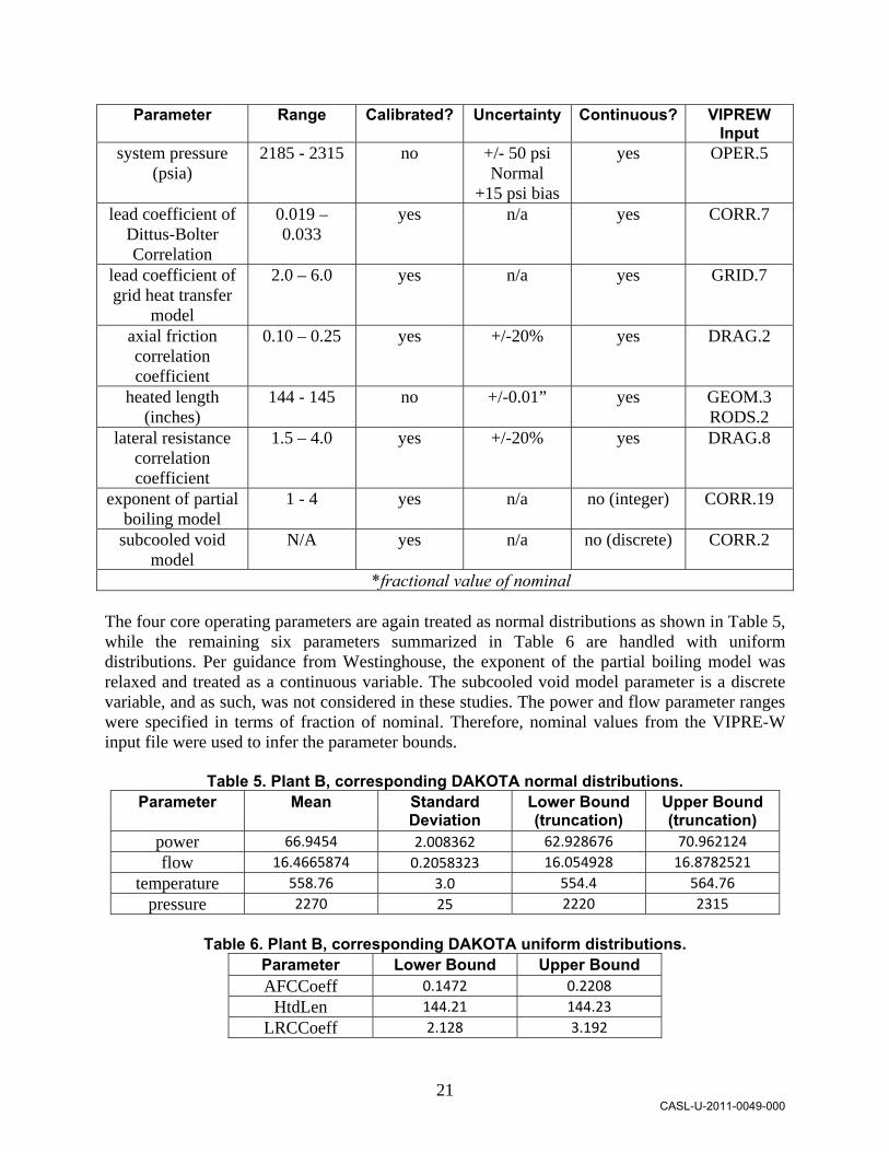
21

Parameter

Range Calibrated? Uncertainty Continuous? VIPREW Input

system pressure (psia)

2185 - 2315 no +/- 50 psi Normal

+15 psi bias

yes OPER.5

lead coefficient of Dittus-Bolter Correlation

0.019 – 0.033

yes n/a yes CORR.7

lead coefficient of grid heat transfer

model

2.0 – 6.0 yes n/a yes GRID.7

axial friction correlation coefficient

0.10 – 0.25 yes +/-20% yes DRAG.2

heated length (inches)

144 - 145 no +/-0.01” yes GEOM.3 RODS.2

lateral resistance correlation coefficient

1.5 – 4.0 yes +/-20% yes DRAG.8

exponent of partial boiling model

1 - 4 yes n/a no (integer) CORR.19

subcooled void model

N/A yes n/a no (discrete) CORR.2

*fractional value of nominal The four core operating parameters are again treated as normal distributions as shown in Table 5, while the remaining six parameters summarized in Table 6 are handled with uniform distributions. Per guidance from Westinghouse, the exponent of the partial boiling model was relaxed and treated as a continuous variable. The subcooled void model parameter is a discrete variable, and as such, was not considered in these studies. The power and flow parameter ranges were specified in terms of fraction of nominal. Therefore, nominal values from the VIPRE-W input file were used to infer the parameter bounds.

Table 5. Plant B, corresponding DAKOTA normal distributions. Parameter Mean Standard

Deviation Lower Bound (truncation)

Upper Bound (truncation)

power 66.9454 2.008362 62.928676 70.962124

flow 16.4665874 0.2058323 16.054928 16.8782521

temperature 558.76 3.0 554.4 564.76

pressure 2270 25 2220 2315

Table 6. Plant B, corresponding DAKOTA uniform distributions.

Parameter Lower Bound Upper Bound AFCCoeff 0.1472 0.2208

HtdLen 144.21 144.23

LRCCoeff 2.128 3.192

CASL-U-2011-0049-000

22

Parameter Lower Bound Upper Bound DBCoeff 0.019 0.033

GHTCoeff 2 6

ExpPBM 1 4

CASL-U-2011-0049-000

23

4. SENSITIVITY AND UNCERTAINTY RESULTS This section demonstrates sensitivity and uncertainty calculations for the two model problems. Recall that sensitivity studies are typically performed to understand how a system or model’s responses are related to its inputs. Such techniques can provide insight on how parameters are correlated and to what degree. These techniques are effective in screening and ranking model parameters to see which have significant influence on specific response quantities. An uncertainty analysis takes some understanding of the uncertainty in a model’s input parameters and maps it through to its responses, thereby, providing a distribution of possible response quantities. These can be used to answer questions like “What is the typical (mean) system response?” “What is its variability?” or “What is the probability of exceeding some critical response threshold?” Three different DAKOTA-provided techniques (Latin hypercube sampling (LHS), polynomial chaos expansion (PCE) and PSUADE’s Morris one-at-a-time (MOAT)), described in Section 2.3, were used to iteratively analyze the model relationships between system parameters and responses for both SA and UQ analyses. Samples of results from each technique are shown with conclusions in the following sections for both the Plant A and B models. The samples presented are not exhaustive, but rather representative of the kinds of results, analyses, and insights one can expect from these methods. Each of the SA and UQ techniques provides related, but slightly different information, as summarized in Table 7. The LHS option in DAKOTA provides moment-based statistics and 95% confidence intervals for each response function, and simple, partial, simple rank, and partial rank correlation matrices between input and output variables. The samples can also be exported to statistical software such as Minitab, SAS JMP, or Matlab for further analysis. The PCE option in DAKOTA reports the polynomial chaos coefficients for each response, along with estimated (both numerically and from the expansion) moment-based statistics for each response. Also, both local and global sensitivities as well as VBD Sobol’ indices are reported. MOAT provides the modified means and standard deviations of the elementary effects (EE) of each response variable with respect to each input parameter. The modified mean of the EE is a good indicator of a variable’s main effect, while the EE standard deviations indicate interaction or higher order effects for a particular input.

Table 7. Summary of SA and UQ metrics reported for each method type. Method Name Select Metrics for SA Select Metrics for UQ

LHS simple and partial correlation coefficients, scatter plots

mean, standard deviation

PCE Sobol’ indices (main and total effects of inputs) mean, standard deviation

MOAT modified mean and standard deviation of elementary effects

n/a

For each plant, four aggregate system response metrics were derived from output of each simulation run: maximum of the mass evaporation rate m-dot-e and mean of m-dot-e (each taken over all 193 channels and all 93 axial nodes), the number of nodes with nonzero m-dot-e (thus

CASL-U-2011-0049-000

24

indicating boiling), and the mean of m-dot-e taken strictly over the nonzero nodes. The associated response variable names used in DAKOTA are given in Table 8.

Table 8. DAKOTA response names corresponding to derived VIPRE-W system responses.

System Response Dakota Name m-dot-e, maximum ME_max

m-dot-e, mean ME_mean number nodes with

nonzero m-dot-e ME_nnz

m-dot-e, mean over nonzero nodes

ME_meannz

4.1. Results for Plant A This section summarizes exploratory studies conducted with DAKOTA and VIPRE-W for the Plant A model. A total of four uncertain parameters, treated as truncated, normally distributed variables as described in Section 3.1, were studied. 4.1.1. Comparison of Sensitivity Analysis Techniques The variable-response pairs resulting from a LHS study can be used to visually investigate the sensitivity relationship between inputs and outputs. Such analysis yields an expedient, if coarse, determination of if and how factors relate. Scatter plots between the input and response variables for the 400 sample LHS case are shown in Figure 3. (The plots were generated with Matlab using the DAKOTA-produced dakota_tabular.dat file, but can be generated with many readily available statistics software packages.) The scatter plots indicate a strong positive correlation between temperature and all four responses. They also demonstrate a weaker, inverse correlation between all responses and the pressure parameter. Omitted: Input-input scatter plots can also visually affirm that the input parameter sample sets look normally distributed within the parameter space as prescribed. DAKOTA also reports the input-input correlations of the sample set for verification purposes. Investigation of response-response inter-relationships revealed a nearly deterministic relationship between all response pairs. (ME_max, ME_meannz), and (ME_nnz, ME_mean) exhibited a strong linear relationship, whilst the other pairs showed clear non-linear relationships. This is likely an artifact of the derived metrics used in post-processing (smooth mean vs. truncation-like Boolean or max).

CASL-U-2011-0049-000

25

Figure 4. Matrix of scatter plots for parameters versus responses; based on the 400

sample LHS study of the Plant A model. The varying linear trends apparent in the visual analysis can be corroborated by correlation coefficients. The simple input-output correlation matrix for the 4000 sample case is shown in Table 9, which confirms the visually observed relationships. Temperature has the strongest linear effect; positively and highly correlated to all 4 responses (all above 0.75), whilst pressure is the second most influential parameter. It is slightly less strongly and inversely correlated to each of the responses (all approximately -0.5). The correlations between each of the responses was also strong (nearly unity) as was observed in the scatter plots (omitted for brevity).

Table 9. Simple correlations between inputs and outputs for Plant A, 4000 sample LHS analysis.

Response pressure temperature flow power ME_mean ‐0.503 0.763 ‐0.294 0.094

ME_nnz ‐0.540 0.766 ‐0.289 0.089

ME_meannz ‐0.464 0.812 ‐0.323 0.112

ME_max ‐0.464 0.806 ‐0.316 0.117

Table 10 summarizes the partial correlation coefficients, which can adjust for the effects of other variables. Here, temperature and pressure appear similarly influential, while flow is secondary.

Table 10. Partial Correlation Matrix for Plant A, 4000 Sample LHS Analysis.

Response pressure temperature flow power ME_mean ‐0.890 0.947 ‐0.749 0.344

ME_nnz ‐0.955 0.977 ‐0.863 0.472

ME_meannz ‐0.985 0.995 ‐0.969 0.811

ME_max ‐0.957 0.985 ‐0.913 0.644

CASL-U-2011-0049-000

26

Variable sensitivities and interactions can also be analyzed through use of polynomial chaos expansions, from which analytic Sobol’ indices can be computed. Table 11 is based on tensor-product PCE with increasing quadrature order and shows main and total effects for the ME_mean response. The main indices measure the effect of a parameter alone, whereas the total indices include interactions of the parameter with other factors. In this example, variability in ME_mean is again primarily influenced by temperature and secondarily by pressure. The 3rd order quadrature seemed adequate for converged statistics. DAKOTA reports these Sobol’ sensitivity indices for each response with respect to each input variable and each of the possible variable combinations; all interaction terms were insignificant and therefore not reported.

Table 11. PCE-based Sobol’ Indices for Plant A ME_mean response.

Variable

2nd Order Quadrature

3rd Order Quadrature

4th Order Quadrature

(16 evaluations) (81 evaluations) (256 evaluations) Main Total Main Total Main Total

pressure 2.670e‐01 2.975e‐01 2.626e‐01 2.922e‐01 2.625e‐01 2.921e‐01

temperature 5.960e‐01 6.317e‐01 6.052e‐01 6.397e‐01 6.054e‐01 6.399e‐01

flow 8.787e‐02 9.936e‐02 8.480e‐02 9.592e‐02 8.467e‐02 9.582e‐02

power 9.596e‐03 1.101e‐02 9.130e‐03 1.049e‐02 9.115e‐03 1.049e‐02

Table 12 provides the Sobol’ indices for all four responses for the 3rd order quadrature case. Temperature was consistently the most influential input parameter to all four responses with pressure as the second most influential. The results are relatively (though not entirely) insensitive to the choice of derived response metric.

Table 12. 3rd order PCE-based Sobol’ indices for all Plant A responses.

Variable ME_mean ME_nnz ME_meannz ME_max

Main Total Main Total Main Total Main Total pressure 2.626e‐01 2.922e‐01 2.975e‐01 3.113e‐01 2.147e‐01 2.193e‐01 2.170e‐01 2.272e‐01temperature 6.052e‐01 6.397e‐01 5.978e‐01 6.128e‐01 6.576e‐01 6.620e‐01 6.560e‐01 6.676e‐01

flow 8.480e‐02 9.592e‐02 8.044e‐02 8.477e‐02 1.079e‐01 1.101e‐01 9.995e‐02 1.044e‐01

power 9.130e‐03 1.050e‐02 7.586e‐03 7.967e‐03 1.431e‐02 1.470e‐02 1.379e‐02 1.419e‐02

The PSUADE MOAT results for the 4000 sample case are given in Table 13. These results support earlier conclusions that temperature is a dominant factor, while pressure is a secondary influence. There are no significant outliers in terms of elementary effect standard deviations, though indication of nonlinear or interaction effects roughly increases across power, through flow and pressure, to temperature. The results differ depending on the response metric considered; this method does not scale responses, so care is needed when interpreting. Figure 5 plots the modified mean versus the standard deviations of the elementary effects for each of the four parameters. This visual representation is often a useful diagnostic for identifying clusters of variables with minimal, linear, or higher-order effects, but here we observed that the most influential factors also have the highest variability in their influence throughout the parameter space.

CASL-U-2011-0049-000

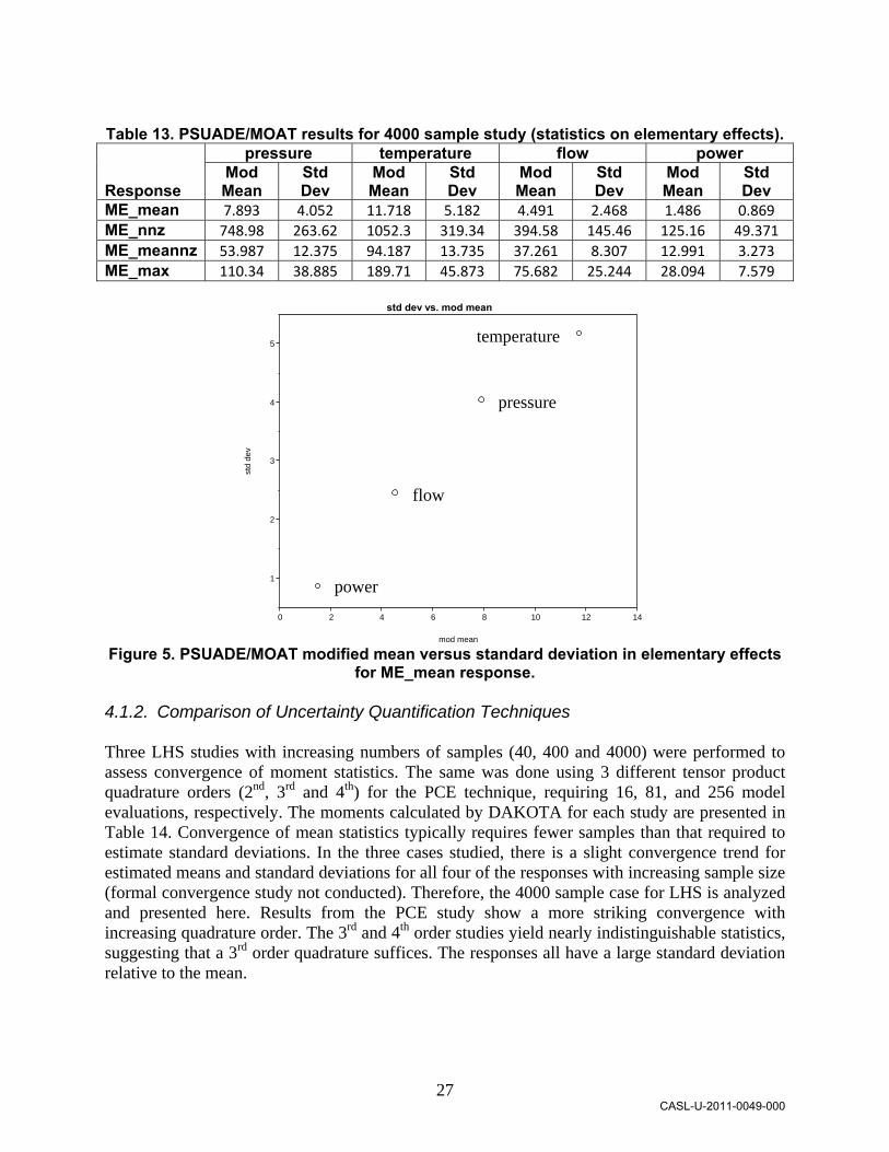
27

Table 13. PSUADE/MOAT results for 4000 sample study (statistics on elementary effects).

Response

pressure temperature flow power Mod Mean

Std Dev

Mod Mean

Std Dev

Mod Mean

Std Dev

Mod Mean

Std Dev

ME_mean 7.893 4.052 11.718 5.182 4.491 2.468 1.486 0.869

ME_nnz 748.98 263.62 1052.3 319.34 394.58 145.46 125.16 49.371

ME_meannz 53.987 12.375 94.187 13.735 37.261 8.307 12.991 3.273

ME_max 110.34 38.885 189.71 45.873 75.682 25.244 28.094 7.579

std dev vs. mod mean

mod mean

0 2 4 6 8 10 12 14

std

de

v

1

2

3

4

5

Figure 5. PSUADE/MOAT modified mean versus standard deviation in elementary effects

for ME_mean response. 4.1.2. Comparison of Uncertainty Quantification Techniques Three LHS studies with increasing numbers of samples (40, 400 and 4000) were performed to assess convergence of moment statistics. The same was done using 3 different tensor product quadrature orders (2nd, 3rd and 4th) for the PCE technique, requiring 16, 81, and 256 model evaluations, respectively. The moments calculated by DAKOTA for each study are presented in Table 14. Convergence of mean statistics typically requires fewer samples than that required to estimate standard deviations. In the three cases studied, there is a slight convergence trend for estimated means and standard deviations for all four of the responses with increasing sample size (formal convergence study not conducted). Therefore, the 4000 sample case for LHS is analyzed and presented here. Results from the PCE study show a more striking convergence with increasing quadrature order. The 3rd and 4th order studies yield nearly indistinguishable statistics, suggesting that a 3rd order quadrature suffices. The responses all have a large standard deviation relative to the mean.

temperature

pressure

power

flow

CASL-U-2011-0049-000

28

Table 14. Comparison of response means and standard deviations calculated by DAKOTA LHS and PCE methods for the Plant A model.

Method

ME_mean ME_nnz ME_meannz ME_max Mean Std

Dev Mean Std

Dev Mean Std

Dev Mean Std

Dev LHS (40) 5.069 3.263 651.225 297.039 127.836 27.723 361.204 55.862

LHS (400) 5.006 3.131 647.33 286.146 127.796 25.779 361.581 51.874

LHS (4000) 5.354 3.206 688.261 292.687 129.175 25.450 364.317 50.884

PCE (Θ(2)) 5.353 3.130 687.875 288.140 129.151 25.7015 364.366 50.315

PCE (Θ (3)) 5.355 3.202 688.083 292.974 129.231 25.3989 364.310 50.869

PCE (Θ (4)) 5.355 3.203 688.099 292.808 129.213 25.4491 364.313 50.872

Recall that the input parameters were characterized by normal distributions. The corresponding response (model output) distributions resulting from the UQ process are displayed in Figure 6. SAS JMP was used to analyze each response distribution to determine which analytical statistical distribution best fit the data. The results and data fits to each response are also shown in Figure 6. None of the response distributions are best fit by a normal distribution, underscoring the importance of not assuming normal inputs give rise to normally distributed model outputs. ME_mean and ME_nnz are best fit by Gamma distributions, whereas Weibull distributions best fit ME_meannz and ME_max. The validity of a normality assumption on the responses was assessed by a goodness of fit test. Figure 7 displays the test results for the ME_mean response, indicating that the output distribution is not normal.

0 10 20

Gamma(2.69973,1.98316,0)

MeanStd DevStd Err MeanUpper 95% MeanLower 95% MeanN

5.35398563.20593720.05069035.45336695.2546043

4000

Moments

ME_mean

0 1000 2000

Gamma(5.30746,129.678,0)


688.261292.687244.6277916697.33405679.18795

4000

Moments

ME_nnz

30 50 70 90 110 130 150 170 190

Weibull(139.442,5.82842)


129.1748925.4498820.402398

129.96381128.38596

4000

Moments

ME_meannz

200 300 400 500

Weibull(385.666,8.58881)


364.3166350.88351

0.8045389365.89398362.73929

4000

Moments

ME_max

Distributions

Figure 6. Plant A response distribution fits to analytical statistical distributions.

CASL-U-2011-0049-000

29

Figure 7. Goodness of fit test of normality on ME_mean.

4.2. Results for Plant B This section summarizes sensitivity and uncertainty studies conducted with DAKOTA and VIPRE-W for the Plant B model, which will be used in future calibration and validation activities. The investigation involved a total of ten parameters treated as either truncated, normally distributed or bounded, uniformly distributed variables, as described in Section 3.2. The system response metrics studied are as in the Plant A example. 4.2.1. Comparison of Sensitivity Analysis Techniques Figure 8 shows a scatter plot matrix of the 4 response variables against the 10 input variables, with linear regression lines superimposed. Overall the trends are less striking than for Plant A, perhaps due to the new model form variables dominating the analysis. The DBCoeff (lead coefficient of the Dittus-Bolter correlation) has the clearest influence, while the four reactor operating parameters again exhibit some correlation to the responses (see linear regression lines). The m-dot-e means over non-zeros and maximum both exhibit strong trend with the exponent of the partial boiling model (ExpPBM).

CASL-U-2011-0049-000

30

Figure 8. Scatter plots of inputs versus responses for Plant B, LHS 1000 samples.

The correlation data summarized in Table 15 give more insight into inter-variable relationships potentially difficult to characterize visually. The most influential parameter is confirmed as DBCoeff, which has a strong negative correlation (around -0.7 for simple and -0.9 for controlled partial correlation) with all four responses (also visible in the scatter plots). Westinghouse affirmed that the boiling surface is highly sensitive to this coefficient. Considering the partial correlations, temperature, power, and ExpPBM are the next most influential inputs. These correlations can be harder to discern directly from scatter plots.

Table 15. Correlations for Plant B 1000 sample LHS analysis.


simple partial simple partial simple partial simple partial pressure ‐0.167 ‐0.306 ‐0.217 ‐0.509 ‐0.152 ‐0.404 ‐0.166 ‐0.450

temperature 0.304 0.512 0.343 0.691 0.294 0.658 0.301 0.683

flow ‐0.111 ‐0.214 ‐0.126 ‐0.336 ‐0.133 ‐0.368 ‐0.142 ‐0.403

power 0.329 0.534 0.355 0.693 0.343 0.705 0.357 0.735

AFCCoeff ‐0.038 ‐0.066 ‐0.028 ‐0.067 ‐0.015 ‐0.027 ‐0.016 ‐0.031

HtdLen ‐0.013 ‐0.031 ‐0.013 ‐0.044 0.003 0.003 0.009 0.021

LRCCoeff ‐0.010 0.005 ‐0.005 0.020 ‐0.016 ‐0.003 ‐0.012 0.009

DBCoeff ‐0.662 ‐0.789 ‐0.743 ‐0.898 ‐0.704 ‐0.900 ‐0.688 ‐0.904

GHTCoeff ‐0.025 ‐0.045 ‐0.055 ‐0.147 0.010 0.041 ‐0.017 ‐0.041

ExpPBM 0.226 0.394 0.021 0.043 0.378 0.739 0.393 0.766

CASL-U-2011-0049-000

31

Sobol’ indices derived from PCE yield similar conclusions to the LHS studies. Table 16 shows the main and total effect indices for the ME_mean response for 2nd and 3rd order sparse grid quadrature, whereas Table 17 focuses on the 3rd order case, showing the main and total effects for all responses. In all cases, the DBCoeff is the most sensitive parameters, with temperature, power, and ExpPBM playing crucial secondary roles. Again, the parameter interactions are reported in the DAKOTA results file, but were all small, so are omitted. The absence of any strong interactions suggests that for these parameters, performing sensitivity analysis with a modest number of samples might suffice.

Table 16. PCE Sobol’ indices for ME_mean response for varying quadrature order.

Variable

2nd Order Quadrature 3rd Order Quadrature 327 Evaluations 2987 Evaluations Main Total Main Total

pressure 2.062e‐02 4.268e‐02 3.164e‐02 5.218e‐02

temperature 8.217e‐02 1.442e‐01 9.305e‐02 1.515e‐01

flow 1.012e‐02 2.261e‐02 1.710e‐02 2.868e‐02

power 1.012e‐01 1.768e‐01 1.051e‐01 1.773e‐01

AFCCoeff 1.975e‐04 5.102e‐04 4.877e‐04 7.460e‐04

HtdLen 1.691e‐07 4.121e‐07 2.883e‐07 5.153e‐07

LRCCoeff 1.709e‐07 4.225e‐07 8.986e‐06 5.152e‐05

DBCoeff 5.361e‐01 6.881e‐01 5.118e‐01 6.617e‐01

GHTCoeff 4.589e‐03 1.012e‐02 4.562e‐03 1.218e‐02

ExpPBM 5.032e‐02 1.097e‐01 4.834e‐02 1.141e‐01

Table 17. Sobol’ indices for all responses, 3rd order quadrature PCE case.


Main Total Main Total Main Total Main Total pressure 3.164e‐02 5.218e‐02 3.805e‐02 6.435e‐02 4.034e‐02 9.328e‐02 1.305e‐02 5.330e‐02temperature 9.305e‐02 1.515e‐01 1.413e‐01 1.852e‐01 7.856e‐02 1.621e‐01 1.205e‐01 1.840e‐01

flow 1.710e‐02 2.868e‐02 1.598e‐02 2.947e‐02 3.040e‐02 6.314e‐02 5.128e‐03 3.120e‐02

power 1.051e‐01 1.773e‐01 1.471e‐01 1.919e‐01 5.575e‐02 1.401e‐01 1.060e‐01 1.760e‐01

AFCCoeff 4.877e‐04 7.460e‐04 1.380e‐04 2.271e‐03 5.960e‐03 1.484e‐02 1.010e‐04 1.131e‐03

HtdLen 2.883e‐07 5.153e‐07 1.593e‐05 8.118e‐05 1.192e‐04 4.575e‐04 6.168e‐09 7.408e‐07LRCCoeff 8.986e‐06 5.152e‐05 4.245e‐06 6.408e‐05 2.273e‐04 7.139e‐04 1.059e‐06 5.274e‐06

DBCoeff 5.118e‐01 6.617e‐01 5.548e‐01 6.175e‐01 4.397e‐01 5.743e‐01 4.353e‐01 5.368e‐01

GHTCoeff 4.562e‐03 1.218e‐02 5.686e‐03 1.299e‐02 1.722e‐03 1.273e‐02 9.058e‐04 5.740e‐03

ExpPBM 4.834e‐02 1.141e‐01 2.298e‐08 3.608e‐07 1.288e‐01 2.015e‐01 1.680e‐01 2.193e‐01

The MOAT modified mean and standard deviation of elementary effects are shown in Table 18. Similar conclusions arise from them, but Figure 9 gives a different perspective on the data. It plots the elementary effects summaries for the ME_max response to demonstrate a potential advantage of the MOAT method (though one that is also enabled by nonlinear regression approaches). In indicates that DBCoeff mainly has a linear or additive effect, while ExpPBM, power, and temperature have effects that deviate considerably from the mean effect in different regions of the input parameter space. Pressure and flow have both main and interaction effects, but of smaller magnitude.

CASL-U-2011-0049-000

32

Table 18. Plant B summary of elementary effects based on 990 MOAT evaluations.

Variable

ME_mean ME_nnz ME_meannz ME_max Mod Mean

Std Dev

Mod Mean

Std Dev

Mod Mean

Std Dev

Mod Mean

Std Dev

pressure 6.554 6.589 478.90 366.22 53.147 53.576 100.93 99.345

temperature 12.594 11.717 815.23 542.05 104.26 87.435 209.01 178.18

Flow 5.346 5.532 355.77 272.51 35.249 35.486 68.966 66.255

Power 12.373 12.918 799.61 589.10 125.98 95.106 271.71 196.33

AFCCoeff 0.514 0.455 27.028 18.764 6.063 5.994 8.895 9.073

HtdLen 0.0168 0.0168 1.128 1.722 0.334 0.489 0.287 0.244

LRCCoeff 0.0719 0.197 3.150 6.338 1.005 2.525 0.442 1.315

DBCoeff 20.411 19.135 1314.5 844.56 213.17 132.71 412.33 255.43

GHTCoeff 2.802 3.526 180.66 174.35 7.120 9.788 8.464 21.159

ExpPBM 8.845 12.625 0.117 0.519 133.7 122.57 234.34 200.00

0 50 100 150 200 250 300 350 400 450

0

20

40

60

80

100

120

140

160

180

200

pressure

temperature

flow

power

AFCCoeff

DBCoeff

GHTCoeff

ExpPBM

modified mean of EE

sta

nd

ard

de

via

tio

n o

f E

E

Figure 9. Plant B: MOAT statistics for ME_max response based on 990 model

evaluations. 4.2.2. Comparison of Uncertainty Quantification Techniques LHS and PCE methods propagated the uncertainties identified in Section 3.2. Sample sizes of 100, 1000, and 10000 (10x, 100x, and 1000x the number of variables) were used with the LHS method. Sparse grid quadrature rules with orders 2 and 3 were used with PCE, requiring 327 and 2987 model evaluations, respectively. PCE with 4th order quadrature runs did not finish in time to be included. Per Table 19, the means of the responses are similar to those for Plant A (Table 14), however the estimated variability (reported by standard deviation) is considerably larger. In many cases, it is

CASL-U-2011-0049-000

33

nearly the same magnitude as the mean value. This is likely a reflection of a large amount of uncertainty due to the model form parameters considered in this study. Should these predictions of uncertainty be unacceptably high, a decision should be made whether to better characterize them, reducing uncertainty, or consider them fixed parameters for a given analysis (or possibly treat them as epistemic uncertainties). As many of these parameters are likely to be calibrated to data, it is possible their uncertain range could be substantially reduced.

Table 19. Comparison of Response Means and Standard Deviations Using Different UQ Techniques for Plant B Model

Method ME_mean ME_nnz ME_meannz ME_max

Mean Std Dev Mean Std Dev Mean Std Dev Mean Std DevLHS(100) 5.919 7.822 485.020 463.892 140.776 102.468 311.099 199.434

LHS(1000) 5.865 7.911 480.552 467.080 138.975 103.708 305.296 200.135

LHS(10000) 5.848 7.719 481.643 464.996 139.114 102.983 304.626 199.451

PCE(Θ(2)) 5.894 7.718 517.556 470.024 130.199 111.855 309.373 201.172

PCE(Θ(3)) 5.830 7.713 455.964 480.917 151.293 109.538 304.074 213.559

Figure 10 shows that the response distributions for Plant B differ substantially from those for Plant A, with most exhibiting a more exponential character. The probability mass near zero is a potential concern, as it may indicate simulation failures over some of the parameter ranges. Examination of the individual LHS samples revealed that many scenarios sampled exhibited no boiling. Further discussion with Westinghouse is needed on this issue. Figure 11 again rejects the hypothesis that the response data come from a normal distribution. A follow on UQ study is likely warranted, considering a more plausible range on the calibration parameters related to model form.

CASL-U-2011-0049-000

34

0 10 20 30 40 50 60

Johnson Sl(0.34346,0.01342,-2e-103,1)


5.86504837.91125540.25017596.35597885.3741178

1000

Moments

Show

Johnson SlJohnson SuGLogExponentialNormal

Distribution

34312

Number of

Parameters

-39733.384-27720.9143801.493445538.021446973.45002

-2*LogLikelihood

-39727.36-27712.8743807.517535540.025456977.46205

AICc

Compare Distributions

ME_mean

0 1000 2000 3000

Exponential(480.552)


480.552467.0804614.770381509.53653451.56747

1000

Moments

Show

ExponentialJohnson SlJohnson SuGLogNormal

Distribution

13432

Number of

Parameters

14349.870914601.681314601.681314742.729915129.8801

-2*LogLikelihood

14351.874914607.705414609.7215

14748.75415133.8922

AICc


ME_nnz

0 100 200 300 400

Exponential(138.976)


138.97556103.70832

3.279545145.41115132.53997

1000

Moments

Show

ExponentialJohnson SlGLogNormalJohnson Su

Distribution

13324

Number of

Parameters

11868.596212040.405112103.225912120.041712120.0508

-2*LogLikelihood

11870.600212046.4292

12109.2512124.0538

12128.091

AICc


ME_meannz

0 100 200 300 400 500 600 700

Normal(305.296,200.135)


305.2955200.13508

6.328827317.71482292.87618

1000

Moments

Show

NormalJohnson SlGLogJohnson SuExponential

Distribution

23341

Number of

Parameters

13434.862213434.384613434.8646

13434.86813442.5603

-2*LogLikelihood

13438.874213440.408713440.888713442.908213444.5643

AICc


ME_max

Distributions

Figure 10. Best-fit distributions for Plant B outputs, based on 1000 LHS samples.

CASL-U-2011-0049-000

35

Figure 11. Test for normality of response ME_max for Plant B, based on 1000 samples.

Figure 12 and Figure 13 depict the mean of mass evaporation rate at each computational node in the simulation in 3D and overhead views, respectively (based on 100 LHS samples). Even these crude graphics demonstrate that there is considerable variation in m-dot-e at various locations in the reactor quarter core. Figure 14 and Figure 15 show similar plots, but instead for the standard deviation of m-dot-e at each node in the simulation. Again, variability across the domain is striking, and the areas of high variability do not necessarily correspond to areas of high mean performance.

CASL-U-2011-0049-000

36

Figure 12. Plot of mean of mass evaporation rate (taken over 100 LHS samples) at each

node in the Plant B computational model.

Figure 13. Plot of mean of mass evaporation rate viewed from above the Plant B core.

CASL-U-2011-0049-000

37

Figure 14. Plot of standard deviation of mass evaporation rate (taken over 100 LHS

samples) at each node in the Plant B computational model.

Figure 15. Plot of standard deviation of mass evaporation rate viewed from above the

Plant B core.

CASL-U-2011-0049-000

38

CASL-U-2011-0049-000

39

5. DISCUSSION This VUQ milestone demonstrated statistical sensitivity and uncertainty quantification using VERA tools (VIPRE-W and DAKOTA) on PWR problems of interest to the AMA focus area. The tools were used to assess response metrics predictive of CIPS. While conducted with loose-coupled simulation tools, similar studies will soon be conducted leveraging tightly integrated executables based on DAKOTA/LIME integration. For Plant A, the three SA techniques applied consistently rank temperature as the most influential parameter and pressure as second. Temperature exhibits positive correlation while pressure is negatively correlated. In follow-on studies, it might be possible to neglect the effect of power as it has comparably minimal effect on m-dot-e. As the VIPRE-W model appears to behave relatively linearly and smoothly with respect to these parameters, only a small number of model evaluations should typically be needed to make these sensitivity assessments. The sensitivity analysis for Plant B better demonstrates the power of these screening techniques. Here, the lead coefficient of the Dittus-Bolter correlation and the exponent of the partial boiling model are crucial model form parameters and the four operating parameters are again significant factors. However, the remaining model form parameters (due to be calibrated) have comparably little effect. In the uncertainty quantification studies, both LHS and PCE techniques yielded similar estimates for the response means and standard deviations. (In some scenarios, PCE could provide considerable cost savings over Monte Carlo methods to obtain similar results, though for high dimensional parameter spaces sampling may prove more effective). Considerable Plant B variability is likely attributable to model form parameters ExpPBM and DBCoeff; some consideration should be given to whether they should be considered in performing forward propagation of uncertainty. Simulation results indicate considerable variation in both mean and standard deviation of m-dot-e throughout the reactor quarter core. Better visualization tools would likely help make this information useful to engineering analysts. The studies conducted illustrate the kinds of algorithms available through DAKOTA for SA and UQ, the assumptions they make and input characterization they require, and the kinds of insights they can offer. The results presented are not exhaustive, but rather presented for purposes of capability demonstration in fulfillment of this milestone. The study demonstrated a VUQ workflow and process that could be used with other multi-physics code systems for evaluating challenge problems for operating reactors.

CASL-U-2011-0049-000

40

CASL-U-2011-0049-000

41

6. REFERENCES 1. Stewart, C.W., Cuta, J.M., Montgomery, S.D., Kelly, J.M., Basehore, K.L., George, T.L.,

Rowe, D.S., VIPRE-01: A thermal-hydraulic code for reactor cores, Volumes 1—3 (Revision 3, August 1989) and Volume 4 (April 1987), NP-2511-CCM-A, Electric Power Research Institute.

2. Secker, J.R., Young, M.Y., Sung, Y., Lider, S., Johansen, B.J., BOB: An integrated model

for predicting axial offset anomaly, TOPFUEL Conference, Sweden, 2001. 3. Karoutas, Z.E., Sung, Y., Chang, Y., Kogan, G., Joffre, P., Subcooled boiling data from rod

bundles, TR1003383, Electric Power Research Institute, September 2002. 4. Sabol, G.P., Secker, J.R., Kormuth, J., Kunishi, H., Nuhfer, D.L., Rootcause investigation of

axial power offset anomaly, TR-108320, Electric Power Research Institute, June 1997. 5. Adams, B.M., Bohnhoff, W.J., Dalbey, K.R., Eddy, J.P., Eldred, M.S., Gay, D.M., Haskell,

K., Hough, P.D., and Swiler, L.P., DAKOTA, A Multilevel Parallel Object-Oriented Framework for Design Optimization, Parameter Estimation, Uncertainty Quantification, and Sensitivity Analysis: Version 5.0 User's Manual, Sandia Technical Report SAND2010-2183, December 2009. Updated December 2010 (Version 5.1).

6. A. Saltelli, Sensitivity analysis in practice: a guide to assessing scientific models, John

Wiley & Sons, Inc., 2004. 7. L.P. Swiler and G.D. Wyss, A user’s guide to Sandia’s Latin hypercube sampling software:

LHS UNIX library and standalone version, Sandia Technical Report SAND04-2439, Sandia National Laboratories, Albuquerque, NM, July 2004.

8. C. Storlie, L. Swiler, J. Helton, and C. Sallaberry, Implementation and evaluation of

nonparametric regression procedures for sensitivity analysis of computationally demanding models, Reliability Engineering and System Safety, 94 (2009), pp. 1735–1763.

9. A. Saltelli, K. Chan, and E. Scott, eds., Sensitivity analysis, John Wiley & Sons, Inc., 2000. 10. A.A. Giunta, J.M. McFarland, L.P. Swiler, and M.S. Eldred, The promise and peril of

uncertainty quantification using response surface approximations, Structure and Infrastructure Engineering, 2 (2006), pp. 175–189.

11. M.S. Eldred, C.G. Webster, and P. Constantine, Evaluation of non-intrusive approaches for

Wiener-Askey generalized polynomial chaos, in Proc. 10th AIAA Non-Deterministic Approaches Conference, AIAA-2008-1892, Schaumburg, IL, April 7–10, 2008.

12. B. Sudret, Global sensitivity analysis using polynomial chaos expansions, Reliability

Engineering & System Safety, 93 (2008), pp. 964—979.

CASL-U-2011-0049-000

42

13. G. Tang, G. Iaccarino, and M. Eldred, Global sensitivity analysis for stochastic collocation expansion, in Proc. 51st AIAA/ASME/ASCE/AHS/ASC Structures, Structural Dynamics, and Materials Conference (12th AIAA Non-Deterministic Approaches Conference), AIAA-2010-2922, Orlando, FL, April 2010.

14. M.D. Morris. Factorial sampling plans for preliminary computational experiments.

Technometrics, 33 (1991), pp. 161–174.

CASL-U-2011-0049-000

43

APPENDIX A: SAMPLE ANALYSIS FILES

Figure 16. Representative DAKOTA input file for performing Latin hypercube sampling

for Plant A.

strategy, single_method tabular_graphics_data method, nond_sampling samples = 4000 seed = 17 sample_type lhs model, single variables, normal_uncertain = 4 # nominal: 2270.0, 556.4, 15.93387, 67.88742 # bias: 20.0, 1.0 # uncert: 50.0, 5.0, 2%, 0.6% means 2270.0 556.4 15.93387 67.88742 std_deviations 25.0 2.5 0.1593387 0.20366226 lower_bounds 2220.0 551.4 15.6151926 67.48009548 upper_bounds 2320.0 561.4 16.2525474 68.29474452 descriptors 'pressure' 'temperature' 'flow' 'power' interface, fork analysis_driver = 'runvipre_massevap.sh' asynchronous evaluation_concurrency = 2 work_directory named 'workdir' directory_tag directory_save file_save template_files = 'wat7_epri.5806.inp.template' copy parameters_file = 'params.in' results_file = 'results.out' responses, num_response_functions = 4 descriptors = 'ME_mean' 'ME_nnz' 'ME_meannz' 'ME_max' no_gradients no_hessians

CASL-U-2011-0049-000

44

Figure 17. Shell script runvipre_massevap.sh iteratively called by DAKOTA.

#!/bin/sh # pre‐process with dprepro ../dprepro.formatted params.in wat7_epri.5806.inp.template wat7_epri.5806.inp # run vipre R711.odin wat7_epri.5806.inp # post‐process massevap_stats.sh wat7_epri.5806.inp.out results.out

CASL-U-2011-0049-000

45

Figure 18. Shell script massevap_stats.sh used to post-process VIPRE-W output to

generate metrics of interest for return to DAKOTA.

#!/bin/sh infile=$1 if [ $# ‐gt 1 ]; then outfile=$2 else outfile="default.stats" fi # channel axial axial mass evap local heat flux components local # number node height rate forced conv nuc boil boil incept pressure # inches lbm/hr‐ft2 <‐‐‐ MBTU/hr‐ft2 ‐‐‐> psia # there are # 193 channels # 93 axial nodes # each header is followed by data for each of 93 axial nodes grep ‐A 96 "mass evap" $infile | egrep "^[ ]+[0‐9]+" > wat7.5806.massevap.dat rows=`wc ‐l wat7.5806.massevap.dat | cut ‐f1 ‐d' '` if [ $rows ‐eq 17949 ]; then echo "Mass evaporation data has correct number of rows." else echo "WARNING: possible wrong number of rows in Mass evaporation data" fi # calculate mean of mass evaporation rate (column 4) massevap_mean=àwk 'BEGIN {sum=0.0 } {sum += $4} END {printf "%20f", sum/NR}' wat7.5806.massevap.dat` # calculate number of nodes in boiling massevap_nnz=àwk 'BEGIN {nnz=0; sum=0.0} {if ($4 > 0.0) nnz +=1; sum+=$4 } END {printf "%20d", nnz}' wat7.5806.massevap.dat` # calculate average over non‐zero nodes massevap_mean_nz=àwk 'BEGIN {nnz=0; sum=0.0} {if ($4 > 0.0) nnz +=1; sum+=$4 } END {printf "%20f", sum/nnz}' wat7.5806.massevap.dat` # calculate max massevap_max=àwk 'BEGIN {max=0.0} {if ($4 > max) max=$4 } END {printf "%20f", max}' wat7.5806.massevap.dat` echo "$massevap_mean ME_mean" > $outfile echo "$massevap_nnz ME_nnz" >> $outfile echo "$massevap_mean_nz ME_meannz" >> $outfile echo "$massevap_max ME_max" >> $outfile

CASL-U-2011-0049-000

46

DISTRIBUTION 1 MS0899 Technical Library 9536 (electronic copy)

CASL-U-2011-0049-000

47

CASL-U-2011-0049-000

CASL-U-2011-0049-000

l2:vuq.p2.03 brian adams snl completed: 3/31/11 · software tools, characterizing uncertainties,...

Documents