lab 11: free damped and forced...

Lab 11 – Free, Damped, and Forced Oscillations 129

Name__________________________Date___________________Partner______________________________

LAB 11: FREE, DAMPED, AND FORCED OSCILLATIONS

OBJECTIVES

• To understand the free oscillations of a mass and spring.

• To understand how energy is shared between potential and kinetic energy.

• To understand the effects of damping on oscillatory motion.

• To understand how forced oscillations dominates oscillatory motion.

• To understand the effects of resonance in oscillatory motion. OVERVIEW You have already studied the motion of a mass moving on the end of a spring. We understand that the concept of mechanical energy applies and the energy is shared back and forth between the potential and kinetic energy. We know how to find the angular frequency of the mass motion if we know the spring constant. We will examine in this lab the mass-spring system again, but this time we will have two springs - each having one end fixed on either side of the mass. We will let the mass slide on an air track that has very little friction. We first will study the free oscillation of this system. Then we will use magnets to add some damping and study the motion as a function of the damping coefficient. Finally, we will hook up a motor that will oscillate the system at practically any frequency we choose. We will find that this motion leads to several interesting results including wildly moving resonance. Harmonic motions are ubiquitous in physics and engineering; We observe them in mechanical and electrical systems. The same general principles apply for atomic, molecular, and other oscillators, so once you understand harmonic motion in one guise you have the basis for understanding an immense range of phenomena. An example of a simple harmonic oscillator is a mass m which moves on the x-axis and is attached to a spring with its equilibrium position at x = 0. When the mass is moved from its equilibrium position, the restoring force of the spring tends to bring it back to x = 0. The spring force is given by

,springF kx= − (1)

where k is the spring constant. The equation of motion for m becomes

2

2

d xm

dtkx= − (2)

This is the equation for simple harmonic motion. Its solutions are sine and cosine functions, as one can easily verify:

1 2 sin and cos .x A t x B tω ω= = (3)

University of Virginia Physics Department PHYS 142W, Spring 2004

130 Lab 11 – Free, Damped, and Forced Oscillations

The theory of linear differential equations tells us that when x1 and x2 are solutions, x = x1 + x2 is also a solution. Therefore we may write

0sin cos .0 x A t Bω= + tω (4) where

0

km

ω = (4a)

A and B are constants of integration; they are determined by the initial conditions. For instance, if at t = 0, x = 0, we find that B must be equal to zero. A may be determined from the value of dx/dt at t = 0.

Equation (4) can be rewritten in the following way:

0 0sin cos B

x A tA

ω ω= +

t

Set tan :BA

δ=

( )0 0cos sin sin cos cos

Ax t tδ ω δ ω

δ= +

or, set A/(cos δ) = A' and use a trigonometric identity to obtain:

x = A' sin (ω 0t + δ)

This expression is simpler to use; δ is the phase difference between this oscillation and an ordinary sine wave. If we assume δ = 0, then

sin ox A tω=

We can calculate the velocity by differentiating with respect to time:

0 0 cos dx

v Adt

tω ω= =

The kinetic energy is

2 22 2 20

0

1. . cos cos

2 2 2 o

m A kK E mv t A t

ω 2ω ω= = =

The potential energy is given by integrating the force on the spring times the displacement:

( )2

2 200

1. . sin

2 2x kA

P E kx dx kx tω= + = =∫

We see that the sum of the two energies is constant:

2

. . . .2

kAK E P E+ =

This constant is the potential energy at an extreme position of the mass, where v = 0.



INVESTIGATION 1: FREE OSCILLATIONS We have already studied the free oscillations of a spring in a previous lab, but let's quickly determine the spring constants of the two springs that we have. To perform this laboratory you will need the following equipment:

• force probe • motion detector

• mechanical vibrator • air track and cart glider

• two springs with approximately equal spring constants

• electronic balance • four ceramic magnets

• masking tape • string with loops at each end, ~30 cm long Activity 1-1: Measuring the Spring Constant To determine the spring constant, we shall use the method that we used in Lab 8. Because F = -kx, we can use the force probe to measure the force on the spring F and the motion detector to measure the corresponding spring stretching x. 1. Turn on the air supply for the air track. Make sure the air track is level. Check it by placing the

glider on the track and see if it is motionless. Some adjustments may be necessary on the feet, but be careful, because it may not be possible to have the track level over its entire length.

2. Tape four ceramic magnets to the top of the glider cart and measure the mass of the glider cart on

the electronic balance.

glider cart mass _______________ kg (with four magnets) 3. Never move items on the air track unless the air is flowing! You might scratch the surfaces

and create considerable friction. Set up the force probe, glider, spring, motion detector, and mechanical vibrator as shown below on the air track. If not already done, tie a loop at each end of a string, so that it ends up about 30 cm long. Loop one end around the force probe hook and the other end around the metal flag on the glider cart. Note the spring you put on the apparatus as spring 1. Make sure the mechanical vibrator-oscillator driver is in the locked position.

4. Op

5. Ze 6. Pu 7. St

so

UniverPHYS

Flag Motion detector Mechanical vibrator Spring Force Glider probe

en the experiment file called Spring Constant L11.1-1.

ro the force probe with no force on it.

ll the mechanical vibrator back slowly until the spring is barely extended.

art the computer and begin graphing. Use your hand to slowly pull the mechanical vibrator that the spring is extended about 30 cm. Hold the vibrator still and stop the computer.

sity of Virginia Physics Department 142W, Spring 2004


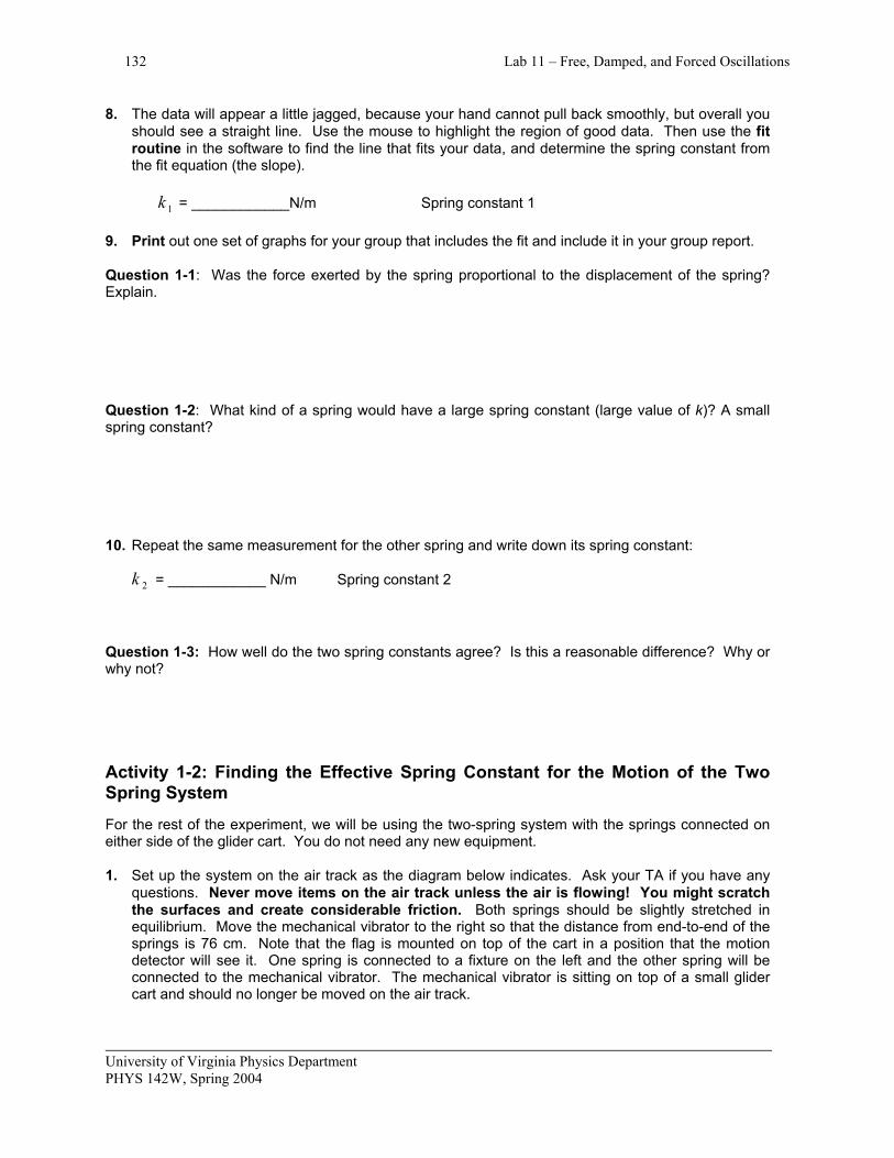
8. The data will appear a little jagged, because your hand cannot pull back smoothly, but overall you should see a straight line. Use the mouse to highlight the region of good data. Then use the fit routine in the software to find the line that fits your data, and determine the spring constant from the fit equation (the slope).

k 1 = ____________N/m Spring constant 1 9. Print out one set of graphs for your group that includes the fit and include it in your group report. Question 1-1: Was the force exerted by the spring proportional to the displacement of the spring? Explain. Question 1-2: What kind of a spring would have a large spring constant (large value of k)? A small spring constant? 10. Repeat the same measurement for the other spring and write down its spring constant:

k = ____________ N/m Spring constant 2 2

Question 1-3: How well do the two spring constants agree? Is this a reasonable difference? Why or why not? Activity 1-2: Finding the Effective Spring Constant for the Motion of the Two Spring System For the rest of the experiment, we will be using the two-spring system with the springs connected on either side of the glider cart. You do not need any new equipment. 1. Set up the system on the air track as the diagram below indicates. Ask your TA if you have any

questions. Never move items on the air track unless the air is flowing! You might scratch the surfaces and create considerable friction. Both springs should be slightly stretched in equilibrium. Move the mechanical vibrator to the right so that the distance from end-to-end of the springs is 76 cm. Note that the flag is mounted on top of the cart in a position that the motion detector will see it. One spring is connected to a fixture on the left and the other spring will be connected to the mechanical vibrator. The mechanical vibrator is sitting on top of a small glider cart and should no longer be moved on the air track.



Force probe String Flag Motion detector Mechanical vibrator Spring 1 Spring 2 Fixed Glider cart end

2. You will continue to use the same experimental file used previously in Activity 1-1, Spring

Constant L11.1-1. Delete any data showing. 3. Make sure the air is on for the air track. A string is connected near the bottom of the flag on the

glider cart to the force probe. In this experiment you will be holding the force probe in your hand and pulling the force probe to the left.

4. Zero the force probe and hold on to the force probe. 5. Let a colleague start the computer taking data. When you hear the motion detector clicking (or

see the green light), start pulling the force probe slowly to the left about 10 cm or so. Spring 1 should still be extended. Stop the computer.

6. Do the same analysis that you did in Activity 1-1 to determine the spring constant of the

combined two-spring system.

Spring constant k ___________ N/m 7. Print out one graph with the linear fit showing and include with your group report. Question 1-4: How well does this value of the spring constant agree with the individual ones you found previously? Explain any differences you found. Question 1-5: What relationship exists between the effective spring constant for the two spring system and the individual spring constants? Activity 1-3: Free Motion of the Two Spring System Remove the force probe and string connected to the flag from the previous experiment. Now we want to examine the free oscillations of this system. 1. Open the experimental file Two Spring System L11.1-3. Delete any data showing.



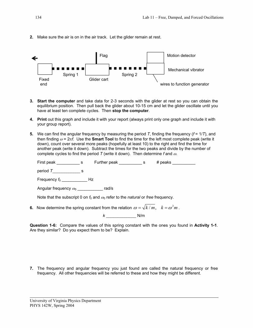
2. Make sure the air is on in the air track. Let the glider remain at rest.

Flag Motion detector Mechanical vibrator Spring 1 Spring 2 Fixed Glider cart end wires to function generator

3. Start the computer and take data for 2-3 seconds with the glider at rest so you can obtain the equilibrium position. Then pull back the glider about 10-15 cm and let the glider oscillate until you have at least ten complete cycles. Then stop the computer.

4. Print out this graph and include it with your report (always print only one graph and include it with

your group report).

5. We can find the angular frequency by measuring the period T, finding the frequency (f = 1/T), and then finding ω = 2πf. Use the Smart Tool to find the time for the left most complete peak (write it down), count over several more peaks (hopefully at least 10) to the right and find the time for another peak (write it down). Subtract the times for the two peaks and divide by the number of complete cycles to find the period T (write it down). Then determine f and ω.

First peak __________ s Further peak __________ s # peaks __________ period T____________ s Frequency f0 ___________ Hz Angular frequency ω0 ___________ rad/s Note that the subscript 0 on f0 and ω0 refer to the natural or free frequency.

6. Now determine the spring constant from the relation 2/ ,k m k mω ω= = .

k _____________ N/m Question 1-6: Compare the values of this spring constant with the ones you found in Activity 1-1. Are they similar? Do you expect them to be? Explain. 7. The frequency and angular frequency you just found are called the natural frequency or free

frequency. All other frequencies will be referred to these and how they might be different.



Question 1-7: Describe the motion that you observed in this activity. Does it look like it will continue for a long time? Did you observe any damping? Question 1-8: Does the motion in this activity look like it could be fit with a sinusoidal function offset from zero? INVESTIGATION 2: DAMPED OSCILLATORY MOTION Equation (2) in the previous section describes a periodic motion that will last forever. The only force acting on the mass is the restoring force .springF In practice one will also have friction. The general type of friction, which occurs between oiled surfaces, or in liquids and gases, is not constant but depends on the velocity. The simplest form is:

resistive friction (kinetic) = - k

dxf b

dt= (7)

The dry friction df Nµ= is also found in mechanical systems; but in electrical oscillations the

damping term is almost always of the form (7).

The new equation of motion becomes:

2

2 0

d x dxm b kx

dt dt+ + = (8)

A pure sine or cosine function will not satisfy this equation. We may guess a solution consisting of

a sine or cosine function with an amplitude which depends also on the time because the friction will cause the oscillation to damp down. A reasonable amplitude function will be a decreasing exponential

0tA A e α−= (9)

This amplitude will decrease by equal fractions in equal time differences:

(2

2 1

1

2 2

1 1

t

t tt

A e Aor e

A e A

αα

α

−− −

−= = ) (10)

Notice that only t2 - t1 = ∆t occurs and not the time itself. If we take the natural logarithm of both sides, we obtain

22 1ln ( )A t t

Aα

= − −

(11)



and α can be found from

2

1

2 1

ln

( )

AA

t tα

= − −

(12)

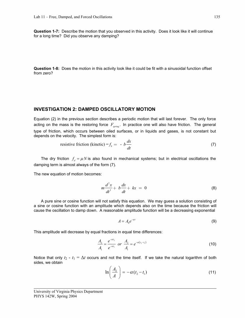
For instance, for A1/A2 = 1/2 we find

1ln(2) 0.693 / and 0.693/ .t tα

αα∆ = = = ∆ See Fig. 1.

1.0

0.5

0.25 0.125

α∆ t 0.693 2 (0.693) 3 (0.693)

Fig. 1 The function

0 sin tx A e tα ω−= (13)

is in fact a solution of equation (8): To verify this we evaluate

0 0sin cost tdxA e t A e

dtα α tα ω ω− −= − + ω

2

2 20 0 02

sin 2 cos sin t t td xA e t A e t A e

dtα α α tα ω α ω ω ω− − −= + − − ω

tα ω

=

Therefore, from Eq. (8),

2 - - - 2 -0 0 0 0sin - 2 cos - sin - sint t tmA e t mA e t mA e t bA e tα α αα ω α ω ω ω ω α

- -0 0cos sin 0t tbA e t kA e tα αω ω ω+ +

In this equation we may divide through by 0tA e α− after which we obtain an equation with sine and

cosine terms. We can only make this equation identically zero for arbitrary time if both the amplitude of the sine and of the cosine are equal to zero. Therefore:

2 2 - - m m b kα ω α + = 0 (14)



and -2 0m bαω ω+ = (15)

Equation (15) determines the damping term α,

2bm

α = (16)

and equation (14) the frequency ω, 2

2

1-

4k bm m

ω= (17)

To distinguish this angular frequency from the previous natural or free angular frequency ω0, let’s call the angular frequency in Equation (17) ωD for damping. Using Equation (16) for α, we can now write ωD as

20D

2ω ω α= − (18)

The complete solution is

2

0 2

-2 1

sin - 4

bm

t k bx A e t

m mδ=

+ (19)

A0 and δ are the constants of integration. It is evident that the frequency

2

2

1-

4k bm m

=ω (20)

has to be real. When (1/4) b2/m2 > k/m, the mass will not oscillate, and the solution will be a sum of two decreasing exponentials. The function for x, Equation (19), is sketched in Fig. 2

-1

-0.5

0

0.5

1

0 1 2 3 4 5 6 7 8 9 10

Am

plitu

de

Time (sec)

Fig. 2. Plot of A(t) = ( )10 te π− cos 2πt. The dashed lines are plots of the exponential factor.



The damping term is (1/2) b/m and the frequency ( ) 2 2- 1 4k m b mω = . Note that it is shifted from

the frequency 0 k mω = . For small damping one may neglect the shift. If the square root is equal to zero we call the system critically damped; no oscillations occur in that case. Shock absorbers in cars are so constructed that the damping is nearly critical. One does not increase the damping beyond critical because the ride would feel too hard. Most motions in nature do not have simple free oscillations like we had in the previous investigation. It is more likely there will be some kind of friction or resistance to damp out the free motion. In this investigation we will start the free oscillations like we did in the previous experiment, but we will add some damping. Air resistance is a good example of damping in nature. Automobile springs are damped (by shock absorbers) to reduce motion caused by cars running through ruts in the road, for example. We can add damping by attaching one or more strong ceramic magnets to the side of the moving cart. In your study of electromagnetism, you will learn that a moving magnetic field sets up a second magnetic field to oppose the effects of the original magnetic field. This is explained by Lenz's Law. The magnets we attach to the moving cart will cause magnetic fields to be created in the aluminum air track that will oppose the motion of the cart. The effect will be one of damping. The opposing magnetic fields are caused by induced currents, called eddy currents, and they will eventually dissipate in the aluminum track due to resistive losses. The motion carts themselves are made of non-magnetic material that allows the magnetic field to pass through (iron carts would not work). We can change the magnitude of this damping force by the number of magnets we attach. Activity 2-1: Description of Damped Harmonic Motion 1. Place a ceramic magnet symmetrically on each side of the glider cart, in the middle. Leave the

other magnets taped to the top of the cart so they will not damp out the motion. Use a small piece of tape to keep the magnets in place.

2. Open the experiment file called Spring Oscillations L11.2-1. 3. Make sure the air is on for the air track, the glider is at equilibrium and not moving on the air track. 4. Start the computer. Let the glider be at rest for a couple of seconds, so you can obtain the

equilibrium position. Then pull back the glider about 10 - 15 cm and release it. 5. Let the glider oscillate through at least ten cycles before stopping the computer. Note that the

oscillations have smaller and smaller amplitudes. This is due to the damping. Question 2-1: Does the motion seem to agree with Eq. (10) that was derived for this case? 6. Print out the graphs, but do not erase the data (keep this as Run 1). 7. Determine the angular frequency for damping ωD by using the period T for ten cycles.

Time for 10 cycles: ___________ s; Period T __________ s; Frequency fD ___________ Hz. ωD ____________________ rad/s (2 magnets)



Question 2-2: How well does this value of the angular frequency agree with ω0 of step 5 of the previous activity? Do you expect it to agree or not? Explain. 8. Repeat steps 3 - 6 for 4 magnets (two placed symmetrically on each side) taped to the side of the

cart. Make sure they are placed symmetrically on the cart. Find the frequency and angular frequency and print out a graph. Keep the data.

Time for 10 cycles: ___________ s; Period T ___________ s; Frequency fD ___________ Hz. Angular frequency ω D ____________________ rad/s (4 magnets)

Question 2-3: What is the biggest difference between the observed motion of the 2 and 4 magnets. Can you observe the damping? Describe it. Activity 2-2: Determination of Damping Coefficients 1. We will use Eq. (12) and the procedure described before it to determine the damping term α and

then the damping coefficient b from Eq. (16). Look at the data you took in the previous activity that has 2 magnets on each side of the cart. Use the Smart Tool and find the equilibrium position of the amplitude. Then place the cursor on top of the first complete peak. Note both the peak height and time, and subtract the equilibrium position from the peak height to find the amplitude. Click on another peak that is about a factor of two smaller than the first peak. Determine again the amplitude and time. Find the parameter α using this method.

Equilibrium position _______________ m

Peak 1 Peak 2

Peak Height P _______________ m ________________ m

Amplitude A _______________ m ________________ m

Time T _______________ s ________________ s

A2/A1 _______________

t2 - t1 _______________ s

α _______________ s-1 2. Use Eq. (16) to find the damping coefficient b. damping coefficient b ____________ kg.s-1



3. Now use Eq. (18) to determine the theoretical value of the angular frequency ω D. ωD ____________________ rad/s Question 2-4: How well does this value of the angular frequency agree with the experimental value you determined in the previous activity? Describe and explain any differences. INVESTIGATION 3: FORCED OSCILLATORY MOTION In addition to the restoring and damping force, one may have a force, which keeps the oscillation going. This is called a driving force. In many cases, especially in the interesting cases, this force will be sinusoidal in time.

sindrivingF C tω= (21) The equation of motion becomes

2

2 sin

d x dxm b kx C

dt dtω+ + = t (22)

This equation differs from (8) by the term on the right, which makes it inhomogeneous. The theory of linear differential equations tells us that any solution of the inhomogeneous equation added to any solution of the homogeneous equation will be the general solution. The driving term forces the general solution to be oscillatory. In addition, there will be a phase difference between the driving term and the response x(t). Consequently, a solution with sine or cosine alone will not do. To find a “particular integral” (a solution of the inhomogeneous equation) we will therefore try

sin cosx u t v tω ω= + (23) in which u and v are constants which we have to determine.

cos sindx

u t vdt

tω ω ω ω= − (24a)

2

2 22

sin cosd x

u t vdt

tω ω ω ω= − − (24b)

Inserting (23) & (24) into (22) we obtain:

2 2- sin - cos cos - sin sin cos sinmu t mv t bu t bv t ku t kv t C tω ω ω ω ω ω ω ω ω ω ω+ + + = (25)



Equation (25) has to be satisfied for any time t. Therefore, we have to equate the sine and cosine coefficients separately. This gives the pair of equations,

2for sin : - - mu bv ku Cω ω + =

2for cos : - 0mv bu kvω ω+ + = (26) Dividing through by m and setting k/m = 2

0 ,ω we obtain:

( )2 20 - -

bu v C

mω

ω ω = m

( )2 20 -

bu v

mω

ω ω+ 0= (27)

Solving Eq. (27) for u and v, we find,

( )

( ) ( )

2 20

2 22 22 2 2 2

0 0

--

- -

bC mC m mu v

b bm m

ωω ω

ω ωω ω ω ω= =

+ +

(28)

If we add this particular integral of the inhomogeneous equation to the general solution of the homogeneous equation, we obtain

( )

( )

2 22 0

20 22

22 20

2- sin( ) - cos( )1

sin 4

-

bm

tb

t tb mx Ae t C mm b

m

ωω ω ω ωω φ

ωω ω

−+ += −

+

(29)

This horrible looking expression can be easily analyzed. We note that the first term contains the factor

-2bm

te , a decreasing exponential. After a time this exponential goes to zero and we have only the second term of (29) left. The second term is the steady state solution

( )

( )

2 20

222 2

0

- sin( ) - cos( )

-

bt t

mx C mbm

ωω ω ω ω

ωω ω=

+

(30)

It contains a sin and cos function, which tells us that the displacement x is not in phase with the driving term C sin ω t. To discuss Eq. (30) function we consider its variation with the driving frequency ω. For ω << ω0,

20

sin C tx

mω

ω= (31)



The displacement is in phase with the driving force. For larger ω (< ω0) the amplitude increases until it reaches a maximum at

220 2

1-

2peak

bm

ω ω= (32)

which is where the denominator of Eq. (30) reaches a minimum. It is slightly lower than ω 0. At ω = ω 0 the displacement is 90° out of phase with the driving force. From Eq. (30) we see that the amplitude would go to infinity if b, the damping coefficient, is zero. In many mechanical systems one has to build in damping, otherwise resonance could destroy the system. Increased damping will lower the amplitude but widen the resonance curve (Fig. 3). For ω >> ω 0, x will again vary as sinω t. However, because of the minus sign in front of ω2, the displacement will be 180° out of phase with the driving force. Equation (30) can rewritten with the trick used to simplify Eq. (4). We set

( )2 20

tan-

bm

ωδ

ω ω= (33)

Using the trigonometric relation for the sum of two angles we obtain:

( )(

222 2

0

1 /

-

x C m tbm

ω δωω ω

=

+

)sin - (34)

in which δ is given by (33). The amplitude

( )22 22 22 02 2

02

0 0

1

- 1-

C m CA

mb bm m

ωω ω ωω ωω ω

= =

+ +

(35)

is presented in Fig. 3 for different ratios of b/m. The dependence of the amplitude at resonance, Ar, as a function of the damping term b/m is evident from these curves:

( )00

r

C C mA A

b b kω ω

ω= = = = . (36)

The static displacement for the same force is

( )0 0A A C kω≡ → = . (37)



Therefore the resonant amplification is

00

.rA mkQ

A bω= = =

mb

(38)

0

2

4

6

8

10

0 0.2 0.4 0.6 0.8 1 1.2 1.4 1.6 1.8 2

A/A 0

f/f0

Q = 10

5

2

1

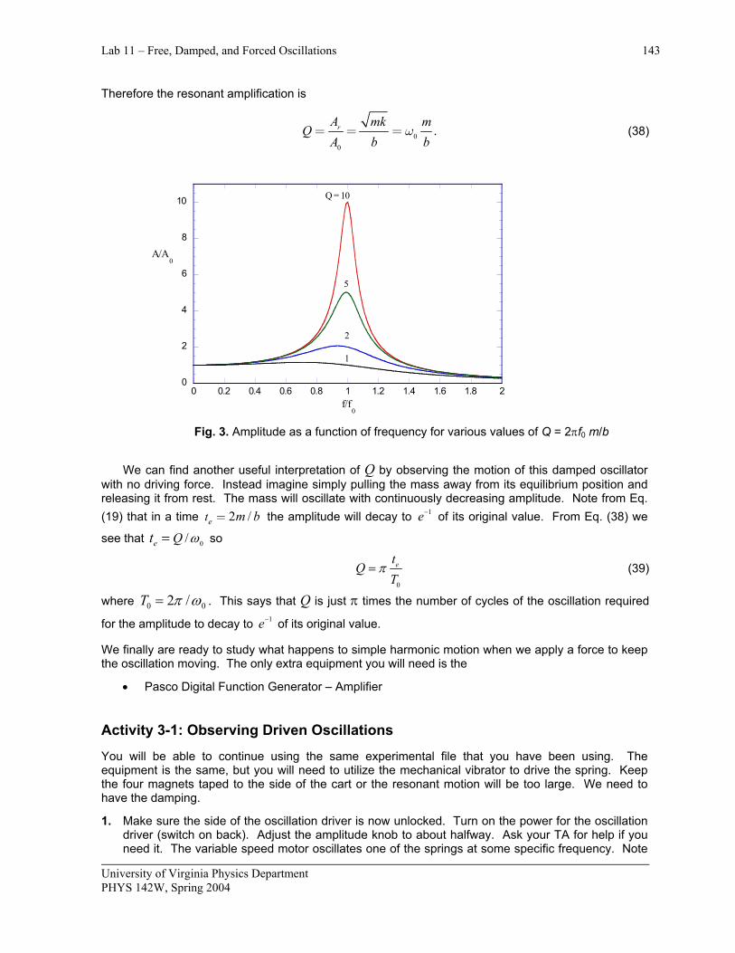
Fig. 3. Amplitude as a function of frequency for various values of Q = 2πf0 m/b We can find another useful interpretation of Q by observing the motion of this damped oscillator with no driving force. Instead imagine simply pulling the mass away from its equilibrium position and releasing it from rest. The mass will oscillate with continuously decreasing amplitude. Note from Eq. (19) that in a time the amplitude will decay to 2 /et m b= 1e− of its original value. From Eq. (38) we

see that 0/e Qt ω= so

0

etQT

π= (39)

where 0 2 /T 0π ω= . This says that Q is just π times the number of cycles of the oscillation required

for the amplitude to decay to e of its original value. 1−

We finally are ready to study what happens to simple harmonic motion when we apply a force to keep the oscillation moving. The only extra equipment you will need is the

• Pasco Digital Function Generator – Amplifier Activity 3-1: Observing Driven Oscillations You will be able to continue using the same experimental file that you have been using. The equipment is the same, but you will need to utilize the mechanical vibrator to drive the spring. Keep the four magnets taped to the side of the cart or the resonant motion will be too large. We need to have the damping.

1. Make sure the side of the oscillation driver is now unlocked. Turn on the power for the oscillation driver (switch on back). Adjust the amplitude knob to about halfway. Ask your TA for help if you need it. The variable speed motor oscillates one of the springs at some specific frequency. Note



that this is frequency f, not angular frequency ω. Set the motor frequency to ~ 0.10 Hz. 2. Make sure the air is on the air track. The vibrator should be moving left and right very slowly. 3. Start the computer and take about 50 s of data and examine the motion. Note visually the phase

relation between the driver and the motion of the cart. Stop the computer and save these data. Question 3-1: Describe the motion of the cart, especially the phase relation between the driver and the motion of the cart. 4. Find the peak-to-peak values of the amplitude distance for the oscillatory motion. We call this 2A

and it refers to the distance between the maximum and minimum values of the oscillation. This can be done easily using the Smart Tool technique of measuring between two points. Ask your TA if you are not familiar with this technique.

2A _____________ (0.1 Hz) 5. You found both angular frequency ω0 and frequency f0 ( f0 = ω0/2π) in step 5 of Activity 1-3. Now

set the driver to a frequency at least twice as high as fo (this should result in a frequency greater than 1.3 Hz). Start the computer again and observe the motion. Note the phase relation between the driver and the motion of the cart. Take about 50 s of data, answer Question 3-2, and stop the computer.

Question 3-2: Describe the motion of the cart, especially the phase relation. 6. Find the peak-to-peak values of the amplitude for this motion. Include the actual frequency that

you used. 2A _______________ (_______ Hz) Prediction 3-1: For what driving frequency fR do you expect to obtain resonant behavior? Write your prediction here. Predicted resonant frequency fR ________________ Hz 7. Now we want to study the motion at the maximum amplitude. One method is by systematically

varying the driving frequency until resonance is found, but that would be quite tedious. Another way is to set the driving frequency to the one you just predicted and try that. You will need to leave the computer running for some time, because it will take several seconds for the system to reach steady-state equilibrium. Try varying the frequency around f0 until you find the maximum motion. You might try the Monitor function while you vary the frequency to determine the maximum motion. What resonant frequency and amplitude did you find?

Experimental resonant frequency fR _______________ Hz Amplitude AR ____________ m



Question 3-3: How well do your two resonant frequencies agree? Would you expect them to be the same? Explain. Activity 3-2: Examination of the Quality Factor Q It is common to describe the degree of damping in an oscillating system by using the Quality Factor Q, which is determined approximately in Eq. (38). This is true when ωR ≈ ω0. Prediction 3-2: Use your experimental values of ω R, m, and b to determine your predicted value of the quality factor. Predicted quality factor ______________ 1. Now we want to be able to produce a graph like that in Fig. 3. You will want to find the amplitude

for some frequencies around the resonant one. You already have data for fR, 0.1 Hz, and 2f. Try frequencies of 0.80fR, 0.90fR, 0.95fR, 1.05fR, 1.10fR, and 1.20fR, around the resonant frequency and find the peak-to-peak amplitude 2A. One group member should continue with the next step 2 while taking these data.

Table 3-1

Frequency f (Hz) Peak-to-peak amplitude, 2A

0.1

0.80 fR =

0.90 fR =

0.95 fR =

fR =

1.05 fR =

1.10 fR =

1.20 fR =

2f =




2. Type your values for all the frequencies f and the amplitudes 2A into Excel and produce a graph

like that shown in Fig. 3 for your data. Just plot 2A versus f instead of A/A0 versus f/f0 that is shown in Fig. 3. Your graph should have the same shape. If you have more time, measure 2A for additional frequencies to fill out the graph you produce. Include your table and graph in your report.

Question 3-4: Does your graph have the shape you expect? Discuss your graph.

lab 11: free damped and forced...

Documents