lab 2 filter implementation 6437 - university of torontodkundur/course_info/real... · to begin,...

http://www.comm.utoronto.ca/~dkundur/course/real-time-digital-signal-processing/

of 1

Lab 2: Filter Design and Implementation Professor Deepa Kundur

Objectives of this Lab This lab

• introduces you to filter design and testing techniques using MATLAB/Simulink;

• gives you a deeper understanding of the filter design techniques automated in MATLAB via the Filter Design & Analysis Tool (FDAT);

• introduces you to hardware implementation of the filtering techniques via MATLAB/Simulink, CCStudio and the Texas Instruments DM6437 DSP board.

Prelab Prior to beginning this lab, you must have carefully read over this lab in order to plan how to

implement the tasks assigned. Make sure you are aware of all the items you need to include in your lab report.

Deliverables • At the beginning of the lab you should submit to your TA the solutions to the prelab

questions.

• During the lab, you must show your TA the Simulink results discussed in the lab instructions; and

• After the lab, each student must submit a separate report answering the questions in this lab.

Grading and Due Date You should have enough time to do the lab in class, but if you do not, please note that you can

come in on your own time to complete the lab requirements. The lab will be graded on correctness, comprehensiveness and the insight you are able to provide when answering the questions. For full points, lab reports should be written in complete sentences with correct grammar.

Please note STRICT DEADLINE for report on the course web site.


of 2

Lab 2: Filter Design and Implementation

Part 1: Filter Design In this lab we will design digital frequency-selective filters to be used to remove or filter out

noise from a signal. Recall the concept of the ideal lowpass filter, which is simply visualized in the frequency domain as the rectangle function (of a specified width and centered at the origin). Also recall that this filter, although handy in theory, is not implemented in practice. There are several reasons why ideal (lowpass, bandpass, highpass, and band-stop) filters are not used in real-life:

1. The impulse response, h(n) is non-causal as a consequence of the Paley-Wiener theorem, which implies these filters cannot be implemented in practice on a DSP. Another way to think about this is that h(n) has infinite support for any of the ideal filters. Thus, it cannot be zero for n < 0 making it necessarily non-causal.

2. When implemented in software or hardware, due to the finite number of elements employed for processing, an ideal filter exhibits the undesirable Gibbs phenomenon. In signal and image processing, this shows up as the infamous ringing effect, i.e. it introduces extra unwanted artifacts.

To bypass the above inadequacies, the design of digital filters using the windowing technique is an alternative to ideal filters. These filters can be implemented as FIR filters, and make use of the well-known Bartlett, Blackman, Hamming, Hanning, and Kaiser windows.

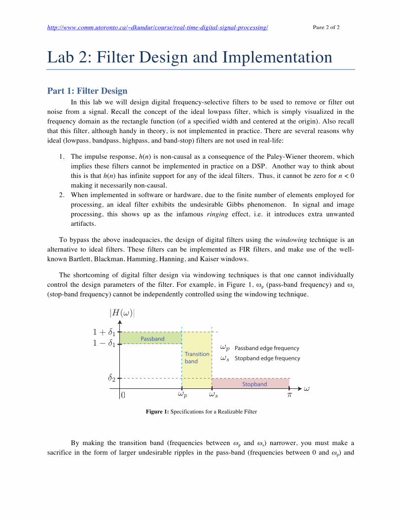
The shortcoming of digital filter design via windowing techniques is that one cannot individually control the design parameters of the filter. For example, in Figure 1, ωp (pass-band frequency) and ωs (stop-band frequency) cannot be independently controlled using the windowing technique.

Figure 1: Specifications for a Realizable Filter

By making the transition band (frequencies between ωp and ωs) narrower, you must make a sacrifice in the form of larger undesirable ripples in the pass-band (frequencies between 0 and ωp) and

Passband ripple

Stopband ripple

Passband edge frequency

Stopband edge frequency

Passband edge frequency

Stopband edge frequency

Passband ripple

Passband

Stopband

Transitionband


of 3

stop-band (frequencies exceeding ωs); that is smaller ωs - ωp necessitates δ1 and δ2 larger These tradeoffs are all due to bypassing the two inadequacies of ideal filters.

The above specifications are general and do not delineate the form of the digital filter. In practice we would prefer either a rational system function corresponding to FIR or IIR filters discussed in the lectures. Thus we consider using the difference equation, or ARMA (autoregressive moving average) model given in (1) and (2) representing the descriptions in the time- and frequency-domain, respectively.

∑ ∑= =

−+−−=N

k

M

kkk knxbknyany

1 0)()()( (1)

∑

∑

=

−

=

−

+= N

k

kk

M

k

kk

za

zbzH

1

0

1)( (2)

Also IIR filters are generally less complex than FIR filters (the difference being that for FIR filters there is a restriction that ak = 0 for all k), as they require fewer parameters and less memory for the same “quality” of filter performance. IIR filters can often be defined analytically as a rational function in the Z-transform domain, and the general description of the filter in Figure 1 is not Z-transform friendly (yet) – it’s analog. Fortunately one can design a filter meeting Figure 1 specifications, and then transform the resulting filter to a Z-transform-friendly filter by using popular transformation techniques such as approximation of derivatives, impulse response, bilinear transformation (most popular), and matched Z-transform techniques. Luckily, MATLAB has a nice little GUI driven filter design program, which requires we to do no more than click a few buttons …

Design and Implementation

Filter Design and Analysis Tool In this section, you will learn how to use MATLAB’s handy Filter Design & Analysis Tool

(FDAT). To begin, start MATLAB. Now, enter fdatool into the command window. This should, when executed, bring up the FDAT’s graphical user interface (GUI), shown in Figure 2 below.

The process of designing a filter is fairly self-explanatory: you simply set all of the filter specifications in the lower half of the GUI. When you are satisfied with your specifications, click on the Design Filter button. The magnitude response of the resulting filter will appear in the Magnitude Response pane. Note that you can view the coefficients of the filter’s transfer function in second order sections by clicking on the Filter coefficients button at the top of the GUI (which looks like [b,a]).


of 4

Figure 2: Filter Design and Analysis Tool

One useful feature of FDAT is that you can store multiple filters at once and switch between them as you wish. After you have designed a filter, you can store it by selecting the Store Filter button; this will prompt you to enter a name for the filter. Once you have stored the filter, you can begin designing a new filter by choosing new filter specifications. To access previously stored filters, click on the Filter Manager button. Finally, you can save all of your stored filters in one “session” by selecting File → Save Session As; this will save your session with a .fda extension. You can always open previously saved sessions in the FDAT GUI.

Another cool feature of FDAT that we will be using is to export filters to a Simulink model as a single-input, single-output block. To do this, make sure the filter you want is currently shown in the GUI (if not, switch to it using the Filter Manager). Then, click on File → Export to Simulink Model; a new set of options should appear in the lower half of the GUI. Give the filter a good, descriptive Block Name and make sure the Destination is Current. Press the Realize Model Button (this only works if you have a Simulink Model currently open, of course).

Designing the Filters Before implementing anything, a good engineer always makes sure not to bypass the design stage. In FDAT, perform the following tasks, assuming a sampling rate of 8 kHz:

1. Design a minimum order, stable1, lowpass Butterworth filter with a passband frequency of 1 kHz and a stopband frequency of 1.4 kHz. Make the attenuation 1 dB at the passband frequency and 80 dB at the stopband frequency.

2. Design a minimum order, stable, lowpass Chebyshev Type I filter with the same specifications as the Butterworth filter.

1 You can verify that a filter is stable after you have designed it by clicking on the Filter information button ( )


of 5

3. Design a lowpass FIR filter using the Blackman Window with a cutoff frequency of 1 kHz. Specify the order of the filter such that the first minimum in the stopband (preceding the first lobe) is as close to 1.4 kHz as possible without exceeding it.

Lab Report Questions 1. What is the order of the lowpass Butterworth filter you designed? 2. What is the order of the lowpass Chebyshev Type I filter you designed? 3. Compare the memory usage of each of the 3 filters assuming a Direct Form II realization is

employed. Do you see how inefficient the windowing technique is? How much more expensive in terms of memory is the windowing technique from the best IIR filter?

Designing the Filters in Simulink This is where you make it or break it. You’ve glued the wings on your Ford F-150, and now it’s

time to see if it will fly. To test the filters, you will input a sine wave that has been corrupted by noise, like in Lab 1. First, you will test each of the filters in non-real time. Then you will implement them using the DM6437 DSP board.

Simulation In this section, you’ll simulate each one of the filters you designed for a finite duration in non-

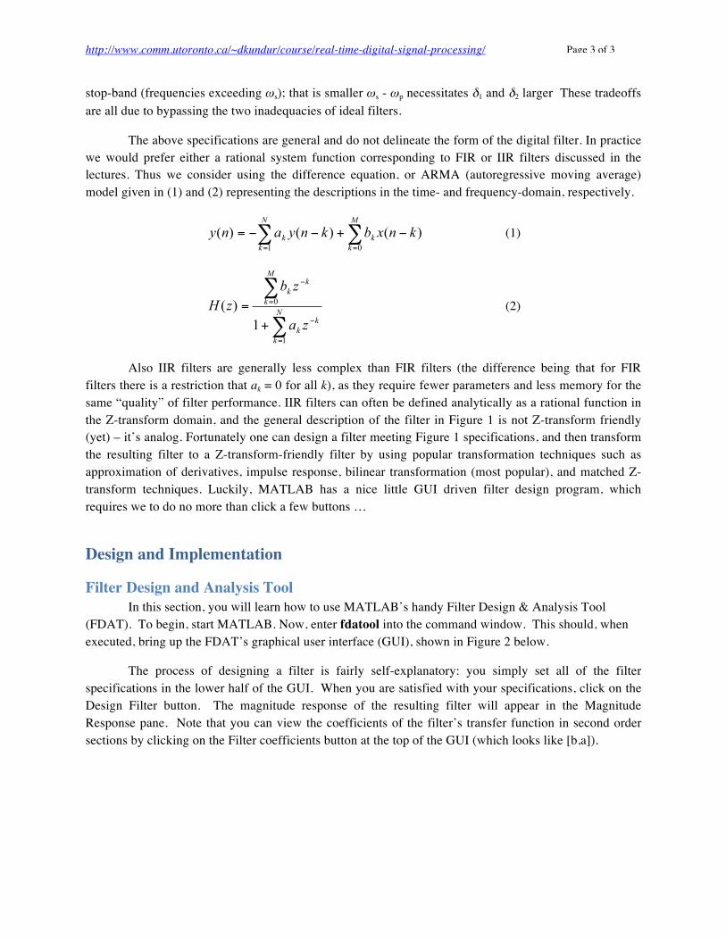
real-time. Open a new Simulink model and construct a block diagram similar to that shown in Figure 3 below. Before your begin, please note the following about the block diagram:

1. The Digital Filter block labeled “Filter” is the result of exporting a filter from FDAT to Simulink; this is where you’ll place the filters you designed.

2. The input to the filter is a noisy sinusoid. The high frequency noise is created in the same way as in Lab 1. That is, the random number generator must generate numbers between -5 and 5. The highpass filter block should have an impulse response that is IIR, a minimum order, frequency in units of Hz, a Fs of 8000, Fstop of 3600, Fpass of 3800, Astop of 60 and Apass of 1. It may make things easier to bring a hardcopy of the Lab 1 instructions to this lab. Please also note that the highpass filter will have to be appropriately replaced to generate different types of noise in this lab.

3. The Sine Wave source block is a continuous-time source. The Zero-Order Hold block is used to convert it to discrete-time and thus acts like an analog-to-digital converter. Make sure that the zero-order hold is set to the same sampling rate that your filters were designed for.

4. The Smoothing Filter is just a lowpass analog filter that interpolates the digital output of the Digital Filter and thus acts like a digital-to-analog converter. You can obtain the Analog Filter Design block. Recall from DSP theory that the cutoff frequency of this filter should be half of the sampling frequency. Also, note that you can choose whatever type of analog filter you wish (i.e. it doesn’t have to be a Chebyshev Type II filter, as shown in the Figure). Finally, you’ll want to choose a reasonably low filter order (like 4) because an analog filter tends to be the computational bottleneck that impedes the real-time simulation greatly.

5. For any scope output, to ensure that a greater number of points are stored and hence displayed, on the scope window go to Parameters → Data History. Enter an appropriate number for the “Limit data points to last” field.


of 6

Figure 3: Filter Testing in Simulink.

In Simulink, go to Simulation → Configuration Parameters. Please keep in mind to be sure that the solver type is variable-step. Also, choose ode45 for the solver.

Test each of the three filters you designed in the block diagram of Figure 3 (to change filters, just delete the old one and import a different one from FDAT). Specifically, perform the following tasks for each filter, noting the various filter responses in your report. For every case, save and insert the oscilloscope displays on your report. Please provide information on the specific frequencies used for the sinusoidal source and the filter parameters used for generating the noise. Write down any observation that you may have about the signals and interpret the obtained results.

1. Generate and test sine waves with frequencies in the following regions. For each frequency, set the stop time of the simulation so that you can see several periods of the sine wave. For these tests, you can disconnect the noise from the input signal and terminate it with a Terminator block.

a. Passband region b. Transition region c. Stopband region

2. Reconnect the noise to the input signal. Change the frequency of the sine wave to be in the passband and set the stop time of the simulation appropriately. Add noise to the sine wave whose frequency is in the following three regions (Note: in order to contain the noise to the correct region, you’ll have to change the filter after the noise generator to the appropriate highpass, lowpass, or bandpass filter):

a. Passband region b. Transition region c. Stopband region

3. To measure the effectiveness of your noise filtering approach, using basic Simulink blocks, find a way to calculate the mean squared error between the input sine wave (without noise) and the output of the overall system (please note that if your filter shifts the sine wave so it has a different shift/phase compared to the original source, then you must reshift it back before you compute this error so that both the original and filtered sinusoids are aligned). Please show how you implement this in your report; you may need a different shift for


of 7

each of your filters. Discuss the performance of each filter for the various input sinusoid and noise considered. Explain in what situations you have the best/worst mean square error and why.

Therefore, to test each of your filters, please make sure that the sine wave is set to a frequency in the passband. Then, add noise to the sine wave whose frequency is in the following three regions: passband, transition and stopband. Run a simulation for each type of noise. Repeat this for all three filters you designed. For every case, save and insert the oscilloscope displays on your report. Write down any observation that you may have about the signals and interpret the your results.

Part 2: Hardware Implementation In this lab, you will take your filter designs from Part 1 and implement and test them on the

C6437 DSP board. You will use Simulink’s add-on blockset called Target for TI C6000, which provides blocks to interface the C6437 to a Simulink model. Namely, this blockset contains a source block called ADC, which represents the board’s analog-to-digital converter, as well as a sink block called DAC, which represents the board’s digital-to-analog converter. These blocks will essentially replace the input and output of your other Simulink models. You can find both of them in the Simulink Library Browser under Target for TI C6000 → C6437 DSK Board Support. Additionally, the Target for TI C6000 has a block called C6437DSK under Target for TI C6000 → C6000 Target Preferences. This block has no inputs or outputs; it just kind of floats in the middle of the block diagram. It must be placed in any Simulink model that is to be implemented on the C6437 board; it tells Simulink what type of target it is dealing with. Finally, the blockset includes a block called Switch under Target for TI C6000 → C6437 DSK board support; it allows you to program the three manual switches available on the board.

Figure 1 shows a picture of the C6437 board (from the Texas Instruments DaVinci processor series) with user interfaces with the principal components which the TA will highlight in the lab. In the labs in this course, you will use the input and the output ports (including for audio and video) as well as the manual switches, power plug, USB connector to the PC and Ethernet port.

Figure 1. C6437 Overview. Picture courtesy of Christopher Byers.


of 8

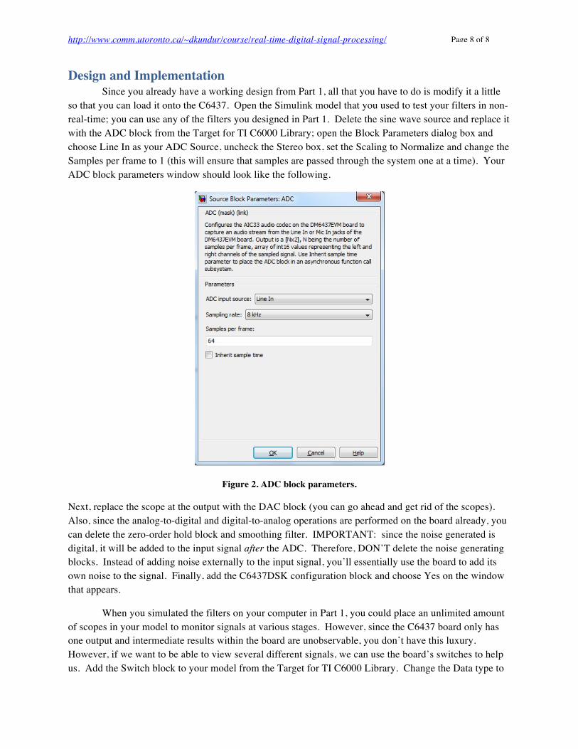
Design and Implementation Since you already have a working design from Part 1, all that you have to do is modify it a little so that you can load it onto the C6437. Open the Simulink model that you used to test your filters in non-real-time; you can use any of the filters you designed in Part 1. Delete the sine wave source and replace it with the ADC block from the Target for TI C6000 Library; open the Block Parameters dialog box and choose Line In as your ADC Source, uncheck the Stereo box, set the Scaling to Normalize and change the Samples per frame to 1 (this will ensure that samples are passed through the system one at a time). Your ADC block parameters window should look like the following.

Figure 2. ADC block parameters.

Next, replace the scope at the output with the DAC block (you can go ahead and get rid of the scopes). Also, since the analog-to-digital and digital-to-analog operations are performed on the board already, you can delete the zero-order hold block and smoothing filter. IMPORTANT: since the noise generated is digital, it will be added to the input signal after the ADC. Therefore, DON’T delete the noise generating blocks. Instead of adding noise externally to the input signal, you’ll essentially use the board to add its own noise to the signal. Finally, add the C6437DSK configuration block and choose Yes on the window that appears.

When you simulated the filters on your computer in Part 1, you could place an unlimited amount of scopes in your model to monitor signals at various stages. However, since the C6437 board only has one output and intermediate results within the board are unobservable, you don’t have this luxury. However, if we want to be able to view several different signals, we can use the board’s switches to help us. Add the Switch block to your model from the Target for TI C6000 Library. Change the Data type to


of 9

Integer and the Sample time to 1/8000. As you can see, the Switch block acts like a source in your model; it outputs an integer that corresponds to the current setting of the three manual switches. To see which switch settings correspond to which integer outputs, right-click on the Switch block and select Help.

Now, add two Multiport Switches from Simulink → Signal Routing in the following overall configuration:

Figure 3. Switch configuration.

Your model is now ready to load onto the board and run. You will now use Real-Time Workshop to build C-code from your model that is portable to the C6437 board. Also, you’ll use MATLAB’s Link for Code Composer Studio to export this code to Code Composer Studio 3.3. Follow these instructions:

1. Simulation→ Configuration Parameters a. Go to Hardware Implementation under the Select tree and change the Device type to TI

C6000 b. Go to Solver under Select tree

i. Stop time: inf ii. Fixed-step

iii. Discrete solver iv. Fixed-step size (fundamental sample time): 1/8000 v. Tasking mode for periodic sample times: Single Tasking

c. Go to Real-Time Workshop under Select tree i. Under Target selection, click Browse

ii. Select ccslink_grt.tlc from the list and press OK d. Go to Link for CCS

i. Under Project Options, select Custom; in the Compiler options string, type –o2 –q ; set the System stack size to 8192.

ii. Under Runtime, set the Build action to Build and Execute. e. Press OK

2. In Simulink, choose Tools→ Real-Time Workshop→ Build Model (after a few moments of processing, the command window will say if build is successful or not).


of 10

3. If MATLAB reports that the build is successful, CC Studio will have compiled the code that was just created in MATLAB. In CC Studio, you should see that the build was successful. Also, you should see that a new project was created; if you wish, you can look through this project to see all of the source code that was created from your model (don’t change any of it, of course!). If the build is not successful, sometimes restarting MATLAB and Simulink might do the trick. However if the build is still not successful after this, notify your TA of the error.

4. At this point the program you just built should have been loaded automatically on the board and it should also be running. If this is the case, you can skip the next 3 steps, otherwise don’t skip them or your program will not run.

5. In CC Studio, reset your board’s processor by selecting Debug → Reset 6. Select File → Load Program to load the code onto your board. 7. If the load was successful, you can run the program. To do this, select Debug → Run.

At any time, you can stop your program from running by choosing Debug → Halt. If you run into problems, you can always try to reset your board and load the program again. However, if you choose to reset the board, you must also restart all of MATLAB, Simulink and CCStudio to avoid memory errors. If this isn’t enough, you may have to disconnect from your board (Debug → Disconnect), reset the emulator (Debug → Reset Emulator), and reconnect to your board.

The next step after you get the program to run is to test its functionality. This should be fairly straight forward IF you have a properly working model compiled on the board. Connect the output jack on the board to the oscilloscope. Then connect the function generator output to the input jack on the board. Next, set the waveform to a sinusoid with magnitude (peak-to-peak) of 2 volts. Perform the following tasks. For every case, draw or copy the oscilloscope displays on your report. Write down any observation that you may have about the signals and interpret the obtained results:

1. Test the following frequencies: 100, 1000, 3800, and 5000 Hz. For each of the frequencies, use the board’s switches to compare the input and output waveforms; note any differences and explains why this might occur. It is best to keep the scale on the oscilloscopes the same (i.e., do not auto-scale) and note the differences.

2. Show that the filter works by using the DSP board switches to alternate between the noisy input, the noise, the input, and the output. Connect the output to speakers and show your results to the Teaching Assistant for a 100 Hz Sinusoidal.

3. Now, for comparison, try a Square wave and a Triangle at 100, 3800, and 5000 Hz. Compare the input and output waveforms visually and note any differences and explain why this might occur.

lab 2 filter implementation 6437 - university of torontodkundur/course_info/real... · to begin,...

Documents