1

NORTHERN ILLINOIS UNIVERSITY PHYSICS DEPARTMENT

Physics 253 – Fundamental Physics Mechanic, September 23, 2010

Lab #4 An Introduction to Error Analysis

Lab Write-up Due: Thurs., September 30, 2010 Place of meeting TBD

Read Giancoli: Chapter 3

I. Introduction Physics is an experimental science. The physicist uses mathematics but the models he or she constructs aren’t abstract fantasies—they describe the real world. All physical theories are inspired by experimental observations of nature and must ultimately agree with these observations to survive. The interplay between theory and experiment is the essence of modern science. The task of constructing a theory, inherently difficult, is compounded by the fact that observations are never perfect. Because instruments and experimenters depart from the ideal, measurements are always slightly uncertain. This uncertainty appears as variations between successive measurements of the same quantity. With better instrumentation and greater care, these fluctuations can be reduced but they can never be completely eliminated*. One can, however, estimate how large the uncertainty is likely to be and to what extent one can trust the measurements. Over the years powerful statistical methods have been devised to do this. In other words, the experimenter can rigorously describe the limitation of his or her measurements. In an imperfect world we can expect no more; and once we understand the limitations of an experiment we can, if we feel the need, try to improve on it. In the laboratory you, like any scientist, will have to decide just how far you can trust your observations. Here is a brief description of experimental uncertainties and their analysis. Your TA will indicate how far you need to carry the analysis in each experiment. Today we’ll give you the background to analyze the projectile motion laboratory with proper error analysis.

* In certain instances, there is a fundamental limit imposed on this process of improvement. Quantum mechanics, which deals with very small systems such as atoms and nuclei, suggests that there is an inherent uncertainty in nature that even perfect instrumentation cannot overcome. Luckily, most experiments do not confront this ultimate barrier.

2

II. Definitions

The difference between the observed value of a quantity and the true value is called the error of the measurement. This term is misleading; it does not necessarily imply that the experimenter has made a mistake. If this was the case the experimenter would naturally correct it! “Uncertainty” is a better term but it is not as commonly used, and we’ll use them interchangeably here. Errors or uncertainties may be conveniently classified into three types: A. Illegitimate Errors: These are the true mistakes or blunders either in measurement

or in computation. Reading the wrong scale or misplacing a decimal point are examples. These errors usually stand out if the data is examined critically. You can correct such errors when you find them by eliminating their cause and possibly by repeating the measurement. If it’s too late for that, you can at least guess where the mistake is likely to lie.

B. Systematic Errors: These errors arise from faulty calibration of equipment, biased

observers, or other undetected disturbances that cause the measured values to deviate from the true value—always in the same direction. The bathroom scale that read –3 lbs before anyone steps on it exhibits a systematic error. These errors cannot be adequately treated by statistical methods. They must be estimated and, if possible, corrected from an understanding of the experimental techniques used. Systematic errors affect the accuracy of the experiment; that is, how closely the measurements agree with the true value.

C. Random Errors: These are the unpredictable fluctuations about the average or

“true” value that cannot be reduced except by redesign of the experiment. These errors must be tolerated although we can estimate their size. Random errors affect the precision of an experiment; that is, how closely the results of successive measurements are grouped.

An experiment may be accurate but not precise—or precise but not accurate. To remember the distinction let’s imagine a game of darts: A thrower is accurate if all of her shots hit the bull’s-eye, if they hit anywhere else and she’s not. However if all of her shots are tightly grouped she’s precise no matter where they are centered. The concepts of error analysis that are introduced below are strictly applicable only to random errors.

III. Practices and Concepts The result of a measurement is usually recorded as

!

A ± "A where A is the best guess for the value and

!

"A means “the change in A”. The interpretation is that the true value of A lies between

!

A "#A and

!

A + "A . The length of a wood block recorded as 15 2 0 3.. ± cm would be expected to lie between 14.9 and 15.5 cm.

3

A. Significant Figures: The number of figures in a result A is, by itself, often indicative

of the uncertainty. In the example above, the value of 15.2 cm implies that the error will be at most several tenths of a cm since it isn’t physically realistic to compute an error to more than one (occasionally two) significant figures. Accordingly, it wouldn’t make sense to write the result as 15 0 3.± cm since writing 15 implies that we know nothing about tenths of centimeters. Likewise, writing 15 2 1. ± cm is inconsistent. The result and the error estimate must always be in agreement concerning the least uncertain decimal place.

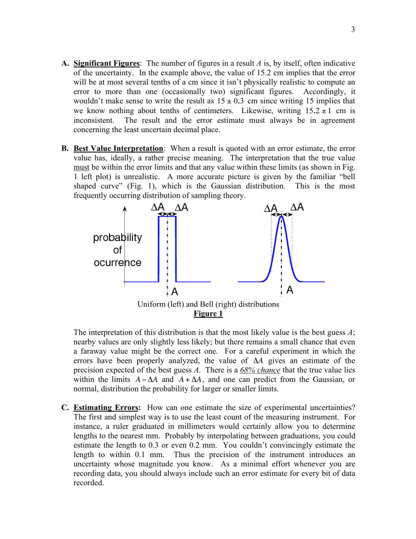
B. Best Value Interpretation: When a result is quoted with an error estimate, the error

value has, ideally, a rather precise meaning. The interpretation that the true value must be within the error limits and that any value within these limits (as shown in Fig. 1 left plot) is unrealistic. A more accurate picture is given by the familiar “bell shaped curve” (Fig. 1), which is the Gaussian distribution. This is the most frequently occurring distribution of sampling theory.

Uniform (left) and Bell (right) distributions

Figure 1

The interpretation of this distribution is that the most likely value is the best guess A; nearby values are only slightly less likely; but there remains a small chance that even a faraway value might be the correct one. For a careful experiment in which the errors have been properly analyzed, the value of

!

"A gives an estimate of the precision expected of the best guess A. There is a 68% chance that the true value lies within the limits

!

A "#A and

!

A + "A , and one can predict from the Gaussian, or normal, distribution the probability for larger or smaller limits.

C. Estimating Errors: How can one estimate the size of experimental uncertainties?

The first and simplest way is to use the least count of the measuring instrument. For instance, a ruler graduated in millimeters would certainly allow you to determine lengths to the nearest mm. Probably by interpolating between graduations, you could estimate the length to 0.3 or even 0.2 mm. You couldn’t convincingly estimate the length to within 0.1 mm. Thus the precision of the instrument introduces an uncertainty whose magnitude you know. As a minimal effort whenever you are recording data, you should always include such an error estimate for every bit of data recorded.

4

D. Repeated Measurements: When there is time or when the piece of data is crucial,

you can repeat the measurement several times. The scattering of values about the average provides an estimate of the magnitude of the random error. For instance, in the set of measurements 1.0, 1.1, 1.3, 0.9, 1.3 cm, a reasonable guess for the best value is the average, 1.1 cm, and the uncertainty in each measurement seems to be about 0.2 cm.

1. Best Value: Statistical analysis shows, not surprisingly, that the average, or

mean, of a set of measurements provides the best estimate of the true value. This is simply the sum of the measurements divided by the number of measurements taken:

!

x "1

Nx

i

i=1

N

#

where

!

x is the mean of the N measurements of the quantity x , labeled i

x where the index i runs from 1 to N.

2. Standard Deviation: The best estimate of the uncertainty of a measurement is

shown by statistics to be the standard deviation. The sample standard deviation is found by taking the differences of each

ix value from the mean, squaring these

differences and added them, dividing by N-1, and then taking the square root:

!

"s#

1

N $1x

i$ x ( )

2

i=1

N

%

The factor (N-1) implies that for N=1, 0 0/S

! = : the standard deviation is indeterminate. In other words: from only one measurement it is impossible to say anything about the random experimental uncertainty.

3. Standard Error of the Mean: The standard deviation is not quite the error

estimate that is needed. The sample standard deviation, S

! , is the estimated uncertainty of each individual measurement

ix . The value

S! fluctuates as more

samples are taken, but it doesn’t systematically get smaller. Haven taken N repeated measurements, our estimate of the true value is the mean, x . The standard error (or standard deviation) of the mean is the estimate of the error in this value. The standard error of the mean is related to the standard deviation of a measurement by a simple expression:

!

"m

="s

N

The derivation of this result is more appropriate for a statistics class, for our purposes we’ll accept the result as true. Note that the uncertainty of the mean is reduced by a factor of

!

N from the uncertainty in an individual measurement. This is the reason for repeatedly measuring the same quantity. Note, however,

5

that the reduction is only by

!

N . Making 100 measurements instead of 10 only reduces the uncertainty by a factor of 3! Calculating the standard deviation can be tedious. However there are programs for computers and programmable calculators which give the mean and standard deviation of a series of entries. Some scientific calculators have this program built in.

Example: Suppose we measured the length of a line four times and obtained values of 5.5, 5.3, 4.9, 4.7 cm. These values sum to 20.4 cm, and our best

estimate of the length is the mean value ( )120 4 5 1

4..x = = cm. The error

estimate associated with each measurement is the standard deviation:

( ) ( ) ( ) ( )2 2 2 21

5 5 5 1 5 3 5 1 4 9 5 1 4 7 5 1 0 373

.........S

! " #= $ + $ + $ + $ =% & cm

The set of four measurements taken together gives us an estimated error m

! of the mean:

0 370 18

4

..

m! = = cm

The final result then for the length of the line is: 5 1 0 2.. ± cm.

IV. Significant Figures There is a natural shorthand for indicating uncertainties called significant figures. The measurement 15.23 cm, for example, has four significant figures; it is uncertain to a few one-hundredths of a centimeter (the exact uncertainty is deliberately left vague). It is different from 15 cm, 15.2 cm, 15.230 cm, and 15.2300 cm; those numbers might all represent the same measurement, but the uncertainty is different in each case by an order of magnitude. It makes no difference, however, whether we write 15.23 cm, 0.l523 m, or 152.3 mm; each number has four significant figures. A number with m significant figures has a fractional uncertainty of 1 part in 10m . In adding or subtracting numbers, the largest uncertainty will dominate. This belongs to the number whose least significant figure is farthest to the left (that is, the last significant digit of the most imprecise number); the sum (or differences) will have no significant figures beyond this point. For instance, adding the numbers below gives:

15 2304

2 13

489 5

62

956

.

.

.

6

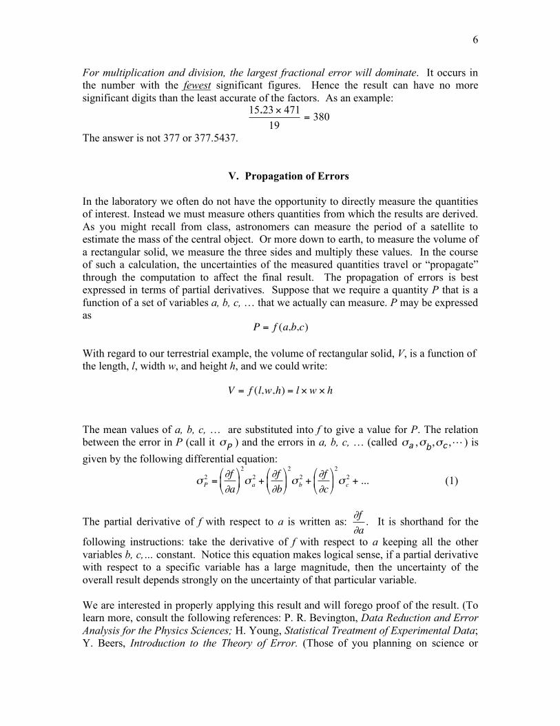
For multiplication and division, the largest fractional error will dominate. It occurs in the number with the fewest significant figures. Hence the result can have no more significant digits than the least accurate of the factors. As an example:

15 23 471380

19

. !=

The answer is not 377 or 377.5437.

V. Propagation of Errors

In the laboratory we often do not have the opportunity to directly measure the quantities of interest. Instead we must measure others quantities from which the results are derived. As you might recall from class, astronomers can measure the period of a satellite to estimate the mass of the central object. Or more down to earth, to measure the volume of a rectangular solid, we measure the three sides and multiply these values. In the course of such a calculation, the uncertainties of the measured quantities travel or “propagate” through the computation to affect the final result. The propagation of errors is best expressed in terms of partial derivatives. Suppose that we require a quantity P that is a function of a set of variables a, b, c, … that we actually can measure. P may be expressed as

!

P = f (a,b,c) With regard to our terrestrial example, the volume of rectangular solid, V, is a function of the length, l, width w, and height h, and we could write:

!

V = f (l,w,h) = l " w " h

The mean values of a, b, c, … are substituted into f to give a value for P. The relation between the error in P (call it

P! ) and the errors in a, b, c, … (called a! ,

b! , c! ,L ) is

given by the following differential equation:

!

"P

2=#f

#a

$

% &

'

( )

2

" a

2+#f

#b

$

% &

'

( )

2

" b

2+#f

#c

$

% &

'

( )

2

" c

2+ ... (1)

The partial derivative of f with respect to a is written as:

!

"f

"a. It is shorthand for the

following instructions: take the derivative of f with respect to a keeping all the other variables b, c,… constant. Notice this equation makes logical sense, if a partial derivative with respect to a specific variable has a large magnitude, then the uncertainty of the overall result depends strongly on the uncertainty of that particular variable. We are interested in properly applying this result and will forego proof of the result. (To learn more, consult the following references: P. R. Bevington, Data Reduction and Error Analysis for the Physics Sciences; H. Young, Statistical Treatment of Experimental Data; Y. Beers, Introduction to the Theory of Error. (Those of you planning on science or

7

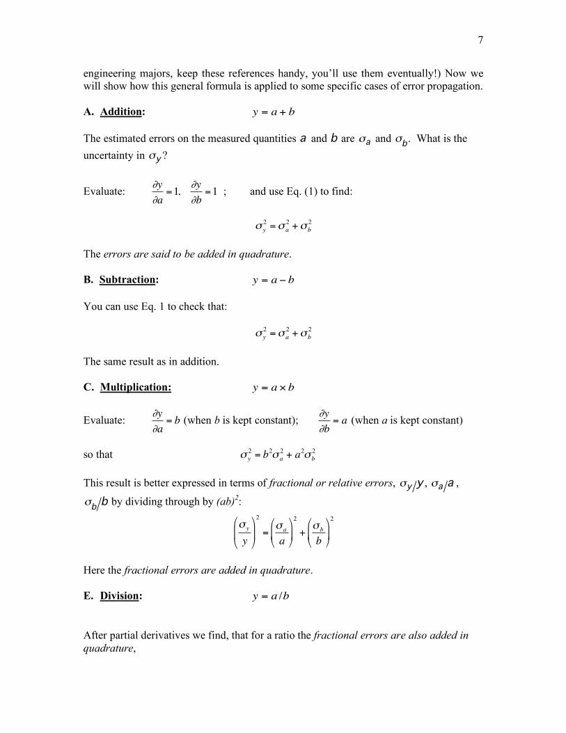
engineering majors, keep these references handy, you’ll use them eventually!) Now we will show how this general formula is applied to some specific cases of error propagation. A. Addition:

!

y = a + b The estimated errors on the measured quantities a and b are a! and

b! . What is the

uncertainty in y! ?

Evaluate:

!

"y

"a=1,

"y

"b=1 ; and use Eq. (1) to find:

!

" y

2=" a

2+" b

2 The errors are said to be added in quadrature. B. Subtraction:

!

y = a " b You can use Eq. 1 to check that:

!

" y

2=" a

2+" b

2 The same result as in addition. C. Multiplication:

!

y = a " b

Evaluate:

!

"y

"a= b (when b is kept constant);

!

"y

"b= a (when a is kept constant)

so that

!

" y

2= b

2" a

2+ a

2" b

2 This result is better expressed in terms of fractional or relative errors, y y! , a a! ,

bb! by dividing through by (ab)2:

!

" y

y

#

$ %

&

' (

2

=" a

a

#

$ %

&

' (

2

+" b

b

#

$ %

&

' (

2

Here the fractional errors are added in quadrature. E. Division:

!

y = a /b After partial derivatives we find, that for a ratio the fractional errors are also added in quadrature,

8

!

" y

y

#

$ %

&

' (

2

=" a

a

#

$ %

&

' (

2

+" b

b

#

$ %

&

' (

2

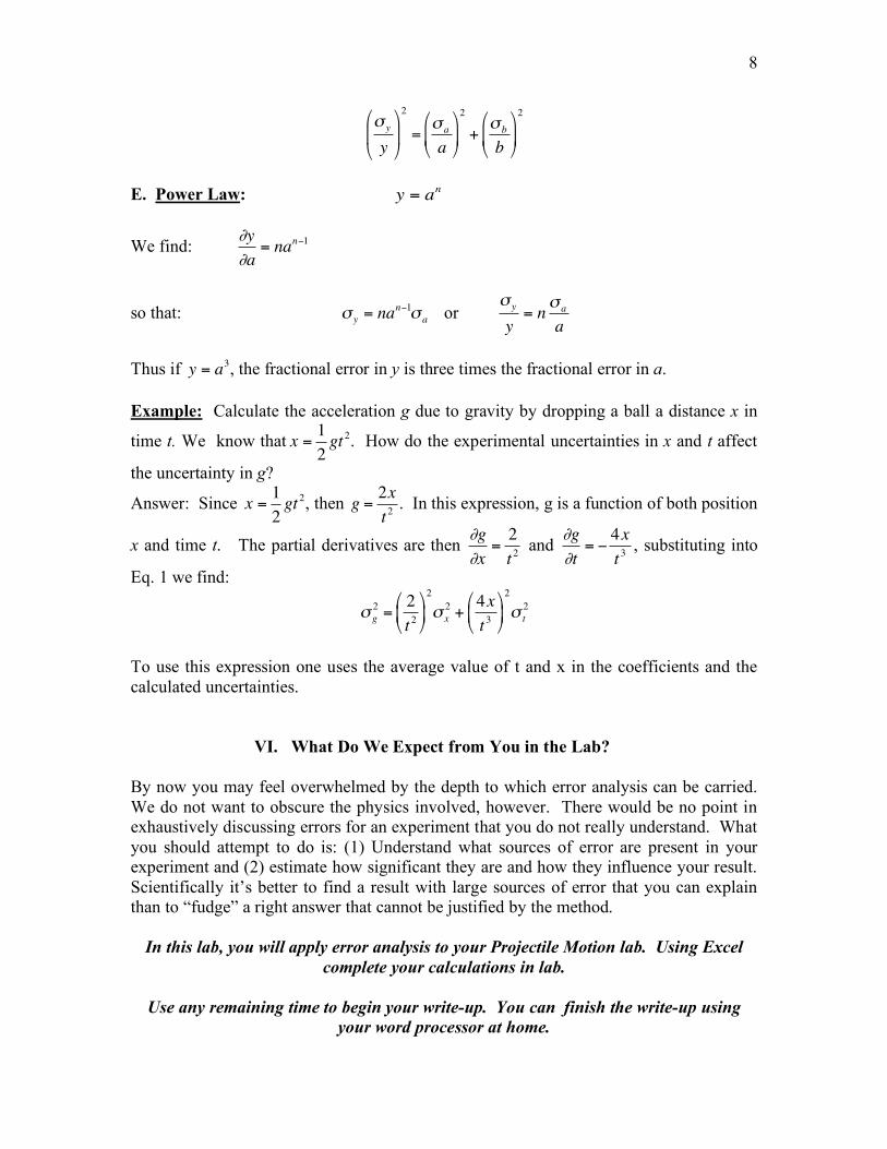
E. Power Law:

!

y = an

We find:

!

"y

"a= na

n#1

so that:

!

" y = nan#1" a or

!

" y

y= n

" a

a

Thus if

!

y = a3, the fractional error in y is three times the fractional error in a.

Example: Calculate the acceleration g due to gravity by dropping a ball a distance x in

time t. We know that

!

x =1

2gt

2. How do the experimental uncertainties in x and t affect

the uncertainty in g?

Answer: Since

!

x =1

2gt

2, then

!

g =2x

t2

. In this expression, g is a function of both position

x and time t. The partial derivatives are then

!

"g

"x=2

t2

and

!

"g

"t= #

4x

t3

, substituting into

Eq. 1 we find:

!

" g

2=2

t2

#

$ %

&

' (

2

" x

2+4x

t3

#

$ %

&

' (

2

" t

2

To use this expression one uses the average value of t and x in the coefficients and the calculated uncertainties.

VI. What Do We Expect from You in the Lab? By now you may feel overwhelmed by the depth to which error analysis can be carried. We do not want to obscure the physics involved, however. There would be no point in exhaustively discussing errors for an experiment that you do not really understand. What you should attempt to do is: (1) Understand what sources of error are present in your experiment and (2) estimate how significant they are and how they influence your result. Scientifically it’s better to find a result with large sources of error that you can explain than to “fudge” a right answer that cannot be justified by the method.

In this lab, you will apply error analysis to your Projectile Motion lab. Using Excel complete your calculations in lab.

Use any remaining time to begin your write-up. You can finish the write-up using

your word processor at home.

9

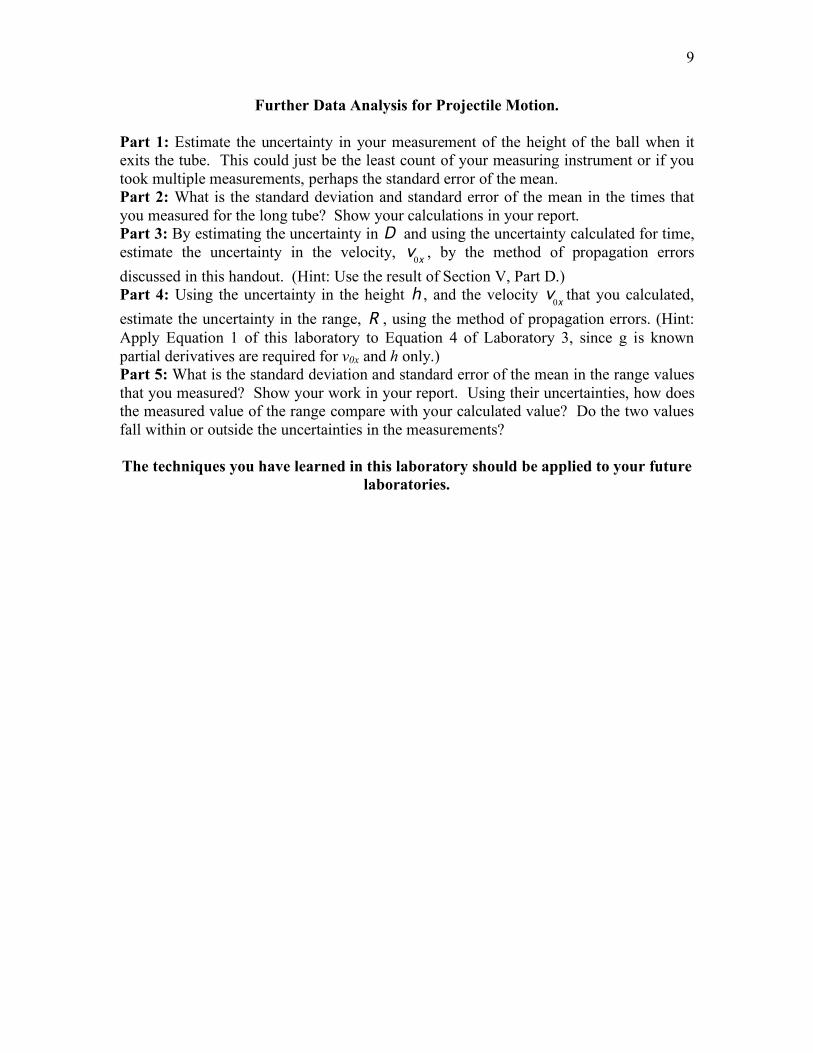
Further Data Analysis for Projectile Motion. Part 1: Estimate the uncertainty in your measurement of the height of the ball when it exits the tube. This could just be the least count of your measuring instrument or if you took multiple measurements, perhaps the standard error of the mean. Part 2: What is the standard deviation and standard error of the mean in the times that you measured for the long tube? Show your calculations in your report. Part 3: By estimating the uncertainty in D and using the uncertainty calculated for time, estimate the uncertainty in the velocity,

0xv , by the method of propagation errors

discussed in this handout. (Hint: Use the result of Section V, Part D.) Part 4: Using the uncertainty in the height h , and the velocity

0xv that you calculated,

estimate the uncertainty in the range, R , using the method of propagation errors. (Hint: Apply Equation 1 of this laboratory to Equation 4 of Laboratory 3, since g is known partial derivatives are required for v0x and h only.) Part 5: What is the standard deviation and standard error of the mean in the range values that you measured? Show your work in your report. Using their uncertainties, how does the measured value of the range compare with your calculated value? Do the two values fall within or outside the uncertainties in the measurements? The techniques you have learned in this laboratory should be applied to your future

laboratories.