Lab 5: Harmonic Oscillations and Damping

I. IntroductionA. In this lab, you will explore the oscillations of a mass-spring system, with and without damping. You'll get to see how changing

various parameters like the spring constant, the mass, or the amplitude affects the oscillation of the system. You'll also see what the effects of damping are, and explore the three regimes of underdamped, critically damped, and overdamped systems. Finally, you will see the effects of a driving force on a harmonic oscillator.

There is no error analysis in this lab. Try to think about the different physics effects and understand the concepts.The final part is the most fun. The groups will be split in two sets. Each will explore a slightly different system. You should talk with your colleagues at the end to find out about their results.

II. Lab goalsA. Learn how to numerically and graphically characterize oscillatory motionB. See how springs work in combination, both in series and in parallelC. See how the oscillation frequency depends on k and mD. Add damping to a harmonic oscillator system and observe its change in behaviorE. Vary the amount of damping to see the three different damping regimesF. See the effect of a driving force in a harmonic oscillator

III. Prelab Assignment

A. This lab covers lectures 19 and 20. Read through the lecture notes. You should also read chapter 13 of Young & Freedman, in particular the sections on damped harmonic motion and forced (or driven) oscillations (sections 13.7 and 13.8).

B. Read this handout.C. Answer the following questions and turn them in at the start of lab. Be sure to put your name, your lab TF's name, and your lab

section at the top of your paper. 1. Suppose two springs, with spring constants k1 and k2, are connected in parallel to a mass as shown.

Assume the springs have the same equilibrium length. If the mass is displaced (vertically) from equilibrium, it will begin to oscillate harmonically.a. What is the effective spring constant of the two combined springs? In other words, if the total spring force on the mass is still

proportional to its displacement from equilibrium, what is the proportionality constant?

b. What is the angular frequency of the oscillation?

2. Same questions, except for the series combination of springs shown below:

2-1

2

Hint: it's the same as before, except this time you'll have to figure out how much each spring stretches as the mass moves. Can Newton's 3rd Law help you?

3. Complete the following table for each value of the damping constant.

Damping Motion General equation of motion Approximate equation of How fast it trends toConstant (γ) type x(t)= motion for large t x = 0

γ = 0 never

γ < ω0

γ = ω0

γ > ω0

IV. Background

A. Harmonic motionMost of what you need to know about harmonic motion has been covered in the lectures and Young & Freedman chapter 13, so we won't repeat it in depth here. The basic idea is that simple harmonic motion follows an equation for sinusoidal oscillations:

For a mass-spring system, the angular frequency, ω0, is given by

where m is the mass and k is the spring constant. Note that ω0 does not depend on the amplitude of the harmonic motion.B. Damping

1. The situation changes when we add damping. Damping is the presence of a drag force or friction force which is non-conservative; it gradually removes mechanical energy from the system by doing negative work. As a result, the sinusoidal oscillation does not go on forever. Mathematically, the presence of the damping term in the differential equation for x(t) changes the form of the solution so that it is no longer a simple sinusoidal.

2. Essentially, the system will be in one of three regimes, depending on the amount of damping:

2-2

a. Underdamping (γ < ω0): Small damping causes only a slight change in the behavior of the system. The oscillation frequency decreases somewhat, and the amplitude gradually decays away over time according to an exponential function. This is called an underdamped system. The solution to the equation of underdamped systems is:

where the parameter γ, which indicates how rapidly the oscillation decays, and the parameter ω, the new oscillation frequency, are given by:

So for small damping (low b), the decay is very slow (small γ), and ω is only slightly less than the undamped angular frequency ω0.

b. Overdamping (γ > ω0): If the damping is very large, the system does not oscillate at all. In fact, when displaced from equilibrium, it takes a long time for it to return to the equilibrium position because the drag force is so severe. Such a system is called overdamped. As we saw in lecture, the behavior is described by a sum of two decreasing exponential functions:

with and

For a relatively large time, t, the solution can be approximated by:

again an exponential function. When γ is large, i.e. large damping, then τ is also large and roughly equal to .

c. Critical damping (γ = ω0): In between, there is what is known as critical damping. A critically damped system does not oscillate either, but it returns to equilibrium faster than an overdamped system. It also follows (approximately) the negative exponential, but with a smaller value of τ, which allows it to return to equilibrium faster than an overdamped system.

In fact, this is the defining characteristic of critically damped systems: they return to equilibrium quickly and stay there. An overdamped system is slow to return to equilibrium because it's just slow, period. An underdamped system gets to equilibrium quickly, but overshoots it and keeps oscillating about it, albeit with a gradually diminishing amplitude. This is the reason critical damping is interesting: in many applications, you'd like any oscillations to damp out as quickly as possible.

C. Driven harmonic motion1.

When a system is driven by a sinusoidal force of the form , the solution for the motion equations is:

with

and

The homegeneous solution is any of the solutions discussed above for the harmonic motion. If the motion is damped, one can wait until the oscillations due to the homogeneous solutions die out, then the solution is just:

The amplitude of the motion reaches a maximum when ωd = ω0. In this case, the system is in resonance.

V. MaterialsA. 2 long, flimsy springs (type "A")

2-3

B. 2 short, stiff springs (type "B")C. 1 type A spring with a "collar" on one endD. Mass stand and masses

1. The mass stand is a hook with a tray at the bottom for putting masses on it. The stand itself has a mass of 50 grams.2. There are also masses ranging from 100 g to 500 g in the set.

E. 600 mL beakerF. Two lab jacksG. 25 mL graduated cylinderH. Plastic water bottleI. 16 oz bottle of karo corn syrupJ. Stirring rodK. ForcepsL. Sonar motion detector

1. The sonar motion detector is a sensor that detects the position of objects using sonar ranging:

2. The minimum distance away from the sonar detector that objects can be "seen" is 15 cm (about 6 inches). The resolution of the detector is 0.3 mm (that is, an object has to move by at least 0.3 mm in order for the sonar detector to read a different position measurement for it).

3. The sonar detector connects to the LabPro interface and works with Logger Pro.4. The detector comes with a mounting unit that can be used to clamp it to something, or it can be unscrewed from the mounting

unit entirely.M. Variable Frequency Mechanical Wave Drive

1. This is a mechanical vibrator consists of a strong speaker with an attached drive arm that can be made to vibrate with amplitudes up to 7 mm and frequencies between 0.1 Hz and 5 kHz.

2. We will attach a spring to the drive arm and use it to study driven harmonic oscillations3. IMPORTANT: The vibrator has a locking tab that should be in the lock position in the first part of the lab, when we will be

2-4

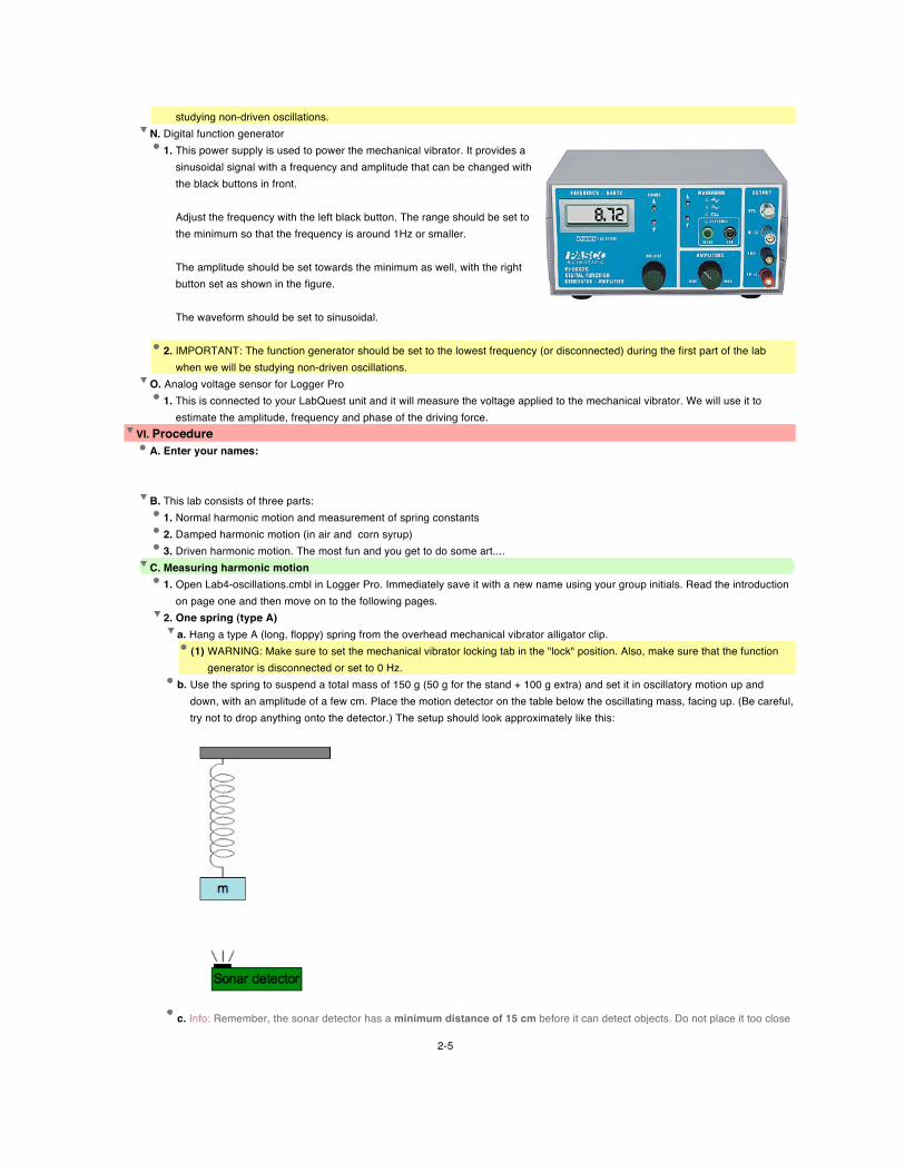
studying non-driven oscillations.N. Digital function generator

1. This power supply is used to power the mechanical vibrator. It provides a sinusoidal signal with a frequency and amplitude that can be changed with the black buttons in front.

Adjust the frequency with the left black button. The range should be set to the minimum so that the frequency is around 1Hz or smaller.

The amplitude should be set towards the minimum as well, with the right button set as shown in the figure.

The waveform should be set to sinusoidal.

2. IMPORTANT: The function generator should be set to the lowest frequency (or disconnected) during the first part of the lab when we will be studying non-driven oscillations.

O. Analog voltage sensor for Logger Pro1. This is connected to your LabQuest unit and it will measure the voltage applied to the mechanical vibrator. We will use it to

estimate the amplitude, frequency and phase of the driving force.VI. Procedure

A. Enter your names:

B. This lab consists of three parts:

1. Normal harmonic motion and measurement of spring constants2. Damped harmonic motion (in air and corn syrup)3. Driven harmonic motion. The most fun and you get to do some art....

C. Measuring harmonic motion1. Open Lab4-oscillations.cmbl in Logger Pro. Immediately save it with a new name using your group initials. Read the introduction

on page one and then move on to the following pages.2. One spring (type A)

a. Hang a type A (long, floppy) spring from the overhead mechanical vibrator alligator clip.(1) WARNING: Make sure to set the mechanical vibrator locking tab in the "lock" position. Also, make sure that the function

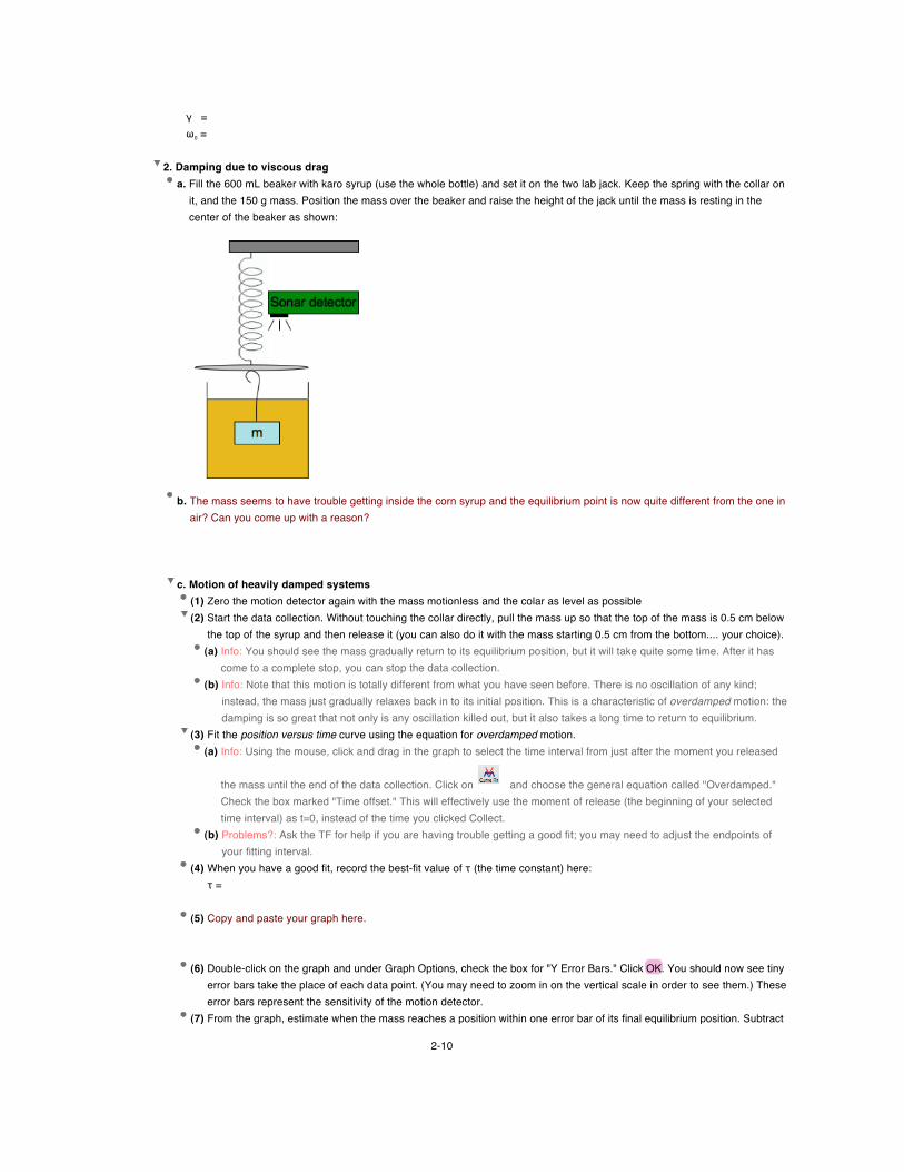
generator is disconnected or set to 0 Hz.b. Use the spring to suspend a total mass of 150 g (50 g for the stand + 100 g extra) and set it in oscillatory motion up and

down, with an amplitude of a few cm. Place the motion detector on the table below the oscillating mass, facing up. (Be careful, try not to drop anything onto the detector.) The setup should look approximately like this:

c. Info: Remember, the sonar detector has a minimum distance of 15 cm before it can detect objects. Do not place it too close

2-5

to your oscillating mass. Also, avoid using very large amplitudes of oscillation.d.

Start collecting data (click on ) and observe the mass's motion for a few periods. You should see a nice sinusoidal motion. (1) Problems?: If you don't see anything, you may need to re-scale the y-axis on the graph. If you see something more

complicated than a simple sine wave, you probably have an excessive amount of side-to-side motion in your oscillation. Try to get everything line up nice and vertical.

e. Try fitting a sinusoidal function to the position vs time graph.(1)

Info: Use the button and under "General equation," scroll down to the option near the bottom called "Undamped." (2) Problems?: If you can't find the "Undamped" function, you are using the wrong Logger Pro file!

f. Paste a copy of the position vs time graph, including the sinusoidal fit, below:

g. From your fit parameters, what is the angular frequency of the oscillation? (don't forget units):

Angular frequency (ω) =

h. From the value of ω, calculate the spring constant of the type A spring (don't forget units):kA =

3. Two B springs in seriesa. Now do the same thing with two type B springs. You'll need to use a larger mass because the B spring is much harder to

stretch; try a total mass of 550 g.b. Place two B springs in series (end-to-end) as shown:

c. Repeat the experiment, and calculate ω and keffective.(1) Paste a copy of the position vs time graph, including the sinusoidal fit, below:

(2) ω = (3) keffective = (4) Using what you learned from the pre-lab, calculate kB from the result above. Show and explain the calculation.

kB =

d. Does it seem like the two springs stretch by the same amount as the mass oscillates?

4. Three springs, in series/parallel

a. Connect one B and two A springs in the configuration shown below:

2-6

b. Before you actually measure anything, predict what value of keffective you would get from this combination. Explain.keffective,A (2 A springs in parallel) = keffective (3 springs) =

c. Now actually perform the experiment, using a mass of 250 g.(1) ω = (2) keffective =

(3) How well does this agree with your prediction? You don't need to make an error analysis but think about the possible

issues that can cause a discrepancy.

d. Compare the amount that spring B stretches with the amount that the A springs stretch. Are they equal? If not, which amount

is larger?

5. Something to think about

a. Suppose you took a type A spring and cut it in half, to make two shorter springs. What would the spring constant of one of these springs be?kA cut in half =

b. If you are curious, we have some half-A springs lying around for you to test your prediction.

6. OPTIONAL cross check. Do these ONLY after you have finished the lab and in case you are in doubt about your results above.a. Two A springs in parallel

(1) Now connect two type A springs in parallel (side-by-side) to suspend the same 150 g mass, like so:

2-7

(You'll need to put one end of each spring through the loop at the top, and one end of each through the hook on the mass stand. It's okay if the two springs are touching.)

(a) Problems?: If your sinusoidal function is not stable (for instance, it has a variable amplitude), wait a few moments for the motion to stabilize before taking your data. Also, try to get everything line up nice and vertical.

(2) Repeat the experiment, and calculate ω and keffective.(a) Paste a copy of the position vs time graph, including the sinusoidal fit, below:

(b) ω = (c) keffective =

(3) Compare this result to kA. Does this agree with what you found on the pre-lab?

b. One B spring(1) Now do the same thing for a single type B spring. You'll need to use a larger mass because the B spring is much harder to

stretch; try a total mass of 550 g.(2) Measure ω and calculate k for the type B spring:

(a) ω = (b) kB =

D. Exploring damping

1. Damping due to air draga. Now connect the spring with a "collar" to the mechanical vibrator and set up the sonar detector on the mounting unit above

the collar and facing down, as shown here. Use a mass of 150 g.

2-8

b. Zero the motion detector with the mass motionless at equilibrium and the collar as level as possible.(1)

Info: The detector is zeroed by clicking . It will click a few times and then be still.c. Set the oscillation going with a period of a few centimeters. Start collecting data and observe the motion of the mass over the

course of 15 or 20 seconds.(1) Info: You should notice that the mass still oscillates sinusoidally, but the amplitude gradually decreases over time. This is

because the collar has a significant amount of air drag, which provides a moderate amount of damping. (2) Problems?: If you see something more complicated and/or the amplitude is increasing and decreasing, you probably have

an excessive amount of side-to-side motion in your oscillation. Try to get everything line up nice and vertical, and wait a little for the motion to settle before taking your data.Also, make sure your sonar is positioned such that will get a good reading throughout the motion. If one side of the sinusoidal is cut, then your sonar is too close to the mass. Move the sonar further away.

d. Try fitting the curve called "Underdamped" to the position vs time graph.(1) This general function is a sine wave whose amplitude decreases exponentially with time:

position = A*exp(-t/B)*cos(C*t+D)+E.(2) Info: The key difference between this and undamped motion is the exponential factor, exp(-t/B). The parameter B is called

the time constant of the motion; it represents how quickly the amplitude decreases. The time constant is usually denoted with the Greek letter tau (τ), but Logger Pro doesn't do Greek letters in curve fitting, so that's why it's B in the equation.

(3) Info: In general, the time constant for damped motion depends on the amount of damping: for underdamped motion, increasing the amount of damping will cause the amplitude to decrease faster.

(4) Info: Quantitatively speaking, τ is equal to the amount of time it takes for the amplitude to decrease by a factor of 1/e, where e is the constant 2.718, the base of the natural logarithm. (1/e is about 0.37.)Here's a graph of exp(-t/τ) for τ=1.00 second:

e. Paste a copy of your position vs time graph, including the fit parameters, here:

f. What is the angular frequency of the oscillatory motion?ω =

g. What is the time constant for the motion?τ =

h. Looking at the graph, compare the amplitude of the motion at the beginning, and at a time B seconds later. Do they differ by a factor of about 2.7?

i. What is the damping constant and natural frequency of the system ω0? Tell us the equations to find these two quantities from

the results above and their values (you don't need to use greek letter!).

2-9

γ = ω0 =

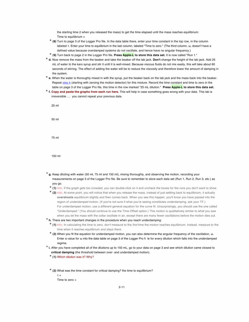
2. Damping due to viscous draga. Fill the 600 mL beaker with karo syrup (use the whole bottle) and set it on the two lab jack. Keep the spring with the collar on

it, and the 150 g mass. Position the mass over the beaker and raise the height of the jack until the mass is resting in the center of the beaker as shown:

b. The mass seems to have trouble getting inside the corn syrup and the equilibrium point is now quite different from the one in air? Can you come up with a reason?

c. Motion of heavily damped systems

(1) Zero the motion detector again with the mass motionless and the colar as level as possible(2) Start the data collection. Without touching the collar directly, pull the mass up so that the top of the mass is 0.5 cm below

the top of the syrup and then release it (you can also do it with the mass starting 0.5 cm from the bottom.... your choice).(a) Info: You should see the mass gradually return to its equilibrium position, but it will take quite some time. After it has

come to a complete stop, you can stop the data collection.(b) Info: Note that this motion is totally different from what you have seen before. There is no oscillation of any kind;

instead, the mass just gradually relaxes back in to its initial position. This is a characteristic of overdamped motion: the damping is so great that not only is any oscillation killed out, but it also takes a long time to return to equilibrium.

(3) Fit the position versus time curve using the equation for overdamped motion.(a) Info: Using the mouse, click and drag in the graph to select the time interval from just after the moment you released

the mass until the end of the data collection. Click on and choose the general equation called "Overdamped." Check the box marked "Time offset." This will effectively use the moment of release (the beginning of your selected time interval) as t=0, instead of the time you clicked Collect.

(b) Problems?: Ask the TF for help if you are having trouble getting a good fit; you may need to adjust the endpoints of your fitting interval.

(4) When you have a good fit, record the best-fit value of τ (the time constant) here:τ =

(5) Copy and paste your graph here.

(6) Double-click on the graph and under Graph Options, check the box for "Y Error Bars." Click OK. You should now see tiny

error bars take the place of each data point. (You may need to zoom in on the vertical scale in order to see them.) These error bars represent the sensitivity of the motion detector.

(7) From the graph, estimate when the mass reaches a position within one error bar of its final equilibrium position. Subtract

2-10

the starting time (t when you released the mass) to get the time elapsed until the mass reaches equilibrium:Time to equilibrium =

(8) Turn to page 3 of the Logger Pro file. In the data table there, enter your time constant in the top row, in the column labeled τ. Enter your time to equilibrium in the last column, labeled "Time to zero." (The third column, ω, doesn't have a defined value because overdamped systems do not oscillate, and hence have no angular frequency.)

(9) Turn back to page 2 in the Logger Pro file. Press Apple-L to store this data set. It is now called "Run 1."d. Now remove the mass from the beaker and take the beaker off the lab jack. Don't change the height of the lab jack. Add 25

mL of water to the karo syrup and stir it until it is well-mixed. Because viscous fluids do not mix easily, this will take about 60 seconds of stirring. The effect of adding the water will be to reduce the viscosity and therefore lower the amount of damping in the system.

e. When the water is thoroughly mixed in with the syrup, put the beaker back on the lab jack and the mass back into the beaker. Repeat step b (starting with zeroing the motion detector) for this mixture. Record the time constant and time to zero in the table on page 3 of the Logger Pro file, this time in the row marked "25 mL dilution." Press Apple-L to store this data set.

f. Copy and paste the graphs from each run here. This will help in case something goes wrong with your data. This lab is irreversible .... you cannot repeat your previous data.

25 ml

50 ml

75 ml

150 ml

g. Keep diluting with water (50 ml, 75 ml and 150 ml), mixing thoroughly, and observing the motion, recording your

measurements on page 3 of the Logger Pro file. Be sure to remember to store each data set (Run 1, Run 2, Run 3, etc.) as you go. (1) Info: If the graph gets too crowded, you can double-click on it and uncheck the boxes for the runs you don't want to show.(2) Info: At some point, you will notice that when you release the mass, instead of just settling back to equilibrium, it actually

overshoots equilibrium slightly and then comes back. When you see this happen, you'll know you have passed into the region of underdamped motion. (If you're not sure if what you're seeing constitutes underdamping, ask your TF.)For underdamped motion, use a different general equation for the curve fit. Unsurprisingly, you should use the one called "Underdamped." (You should continue to use the Time Offset option.) This motion is qualitatively similar to what you saw when you let the mass with the collar oscillate in air, except there are many fewer oscillations before the motion dies out.

h. There are two important changes in the procedure when you reach underdamping:(1) Info: In calculating the time to zero, don't measure to the first time the motion reaches equilibrium. Instead, measure to the

time when it reaches equilibrium and stays there.(2) When you fit the equation for underdamped motion, you can also determine the angular frequency of the oscillation, ω.

Enter a value for ω into the data table on page 3 of the Logger Pro fi le for every dilution which falls into the underdamped regime.

i. After you have completed all of the dilutions up to 150 mL, go to your data on page 3 and see which dilution came closest to critical damping (the threshold between over- and underdamped motion).(1) Which dilution was it? Why?

(2) What was the time constant for critical damping? the time to equilibrium?

τ = Time to zero =

2-11

(3) What is the damping constant γ and the natural frequency ω 0?(4) Re-fit the graph with the position versus time for the "critical damping" dilution using the "Critical damping" equation.

What is the damping constant γ and the natural frequency ω 0?γ = ω0 =

How do these compare with the values from the approximate equation?

(5) Create a graph showing both τ and Time to zero vs dilution and paste it here:

In words, what conclusions can you draw from this graph?

(a) Paste the table from page 3 of the Logger Pro file. To do this, you need to print the table to a pdf file.

Info: Highlight the table and go to the menu File -> Print Data Table .... Press "preview" in the print dialog. Then, select the table and copy and past it here.

(6) Look at the values of ω that you observed for the underdamped systems. How do they compare to the ω you got for the

same system damped only by air drag? For underdamped systems, does ω increase, decrease, or stay the same as the amount of damping goes up?

E. Driven harmonic motion

1. Now we are going to use the mechanical vibrator to drive the spring. We will do a few quick measurements to check how the system behaves in different conditions. There are no calculations in this part of the lab. You will only make plots and paste them below.

2. The groups on the left tables (facing the blackboard) should do this part of the lab with the corn syrup damping; the groups on the right should do it with air damping only.

3. Using the damped system with the corn syrup (only groups on the left side)a. Move the locking tab in the mechanical vibrator to the "unlocked" position. This will allow the vibrator to move.

Make sure the function generator is connected to the mechanical vibrator. Move to page 4 of the Logger Pro file.

b. First let's drive the system at the resonance frequency. That is the same natural frequency of the system that you found above.Enter the natural frequency here in rad/s and hertz: ω0 (rad/s) = f (Hertz) = (1) You will need to change the oscillation frequency of the vibrator by rotating the left button in the function generator. The

current frequency is displayed in the LCD monitor.(a) Info: You will likely have to tune the frequency a little above or below the frequency number above to find the

resonance frequency. Remember that at resonance the force and the position of the mass are 90 degrees out of phase.

(2) Copy and paste the plot of the position versus time and the plot of the position versus the force amplitude here. Comment.

Position versus time

Position versus potential

2-12

(a) Enter the resonance frequency here in hertz and compare with the natural frequency you had found for the system.

f (Hertz) =

c. Decrease the frequency by a factor of ~5 below the resonance frequency and repeat the same data taking.(1) Copy and paste the two plots here. Comment on your observations.

Position versus time

Position versus potential

d. Increase the frequency by ~50% relative to the resonance frequency.

(1) Copy and paste the two plots here. Comment on your observations.

Position versus time

Position versus potential

e. Finally, increase the frequency by a factor of ~5 relative to the resonance frequency.

(1) What do you observe? Look at the driver and the mass. Do you have an explanation?

(2) Copy and paste the position versus force plot here.

4. Using damping only by the air resistance (only groups on the right side)

a. Move the locking tab in the mechanical vibrator to the "unlocked" position. This will allow the vibrator to move.Make sure the function generator is connected to the mechanical vibrator. Move to page 4 of the Logger Pro file.

b. First let's drive the system at the resonance frequency. That is the same natural frequency of the system that you found above.Enter the natural frequency here in rad/s and hertz: ω0 (rad/s) = f (Hertz) = (1) You will need to change the oscillation frequency of the vibrator by rotating the left button in the function generator. The

current frequency is displayed in the LCD monitor.(a) Info: You will likely have to tune the frequency a little above or below the frequency number above to find the

resonance frequency. Remember that at resonance the force and the position of the mass are 90 degrees out of phase.

(2) Copy and paste the plot of the position versus time and the plot of the position versus the force amplitude here. Comment.

Position versus time

Position versus force

2-13

(a) Enter the resonance frequency here in hertz and compare with the natural frequency you had found for the system. f (Hertz) = 0.624

c. Decrease the frequency by a factor of ~5 below the resonance frequency and repeat the same data taking.(1) Copy and paste the two plots here. Comment on your observations.

Position versus time

Position versus potential

d. Increase the frequency by ~50% relative to the resonance frequency.

(1) Copy and paste the two plots here. Comment on your observations.

Position versus time

Position versus potential

e. Finally, increase the frequency by a factor of ~5 relative to the resonance frequency.

(1) What do you observe? Look at the driver and the mass. Do you have an explanation?

(2) Copy and paste the position versus force plot here.

F. Make some art

1. You might have noticed that some fancy patterns can be created with this setup. Try to create a nice one by changing the oscillation parameters, in particular the frequency of the function generator. You might want to take data for at least 60 sec or so.Paste it below:

VII. Conclusion

A. When you have finished, clean up anything in your work area that has has karo syrup all over it (the beaker, mass stand, masses, stirring rod, forceps if you used them, and anything else which was in the splash radius of your karo syrup) by taking it to the sink and rinsing it out thoroughly with warm water. Leave the glassware to dry on the tray at your station (not at the sink).

B. VERY IMPORTANT: Before leaving the lab, have your TF saving your report file into an USB pen. If he does not have your report, you will not get credit for the lab. Make sure your report file has your name on it.

2-14