lab #5: temperature and heat transfer

Lab #5: Temperature and Heat

Transfer

Introduction

Temperature is arguably the single most important abiotic factor influencing the physiology of an organism. Temperature is the average kinetic energy of a group of molecules. As temperature increases, the atoms and molecules that make up the structure of an organism vibrate and change position more quickly, and collide with one another more often and with more energy. As a result, the biochemistry that underpins virtually all aspects of structure and function in a living organism is influenced by its temperature. The temperature of an organism depends on a number of factors (e.g., specific heat capacity of the substances that make up the organism’s body, etc.), but the most important factor is the total heat (kinetic energy) content of the organism. Total heat content, in turn, depends on both heat production by an organism (though various heatproducing reactions that form part of its metabolism) and heat exchange with the surrounding environment.

Temperature reflects the ability of an object to transfer heat to another object in its surroundings. Based on the laws of thermodynamics, heat is transferred from object with a higher temperature to one with a lower temperature until a state of thermal equilibrium is reached. This transfer of heat typically occurs through four processes: conduction, convection, radiation, and evaporative cooling.

Conduction is the process of heat transfer between two bodies of matter that are adjacent to one another. Consider two objects at different temperatures in contact with one another. As the atoms in the object at a higher temperature vibrate they collide with atoms in the object at lower temperature, and kinetic energy (heat) is transferred to them. Thus heat

in the hotter object decreases (as does temperature) and that of the cooler object increases (as does temperature). The rate of conductive heat transfer between two objects can be expressed through a derivation of Fick’s Law:

𝐻 = 𝑘 × 𝑇2 − 𝑇1

𝑋

Where H is the rate of heat transfer (per unit cross sectional area), k is the thermal conductivity of the material through which heat is passing, X is the difference between two points, and T1 and T2 are the temperatures at the two respective points.

Rates of conductive heat loss can be reduced by insulating the surface with a material with low thermal conductivity. The blubber of marine mammals is an excellent example of such an insulator. The low conductivity of the lipids in the blubber compared to water restricts the transfer of heat from the body core to the surrounding water.

Convection is a condition where there is the macroscopic movement of a fluid (usually a liquid or gas) over an object. As heat is transferred between the surface of the object and the fluid, the heat is transferred by the physical relocation of the fluid. This greatly accelerates the transfer of heat between object and fluid above the rate at which it would occur through other processes such as convection. The rate of convective heat transfer can be expressed as follows:

𝐻 = ℎ𝑐 (𝑇𝑆 − 𝑇𝐹)

Where H is the rate of heat exchange be unit surface area, hc is the convection coefficient (which depends on flow rate, body shape, and orientation relative flow – higher flow rates and larger surfaces perpendicular to the direction of flow tend to increase this value), and TS and TF are the temperatures of the object surface and the fluid, respectively.

Rates of convective heat transfer can be

adjusted by an animal in numerous ways.

Orientation to the direction of flow can alter rates

of heat transfer. Insulating pelage, such as fur,

hair, or feathers, reduces the rate of flow at the

surface of the body and reduces the effects of

convection. Similarly, huddling behaviors in some

animals tend to break up the flow of the medium

over body surfaces.

Radiation, in contrast, is the transfer of heat in the form of electromagnetic radiation emanating from the surface of an object due to the thermal energy of matter above absolute zero. Unlike conduction, radiation can travel from one object to another without having matter in between the two objects. The total amount of radiation (as well as the range of wavelengths in the EM spectrum) emanating from an object increases as surface temperature increases in as described in the Stefan-Boltzmann Equation:

𝐻 = 𝜀𝜎𝑇𝑆 4

Where H is the rate of heat exchange per unit area, ε is the emissivity (the relative ability of a surface to emit radiation), σ in the Stefan-Boltzmann constant, and TS is the surface temperature of the object.

Radiant energy can be absorbed by an object, but can also be reflected from the object’s surface or simply pass through the object. The relative amount of radiant energy that does each depends on the object’s absorptivity, which is mathematically equal to its emissivity. This value is wavelength dependent – some wavelengths of electromagnetic radiation will tend to be absorbed, whereas others tend to be reflected or pass through the object. In the biosphere, most objects have similar emissivities and Stefan-Boltzmann constants at the typical infrared wavelengths (3000-4000 nm) that most objects produce at the temperatures prevalent on the planet’s surface. In such cases, the difference in

surface temperature between two objects is the principle factor influencing net radiant heat exchange (i.e., net radiant heat transfer occurs from the object with the hotter surface to that with the cooler surface). However, objects can vary considerably in their emissivity (an corresponding absorptivity) with respect to shorter wavelengths (e.g., visible light); those with high emissivities (and subsequently higher absorptivities) to certain wavelengths tend to absorb more of the radiation at those wavelengths and subsequently emit them at longer wavelengths, whereas those with low emissivities (and lower absorptivities) tend to reflect more of the radiation that strikes them. Thus the absorptive/reflective properties of an organism’s surface can influence radiant heat uptake from the sun (the only major source of short-wavelength radiation for much of the biosphere). Darker surfaces absorb more radiant heat, whereas lighter surfaces reflect more heat.

The final form of heat transfer between an object and its surroundings is evaporative cooling. Evaporative cooling occurs at the surface of an organism that as water on that surface converts from the liquid state to the vapor state. This phase transition absorbs a massive amount of heat (the latent heat of vaporization – roughly 570-595 cal/g water) from the surface of the animal and carries it away with the water vapor. This removal of heat from the surface of the animal can take place even if the temperature of the surrounding environment is equal to or even slightly higher than the body temperature of the animal.

Many terrestrial organisms employ evaporative cooling to regulate temperature, although this process results in water loss from the animal. Water vaporization (and the degree of cooling) is influenced by ambient temperature, the vapor pressure of the surrounding air, and convection.

Your Assignment… In today’s lab you will be conducting one of four experiments that will examine factors that influence

rates of heat exchange in model organisms. As objects placed in new thermal conditions heat or cool

toward an equilibrium temperature (Te) in curvilinear patterns, we will compare the effects of different

factors on heating and cooling by deriving the time constant τ (tau), which is the time needed for the

change in the temperature of the object toward equilibrium to reach 63.2% completion. Smaller values

of τ indicate a more rapid change in temperature.

Temperature recording and τ determination.

We will be using LabQuest digital datalogging interfaces to record

temperature from your models. Each interface can record data from three

or four different sensors (in this case thermistor probes) simultaneously.

During an experimental run, the probes will record temperature to the

nearest 0.1 °C every 0.1 sec so that we can precisely measure τ. The data will

be collected and graphically presented on the computers using LoggerPro

software.

1. Open the LoggerPro application on the

computer. The screen should appear

similar to the image to the right, with a

spreadsheet, a plot of temperature vs.

time, and live readouts for each of the

three thermistor probes. The size of

each of these objects can be adjusted

by clicking and dragging on the edges.

You should expand the spreadsheet

horizontally so that you can see the

columns for all three probes at the

same time. After adjusting the spreadsheet width, you may need to constrict the width of the

plot so that you can see the entire plot.

2. Click on “Experiment” in the menu bar at

the top, and select “Data Collection…”.

The Data Collection window will pop up.

Change the duration to 1200 seconds,

and the sampling rate to 10

samples/second.

3. When you are ready to start your data

recording, click on the “Collect” button

(the green arrow button at the top). The

program will begin recording

temperature readings in the spreadsheet

and plotting those values on the plot.

In many cases we will not know a priori

what the equilibrium temperature of the

measurements will be. Monitor the

change in temperature in the

spreadsheet. We will assume that Teq is

reached when the same temperature

reading is sustained for >30 seconds.

Once you have reached Teq for all three probes, click on the “Stop” button at the top.

4. Determine the initial temperature (Ti) for each model. This will be the LOWEST temperature

recorded in your data set and should be at or near the beginning of the recordings.

5. Calculate the difference between Ti and Teq. Multiply this value by 0.632, then add this value to

Ti. This will be the temperature at which 63.2% of the total change in temperature is reached.

From your data set for each model, determine how much time from Ti elapsed to reach this

temperature -- this is the value of τ.

Group A – Effect of evaporative cooling and convection on heat loss.

I. Sample preparation

You will receive a set of foam rubber sponges each with a small tunnel drilled through its center for

insertion of a thermocouple probe. The sponges will be heated in a 40 °C incubator. Assign six (6)

sponges per experimental group. The datalogging systems can record temperature in three sponges

simultaneously, so you will only need to do two runs for each group.

• Dry, still air - insert the thermistor probe to the center of the sponge. Place the sponge on an

inverted lid for a small jar, then place the inverted jar on top to cover the sponge. Once all five

sponges are ready, place the inverted jars into the incubators, remove the jars to expose the

sponges, close the incubator, and begin recording with the data logging system.

• Wet, still air – after completing measurements for the dry sponges, remove them from the

incubators and give them a few squeezes to help drop them down to near room temperature.

You will then dampen the sponges with the following procedure: (1) transfer 5 ml of room –

temperature water into a beaker, (2) remove the sponge from the oven and compress the

sponge into the water to absorb as much water as possible, (3) squeeze and release the sponge

several times to distribute the volume of water throughout the sponge. Once a sponge is

dampened, insert the thermocouple probe to the center of the sponge. Place the sponge on an



sponges, close the incubator, and begin recording with the data logging system.

• Dry, convection – obtain a second set of dry sponges. Insert the thermistor probe to the center

of the sponge. Place the sponge on an inverted lid for a small jar, then place the inverted jar on

top to cover the sponge. Once all five sponges are ready, place the inverted jars into the

incubators, remove the jars to expose the sponges, close the incubator, turn on the air pump to

circulate the air in the incubator (1 L/min), and begin recording with the data logging system.

• Wet, convection - after completing measurements for the dry sponges, remove them from the

incubators and give them a few squeezes to help drop them down to near room temperature.

You will then dampen the sponges with the following procedure: (1) transfer 5 ml of room –

temperature water into a beaker, (2) remove the sponge from the oven and compress the

sponge into the water to absorb as much water as possible, (3) squeeze and release the sponge

several times to distribute the volume of water throughout the sponge. Once a sponge is

dampened, insert the thermocouple probe to the center of the sponge. Place the sponge on an



sponges, close the incubator, turn on the air pump to circulate the air in the incubator (1 L/min),

and begin recording with the data logging system.

Data Analysis for Group A

Determination of τ – We do not know a priori what the equilibrium temperature of the

measurements will be. Here, we will consider the equilibrium temperature reached when the same

value is given for four consecutive temperature readings. Record this value. Once the equilibrium

temperature is determined, calculate the difference between the initial temperature (the first

reading) and the equilibrium temperature. Multiply this value by 0.632, then add this value to the

initial temperature. This will be the temperature at which 63.2% of the total change in temperature

is reached. From your data set for each sponge, determine how much time elapsed to reach this

temperature: this will be the value of τ. Record this value for each sponge.

ANOVA - You will conduct an Analysis of Variance (ANOVA) to evaluate the effects of evaporative

water loss and convection on both Equilibrium Temperature (Te) and the time constant (τ).

1. Open up SPSS and select “Type in Data”. This will open a blank spread sheet

2. In the bottom-left corner of the window there is a button titled “Variable View”. Click on

that button

3. In Row 1, under “Name”, type “WETDRY”, then click the cell next to it under “Type”. It will

automatically enter “Numerical” but there is a button to the right of this word with three

periods in it. Click on that button and select “String”.

4. In Row 2, under “Name”, type “AIRFLOW”, then click the cell next to it under “Type”. Once

again, set the type of data to be entered as “String”.

5. In Row 3, type in “Te” as the name. Leave the data type as “Numerical”

6. In Row 4, type in “Tau” as the name, and again leave the data type as “Numerical”

7. Now click the “Data View” button in the

bottom-left corner of the window. Notice that

the different variables you just entered are now

the column headings. Enter in your data for

each sponge. For “WETDRY”, indicate if the

sponge is “WET” or “DRY”. For “WIND”,

indicate if the air was “STILL” or “BLOWING”.

Enter in the respective Te and Tau values in the

last two columns.

8. From the menu at the top select Analyze

→General Linear Model → Univariate… This

will bring up a small window (“Univariate”).

9. Assign ”Te” as your dependent variable and

both “WETDRY” and “WIND” as fixed factors,

then click on the “Model” button at the upper

right. A new window (“Univariate Model”) will

pop open.

10. Select “Custom” and then assign the variables

to the model. First click on “WETDRY” in the

column to the left and then the button at the

center to assign it, then click on “WIND” and

similarly assign it to the model. Finally click

on “WETDRY” then, holding the CTRL key

down, click on “WIND”. Both will be

highlighted at the same time. Click on the

arrow button to assign a “WETDRY*WIND”

interaction term to the model. Click Continue

to go back to the “Univariate” window.

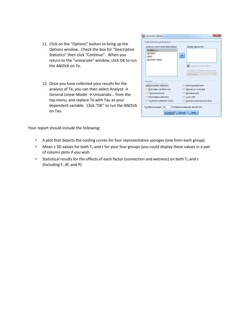
11. Click on the “Options” button to bring up the

Options window. Check the box for “Descriptive

Statistics” then click “Continue”. When you

return to the “univariate” window, click OK to run

the ANOVA on Te.

12. Once you have collected your results for the

analysis of Te, you can then select Analyze →

General Linear Model → Univariate… from the

top menu, and replace Te with Tau as your

dependent variable. Click “OK” to run the ANOVA

on Tau.

Your report should include the following:

• A plot that depicts the cooling curves for four representative sponges (one from each group).

• Mean ± SD values for both Te and τ for your four groups (you could display these values in a pair

of column plots if you wish

• Statistical results for the effects of each factor (convection and wetness) on both Te and τ

(Including F, df, and P)

Group B – Effect of color on radiant heating

You will be provided with a set “model organisms” constructed from metal pipe and painted different

colors (white or black). You will measure both surface temperatures and core body temperatures for

each during the experiment as the organisms heat under either a heating bulb (which emits mostly long

wavelength EM radiation) or a full spectrum plant bulb (which emits more short wavelength EM

radiation).

1. Insert the thermistor probe into the center of the model organism.

2. Place the model organism on the test rack below the IR temperature probe clamped to the ring

stand. The position of the model organism relative to the IR probe must be the same each time.

3. A shop lamp holding the plant bulb will be clamped into position next to the apparatus. Plug the

lamp into the rheostat (voltage regulator) provided.

4. When ready, switch on the lamp, and begin recording both surface and core temperature using

the datalogging system.

5. Once you have completed measurements on all experimental organisms with the plant bulb,

replace the shop lamp with the one that holds a heating lamp bulb, and repeat the experiment

with each of the model organisms.

Determination of τ – Note that the surface and core temperatures may reach equilibrium at

different times. Once the equilibrium temperature is determined, calculate the difference between

the initial temperature (the first reading) and the equilibrium temperature. Multiply this value by

0.632, then add this value to the initial temperature. This will be the temperature at which 63.2% of

the total change in temperature is reached. Determine how much time elapsed to reach this

temperature: this will be the value of τ.

ANOVA - You will conduct an Analysis of Variance (ANOVA) to evaluate the effects of color and

radiation source (long wavelength or short wavelength) on Equilibrium Temperatures (Te) and the

time constants (τ) both at the surface and in the body core of the test animals.



that button

3. In Row 1, under “Name”, type “COLOR”, then click the cell next to it under “Type”. It will



4. In Row 2, type in “Te-Surface” as the name. Leave the data type as “Numerical”

5. In Row 3, type in “Tau-Surface” as the name, and again leave the data type as “Numerical”

6. In Row 4, type in “Te-Core” as the name. Leave the data type as “Numerical”

7. In Row 5, type in “Tau-Core” as the name, and again leave the data type as “Numerical”

8. Now click the “Data View” button in the bottom-left corner of the window. Notice that the

different variables you just entered are now the column headings. Enter in your data for

each model. For “COLOR”, indicate if the model is “BLACK” or “WHITE”. Enter in the Te and

Tau values for the surface and the core in the respective remaining columns.

9. From the menu at the top select Analyze →

General Linear Model → Univariate… This will

bring up a small window (“Univariate”).

10. Assign ”Te-surface” as your dependent variable

and “COLOR” as your fixed factor, then click on

the “Model” button at the upper right. A new

window (“Univariate Model”) will pop open.

11. Select “Custom” and then assign the variables to the

model. First click on “COLOR” in the column to the

left and then the button at the center to assign it.

Click “Continue” to go back to the “Univariate”

window.


Options window. Check the box for “Descriptive

Statistics” then click “Continue”. When you return

to the “univariate” window, click OK to run the

ANOVA on Te-Surface.

13. Once you have collected your results for the analysis of Te-surface, you can then select

Analyze → General Linear Model → Univariate… from the top menu, and replace Te-surface

with Tau-surface as your dependent variable. Click “OK” to run the ANOVA on Tau-surface.

14. Repeat the above step, replacing Tau-surface with Te-core as the dependent variable.

15. Repeat the above step, replacing Te-core with Tau core as the dependent variable.


• A plot that depicts the heating curves for four representative models (one from each group).

• Mean ± SD values for Te and τ for both surface and core readings in each your four groups (you

could display these values in a pair of column plots if you wish).

• Statistical results for the effects of color on both Te and τ for the surface and the body core

(Including F, df, and P).

Group C - Effects of pelage and flow rate on convective heat transfer

You will be provided with a set “model organisms” constructed from metal pipe that are either bare or

covered with insulating “pelage”. You will measure core body temperatures for each during the

experiment as the organisms cool under different rates of air flow.

1. Record air temperature on the test rack.

2. Remove the model organism from its incubator (40 °C) and insert the thermocouple probe into

the center.

3. Place the model organism on the test rack perpendicular to the outflow nozzle for the air pump.

The air pump is plugged into a rheostat that will allow us to adjust the flow rate.

4. With the air pump turned off, begin recording body temperature using the datalogging system.

5. Return the organism to the incubator after completion, and repeat with the other organisms

6. Once still-air recordings for each model have been obtained, set the dial on the rheostat to 60 V.

insert the probe back into one of the model organisms, place it on the test rack, switch on the

power to air pump through the rheostat, and begin recording body temperature until the

equilibrium temperature (room temperature) is reached. Repeat with each model. Once the

last model organism is completed, measure and record the flow rate of air from the flow meter.

7. Once low rate airflow recordings for each model have been obtained, turn up the dial on the

rheostat to 120 V. Insert the probe back into one of the model organisms, place it on the test

rack, switch on the power to air pump through the rheostat, and begin recording body

temperature until the equilibrium temperature (room temperature) is reached. Repeat with

each model. Once the last model organism is completed, measure and record the flow rate of

air from the flow meter.

Determination of τ – In this experiment, the final (equilibrium) temperature should be equal to room

temperature. Calculate the difference between the initial temperature (first reading) of each model

and room temperature. Multiply this difference by 0.632 and add to the initial temperature to

determine the temperature at which the model has reached 63.2% completion. Determine the time

elapsed to reach this temperature from your data set– this will be the value of τ.

ANOVA - You will conduct an Analysis of Variance (ANOVA) to evaluate the effects of insulation and

convective flow rate on the time constant (τ).



that button

3. In Row 1, under “Name”, type “PELAGE”, then click the cell next to it under “Type”. It will



4. In Row 2, under “Name”, type “FLOW”, then click the cell next to it under “Type”. Once

again, set the type of data to be entered as “String”.

5. In Row 3, type in “Tau” as the name, and again leave the data type as “Numerical”

6. Now click the “Data View” button in the bottom-left corner of the window. Notice that the

different variables you just entered are now the column headings. Enter in your data for

each model. For “PELAGE”, indicate if the model is “BARE” or “FUZZY”. For “FLOW”, enter

the flow rate from the flow meter (enter 0 for still air). Enter in the Tau values for each

model in the remaining columns.


General Linear Model → Univariate… This will

bring up a small window (“Univariate”).

8. Assign ”Te-surface” as your dependent

variable as both “PELAGE” and “FLOW” as

fixed factors, then click on the “Model” button

at the upper right. A new window (“Univariate

Model”) will pop open.

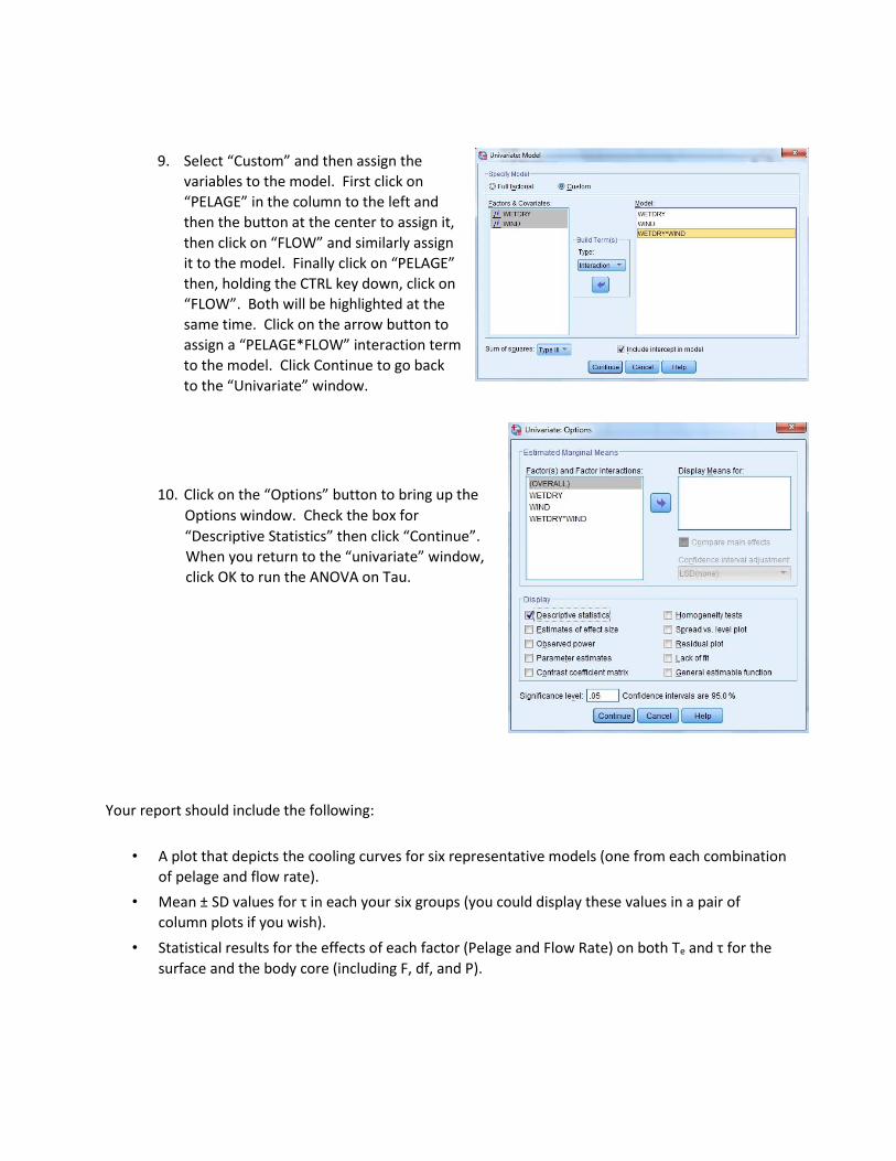
9. Select “Custom” and then assign the

variables to the model. First click on

“PELAGE” in the column to the left and

then the button at the center to assign it,

then click on “FLOW” and similarly assign

it to the model. Finally click on “PELAGE”

then, holding the CTRL key down, click on

“FLOW”. Both will be highlighted at the

same time. Click on the arrow button to

assign a “PELAGE*FLOW” interaction term

to the model. Click Continue to go back

to the “Univariate” window.


Options window. Check the box for

“Descriptive Statistics” then click “Continue”.

When you return to the “univariate” window,

click OK to run the ANOVA on Tau.


• A plot that depicts the cooling curves for six representative models (one from each combination

of pelage and flow rate).

• Mean ± SD values for τ in each your six groups (you could display these values in a pair of

column plots if you wish).

• Statistical results for the effects of each factor (Pelage and Flow Rate) on both Te and τ for the

surface and the body core (including F, df, and P).

Group D – Effects of environmental temperature and body size on conductive heating

In this experiment you will place cube-shaped model organisms of different sizes into water baths of

three different temperatures and monitor changes in core body temperature. There are four different

sized models that are roughly isometric in terms of their linear dimensions.

1. Select a set of four different sized models. Weigh each, and measure its length and diameter

with a ruler or pair of calipers.

2. Insert one of the thermistor probes into the center of one end of each of the models and push

through to the center of the model. Return to the ice bath to cool.

3. When ready, remove from the ice bath and transfer all five models simultaneously to the 32 °C

water bath.

4. Begin recording temperatures using the datalogging software. Continue recording until all four

models reach the equilibrium temperature (I,e,, the bath temperature).

5. Repeat the experiment with a second group of models – this time transferring them into a 42 °C

water bath.

6. Repeat the experiment with a third group of models – this time transferring them into a 22 °C

water bath.





elapsed to reach this temperature from your data set – this will be the value of τ.

Calculation of Surface Area – Calculate the total surface area of each model as follows:

𝑆A = 6 × 𝑙2

Where l is the length of the model on one side.

ANCOVA - You will conduct Analyses of Covariance (ANCOVA) to evaluate the effects of body mass,

surface area and the time constant (τ).



that button

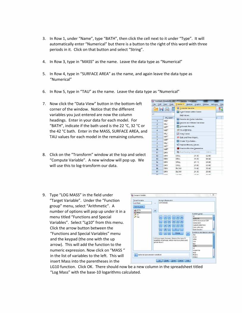
3. In Row 1, under “Name”, type “BATH”, then click the cell next to it under “Type”. It will



4. In Row 3, type in “MASS” as the name. Leave the data type as “Numerical”

5. In Row 4, type in “SURFACE AREA” as the name, and again leave the data type as

“Numerical”

6. In Row 5, type in “TAU” as the name. Leave the data type as “Numerical”

7. Now click the “Data View” button in the bottom-left

corner of the window. Notice that the different

variables you just entered are now the column

headings. Enter in your data for each model. For

“BATH”, indicate if the bath used is the 22 °C, 32 °C or

the 42 °C bath. Enter in the MASS, SURFACE AREA, and

TAU values for each model in the remaining columns.

8. Click on the “Transform” window at the top and select

“Compute Variable”. A new window will pop up. We

will use this to log-transform our data.

9. Type “LOG MASS” in the field under

“Target Variable”. Under the “Function

group” menu, select “Arithmetic”. A

number of options will pop up under it in a

menu titled “Functions and Special

Variables”. Select “Lg10” from this menu.

Click the arrow button between the

“Functions and Special Variables” menu

and the keypad (the one with the up

arrow). This will add the function to the

numeric expression. Now click on “MASS “

in the list of variables to the left. This will

insert Mass into the parentheses in the

LG10 function. Click OK. There should now be a new column in the spreadsheet titled

“Log Mass” with the base-10 logarithms calculated.

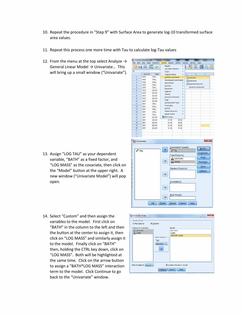
10. Repeat the procedure in “Step 9” with Surface Area to generate log-10 transformed surface

area values.

11. Repeat this process one more time with Tau to calculate log-Tau values


General Linear Model → Univariate… This


13. Assign ”LOG TAU” as your dependent

variable, “BATH” as a fixed factor, and

“LOG MASS” as the covariate, then click on

the “Model” button at the upper right. A

new window (“Univariate Model”) will pop

open.



“BATH” in the column to the left and then

the button at the center to assign it, then

click on “LOG MASS” and similarly assign it

to the model. Finally click on “BATH”

then, holding the CTRL key down, click on

“LOG MASS”. Both will be highlighted at

the same time. Click on the arrow button

to assign a “BATH*LOG MASS” interaction

term to the model. Click Continue to go

back to the “Univariate” window.





click OK to run the ANOVA on LOG TAU.


analysis of Log Tau with Log Mass as the

covariate, you can then select Analyze →


top menu, and replace LOG MASS with LOG

SURFACE AREA as your covariate. Click “OK”

to run the ANCOVA


• A plot that depicts the heating curves for all four models in one of the baths (specify which

temperature).

• A plot of log τ (sec) vs. log mass (g) for each of the three temperatures. Generate a linear

regression for each of the two data sets. The slope of this line indicates the scaling relationship.

• A plot of log τ (sec) vs. log surface area (cm) for each of the three temperatures. Once again,

generate a linear regression for each data set and determine the scaling relationship.

• Statistical results evaluating whether bath temperature and/or size influence τ.

Group E – Effects of initial body temperature and body size on conductive cooling

In this experiment you will place cube-shaped model organisms of different sizes with three different

starting temperatures into a single refrigeration bath and monitor changes in core body temperature.

There are four different sized models that are roughly isometric in terms of their linear dimensions.

7. Select a set of four different sized models. Weigh each, and measure its length and diameter

with a ruler or pair of calipers.

8. Insert one of the thermistor probes into the center of one end of each of the models and push

through to the center of the model. Return to the ice bath to cool.

9. When ready, remove from the ice bath and transfer all five models simultaneously to the 32 °C

water bath.

10. Begin recording temperatures using the datalogging software. Continue recording until all four

models reach the equilibrium temperature (I,e,, the bath temperature).

11. Repeat the experiment with a second group of models – this time transferring them into a 42 °C

water bath.

12. Repeat the experiment with a third group of models – this time transferring them into a 22 °C

water bath.





elapsed to reach this temperature from your data set – this will be the value of τ.

Calculation of Surface Area – Calculate the total surface area of each model as follows:

𝑆A = 6 × 𝑙2

Where l is the length of the model on one side.

ANCOVA - You will conduct Analyses of Covariance (ANCOVA) to evaluate the effects of body mass,

surface area and the time constant (τ).



that button

3. In Row 1, under “Name”, type “ITEMP” (for “initial temperature), then click the cell next to it

under “Type”. It will automatically enter “Numerical” but there is a button to the right of

this word with three periods in it. Click on that button and select “String”.

4. In Row 3, type in “MASS” as the name. Leave the data type as “Numerical”

5. In Row 4, type in “SURFACE AREA” as the name, and again leave the data type as

“Numerical”

6. In Row 5, type in “TAU” as the name. Leave the data type as “Numerical”

7. Now click the “Data View” button in the bottom-left

corner of the window. Notice that the different

variables you just entered are now the column

headings. Enter in your data for each model. For

“ITEMP”, indicate if starting temperature was 22 °C, 32

°C or 42 °C. Enter in the MASS, SURFACE AREA, and

TAU values for each model in the remaining columns.

8. Click on the “Transform” window at the top and select

“Compute Variable”. A new window will pop up. We

will use this to log-transform our data.

9. Type “LOG MASS” in the field under

“Target Variable”. Under the “Function

group” menu, select “Arithmetic”. A

number of options will pop up under it in a

menu titled “Functions and Special

Variables”. Select “Lg10” from this menu.

Click the arrow button between the

“Functions and Special Variables” menu

and the keypad (the one with the up

arrow). This will add the function to the

numeric expression. Now click on “MASS “

in the list of variables to the left. This will

insert Mass into the parentheses in the

LG10 function. Click OK. There should now be a new column in the spreadsheet titled

“Log Mass” with the base-10 logarithms calculated.

10. Repeat the procedure in “Step 9” with Surface Area to generate log-10 transformed surface

area values.

11. Repeat this process one more time with Tau to calculate log-Tau values


General Linear Model → Univariate… This


13. Assign ”LOG TAU” as your dependent

variable, “ITEMP” as a fixed factor, and

“LOG MASS” as the covariate, then click on

the “Model” button at the upper right. A

new window (“Univariate Model”) will pop

open.



“ITEMP” in the column to the left and

then the button at the center to assign it,

then click on “LOG MASS” and similarly

assign it to the model. Finally click on

“ITEMP” then, holding the CTRL key down,

click on “LOG MASS”. Both will be

highlighted at the same time. Click on the

arrow button to assign a “ITEMP*LOG

MASS” interaction term to the model.

Click Continue to go back to the “Univariate” window.





click OK to run the ANOVA on LOG TAU.


analysis of Log Tau with Log Mass as the

covariate, you can then select Analyze →


top menu, and replace LOG MASS with LOG

SURFACE AREA as your covariate. Click “OK”

to run the ANCOVA


• A plot that depicts the cooling curves for all four models at one starting temperature (specify

which temperature).

• A plot of log τ (sec) vs. log mass (g) for each of the three initial temperatures. Generate a linear

regression for each of the two data sets. The slope of this line indicates the scaling relationship.

• A plot of log τ (sec) vs. log surface area (cm) for each of the three initial temperatures. Once

again, generate a linear regression for each data set and determine the scaling relationship.

• Statistical results evaluating whether initial temperature and/or size influence τ.

lab #5: temperature and heat transfer

Documents