REPORT ON LABORATORY

MIX DESIGN

Date of Submission: 25th September 2013

Experiment no.1:

To determine the physical properties of fine and coarse aggregate and prepare the mix design for M20 grade of concrete.

Objective:

To study the physical properties of fine and coarse aggregate

To find the grading of both types of aggregate.

To produce different grade of concrete by trial mixing.

Theory:The specific gravity of coarse and fine aggregate were to needed for mix design along

with grading of both types of aggregates. For mix design IS method is followed.

General Procedure of Mix Design

1.0 GeneralA comprehensive trial mixing comprises i) collection of representative samples of materials from the sources or stockpiles, ii) Various tests on the individual samples in the laboratory and iii) trial mixing for workability and compressive strengths. The materials in question are i) Cement ii) Coarse Aggregate iii) Fine Aggregate and iv) Water for use in concrete, (provisional).

2.0 Cement: Cement Samples are to be delivered to the laboratory in unbroken bags. Preferably, the cement samples should come straight from the factory.

The tests to be conducted on cement are the following:a. Consistency and setting times (initial and final)b. Fineness of cement, by Blaine Apparatus c. Specific Gravityd. Soundness e. Standard Mortar Cube Strength to determine 3, 7 and 28 days strength.

3.0 Coarse Aggregate:Coarse aggregate are crushed aggregate which are lots based on the nominal size 20.

In case of crushed aggregate, samples are collected during production at crusher site. Natural aggregate sample should be collected from the stockpiles or heaps after plant or manual screening.

The tests to be conducted on the coarse aggregate are:a. Particle Size Distribution or Sieve Analysisb. Specific Gravities and Water Absorption c. Flakiness Index

2

d. Elongation Index

4.0 Fine Aggregate:Normally, fine aggregate are natural sand from river bed or pits (quarry).Samples are to be collected from stockpiles or heaps after screening and/or washing as necessary.

The tests to be conducted are:a. Sieve Analysis ( for particle size distribution and to determine Fineness Modulus)b. Specific Gravity and Absorption

5.0 Water:The tests to be conducted are:1. Chemical Test to determine chloride content etc. 2. Trial Mixers to compare strength with those of the mixes made with distilled water.

(Normally, if potable water is used for concrete, no tests are required). Other than the above, the project specification may require additional tests.

6.0 Trial Mixing

6.1.1 Given Condition:

The client should provide the following information.a. Type of specimen whether cylinder or cube b. Grade of concrete in terms of minimum strength at 28 days.c. Nominal size of aggregated. Type of aggregate – natural or crushede. Desired Workability – Slumpf. Method of Batching at site- whether volumetric or by weight

6.1.2 Design Strength:

Design strength, which should always be more than the minimum strength, is estimated as follows.

fd= fck + K*

Where, fd = design strength or target strengthfck = Minimum Specified StrengthK = a value representing number of standard deviation units along the abscissa of

a normal distribution curve, that determines the percentage of tests on concrete specimens to record strength above the minimum ( Normally, K =1.65 for 95% of the tests to record strengths higher than the minimum specified strength)

3

= Standard Deviation, which is either assumed at the beginning or estimated on the basis of degree of control at site, which depend mostly on the method of batching the ingredients, volumetric or by weight and the quality of supervision.

Standard Deviation () can be obtained from the relationship:

Co-efficient of variation Cv = Standard Deviation/Meani.e. Cv = /fd (Here the design strength is considered as mean strength)

Normally the value of Cv is between 0.12 for “excellent” to 0.18 “Fair” degree of control.

Cv = 0.12 for mixing concrete in a batching plant= 0.15 for weight batching on a portable mixer= 0.18 for volumetric batching in a portable mixer

6.2 Tentative Mix Proportions for Trial Mixing

Having tested all the materials as stated above and having been given the client’s requirement of strength and workability, trial mix proportions are computed for different water cement ratios. From the sieve analysis result of coarse and fine aggregate a best combined grading is formulated. (A separate trail mixes may be carried out for slump tests only to determine the actual quantity of mixer water required for the desired workability).

6.3 Trial Mixing

The mix proportion is based on “Saturated Surface Dry” condition of coarse and fine aggregate. The aggregate will have to be soaked in water for sufficient time and the surface water wiped off and air- dried if necessary to bring the aggregate to a “SSD’ condition.

Mixing will be done in a “Pan-type” laboratory mixer; workability will be measured and the specimens, cylinder or cube, will be cast. Nine numbers each of specimens will be prepared for each w/c ratio.

3 Each specimen is tested for 3 –day, 7 –day and 28 day strength. This will also give idea of the strength development characteristics.

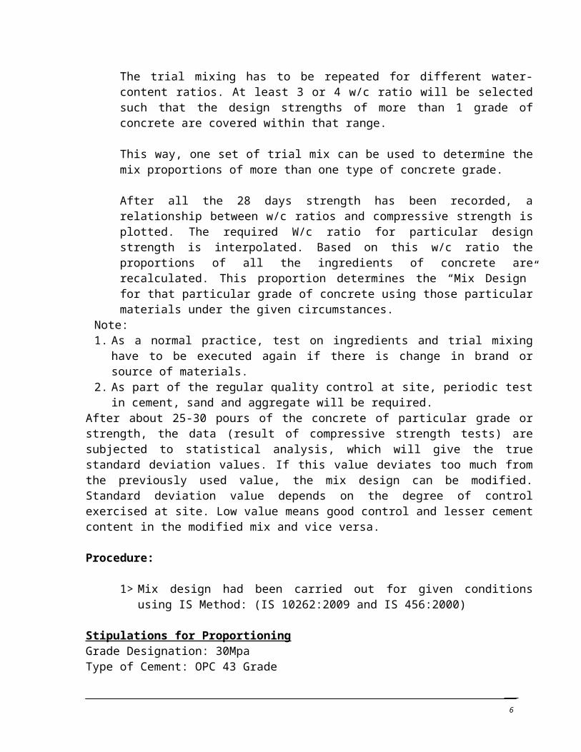
The trial mixing has to be repeated for different water-content ratios. At least 3 or 4 w/c ratio will be selected such that the design strengths of more than 1 grade of concrete are covered within that range.

This way, one set of trial mix can be used to determine the mix proportions of more than one type of concrete grade.

4

After all the 28 days strength has been recorded, a relationship between w/c ratios and compressive strength is plotted. The required W/c ratio for particular design strength is interpolated. Based on this w/c ratio the proportions of all the ingredients of concrete are recalculated. This proportion determines the “Mix Design” for that particular grade of concrete using those particular materials under the given circumstances.

Note: 1. As a normal practice, test on ingredients and trial mixing have to be executed again if there

is change in brand or source of materials. 2. As part of the regular quality control at site, periodic test in cement, sand and aggregate will

be required.After about 25-30 pours of the concrete of particular grade or strength, the data (result of compressive strength tests) are subjected to statistical analysis, which will give the true standard deviation values. If this value deviates too much from the previously used value, the mix design can be modified. Standard deviation value depends on the degree of control exercised at site. Low value means good control and lesser cement content in the modified mix and vice versa.

Procedure:

1> Mix design had been carried out for given conditions using IS Method: (IS 10262:2009 and IS 456:2000)

Stipulations for ProportioningGrade Designation: 30MpaType of Cement: OPC 43 GradeExposure: Moderate (Reinforced Concrete)Nominal maximum size of aggregate: 20mmMinimum cement content: 300 Kg/m3

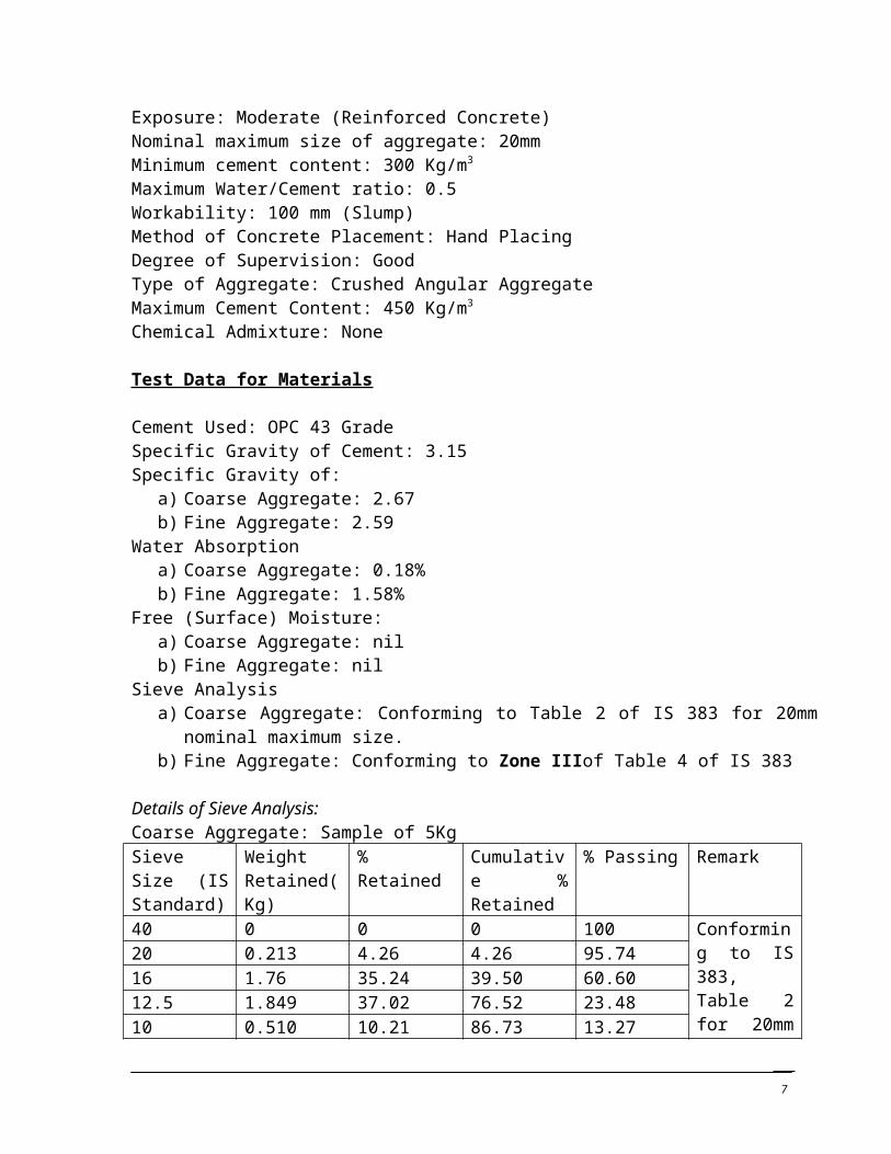
Maximum Water/Cement ratio: 0.5Workability: 100 mm (Slump)Method of Concrete Placement: Hand PlacingDegree of Supervision: GoodType of Aggregate: Crushed Angular AggregateMaximum Cement Content: 450 Kg/m3

Chemical Admixture: None

Test Data for Materials

Cement Used: OPC 43 GradeSpecific Gravity of Cement: 3.15Specific Gravity of:

a) Coarse Aggregate: 2.67b) Fine Aggregate: 2.59

Water Absorptiona) Coarse Aggregate: 0.18%b) Fine Aggregate: 1.58%

Free (Surface) Moisture:

5

a) Coarse Aggregate: nilb) Fine Aggregate: nil

Sieve Analysisa) Coarse Aggregate: Conforming to Table 2 of IS 383 for 20mm nominal maximum size.b) Fine Aggregate: Conforming to Zone IIIof Table 4 of IS 383

Details of Sieve Analysis:Coarse Aggregate: Sample of 5KgSieve Size (IS Standard)

Weight Retained(Kg)

% Retained Cumulative % Retained

% Passing Remark

40 0 0 0 100 Conforming to IS 383, Table 2 for 20mm Nominal Maximum size.

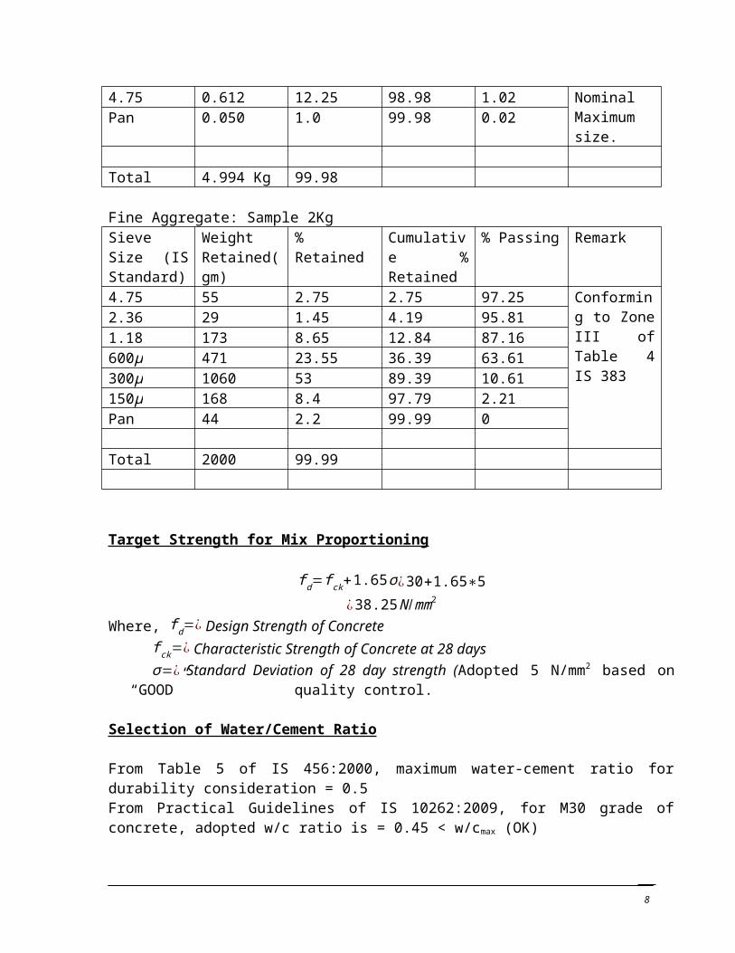
20 0.213 4.26 4.26 95.7416 1.76 35.24 39.50 60.6012.5 1.849 37.02 76.52 23.4810 0.510 10.21 86.73 13.274.75 0.612 12.25 98.98 1.02Pan 0.050 1.0 99.98 0.02

Total 4.994 Kg 99.98

Fine Aggregate: Sample 2KgSieve Size (IS Standard)

Weight Retained(gm)

% Retained Cumulative % Retained

% Passing Remark

4.75 55 2.75 2.75 97.25 Conforming to Zone III of Table 4 IS 383

2.36 29 1.45 4.19 95.811.18 173 8.65 12.84 87.16600μ 471 23.55 36.39 63.61300μ 1060 53 89.39 10.61150μ 168 8.4 97.79 2.21Pan 44 2.2 99.99 0

Total 2000 99.99

Target Strength for Mix Proportioning

f d=f ck+1.65 σ¿30+1.65∗5

¿38.25 N /mm2

Where, f d=¿ Design Strength of Concretef ck=¿ Characteristic Strength of Concrete at 28 daysσ=¿ Standard Deviation of 28 day strength (Adopted 5 N/mm2 based on “GOOD”

quality control.

Selection of Water/Cement Ratio

6

From Table 5 of IS 456:2000, maximum water-cement ratio for durability consideration = 0.5From Practical Guidelines of IS 10262:2009, for M30 grade of concrete, adopted w/c ratio is = 0.45 < w/cmax (OK)

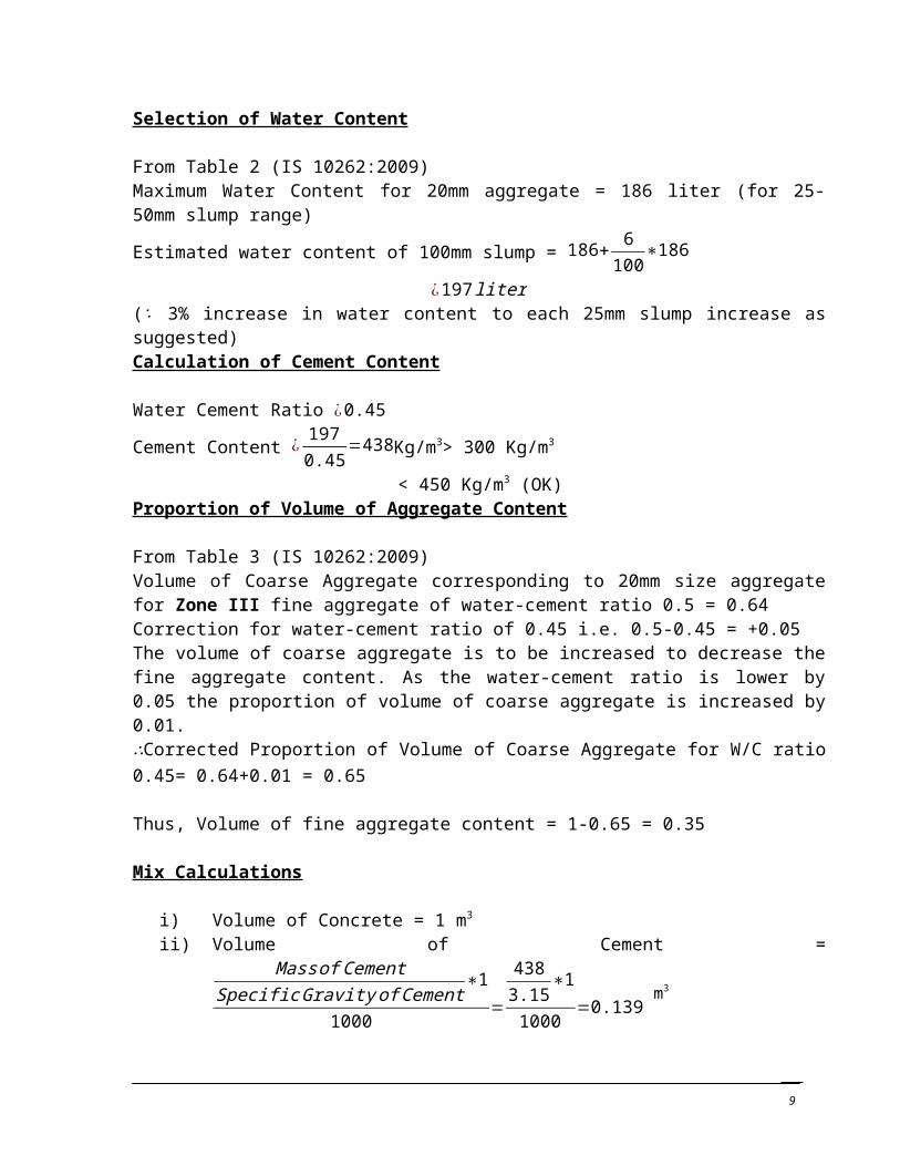
Selection of Water Content

From Table 2 (IS 10262:2009)Maximum Water Content for 20mm aggregate = 186 liter (for 25- 50mm slump range)

Estimated water content of 100mm slump = 186+ 6100

∗186

¿197 liter(∵ 3% increase in water content to each 25mm slump increase as suggested)Calculation of Cement Content

Water Cement Ratio ¿0.45

Cement Content ¿1970.45

=438Kg/m3> 300 Kg/m3

< 450 Kg/m3 (OK)Proportion of Volume of Aggregate Content

From Table 3 (IS 10262:2009)Volume of Coarse Aggregate corresponding to 20mm size aggregate for Zone III fine aggregate of water-cement ratio 0.5 = 0.64Correction for water-cement ratio of 0.45 i.e. 0.5-0.45 = +0.05The volume of coarse aggregate is to be increased to decrease the fine aggregate content. As the water-cement ratio is lower by 0.05 the proportion of volume of coarse aggregate is increased by 0.01.∴Corrected Proportion of Volume of Coarse Aggregate for W/C ratio 0.45= 0.64+0.01 = 0.65

Thus, Volume of fine aggregate content = 1-0.65 = 0.35

Mix Calculations

i) Volume of Concrete = 1 m3

ii) Volume of Cement = Mass of Cement

Specific Gravity of Cement∗1

1000=

4383.15

∗1

1000=0.139

m3

iii) Volume of Water =

Mass of waterSpecific Gravity of Water

∗1

1000=

1971000

=0.197 m3

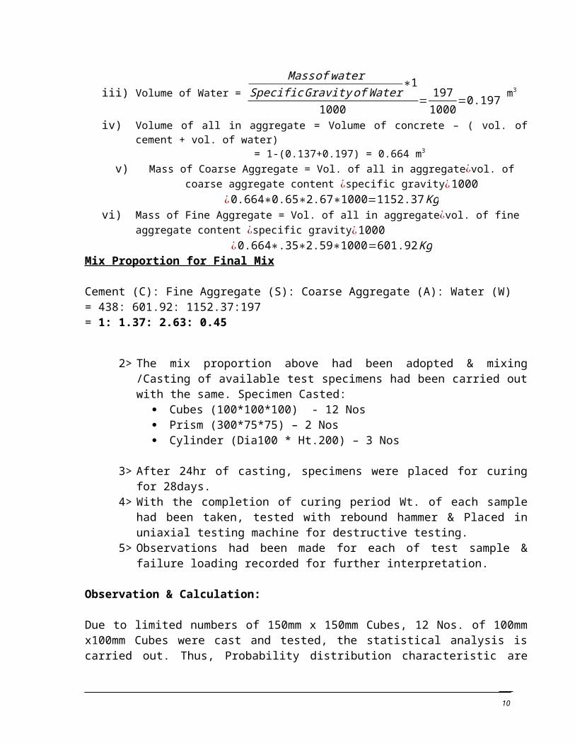
iv) Volume of all in aggregate = Volume of concrete – ( vol. of cement + vol. of water)= 1-(0.137+0.197) = 0.664 m3

v) Mass of Coarse Aggregate = Vol. of all in aggregate¿vol. of coarse aggregate content ¿specific gravity¿1000

¿0.664∗0.65∗2.67∗1000=1152.37 Kg

7

vi) Mass of Fine Aggregate = Vol. of all in aggregate¿vol. of fine aggregate content ¿specific gravity¿1000

¿0.664∗.35∗2.59∗1000=601.92 KgMix Proportion for Final Mix

Cement (C): Fine Aggregate (S): Coarse Aggregate (A): Water (W)= 438: 601.92: 1152.37:197= 1: 1.37: 2.63: 0.45

2> The mix proportion above had been adopted & mixing /Casting of available test specimens had been carried out with the same. Specimen Casted:

Cubes (100*100*100) - 12 Nos Prism (300*75*75) – 2 Nos Cylinder (Dia100 * Ht.200) – 3 Nos

3> After 24hr of casting, specimens were placed for curing for 28days.4> With the completion of curing period Wt. of each sample had been taken, tested with

rebound hammer & Placed in uniaxial testing machine for destructive testing.5> Observations had been made for each of test sample & failure loading recorded for

further interpretation.

Observation & Calculation:

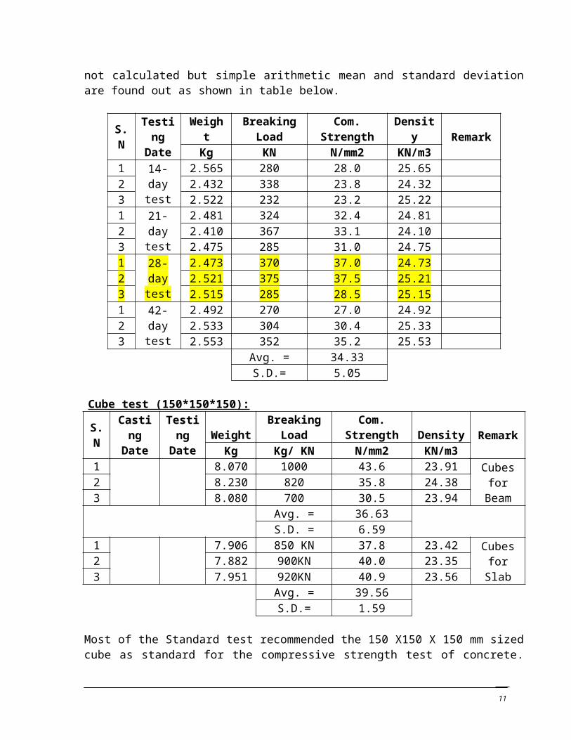
Due to limited numbers of 150mm x 150mm Cubes, 12 Nos. of 100mm x100mm Cubes were cast and tested, the statistical analysis is carried out. Thus, Probability distribution characteristic are not calculated but simple arithmetic mean and standard deviation are found out as shown in table below.

S.NTesting

DateWeight

Breaking Load

Com. Strength Density Remark

Kg KN N/mm2 KN/m31

14-day test

2.565 280 28.0 25.652 2.432 338 23.8 24.323 2.522 232 23.2 25.221

21-day test

2.481 324 32.4 24.812 2.410 367 33.1 24.103 2.475 285 31.0 24.751

28-day test

2.473 370 37.0 24.732 2.521 375 37.5 25.213 2.515 285 28.5 25.151

42-day test

2.492 270 27.0 24.922 2.533 304 30.4 25.333 2.553 352 35.2 25.53

Avg. = 34.33

8

S.D.= 5.05

Cube test (150*150*150):

S.NCasting

DateTesting

DateWeight

Breaking Load

Com. Strength Density Remark

Kg Kg/ KN N/mm2 KN/m31 8.070 1000 43.6 23.91

Cubes for Beam

2 8.230 820 35.8 24.383 8.080 700 30.5 23.94

Avg. = 36.63S.D. = 6.59

1 7.906 850 KN 37.8 23.42Cubes for

Slab2 7.882 900KN 40.0 23.353 7.951 920KN 40.9 23.56

Avg. = 39.56S.D.= 1.59

Most of the Standard test recommended the 150 X150 X 150 mm sized cube as standard for the compressive strength test of concrete. Since we cannot ignore other sized cubes, we have to develop correlation for different sizes cubes vs. compressive strength. Here we calculated multiplying factor for 100 X100 X 100 mm sized cube.

From the test data analysisFor 100mm Cube For 150mm CubeFavg= 34.33Mpa Favg= 39.6MpaS.D. = 5.05Mpa S.D. = 2.98 MpaFck= Favg-1.65 S.D. =25.99Mpa Fck= Favg-1.65 S.D. =34.683Mpa

Multiplying Shape Factor = 34.683/25.99 =1.33

Cylinder test (100-dia*200-ht.):

S.N

Casting Date

Testing Date

Weight Breaking LoadCom.

Strength Density Remark

Kg KN N/mm2 KN/m3

1

3.774

114

Comp.=10.89

24.03  Splitting TestPart11.578

Part21.97

3 Tensile= 3.632 3.822 187 23.8 24.33

Comp. Test3 3.800 195 24.83 24.19Avg. = 24.31

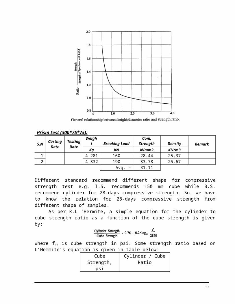
The strength of cylinder depends on the height (h) to the diameter (d) ratio of specimen as shown in graph below:

9

Prism test (300*75*75):

S.NCasting

DateTesting

DateWeight Breaking Load

Com. Strength Density Remark

Kg KN N/mm2 KN/m3

1 4.281 160 28.44 25.372 4.332 190 33.78 25.67

Avg. = 31.11

Different standard recommend different shape for compressive strength test e.g. I.S. recommends 150 mm cube while B.S. recommend cylinder for 28-days compressive strength. So, we have to know the relation for 28-days compressive strength from different shape of samples.

As per R.L ’Hermite, a simple equation for the cylinder to cube strength ratio as a function of the cube strength is given by:

Where fcu is cube strength in psi. Some strength ratio based on L’Hermite’s equation is given in table below:

Cube Strength, psi Cylinder / Cube Ratio3000 0.7654000 0.7905000 0.8096000 0.8257000 0.8388000 0.850

Table: Cylinder/Cube strength ratios Using L’Hermite’s equation

10

With the obtained data above, Simple analysis has been carried out for cube of size (100*100*100) & tabulated below.

Statistical Analysis SummaryMean 34.33Standard Deviation 5.05Variance 25.5Multiplying Factor 1.33Minimum 28.5Maximum 37.5Sum 103Count 3

Conclusions:

1. The Characteristic strength (fck) from uniaxial compression test (=25.99 MPa) is less than the targeted one (30Mpa) from mix design. The reason for less strength may be due to:

Non-uniform loading of uniaxial test machine (Small tilt found between end surface of test specimen & steel platen of test machine)

Presence of weak coarse aggregate(indicating the failure before the failure of aggregate - gel interface bond)

The cleanliness of coarse aggregate that may have affected bonding. Dimensional error in cube formwork due to unmanageable distortion.

2. The Standard Deviation was found to be 5.05 which is nearly equal to the adopted SD=5 indicating good quality control.

3. Compressive Strength of Cube (100*100*100) is obtained around 13% lower than the Cube (150*150*150). Therefore Cube (150*150*150) as Standard size, the size factor for Cube (100*100*100) is found 1.33.

11

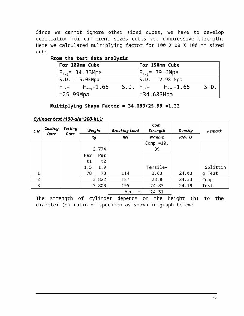
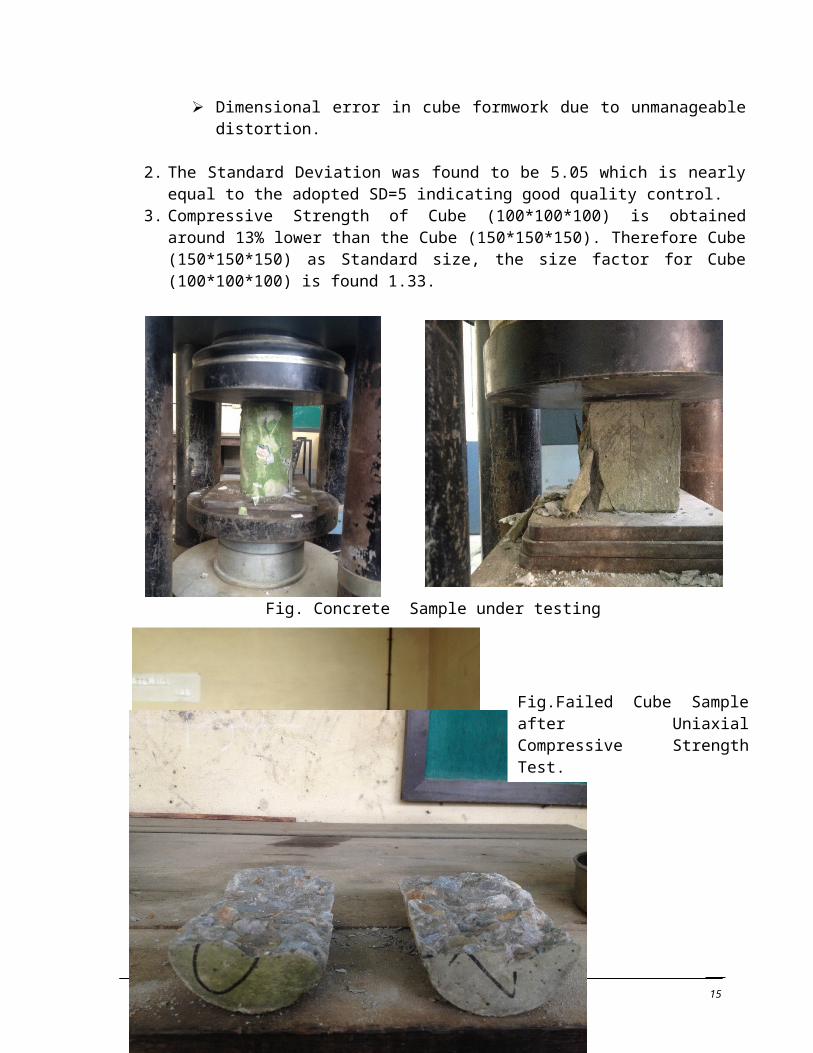
Fig. Concrete Sample under testing

Fig.Failed Cube Sample after Uniaxial Compressive Strength Test.

Fig.Failed Cube Sample after Uniaxial Compressive Strength Test.

Fig.Failed Cylinder Sample after Splitting Test. 12

Experiment no.2:

To study the mechanical response of RC Beam

Objective: To study the response of RC beam to the given loading condition.

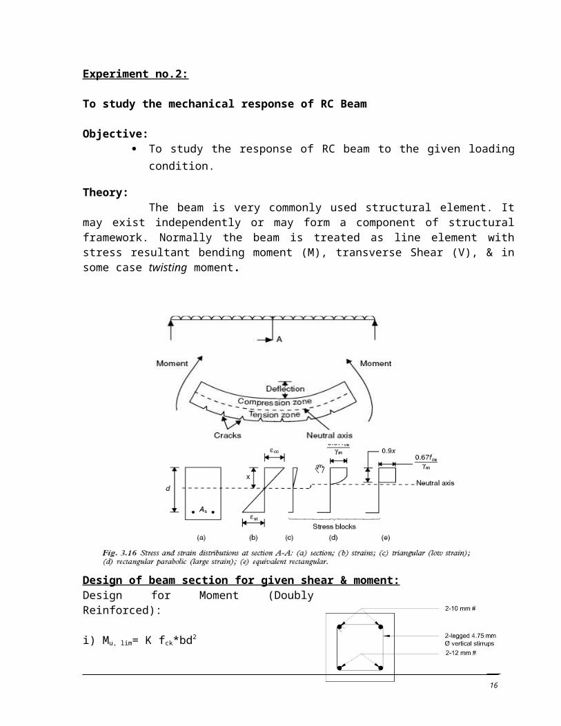
Theory:The beam is very commonly used structural element. It may exist independently or

may form a component of structural framework. Normally the beam is treated as line element with stress resultant bending moment (M), transverse Shear (V), & in some case twisting moment.

Design of beam section for given shear & moment:Design for Moment (Doubly Reinforced):

i) Mu, lim= K fck*bd2

Where, K= Constant depend upon fy.

ii) Pt, lim = 41.61 * fck∗Xu ,max

fy∗d

# Ast,lim= P t∗b∗d

100iii) Ast= Ast,lim+ ∆Ast

Where, ∆Ast = (Mu-Mu,lim)/.87fyd

13

iv) Asc =0.87 x fy x Δ Ast( fc−0.447 x fck )

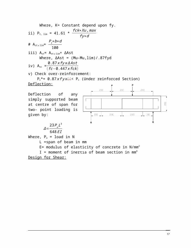
v) Check over-reinforcement: Pc*= 0.87 x f y x¿¿< Pc (Under reinforced Section) Deflection:

Deflection of any simply supported beam at centre of span for two- point loading is given by:

Δ=23 Pu L3

648 EIWhere, Pu = load in N

L =span of beam in mmE= modulus of elasticity of concrete in N/mm2

I = moment of inertia of beam section in mm4

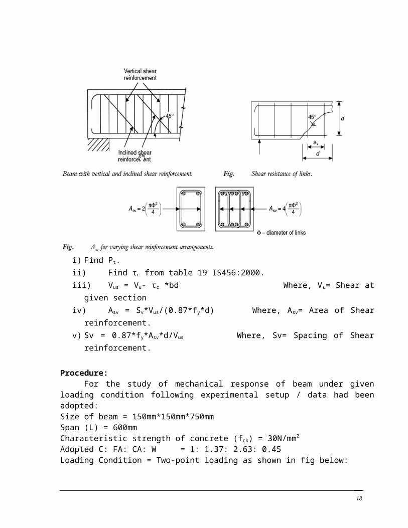
Design for Shear:

i) Find Pt.

ii) Find τc from table 19 IS456:2000.iii) Vus = Vu- τc *bd Where, Vu= Shear at given sectioniv) Asv = Sv*Vus/(0.87*fy*d) Where, Asv= Area of Shear reinforcement.v) Sv = 0.87*fy*Asv*d/Vus Where, Sv= Spacing of Shear reinforcement.

14

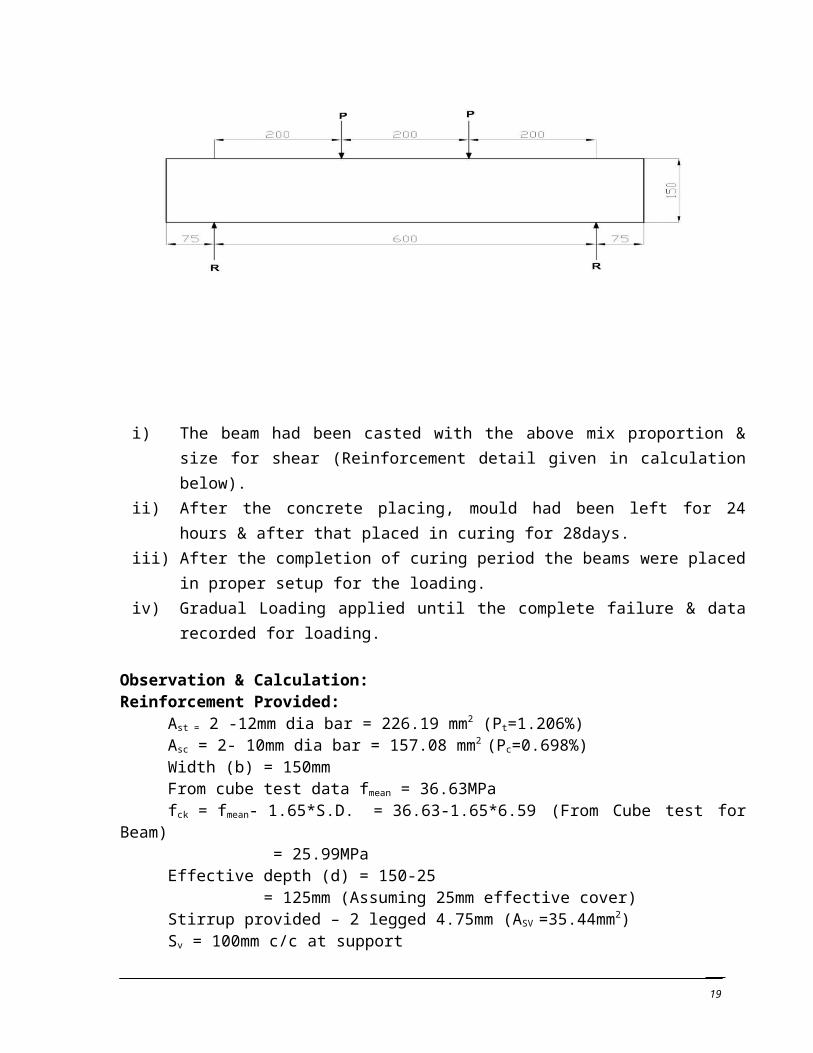
Procedure:For the study of mechanical response of beam under given loading condition following

experimental setup / data had been adopted:Size of beam = 150mm*150mm*750mmSpan (L) = 600mmCharacteristic strength of concrete (fck) = 30N/mm2

Adopted C: FA: CA: W = 1: 1.37: 2.63: 0.45Loading Condition = Two-point loading as shown in fig below:

i) The beam had been casted with the above mix proportion & size for shear (Reinforcement detail given in calculation below).

ii) After the concrete placing, mould had been left for 24 hours & after that placed in curing for 28days.

iii) After the completion of curing period the beams were placed in proper setup for the loading.

iv) Gradual Loading applied until the complete failure & data recorded for loading.

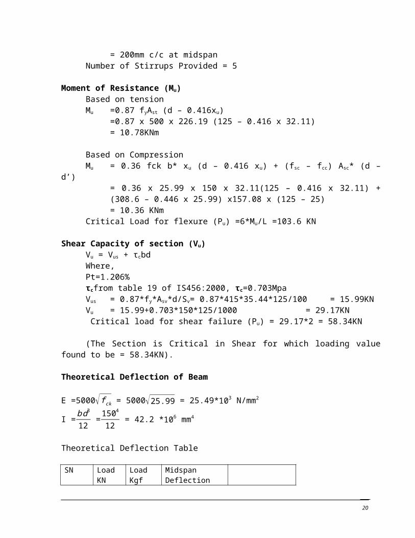
Observation & Calculation:Reinforcement Provided:

Ast = 2 -12mm dia bar = 226.19 mm2 (Pt=1.206%)Asc = 2- 10mm dia bar = 157.08 mm2 (Pc=0.698%)Width (b) = 150mmFrom cube test data fmean = 36.63MPafck = fmean- 1.65*S.D. = 36.63-1.65*6.59 (From Cube test for Beam)

= 25.99MPaEffective depth (d) = 150-25

= 125mm (Assuming 25mm effective cover)Stirrup provided – 2 legged 4.75mm (ASV =35.44mm2)Sv = 100mm c/c at support

15

= 200mm c/c at midspanNumber of Stirrups Provided = 5

Moment of Resistance (Mu)Based on tensionMu =0.87 fyAst (d – 0.416xu)

=0.87 x 500 x 226.19 (125 – 0.416 x 32.11)= 10.78KNm

Based on CompressionMu = 0.36 fck b* xu (d – 0.416 xu) + (fsc – fcc) Asc* (d – d’)

= 0.36 x 25.99 x 150 x 32.11(125 – 0.416 x 32.11) + (308.6 – 0.446 x 25.99) x157.08 x (125 – 25)= 10.36 KNm

Critical Load for flexure (Pu) =6*Mu/L =103.6 KN

Shear Capacity of section (Vu)Vu = Vus + τcbdWhere,Pt=1.206%τcfrom table 19 of IS456:2000, τc=0.703MpaVus = 0.87*fy*Asv*d/Sv= 0.87*415*35.44*125/100 = 15.99KNVu = 15.99+0.703*150*125/1000 = 29.17KN Critical load for shear failure (Pu) = 29.17*2 = 58.34KN

(The Section is Critical in Shear for which loading value found to be = 58.34KN).

Theoretical Deflection of Beam

E =5000√ f ck = 5000√25.99 = 25.49*103 N/mm2

I =b d3

12 =1504

12 = 42.2 *106 mm4

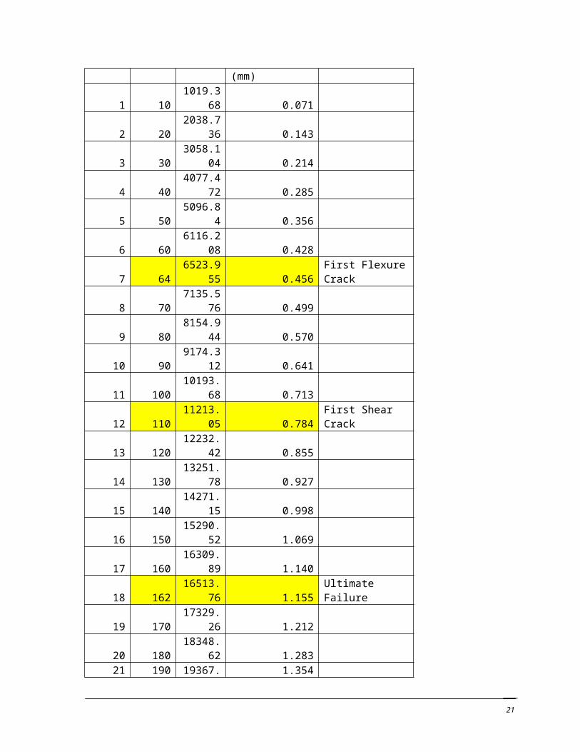
Theoretical Deflection Table

SN Load KN Load KgfMidspan Deflection (mm)

1 10 1019.368 0.0712 20 2038.736 0.1433 30 3058.104 0.2144 40 4077.472 0.2855 50 5096.84 0.3566 60 6116.208 0.4287 64 6523.955 0.456 First Flexure Crack8 70 7135.576 0.499

16

9 80 8154.944 0.57010 90 9174.312 0.64111 100 10193.68 0.71312 110 11213.05 0.784 First Shear Crack13 120 12232.42 0.85514 130 13251.78 0.92715 140 14271.15 0.99816 150 15290.52 1.06917 160 16309.89 1.14018 162 16513.76 1.155 Ultimate Failure19 170 17329.26 1.21220 180 18348.62 1.28321 190 19367.99 1.35422 200 20387.36 1.425

0 5000 10000 15000 20000 250000.000

0.200

0.400

0.600

0.800

1.000

1.200

1.400

1.600

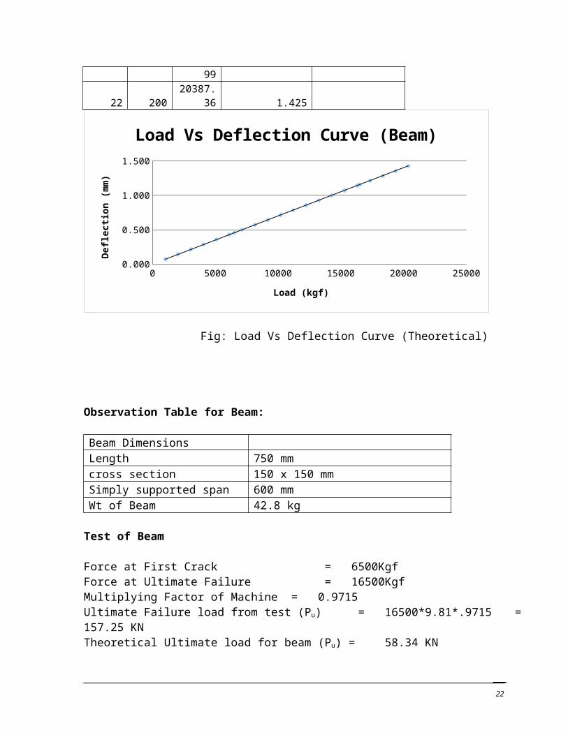
Load Vs Deflection Curve (Beam)

Load (kgf)

Defle

ction

(mm

)

Fig: Load Vs Deflection Curve (Theoretical)

Observation Table for Beam:

Beam DimensionsLength 750 mmcross section 150 x 150 mmSimply supported span 600 mmWt of Beam 42.8 kg

Test of Beam

17

Force at First Crack = 6500KgfForce at Ultimate Failure = 16500KgfMultiplying Factor of Machine = 0.9715Ultimate Failure load from test (Pu) = 16500*9.81*.9715 = 157.25 KNTheoretical Ultimate load for beam (Pu) = 58.34 KN

Conclusions:

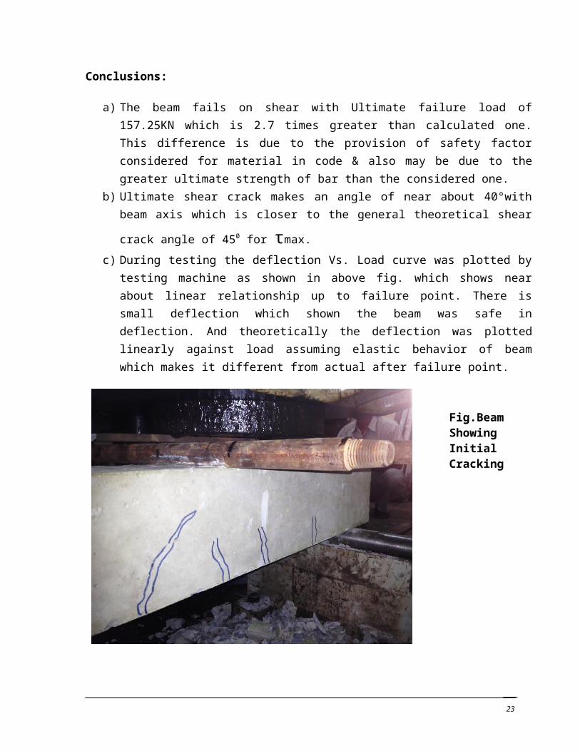
a) The beam fails on shear with Ultimate failure load of 157.25KN which is 2.7 times greater than calculated one. This difference is due to the provision of safety factor considered for material in code & also may be due to the greater ultimate strength of bar than the considered one.

b) Ultimate shear crack makes an angle of near about 40°with beam axis which is closer to

the general theoretical shear crack angle of 450 for τmax.

c) During testing the deflection Vs. Load curve was plotted by testing machine as shown in above fig. which shows near about linear relationship up to failure point. There is small deflection which shown the beam was safe in deflection. And theoretically the deflection was plotted linearly against load assuming elastic behavior of beam which makes it different from actual after failure point.

Fig.Beam Showing Initial Cracking

18

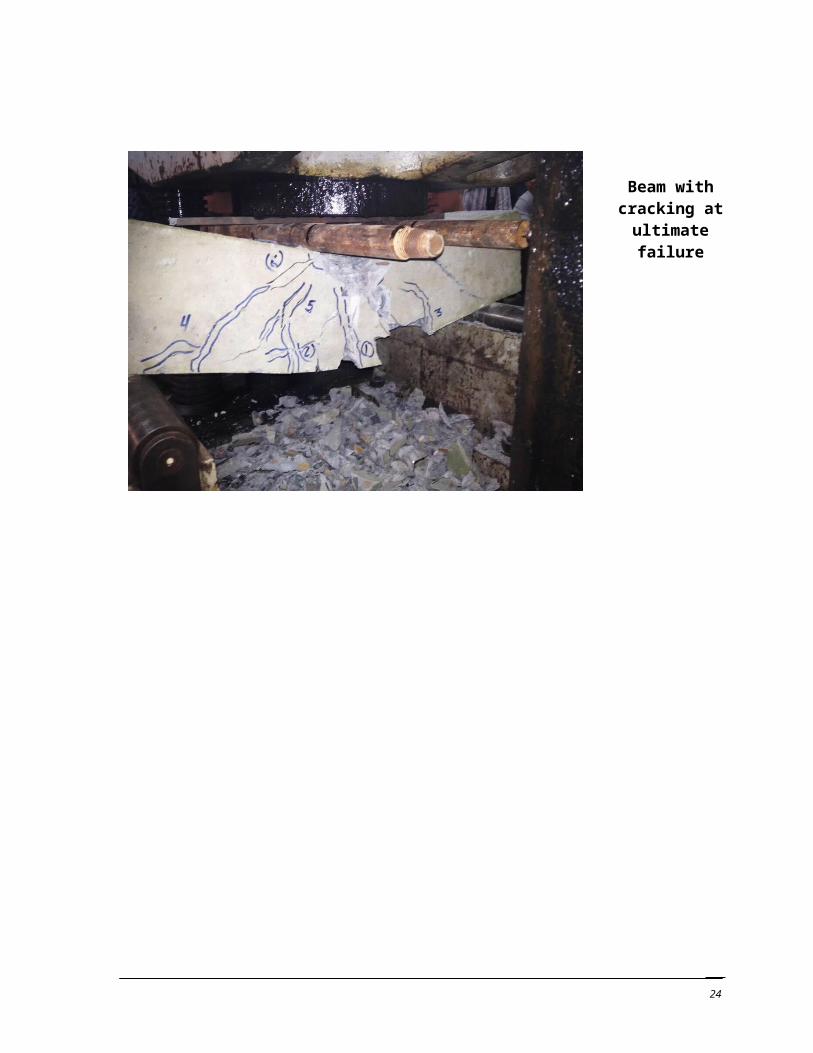
Beam with cracking at ultimate failure

19

Experiment no.3:

To study the mechanical response of RC Slab.

Objective:

To study the response of RC Slab under concentration load. To study the cracking pattern in slab under concentration load.

In short the objective is Yield Line Analysis and its Verification

Theory:

Slabs are generally considered as a plate element forming floor & roof structure carrying distributed or concentrated load primarily by flexure. Slabs may be simply supported or continuous over the support; flat slabs are supported at columns only.Slabs are designed using same theories of bending & shear as are used for beam. Following analysis are generally used for slab:

Elastic analysis. Semi empirical coefficient as given by code. Yield line theory.

Analysis of simply supported slab with concentrated load:1> Yieldlineanalysis.

20

- For rectangular yield line pattern Mu = Pu/8*L (where Mu= ultimate moment at mid span, Pu= ultimate loading)

- For circular yield line pattern Mu = Pu/2Π*L- For two side simply Supported Slab, Single yield line pattern, Mu =Pu*b/4L

2> From chart of Reynolds_Steedman’s Hand book:- Here mu = Pu*α*(ν+1)Where,

Pu= Ultimate loadingα= Coefficient From graphν= Poisson’s ratio.

Design for given moment:

M u=0.87∗f y∗A st∗d (1− f y∗A st

f ck∗b∗d )Procedure:

For the study of mechanical response of slab under given loading condition following experimental setup / data had been adopted:

Preliminary Design

Size of slab: 1000mm*1000mm*75mmSupport to support Span (L): 800mmCharacteristic strength of concrete (fck) =30 N/mm2

Mix Adopted C: FA: CA: W =1: 1.37: 2.63: 0.45Loading Condition = Concentrated loading as shown in fig below:With 20mm effective cover (d) = 75-20 =55mmfy=500 N/mm2

21

Provide 8mm dia. Bar @ 150mm C/CAst provided = 335.103 mm2 per m widthMu =7.203 KN-m per m widthFor Rectangular YL pattern, Mu=Pu/8*L

Pu=7.203*8*1= 57.626 KN

- Slab had been casted with the above mix proportion & size & reinforcements.- After the concrete placing, mould had been left for 24 hours & after that placed for curing

for 28days.- After the completion of curing period the slab was placed in proper setup for the loading.- Gradual Loading applied until the complete failure & data recorded for loading

Observation & Calculation:Compressive Strength Test (150mm Cubes)

S.N

Weight (Kg) Breaking load(KN)

Compressive Strength(MPa)

Density (Kg/m3)

Remark

1 7.906 850 37.8 23.4252 7.882 900 40 23.3543 7.951 920 40.9 23.559

Avg.= 39.6S.D.= 1.59

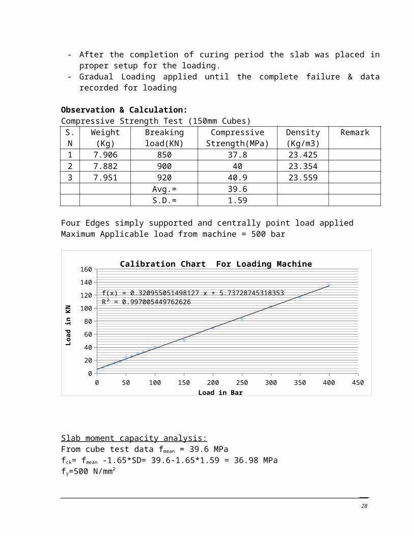
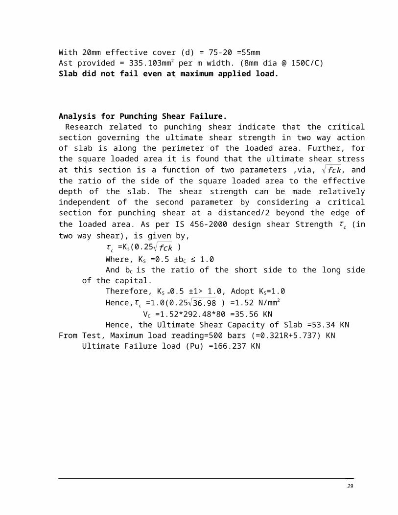
Four Edges simply supported and centrally point load appliedMaximum Applicable load from machine = 500 bar

0 50 100 150 200 250 300 350 400 4500

20

40

60

80

100

120

140

160

f(x) = 0.320955051498127 x + 5.73728745318353R² = 0.997005449762626

Calibration Chart For Loading Machine

Load in Bar

Load

in K

N

Slab moment capacity analysis:From cube test data fmean = 39.6 MPa

22

fck= fmean -1.65*SD= 39.6-1.65*1.59 = 36.98 MPafy=500 N/mm2

With 20mm effective cover (d) = 75-20 =55mmAst provided = 335.103mm2 per m width. (8mm dia @ 150C/C)Slab did not fail even at maximum applied load.

Analysis for Punching Shear Failure. Research related to punching shear indicate that the critical section governing the ultimate shear strength in two way action of slab is along the perimeter of the loaded area. Further, for the square loaded area it is found that the ultimate shear stress at this section is a function of two parameters ,via, √ fck , and the ratio of the side of the square loaded area to the effective depth of the slab. The shear strength can be made relatively independent of the second parameter by considering a critical section for punching shear at a distanced/2 beyond the edge of the loaded area. As per IS 456-2000 design shear Strength τ c (in two way shear), is given by,

τ c =Ks(0.25√ fck )Where, KS =0.5 ±bC ≤ 1.0And bC is the ratio of the short side to the long side of the capital.Therefore, KS =0.5 ±1> 1.0, Adopt KS=1.0Hence,τ c =1.0(0.25√36.98 ) =1.52 N/mm2

VC =1.52*292.48*80 =35.56 KNHence, the Ultimate Shear Capacity of Slab =53.34 KN

From Test, Maximum load reading=500 bars (=0.321R+5.737) KNUltimate Failure load (Pu) =166.237 KN

Fig.Slab Loading and Corner Support

Result:

23

Due to overstrength of slab and insufficient capacity of testing machine, the ultimate failure load for RCC Slab could not be determined. However, yield pattern in the slab along its center extending to free edges were observed.

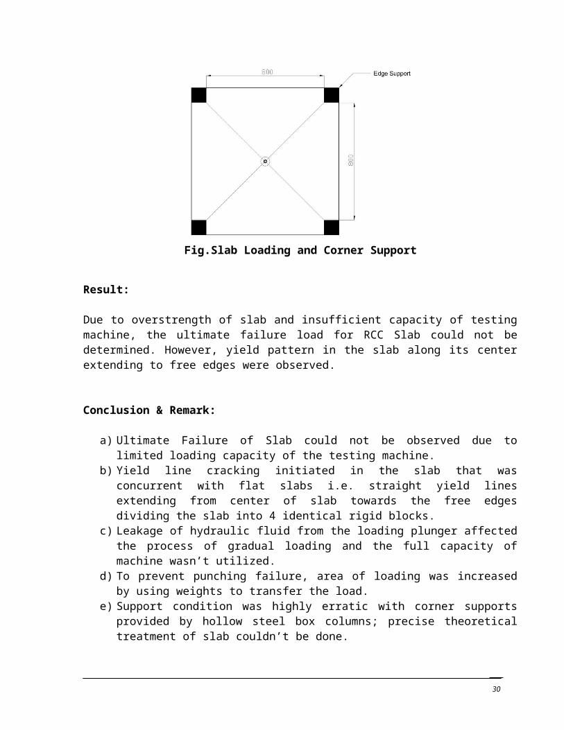
Conclusion & Remark:

a) Ultimate Failure of Slab could not be observed due to limited loading capacity of the testing machine.

b) Yield line cracking initiated in the slab that was concurrent with flat slabs i.e. straight yield lines extending from center of slab towards the free edges dividing the slab into 4 identical rigid blocks.

c) Leakage of hydraulic fluid from the loading plunger affected the process of gradual loading and the full capacity of machine wasn’t utilized.

d) To prevent punching failure, area of loading was increased by using weights to transfer the load.

e) Support condition was highly erratic with corner supports provided by hollow steel box columns; precise theoretical treatment of slab couldn’t be done.

Fig: Rebar Arrangement in Slab

24

Experiment no. 4:

Schmidt Hammer Test (Non Destructive Test)

Objective:

To obtain correlation curve for Schmidt Hammer and to obtain the compressive strength of existing structure using Schmidt (rebound) hammer.

Introduction:

Engineers worldwide use Original SCHMIDT Concrete Hammer to assess concrete quality and strength characteristics. It is a non-destructive test in which concrete can be tested in-situ condition. This instrument enables engineers to control concrete quality and to detect weak spot. As the test can be done in the site condition, strength of concrete can be evaluated in different time interval. The main advantage of this test is that it is easy to handle and it saves time.

Apparatus:

1. Schmidt Hammer2. Compression testing machine

Working Principle:

The Schmidt rebound hammer is principally a surface hardness tester. It works on the principle that the rebound of an elastic mass depends on the hardness of the surface against which the mass impinges. There is little apparent theoretical relationship between the strength of concrete and the rebound number of the hammer. However, within limits, empirical correlations have been established between strength properties and the rebound number. Further, Kolek has attempted to establish a correlation between the hammer rebound number and the hardness as measured by the Brinell method.

Procedure:

Selection of testing siteFirst of all the site for test has to be selected. The ceiling and inverted T-beam of heavy lab was selected.

Selection of the testing points:For slab, grid of 1m x 1m was marked where the tests have to be performed. Similarly, on beam points at a distance of 1m were selected. In order to get reliable results following factors are to be considered.

The plaster or coating must be removed. Cement slurry present in top layer must be removed.

Procedure for Schmidt Rebound Hammer Test:

25

The method of using the hammer is explained using figure With the hammer pushed hard against the concrete, the body is allowed to move away from the concrete until the latch connects the hammer mass to the plunger.The plunger is then held perpendicular to the concrete surface and the body pushed towards the concrete. This movement extends the spring holding the mass to the body. When the maximum extension of the spring is reached, the latch releases and the mass is pulled towards the surface by the spring.The method of using the hammer is explained using figure With the hammer pushed hard against the concrete, the body is allowed to move away from the concrete until the latch

connects the hammer mass to the plunger.The plunger is then held perpendicular to the concrete surface and the body pushed towards the concrete. This movement extends the spring holding the mass to the body. When the maximum extension of the spring is reached, the latch releases and the mass is pulled towards the plunger by the elastic energy released by spring. The mass hits the shoulder of the plunger rod and rebounds because the rod is pushed hard against the concrete. During rebound the slide indicator travels with the hammer mass and stops at the maximum distance the mass reaches after rebounding. A button on the side of the body is pushed to lock the plunger into the retracted position and the rebound number is read from a scale on the body.

Application of Schmidt Rebound Hammer Test:

The hammer can be used in the horizontal, vertically overhead or vertically downward positions as well as at any intermediate angle, provided the hammer is perpendicular to the surface under test. The position of the mass relative to the vertical, however, affects the rebound number due to the action of gravity on the mass in the hammer. Thus the rebound number of a floor would be

26

expected to be smaller than that of a soffit and inclined and vertical surfaces would yield intermediate results. Although a high rebound number represents concrete with a higher compressive strength than concrete with a low rebound number. A typical correlation procedure is, as follows:

1. Prepare a number of cylinders or cube specimens 2. Take hammer rebound readings of each cube, take at least 5 readings, and ensure that the

cubes are in surface dry condition.3. Avg. the readings and call this the rebound number for the cube.4. Test the cylinders to failure in compression and plot the rebound numbers against the

compressive strength.5. Fit a curve or a line by the method of least squares

Limitations of Schmidt Rebound Hammer Test:

1. Smoothness of the test surfaceHammer has to be used against a smooth surface, preferably a formed one. Open textured concrete cannot therefore be tested.

2. Size, shape and rigidity of the specimen If the concrete does not form part of a large mass any movement caused by the impact of the hammer will result in a reduction in the rebound number. In such cases the member has to be rigidly held or backed up by a heavy mass.

3. Age of test specimenFor equal strengths, higher rebound numbers are obtained with a 7 day old concrete than with a 28 day old. Therefore, when old concrete is to be tested in a structure a direct correlation is necessary between the rebound numbers and compressive strengths of cores taken from the structure.

4. Surface and internal moisture conditions of concreteThe rebound numbers are lower for well-cured air dried specimens than for the same specimens tested after being soaked in water and tested in the saturated surface dried conditions. Therefore, whenever the actual moisture condition of the field concrete or specimen is unknown, the surface should be pre-saturated for several hours before testing.

5.Type of coarse aggregateDifferent researchers have obtained varying results in relationship between aggregate type, rebound number and strength correlation. Variations in compressive strength in order of 7MPa (difference of 7 in rebound number) were observed in cylinders with limestone coarse aggregate (lower) and crushed stone aggregate (higher) [Kliegar et. al.]. For similar aggregate from different sources, variation in strength of 1.7 to 3.9 MPa was observed for same rebound number (Grieb et. al). Variation for lightweight aggregate was studied by Greene.However, in all above cases, compressive strength of aggregate was proportional to rebound number.

6. Type of Cement

27

According to Kolek the type of concrete significantly affects the rebound number readings. High concrete can have actual strengths 100% higher than those obtained using a correlationcurve based on concrete made with ordinary portland cement. Also, supersulfated cementconcrete canhave 50% lower strength than obtained from the ordinary portland cement concrete correlation curves.

7. Type of MoldMitchell and Hoagland have carried out studies to determine the effect of the type of concrete moldon the rebound number. When cylinders cast in steel, tin can, and paper carton molds were tested, therewas no significant difference in the rebound readings between those cased in steel molds and tin canmolds, but the paper carton-molded specimens gave higher rebound numbers. This is probably due tothe fact that paper molds withdraw moisture from the fresh concrete, thus lowering the water-cementratio at the surface and resulting in a higher strength. As the hammer is a surface hardness tester, it ispossible in such cases for the hammer to indicate an unrealistically high strength. It is therefore suggestedthat if paper carton molds are being used in the field, the hammer should be correlated against thestrength results obtained from test cylinders cast in similar molds.

Observation and Calculation:

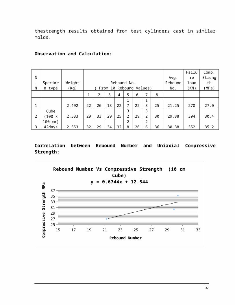
Correlation between Rebound Number and Uniaxial Compressive Strength:

28

S.N

Specimen type

Weight (Kg)

Rebound No.( From 10 Rebound Values)

Avg. Rebound

No.

Failure load (KN)

Comp. Strength (MPa)

1 2 3 4 5 6 7 8

1 Cube(100 x 100

mm)42days

2.492 22 26 18 22 17 22 18 25 21.25 270 27.0

2 2.533 29 33 29 25 32 29 32 30 29.88 304 30.4

3 2.553 32 29 34 32 28 26 26 36 30.38 352 35.2

15 17 19 21 23 25 27 29 31 3325

27

29

31

33

35

37

Rebound Number Vs Compressive Strength (10 cm Cube)y = 0.6744x + 12.544

Rebound Number

Com

pres

sive

Stre

ngth

MPa

29

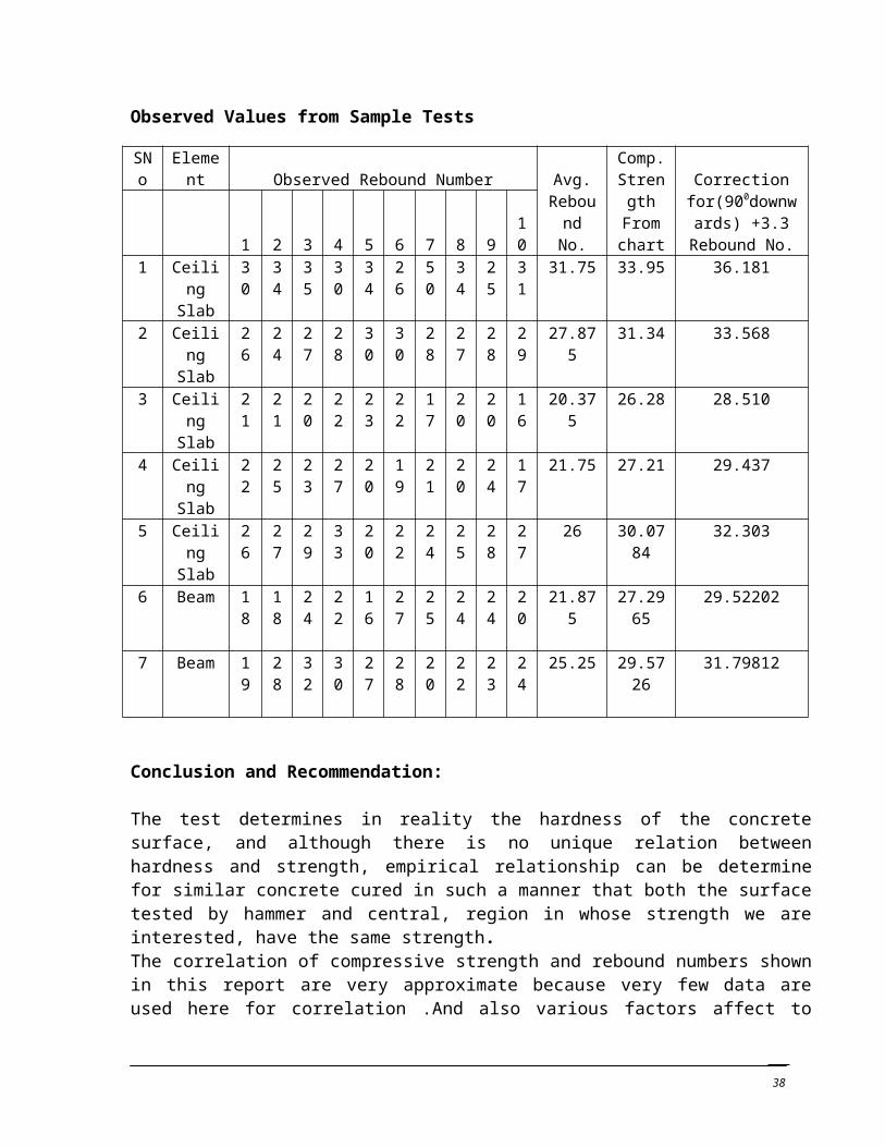
Observed Values from Sample Tests

SNo

Element Observed Rebound Number Avg. 

Rebound No.

Comp. Strength From chart

Correction for(9

00downwards) +3.3 Rebound No.1 2 3 4 5 6 7 8 9

10

1 Ceiling Slab

30 34

35

30

34

26

50

34

25

31

31.75 33.95 36.181

2 Ceiling Slab

26 24

27

28

30

30

28

27

28

29

27.875 31.34 33.568

3 Ceiling Slab

21 21

20

22

23

22

17

20

20

16

20.375 26.28 28.510

4 Ceiling Slab

22 25

23

27

20

19

21

20

24

17

21.75 27.21 29.437

5 Ceiling Slab

26 27

29

33

20

22

24

25

28

27

26 30.0784

32.303

6 Beam 18 18

24

22

16

27

25

24

24

20

21.875 27.2965

29.52202

7 Beam 19 28

32

30

27

28

20

22

23

24

25.25 29.5726

31.79812

Conclusion and Recommendation:

The test determines in reality the hardness of the concrete surface, and although there is no unique relation between hardness and strength, empirical relationship can be determine for similar concrete cured in such a manner that both the surface tested by hammer and central, region in whose strength we are interested, have the same strength.The correlation of compressive strength and rebound numbers shown in this report are very approximate because very few data are used here for correlation .And also various factors affect to find the compressive strength accurately such as surface condition of tested specimen, presence of large aggregate at test point, other manual unseen errors, etc. However the objective of Schmidt Hammer test and detailed procedure are well known from this experimentThis test is a comparative nature only. In particular, the hardness of concrete depends on elastic properties of the aggregate used and may also affected by large differences in proportions and by carbonation.Though the actual strength of slab tested is not known to compare with the experiment result, the strength of the Slab, Beam, and column a 95% confidence level is computed. The result of the Beam is lesser obtained because of various error during observation.

30

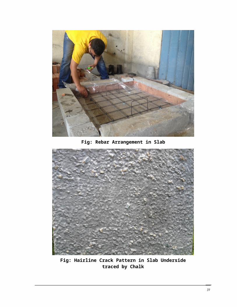
Fig. Schmidt Hammer

Comment:Due to faulty instrument, the correlation chart generated above is of no importance in determining the strength of structural elements tested for practice by rebound hammer. The practice tests were carried out in the existing college building and as such, the plaster covers were not scraped to reveal the concrete surface. Thus the collected data for ceiling and beams are only representative for vertically downward orientation and horizontal direction of Schmidt Hammer. Correlation with above chart for horizontal loading is done

31

Experiment no. 5

Ultrasonic Pulse Velocity Test (Non Destructive Test)

Objective:

To determine the strength of concrete by measuring the Ultrasonic Pulse velocity through the concrete specimen and hence to determine the modulus of elasticity of the concrete.

Introduction:

It is the non-destructive test, which is used to determine the longitudinal ultrasonic pulse velocity in concrete structure through which the wave is propagated. There is no unique relationship between these velocity and strength of concrete but under specified conditions these two quantities are related. The common factor is a density of concrete, a change in the density results in a change in the pulse velocity. If the velocity of a pulse of longitudinal waves through a medium can be determined, and if the density and Poisson’s ratio of the medium is known, then the dynamic modulus of elasticity can be computed.

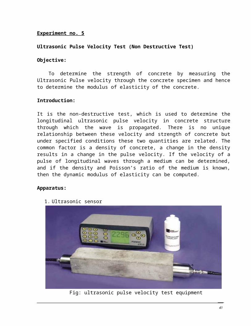
Apparatus:

1. Ultrasonic sensor

Fig: ultrasonic pulse velocity test equipment

Working Principle:

A pulse of longitudinal vibrations is produced by an electro-acoustical transducer, which is held in contact with one surface of the concrete under test. When the pulse generated is transmitted into the concrete from the transducer using a liquid coupling material such as grease or cellulose paste, it undergoes multiple reflections at the boundaries of the different material phases within the concrete. A complex system of stress waves develops, which include both longitudinal and shear waves, and propagates through the concrete. The first waves to reach the receiving

32

transducer are the longitudinal waves, which are converted into an electrical signal by a second transducer. Electronic timing circuits enable the transit time T of the pulse to be measured.Longitudinal pulse velocity (in km/s or m/s) is given by:

V=L/TWhere,V is the longitudinal pulse velocity,

L is the path length,T is the time taken by the pulse to traverse that length.

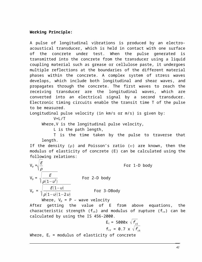
If the density () and Poisson’s ratio () are known, then the modulus of elasticity of concrete (E) can be calculated using the following relations:

Vp =√ Eρ

For 1-D body

Vp = √ Eρ(1−υ2)

For 2-D body

Vp = √ E (1−υ )ρ (1−υ)(1−2 υ)

For 3-DBody

Where, Vp = P – wave velocityAfter getting the value of E from above equations, the characteristic strength (fck) and modulus of rupture (fcr) can be calculated by using the IS 456-2000. Ec = 5000x √ f ck

fcr = 0.7 x √ f ck

Where, Ec = modulus of elasticity of concrete fck = characteristic strength of concrete fcr = modulus of rupture of concrete

Equipment for pulse velocity

The equipment consists essentially of an electrical pulse generator, a pair of transducers, an amplifier and an electronic timing device for measuring the time interval between the initiation of a pulse generated at the transmitting transducer and its arrival at the receiving transducer. Two forms of electronic timing apparatus and display are available, one of which uses a cathode ray tube on which the received pulse is displayed in relation to a suitable time scale, the other uses an interval timer with a direct reading digital display

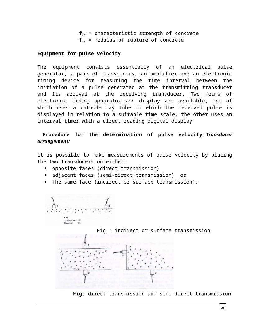
Procedure for the determination of pulse velocity Transducer arrangement:

It is possible to make measurements of pulse velocity by placing the two transducers on either: opposite faces (direct transmission) adjacent faces (semi-direct transmission) or The same face (indirect or surface transmission).

33

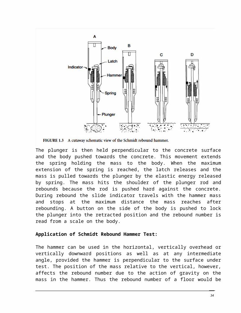
Fig : indirect or surface transmission

Fig: direct transmission and semi-direct transmission

Note: It is better to use the direct transmission arrangement since the transfer of energy between transducers is at its maximum and the accuracy of velocity determination is therefore governed principally by the accuracy of the path length measurement. The couplant used should be spread as thinly as possible to avoid any end effects resulting from the different velocities in couplant and concrete.

Coupling the transducer onto the concrete:

To ensure that the ultrasonic pulses generated at the transmitting transducers pass into the concrete and are then detected by the receiving transducer, it is essential that there is adequate acoustical coupling between the concrete and the face of each transducer. For many concrete surfaces, the finish is sufficiently smooth to ensure good acoustical contact by the use of a coupling medium and by pressing the transducer against the concrete surface. Typical couplants are petroleum jelly, grease, soft soap and kaolin/glycerol paste. It is important that only a very thin layer of coupling medium separates the surface of the concrete from its contacting transducer. For this reason, repeated readings of the transit time should be made until a minimum value is obtained so as to allow the layer of the couplant to become thinly spread.

Factors influencing pulse velocity measurements

Moisture content:The moisture content has two effects on the pulse velocity, one chemical the other physical. Between a properly cured standard cube and a structural element made from the same concrete, there may be a significant pulse velocity difference. Much of the difference is accounted for by the effect of different curing conditions on the hydration of the cement while some of the difference is due to the presence of free water in the voids.

Temperature of the concrete:

34

Variations of the concrete temperature between 10 0C and 30 0C have been found to cause no significant change without the occurrence of corresponding changes in the strength or elastic properties.

Path length:The path length over which the pulse velocity is measured should be long enough not to be significantly influenced by the heterogeneous nature of the concrete. The pulse velocity is not generally influenced by changes in path length, although the electronic timing apparatus may indicate a tendency for velocity to reduce slightly with increasing path length. Effect of reinforcing bars:The pulse velocity measured in reinforced concrete in the vicinity of reinforcing bars is usually higher than in plain concrete of the same composition. This is because the pulse velocity in steel may be up to twice the velocity in plain concrete and, under certain conditions, the first pulse to arrive at the receiving transducer travels partly in concrete and partly in steel.

Concrete uniformity:Heterogeneities in the concrete within or between members cause variations in pulse velocity, which in turn are related to variations in quality. Measurements of pulse velocity provide a means of studying the homogeneity.

Reliability and Discrepancy:

Ultrasonic pulse velocity technique is more reliable than rebound hammer teat because it gives information about the state of concrete throughout width or depth of structure member. The technique used as a means of quality control of products, which are supposed to be made of similar concrete. Both lack of compaction and change in w/c ratio would be easily detected. As per Whitehurst, for concrete of density of approximate 24 KN/m3, the relation between longitudinal velocities in Km/s and quality of concrete are as follows

V (Km/s) Quality of Concrete>4.5 Excellent

3.5-4.5 Good3.0-3.5 Doubtful2.0-3.0 Poor

<2.0 Very poorProcedure:

Cubes of 100 mm were prepared as usual procedure. Time taken by the pulse in microsecond to travel from one face of the cube to other face

was found out for each cube. After then compressive strength test was conducted (destructive). The correlation between pulse velocity and cube compressive strength was prepared.

Finally Young’s modulus of elasticity of concrete was computed.

Observation and Calculation

35

Since, due to the improper functioning of ultrasonic sensor we were not able to make observation in our specimen.

Discussion:

Pulse velocity isless for low strength concrete then high strength concrete. It is because of the high strength concrete is more compact than low strength concrete.To develop exact correlation, more specimens (at least 15 nos.) are required. The computed characteristic strength of the concrete is less than the observed value.The ultrasonic pulse velocity test, although approximate, can be used as a means of computing compressive strength quickly and easily in field using the correlation charts developed.In order to access the field strength near to the exact value, the calibration chart used shall of being prepared very carefully, and in a condition approximately near to the field condition.

36

Experiment No: 6

Cover meter (Profometer) Test (Non Destructive Test)

Objective:

To study the working principle of cover meter and its applications

Introduction:

Cover meter is a sophisticated device for the non destructive location of rebars and for the measurement of concrete cover and bar diameters, using the eddy current principle with pulse induction as the measuring method as well as detecting the rebar diameter accurately to the millimeter by only one measuring procedure.Cover meter is an instrument to locate rebar and measure the exact concrete cover. Rebar detectors are sophisticated devices that can locate metallic objects below the surface. Due to the cost-effective design, the pulse-induction method is one of the most commonly used solutions.Concrete cover is the distance from the surface of the concrete to the surface of the reinforcing bars embedded in the concrete. Ensuring sufficient concrete cover is critical for the durability of some concrete structures subject to poor environment during their service life, such as seawater desalination plants, jetties, bridges and reservoirs etc. Concrete cover can be measured using commercially available cover meter such as Profometer. The assessment of concrete cover for such important concrete structures should be only based on accurate measurement results by professionals.

Application:

Locate rebars  with the cover meter to avoid them when drilling holes Acceptance inspection of cover after formwork is removed Measuring concrete cover depth with the cover meter Quality assurance in mass production of prefabricated concrete elements

Method:

37

The pulse-induction method is based on electromagnetic pulse induction technology to detect rebars. Coils in the probe are periodically charged by current pulses and thus generate a magnetic field. On the surface of any electrically conductive material which is in the magnetic field eddy currents are produced. They induce a magnetic field in opposite directions. The resulting change in voltage can be utilized for the measurement. Rebars that are closer to the probe or of larger size produce a stronger magnetic field.Modern rebar detectors use different coil arrangements to generate several magnetic fields. Advanced signal processing supports not only the localization of rebars but also the determination of the cover and the estimation of the bar diameter. This method is unaffected by all non conductive materials such as concrete, wood, plastics, bricks etc. However any kind of conductive materials within the magnetic field will have an influence on the measurement. Advantages of the pulse induction method:

high accuracy not influenced by moisture and non-homogeneities of the concrete unaffected by environmental influences Low costs.

Disadvantage of the pulse induction method: Limited detection range Minimum bar spacing depends on cover depths

Cover Meter Accuracy and Factors Affecting Cover Measurement :

Each measurement comes with certain variation and every measuring equipment has its own accuracy. Cover meter is one of such measuring equipments. Many factors can affect cover measurement. These include neighboring bars parallel to the bar being measured, setting of bar diameter during cover measurement, scan location relative to secondary bars under the bar being measured, different measurement probes (deep or shallow) or different probe settings (low or high range for cover meters using universal probe) etc. Other factors such as magnetic effects from the aggregate or matrix of the concrete, variations in the properties of the steel, cross-sectional shape of bars and rib height, roughness of the surface can also influence cover measurement. However, these factors are insignificant compared to former factors. Only limited research on cover meter accuracy is available.

38

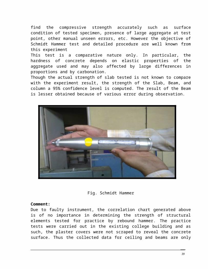
Fig: Cover meter

Comments:Profometer available in the laboratory was damaged and couldn’t be used for locating reinforcement in slabs to map out rebar arrangement during core cutting. Only the theoretical aspect of pulse-induction method was studied in textbook. Practical application wasn’t carried out.

39

Experiment No: 7

To measure the compressive strength of concrete by Core Testing

Objective:

To study the process of core sampling and testing

Theory:

Core testing is a destructive test, and is beneficial when the results obtained from the cube or cylindrical specimens are below the specific value. Thus, two possibilities appear, either the concrete is very weak, or the specimens are not correctly prepared and so not representative to the concrete in the structure. So core cylinders are obtained from the structure with a height to diameter ratio of 2:1. The obtained core specimen then shall be cured, capped and then tested compression in moist condition.

The empty place of the core shall then be filled with materials that give the same strength, and in cases of steel existence the steel is welded with other thicker steel in the hole. The core specimen is obtained by means of using a core drilling machine.

Principal:

This is the method based on destructive test in which the core cutting is done in the existing structure to test the strength of the concrete. The core cutting machine will cut the core in specified place. Once the concrete has been cut, it is tested on the compression testing machine.

Apparatus Required:i) Core drillii) Specimen for testiii) Water pump

Procedure:

i) The specimen is checked for the reinforcement embedment by pachometer.ii) The specimen is marked to the point where core cutting is done.iii) Core drilling machine is place over the mark for the core specimen.iv) Once the machine get started to the specified point, the machine get start to cut the

core. v) Water is continuously applied to the machine so that the heat generation is reduced.vi) After some time, the machine completely cut the specimen into a cylindrical shape,

known as core specimen.vii) Once we get the specimen, it is tested in the compression machine.

40

Observation and Result:

S.N. Weight (Kg)

Breaking Load (KN)

Strength (Mpa)

Correction Factor

Actual Strength(Mpa)

1 2.119 180 22.92 1.726 39.56

The strength of cylinder depends on the height (h) to the diameter (d) ratio of specimen as shown in graph below:

Conclusion and Discussion:From the above experiment we found that, the compressive strength of the slab that we have casted is 39.56 MPa in average with standard deviation of 1.59 MPa.The design strength of the slab is M30, and we are testing for the same slab. The variation that we observed from our real strength of the slab is due to various reasons such as: a vibration that the core cutting machine produce itself forms a microcracks, non- continuity for the cutting sample while cutting, surface is not perfectly smooth and horizontal to gain the strength etc. One of the bars was cut in the core as we couldn’t identify the rebar location exactly in absence of profometer. This resulted in anomalous value of compressive strength.

Due to lack of time, capping of core wasn’t done and hence, due to irregularity of top surface, breaking strength obtained was quite low than expected.These core cutting is excessively used in bridges to assurence for the quality of concrete, for reparing works.The use of this method gives reliable results for compressive strength as the specimen is taken directly from the structure, so it will be representative for the whole structure.

41

Since these tests are destructive tests, the hole that the core cutting machine made should be sealed with the same or more quality with fast hardening cement in the real field. If the rod gets cut during core cutting the rods should be welded and filled with concrete.

Thus we have successfully complete our core cutting experiment.

The images of core cutting operation and sample core is presented below.

Fig: Core Cutting Operation in progress

Fig: Slab after core cutting

Fig: Handling of Core for testing

42

BibliographyC.E Reynolds, R. S. (n.d.). Reinforced Concrete Designer's

Handbook. EF & N SPON .Concrete. (2000). Concrete: Microstructure Properties and

Materials. Tata MCGraw Hill.Inc., D.-C. (2009). Duro-Crete Concrete Mix Manual.R. Park, W. G. (2000). Reinforced Concrete Slabs.S UnniKrishna Pillai, D. M. (n.d.). Reinforced Concrete Design.

Tata McGraw Hill.V M Malhotra, N. J. (n.d.). Nondestructive Testing of Concrete.

43